


1. Introduction
This note concerns the cross-country size distribution of government debt, commonly measured as the debt-to-GDP ratio (in %). Traditionally, the size distribution of government debt has been parameterized as lognormal. From a theoretical perspective, Barro (Reference Barro1979), constructing a model of public debt for a large national government, states:
“The theory predicts that the level of debt or the debt-to-income ratio would be irrelevant for current debt issue. […] This result supports the surprising proposition of the theory that the debt-to-income ratio does not have a ‘target’ value but rather moves ‘randomly’.”
From an empirical standpoint, Barro (Reference Barro1979) documents size-independent proportional growth of the debt-to-GDP ratio by regressing the growth rate of public debt against the level of debt and finding the estimated coefficient to be insignificantly different from zero. Much of the ensuing literature has also treated the size of the debt-to-GDP ratio as a unit root process and hence nonstationary (Bohn, Reference Bohn1998).
The above characterizations and empirical evidences for the size and growth rate of the debt-to-GDP ratio are largely consistent with a process adhering to random multiplicative growth, more commonly referred to as Gibrat’s law of proportionate random growth (Sutton, Reference Sutton1997; Gabaix, Reference Gabaix2009). It is well known that random multiplicative growth, in its purest form, gives rise to a lognormal distribution, which conceivably justifies the prevailing practice of adopting the lognormal distribution for modeling the size distribution of government debt. However, Gibrat’s law can similarly generate a power law (Pareto) distribution (Gabaix, Reference Gabaix1999; Reed, Reference Reed2001), and the double Pareto-lognormal (dPLN) in particular, which is the product of independent double Pareto and lognormal distributions (Reed, Reference Reed2003; Reed and Jorgensen, Reference Reed and Jorgensen2004).
For power law, and dPLN, to arise as the stationary distribution, a random multiplicative growth process needs some friction (Gabaix, Reference Gabaix2009). Among several generative mechanisms of power law and dPLN (Reed, Reference Reed2001, Reference Reed2003; Toda, Reference Toda2014, Reference Toda2017; Beare et al. Reference Beare, Seo and Toda2022; Beare and Toda, Reference Beare and Toda2022), a random multiplicative growth process with random resets (Reed, Reference Reed2001; Beare and Toda, Reference Beare and Toda2022) stands out. The theory essentially posits that economic units experience random multiplicative shocks to their size through time until stopped (perishing) at random and being replaced by a new unit. For our empirical context, this would imply government debt evolves over time according to random multiplicative growth and is occasionally reset, perhaps due to sovereign default. This appears entirely reasonable since, as Barro (Reference Barro1979) pointed out:
“[T]here may be a wide range within which the debt-income ratio can vary essentially freely […] but there may be some eventual limits that come into play. A limit on the high side would arise when the debt-income ratio rises sufficiently to affect the probability of the government’s default.”
The plausibility of the random resetting mechanism in capturing the key features of the empirical context positions it as a valid alternative to the conventionally adopted pure random multiplicative growth process. This, in turn, raises the need for a thorough empirical examination of the size distribution of government debt across the entire cross-section and its evolution over time. If the debt-to-GDP ratio follows a dPLN distribution, it would provide indirect evidence suggesting that debt-to-GDP obeys the generative mechanism of dPLN—a random resetting mechanism. Conversely, if the debt-to-GDP ratio is lognormal, it would offer indirect evidence in favor of a pure random multiplicative growth process. The present article seeks to address this issue.
Our analysis demonstrates that the lognormal distribution tends to provide a reasonable fit to the cross-sectional distribution of debt-to-GDP ratios for the period between 1980 and 2000. However, significant departures from lognormality are observed in the post-2000 debt data. In contrast, the dPLN fits the data remarkably well across all periods, whether in terms of model fit criteria or goodness-of-fit tests. While the dPLN fits the data at least as well as the lognormal during 1980–2000, it straightly outperforms the lognormal and other candidate distributions in the post-2000 period.
Why does this finding matter? The finding has several noteworthy economic, econometric, and social implications, as elaborated next.
First, it indicates that the debt-to-GDP ratio follows a ubiquitous empirical regularity, the power law,Footnote 1 in both its upper and lower tails. For the upper tail, this means that the fraction of units above size $x$
is roughly proportional to
$x$
is roughly proportional to $x^{-\alpha }$
, where
$x^{-\alpha }$
, where $\alpha \gt 0$
is the upper-tail power law exponent. Similarly, for the lower tail, it implies that the fraction of units below size
$\alpha \gt 0$
is the upper-tail power law exponent. Similarly, for the lower tail, it implies that the fraction of units below size $x$
is approximately proportional to
$x$
is approximately proportional to $x^{\beta }$
, where
$x^{\beta }$
, where $\beta \gt 0$
is the lower-tail power law exponent. Several recent studies, including those by Toda (Reference Toda2012) on income and Toda (Reference Toda2017) on consumption, have shown the dPLN’s superiority in fitting size distributions previously described by lognormal or Pareto distributions. Methodologically, our work contributes to this literature by documenting the dPLN’s robust fit to, and the power law behavior of, the size distribution of government debt.
$\beta \gt 0$
is the lower-tail power law exponent. Several recent studies, including those by Toda (Reference Toda2012) on income and Toda (Reference Toda2017) on consumption, have shown the dPLN’s superiority in fitting size distributions previously described by lognormal or Pareto distributions. Methodologically, our work contributes to this literature by documenting the dPLN’s robust fit to, and the power law behavior of, the size distribution of government debt.
Second, this empirical regularity is intriguing in its own right and warrants explanation. The strong support we find for the dPLN provides indirect evidence for the hypothesis that the debt-to-GDP is governed by a random multiplicative growth process with friction (random resets). Moreover, it is important to note that under a pure random multiplicative growth mechanism, the size distribution remains lognormal, with an ever-increasing log variance. However, empirical evidence contradicts this, as we find the log variance of the debt-to-GDP ratio to be stable over time. This further highlights the lack of support for the lognormal distribution and its theoretical basis. Consequently, our work helps reconcile the empirical evidence with the underlying theory of the size distribution of government debt.
Third, it suggests heavy-tailedness and tail risk in the debt-to-GDP ratio. Economically, this indicates that the system’s behavior is strongly influenced by its largest units, with the power law exponents $\alpha, \beta$
describing the extent of concentration (inequality) at the top and bottom of the distribution (Toda, Reference Toda2012, Reference Toda2014). Econometrically, this stresses the implausibility of thin-tailed distributions (e.g., the normal) for the debt-to-GDP ratio, which dismiss extremequely large cases as improbable. In fact, even some common heavy-tailed distributions (e.g., the lognormal) are not adequate in this context. For sound and credible analysis, it is essential to employ statistically rigorous methods that properly account for heavy-tailedness and tail risk properties. Toward this end, the dPLN emerges as a reasonable choice both empirically and theoretically.
$\alpha, \beta$
describing the extent of concentration (inequality) at the top and bottom of the distribution (Toda, Reference Toda2012, Reference Toda2014). Econometrically, this stresses the implausibility of thin-tailed distributions (e.g., the normal) for the debt-to-GDP ratio, which dismiss extremequely large cases as improbable. In fact, even some common heavy-tailed distributions (e.g., the lognormal) are not adequate in this context. For sound and credible analysis, it is essential to employ statistically rigorous methods that properly account for heavy-tailedness and tail risk properties. Toward this end, the dPLN emerges as a reasonable choice both empirically and theoretically.
Fourth, it provides insights into the existence of moments. Given that power-law distributed variables possess only a finite number of moments, econometric techniques that assume the existence of all moments may be invalid (Kocherlakota, Reference Kocherlakota1997; Toda and Walsh, Reference Toda and Walsh2015). For the debt-to-GDP ratio, we find that only the first and second moments (i.e., mean and variance, respectively) generally exist. While higher-order sample moments (e.g., skewness and kurtosis) can always be computed for the observed data, these moments are non-convergent. Therefore, the distribution of the debt-to-GDP ratio cannot be characterized by higher-order moments beyond the mean and variance. This is consequential for descriptive and econometric analysis (e.g., Generalized Method of Moments (GMM)) of government debt.
Finally, the dPLN is as analytically tractable as the lognormal, with many of the lognormal’s desirable properties generalizable to the dPLN (Reed, Reference Reed2003; Reed and Jorgensen, Reference Reed and Jorgensen2004). Recent techniques for solving heterogeneous-agent models frequently parameterize cross-sectional distributions in order to reduce computational complexity. Given the dPLN’s robust empirical fit, the distribution may be especially suitable for calibrations and econometric applications because it is analytically tractable, flexible, parsimonious, and grounded in theory. Accordingly, we recommend adopting the dPLN to more accurately specify the size distribution of government debt.
2. Methods
2.1 Data
Similar to Reinhart and Rogoff (Reference Reinhart and Rogoff2011), government debt is defined as total gross central government debt measured as a percentage of GDP.Footnote 2 Our sample covers the period from 1980 to 2020 and includes the entire IMF membership, which ranges from 117 to 175 countries, depending on the year. Table 1 provides summary statistics for each year. Using yearly data on the debt-to-GDP ratio, we fit each candidate distribution described below to each year separately by maximum likelihood estimation (MLE).
Table 1. Summary statistics for debt-to-GDP ratio (in %)
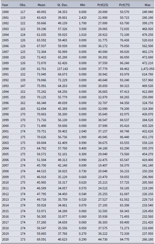
Note: The number of observations corresponds to the number of countries in the IMF’s historical public debt database (Ali Abbas et al. Reference Ali Abbas, Belhocine, El-Ganainy and Horton2011).
2.2 Double Pareto-Lognormal (dPLN)
Let $X$
represent a random variable for the debt-to-GDP ratio, with its outcome denoted by
$X$
represent a random variable for the debt-to-GDP ratio, with its outcome denoted by $x$
, where
$x$
, where $x\gt 0$
. The probability density function of the dPLN is given by
$x\gt 0$
. The probability density function of the dPLN is given by
 \begin{eqnarray} f_{\text{dPLN}}(x; \mu,\sigma,\alpha,\beta) &=&\frac {\alpha \beta }{\alpha + \beta }\left [ x^{- \alpha - 1}\exp \left ( \alpha \mu + \frac {\alpha ^{2}\sigma ^{2}}{2}\right) \Phi \left ( \frac {\log (x) - \mu - \alpha \sigma ^{2}}{\sigma }\right) \right. \\\nonumber && + \left. x^{\beta - 1}\exp \left ( - \beta \mu + \frac {\beta ^{2}\sigma ^{2}}{2}\right) \left ( 1 - \Phi \left ( \frac {\log (x) - \mu + \beta \sigma ^{2}}{\sigma }\right) \right) \right], \end{eqnarray}
where $\Phi (\cdot)$
is the cumulative distribution function of the standard normal distribution. The dPLN has four parameters:
$\Phi (\cdot)$
is the cumulative distribution function of the standard normal distribution. The dPLN has four parameters: $\mu,\sigma$
are the mean and standard deviation of the lognormal component, and
$\mu,\sigma$
are the mean and standard deviation of the lognormal component, and $\alpha,\beta \gt 0$
are the power law (Pareto) exponents for the upper and lower tails, respectively.Footnote 3
$\alpha,\beta \gt 0$
are the power law (Pareto) exponents for the upper and lower tails, respectively.Footnote 3
Similar to the Pareto distribution, the dPLN has finitely many moments, a feature of empirical relevance (Kocherlakota, Reference Kocherlakota1997; Toda and Walsh, Reference Toda and Walsh2015). Specifically, the $r$
th moment about origin for the dPLN takes the following form:
$r$
th moment about origin for the dPLN takes the following form:
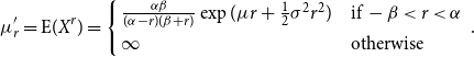 \begin{eqnarray} \mu _r^{\prime} = \text{E}(X^r) = \left \{ \begin{array}{l@{\quad}l} \frac {\alpha \beta }{(\alpha - r)(\beta + r)} \exp (\mu r + \frac {1}{2}\sigma ^2 r^2) & \text{if } -\beta \lt r \lt \alpha \\ \infty & \text{otherwise} \end{array} \right. {.} \end{eqnarray}
This implies that $\mu _r^{\prime}$
does not exist for
$\mu _r^{\prime}$
does not exist for $r \geq \alpha$
. For instance, the variance exists only if the upper-tail power law exponent satisfies
$r \geq \alpha$
. For instance, the variance exists only if the upper-tail power law exponent satisfies $\alpha \gt 2$
.
$\alpha \gt 2$
.
There are several features of the dPLN that make the distribution attractive for computational works. First, similar to the lognormal and Pareto distributions, the dPLN is analytically tractable (Reed, Reference Reed2003; Reed and Jorgensen, Reference Reed and Jorgensen2004), as its moments generally have closed-form expressions. Second, the dPLN is flexible, capturing the lognormal and double Pareto distributions as limiting cases (for $\alpha,\beta \rightarrow \infty$
and
$\alpha,\beta \rightarrow \infty$
and $\sigma \rightarrow 0$
, respectively). Third, the distribution is parsimonious, with only three (
$\sigma \rightarrow 0$
, respectively). Third, the distribution is parsimonious, with only three ( $\alpha =\beta$
) or four (
$\alpha =\beta$
) or four ( $\alpha \ne \beta$
) parameters. Fourth, the dPLN allows for fat tails, making it convenient for modeling heavy-tailed data compared to other, more complex mixture distributions. Fifth, since
$\alpha \ne \beta$
) parameters. Fourth, the dPLN allows for fat tails, making it convenient for modeling heavy-tailed data compared to other, more complex mixture distributions. Fifth, since $\alpha, \beta$
describe the concentration at the top and bottom of the distribution, respectively, they can be used in applied work to decompose inequality at the top and bottom of the size distribution (Toda, Reference Toda2012, Reference Toda2014).
$\alpha, \beta$
describe the concentration at the top and bottom of the distribution, respectively, they can be used in applied work to decompose inequality at the top and bottom of the size distribution (Toda, Reference Toda2012, Reference Toda2014).
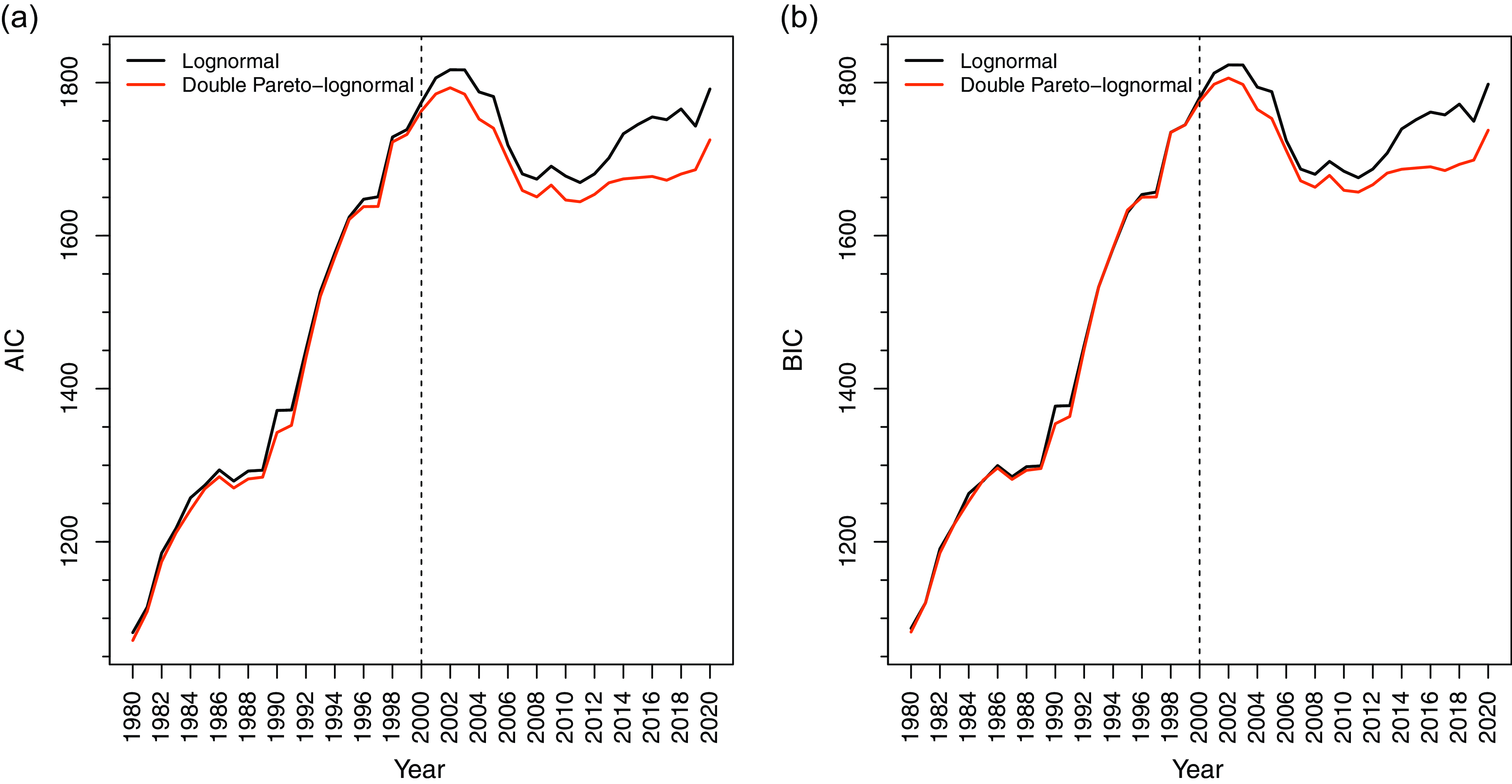
Figure 1. Relative quality of lognormal and dPLN in fitting the debt-to-GDP ratio, 1980–2020.
2.3 Diagnostics
To assess the relative quality of alternative models, we report the log-likelihood, Akaike information criterion (AIC), and Bayesian information criterion (BIC). While both AIC and BIC account for overfitting, BIC penalizes the number of model parameters more heavily than AIC. Generally, the model with the lowest AIC or BIC is preferred.
To evaluate the goodness of fit of individual models, we also perform the Kolmogorov–Smirnov (KS) and Anderson–Darling (AD) tests, and produce quantile–quantile (Q–Q) and distributional plots. The KS and AD tests, commonly used in the size distribution literature (e.g., Toda, Reference Toda2017), compare the empirical distribution with that of a fitted model. The AD test is more robust than the KS test to deviations in the tails, which makes it more relevant for the analysis of tail heaviness. The KS and AD p-values formally test the null hypothesis that the sample is drawn from the fitted distribution.
3. Results
3.1 Lognormal vs. dPLN
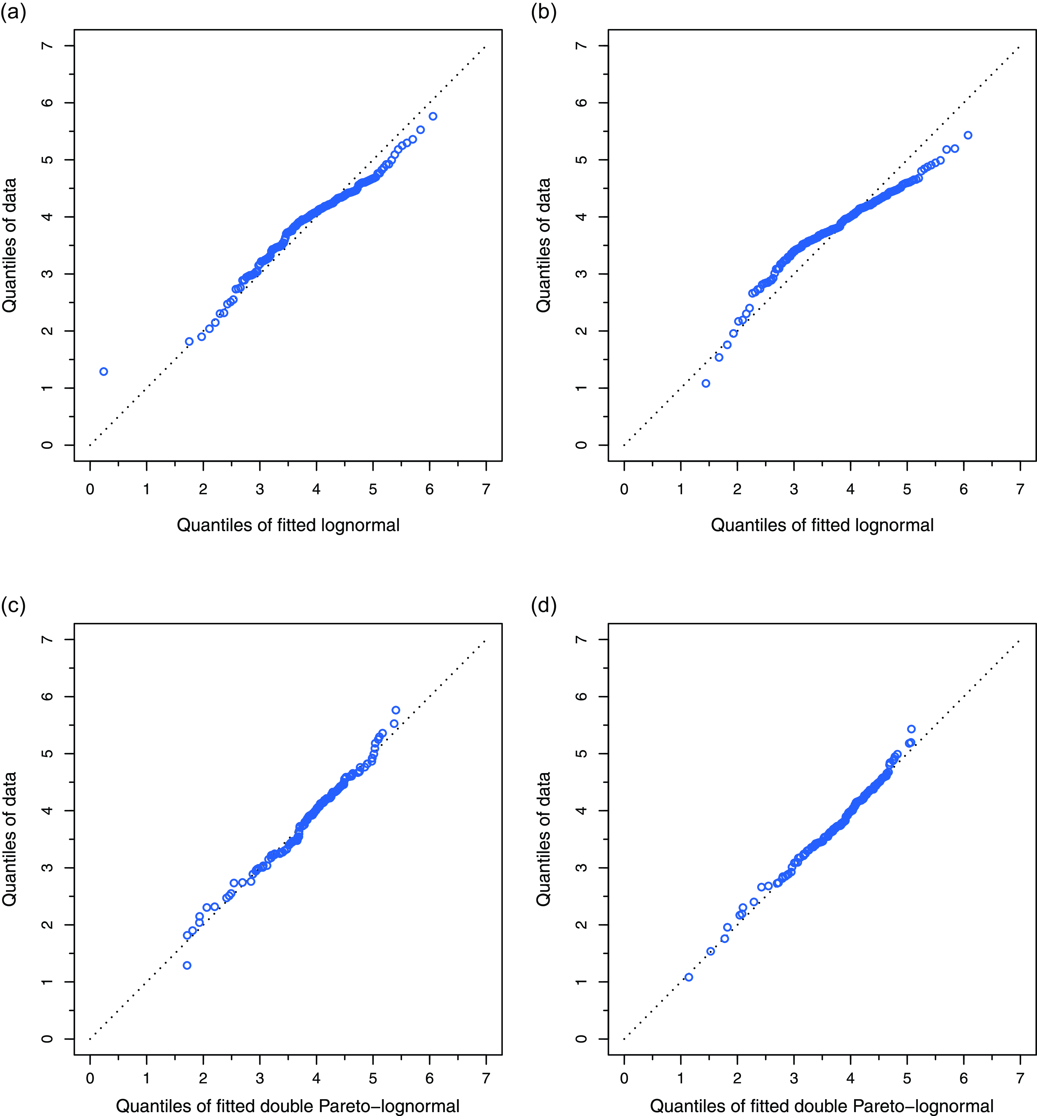
Figure 2. Q–Q plots of fitted lognormal and dPLN: (a) lognormal fit for 1997; (b) lognormal fit for 2015; (c) dPLN fit for 1997; (d) dPLN fit for 2015.
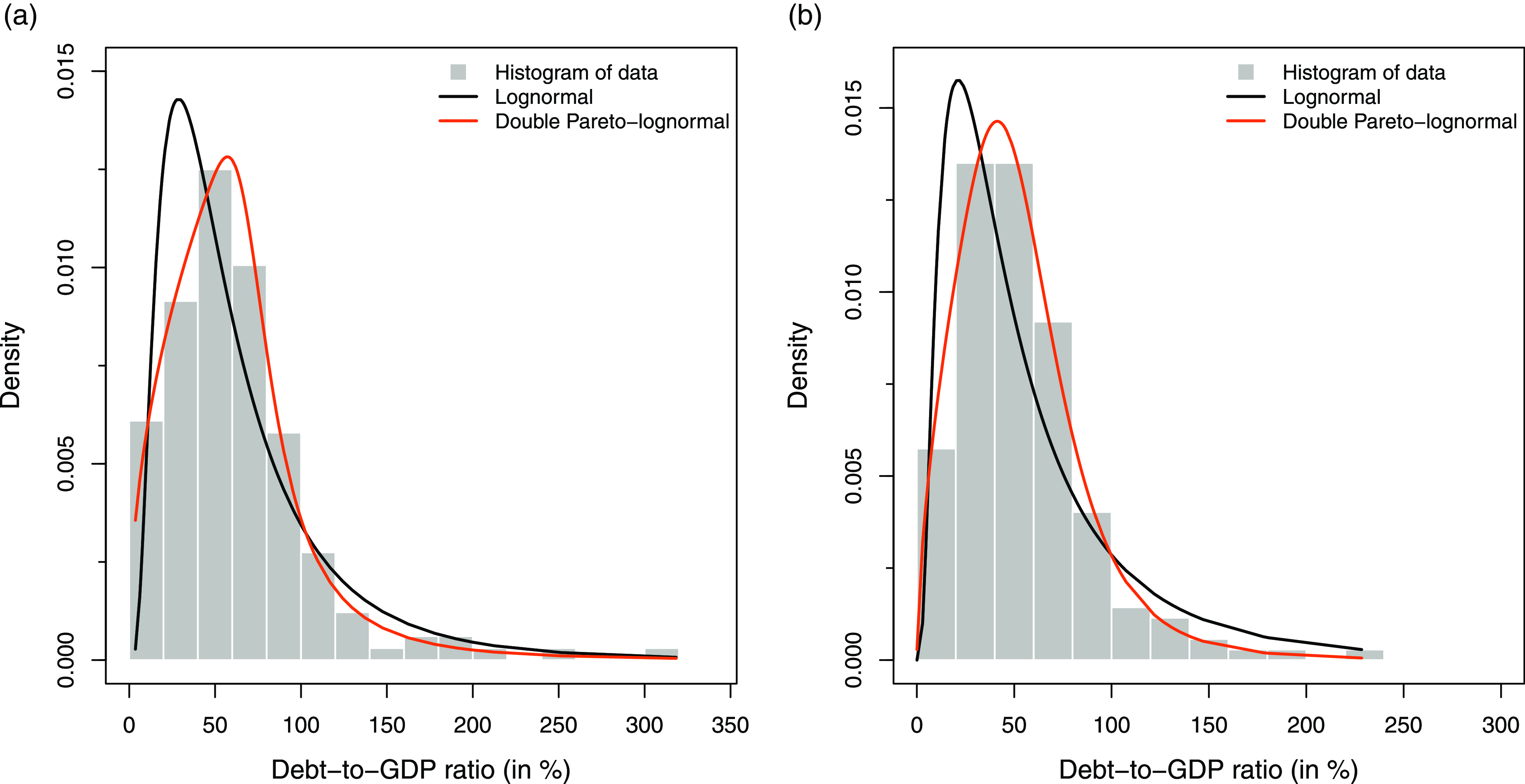
Figure 3. Histogram of data and density plots of fitted lognormal and dPLN: (a) densities for 1997; (b) densities for 2015.
Figure 1 summarizes the relative quality of the lognormal and dPLN distributions in fitting the debt-to-GDP ratio for the period between 1980 and 2020.Footnote 4 According to both AIC and, particularly, BIC, the performances of the two distributions are largely comparable during 1980–2000, though dPLN exhibits a slight edge over the lognormal. After 2000, however, the performances diverge significantly, with dPLN starkly outperforming the lognormal.
The goodness-of-fit test results support the plausibility of dPLN. The KS and AD tests do not reject dPLN at the 0.05 significance level in 40 and 41, respectively, out of 41 years, whereas the lognormal is not rejected in 28 years, 20 of which are before 2000. This indicates that dPLN performs at least as well as the lognormal before 2000, but post-2000, dPLN’s performance remains strong while the lognormal’s performance deteriorates.
Visual evidence for this can be found in Figures 2 and 3, which compare the fits of the two distributions to data from before and after 2000, using 1997 and 2015 as examples. From Q–Q plots in Figure 2, it is apparent that the lognormal fit to 1997 data (panel (a)) is fairly good, with only a small deviation in the upper tail. However, for the 2015 data (panel (b)), there are significant departures in both the upper and lower quantiles of the fitted lognormal distribution. On the other hand, dPLN’s quantiles align closely with the data in both years (panels (c) and (d)). Figure 3 further illuminates this with density plots, where again one observes the striking fit of dPLN to the debt-to-GDP ratio.
Overall, both model fit criteria and goodness-of-fit tests strongly favor dPLN over the lognormal.
Figure 4 shows the MLE estimates of the dPLN parameters for each year. Several salient observations come to light. First, the upper-tail power law exponent $\alpha$
hovers around 2.5, with an average of 2.76 across all years. The lower-tail power law exponent
$\alpha$
hovers around 2.5, with an average of 2.76 across all years. The lower-tail power law exponent $\beta$
has an average of 1.63 across all years.Footnote 5 Econometrically, this suggests the tail heaviness of government debt, which explains the lognormal’s poor fit in figures 2 and 3. Economically, this suggests concentration at the top and bottom of the distribution, which has implications for inequality and policy design. Second, for
$\beta$
has an average of 1.63 across all years.Footnote 5 Econometrically, this suggests the tail heaviness of government debt, which explains the lognormal’s poor fit in figures 2 and 3. Economically, this suggests concentration at the top and bottom of the distribution, which has implications for inequality and policy design. Second, for $\alpha \approx 2.76$
and
$\alpha \approx 2.76$
and $r \lt \alpha$
, only the first and second moments (i.e., mean and variance, respectively) exist for the debt-to-GDP ratio. This is instructive for descriptive and empirical analysis (e.g., GMM) of government debt. Third, the log variance parameter
$r \lt \alpha$
, only the first and second moments (i.e., mean and variance, respectively) exist for the debt-to-GDP ratio. This is instructive for descriptive and empirical analysis (e.g., GMM) of government debt. Third, the log variance parameter $\sigma$
remains generally stable, with an average of 0.28 across all years. This further illustrates the implausibility of the lognormal distribution and its theoretical basis, as under a pure random multiplicative growth mechanism, the size distribution would be lognormal, with an increasing variance over time. For the debt-to-GDP ratio, we find a lack of support for this to be the case.
$\sigma$
remains generally stable, with an average of 0.28 across all years. This further illustrates the implausibility of the lognormal distribution and its theoretical basis, as under a pure random multiplicative growth mechanism, the size distribution would be lognormal, with an increasing variance over time. For the debt-to-GDP ratio, we find a lack of support for this to be the case.

Figure 4. DPLN parameter estimates: (a) upper-tail power law exponent $\alpha$
; (b) lower-tail power law exponent
$\alpha$
; (b) lower-tail power law exponent $\beta$
; (c) log variance parameter
$\beta$
; (c) log variance parameter $\sigma$
.
$\sigma$
.
3.2 Other Candidate Distributions
To compare the performance of dPLN within a broader class of parametric distributions, we consider two additional flexible distributions with varying tail heaviness: first, generalized beta II (Toda, Reference Toda2017), and second, Pareto-tails lognormal (PTLN) (Luckstead and Devadoss, Reference Luckstead and Devadoss2017).
The generalized beta II is a four-parameter distribution that nests many common distributions, including exponential, (generalized) gamma, lognormal, Weibull, chi-square, Lomax, Rayleigh, Laplace, and log-logistic, among others. The PTLN is a close alternative to dPLN and shares many of its attractive features but has six parameters: in addition to the four parameters of dPLN, PTLN includes $\tau _{l}$
and
$\tau _{l}$
and $\tau _{u}$
, which are the transition (threshold) points from the lower tail Pareto to the lognormal body and from the lognormal body to the upper tail Pareto, respectively. PTLN also nests the lognormal-upper tail Pareto distribution of Ioannides and Skouras (Reference Ioannides and Skouras2013) (for
$\tau _{u}$
, which are the transition (threshold) points from the lower tail Pareto to the lognormal body and from the lognormal body to the upper tail Pareto, respectively. PTLN also nests the lognormal-upper tail Pareto distribution of Ioannides and Skouras (Reference Ioannides and Skouras2013) (for $\tau _{l}=x_{\min }$
).
$\tau _{l}=x_{\min }$
).
The relative quality of these distributions is presented in Figure 5.Footnote 6 Evidently, both AIC and BIC favor dPLN. The generalized beta II does not perform as well as the dPLN, with the KS and AD tests failing to reject the distribution in 11 and 35, respectively, out of 41 years. Therefore, dPLN remains dominant among a large class of parametric distributions. However, PTLN is a close contender. The additional two parameters in PTLN improve its AIC performance compared to dPLN, but not its BIC performance, as expected. The KS and AD tests do not reject PTLN for any of the years analyzed, indicating that PTLN fits the government debt data quite well, though it is less parsimonious and less tractable than dPLN.
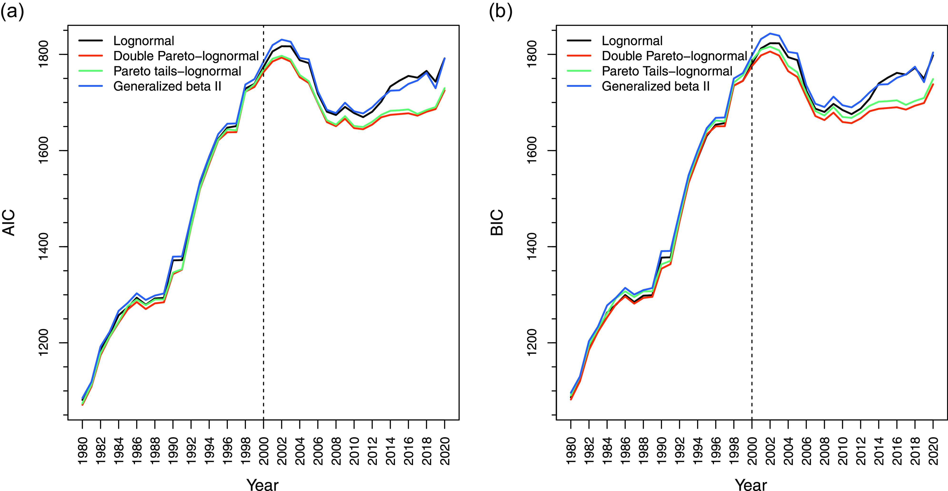
Figure 5. Relative quality of alternative distributions in fitting the debt-to-GDP ratio, 1980–2020.
Taken together, the analytical tractability, flexibility, and parsimony of dPLN, along with its remarkable performance in terms of model fit criteria and goodness-of-fit tests, rightfully validate the distribution as one of the benchmarks for fitting the debt-to-GDP ratio.
Supplementary material
The supplementary material for this article can be found at https://doi.org/10.1017/S1365100525000276.


 Open access