


1. Introduction
1.1. The problem
Consider an urn containing n balls, each ball having one of $c\geq 2$
different colors, and suppose we draw out
$c\geq 2$
different colors, and suppose we draw out $k\leq n$
of them. We will compare the difference in sampling with and without replacement. Write
$k\leq n$
of them. We will compare the difference in sampling with and without replacement. Write ${\boldsymbol{\ell}} = (\ell_1,\ell_2, \ldots, \ell_c)$
for the vector representing the number of balls of each color in the urn, so that there are
${\boldsymbol{\ell}} = (\ell_1,\ell_2, \ldots, \ell_c)$
for the vector representing the number of balls of each color in the urn, so that there are $\ell_i$
balls of color i,
$\ell_i$
balls of color i, $1\leq i\leq c$
, and
$1\leq i\leq c$
, and $\ell_1+\ell_2+\cdots+\ell_c = n$
. Write
$\ell_1+\ell_2+\cdots+\ell_c = n$
. Write ${\boldsymbol{s}} = (s_1,s_2, \ldots, s_c)$
for the number of balls of each color drawn out, so that
${\boldsymbol{s}} = (s_1,s_2, \ldots, s_c)$
for the number of balls of each color drawn out, so that $s_1+s_2+\cdots+s_c = k$
.
$s_1+s_2+\cdots+s_c = k$
.
When sampling without replacement, the probability that the colors of the k balls drawn are given by ${\boldsymbol{s}}$
is given by the multivariate hypergeometric probability mass function (p.m.f.)
${\boldsymbol{s}}$
is given by the multivariate hypergeometric probability mass function (p.m.f.)
 \begin{equation}H(n,k, {\boldsymbol{\ell}};\,{\boldsymbol{s}})\,:\!=\, \frac{ \prod_{i=1}^c \binom{\ell_i}{s_i}}{\binom{n}{k}} =\frac{ \binom{k}{{\boldsymbol{s}}} \binom{n-k}{{\boldsymbol{\ell}}- {\boldsymbol{s}}}}{\binom{n}{{\boldsymbol{\ell}}}},\end{equation}
for all ${\boldsymbol{s}}$
with
${\boldsymbol{s}}$
with $0\leq s_i\leq\ell_i$
for all i, and
$0\leq s_i\leq\ell_i$
for all i, and $s_1+\cdots+s_c=k$
. In (1) and throughout, we write
$s_1+\cdots+s_c=k$
. In (1) and throughout, we write $\binom{v}{{\boldsymbol{u}}} = v!/\prod_{i=1}^c u_i!$
for the multinomial coefficient for any vector
$\binom{v}{{\boldsymbol{u}}} = v!/\prod_{i=1}^c u_i!$
for the multinomial coefficient for any vector ${\boldsymbol{u}}=(u_1,\ldots,u_c)$
with
${\boldsymbol{u}}=(u_1,\ldots,u_c)$
with $u_1+\cdots+u_c = v$
.
$u_1+\cdots+u_c = v$
.
Our goal is to compare $H(n,k, {\boldsymbol{\ell}};\, {\boldsymbol{s}})$
with the corresponding p.m.f.
$H(n,k, {\boldsymbol{\ell}};\, {\boldsymbol{s}})$
with the corresponding p.m.f. $B(n, k, {\boldsymbol{\ell}};\, {\boldsymbol{s}})$
of sampling with replacement, which is given by the multinomial distribution p.m.f.
$B(n, k, {\boldsymbol{\ell}};\, {\boldsymbol{s}})$
of sampling with replacement, which is given by the multinomial distribution p.m.f.
 \begin{equation}B(n, k, {\boldsymbol{\ell}};\, {\boldsymbol{s}})\,:\!=\, \binom{k}{{\boldsymbol{s}}} \prod_{i=1}^c \bigg( \frac{\ell_i}{n} \bigg)^{s_i}\end{equation}
for all ${\boldsymbol{s}}$
with
${\boldsymbol{s}}$
with $s_i\geq 0$
and
$s_i\geq 0$
and $s_1+\cdots+s_c=k$
.
$s_1+\cdots+s_c=k$
.
The study of the relationship between sampling with and without replacement has a long history and numerous applications in both statistics and probability; see, e.g., the classic review in [Reference Rao22], or [Reference Thompson24]. Beyond the elementary observation that B and H have the same mean, namely that $\sum_{{\boldsymbol{s}}} B(n,k,{\boldsymbol{\ell}};\, {\boldsymbol{s}}) s_i=\sum_{{\boldsymbol{s}}} H(n,k,{\boldsymbol{\ell}};\, {\boldsymbol{s}}) s_i = k \ell_i/n$
for each i, it is well known that in certain limiting regimes the p.m.f.s themselves are close in a variety of senses. For example, [Reference Diaconis and Freedman12, Theorem 4] showed that H and B are close in the total variation distance
$\sum_{{\boldsymbol{s}}} B(n,k,{\boldsymbol{\ell}};\, {\boldsymbol{s}}) s_i=\sum_{{\boldsymbol{s}}} H(n,k,{\boldsymbol{\ell}};\, {\boldsymbol{s}}) s_i = k \ell_i/n$
for each i, it is well known that in certain limiting regimes the p.m.f.s themselves are close in a variety of senses. For example, [Reference Diaconis and Freedman12, Theorem 4] showed that H and B are close in the total variation distance $\| P-Q \| \,:\!=\, \sup_A |P(A) - Q(A)|$
:
$\| P-Q \| \,:\!=\, \sup_A |P(A) - Q(A)|$
:
 \begin{equation}\|H(n,k, {\boldsymbol{\ell}};\, \cdot)-B(n,k, {\boldsymbol{\ell}};\, \cdot)\| \leq \frac{ck}{n}.\end{equation}
In this paper we give bounds on the relative entropy (or Kullback–Leibler divergence) between H and B, which for brevity we denote as
 \begin{equation}D(n,k, {\boldsymbol{\ell}}) \,:\!=\,D ( H(n,k, {\boldsymbol{\ell}};\, \cdot)\,\|\,B(n,k, {\boldsymbol{\ell}};\, \cdot)) =\sum_{{\boldsymbol{s}}} H(n,k, {\boldsymbol{\ell}};\, {\boldsymbol{s}}) \log \bigg(\frac{ H(n,k, {\boldsymbol{\ell}};\, {\boldsymbol{s}})}{B(n,k, {\boldsymbol{\ell}};\, {\boldsymbol{s}})} \bigg).\end{equation}
[All logarithms are natural logarithms to base e.] Clearly, if $\ell_r = 0$
for some r, then bounding
$\ell_r = 0$
for some r, then bounding $D(n,k;{\boldsymbol{\ell}})$
becomes equivalent to the same problem with a smaller number of colors c, so we may assume that each
$D(n,k;{\boldsymbol{\ell}})$
becomes equivalent to the same problem with a smaller number of colors c, so we may assume that each $\ell_r \geq 1$
for simplicity.
$\ell_r \geq 1$
for simplicity.
Interest in controlling the relative entropy derives in part from the fact that it naturally arises in many core statistical problems, e.g. as the optimal hypothesis testing error exponent in Stein’s lemma; see, e.g., [Reference Cover and Thomas9, Theorem 12.8.1]. Further, bounding the relative entropy also provides control of the distance between H and B in other senses. For example, Pinsker’s inequality, e.g. [Reference Tsybakov26, Lemma 2.9.1], states that, for any two p.m.f.s P and Q,
 \begin{equation}2\| P - Q \|^2 \leq D(P\,\|\,Q),\end{equation}
while the Bretagnolle–Huber bound [Reference Bretagnolle and Huber7, Reference Canonne8] gives $\| P - Q \|^2 \leq 1 - \exp\{-D(P\,\|\,Q)\}$
.
$\| P - Q \|^2 \leq 1 - \exp\{-D(P\,\|\,Q)\}$
.
Our results also follow a long line of work that has been devoted to establishing probabilistic theorems in terms of relative entropy. Information-theoretic arguments often provide insights into the underlying reasons why the result at hand holds. Among many others, examples include the well-known work of [Reference Barron4] on the information-theoretic central limit theorem; information-theoretic proofs of Poisson convergence and Poisson approximation [Reference Kontoyiannis, Harremoës and Johnson20]; compound Poisson approximation bounds [Reference Barbour, Johnson, Kontoyiannis and Madiman3]; convergence to Haar measure on compact groups [Reference Harremoës16]; connections with extreme value theory [Reference Johnson18]; and the discrete central limit theorem [Reference Gavalakis and Kontoyiannis15]. We refer to [Reference Gavalakis and Kontoyiannis14] for a detailed review of this line of work.
The relative entropy in (4) has been studied before. Stam [23] established the bound
 \begin{equation} D ( n,k, {\boldsymbol{\ell}}) \leq \frac{(c-1) k(k-1)}{2(n-1)(n-k+1)}\end{equation}
uniformly in ${\boldsymbol{\ell}}$
, and also provided an asymptotically matching lower bound,
${\boldsymbol{\ell}}$
, and also provided an asymptotically matching lower bound,
 \begin{equation}D( n,k, {\boldsymbol{\ell}} ) \geq \frac{(c-1) k(k-1)}{4(n-1)^2},\end{equation}
indicating that, in the regime $k=o(n)$
and fixed c, the relative entropy
$k=o(n)$
and fixed c, the relative entropy $D ( n,k, {\boldsymbol{\ell}} )$
is of order
$D ( n,k, {\boldsymbol{\ell}} )$
is of order $(c-1) k^2/2n^2$
.
$(c-1) k^2/2n^2$
.
More recently, related bounds were established by [Reference Harremoës and Matúš17], showing that (see [Reference Harremoës and Matúš17, Theorem 4.5])
 \begin{equation} D( n,k, {\boldsymbol{\ell}}) \leq (c-1) \bigg(\log\bigg( \frac{n-1}{n-k} \bigg) - \frac{k}{n} + \frac{1}{n-k+1} \bigg),\end{equation}
and (see [Reference Harremoës and Matúš17, Theorem 4.4])
 \begin{equation} D( n,k, {\boldsymbol{\ell}}) \geq \frac{(c-1)}{2}( r - 1 - \ln r) \quad\mbox{for } r = \frac{n-k+1}{n-1},\end{equation}
both results also holding uniformly in ${\boldsymbol{\ell}}$
. Moreover, in the regime where
${\boldsymbol{\ell}}$
. Moreover, in the regime where $k/n \rightarrow s$
and
$k/n \rightarrow s$
and $0 < \epsilon \leq \ell_r/n$
for all r, [Reference Harremoës and Matúš17] showed that the lower bound in (9) is asymptotically sharp and the upper bound in (8) is sharp to within a factor of two by proving that
$0 < \epsilon \leq \ell_r/n$
for all r, [Reference Harremoës and Matúš17] showed that the lower bound in (9) is asymptotically sharp and the upper bound in (8) is sharp to within a factor of two by proving that
 \begin{equation}\lim_{n \rightarrow \infty} D( n,k, {\boldsymbol{\ell}} ) =\frac{c-1}{2}\bigg({-}\log(1-s) -s \bigg) \approx(c-1) \bigg( \frac{s^2}{4} + \frac{s^3}{6} \bigg).\end{equation}
1.2. Main results
Despite the fact that (6) and (8) are both asymptotically optimal in the sense described above, it turns out it is possible to obtain more accurate upper bounds on $D(n,k,{\boldsymbol{\ell}})$
if we allow them to depend on
$D(n,k,{\boldsymbol{\ell}})$
if we allow them to depend on ${\boldsymbol{\ell}}$
. Indeed, as remarked in [Reference Harremoës and Matúš17], ‘a good upper bound should depend on
${\boldsymbol{\ell}}$
. Indeed, as remarked in [Reference Harremoës and Matúš17], ‘a good upper bound should depend on ${\boldsymbol{\ell}}$
” (in our notation). In this vein, our main result is the following; it is proved in Section 2.2.
${\boldsymbol{\ell}}$
” (in our notation). In this vein, our main result is the following; it is proved in Section 2.2.
Theorem 1. For any $1\leq k \leq n/2$
,
$1\leq k \leq n/2$
, $c\geq 2$
, and
$c\geq 2$
, and ${\boldsymbol{\ell}}=(\ell_1,\cdots,\ell_c)$
with
${\boldsymbol{\ell}}=(\ell_1,\cdots,\ell_c)$
with $\ell_1+\cdots+\ell_c=n$
and
$\ell_1+\cdots+\ell_c=n$
and $\ell_r\geq 1$
for each r, the relative entropy
$\ell_r\geq 1$
for each r, the relative entropy $D(n,k,{\boldsymbol{\ell}})$
between H and B satisfies
$D(n,k,{\boldsymbol{\ell}})$
between H and B satisfies
 \begin{align} D(n,k, {\boldsymbol{\ell}}) & \leq \frac{c-1}{2}\bigg(\log\bigg(\frac{n}{n-k}\bigg) - \frac{k}{n-1}\bigg) \nonumber \\ & \quad + \frac{k(2n+1)}{12n(n-1)(n-k)}\sum_{i=1}^c\frac{n}{\ell_i} + \frac{1}{360}\bigg(\frac{1}{(n-k)^3} - \frac{1}{n^3}\bigg)\sum_{i=1}^c\frac{n^3}{\ell_i^3}. \end{align}
While the bound of Theorem 1 is simple, straightforward, and works well for the balanced cases described below, it is least accurate in the case of small $\ell_i$
; see Figure 1. We therefore also provide an alternative expression in Proposition 1. For simplicity, we only give the result in the case
$\ell_i$
; see Figure 1. We therefore also provide an alternative expression in Proposition 1. For simplicity, we only give the result in the case $c=2$
, though similar arguments will work in general, see Remark 6. It is proved in Section 3.
$c=2$
, though similar arguments will work in general, see Remark 6. It is proved in Section 3.

Figure 1. Comparison of the true values of $D(100,30,(\ell,100-\ell))$
, plotted as circles, with the uniform upper bounds in (6), (8), and the uniform lower bound (9), all plotted as straight lines, and also with the new bounds in Theorem 1 (dashed line) and Proposition 1 (dotted line). The combination of the two new bounds outperforms those of [Reference Harremoës and Matúš17, 23] for the whole range of the values of
$D(100,30,(\ell,100-\ell))$
, plotted as circles, with the uniform upper bounds in (6), (8), and the uniform lower bound (9), all plotted as straight lines, and also with the new bounds in Theorem 1 (dashed line) and Proposition 1 (dotted line). The combination of the two new bounds outperforms those of [Reference Harremoës and Matúš17, 23] for the whole range of the values of $\ell$
in this case.
$\ell$
in this case.
Proposition 1. Under the assumptions of Theorem 1, if $c=2$
and
$c=2$
and $\ell \leq n/2$
,
$\ell \leq n/2$
,
 \begin{align*} D(n,k,(\ell,n-\ell)) & \leq \ell\bigg[\bigg(1-\frac{k}{n}\bigg)\log\bigg(1-\frac{k}{n}\bigg) + \frac{k}{n} - \frac{k}{2n(n-1)} \bigg] \\ & \quad + \frac{k\ell}{(n-1)(n-\ell)(n-k)} \\ & \quad - \frac{k(k-1)}{2n(n-1)}\ell(\ell-1)\log\bigg(\frac{\ell}{\ell-1}\bigg) \\ & \quad - \frac{k(k-1)(k-2)}{6n(n-1)(n-2)}\ell(\ell-1)(\ell-2) \log\bigg(\frac{(\ell-1)^2}{\ell(\ell-2)}\bigg). \end{align*}
Figure 1 shows a comparison of the earlier uniform bounds (6), (7), and (8) with the new bounds in Theorem 1 and Proposition 1 for the case $n=100$
,
$n=100$
, $k=30$
, and
$k=30$
, and ${\boldsymbol{\ell}}=(\ell,1-\ell)$
, for
${\boldsymbol{\ell}}=(\ell,1-\ell)$
, for $1\leq\ell\leq 50$
. It can be seen that the combination of the two new upper bounds outperforms the earlier ones over the entire range of values considered.
$1\leq\ell\leq 50$
. It can be seen that the combination of the two new upper bounds outperforms the earlier ones over the entire range of values considered.
Remark 1. The dependence of the bound (11) in Theorem 1 on ${\boldsymbol{\ell}}$
is only via the quantities
${\boldsymbol{\ell}}$
is only via the quantities
 \begin{equation} \Sigma_1(n,c,{\boldsymbol{\ell}})\,:\!=\,\sum_{r=1}^c \frac{n}{\ell_r}, \qquad \Sigma_2(n,c,{\boldsymbol{\ell}})\,:\!=\,\sum_{r=1}^c \frac{n^3}{\ell_r^3}.\end{equation}
For $\Sigma_1$
, in the ‘balanced’ case where each
$\Sigma_1$
, in the ‘balanced’ case where each $\ell_r = n/c$
, we have
$\ell_r = n/c$
, we have $\Sigma_1(n,c,{\boldsymbol{\ell}})= c^2$
, and using Jensen’s inequality it is easy to see that we always have
$\Sigma_1(n,c,{\boldsymbol{\ell}})= c^2$
, and using Jensen’s inequality it is easy to see that we always have $\Sigma_1(n,c,{\boldsymbol{\ell}})\geq c^2$
. In fact, the Schur–Ostrowski criterion shows that (12) is Schur convex, and hence respects the majorization order, being largest in ‘unbalanced’ cases. For example, if
$\Sigma_1(n,c,{\boldsymbol{\ell}})\geq c^2$
. In fact, the Schur–Ostrowski criterion shows that (12) is Schur convex, and hence respects the majorization order, being largest in ‘unbalanced’ cases. For example, if $\ell_1 = \cdots = \ell_{c-1} = 1$
and
$\ell_1 = \cdots = \ell_{c-1} = 1$
and $\ell_c = n-c+1$
, then
$\ell_c = n-c+1$
, then $\Sigma_1(n,c,{\boldsymbol{\ell}})=(c-1) n + 1/(n-c+1) \sim n(c-1)\to\infty$
as
$\Sigma_1(n,c,{\boldsymbol{\ell}})=(c-1) n + 1/(n-c+1) \sim n(c-1)\to\infty$
as $n \rightarrow \infty$
. On the other hand, in the regime considered in [Reference Harremoës and Matúš17] where all
$n \rightarrow \infty$
. On the other hand, in the regime considered in [Reference Harremoës and Matúš17] where all $\ell_r \geq \epsilon n$
for some
$\ell_r \geq \epsilon n$
for some $0 < \epsilon \leq 1/c$
, we have
$0 < \epsilon \leq 1/c$
, we have $\Sigma_1(n,c,{\boldsymbol{\ell}}) \leq c/\epsilon$
, which is bounded in n.
$\Sigma_1(n,c,{\boldsymbol{\ell}}) \leq c/\epsilon$
, which is bounded in n.
Similar comments apply to $\Sigma_2(n,c,{\boldsymbol{\ell}})$
: it is bounded in balanced cases, including the scenario of [Reference Harremoës and Matúš17], but can grow like
$\Sigma_2(n,c,{\boldsymbol{\ell}})$
: it is bounded in balanced cases, including the scenario of [Reference Harremoës and Matúš17], but can grow like $n^3(c-1)$
in the very unbalanced case.
$n^3(c-1)$
in the very unbalanced case.
Remark 2. The first term in the bound (11) of Theorem 1,
 \begin{align*}\frac{c-1}{2}\bigg(\log\bigg(\frac{n}{n-k}\bigg) - \frac{k}{n-1}\bigg),\end{align*}
matches the asymptotic expression in (10), so Theorem 1 may be regarded as a nonasymptotic version version of (10). In particular, (10) is only valid in the asymptotic case where all $\ell_r \geq \epsilon n$
, when, as discussed above,
$\ell_r \geq \epsilon n$
, when, as discussed above, $\Sigma_1(n,c,{\boldsymbol{\ell}})$
is bounded. Therefore, in this balanced case Theorem 1 recovers the asymptotic result of (10).
$\Sigma_1(n,c,{\boldsymbol{\ell}})$
is bounded. Therefore, in this balanced case Theorem 1 recovers the asymptotic result of (10).
Remark 3. Any bound that holds uniformly in ${\boldsymbol{\ell}}$
must hold in particular for the binary
${\boldsymbol{\ell}}$
must hold in particular for the binary $c=2$
case with
$c=2$
case with $\ell_1 = 1$
,
$\ell_1 = 1$
, $\ell_2=n-1$
. Then H is Bernoulli with parameter
$\ell_2=n-1$
. Then H is Bernoulli with parameter $k/n$
and B is binomial with parameters k and
$k/n$
and B is binomial with parameters k and $1/n$
, and direct calculation gives the exact expression
$1/n$
, and direct calculation gives the exact expression
 \begin{equation*} D(n,k,(1,n-1)) = \bigg(1-\frac{k}{n}\bigg)\log\bigg(1-\frac{k}{n}\bigg) - k\bigg(1-\frac{1}{n}\bigg)\log\bigg(1-\frac{1}{n}\bigg).\end{equation*}
Taking $n\to\infty$
while
$n\to\infty$
while $k/n \rightarrow s$
for some fixed s, in this unbalanced case where
$k/n \rightarrow s$
for some fixed s, in this unbalanced case where $\ell_1=1$
and
$\ell_1=1$
and $\ell_2=n-1$
, we obtain
$\ell_2=n-1$
, we obtain
 \begin{equation} \lim_{n\rightarrow\infty}D(n,ns,(1,n-1)) = s + (1-s)\log(1-s) \approx \frac{s^2}{2} + \frac{s^3}{6}.\end{equation}
Compared with the analogous limiting expression (10) in the balanced case where $\ell_1,\ell_2$
are both bounded below by
$\ell_1,\ell_2$
are both bounded below by $\epsilon n$
, this suggests that the asymptotic behavior of
$\epsilon n$
, this suggests that the asymptotic behavior of $D(n,k,{\boldsymbol{\ell}})$
in the regime
$D(n,k,{\boldsymbol{\ell}})$
in the regime $k/n\to s$
may vary by a factor of two over different values of
$k/n\to s$
may vary by a factor of two over different values of $\ell$
.
$\ell$
.
Remark 4. Comparing the earlier asymptotic expression (10) with (13) reveals some interesting behavior of $D(n,k, (\ell,n-\ell))$
. There is a unique value
$D(n,k, (\ell,n-\ell))$
. There is a unique value $s^* \approx 0.8834$
such that, for
$s^* \approx 0.8834$
such that, for $s < s^*$
, corresponding to small k, the limiting expression in (13) is larger than that in (10), whereas, for
$s < s^*$
, corresponding to small k, the limiting expression in (13) is larger than that in (10), whereas, for $s > s^*$
, the expression in (10) is larger.
$s > s^*$
, the expression in (10) is larger.
1.3. Finite de Finetti theorems
An interesting and intimate connection was revealed in [Reference Diaconis11, Reference Diaconis and Freedman12] between the problem of comparing sampling with and without replacement and finite versions of de Finetti’s theorem. Recall that de Finetti’s theorem says that the distribution of an infinite collection of exchangeable random variables can be represented as a mixture over independent and identically distributed (i.i.d.) sequences; see, e.g., [Reference Kirsch19] for an elementary proof in the binary case. Although such a representation does not always exist for finite exchangeable sequences, approximate versions are possible: If $(X_1,\ldots,X_n)$
are exchangeable, then the distribution of
$(X_1,\ldots,X_n)$
are exchangeable, then the distribution of $(X_1,\ldots,X_k)$
is close to a mixture of independent sequences as long as k is relatively small compared to n. Indeed, [Reference Diaconis and Freedman12] proved such a finite de Finetti theorem using the sampling bound (3).
$(X_1,\ldots,X_k)$
is close to a mixture of independent sequences as long as k is relatively small compared to n. Indeed, [Reference Diaconis and Freedman12] proved such a finite de Finetti theorem using the sampling bound (3).
Let ${\mathcal{A}}= \{ a_1, \ldots, a_c \}$
be an alphabet of size c, and suppose that the random variables
${\mathcal{A}}= \{ a_1, \ldots, a_c \}$
be an alphabet of size c, and suppose that the random variables ${\boldsymbol{X}}_n = (X_1, \ldots, X_n)$
, with values
${\boldsymbol{X}}_n = (X_1, \ldots, X_n)$
, with values $X_i \in {\mathcal{A}}$
, are exchangeable, that is, the distribution of
$X_i \in {\mathcal{A}}$
, are exchangeable, that is, the distribution of ${\boldsymbol{X}}_n$
is the same as that of
${\boldsymbol{X}}_n$
is the same as that of $(X_{\pi(1)}, \ldots, X_{\pi(n)})$
for any permutation
$(X_{\pi(1)}, \ldots, X_{\pi(n)})$
for any permutation $\pi$
on
$\pi$
on $\{1,\ldots,n\}$
. Given a sequence
$\{1,\ldots,n\}$
. Given a sequence ${\boldsymbol{y}} \in {\mathcal{A}}^m$
of length m, its type
${\boldsymbol{y}} \in {\mathcal{A}}^m$
of length m, its type ${\mathcal T}_m({\boldsymbol{y}})$
[Reference Csiszár10] is the vector of its empirical frequencies: the rth component of
${\mathcal T}_m({\boldsymbol{y}})$
[Reference Csiszár10] is the vector of its empirical frequencies: the rth component of ${\mathcal T}_m({\boldsymbol{y}})$
is
${\mathcal T}_m({\boldsymbol{y}})$
is $({1}/{m})\sum_{i=1}^m\mathbf{1}(y_i = a_r)$
,
$({1}/{m})\sum_{i=1}^m\mathbf{1}(y_i = a_r)$
, $1\leq r\leq c$
. The sequence
$1\leq r\leq c$
. The sequence ${\boldsymbol{X}}_n$
induces a measure
${\boldsymbol{X}}_n$
induces a measure $\mu$
on p.m.f.s
$\mu$
on p.m.f.s ${\boldsymbol{p}}$
on
${\boldsymbol{p}}$
on ${\mathcal{A}}$
via
${\mathcal{A}}$
via
 \begin{equation} \mu({\boldsymbol{p}}) = {\mathbb P}({\mathcal T}_n({\boldsymbol{X}}_n) = {\boldsymbol{p}}).\end{equation}
This is the law of the empirical measure induced by ${\boldsymbol{X}}_n$
on
${\boldsymbol{X}}_n$
on ${\mathcal{A}}$
.
${\mathcal{A}}$
.
For each $1\leq k\leq n$
, let
$1\leq k\leq n$
, let $P_k$
denote the joint p.m.f. of
$P_k$
denote the joint p.m.f. of ${\boldsymbol{X}}_k = (X_1, \ldots, X_k)$
, and write
${\boldsymbol{X}}_k = (X_1, \ldots, X_k)$
, and write
 \begin{equation}M_{k,\mu}({\boldsymbol{z}}) =\int {\boldsymbol{p}}^k({\boldsymbol{z}})\,{\mathrm{d}}\mu({\boldsymbol{p}}),\quad {\boldsymbol{z}}\in{\mathcal{A}}^k,\end{equation}
for the mixture of the i.i.d. distributions ${\boldsymbol{p}}^k$
with respect to the mixing measure
${\boldsymbol{p}}^k$
with respect to the mixing measure $\mu$
. A key step in the connection between sampling bounds and finite de Finetti theorems is the simple observation that, given that its type
$\mu$
. A key step in the connection between sampling bounds and finite de Finetti theorems is the simple observation that, given that its type ${\mathcal T}_k({\boldsymbol{X}}_k)={\boldsymbol{q}}$
, the exchangeable sequence
${\mathcal T}_k({\boldsymbol{X}}_k)={\boldsymbol{q}}$
, the exchangeable sequence ${\boldsymbol{X}}_k$
is uniformly distributed on the set of sequences with type
${\boldsymbol{X}}_k$
is uniformly distributed on the set of sequences with type ${\boldsymbol{q}}$
. In other words, for any
${\boldsymbol{q}}$
. In other words, for any ${\boldsymbol{x}}\in{\mathcal{A}}^k$
,
${\boldsymbol{x}}\in{\mathcal{A}}^k$
,
 \begin{equation}P_k({\boldsymbol{x}}) =\frac{1}{ \binom{k}{{\boldsymbol{s}}}}\sum_{{\boldsymbol{p}}} H(n,k, n {\boldsymbol{p}};\, {\boldsymbol{s}}) \mu({\boldsymbol{p}}),\end{equation}
where ${\boldsymbol{s}}=k{\mathcal T}_k({\boldsymbol{x}})$
. This elementary and rather obvious (by symmetry) observation already appears implicitly in the literature, e.g. in [Reference Diaconis11, Reference Gavalakis and Kontoyiannis14].
${\boldsymbol{s}}=k{\mathcal T}_k({\boldsymbol{x}})$
. This elementary and rather obvious (by symmetry) observation already appears implicitly in the literature, e.g. in [Reference Diaconis11, Reference Gavalakis and Kontoyiannis14].
An analogous representation can be easily seen to hold for $M_{k,\mu}$
. Since the probability of an i.i.d. sequence only depends on its type, for any
$M_{k,\mu}$
. Since the probability of an i.i.d. sequence only depends on its type, for any ${\boldsymbol{x}}\in{\mathcal{A}}^k$
we have, with
${\boldsymbol{x}}\in{\mathcal{A}}^k$
we have, with ${\boldsymbol{s}}=k{\mathcal T}_k({\boldsymbol{x}})$
,
${\boldsymbol{s}}=k{\mathcal T}_k({\boldsymbol{x}})$
,
 \begin{equation}M_{k,\mu}({\boldsymbol{x}}) = \frac{1}{ \binom{k}{{\boldsymbol{s}}}}\sum_{{\boldsymbol{p}}} B(n,k, n {\boldsymbol{p}};\, {\boldsymbol{s}}) \mu({\boldsymbol{p}}).\end{equation}
The following simple proposition clarifies the connection between finite de Finetti theorems and sampling bounds. Its proof is a simple consequence of (16) combined with (17) and the log-sum inequality [Reference Cover and Thomas9].
Proposition 2. Suppose ${\boldsymbol{X}}_n=(X_1,\ldots,X_n)$
is a finite exchangeable sequence of random variables with values in
${\boldsymbol{X}}_n=(X_1,\ldots,X_n)$
is a finite exchangeable sequence of random variables with values in ${\mathcal{A}}$
, and let
${\mathcal{A}}$
, and let $\mu$
denote the law of the empirical measure defined by (14). Then, for any
$\mu$
denote the law of the empirical measure defined by (14). Then, for any $k\leq n$
,
$k\leq n$
,
 \begin{equation*} D(P_k\,\|\,M_{k,\mu}) \leq \sum_{{\boldsymbol{p}}}\mu({\boldsymbol{p}})D(n,k,n{\boldsymbol{p}}) \leq \max_{{{\boldsymbol{\ell}}}/{n}\in\mathrm{supp}(\mu)}D(n,k,{\boldsymbol{\ell}}), \end{equation*}
where $M_{k,\mu}$
is the mixture defined in (15) and the maximum is taken over all p.m.f.s of the form
$M_{k,\mu}$
is the mixture defined in (15) and the maximum is taken over all p.m.f.s of the form ${\boldsymbol{\ell}}/n$
in the support of
${\boldsymbol{\ell}}/n$
in the support of $\mu$
.
$\mu$
.
Proof. Fix ${\boldsymbol{s}}$
with
${\boldsymbol{s}}$
with $\sum_{i=1}^c s_i = k$
. The log-sum inequality gives, for any
$\sum_{i=1}^c s_i = k$
. The log-sum inequality gives, for any ${\boldsymbol{x}}$
of type
${\boldsymbol{x}}$
of type ${\mathcal T}_k({\boldsymbol{x}}) = {\boldsymbol{s}}/k$
,
${\mathcal T}_k({\boldsymbol{x}}) = {\boldsymbol{s}}/k$
,
 \begin{align*} P_k({\boldsymbol{x}})\log\bigg(\frac{P_k({\boldsymbol{x}})}{M_{k,\mu}({\boldsymbol{x}})}\bigg) & = \binom{k}{{\boldsymbol{s}}}^{-1} \Bigg(\sum_{{\boldsymbol{p}}}H(n,k,n{\boldsymbol{p}};\,{\boldsymbol{s}})\mu({\boldsymbol{p}})\Bigg) \log\Bigg(\frac{\sum_{{\boldsymbol{p}}}H(n,k,n{\boldsymbol{p}};\,{\boldsymbol{s}})\mu({\boldsymbol{p}})} {\sum_{{\boldsymbol{p}}}B(n,k,n{\boldsymbol{p}};\,{\boldsymbol{s}})\mu({\boldsymbol{p}})}\Bigg) \\ & \leq \binom{k}{{\boldsymbol{s}}}^{-1} \sum_{{\boldsymbol{p}}}\mu({\boldsymbol{p}})H(n,k,n{\boldsymbol{p}};\,{\boldsymbol{s}}) \log\bigg(\frac{H(n,k,n{\boldsymbol{p}};\,{\boldsymbol{s}})} {B(n,k,n{\boldsymbol{p}};\,{\boldsymbol{s}})}\bigg).\end{align*}
Hence, summing over the $\binom{k}{{\boldsymbol{s}}}$
vectors
$\binom{k}{{\boldsymbol{s}}}$
vectors ${\boldsymbol{x}}$
of type
${\boldsymbol{x}}$
of type ${\mathcal T}_k({\boldsymbol{x}}) = {\boldsymbol{s}}/k$
we obtain
${\mathcal T}_k({\boldsymbol{x}}) = {\boldsymbol{s}}/k$
we obtain
 \begin{align*} \sum_{{\boldsymbol{x}}:{\mathcal T}({\boldsymbol{x}})={\boldsymbol{s}}/k}P_k({\boldsymbol{x}}) \log\bigg(\frac{P_k({\boldsymbol{x}})}{M_{k,\mu}({\boldsymbol{x}})}\bigg) \leq \sum_{{\boldsymbol{p}}}\mu({\boldsymbol{p}})H(n,k,n{\boldsymbol{p}};\,{\boldsymbol{s}}) \log\bigg(\frac{H(n,k,n{\boldsymbol{p}};\,{\boldsymbol{s}})}{B(n,k,n{\boldsymbol{p}};\,{\boldsymbol{s}})}\bigg). \end{align*}
Finally, summing over ${\boldsymbol{s}}$
yields
${\boldsymbol{s}}$
yields $D(P_k\,\|\,M_{k,\mu}) \leq \sum_{{\boldsymbol{p}}}\mu({\boldsymbol{p}})D(n,k,n{\boldsymbol{p}})$
, and each of the relative entropy terms can be bounded by the maximum value.
$D(P_k\,\|\,M_{k,\mu}) \leq \sum_{{\boldsymbol{p}}}\mu({\boldsymbol{p}})D(n,k,n{\boldsymbol{p}})$
, and each of the relative entropy terms can be bounded by the maximum value.
Combining Stam’s bound (6) and Proposition 2 immediately gives the following result.
Corollary 1. (Sharp finite de Finetti.) Under the assumptions of Proposition 2, for $1\leq k\leq n$
,
$1\leq k\leq n$
,
 \begin{equation} D(P_k\,\|\,M_{k,\mu}) \leq \frac{(c-1) k(k-1)}{2(n-1)(n-k+1)}. \end{equation}
Pinsker’s inequality (5) and (18) gives
 \begin{equation*} \| P_k - M_{k,\mu} \| \leq \sqrt{\frac{(c-1) k(k-1)}{2(n-1)(n-k+1)}}.\end{equation*}
In the $k=o(n)$
regime this is in fact optimal, in that it is of the same order as the bound in [Reference Diaconis and Freedman12],
$k=o(n)$
regime this is in fact optimal, in that it is of the same order as the bound in [Reference Diaconis and Freedman12],
 \begin{equation} \| P_k - M_{k,\mu} \| \leq \frac{ c k}{n},\end{equation}
which was shown to be of optimal order in k and n when $k=o(n)$
.
$k=o(n)$
.
For certain applications, for example to approximation schemes for minimization of specific polynomials [Reference Berta, Borderi, Fawzi and Scholz5], the dependence on the alphabet size is also of interest; see also [Reference Berta, Gavalakis and Kontoyiannis6] and the references therein. The lower bound (7) shows that the linear dependence on the alphabet size c is optimal for the sampling problem, in the sense that any upper bound that holds for any c, k, and n must have at least linear dependence on c. However, we do not know whether the linear dependence on the alphabet size c is optimal for the de Finetti problem under optimal rates in k,n.
Information-theoretic proofs of finite de Finetti theorems have lately been developed in [Reference Berta, Gavalakis and Kontoyiannis6, Reference Gavalakis and Kontoyiannis13, Reference Gavalakis and Kontoyiannis14]. In [Reference Gavalakis and Kontoyiannis13], the bound
 \begin{equation} D(P_{k}\,\|\,M_{k,\mu}) \leq \frac{5k^2\log n}{n-k}\end{equation}
was obtained for binary sequences, and in [Reference Gavalakis and Kontoyiannis14] the weaker bound
 \begin{equation}D(P_{k}\,\|\,M_{k,\mu})=O\bigg(\bigg(\frac{k}{\sqrt{n}\,}\bigg)^{1/2}\log{\frac{n}{k}}\bigg)\end{equation}
was established for finite-valued random variables. Finally, the sharper bound
 \begin{equation} D(P_{k}\,\|\,M_{k,\mu}) \leq \frac{k(k-1)}{2(n-k-1)}\log c\end{equation}
was derived in [Reference Berta, Gavalakis and Kontoyiannis6], where random variables with values in abstract spaces were also considered. Although the derivations of (20)–(22) are interesting in that they employ purely information-theoretic ideas and techniques, the actual bounds are of strictly weaker rate than the sharp $O(k^2/n^2)$
rate we obtained in Corollary 1 via sampling bounds.
$O(k^2/n^2)$
rate we obtained in Corollary 1 via sampling bounds.
1.3.1. A question on monotonicity
A significant development in the area of information-theoretic proofs of probabilistic limit theorems was in 2004, when it was shown [Reference Artstein, Ball, Barthe and Naor2] that the convergence in relative entropy established in [Reference Barron4] was in fact monotone. In the present setting we observe that, while the total variation bound (19) of [Reference Diaconis and Freedman12], $\| P_k - M_{k,\mu} \|\leq {2 c k}/{n}$
, is nonincreasing in n, we do not know whether the total variation distance is itself monotone.
$\| P_k - M_{k,\mu} \|\leq {2 c k}/{n}$
, is nonincreasing in n, we do not know whether the total variation distance is itself monotone.
Writing $D(P_r\,\|\,M_{r,\mu}) = D((X_1,\ldots,X_r)\,\|\,(\tilde{X}_1,\ldots,\tilde{X}_r))$
, where the vector
$D(P_r\,\|\,M_{r,\mu}) = D((X_1,\ldots,X_r)\,\|\,(\tilde{X}_1,\ldots,\tilde{X}_r))$
, where the vector $(\tilde{X}_1,\ldots,\tilde{X}_r)$
is distributed according to
$(\tilde{X}_1,\ldots,\tilde{X}_r)$
is distributed according to $M_{r,\mu}$
, a direct application of the data processing inequality for the relative entropy [Reference Cover and Thomas9] gives, for any integer
$M_{r,\mu}$
, a direct application of the data processing inequality for the relative entropy [Reference Cover and Thomas9] gives, for any integer $r, s \geq 0$
,
$r, s \geq 0$
, $D(P_r\,\|\,M_{r,\mu}) \leq D(P_{r+s}\,\|\,M_{r+s,\mu})$
. In other words,
$D(P_r\,\|\,M_{r,\mu}) \leq D(P_{r+s}\,\|\,M_{r+s,\mu})$
. In other words, $D(P_k\,\|\,M_{k,\mu})$
is nondecreasing in k. Since the total variation is an f-divergence and therefore satisfies the data processing inequality, the same argument shows that
$D(P_k\,\|\,M_{k,\mu})$
is nondecreasing in k. Since the total variation is an f-divergence and therefore satisfies the data processing inequality, the same argument shows that $\|P_k - M_{k,\mu}\|$
is also nondecreasing in k. In view of the monotonicity in the information-theoretic central limit theorem and the convexity properties of the relative entropy it is tempting to conjecture that
$\|P_k - M_{k,\mu}\|$
is also nondecreasing in k. In view of the monotonicity in the information-theoretic central limit theorem and the convexity properties of the relative entropy it is tempting to conjecture that $D( P_k\,\|\,M_{k,\mu})$
is also nonincreasing in n. However, this relative entropy depends on n through the choice of the mixing measure
$D( P_k\,\|\,M_{k,\mu})$
is also nonincreasing in n. However, this relative entropy depends on n through the choice of the mixing measure $\mu$
, which makes the problem significantly harder. We therefore pose the following questions.
$\mu$
, which makes the problem significantly harder. We therefore pose the following questions.
-
• Let ${\boldsymbol{X}}_{n+1} = (X_1,\ldots,X_{n+1})$
be a finite exchangeable random sequence and let the mixing measures
$\mu_n, \mu_{n+1}$
be the laws of the empirical measures induced by
${\boldsymbol{X}}_n$
and
${\boldsymbol{X}}_{n+1}$
, respectively. For a fixed
$k\leq n$
, is
$D(P_k\,\|\,M_{k,\mu_n}) \leq D(P_k\,\|\,M_{k,\mu_{n+1}})$
?
${\boldsymbol{X}}_{n+1} = (X_1,\ldots,X_{n+1})$
be a finite exchangeable random sequence and let the mixing measures
$\mu_n, \mu_{n+1}$
be the laws of the empirical measures induced by
${\boldsymbol{X}}_n$
and
${\boldsymbol{X}}_{n+1}$
, respectively. For a fixed
$k\leq n$
, is
$D(P_k\,\|\,M_{k,\mu_n}) \leq D(P_k\,\|\,M_{k,\mu_{n+1}})$
? -
• Are there possibly different measures
${\nu}_n$
such that
$D(P_k\,\|\,M_{k,\nu_n})$
is vanishing for
$k = o(n)$
and nonincreasing in n?


2. Upper bounds on relative entropy
The proof of Theorem 1 in this section will be based on the decomposition of $D(n,k,{\boldsymbol{\ell}})$
as a sum of expectations of terms involving the quantity U(a,b) introduced in Definition 1. We tightly approximate these terms U within a small additive error (see Proposition 3), and control the expectations of the resulting terms using Lemmas 3 and 4.
$D(n,k,{\boldsymbol{\ell}})$
as a sum of expectations of terms involving the quantity U(a,b) introduced in Definition 1. We tightly approximate these terms U within a small additive error (see Proposition 3), and control the expectations of the resulting terms using Lemmas 3 and 4.
2.1. Hypergeometric properties
We first briefly mention some standard properties of hypergeometric distributions that will help our analysis.
Notice that (1) and (2) are both invariant under permutation of color labels. That is, $H(n, k, {\boldsymbol{\ell}};\, {\boldsymbol{s}}) = H(n, k, {\widetilde{{\boldsymbol{\ell}}}};\, {\widetilde{{\boldsymbol{s}}}})$
and
$H(n, k, {\boldsymbol{\ell}};\, {\boldsymbol{s}}) = H(n, k, {\widetilde{{\boldsymbol{\ell}}}};\, {\widetilde{{\boldsymbol{s}}}})$
and $B(n, k, {\boldsymbol{\ell}};\, {\boldsymbol{s}}) = B(n, k, {\widetilde{{\boldsymbol{\ell}}}};\, {\widetilde{{\boldsymbol{s}}}})$
whenever
$B(n, k, {\boldsymbol{\ell}};\, {\boldsymbol{s}}) = B(n, k, {\widetilde{{\boldsymbol{\ell}}}};\, {\widetilde{{\boldsymbol{s}}}})$
whenever ${\widetilde{\ell}}_i = \ell_{\pi(i)}$
and
${\widetilde{\ell}}_i = \ell_{\pi(i)}$
and ${\widetilde{s}}_i = s_{\pi(i)}$
for the same permutation
${\widetilde{s}}_i = s_{\pi(i)}$
for the same permutation $\pi$
. Hence,
$\pi$
. Hence, $D(n, k, {\boldsymbol{\ell}})$
from (4) is itself permutation invariant,
$D(n, k, {\boldsymbol{\ell}})$
from (4) is itself permutation invariant,
 \begin{equation}D(n,k, {\boldsymbol{\ell}}) = D(n,k, {\widetilde{{\boldsymbol{\ell}}}}),\end{equation}
so we may assume, without loss of generality, that $\ell_1 \leq \ell_2 \leq \cdots \leq \ell_c$
. Similarly, if we swap the roles of balls that are ‘drawn’ and ‘not drawn’, then direct calculation using the second representation in (1) shows that
$\ell_1 \leq \ell_2 \leq \cdots \leq \ell_c$
. Similarly, if we swap the roles of balls that are ‘drawn’ and ‘not drawn’, then direct calculation using the second representation in (1) shows that
 \begin{equation} H(n,n-k,{\boldsymbol{\ell}};\, {\boldsymbol{\ell}}- {\boldsymbol{s}}) = \frac{\binom{n-k}{{\boldsymbol{\ell}} - {\boldsymbol{s}}} \binom{k}{{\boldsymbol{s}}}}{\binom{n}{{\boldsymbol{\ell}}}}= H(n,k, {\boldsymbol{\ell}};\, {\boldsymbol{s}}).\end{equation}
Let ${\boldsymbol{S}}=(S_1,\ldots,S_c)\sim H(n,k,{\boldsymbol{\ell}};\, \cdot)$
. Then each
${\boldsymbol{S}}=(S_1,\ldots,S_c)\sim H(n,k,{\boldsymbol{\ell}};\, \cdot)$
. Then each $S_r$
has a multinomial distribution with
$S_r$
has a multinomial distribution with $c=2$
, with p.m.f. given by
$c=2$
, with p.m.f. given by ${\mathbb P}(S_r = s_r)=H(n,k,\ell_r;s_r)\,:\!=\, H(n,k, (\ell_r,n-\ell_r); (s_r,k-s_r))$
.
${\mathbb P}(S_r = s_r)=H(n,k,\ell_r;s_r)\,:\!=\, H(n,k, (\ell_r,n-\ell_r); (s_r,k-s_r))$
.
We use standard notation and write $(x)_r =x(x-1) \cdots (x-r+1) = x!/(x-r)!$
for the falling factorial, and note that on marginalizing we can apply the following standard result.
$(x)_r =x(x-1) \cdots (x-r+1) = x!/(x-r)!$
for the falling factorial, and note that on marginalizing we can apply the following standard result.
Lemma 1. For any i and r, the factorial moments of the hypergeometric $H(n,k,{\boldsymbol{\ell}};\, \cdot)$
satisfy
$H(n,k,{\boldsymbol{\ell}};\, \cdot)$
satisfy
 \begin{equation*} {\mathbb E}[(S_i)_r] = \sum_{{\boldsymbol{s}}}H(n,k,{\boldsymbol{\ell}};\, {\boldsymbol{s}})(s_i)_r = \frac{(\ell_i)_r (k)_r}{(n)_r}.\end{equation*}
Hence, as mentioned in the introduction, the mean ${\mathbb E}(S_i) = k \ell_i/n$
. In general, we write
${\mathbb E}(S_i) = k \ell_i/n$
. In general, we write $M_r(S_i) = {\mathbb E}[(S_i - k \ell_i/n)^r]$
for the rth centered moment of
$M_r(S_i) = {\mathbb E}[(S_i - k \ell_i/n)^r]$
for the rth centered moment of $S_i$
and note that, by expressing
$S_i$
and note that, by expressing $(s_i - k \ell_i/n)^r$
as a linear combination of factorial moments of
$(s_i - k \ell_i/n)^r$
as a linear combination of factorial moments of $s_i$
, we obtain
$s_i$
, we obtain
 \begin{align} M_2(S_i) & = \mathrm{Var}(S_i) = \frac{k(n-k) \ell_i(n-\ell_i)}{n^2 (n-1)}, \end{align}
 \begin{align} M_3(S_i) & = \frac{k \ell_i (n - k) (n - 2 k) (n-\ell_i) (n- 2\ell_i)}{n^3(n-1)(n-2)}. \end{align}
2.2. Proof of Theorem 1
A key role in the proof will be played by the analysis of the following quantity, defined in terms of the gamma function $\Gamma$
.
$\Gamma$
.
Definition 1. For $0 \leq b \leq a$
, define the function
$0 \leq b \leq a$
, define the function
 \begin{equation} U(a, b) \,:\!=\, \log \bigg( \frac{ a^b \Gamma(a-b+1)}{\Gamma(a+1)} \bigg). \end{equation}
Using the standard fact that $\Gamma(n+1) = n!$
, when a and b are both integers we can write
$\Gamma(n+1) = n!$
, when a and b are both integers we can write
 \begin{equation*} U(a, b) \,:\!=\, \log \bigg( \frac{ a^b (a-b)!}{a!}\bigg) = \log \bigg( \frac{a^b}{a(a-1) \cdots (a-b+1)}\bigg) \geq 0,\end{equation*}
and note that $U(a,0) = U(a,1) \equiv 0$
for all a. Using Stirling’s approximation for the factorials suggests that
$U(a,0) = U(a,1) \equiv 0$
for all a. Using Stirling’s approximation for the factorials suggests that $U(a,b) \sim (a-b+1/2) \log( (a-b)/a) + b$
, but we can make this precise using results from [Reference Alzer1], for example. We will need the following proposition.
$U(a,b) \sim (a-b+1/2) \log( (a-b)/a) + b$
, but we can make this precise using results from [Reference Alzer1], for example. We will need the following proposition.
Proposition 3. Writing
 \begin{align*} A(a,b) & \,:\!=\, \bigg(a-b+\frac12\bigg)\log\bigg(\frac{a-b}{a}\bigg) + b + \frac{1}{12(a-b)} - \frac{1}{12a}, \\ \varepsilon(a,b) & \,:\!=\, \frac{1}{360}\bigg(\frac{1}{(a-b)^3} - \frac{1}{a^3}\bigg) \geq 0 \end{align*}
for any $0 \leq b \leq a-1$
, we have the bounds
$0 \leq b \leq a-1$
, we have the bounds $A(a,b) - \varepsilon(a,b) \leq U(a,b) \leq A(a,b)$
.
$A(a,b) - \varepsilon(a,b) \leq U(a,b) \leq A(a,b)$
.
The key to the proof of the proposition is to work with the logarithmic derivative of the gamma function $\psi(x) \,:\!=\, ({{\mathrm{d}}}/{{\mathrm{d}} x}) \log \Gamma(x)$
,
$\psi(x) \,:\!=\, ({{\mathrm{d}}}/{{\mathrm{d}} x}) \log \Gamma(x)$
, $x>0$
. For completeness, we state and prove the following standard bound on
$x>0$
. For completeness, we state and prove the following standard bound on $\psi$
.
$\psi$
.
Lemma 2. For any $y > 0$
,
$y > 0$
,
 \begin{equation*} 0 \leq \psi(y) - \log y + \frac{1}{2y} + \frac{1}{12y^2} \leq \frac{1}{120 y^4}. \end{equation*}
Proof. Note first that, by [Reference Alzer1, (2.2)], for example, $-{1}/{y} \leq \psi(y) - \log(y) \leq -{1}/{2y}$
, meaning that
$-{1}/{y} \leq \psi(y) - \log(y) \leq -{1}/{2y}$
, meaning that $\psi(y) - \log(y) \rightarrow 0$
as
$\psi(y) - \log(y) \rightarrow 0$
as $y \rightarrow \infty$
, so we can write
$y \rightarrow \infty$
, so we can write
 \begin{equation} \psi(y) - \log(y) = \int_y^\infty\bigg({-}\psi'(x) + \frac{1}{x}\bigg)\,{\mathrm{d}} x. \end{equation}
Further, taking $k=1$
in [Reference Alzer1, Theorem 9], we can deduce that, for all
$k=1$
in [Reference Alzer1, Theorem 9], we can deduce that, for all $x > 0$
,
$x > 0$
,
 \begin{equation} -\frac{1}{2x^2} - \frac{1}{6x^3} \leq -\psi'(x) + \frac{1}{x} \leq -\frac{1}{2x^2} - \frac{1}{6x^3} + \frac{1}{30x^5}. \end{equation}
Substituting (29) in (28) and integrating yields the claimed result.
Proof of Proposition
3. Combining (27) with the standard fact that $\Gamma(n+1) = n\Gamma(n)$
, we can write
$\Gamma(n+1) = n\Gamma(n)$
, we can write
 \begin{align*} U(a, b) & = b \log a + \log \Gamma(a-b) + \log(a-b) - \log \Gamma(a) - \log a \\ & = (b-1) \log a + \log(a-b) + \int_{a-b}^a -\psi(x)\,{\mathrm{d}} x. \end{align*}
We can now provide an upper bound on this using Lemma 2, to deduce that
 \begin{align*} U(a, b) & \leq (b-1)\log a + \log(a-b) + \bigg[{-}\bigg(x-\frac12\bigg)\log x + x - \frac{1}{12x}\bigg]^a_{a-b} \\ & = \bigg(a-b+\frac12\bigg)\log\bigg(\frac{a-b}{a}\bigg) + b + \frac{1}{12(a-b)} - \frac{1}{12a}. \end{align*}
Similarly, since $-\psi(x) \geq -\log x + 1/(2x) + 1/(12x^2) - 1/(120x^4)$
we can deduce that
$-\psi(x) \geq -\log x + 1/(2x) + 1/(12x^2) - 1/(120x^4)$
we can deduce that
 \begin{equation*} U(a,b) \geq A(a,b) - \int_{a-b}^a\frac{1}{120x^4}\,{\mathrm{d}} x = A(a,b) - \frac{1}{360}\bigg(\frac{1}{(a-b)^3} - \frac{1}{a^3}\bigg), \end{equation*}
and the result follows.
Proof of Theorem
1. We can give an expression for the relative entropy $D(n,k,{\boldsymbol{\ell}})$
by using the second form of (1) and the fact that
$D(n,k,{\boldsymbol{\ell}})$
by using the second form of (1) and the fact that $\sum_{i=1}^c s_i =k$
to obtain
$\sum_{i=1}^c s_i =k$
to obtain
 \begin{align*} \log\bigg(\frac{H(n,k,{\boldsymbol{\ell}};\, {\boldsymbol{s}})} {B(n,k,{\boldsymbol{\ell}};\, {\boldsymbol{s}})}\bigg) & = \log\left(\frac{\binom{n-k}{{\boldsymbol{\ell}}-{\boldsymbol{s}}}}{\binom{n}{{\boldsymbol{\ell}}}} \prod_{i=1}^c\frac{1}{(\ell_i/n)^{s_i}}\right) \\ & = \log\bigg(\frac{n^k(n-k)!}{n!}\bigg) + \sum_{i=1}^c\log\bigg(\frac{\ell_i!}{\ell_i^{s_i}(\ell_i-s_i)!}\bigg) = U(n,k) - \sum_{i=1}^c U(\ell_i, s_i), \end{align*}
so that we can write
 \begin{equation} D(n,k,{\boldsymbol{\ell}}) = U(n,k) - \sum_{i=1}^c{\mathbb E}U(\ell_i, S_i), \end{equation}
where $S_i$
has a hypergeometric
$S_i$
has a hypergeometric $H(n,k, \ell_i;\cdot)$
distribution. Note that since
$H(n,k, \ell_i;\cdot)$
distribution. Note that since $S_i \leq \min(k, \ell_i)$
, in the case
$S_i \leq \min(k, \ell_i)$
, in the case $k=1$
all of the values involved in this calculation are of the form U(a, 0) or U(a, 1), so (30) is identically zero as we would expect – we only sample one item, so it does not matter whether that is with or without replacement. We can now approximate
$k=1$
all of the values involved in this calculation are of the form U(a, 0) or U(a, 1), so (30) is identically zero as we would expect – we only sample one item, so it does not matter whether that is with or without replacement. We can now approximate ${\mathbb E} U(\ell_i, S_i)$
by
${\mathbb E} U(\ell_i, S_i)$
by $U(\ell_i, {\mathbb E} S_i) = U(\ell_i, \ell_i k/n)$
, to rewrite
$U(\ell_i, {\mathbb E} S_i) = U(\ell_i, \ell_i k/n)$
, to rewrite
 \begin{equation} D(n,k,{\boldsymbol{\ell}}) = \Bigg(U(n,k) - \sum_{i=1}^c U(\ell_i,\ell_i k/n)\Bigg) + \sum_{i=1}^c(\!-{\mathbb E}U(\ell_i, S_i) + U(\ell_i, \ell_i k/n)). \end{equation}
We bound the two parts of (31) in Lemmas 3 and 4, respectively. The result follows on combining these two expressions, noting that the result also includes the negative term
 \begin{equation*}\frac{k}{12 n(n-k)} - \frac{ c k }{4(n-k)(n-1)} = - \frac{k (3 c n - n +1)}{12 n(n-1)(n-k)} \leq - \frac{k (3 c-1)}{12 (n-1)(n-k)} <0, \end{equation*}
which may be ignored.
Lemma 3. The first term of (31), $U(n,k) - \sum_{i=1}^c U(\ell_i, \ell_i k/n)$
, is bounded above by
$U(n,k) - \sum_{i=1}^c U(\ell_i, \ell_i k/n)$
, is bounded above by
 \begin{equation*} \frac{c-1}{2}\log\bigg(\frac{n}{n-k}\bigg) + \frac{k}{12n(n-k)}\Bigg(1 - \sum_{i=1}^c\frac{n}{\ell_i}\Bigg) + \frac{1}{360}\bigg(\frac{n^3}{(n-k)^3} - 1\bigg)\sum_{i=1}^c\frac{1}{\ell_i^3}. \end{equation*}
Proof. Using the fact that $\sum_{i=1}^c \ell_i = n$
, we first simplify the corresponding approximation terms from Proposition 3 into the form
$\sum_{i=1}^c \ell_i = n$
, we first simplify the corresponding approximation terms from Proposition 3 into the form
 \begin{align} & A(n,k) - \sum_{i=1}^c A(\ell_i,\ell_ik/n) \nonumber \\ & \qquad = \Bigg(n - k + \frac12 - \Bigg(\sum_{i=1}^c\ell_i(1-k/n)\Bigg) - c/2\Bigg) \log\bigg(\frac{n-k}{n}\bigg) + k - \frac{k}{n}\sum_{i=1}^c\ell_i \nonumber \\ & \qquad\quad + \frac{k}{12n(n-k)}\Bigg(1 - \sum_{i=1}^c\frac{n}{\ell_i}\Bigg) \nonumber \\ & \qquad = \frac{c-1}{2}\log\bigg(\frac{n}{n-k}\bigg) + \frac{k}{12n(n-k)}\Bigg(1 - \sum_{i=1}^c\frac{n}{\ell_i}\Bigg). \end{align}
Then we can use Proposition 3 to obtain
 \begin{align*} U(n,k) - \sum_{i=1}^c U(\ell_i, \ell_i k/n) & \leq A(n,k) - \sum_{i=1}^c A(\ell_i,\ell_i k/n) + \sum_{i=1}^c\varepsilon(\ell_i,\ell_i k/n) \\ & = A(n,k) - \sum_{i=1}^c A(\ell_i,\ell_i k/n) + \frac{1}{360}\bigg(\frac{n^3}{(n-k)^3} - 1\bigg)\sum_{i=1}^c\frac{1}{\ell_i^3}, \end{align*}
and the upper bound follows using (32).
Lemma 4. The second term in (31) is bounded above as
 \begin{align*} \sum_{i=1}^c(\!-{\mathbb E}U(\ell_i,S_i) + U(\ell_i,\ell_i k/n)) \leq -\frac{k(c-1)}{2(n-1)} + \frac{k}{4(n-k)(n-1)}\sum_{i=1}^c\bigg(\frac{n}{\ell_i} - 1\bigg).\end{align*}
In order to prove Lemma 4 we first provide a Taylor-series-based approximation for the summands in (31).
Lemma 5. Each term in the second sum in (31) satisfies
 \begin{multline} -{\mathbb E}U(\ell_i,S_i) + U(\ell_i,\ell_i k/n) \\ \leq -\psi'(\ell_i(1-k/n)+1)\frac{M_2(S_i)}{2} + \psi''(\ell_i(1-k/n)+1)\frac{M_3(S_i)}{6}. \end{multline}
Proof. We can decompose the summand in (31) in the form
 \begin{align} -{\mathbb E}U(\ell_i,S_i) + U(\ell_i,\ell_i k/n) & = -{\mathbb E}(S_i\log\ell_i + \log\Gamma(\ell_i-S_i+1) - \log\Gamma(\ell+1)) \nonumber \\ & \quad + \bigg(\frac{\ell_i k}{n}\log\ell_i + \log\Gamma(\ell_i(1-k/n)+1) - \log\Gamma(\ell+1)\bigg) \nonumber \\ & = -\log\Gamma(\ell_i-S_i+1) + \log\Gamma(\ell_i(1-k/n)+1). \end{align}
Recalling the definition $\psi(x) \,:\!=\, ({{\mathrm{d}}}/{{\mathrm{d}} x})\log\Gamma(x)$
, we have the Taylor expansion
$\psi(x) \,:\!=\, ({{\mathrm{d}}}/{{\mathrm{d}} x})\log\Gamma(x)$
, we have the Taylor expansion
 \begin{align*} & -\log\Gamma(\ell-s+1) + \log\Gamma(\ell-\mu+1) \\ & = \psi(\ell-\mu+1)(s-\mu) - \psi'(\ell-\mu+1)\frac{(s-\mu)^2}{2} + \psi''(\ell-\mu+1)\frac{(s-\mu)^3}{6} - \psi'''(\xi)\frac{(s-\mu)^4}{24} \\ & \leq \psi(\ell-\mu+1)(s-\mu) - \psi'(\ell-\mu+1)\frac{(s-\mu)^2}{2} + \psi''(\ell-\mu+1)\frac{(s-\mu)^3}{6}, \end{align*}
where we used the fact (see, e.g., [Reference Alzer1, Theorem 9]) that $\psi'''(x) \geq 0$
. The result follows by substituting this in (34) and taking expectations.
$\psi'''(x) \geq 0$
. The result follows by substituting this in (34) and taking expectations.
Proof of Lemma
4. We will bound the two terms from Lemma 5. Using [Reference Alzer1, Theorem 9] we can deduce that, for any $x >0$
,
$x >0$
,
 \begin{equation*} -\psi'(x+1) \leq -\frac{1}{x+1} - \frac{1}{2(x+1)^2} \leq -\frac{1}{x} + \frac{1}{2x^2}. \end{equation*}
Hence, recalling the value of $M_2(S_i)$
from (25), we know that the first term of (33) contributes an upper bound of
$M_2(S_i)$
from (25), we know that the first term of (33) contributes an upper bound of
 \begin{align} & -\sum_{i=1}^c\psi'(\ell_i(1-k/n)+1)\frac{M_2(S_i)}{2} \nonumber \\ & \qquad \leq \frac{k}{2n(n-1)}\sum_{i=1}^c(n-\ell_i)\ell_i(1-k/n) \bigg({-}\frac{1}{\ell_i(1-k/n)} + \frac{1}{2\ell_i^2(1-k/n)^2}\bigg) \nonumber \\ & \qquad = \sum_{i=1}^c-\frac{k(n-\ell_i)}{2n(n-1)} + \frac{k(n-\ell_i)}{4n(n-1)\ell_i(1-k/n)} \end{align}
 \begin{align} & \leq -\frac{k(c-1)}{2(n-1)} + \frac{k}{4(n-k)(n-1)}\sum_{i=1}^c\bigg(\frac{n}{\ell_i}-1\bigg), \end{align}
where we used the fact that $\sum_{i=1}^c (n-\ell_i) = n(c-1)$
.
$\sum_{i=1}^c (n-\ell_i) = n(c-1)$
.
Since $k\leq n/2$
by assumption, we know from (26) that
$k\leq n/2$
by assumption, we know from (26) that $M_3(S_r)$
has the same sign as
$M_3(S_r)$
has the same sign as $(n-2\ell_r)$
. And since, as described in (23), we can assume that
$(n-2\ell_r)$
. And since, as described in (23), we can assume that $\ell_1 \leq \ell_2 \leq \cdots \leq \ell_c$
, we know that
$\ell_1 \leq \ell_2 \leq \cdots \leq \ell_c$
, we know that $\ell_r \leq n/2$
for all
$\ell_r \leq n/2$
for all $r \leq c-1$
, and hence
$r \leq c-1$
, and hence $M_3(S_r) \geq 0$
. This means that, since
$M_3(S_r) \geq 0$
. This means that, since $ \psi''(\ell_i(1-k/n)+1)$
is increasing in
$ \psi''(\ell_i(1-k/n)+1)$
is increasing in $\ell_i$
, we can bound each
$\ell_i$
, we can bound each $\psi''(\ell_i(1-k/n)+1) \leq \psi''(\ell_c(1-k/n)+1)$
, so that
$\psi''(\ell_i(1-k/n)+1) \leq \psi''(\ell_c(1-k/n)+1)$
, so that
 \begin{equation} \frac{1}{6}\sum_{i=1}^c\psi''(\ell_i(1-k/n)+1)M_3(S_i) \leq \frac{1}{6}\sum_{i=1}^c\psi''(\ell_c(1-k/n)+1)M_3(S_i). \end{equation}
Finally, writing $f(\ell) = \ell(n-\ell)(n-2 \ell)$
, we have that
$f(\ell) = \ell(n-\ell)(n-2 \ell)$
, we have that $f(\ell)+f(m-\ell)$
is concave and minimized at
$f(\ell)+f(m-\ell)$
is concave and minimized at $\ell =1$
and
$\ell =1$
and $\ell =m-1$
. Therefore, the sum
$\ell =m-1$
. Therefore, the sum $\sum_{r=1}^c f(\ell_r)$
is minimized overall when
$\sum_{r=1}^c f(\ell_r)$
is minimized overall when $\ell_1 = \cdots = \ell_{c-1} =1$
and
$\ell_1 = \cdots = \ell_{c-1} =1$
and $\ell_c = n-(c-1)$
, giving the value
$\ell_c = n-(c-1)$
, giving the value $(c-1)(c-2)(3n-2c) \geq 0$
. This means that
$(c-1)(c-2)(3n-2c) \geq 0$
. This means that $\sum_{i=1}^c M_3(S_i) \geq 0$
, so (37) is negative, and we can simply use (36) as an upper bound.
$\sum_{i=1}^c M_3(S_i) \geq 0$
, so (37) is negative, and we can simply use (36) as an upper bound.
3. Proofs for small
$\ell$

Recall the form of the Newton series expansion; see, for example [Reference Milne-Thomson21, (8), p. 59].
Lemma 6. Consider a function $f\colon(a,\infty)\to{\mathbb R}$
for some
$f\colon(a,\infty)\to{\mathbb R}$
for some $a>0$
. Suppose that, for some positive integers k, m, and y, the
$a>0$
. Suppose that, for some positive integers k, m, and y, the $(k+1)$
th derivative
$(k+1)$
th derivative $f^{(k+1)}(z)$
of f is negative for all
$f^{(k+1)}(z)$
of f is negative for all $m \leq z \leq y$
. Then, for any integer x satisfying
$m \leq z \leq y$
. Then, for any integer x satisfying $m \leq x \leq y$
, there exists some
$m \leq x \leq y$
, there exists some $\xi = \xi(x) \in (m,y)$
such that
$\xi = \xi(x) \in (m,y)$
such that
 \begin{equation*} f(x) = \sum_{r=0}^k\frac{\Delta^rf(m)}{r!}(x-m)_r + \frac{f^{(k+1)}(\xi)}{(k+1)!}(x-m)_{k+1} \leq \sum_{r=0}^k\frac{\Delta^rf(m)}{r!}(x-m)_r,\end{equation*}
where as before $(x)_k$
represents the falling factorial and
$(x)_k$
represents the falling factorial and $\Delta^r$
is the rth compounded finite difference
$\Delta^r$
is the rth compounded finite difference $\Delta$
where, as usual,
$\Delta$
where, as usual, $\Delta f(x) = f(x+1) - f(x)$
.
$\Delta f(x) = f(x+1) - f(x)$
.
Lemma 7. For $\ell_i \geq 3$
we have the upper bound
$\ell_i \geq 3$
we have the upper bound
 \begin{align} -{\mathbb E}U(\ell_i,S_i) & \leq \frac{(k)_2}{2(n)_2}\bigg({-}\ell_i(\ell_i-1)\log\bigg(\frac{\ell_i}{\ell_i-1}\bigg)\bigg) \nonumber \\ & \quad + \frac{(k)_3}{6(n)_3} \bigg({-}\ell_i(\ell_i-1)(\ell_i-2)\log\bigg(\frac{(\ell_i-1)^2}{\ell_i(\ell_i-2)}\bigg)\bigg). \end{align}
Proof. We write $-U(\ell,s) = - s \log \ell - \log \Gamma(\ell-s+1) + \log \Gamma(\ell)$
, and use Lemma 6 with
$-U(\ell,s) = - s \log \ell - \log \Gamma(\ell-s+1) + \log \Gamma(\ell)$
, and use Lemma 6 with $f(s) = -\log \Gamma(\ell-s+1)$
for fixed
$f(s) = -\log \Gamma(\ell-s+1)$
for fixed $\ell$
.
$\ell$
.
Since $\Delta f(0) = f(1) -f(0) = \log \Gamma(\ell+1) - \log \Gamma(\ell) = \log \ell$
, the Newton series expansion of Lemma 6 with
$\Delta f(0) = f(1) -f(0) = \log \Gamma(\ell+1) - \log \Gamma(\ell) = \log \ell$
, the Newton series expansion of Lemma 6 with $m=0$
and
$m=0$
and $k=2$
gives
$k=2$
gives
 \begin{align*} -U(\ell,s) & = f(s) - f(0) - s \Delta f(0) \\ & \leq -\frac{s(s-1)}{2}\log\bigg(\frac{\ell}{\ell-1}\bigg) - \frac{s(s-1)(s-2)}{6}\log\bigg(\frac{(\ell-1)^2}{\ell(\ell-2)}\bigg), \end{align*}
where we used the fact that $f^{(3)}(\xi) \leq 0$
. The result follows on taking expectations, using the of the factorial moments from Lemma 1.
$f^{(3)}(\xi) \leq 0$
. The result follows on taking expectations, using the of the factorial moments from Lemma 1.
Remark 5. Note that (38) remains valid for $\ell_i = 1,2$
as well, as long as we interpret the two bracketed terms in the bound appropriately. For
$\ell_i = 1,2$
as well, as long as we interpret the two bracketed terms in the bound appropriately. For $\ell_i=1$
we assume that both brackets are zero, which is consistent with the fact that
$\ell_i=1$
we assume that both brackets are zero, which is consistent with the fact that $U(1,0) = U(1,1) = 0$
, so the expectation is zero. For
$U(1,0) = U(1,1) = 0$
, so the expectation is zero. For $\ell_i =2$
, the first bracket equals
$\ell_i =2$
, the first bracket equals $-2 \log 2$
and again we assume the second bracket is zero. This is consistent with the fact that
$-2 \log 2$
and again we assume the second bracket is zero. This is consistent with the fact that $U(2,0) = U(2,1) = 0$
and
$U(2,0) = U(2,1) = 0$
and $U(2,2) = \log 2$
, coupled with the fact that
$U(2,2) = \log 2$
, coupled with the fact that $H(n,k,2;2) = k(k-1)/(n(n-1))$
.
$H(n,k,2;2) = k(k-1)/(n(n-1))$
.
Proof of Proposition
1. The key is to deal with the two ${\mathbb E} U(\ell_i,S_i)$
terms in (30) using two separate arguments, and to think of
${\mathbb E} U(\ell_i,S_i)$
terms in (30) using two separate arguments, and to think of $D(n,k,{\boldsymbol{\ell}})$
as
$D(n,k,{\boldsymbol{\ell}})$
as
 \begin{equation} [U(n,k) - U(n-\ell,(n-\ell)k/n)] + [\!-{\mathbb E}U(\ell,S_1)] + [U(n-\ell,(n-\ell)k/n) - {\mathbb E}U(n-\ell,S_2)].\quad \end{equation}
We treat the three terms of (39) separately. First, using the bounds of Proposition 3, we obtain that the first term of (39) is bounded above as
 \begin{align} & U(n,k) - U(n-\ell, (n-\ell) k/n) \nonumber \\ & \qquad \leq A(n,k) - A(n-\ell,(n-\ell)k/n) + \varepsilon(n-\ell,(n-\ell)k/n) \nonumber \\ & \qquad = \ell((1-k/n)\log(1-k/n)+k/n) - \frac{k\ell}{12n(n-\ell)(n-k)} + \varepsilon(n-\ell,(n-\ell)k/n) \nonumber \\ & \qquad\leq \ell((1-k/n)\log(1-k/n) + k/n), \end{align}
where the last inequality follows using the facts that $n-\ell \geq n/2$
and
$n-\ell \geq n/2$
and $1-k/n \geq 1/2$
to get
$1-k/n \geq 1/2$
to get
 \begin{align*} \varepsilon(n - \ell, (n-\ell)k/n) & \leq \frac{1}{360 (n-\ell)^3 (1-k/n)^3} \\ & \leq \frac{2}{45 n^2 (n-\ell) (1-k/n)} \leq \frac{k \ell}{12 n (n-\ell) (n-k)}. \end{align*}
For the second term of (39), we apply Lemma 7 with the same conventions as in Remark 5 to obtain the upper bound
 \begin{equation} \frac{(k)_2}{2(n)_2}\bigg({-}\ell(\ell-1)\log\bigg(\frac{\ell}{\ell-1}\bigg)\bigg) + \frac{(k)_3}{6(n)_3}\bigg({-}\ell(\ell-1)(\ell-2)\log\bigg(\frac{(\ell-1)^2}{\ell(\ell-2)}\bigg)\bigg). \end{equation}
Using Lemma 5 and taking $\ell_i = n-\ell$
in each of the summands in (35) shows that the third term of (39) is bounded above by
$\ell_i = n-\ell$
in each of the summands in (35) shows that the third term of (39) is bounded above by
 \begin{align} & -\frac{k\ell}{2n(n-1)} + \frac{k\ell}{4(n-1)(n-\ell)(n-k)} + \frac{M_3(S_2)}{6}\psi''((n-\ell)(1-k/n)+1) \nonumber\\ & \qquad \leq -\frac{k\ell}{2n(n-1)} + \frac{k\ell}{4(n-1)(n-\ell)(n-k)} + \frac{k\ell}{2n(n-1)(n-2)} \end{align}
 \begin{align} & \leq -\frac{k\ell}{2n(n-1)} + \frac{k\ell}{(n-1)(n-\ell)(n-k)}. \end{align}
Here, we simplified (42) by using the fact that, by [Reference Alzer1, Theorem 9], we have
 \begin{align*}- \psi''(x+1) \leq \frac{1}{(1+x)^2} + \frac{2}{(1+x)^3} \leq \frac{3}{x^3},\end{align*}
so that
 \begin{align*} M_3(S_2) (\psi''((n-\ell)(1-k/n)+1) \leq\frac{k(n-2k) \ell(n-2\ell)}{2n(n-1)(n-2)(n-k)(n-\ell)} \leq\frac{k\ell}{2n(n-1)(n-2)}. \end{align*}
Remark 6. While Proposition 1 is only stated for the case $c=2$
for brevity, it would be possible to use a similar argument in the case of general c. The key would be to categorize the colors according to whether they have ‘small’ or ‘large’
$c=2$
for brevity, it would be possible to use a similar argument in the case of general c. The key would be to categorize the colors according to whether they have ‘small’ or ‘large’ $\ell$
. We can write T for the set of indices i for which
$\ell$
. We can write T for the set of indices i for which $\ell_i$
is small, and deal with the
$\ell_i$
is small, and deal with the ${\mathbb E} U(\ell_i,S_i)$
terms in (30) using two separate arguments, according to whether
${\mathbb E} U(\ell_i,S_i)$
terms in (30) using two separate arguments, according to whether $i \in T$
or not. That is, we think of
$i \in T$
or not. That is, we think of $D(n,k,{\boldsymbol{\ell}})$
as
$D(n,k,{\boldsymbol{\ell}})$
as
 \begin{equation*} \Bigg[U(n,k) - \sum_{i \notin T}U(\ell_i,\ell_ik/n)\Bigg] + \Bigg[{-}\sum_{i \in T}{\mathbb E}U(\ell_i,S_i)\Bigg] + \Bigg[\sum_{i \notin T} - {\mathbb E}U(\ell_i,S_i) + U(\ell_i,\ell_i k/n)\Bigg].\end{equation*}
We would treat these three terms separately. We can bound the first term using Proposition 3, the second term using Lemma 7, and the third term using Lemma 5. However the resulting expression cannot be stated in a compact fashion.
Remark 7. The last two terms in the bound of Proposition 1 can be further simplified as follows. Recall, e.g. from [Reference Topsøe and Cho25, (3)], that, for all $x \geq 0$
,
$x \geq 0$
,
 \begin{equation} \frac{2 x}{2+x} \leq \log (1+x) \leq \frac{x(2+x)}{2(1+x)}. \end{equation}
Taking $x=1/(\ell-1)$
in (44) and rearranging gives
$x=1/(\ell-1)$
in (44) and rearranging gives
 \begin{align*}0 \leq -\ell(\ell-1)\log\bigg(\frac{\ell}{\ell-1}\bigg) + \ell - \frac12 \leq \frac{1}{2(2\ell-1)}.\end{align*}
Similarly, taking $x = 1/(\ell(\ell-2))$
in (44) and rearranging gives
$x = 1/(\ell(\ell-2))$
in (44) and rearranging gives
 \begin{align*} 0 \leq \frac{1}{2(\ell-1)} \leq -\ell(\ell-1)(\ell-2)\log\bigg(\frac{(\ell-1)^2}{\ell(\ell-2)}\bigg) + \ell - 1 \leq \frac{\ell-1}{2\ell^2 - 4\ell + 1}. \end{align*}
Funding Information
This research was funded by the EPSRC-funded INFORMED-AI project EP/Y028732/1. L.G. has received funding from the European Union’s Horizon 2020 research and innovation program under the Marie Sklodowska-Curie grant agreement No. 101034255 and from the Bézout Labex, funded by ANR, reference ANR-10-LABX-58.
Competing Interests
There were no competing interests to declare which arose during the preparation or publication process of this article.
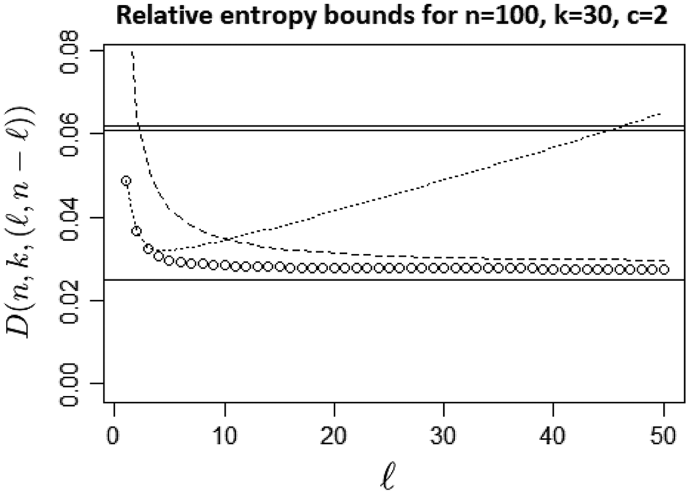


 Open access