1 - Fundamentals of Climate Dynamics

Summary

The chapter describes the basic terminology used in the book, the composition of the Earth system and the principles of climate dynamics. It details the main components of the Earth system (atmosphere, ocean, hydrosphere, cryosphere, biosphere and solid Earth) and processes relevant to understanding climate dynamics. The concepts of climate, climate variability and climate change are discussed in the context of Quaternary climate dynamics. The global cycles of energy, water and carbon and their importance for climate evolution and variability are presented. The chapter introduces the mechanisms behind different types of radiative forcing, climate feedbacks and climate sensitivity. The difference between equilibrium and transient climate responses to different climate forcings is specified. The frameworks of stability and instability are introduced and discussed in application to climate. The relationship between the stochasticity of the Earth system and the predictability of climate change is presented.

1.1 Terminology Related to Stratigraphy

According to the International Chronostratigraphic Table developed by the International Commission on Stratigraphy (ICS), the 4.6 billion years of our planet’s history are divided into eons, eras, periods, epochs and stages, with many dozens of names, mostly derived from Greek words or geographical locations. Importantly, the timing of the beginning and end of all stratigraphic units must be precisely defined and associated with specific geological events. However, these boundaries do not necessarily coincide with major climatic changes or changes in the regime of climate variability.

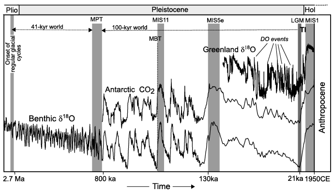
This book is primarily concerned with the Quaternary, which, according to the ISC, began at 2.58 Ma after the end of the Neogene period; 2.58 Ma is also the boundary between the Pliocene and Pleistocene epochs, and this is why it is also known as the Pliocene–Pleistocene Transition (PPT). However, from a climatological point of view, “Quaternary” is primarily associated with the period of time with regular glacial cycles, and the onset of such glacial cycles occurred around 2.7 Ma, that is, significantly earlier than the official PPT. The Quaternary period is divided into two epochs: Pleistocene and Holocene. The latter began at 11.7 ka and thus represents only 0.3% of the Quaternary, while the remaining 99.7% is covered by the Pleistocene. Such a division is difficult to justify from a purely climatological point of view, since the Holocene was, at least until recently, one of more than 50 previous Quaternary interglacial periods. Since the official chronostratigraphic terminology alone is insufficient for describing climate variability during the Quaternary, this book also uses several other terminological systems (see Figure 1.1). One of these is the so-called Marine Isotope Stages (MISs). This name is related to the fact that the MISs are derived from the marine oxygen isotope records. Odd numbers of MISs correspond to interglacial and even numbers to glacial conditions. The exception is the last glacial cycle, which is divided into five MISs, with the additional division of MIS 5 into five sub-substages, of which only MIS 5e is the true interglacial. The Quaternary is divided into more than 100 MISs, while before 2.58 Ma, a different naming system is used to identify climate variability. The names of stages from the International Chronostratigraphic Chart are not used in this book.

Figure 1.1 Selected Quaternary chronological terminology used in this book illustrated by the three most influential paleoclimate records: benthic $\text{δ}{}^{18}\text{O}$, Antarctic and Greenland ice cores. Abbreviations: Plio – Pliocene, the epoch preceding the Quaternary period; Holo – Holocene, officially the current geological epoch, also the name of the current interglacial, equivalent to MIS 1; TI – the last glacial termination or Termination I; LGM – Last Glacial Maximum, time slab corresponding to the time interval 22–19 ka; MIS 5e – previous interglacial, also known as the Eemian interglacial; MIS 11 – the longest interglacial of the late Quaternary and the first interglacial after the Mid-Brunhes Transition; MPT - Mid-Pleistocene Transition, the transition from the 41-kyr to the 100-kyr world.

There are a number of other useful terms used in paleoclimatology to designate different, more or less well-defined time intervals, such as the Last Glacial Maximum (LGM, the interval between 22 and 19 ka), glacial terminations (numbered backwards in time with the most recent Termination I starting at ca. 18 ka and ending at ca. 7 ka) and the Eemian Interglacial (the name of the penultimate interglacial or MIS 5e, between about 130 and 120 ka). Some time intervals, usually associated with significant deviations in paleoclimate characteristics, are called “events” (such as numerous Dansgaard–Oeschger and Heinrich events), and some are called “transitions” (e.g., the mid-Pleistocene Transition – MPT). In this book, all these terms and many others are used for convenience, but usually without any attempt to give strict definitions or their precise timing.

According to the ICS, we are still living in the Holocene epoch, the most recent part of the Quaternary. However, many scientists argue that current human activity has caused significant changes to the environmental conditions in general and the climate in particular, and that there is a need to introduce a new epoch – the Anthropocene. At the time of writing, this idea has been rejected by the ICS Subcommission on Quaternary Stratigraphy, which, of course, cannot prevent the use of the term “Anthropocene” in the scientific literature. Climate change during the Anthropocene is discussed in Chapter 8 of this book.

When time is expressed numerically, it is usually defined as the time before present (BP), but the “present” moves in time. This is not a problem when discussing rather ancient times (millions or thousands of years ago), but for more recent times, it is necessary to define the meaning of “present” more precisely. One possible solution is to use B2K (i.e., before 2000 CE [Common Era]) instead of the present. For the Holocene, especially when applied to the history of human civilization, it is common to use the terms Common Era and Before Common Era. For the future, which will be discussed in the Anthropocene chapter, the use of a Common Era would be appropriate for the current millennium, but for a longer (deep) future, to avoid possible confusion, the year after present (AP) will be used.

It is important to note that, for historical reasons, the opposite direction of the time axis to that commonly used in other branches of science (time increases to the right) is still used in many paleoclimate publications. This book uses exclusively the “physical” direction of the time axis. The standard abbreviations for time are kyr (1000 years), ka (1000 years BP) and Ma (million years BP), where BP is before present (in case the accuracy of the time definition is significantly less than 100 years) and B2K is before the year 2000 CE, for a more accurate time scale. Note that in paleoclimatology, the term “age model” is often used as a synonym for time.

1.2 Earth System

1.2.1 Earth as the Planet

The Earth is the third planet in the Solar System and the only known habitable planet in the Universe. The Earth’s climate is largely controlled by astronomical parameters such as the luminosity (total amount of energy emitted into space in a unit of time) of the nearest star (the Sun) around which the Earth orbits, the distance to that star, the radius and mass of the Earth, the period of its rotation on its axis and the angle between the plane of rotation around the Sun and the Earth’s axis of rotation. Some of these characteristics change over time and cause climate change. The solar luminosity gradually increasing due to the typical life cycle of Sun-like stars (gradual internal heating and expansion). It is thought that 4000 Ma ago, the solar luminosity was about 25% lower than today. However, during the Quaternary, the long-term trend in solar luminosity has been negligible. Solar luminosity also varies on much shorter time scales (periods of 11, 80 and 200 years), but these variations are very small (on the order of 0.1% of the average solar “constant”) and likely of little importance for understanding past climate change.

The Earth orbits the Sun along an ellipse that is currently very close to a circle. The parameters of the Earth’s orbit (eccentricity and the so-called precession parameter) and the angle between the direction of the Earth’s axis of rotation and the plane of its rotation around the Sun (obliquity) vary in time with several periods ranging between 20,000 and 2 million years. These variations in the Earth’s orbital parameters play a crucial role in Quaternary climate variability (see Box 1.1).

By far the largest source of energy affecting climate and life is the Sun. This is more than three orders of magnitude larger than the geothermal heat flux, but the latter still plays an important role in ice sheet dynamics and affects deep ocean temperature. The dissipation of tidal energy associated with the gravitational interaction with the Moon and Sun is an order of magnitude smaller, but is important for vertical mixing in the deep ocean and thus for global ocean circulation and energy transport. A large amount of energy is currently produced by human activity, mainly through the burning of fossil fuels. Note that this does not include the greenhouse effect of the greenhouse gases produced, which is several orders of magnitude greater than the direct heat produced by combustion. So far, this heat emission has only a local direct effect on climate.

The rate at which the Earth rotates on its axis determines the length of day and night and strongly influences atmospheric and oceanic dynamics through the so-called Coriolis force. The angular rate of the Earth’s rotation has been decreasing since the formation of the Earth due to tidal dissipation, but over the last few million years, it can be considered constant.

The presence of an ocean and the composition of the atmosphere are two closely related factors that strongly influence climate and are critical for the existence of life, which in turn influences the composition of the atmosphere. They are the result of a very long-term co-evolution of different components of the Earth system.

1.2.2 Atmosphere

The term “climate” has historically referred to the average state of the atmosphere, although it is now used in a broader sense to include other components of the Earth system, such as the hydrosphere and cryosphere. Nevertheless, in the discussions of climate and climate change, atmospheric properties such as near-surface air temperature and precipitation are given primary attention.

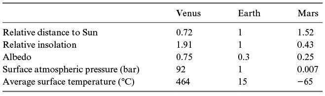
The Earth’s atmospheric composition and mass are radically different from those of two neighboring Earth-type planets – Venus and Mars (see Table 1.1). This is explained by the presence of water and life on Earth. While the atmospheres of Venus and Mars consist mainly of CO₂, the Earth’s atmosphere consists mainly of nitrogen and oxygen. The current CO₂ concentration in the Earth’s atmosphere is about 0.04%, while the preindustrial concentration was 0.028%.

Table 1.1Comparison of the key Earth parameters with Mars and Venus

	Venus	Earth	Mars
Relative distance to Sun	0.72	1	1.52
Relative insolation	1.91	1	0.43
Albedo	0.75	0.3	0.25
Surface atmospheric pressure (bar)	92	1	0.007
Average surface temperature (°C)	464	15	−65

Note: Venus and Martian atmospheres consist mostly of CO₂, while the CO₂ concentration in the Earth’s atmosphere is currently 0.04%. The difference in insolation between Earth and Mars can only explain about 40°C difference, while in reality, it is almost twice as large. The reason is that the greenhouse effect makes the Earth about 33°C warmer than it would be without the greenhouse effect, while the Martian atmosphere is too thin to cause a significant greenhouse effect. Venus, with its high albedo, should be even colder than the Earth without the greenhouse effect. In fact, it is 450°C warmer than Earth because of a much stronger greenhouse effect.

The composition of the atmosphere is one of the key factors determining the Earth’s climate and has changed drastically over the past 4 billion years due to geochemical and biological processes. Most constituents of the atmosphere are well mixed – that is, have nearly constant concentrations in space and time (at least on an annual time scale), except in the upper atmosphere. Two gases dominate the Earth’s atmosphere – nitrogen and oxygen (together 99%) – but their concentrations remain nearly constant on time scales of millions of years and so do not play an active role in Quaternary climate change. There are three other well-mixed gases that make up a much smaller fraction of atmospheric mass, but because they are greenhouse gases (i.e., they actively absorb infrared radiation), they play a significant role in past climate changes, particularly during the Quaternary: carbon dioxide (CO₂), methane (CH₄) and nitrous oxide (N₂O). Concentrations of these gases varied almost synchronously with Quaternary glacial cycles and played a key role in past climate change. These three gases, especially CO₂, are also the main drivers of current anthropogenic global warming.

There are a few important gases that have a relatively short lifetime in the atmosphere, so their concentrations vary considerably over time and space. These are water vapor and ozone. Since most of the Earth’s surface is covered by the ocean, the atmosphere contains a significant amount of water vapor (up to 1% near the ocean surface in the tropics), but the concentration of water vapor decreases rapidly with altitude and toward the poles. Water vapor is the main greenhouse gas in the Earth’s atmosphere and explains most of the natural 33°C greenhouse effect. It also plays a major role in horizontal energy transport in the atmosphere and forms clouds, which play an important role in the Earth’s radiative budget and hydrological cycle.

The lifetime of ozone is controlled by chemical reactions. Stratospheric ozone is formed by photochemical reactions, and its concentration decreases from the equator to the poles. Ozone is important for the Earth’s radiation budget because it absorbs most of the UV radiation. For the same reason, it is important for human health, which is why the depletion of ozone over Antarctica observed in recent decades (the “ozone hole”) has caused serious concern in the past.

In addition to gases, the Earth’s atmosphere always contains a certain amount of impurities such as dust and salt particles, black carbon and sulfur aerosol. Although in relatively small concentrations, different types of aerosol play important roles in climate and climate change through their direct influence on the Earth’s radiative balance and indirect influence through cloud formation. Aerosol deposition over snow cover can also affect its albedo, and in the ocean, dust deposition also affects the ocean carbon cycle.

The most important climatological property of the atmosphere is its temperature. The three-dimensional temperature field in the atmosphere is influenced by, and in turn controls, atmospheric radiative processes, atmospheric circulation and the hydrological cycle. In particular, atmospheric temperature is affected by absorption and emission of radiation (both shortwave and infrared), phase transitions (condensation), vertical mixing, advection by large-scale and mesoscale motions, and other processes. Therefore, accurate modeling of the atmospheric temperature distribution, and consequently of other atmospheric properties, is a serious challenge. In addition, atmospheric temperature and the associated energy exchange strongly influence the ocean, cryosphere and biosphere.

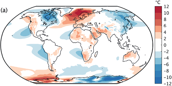
The temperature in the troposphere (the lowest 10–15 km), averaged over the climatological time scale, decreases approximately linearly with altitude, and the average lapse rate (vertical temperature gradient) in the troposphere is close to 6°C/km. The horizontal temperature distribution is mainly controlled by the insolation (which depends on latitude and season), the planetary albedo and the horizontal energy transport in both the atmosphere and the ocean. The seasonal distribution of insolation is controlled by the Earth’s astronomical parameters, which vary with orbital periods of 10⁴–10⁵ years. These variations are the direct cause of the Quaternary glacial cycles and associated climate variability. The areas where the ocean releases large amounts of energy to the atmosphere are also characterized by positive temperature anomalies relative to the zonally averaged annual mean temperatures (see Figure 1.2a). This explains numerous and significant regional temperature changes observed on millennial time scales during most of the Quaternary. In addition, seasonal temperature variations strongly depend on the heat capacity of the underlying surface and are much larger in the continental interior than in the ocean (see Figure 1.2b).

Figure 1.2

(a) Deviation of the annual mean surface air temperature, corrected for the elevation effect, from the zonal mean temperatures

Figure 1.2a long description..

Figure 1.2(a)Long description

Global deviations in annual mean surface air temperature after correcting for elevation effects. The scale ranges from negative 12 degrees Celsius to positive 12 degrees Celsius. Strong warm anomalies appear near the Arctic, Northern Europe, Western Antarctica, and some parts of North America. Cooler anomalies appear around Eastern Antarctica, the Oceans, and Eastern Russia.

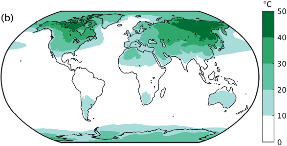
(b) The magnitude of the seasonal variations of the surface air temperature computed from ERA-Interim reanalysis data.

Figure 1.2b long description..

(Dee et al. 2011)

Figure 1.2(b)Long description

Global magnitude of the seasonal variations of the surface air temperature. The scale ranges from 0 degrees Celsius to 50 degrees Celsius. The highest seasonal variation ranges appear near North America, Europe, and Northern Asia. Moderate seasonal variation ranges appear near South America and Southern Africa. Lesser seasonal variation ranges appear near Australia and the oceans.

The distribution of water vapor (expressed in terms of specific humidity) in the atmosphere is closely related to air temperature, since the specific humidity of saturated water vapor is an exponential function of air temperature. Therefore, to a first approximation, the vertical profile of specific humidity can be approximated by the exponent with a vertical height scale of about 2 km. The distribution of relative humidity is mainly controlled by the atmospheric circulation and the type of underlying surface (ocean or land). As the most important greenhouse gas, water vapor is responsible for the strongest positive climate feedback, amplifying climate changes caused by other greenhouse gases and other climate forcings. Water vapor transport is an essential element of the global hydrological cycle, strongly influencing ocean circulation, the cryosphere and the biosphere. Condensation of water vapor leads to cloud formation, which plays an equally important role in controlling climate and climate change. The set of cloud-related climate feedbacks represents the main uncertainty in modeling the climate response to changes in atmospheric CO₂ concentration. The amount of water which condensates in the atmosphere and then precipitates, together with air temperature, determines the spatial distribution of vegetation.

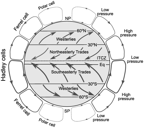
Atmospheric circulation (i.e., the movement of air, usually referred to as wind) is a complex three-dimensional phenomenon with a wide range of temporal and spatial scales (see Figure 1.3). It plays a fundamental role in climate and climate change. The global circulation of the atmosphere includes such large-scale (>10³ km) phenomena as the trade winds, westerlies, monsoons and the meridional cells of the atmospheric circulation. The latter are represented by three pairs of cells: Hadley, Ferrel and Polar cells. This complex circulation results from the interplay between temperature gradients from the equator to the poles and the rotation of the Earth around its axis. This qualitative circulation pattern is robust to a wide range of global climates, but seasonal variations in the intensity and meridional extent of individual cells are influenced by climate and, in turn, affect climate. For example, asymmetric temperature changes in different hemispheres lead to a meridional shift in the position of two Hadley cells, affecting the location of the Intertropical Convergence Zone (ITCZ). At the same time, global warming or cooling causes the Hadley cells to expand or contract. This zonally averaged meridional circulation is a major contributor to the sea level pressure patterns that drive the major zonal winds known as the trades and westerlies. Again, this pattern is fairly stable across different climates, but the strength and position of both wind systems are affected by climate change. Another element of atmospheric circulation that strongly influences regional climate and is sensitive to climate change is the monsoon circulation. There is both empirical and modeling evidence that the strength of the south-east Asian monsoon, for example, has varied greatly both during glacial cycles and during millennial climate changes.

Figure 1.3 Large-scale atmospheric circulation for northern summer conditions. The Intertropical Convergence Zone is shifted north of the equator, the southern Hadley cell is stronger and wider than the northern one, and the southern zonal winds are stronger than the northern ones.

Figure 1.3 long description..

Figure 1.3Long description

The diagram shows by arrows the direction of the westerlies (winds blowing eastwards) and trades (winds blowing westwards) in both hemispheres for northern summer conditions when the Intertropical Convergence Zone is located north of the equator. The figure also shows the main cells of the atmospheric meridional circulation and the direction of air movement in these cells. The figure also shows the location of low-pressure areas (equatorial belt and high latitudes of both hemispheres) and high-pressure areas (subtropics).

1.2.3 Hydrosphere

The Earth is unique in having a large amount of water in liquid form on its surface, known as the hydrosphere. Most of the water is found in the oceans, which play a fundamental role in the climate system as an essentially unlimited source of water for the energy and water cycles. According to geological data, the ocean has been present for most of the Earth’s 4 billion years of history. The presence of the ocean is thought to be crucial to both the existence of life and plate tectonics.

The world’s oceans contain about 97% of the Earth’s water and cover 71% of the Earth’s surface. During the late Quaternary glacial cycles, the volume of the ocean varied by 3% and its area by about 6%. Unlike the atmosphere, which is global, the ocean consists of three major ocean basins separated by continents and connected mainly by the circumpolar Southern Ocean. Plate tectonics changes the geographical patterns of the oceans on geological time scales, but during the Quaternary the configuration of the ocean (apart from shelf areas affected by sea level changes) was very similar to that of today.

The modern ocean has an average depth of 4000 km, and its heat capacity per unit area exceeds that of the atmosphere by three orders of magnitude. The ocean is therefore an important heat reservoir on time scales from seasonal to centennial. Even considering only the upper layer of the ocean, the heat capacity of the ocean is one to two orders of magnitude greater than that of the atmosphere. As a result, the ocean absorbs a large amount of energy in summer and releases it in winter, significantly reducing the amplitude of seasonal temperature variations. The difference between maximum and minimum temperatures over open water does not usually exceed 10°C. The heat released by the ocean is transported by the atmosphere to the surrounding land, where the air cools rapidly in winter, so that the moderating effect of the ocean diminishes toward the continental interior (see Figure 1.2b).

Unlike the atmosphere, most of the ocean is stably stratified, mainly due to a decrease in temperature with depth. As a result, vertical mixing is efficient only in the upper mixed layer, typically a few tens to a few hundred meters deep, below which vertical mixing is very weak. Only in a few rather small areas in the high latitudes of the Atlantic and near Antarctica could surface cooling during winter destabilize a significant part of the water column. Although these areas are small compared to the ocean as a whole, they play a very important role in ocean circulation and therefore in climate. Because the deep ocean is filled with water masses formed at high latitudes, the global volume-averaged temperature of the ocean is only 4°C, while the average sea surface temperature is 18°C.

Ocean water contains about 3.5% salt per unit mass. Although the total salt content of the ocean changes only on geological time scales, local salinity, defined as the amount of salt per kilogram of seawater, changes significantly, especially in the upper ocean. The presence of salt in the water plays an important role in the ocean. At low temperatures, the effect of salinity on seawater density is comparable to that of temperature. Because salinity affects vertical mixing and ocean circulation, the large-scale ocean circulation is still often called “thermohaline circulation,” that is, driven by temperature and salinity (the Latin word “haline” means salt). The presence of salt in seawater also eliminates an anomalous property of freshwater related to maximum density. Freshwater reaches its maximum density at about 4°C. Further cooling makes the water lighter. This makes it easier for ice to form in freshwater. In the sea, the maximum density is not reached before the freezing point at −1.8°C for average ocean salinity.

The oceans transport energy from the tropics to the high latitudes that is comparable to the amount of energy transported by the atmosphere (see Section 1.3). The energy is transported by several types of processes: meridional overturning circulation, Ekman transport, ocean gyre circulation and transient synoptic eddies. The Atlantic Meridional Overturning Circulation (AMOC), has attracted particular attention, as both empirical data and modeling results suggest that this type of circulation experienced significant and sometimes very abrupt variations during the Quaternary, causing large climate changes at both regional and global scales. This variability of the AMOC is attributed to its intrinsic instability under cold glacial climatic conditions (see Chapter 6). However, although it may seem counterintuitive, model simulations suggest that a significant weakening of the AMOC may also occur in the relatively near future in response to anthropogenic climate warming (see Chapter 8). Currently, the AMOC transports more than 1 PW of energy northwards across the equator. This energy is released over relatively small areas of the ocean, and there are regions, such as the North Atlantic, where the annual mean energy flux from the ocean to the atmosphere reaches 100 W/m², a value comparable to the energy received from the Sun. Therefore, a complete shutdown of the AMOC leads to a decrease in the annual mean surface temperature of about 10°C in the areas where heat is currently being released into the atmosphere. The pattern of climate response to AMOC shutdown is similar to that of present-day azonal temperature anomalies (Figure 1.2a).

Other elements of the hydrosphere, such as lakes, rivers and groundwater, also play an important role in the hydrological cycle, although they contain much less water. In particular, rivers redistribute water over long distances and provide significant freshwater input to the ocean, affecting ocean circulation. During glacial periods, some rivers routing changed significantly compared to modern times due to blockage by ice sheets and changes in topography. This, in turn, can lead to a significant change in the area of the ocean that receives meltwater from the ice sheet. Lakes are an important source of local precipitation and can act as important positive feedback, explaining, for example, the “green Sahara” phenomenon during the mid-Holocene and earlier interglacials. During glacial periods, proglacial lakes formed during ice sheet retreat can, in turn, significantly affect ice sheet mass loss and hence the rate of retreat (see Chapter 5).

1.2.4 Cryosphere

The cryosphere is defined as all water in solid form, that is, snow, sea ice, permafrost (i.e., frozen ground water), glaciers and ice sheets. Snow cover (both land, sea ice and ice sheets) plays an important role in surface and planetary albedo and contributes significantly to the albedo-climate feedback. Sea ice also contributes to albedo, but it also affects ocean circulation and the exchange of energy, water and gases between the ocean and the atmosphere. Permafrost stores a significant amount of carbon, which can be released into the atmosphere when the permafrost thaws. However, ice sheets play by far the most important role in Quaternary climate dynamics. Ice sheets are the slowest component of the climate system. A typical response time of ice sheets to orbital or radiative forcing is on the order of thousands to tens of thousands of years, that is, comparable to the time scales of orbital forcing. Ice sheets are therefore never in equilibrium and their response to external and internal forcings is fundamentally transient.

Two existing at present ice sheets – Antarctic and Greenland – contain the amount of ice that, if melted completely, would raise global sea level by about 65 meters. During the Quaternary, two other major ice sheets were periodically formed over North America and Eurasia, and the global volume of ice sheets during the Last Glacial Maximum was about three times greater than today, with ice sheets covering up to 10% of the Earth’s surface. Understanding the processes by which ice sheets translate regional and seasonal changes in insolation caused by variations in Earth’s orbital parameters to global scale long-term climate change is one of the major challenges of Quaternary climate dynamics and is discussed in Chapter 6.

The temporal evolution of ice sheets is primarily controlled by their mass balance and internal dynamics. For land-based ice sheets, the mass balance is essentially a surface mass balance is determined by accumulation (mainly snowfall) and surface melt, most of which occurs at low elevations. Where ice sheets extend into the ocean, calving (iceberg formation) and melting at the base of ice shelves or glaciers in the ocean can also play an important role in the mass balance of the ice sheet. The accumulation of ice in the center of ice sheets and the melting or calving at the margins creates a gradient in ice sheet surface elevation, which drives the dynamics of the ice sheets. To a first approximation, ice can be considered as a very viscous but non-Newtonian fluid, since ice viscosity depends strongly on temperature and internal stress. Typical velocities in the interior of the ice sheet are on the order of several meters to 100 meters per year. At the margins, and especially in ice streams, the ice can move much faster, up to several kilometers per year. The rate of movement of the ice sheet depends on the thickness and slope of the ice sheet, and even more so on the state of the base of ice sheet. There are two main types of basal conditions – one is when the temperature at the base of the ice is below the pressure melting point (which is 0°C at zero pressure and decreases by about 1°C for every kilometer of ice thickness). If the ice is frozen to the bed, the horizontal velocity of the ice at the base is close to zero. However, if the base of the ice sheet is at the pressure melting point and there is a (usually very thin) layer of water separating the ice from the bedrock, the ice can slide and move much faster.

The Antarctic and Greenland ice sheets have existed for millions of years, but new ice sheets can form relatively quickly in the high latitudes of the NH under favorable climatic conditions, such as cold summers during periods of low summer insolation. The formation of a new ice sheet requires an area of perennial snow cover, which can continuously accumulate snow and form an ice cap. Initial ice caps can then expand laterally and grow into a large ice sheet on a time scale of thousands of years. During this growth phase, several positive feedbacks play an important role. First, the increase in the area of the ice sheet, at least initially, proportionally increases the total accumulation of snow. Second, the surface albedo of the ice sheet is significantly higher than that of ice-free land under the same climate conditions. This increases the planetary albedo above the ice sheet, reducing the absorbed solar radiation and leading to strong regional cooling. This in turn reduces surface melting and makes the overall surface mass balance of an ice sheet more positive. The third is the elevation feedback. This is related to the fact that the atmospheric temperature typically decreases by 4–6°C per kilometer of altitude. The downward longwave radiation flux also decreases with altitude. This leads to a reduction in both sensible heat flux and absorbed longwave radiation. As a result, the higher the ice sheet, the less it melts.

Since the Quaternary ice sheets did not grow indefinitely, there must also be some negative feedbacks. One is related to the fact that as the ice sheets expand southwards (in the NH), the ambient atmospheric temperature rises and so does the surface melt. Another negative feedback, known as the desert-elevation feedback, is related to a reduction in precipitation over high and extensive ice sheets. While total precipitation continues to increase with the size of the ice sheet, most of the precipitation occurs over the ice sheet margins, with very little snowfall occurring in the central part of the ice sheet.

The above-mentioned processes and feedbacks are only a part of the large number of feedbacks and processes associated with ice sheet-climate interactions (see Figure 1.4). In particular, ice sheets also modify atmospheric circulation and precipitation patterns. According to model simulations, the growth of the Laurentide ice sheet leads to a strengthening of the westerlies over the Atlantic, which also affects the circulation of the Atlantic Ocean. At the same time, stationary topographic waves associated with high ice sheets affect the temperature in the areas away from the ice sheet. Model simulations show that the changes in atmospheric circulation caused by a large Laurentide ice sheet lead to pronounced warming west of the ice sheet.

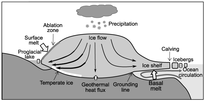
Figure 1.4 Conceptual scheme of the interaction between climate and the ice sheet under glacial climate conditions.

Figure 1.4 long description..

Figure 1.4Long description

The diagram shows a vertical cross-section of a typical land-based ice sheet and associated ice shelf. The arrows within the ice sheet indicate the direction and speed of ice movement. It also shows the location of the ablation zone (the surface of the ice sheet at low altitude) and the location of the temperate ice (ice at the pressure melting point) at the base of the ice sheet. They also show major processes and fluxes, such as geothermal heat flux at the base of the ice sheet, calving of icebergs into the ocean and proglacial lakes, and basal ice melting in the ocean.

Another important ice-sheet-climate interaction is related to the melting of the ice sheet and the calving of icebergs, which produce large amounts of freshwater. The average net freshwater flux from the ice sheets to the oceans (mainly the North Atlantic) during past glacial cycle was 0.1 Sv, but it can be significantly larger during certain intervals, such as Heinrich events. A large meltwater flux during glacial termination may be sufficient to significantly weaken the AMOC, reducing warming, over the North Atlantic and western Europe, which reduces surface melting of the ice sheets, and thus provides a significant negative feedback. Beyond these regional processes, changes in the ice sheets cause global sea level rise and fall. This affects climate, dust and carbon cycles around the globe.

1.2.5 Biosphere

The biosphere is the zone of air, water and land where life exists. While it includes most of the troposphere and the entire ocean, on land it is concentrated in a relatively thin layer of soil and just above the land surface. The total mass of the biosphere is rather small compared to other elements of the Earth system, but it plays an important role in past climate variability by controlling atmospheric composition, weathering rate, surface albedo and roughness, and the global hydrological cycle. The most important consequence of the existence of life on Earth is the high concentration of oxygen and low concentration of CO₂ in the Earth’s atmosphere. Until recently, the biosphere was also the main source of methane.

The natural terrestrial biosphere (vegetation cover) is largely controlled by climate characteristics, such as summer and winter temperatures and annual precipitation. This fact has already been used in the Köppen climate classification. However, a one-to-one correspondence between climate and vegetation distribution can only be expected under constant climatic conditions, and in the case of climate change, vegetation dynamics must be taken into account. The time scales of the equilibration between climate and vegetation cover are not well known, but it is clear that the time scales can be very long (hundreds of years to millennia). In addition, more than 50% of the land surface is currently influenced by humans in one way or another.

The terrestrial biosphere, primarily vegetation, is not only controlled by the climate but also influences it in a number of ways. In particular, the presence of vegetation affects the albedo of the land surface. Land covered by dense vegetation has a lower albedo than bare soil, and even when vegetation is sparse, the presence of organic carbon in the soil makes it much darker than that of a sandy desert such as the Sahara. However, the difference in albedo between snow-covered forest and non-forest (grassland or bare soil) is particularly significant. While the surface albedo of the snow layer over a flat surface can be as high as 0.8, a forest, even when covered by snow, remains relatively dark with a typical albedo of 0.2–0.3. Summer warming in the boreal latitudes causes the forest to expand northwards, lowering the albedo and causing additional warming, creating a positive climate-vegetation feedback, also known as the taiga–tundra feedback (see Section 1.6). Vegetation also affects the global water cycle through evapotranspiration. Transpiration depends on climate, but also directly on CO₂ concentration through stomatal resistance. In practice, this means that under the same climatic conditions, vegetation will evaporate less water at high CO₂ levels, leading to additional regional warming. In addition to living biomass, much of the organic carbon on land is stored in peat and permafrost. These carbon pools have large capacity and long residence times and contribute to glacial-interglacial CO₂ variations. During the late Holocene, deforestation caused significant CO₂ emissions to the atmosphere and contributed to the observed anthropogenic climate change. The terrestrial biosphere is known to have been a significant net sink of anthropogenic CO₂ (about 25% of anthropogenic emissions). In the future, however, thawing permafrost and soil degradation could become significant long-term sources of CO₂. The presence of large amounts of organic carbon in soils affects weathering rates and thus atmospheric CO₂ concentrations on the geological time scales. The terrestrial biosphere (mainly wetlands and termites) plays an important role in the methane cycle.

The marine biosphere is one of the smallest carbon pools. However, the carbon fluxes associated with the marine biosphere are not small, which is explained by the very fast turnover time of the marine biosphere. Most of the living marine biomass is concentrated in a thin (on the order of a hundred meters) upper layer of the ocean, where the intensity of sunlight is still sufficient for photosynthesis. Sinking organic matter and biologically produced calcites (shells) provide an important carbon flux to the deep ocean (biological pump). Changes in biological production as well as temperature-dependent remineralization rates, are the factors that influence the strength of the biological pump and thus the storage of carbon in the deep ocean, which is thought to be an important factor in explaining glacial-interglacial variations in CO₂.

1.2.6 Solid Earth

Solid Earth processes beyond the top few meters of soil are not usually considered when studying short-term climate change. However, on longer time scales, the solid Earth is an important element in climate dynamics. First, plate tectonics, through changes in the position and elevation of the continents and the bathymetry of the oceans, affects the radiative balance of the climate system, atmospheric and oceanic circulation, and the global water and carbon cycles. In particular, the formation of high mountain ridges such as the Himalayas and the Tibetan Plateau has strongly influenced atmospheric circulation, in particular by enhancing monsoon circulation and summer precipitation.

Second, plate tectonics controls the release of CO₂ through volcanoes and deep-sea hydrothermal vents. This has a direct effect on the atmospheric CO₂ concentration because, on long time scales, atmospheric CO₂ is controlled by the balance between volcanic outgassing and chemical weathering rates. The rate of uplift can also affect weathering, since the weathering rate of newly exposed rocks is much higher than that of old rocks and terrestrial sediments. It has been proposed that the last phase of the Cenozoic cooling was largely caused by increased weathering due to unusually rapid continental uplift. In addition to the permanent volcanic CO₂ outgassing, the most powerful volcanic eruptions can affect the climate regionally and globally on time scales of several years, mainly through the formation of the sulfur aerosol layer in the stratosphere, which increases the reflection of sunlight.

On time scales of less than a million years, the position of the continents and surface orography can be considered constant, with the notable exception of areas periodically covered by large ice sheets. Ice loading lowers the lithosphere by about 1/3 of the thickness of the ice sheet, typically about 1 km. This lithospheric adjustment plays an important role in ice sheet dynamics, especially during glacial terminations. The typical relaxation time scale of lithospheric rebound depends on mantle viscosity and is in the range of 1000–10,000 years. Therefore, relatively rapid retreat of ice sheets during glacial terminations leads to the formation of periglacial lakes and inundation of continents by the ocean.

Another process related to the interaction between ice sheets and the solid Earth is glacial erosion. Advancing ice sheets transport terrestrial sediments toward the ice sheet margins. As a result of repeated glacial advances, the northern parts of North America and Scandinavia are largely devoid of terrestrial sediments, consisting primarily of exposed bedrock covered by only thin layers of soil. This process is considered crucial in explaining changes in the dominant periodicity of glacial cycles about 1 million years ago.

After the terrestrial sediments were removed, the waxing and waning of the ice sheets began to erode the bedrock, creating fjords, straits and inlets. The present Arctic Archipelago has been shaped by numerous advances of the North American Ice Sheet and was a relatively flat part of the North American continent prior to the Quaternary. Hudson Bay and the Hudson Strait are thought to have been formed by glacial erosion less than 1 million years ago. The presence of deep fjords and straits influences the dynamics of the ice sheet through the development of fast ice streams.

Finally, the geothermal heat flux, although rather small (in most cases less than 0.1 W/m² on continental plates), plays an important role in ice sheet dynamics. Without this flux, ice sheets would be much less mobile, as they would have smaller areas of temperate ice at the base where rapid sliding is possible.

1.3 Global Energy, Water and Other Material Cycles

1.3.1 Earth Energy Budget

The amount of solar energy received by the Earth is determined by the so-called “solar constant,” which in reality is not exactly constant and is defined as the solar radiation per unit area perpendicular to the direction of the Sun’s rays at the average distance from the Sun to the Earth. This value is currently close to 1361 W/m². This value has changed significantly over geological time scales, increasing by about 10% over the last billion years. The average amount of radiation absorbed per unit area of the Earth’s surface is about 240 W/m², giving a total of about 125 PW (see Figure 1.5). This total depends on the planetary albedo, which in turn is mainly controlled by surface albedo and cloud cover. During glacial periods, the surface albedo changed significantly over areas covered by ice sheets, reducing the amount of radiation absorbed globally by up to 3 W/m², or about 1%.

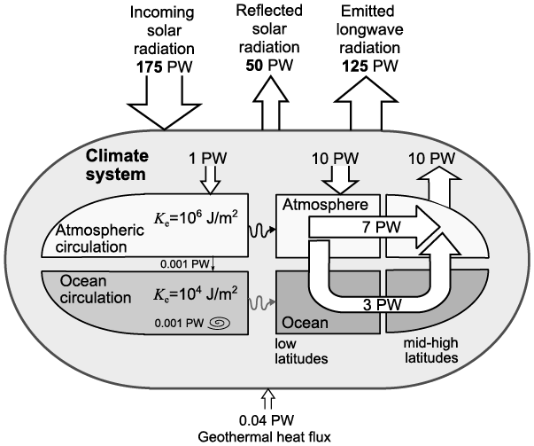
Figure 1.5 Global-scale energy balance and transport in the climate system. The climate system receives about 175 PW (1 PW = 10¹⁵W) of energy from the sun, of which 50 PW is reflected and 125 PW is emitted into space as longwave (infrared) radiation. Only about 1 PW of the absorbed energy is converted into kinetic energy in the atmosphere, and even less (about 0.001 PW) is transferred to ocean motion. A further 0.001 PW comes from the dissipation of tidal energy.

Figure 1.5 long description..

Figure 1.5Long description

The diagram shows the whole Earth system as an oval. Large arrows at the top of the oval indicate global incoming solar energy (175 petawatts), reflected solar energy (50 petawatts), and outgoing longwave radiation (125 petawatts). The total geothermal flux of 0.04 petawatts is shown at the bottom of the oval. Inside the oval, four segments illustrate the redistribution of energy within the atmosphere and ocean. The left segments show the transformation of the total energy flux into kinetic energy of atmospheric motion (1 petawatt) and kinetic energy of ocean circulation (0.001 petawatt). The right segments show that 7 petawatts of energy is transported in the atmosphere from low to high latitudes, while the ocean transports 3 petawatts.

On time scales much longer than a year, the radiative balance of the Earth system is close to zero, that is, the amounts of radiation absorbed by Earth and emitted back into space are very close to each other. The peculiarity of the Earth’s atmosphere is that it is sufficiently transparent to shortwave solar radiation, of which more than 50% reaches the Earth’s surface, but due to the presence of water vapor, CO₂ and other greenhouse gases, the atmosphere is opaque to outgoing infrared radiation, and only 5% of the energy emitted from the Earth’s surface escapes directly into space through a narrow window in the absorption spectra of the atmosphere. The rest is absorbed in the atmosphere and re-emitted both upwards and downwards. Thus, a significant fraction of the absorbed solar energy is “recycled” many times within the atmosphere before it is able to leave it. This is the essence of the natural greenhouse effect, which for the preindustrial atmosphere was about 32°C in terms of global annual surface air temperature. This means that if the Earth’s atmosphere did not contain greenhouse gases, the surface temperature would be –18°C instead of the observed 14°C. During glacial times, reduction in CO₂ concentration (and to a lesser extent methane and N₂O) directly and through positive climate feedbacks reduced the natural greenhouse effect by about 3°C, which is comparable to the direct effect of ice sheets on surface temperature. At present, an anthropogenic increase in atmospheric concentrations of greenhouse gases (in this case water vapor acting as a positive feedback) has led to an additional 1.5°C of global warming compared to preindustrial times.

Water plays a fundamental role in the Earth’s energy budget, not only as the main atmospheric greenhouse gas, but also through phase transitions and the associated latent heat transfer. The heat flux from the Earth’s surface to the atmosphere through evaporation is equal to almost half of the absorbed solar radiation. The horizontal transport of moisture in the atmosphere also accounts for a significant fraction of the meridional energy transport in the Earth system.

Only a small fraction of the solar energy absorbed by the Earth (less than 1%) is converted into kinetic energy in the atmosphere, and three orders of magnitude less is converted into kinetic energy of the ocean circulation. The Earth system is therefore an extremely inefficient heat engine. Nevertheless, the oceanic and atmospheric circulations redistribute significant amounts of energy between low and high latitudes: about 10 PW, or more than 10%, of the amount of solar energy absorbed at low latitudes (between 30°S and 30°N) is transferred by the atmosphere and ocean to the extratropics, making the Earth’s climate much more equable (see Figure 1.5). The atmosphere transfers more energy than the ocean, mainly through the meridional atmospheric circulation in the tropics and through the synoptic eddies (cyclones and anticyclones) at high latitudes. In the ocean, heat transport is dominated by the meridional overturning circulation (in the Atlantic) and by horizontal gyres and synoptic eddies elsewhere. While ocean eddies play a rather small role in meridional ocean heat transport, they contain most of the oceanic kinetic energy and play an important role in ocean dynamics.

1.3.2 Global Water Cycle

The global hydrological cycle plays an important role in the climate system and climate change for a number of reasons. First, evaporation, condensation and horizontal moisture transport in the atmosphere are important components of the Earth’s energy balance and energy transport. Second, water vapor is the most important greenhouse gas and provides a strong positive feedback for climate change caused by other factors. Third, clouds play a critical role in the energy balance of the climate system. Fourth, the balance between evaporation and precipitation affects the salinity of the ocean surface and hence the ocean circulation. Fifth, the hydrological cycle largely determines the evolution of ice sheets. Finally, precipitation determines spatial patterns of vegetation cover, especially in the subtropics.

In contrast to energy, atmospheric moisture in the tropics is transported toward the equator, and only outside the tropics is it transported toward the poles. This is related to the meridional atmospheric circulation – the Hadley and Ferrell cells. Latitudinal zones characterized by ascending air have high precipitation, and zones with descending air have low precipitation. As a result, the zonal distribution of precipitation is characterized by a strong maximum at the equator and smaller maxima in the midlatitudes, with local minima in the subtropics. Meridional moisture transport at high latitudes is dominated by synoptic eddies. As the water holding capacity of air is lower at low temperatures, precipitation has a tendency to decrease toward the poles.

Due to the strong dependence of water vapor on temperature, the hydrological cycle is significantly enhanced with global warming and weakened with cooling, but this does not mean that precipitation increases/decreases everywhere with higher/lower temperatures. This is due to the strong influence of atmospheric dynamics on precipitation. As the position and width of the Hadley cell depend on the climate state, this factor explains the complexity of the response of precipitation to climate change. At regional and local scales, the Earth’s topography strongly influences the distribution of precipitation. On geological time scales, mountain uplift leads to a large spatial redistribution of precipitation. On astronomical time scales, the retreat and growth of ice sheets cause pronounced changes in atmospheric dynamics and precipitation. Another component of atmospheric dynamics that strongly influences regional precipitation patterns is the monsoon circulation. Both paleoclimate records and model simulations show that the monsoon circulation is highly sensitive to changes in Earth’s orbital parameters and reorganizations of the AMOC.

More than half of the water that precipitates over land then evaporates back into the atmosphere, and the rest is returned to the oceans through river and groundwater flows. Because the flow of water to the ocean is controlled by surface elevation, changes in river routing are very slow. However, the growth of large continental ice sheets during glacial periods can block some rivers, form periglacial lakes and significantly alter surface water fluxes. In addition, ice sheets themselves are important sources of freshwater for the ocean, both in the form of surface runoff and the solid ice discharge (icebergs calving), which can melt far from where they are formed.

1.3.3 Global Carbon Cycle

Since CO₂ is the main well-mixed greenhouse gas responsible for a significant fraction of climate variability throughout Earth’s history, understanding the carbon cycle is very important for climate dynamics. Although the atmosphere is a very small reservoir of carbon compared to the ocean and the Earth’s crust, the amount of carbon in the atmosphere to a large degree determines climate. The atmosphere interacts with other carbon reservoirs in a rather complicated way (see Figure 1.6), and this interaction gives rise to several positive and negative climate-carbon cycle feedbacks.

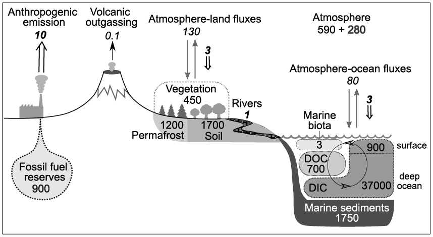
Figure 1.6 Global carbon cycle. Regular numbers indicate the size of carbon pools in GtC (10⁹ tonnes in carbon equivalent), italic numbers correspond to annual carbon fluxes in GtC/yr. Bold italic numbers correspond to anthropogenic CO₂ emissions and fluxes associated with anthropogenic activities (both fossil fuel combustion and land use). Bold regular number indicates change in the atmospheric inventory due to anthropogenic emissions. DOC stands for the dissolved organic carbon and DIC for the dissolved inorganic carbon.

Figure 1.6 long description..

Figure 1.6Long description

The diagram shows the fluxes of carbon dioxide into the atmosphere - anthropogenic emissions (10 gigatonnes of carbon dioxide per year in carbon equivalent and volcanic outgassing of 0.1 gigatonnes per year. The diagram also shows the total carbon dioxide content of the atmosphere (590 gigatonnes in pre-industrial times and an additional 280 gigatonnes from anthropogenic emissions) and the terrestrial carbon pool (450 gigatonnes in the living biosphere, 1700 gigatonnes in unfrozen soil, and 1200 gigatonnes in permafrost). The graph also shows the carbon content of the ocean in the form of dissolved inorganic carbon (38000 gigatonnes), dissolved organic carbon (700 gigatonnes), and marine biota (3 gigatonnes). In addition, marine sediments contain about 1750 gigatonnes of carbon.

On geological time scales (>10⁵ years), the CO₂ concentration in the atmosphere is primarily controlled by the balance between volcanic outgassing and carbon removal from the climate system by silicate weathering and organic carbon burial. Volcanic outgassing is closely linked to plate tectonics and spreading rates. Thus, on geological time scales, plate tectonics is the primary driver of climate change. At the same time, the rate of weathering is strongly dependent on precipitation and therefore climate. As volcanic outgassing increases, so does atmospheric CO₂ concentration. This leads to an increase in global temperature and an intensification of the hydrological cycle. In turn, high precipitation increases the rate of silicate weathering, which more efficiently removes CO₂ from the atmosphere, thereby stabilizing the CO₂ concentration. This interplay between outgassing and weathering rates is one of the fundamental negative climate feedbacks that is thought to keep the Earth’s climate within a relatively narrow range necessary to sustain the oceans and life (the mechanism known as the “Earth thermostat,” see Box 4.1). However, the rate of weathering depends not only on climate, but also on the area of newly exposed silicate rock. Weathering is therefore sensitive to the rate of uplift, and the general cooling trend during the millions of years prior to the Quaternary is attributed, at least in part, to increased uplift and enhanced weathering. While the interplay between CO₂ outgassing and weathering may have played a rather minor role in glacial-interglacial CO₂ variations, it controlled the average CO₂ level during the Quaternary.

On orbital time scales of 10⁴–10⁵ years, other elements of the global carbon cycle begin to play a dominant role. During glacial cycles, most of the glacial-interglacial CO₂ variability can only be explained by the redistribution of carbon between atmosphere, ocean and land. Both paleoclimate evidence and modeling results indicate that the carbon content of the terrestrial pool was significantly lower during glacial periods compared to preindustrial climates. Therefore, the only way to explain the low atmospheric CO₂ during the glacial period is the increase in carbon stored in the ocean. The carbon content of the ocean is three orders of magnitude greater than that of the atmosphere, and even a small relative change in the carbon content of the ocean causes a significant change in the atmospheric CO₂ concentration. Therefore, at first glance, it seems easy to explain the redistribution of about 200 GtC (gigatons of CO₂ in carbon equivalent, which is ¼ of the total mass of CO₂ in the atmosphere) between the ocean and atmosphere needed to reduce the atmospheric concentration by the observed 80 ppm. However, numerous attempts to simulate the observed glacial atmospheric concentration of CO₂ have shown that this is not a trivial task, and a fully satisfactory understanding of how the carbon cycle operated during glacial cycles is still lacking.

Over the past few centuries, humanity has come to rely on fossil fuels as a primary source of energy. The burning of coal, oil and natural gas has increased the carbon content of the atmosphere (and therefore the concentration of CO₂) by almost 50%. This increase is the main cause of anthropogenic global warming. Currently, about 500 GtC of fossil carbon have been used. Although the total amount of fossil fuel reserves is not known exactly, it may be an order of magnitude greater than the amount of fossil fuel used to date. However, using all available fossil fuels would raise atmospheric concentrations to levels comparable to the Eocene epoch 60 million years ago, leading to drastic climate change. Fortunately, recent developments make such a scenario increasingly unlikely. Following the complete cessation of fossil fuel burning, atmospheric CO₂ concentrations will begin to fall. However, assuming no artificial removal of carbon from the atmosphere, it will take at least 100,000 years for the Earth system to return to its preindustrial state in terms of climate and CO₂ concentration (see Box 8.1).

1.3.4 Methane and Nitrous Oxide Cycles

Methane is another important well-mixed greenhouse gas. It is much more efficient than CO₂ in absorbing infrared radiation. In the distant past, before there was a significant increase in atmospheric oxygen concentration (the Great Oxidation Event, about 2 Ba), methane concentrations in the atmosphere were much higher and methane as a climate forcing played a role comparable to that of CO₂. The development of an oxygen-rich atmosphere due to microbial photosynthesis, significantly increased the rate of methane removal from the atmosphere, and today the typical lifetime of atmospheric methane is only 10 years. As a result, the concentration of methane is three orders of magnitude lower than that of CO₂. The main natural source of methane is tropical wetlands, with extratropical wetlands and other biological processes (such as termites) playing a secondary role. In turn, most methane is removed from the atmosphere by oxidation reactions that convert methane to CO₂. Currently, fossil fuel combustion, landfills, waste and agriculture have more than doubled the atmospheric concentration of methane from 700 ppb (parts per billion) in preindustrial times to 1800 ppb today.

During glacial periods, methane concentrations fluctuate between 400 and 700 ppb fairly synchronously with other climate parameters such as CO₂ and global ice volume. These variations are mostly attributed to changes in methane emissions from wetlands, which in turn are explained by lower glacial temperatures and precipitation. It is therefore not surprising that methane has a much stronger precessional component than CO₂, since precession affects the strength of the hydrological cycle in the tropics. Methane concentration also has a strong millennial-scale variability, synchronous with Dansgaard–Oeschger events.

Nitrous oxide (N₂O) is another well-mixed greenhouse gas that has contributed to both Quaternary and anthropogenic climate change. In nature, N₂O is mainly produced by biological processes in the soil and ocean and removed by chemical reactions in the stratosphere. At present, anthropogenic N₂O emissions, mainly from agriculture and fossil fuel combustion, are comparable to natural N₂O production. As a result, the atmospheric concentration of N₂O has increased by 25% since preindustrial times. Correspondingly, the N₂O concentration during the glacial period was 25% lower than during preindustrial (i.e., interglacial) conditions. The lower glacial CH₄ and N₂O concentrations resulted in a global radiative forcing (compared to preindustrial) of about −0.3 W/m² each, which are not negligible values, but still significantly smaller (in absolute value) than the −2 W/m² caused by the glacial CO₂ decrease.

1.3.5 Dust Cycle

The global dust cycle affects Earth’s physical and biogeochemical processes and plays a role in Quaternary climate variability. The aeolian dust is made of the smallest soil particles produced by the physical erosion of rocks. The main sources of dust today are deserts and semideserts. The dust particles are carried into the atmosphere when wind speeds are high enough. The large particles are deposited over a short distance, but smaller particles (order of micrometers) can be lifted several kilometers by atmospheric circulation and turbulence and then carried hundreds or even thousands of kilometers by the wind. Aeolian dust is gradually removed from the atmosphere by processes of gravitational deposition and wet deposition (by rain).

Dust particles in the atmosphere directly affect the climate by reflecting and absorbing both visible and infrared radiation. They also affect the energy balance of the Earth system through their effect on cloud formation by acting as cloud nucleation centers. At least in some ocean areas where iron is the limiting factor for biological marine productivity, dust deposition may be an important external source of iron.

It is very likely that aeolian dust played an even more important role during glacial times than it does today. First, most reconstructions of dust deposition suggest that glacial climates were much dustier than today, and modeling experiments indicate that global dust deposition doubled during glacial times. A number of factors are required to explain such a large increase in aeolian dust, as the drying of the glacial atmosphere alone is not sufficient. One possible reason is an increase in dust sources, in particular an increase in desert areas and sparser vegetation cover over semidesert and arid areas due to lower CO₂ concentrations. Another potential source of glacial dust is exposed shelf areas caused by sea level lowering and areas near continental ice sheet margins, where significant amounts of dust could be produced by glacial erosion processes.

1.4 Climate, Climate Variability and Climate Change

1.4.1 Definitions of Climate, Climate Variability and Climate Change

Initially, the term climate referred only to the atmosphere, specifically to average weather conditions such as mean July temperature or annual precipitation. To obtain a sufficiently accurate average climatology, the World Meteorological Organisation defined climate by averaging meteorological characteristics over 30 years. Currently, the definition of climate is much broader and climate is defined by IPCC as “the statistical description (of the climate system) in terms of the mean and variability of relevant quantities.” In this sense, climate is a comprehensive statistical description of the current state of the climate system, and assumes that this state can evolve gradually over time. The temporal evolution of climate states on time scales much longer than individual weather events is usually referred to as “climate variability” or “climate change.” In theory, the term “climate change” should only be applied to time scales longer than the time chosen to define a climate state (decades), but the commonly used term “abrupt climate change” does not fit such a narrow definition, as abrupt climate changes have occurred on shorter time scales in the past. Prominent examples of climate variability that cannot be considered climate change are the El Niño-Southern Oscillation (ENSO), which has a typical periodicity of 3–6 years, the North Atlantic Oscillation (NOA), the Atlantic Multidecadal Oscillation (AMO), and so forth. At the same time, glacial cycles can be described as both climate variability and climate change. Since this book is mostly concerned with processes that are much longer than weather (synoptic) processes, “climate variability” and “climate change” will be used as synonyms.

1.4.2 Internal and Externally Forced Climate Variability

Internal climate variability represents an intrinsic fluctuation in several components of the climate system on time scales much longer than the time scales of individual weather systems, which is not directly related to external climate forcings. Typical examples of such variability are ENSO, NOA and AMO. These types of variability have time scales of years to decades and distinct regional patterns. Reconstructions of the Earth’s climate over the last millennium show that natural climate variability has been rather weak (only a few tenths of a degree in terms of global temperature), which is consistent with the notion that interglacial climates are rather stable. This is not the case for glacial climates, which prevailed for most of the Quaternary. The strong millennial-scale climate variability associated with the Dansgaard–Oeschger events was also internal variability as no external forcing with relevant periodicities is known. At the same time, Quaternary glacial cycles are an example of externally forced climate variability or climate change. The forcing of glacial cycles is due to variations in summer boreal insolation, also known as orbital forcing. Another example of external climate forcing is volcanic eruptions. Although volcanoes are not external to the Earth system, they are not considered as a part of the climate system. The same applies to global tectonics, which affects the climate on very long time scales. Anthropogenic activity is also considered an external forcing, even though humans are physically inside the climate system. The interpretation of changes in CO₂ concentrations depends on the context. During the Anthropocene, CO₂ concentration is the primary forcing of anthropogenic climate change, and CO₂ is considered an external forcing. The same is true for climate change on geological time scales related to temporal variations in volcanic CO₂ outgassing. However, when considering glacial cycles, CO₂ represents an internal feedback rather than an external forcing.

1.4.3 Natural Climate Variability and Anthropogenic Climate Change

The importance of understanding natural climate variability has been highlighted by former debates about the nature of observed climate change. Reconstructions of global mean near-surface air temperature based on meteorological observations clearly show a warming trend in both global and most regional temperatures over the last century, increasing confidence that observed climate change is unnatural. And if the first IPCC Assessment Report (IPCC 1990) stated that “unequivocal detection of the enhanced greenhouse effect from observations is unlikely for a decade or more,” the latest, the Sixth IPCC Assessment Report (IPCC 2021a) makes a very strong statement in this regard: “It is unequivocal that human influence has warmed the atmosphere, ocean and land.” This increase in confidence in the attribution of observed climate change has occurred because (i) it has been shown that the amplitude of observed warming already significantly exceeds the natural climate variability observed over the past 100 years and reconstructed for the past 1000 years, and (ii) observed temperature trends are fully consistent with model results that include anthropogenic forcings and are inconsistent with simulations of natural climate variability alone over the same period. Natural climate variability still plays a role at regional scales, but globally anthropogenic forcing is the dominant factor in observed climate change since the end of the twentieth century and will remain the dominant factor in the foreseeable future.

1.5 Climate Forcings

1.5.1 Radiative and Other Climate Forcings

Many different factors influence climate on different time scales, and it would be natural to refer to such factors as “climate forcings.” However, the term “climate forcing” is often used as a synonym for “radiative forcing,” for example in the IPCC Glossary (IPCC 2021b), even though the existence of other external forcings is recognized. Indeed, in the case of anthropogenic climate change, most climate forcings can be expressed in terms of their global impact on climate in units of intensity (W/m²). Radiative forcing is defined as the change in the global radiative balance at the top of the atmosphere caused by a change in the climate forcing under consideration, in the absence of other changes in the state of the climate system and associated climate feedbacks. For CO₂, the definition of radiative forcing is slightly different – its radiative forcing is defined as the change in the radiative balance at the top of the atmosphere after the instantaneous adjustment of stratospheric temperature to the new CO₂ concentration. Such a definition of CO₂ radiative forcing is justified by the fact that the stratosphere responds very rapidly to changes in CO₂ concentration, and such stratospheric adjustment causes an additional increase in the magnitude of CO₂ radiative forcing. Although radiative forcing is a useful numerical characteristic that allows us to estimate and compare the global impact of different climate forcings, it is important to recognize that it is a purely theoretical characteristic that can only be derived from specially designed modeling experiments.

However, not all climate forcings that are important for understanding past and future climate change can be expressed in terms of radiative forcing. One such important forcing for Quaternary climate dynamics is the so-called “orbital forcing,” which is related to changes in the Earth’s orbital parameters: eccentricity, obliquity and precession (see Box 1.1). The Earth’s orbital parameters affect the spatial and temporal distribution of insolation, with changes expressed in units of intensity W/m². However, the changes in global mean annual insolation caused by variations in orbital parameters are very small and irrelevant to the problems of Quaternary climate variability. Therefore, orbital forcing cannot be expressed in terms of global radiative forcing.

Apart from orbital forcing, there are several other important climate forcings that cannot be measured in terms of radiative forcing. One of these is the “freshwater forcing,” that is, an anomaly in the freshwater flux to the ocean, which can significantly affect ocean circulation and meridional ocean heat transport, and thus regional climate. Another example is “orographic forcing.” For example, the uplift of Himalayas and the Tibetan Plateau about 10 million years ago affected regional climate and strengthened the Indian summer monsoon. Similarly, the growth of ice sheets during glacial cycles affected climate not only through changes in surface albedo (this aspect can be measured as radiative forcing), but also through changes in atmospheric and oceanic circulation. In addition, the waning and waxing of continental ice sheets affect climate regionally and globally through changes in sea level and hence an area of the ocean surface. Changes in the vegetation cover, both natural and anthropogenic (land use), affect climate in many ways, particularly through changes in surface albedo, surface roughness, and evapotranspiration.

Depending on which components of the Earth system are modeled and which are prescribed, the same components of climate can be considered as forcings or internal feedbacks. For example, in the case of modeling the climate of the Last Glacial Maximum, ice sheets and atmospheric CO₂ concentration should be prescribed based on empirical data, and they are treated as climate forcings. However, in the case of simulating glacial cycles with the Earth system models, where ice sheets and the global carbon cycle are part of the model, their temporal evolution represents several important feedbacks to the only external forcing – the orbital forcing.

1.5.2 Solar Luminosity

As noted earlier, solar luminosity (energy output per unit time) has increased by about 25% over the past 4 billion years (Bahcall et al. 2001). Since the mean distance of the Earth from the Sun has remained virtually constant over time, a 1% change in solar luminosity at today’s global mean planetary albedo of about 0.3 corresponds to a global radiative forcing of 2.5 W/m², which is comparable to the radiative forcing of a doubling of CO₂. Thus, changes in solar luminosity are important climate forcings on very long time scales (10⁸–10⁹ years), but not for the Quaternary.

In addition, solar luminosity varies on much shorter time scales, such as the 11-year cycle. Total solar irradiance has only been measured by satellites since the late 1970s, and before that can only be reconstructed from indirect proxies. The 11-year cycle results in very small (ca. 0.1%) variations in solar irradiance, and there is no evidence that solar irradiance has changed more significantly over longer solar cycles (Lean 2018). Thus, the expected direct contribution of solar irradiance change to global temperature is well below 0.2°C. It is important to recognize that solar cycles result not only in very small changes in total solar output, but also in much larger (relative) redistributions of energy between visible and UV radiation. The consequences of these changes are not yet fully understood, but at present there is no convincing evidence that solar cycles are important for understanding Quaternary climate variability.

1.5.3 Orbital Forcing

The term “orbital forcing” refers to changes in the spatial-temporal distribution of insolation due to changes in the Earth’s orbital parameters (eccentricity and precession) and the tilt of the Earth’s axis of rotation relative to the plane of rotation (obliquity). The causes for these changes is the influence on Earth from the celestial bodies, primarily the Sun, Moon, Jupiter and Saturn. While changes in orbital parameters cause significant variations in insolation for a given season and latitude, the global, annual mean changes in insolation are very small (order of 0.1% of the solar constant). This makes orbital forcing different from other climate forcings, such as CO₂ concentration or solar luminosity. Although orbital forcing has always been present and has affected the Earth’s climate, only during certain periods (and the Quaternary is the prominent example) has this forcing become the primary cause of climate variability.

According to Kepler’s laws, the Earth moves around the Sun in an ellipse, and the Sun is at one of the foci of this ellipse. The interaction between the Earth and other celestial bodies causes the Earth’s orbit to change over time. The first orbital parameter is eccentricity, the measure of the elongation of the ellipse (see Figure 1.7). The eccentricity typically varies between 0.01 and 0.05. The current value of eccentricity (e = 0.0167) is much smaller than the average one and Earth’s orbit is now almost circular. Changes in eccentricity occur at several periods: 95, 124, 400 kyr and about 2 million years. Changes in eccentricity affect the annual mean insolation, but these changes are very small (Paillard 2001). However, during the last million years, the dominant periodicity of glacial cycles (both ice volume and global temperature) was 100 kyr, which is very close to one of the eccentricity periods. Therefore, there is little doubt that eccentricity does play an essential role in the late Quaternary climate dynamics, but does it indirectly, through amplitude modulation of the precessional component of orbital forcing.

Figure 1.7

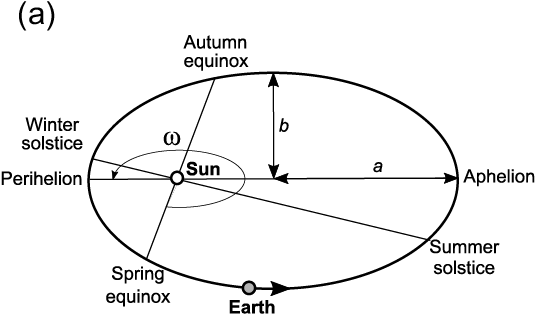
(a) Parameters of the Earth orbit. Here, a is the semimajor and b is the semiminor axis which defines the eccentricity $\text{e}=\frac{\sqrt{{\text{a}}^2-{\text{b}}^2}}{\text{a}}$. The angle between vernal (NH spring) equinox and perihelion $\text{ω}$ is called the climatic precession.

Figure 1.7a long description..

Figure 1.7(a)Long description

Schematic representation of the Earths orbit around the Sun, which is located at one of the focal points of the ellipse. The position of key elements of the orbit: aphelion, perihelion, summer and winter solstices, and spring and autumn equinoxes. The semimajor and semiminor axes of the ellipse determine the eccentricity of the Earths orbit. The angle between the vernal equinox and perihelion is called the climatic precession.

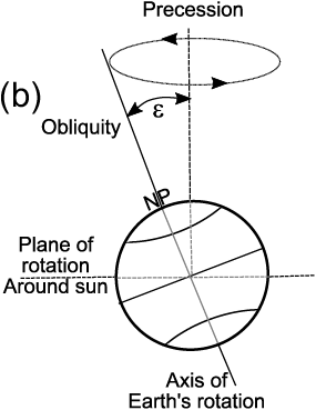
(b) The precession of Earth’s axis with respect to the orbital plane, where $\text{ε}$ is obliquity.

Figure 1.7b long description..

Figure 1.7(b)Long description

Schematic representation of the direction of the Earths axis relative to the plane of rotation of the Earth around the Sun and explains that the angle between the axis and the perpendicular to the plane of rotation is the obliquity.

Precession (more precisely, the precession of the equinoxes) is related to the fact that the combination of the precession of the Earth’s orbit, with a period of 26,000 years, and the rotation of the principal axis of the Earth’s orbit, with a period of about 100,000 years, leads to changes in the position of the summer and winter solstices relative to aphelion and perihelion, with a typical periodicity of about 23,000 years. At present, the boreal (i.e., northern) summer occurs around aphelion (the point on the Earth’s orbit where the planet is at its greatest distance from the Sun), that is, summer insolation is lowest (compared to other positions on the orbit) and therefore summers are colder than average. Twelve thousand years ago, the situation was reversed and the boreal summer occurred at the position closest to the Sun, making summer insolation significantly higher than today. The difference in insolation between perihelion and aphelion is proportional to eccentricity. For a high eccentricity of about 0.05 (see Figure 1.8c), the difference in summer insolation between aphelion and perihelion in the boreal latitudes would be about 50 W/m², or about 20% of its annual mean value. At the same time, precession has virtually no effect on the mean annual insolation at any latitude – it simply redistributes the insolation between the different seasons.

Figure 1.8

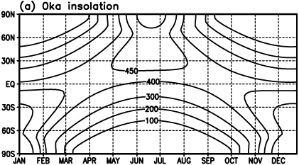
(a) Present daily insolation at the top of the atmosphere in W/m².

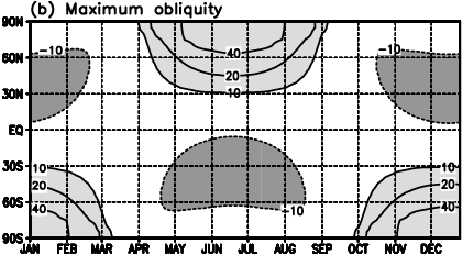
(b) Maximum effect of obliquity on daily insolation (difference between obliquity parameters 24.5° and 22°)Maximum effect of obliquity on daily insolation (difference between obliquity parameters 24.5° and 22°)The maximum effect of obliquity on daily insolation (difference between obliquity parameters 24.5° and 22°).

(c) The maximum effect of precession is calculated for an eccentricity of 0.03 (close to the mean eccentricity value) between the “warm” orbit (summer solstice occurs at perihelion) and the “cold” orbit (summer solstice occurs at aphelion). The effect of precession on the change in insolation is sensitive to the choice of the calendar. The modern calendar (spring equinox on March 20) is used here. Daily insolation is calculated using the Earth’s orbital parameters from Laskar et al. (2004).

Another astronomical factor affecting climate is obliquity, which is the angle between the Earth’s orbital axis and the normal to the plane of the Earth’s rotation around the Sun (the plane of the ecliptic). This angle varies with time, typically in the range of 22°–24.5°, but the magnitude of these variations is not constant. The dominant frequency of these variations is about 41,000 years. Obliquity determines the distribution of isolation between low and high latitudes, as well as the seasonality of climate. The change in obliquity mainly affects insolation at high latitudes. High obliquity implies higher summer and annual insolation at high latitudes in both hemispheres, which is compensated by lower insolation at low latitudes (see Figure 1.8b). The net effect of obliquity on global mean insolation is zero.

1.5.4 Well-Mixed Greenhouse Gases

Although water vapor is the main greenhouse gas in the atmosphere, its concentration varies in space and time and is controlled by the climate itself. For this reason, water vapor is always considered an internal feedback rather than a forcing agent. The next three greenhouse gases – carbon dioxide (CO₂), methane (CH₄) and nitrous oxide (N₂O) – have a relatively long residence time in the atmosphere and therefore their concentrations are almost homogeneous in the free atmosphere. Even for methane, which has the shortest residence time (about ten years), concentrations in the northern and southern hemispheres differ by less than 10%. This is why they are called well-mixed greenhouse gases.

There are ample evidences that changes in atmospheric concentrations of these three greenhouse gases during and before the Quaternary represent one of the most important factors influencing global climate. Continuous and sufficiently accurate records of CO₂, CH₄ and N₂O concentrations are available from Antarctic ice cores for the last 800,000 years. Prior to this period, CO₂ reconstructions have been based on several indirect proxies, but these are much less reliable and often inconsistent. For the other two well-mixed greenhouse gases so far, there are no reconstructions before 800 ka.

Various reconstructions suggest that at the beginning of the Cenozoic (early Eocene, about 60 Ma), the CO₂ concentration was above 1000 ppm, which is at least four times the preindustrial CO₂ concentration, and this was the main factor explaining the warm climates of the Eocene. The decrease in CO₂ concentration during the last 60 Ma explains the general cooling trend of the Cenozoic. The CO₂ concentration just before the Quaternary is not accurately known, but was probably not much higher than 400 ppm.

The mechanisms of past changes in CO₂ are only partially understood. On long time scales (millions of years), atmospheric CO₂ concentrations are controlled by the balance between CO₂ input (mainly through volcanic activity) and CO₂ removal through silicate weathering and burial of organic carbon. Therefore, on geological time scales, CO₂ is treated as an external (to the climate system) forcing. On shorter time scales, such as orbital time scales, CO₂ variations in the atmosphere are primarily due to the redistribution of carbon between atmospheric, oceanic and terrestrial carbon pools. In this case, CO₂ represents a complicated internal feedback (or rather a set of climate-carbon cycle feedbacks). It is important that they are feedbacks to the climate changes driven by the orbital forcing, but not to the orbital forcing itself.

In recent millennia, deforestation was a major anthropogenic source of atmospheric CO₂ but after the beginning of the industrial revolution (nineteenth century), the burning of fossil fuels (coal, oil, gas) became an increasingly the most important contributor to atmospheric CO₂. Currently, the CO₂ flux from fossil fuel combustion exceeds the flux from land use by a factor of five and from volcanic outgassing by two orders of magnitude. The CO₂ concentration is currently rising at about 2 ppm per year and has exceeded 400 ppm by 2015, which is probably the highest CO₂ concentration at any time during the entire Quaternary. Methane and N₂O concentrations are also influenced by human activities and have increased rapidly over the last century. In addition to natural GHGs, there are several other man-made GHGs, such as CFCs.

The radiative forcing of well-mixed greenhouse gases is relatively well known from model simulations. For example, at the LGM, the total radiative forcing of three greenhouse gases relative to the preindustrial state was about −3 W/m². The effect of greenhouse gases on climate is less accurately known due to large uncertainties associated with climate feedbacks. For example, climate sensitivity is still uncertaint and is estimated to be in the range of 2–4.5°C. A number of attempts have been made in recent years to use past climates to better constrain climate sensitivity. Assuming an equilibrium climate sensitivity (ECS) of 3°C (the most likely value according to the 2021 IPCC report), a glacial decrease in well-mixed greenhouse gases can explain about half of the reconstructed 6°C global cooling (Tierney et al. 2020).

1.5.5 Atmospheric Aerosols

Aerosols, solid or liquid particles suspended in the atmosphere, typically of micrometer size, affect the climate in various ways, depending on the size and type of aerosol. The most common type of aerosol is the aeolian dust discussed earlier. It reflects and absorbs solar and infrared radiation. The net radiative effect of dust is usually negative, but the value depends strongly not only on the amount of dust, but also on the minerals, particle size distribution and surface albedo – estimates for the global radiative effect of aeolian dust during the LGM range from zero to several W/m² (Albani et al. 2016). In addition, dust deposited on snow and ice can affect surface albedo and thus not only the global radiative balance, but also the mass balance of continental ice sheets.

Sulfur aerosol mainly reflects sunlight. This aerosol can be formed naturally as a result of volcanic eruptions and has a lifetime ranging from a month to several years. This is enough time for the volcanic aerosol to be distributed across the globe in the stratosphere. The radiative forcing of sulfur aerosol depends on the magnitude of the volcanic eruptions and other factors. During several large volcanic eruptions in the last century, the peak global negative radiative forcing reached several W/m². During catastrophic eruptions, such as Tambora in 1815, the estimated global radiative forcing was about −5 W/m² (Crowley 2000). At present, anthropogenic activities (mainly the burning of fossil fuels) result in the emission of a significant amount of sulfur aerosol, which produces the negative global radiative forcing of about 1 W/m², partially offsetting the warming effect of increasing greenhouse gas concentrations. Black carbon is produced naturally by forest fires and is an absorbing aerosol. A significant amount of black carbon is currently produced by humans.

In addition to the direct radiative effect, some aerosols act as cloud nucleation centers, so their amount affects cloud formation, cloud albedo and precipitation. This indirect effect of aerosols on climate can be of comparable magnitude to their direct effect.

1.5.6 Ice Sheets

Surface albedo strongly influences the Earth’s radiative balance, but changes in surface albedo associated with snow cover or sea ice are not considered as climate forcings, but rather as albedo feedback, which is strongest at high latitudes in both hemispheres. Other changes in surface albedo associated with Quaternary climate variability, such as those caused by the growth and retreat of continental ice sheets, changes in vegetation cover and exposure of oceanic shelves due to changes in sea level, can be considered as forcings when, for example, simulating the climate of the Last Glacial Maximum. At the LGM, the global radiative forcing of the ice sheet is estimated to be 2–3.5 W/m² (Abe-Ouchi et al. 2015), comparable to that of well-mixed greenhouse gases. The important difference in the impact of ice sheets on climate is that the effect of ice sheets on climate is much more localized than that of greenhouse gases. Moreover, ice sheets affect climate not only through changes in planetary albedo, but also through atmospheric and oceanic circulation and changes in sea level. The most direct effect is the additional cooling over ice sheets associated with their high elevation, as the temperature in the free atmosphere decreases with elevation by about 6°C per km. For a typical ice sheet height of 3 km, this should result in a local cooling of about 20°C. At the same time, the growth of the ice sheets leads to a lowering of the sea level, which partly compensates for the elevation-related cooling above the ice sheets. The lowering of the sea level also leads to a reduction in the area of the ocean, and the surface albedo of exposed shelves is higher than that of open water. Furthermore, such a reduction in ocean area also reduces global evaporation, causing additional cooling.

1.6 Climate Feedbacks and Climate Sensitivity

1.6.1 Climate Feedbacks

The concept of climate feedbacks is purely theoretical because feedbacks cannot be observed or measured, but it is very useful for understanding climate change and comparing different climate models. The concept originated in electrical engineering and has spread to various fields of science, including climate science. Positive (negative) climate feedback refers to a chain of processes in the climate system that amplify (attenuate) the initial climate response to a particular climate forcing, such as a change in CO₂ concentration. Sufficiently strong positive feedbacks can destabilize the climate system and lead, for example, to the emergence of multiple equilibria. Negative feedback always stabilize the system. The most important climate negative feedback is the so-called Plank feedback, which is related to the fact that as the temperature increases, so does the long-wave radiation emitted by the planet. On geological time scales, the climate-weathering negative feedback maintains the relative stability of the Earth’s climate necessary to sustain life.

Traditionally, four climate feedbacks are considered to be “fast” (also known as “Charney feedbacks”) and they together determine the important climate characteristic – ECS, defined as the equilibrium response of global surface air temperature to a doubling of CO₂ concentration. These are the water vapor, lapse rate, cloud and albedo climate feedbacks. These feedbacks are relatively fast, that is, they respond on time scales of years to decades, but due to the very large thermal inertia of the deep ocean, it takes several millennia for the surface temperature to reach an equilibrium state. As a result, the strength of individual feedbacks can change over time.

The water vapor feedback is the strongest positive feedback under current climate conditions, and this feedback alone doubles the global temperature response to CO₂ radiative forcing. Although the water vapor feedback is always positive, its magnitude varies considerably between different models. This is because although most of the water vapor is in the lower troposphere, a relatively small amount of water vapor in the upper troposphere plays an important role in the radiative balance of the atmosphere and climate models differ considerably in how they simulate changes in water vapor in the upper troposphere.

The lapse rate feedback is explained by the fact that the lapse rate (the vertical temperature gradient in the atmosphere) tends to decrease with global warming in the tropics and midlatitudes. As a result, the temperature change in the upper troposphere is greater than that near the surface, and the atmosphere therefore emits more longwave radiation compared to a case of uniform atmospheric warming. This effect thus reduces the magnitude of global warming, and is a negative feedback. This feedback largely counteracts the water vapor feedback, except at high latitudes where the lapse rate feedback is also positive. Model results suggest that the sum of the water vapor and lapse rate feedbacks is less uncertain than either feedback separately. This is because a more negative lapse rate feedback leads to more warming in the upper troposphere and thus to a larger increase in water vapor, implying a stronger greenhouse effect of water vapor.

Another positive feedback is the albedo feedback, which was already included in Milankovitch’s calculation of the effect of summer insolation changes on ice sheet growth (Milankovitch 1941). This feedback was also explicitly parameterized in Budyko’s energy balance model (Budyko 1969), and it was shown that this feedback can lead to the emergence of the second equilibrium climate state – the so-called “snowball Earth.” The albedo feedback results from the fact that as the climate warms (cools), the area covered by snow and sea ice decreases (increases). Since the albedos of snow-covered land and sea ice are greater than the corresponding albedos of snow-free land and open ocean, these changes in surface cover amplify the initial temperature response (see Figure 1.9). The albedo feedback is strongly climate-dependent, that is, it is weaker in warm climates and stronger in cold climates. Note that the “fast” (Charney) albedo feedback only accounts for changes in snow and sea ice cover, not changes in ice sheets. The latter are treated separately, as they operate on completely different time scales (see later).

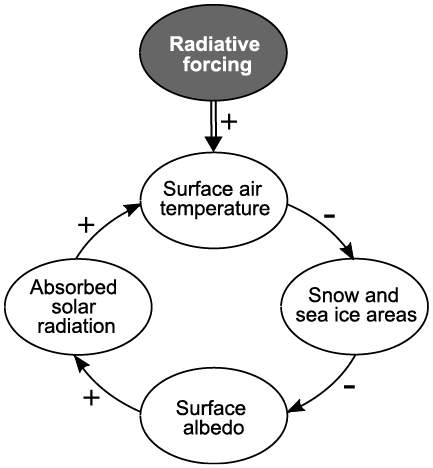
Figure 1.9 Flowchart diagram illustrating the snow and ice albedo feedback loop. An increase in radiative forcing (e.g., due to an increase in atmospheric CO₂ concentration) leads to an increase in surface air temperature, a decrease in the area covered by snow and sea ice, and thus, a decrease in surface albedo. This leads to an increase in absorbed solar radiation and hence additional warming. The albedo feedback is therefore positive. A similar feedback but on longer time scales operates through the continental ice sheets.

Figure 1.9 long description..

Figure 1.9Long description

Flowchart consists of five ellipses. The top ellipse represents the radiative forcing. The other four ellipses, in clockwise order, represent surface air temperature, snow and sea ice cover, surface albedo and absorbed solar radiation. An increase in radiative forcing leads to an increase in surface air temperature (the ellipse below the radiative forcing), which in turn leads to a decrease in snow and sea ice (the right ellipse). The signal propagates clockwise to the surface albedo (lower ellipse), leading to a decrease in albedo. This in turn leads to an increase in absorbed solar radiation (left ellipse). The positive feedback loop is closed by an additional increase in surface air temperature.

The cloud feedback is the most uncertain. The cloud feedback operates through changes in cloud fraction and height, and the optical properties of clouds, which depend on both water content and droplet size. The cloud feedback is very spatially heterogeneous, but in most climate models the cloud feedback is globally positive. Model results also suggest that this feedback may be strongly climate-state dependent, but even the sign of this dependence is not known.

In addition to the four fast (Charney’s) climate feedbacks that determine the ECS, there are other feedbacks that can affect climate on longer time scales. The albedo feedback associated with ice sheets is particularly important for Quaternary climate dynamics. Unlike the fast albedo feedback associated with snow and sea ice cover, the albedo feedback related to ice sheets operates on millennial and longer time scales. In addition, the albedo feedback associated with ice sheets is highly nonlinear, as the transition from ice-free to ice-covered northern continents may represent a bifurcation transition.

Another feedback operating on centennial to millennial time scales is the vegetation feedback. At least in boreal latitudes, this feedback, also known as the taiga–tundra feedback, is positive. Model simulations suggest that changes in vegetation cover during glacial periods may contribute an additional 0.5–1°C to global cooling. Another potentially important feedback is the dust feedback. Model simulations suggest that an increase in dustiness during the glacial period contributed to additional global cooling, but the magnitude of the cooling remains uncertain. There are several feedbacks related to the carbon cycle. Some can be relatively fast (such as the climate-methane feedback), and others, such as the climate-weathering feedback, operate only on geological time scales. The term feedback can be applied not only to temperature but also to other climate properties, and not only at global but also at regional scales. A typical example is the “greening” of the Sahara due to the climate-vegetation feedback (see also Box 7.1).

1.6.2 Climate Sensitivity and Transient Climate Response

ECS can only be obtained from the results of specially designed climate model simulations in which only the atmosphere, ocean and physical components of the land surface are allowed to change, while ice sheets, vegetation cover, soil properties, and so forth are fixed. To determine the ECS in a climate model, it is necessary to run simulations for two different CO₂ concentrations. Such numerical experiments should be long enough to approach equilibrium with the desired accuracy. Typically, such experiments require several thousand model years due to the very long response time of the deep ocean. Since performing such simulations with complex climate models is computationally demanding, the Gregory method (Gregory et al. 2004) is often used to determine the ECS accurately enough from much shorter model simulations. The range of climate sensitivity was first reported about 40 years ago in the so-called “Charney Report” (Charney et al., 1979), where the ECS was estimated to be in the range of 1.5°C–4.5°C. Surprisingly, this range has remained largely unchanged in the following decades. The main reasons for such large uncertainties in this important climate metric are the large differences between the results of different climate models and the lack of good empirical constraints on this property (see Box 1.2). The latest IPCC report (IPCC 2021a), largely based on Sherwood et al. (2020), gives a “likely” range for ECS of 2.5°C–4°C, but a “very likely range” of 2°C–5°C that is twice as wide. The term “very likely range” should not be understood to mean that any value within this range is “very likely,” but that the values outside this range are very unlikely, technically <10% probability.

In addition to the traditional ECS, a more general term called “specific climate sensitivity” is used as a metric for the global temperature response to different types of radiative forcing (Rohling et al. 2015). Specific climate sensitivity is defined as the equilibrium global surface air temperature response to a unit perturbation in global radiative forcing and is measured in (KW⁻¹m² or °CW⁻¹m²). Specific climate sensitivity can be applied to any radiative forcing, not just CO₂, assuming that the global temperature response to the radiative forcing does not depend on the nature of the forcing. Typical estimates of specific climate sensitivity are in the range of 0.5–1.5°CW⁻¹m², which roughly corresponds to an ECS range of 2°C–4.5°C. However, there is no reason why one W/m² of global radiative forcing of different nature (CO₂, solar constant or atmospheric aerosols) should produce exactly the same global temperature response. The difference in the temperature effect of different radiative forcings is characterized by the term “forcing efficacy,” which represents the relative response to a given forcing compared to CO₂ (Hansen et al. 2005).

Since slow climate feedbacks can significantly affect the climate response to radiative forcing on long time scales, it has been proposed to introduce a new term – “Earth System Sensitivity” – which is defined as the equilibrium response to a doubling of CO₂ or other radiative forcing on much longer time scales, in analogy to the ECS, which is driven by fast climate feedbacks. In this case, ice sheets, vegetation and other feedbacks should also be taken into account. The problem with Earth System Sensitivity is that at least some of the slow feedbacks are fundamentally nonlinear, while the time scale of ice sheet response to climate change is so long that the concept of equilibrium response becomes impractical. Nevertheless, when considering long-term scales, it is important to remember that the climate response to different types of external forcing is not only determined by fast climate feedbacks and may therefore be stronger than those calculated by climate models, which typically only consider fast climate feedbacks.

On shorter time scales (decadal to centennial, relevant to the Anthropocene), the climate system is far from equilibrium with the concentration of CO₂ and other greenhouse gases, whose radiative forcing is currently increasing at a rate of 0.5% per year. To characterize such a nonequilibrium response of the climate to radiative forcing, another metric, the Transient Climate Response (TCR), is defined as the global temperature rise at the time of CO₂ doubling in the scenario where CO₂ increases at the rate of 1% per year from the preindustrial value, that is, about 70 years after the start of the model experiment. Due to the large inertia of the ocean, the climate system is out of equilibrium with the CO₂ concentration and the TCR is typically only 50–60% of the ECS. Although the TCR is not solely determined by the ECS, these two characteristics are generally well correlated (Meehl et al. 2020), implying that climate models with higher ECSs tend to produce higher global warming, regardless of the specific CO₂ scenarios.

1.7 Elements of Dynamical Systems Analysis

The terminology of dynamical systems theory (or analysis), such as stability, multiple equilibria, bifurcation transitions, and so forth, is widely used to discuss the evolution of the Earth system and its response to different forcings. Needless to say, the real Earth system is incomparably more complex than the mathematical models (usually based on several ordinary differential equations) studied in dynamical systems theory. Nevertheless, this terminology is useful, although it needs to be clearly defined in each specific case, and the limits of its applicability should be assessed.

1.7.1 Existence of an Equilibrium State and Stability

The basic premise of climate dynamics is that the preindustrial climate was a quasi-equilibrium and stable climate state. “Quasi-equilibrium” in this context means that, due to intrinsic internal variability, climate characteristics such as annual mean surface air temperature vary in time, but on longer time scales (centennial to millennial) no significant trends in different climate variables have been detected, at least on a global scale. This allows us to clearly distinguish between different climatic conditions, such as the cold climate of the Last Glacial Maximum or the warm climate of the Late Pliocene. The term “stable” is used in climatology in two different senses. The first is not related to external perturbations, but rather characterizes qualitatively the extent of natural variability and trends. In this sense, a stable climate is one characterized by low variability, and this term is often applied to the Holocene climate. The glacial climate, on the other hand, is characterized by strong internal variability and can be considered “unstable.” Another meaning of “stability,” as used in dynamical systems theory, is that the response of the system to a small external perturbation is also small, and once the perturbation is removed, the system returns to its initial state after a characteristic time. This would also imply that the system response to a small perturbation is “reversible.” The results of experiments with climate models seem to support the idea that the current (i.e., preindustrial) climate state is stable and that the system response to small external perturbations (CO₂, solar constant, etc.) is quasi-linear. However, this is only true for climate models that do not include ice sheets, because interactive ice sheets can cause a strong discontinuity in the state of the Earth system close to the preindustrial state associated with the onset of large-scale glaciation of the Northern Hemisphere.

1.7.2 Multistability, Instability and Bifurcation Transitions

In general, it is possible that a sufficiently large perturbation can move the system to a different stable equilibrium, such that after the perturbation is removed the system will not return to its original state, that is, the change would be irreversible. The transitions between different climate states are usually interpreted in terms of bifurcation transitions, and the critical values at which such transitions occur are associated with the bifurcation points (see Figure 1.10a). Bi-stability can also be represented in the form of a two-well diagram. In this case the stability can be characterized by the “depth” of the corresponding well. For example, in the case shown in Figure 1.10b, both equilibria are stable, but EI is less stable and a relatively small perturbation, or just a random forcing of sufficient magnitude, can move the system from equilibrium state EI to state EII.

Figure 1.10

(a) A typical stability diagram of a nonlinear system with multiple equilibrium states in the phase space of a forcing. EI and EII are two different stable equilibrium states, UE is an unstable equilibrium, BI and BII are bifurcation points where the transitions between two equilibrium states occur. The gray area depicts the domain of attraction of state EI; the white area is the domain of attraction of state EII.

Figure 1.10a long description..

Figure 1.10(a)Long description

Figure shows the stability diagram of a bistable system in the phase space of the external forcing. The top and bottom curves in this figure show two stable equilibria separated by an unstable equilibrium. The vertical arrows show the transitions between the two equilibrium states.

(b) Illustration of the bistable system using a potential well diagram. Changes in the forcing can cause transitions between two states. Similar stability diagrams have been found for simple Budyko-type, energy balance model, the AMOC in freshwater space, or climate-cryosphere system in the phase space of orbital forcing.

Figure 1.10b long description..

Figure 1.10(b)Long description

Figure shows the stability diagram for the same system using a potential well diagram. This diagram is represented by a graph with two minima, each representing a stable equilibrium. The system, depicted by a ball, is located in one of the potential wells, but can be pushed into another one by the external forcing indicated by a horizontal arrow.

A number of such possible equilibrium states have been identified in modeling studies. The most dramatically different from the present is “snowball Earth,” where the entire planet is covered in ice and the global surface temperature is more than 40°C below the present value (see also Chapters 3 and 4). Another cold climate state found in models is the state where the northern part of North America and Eurasia are covered by thick ice sheets, but the rest of the planet (apart from Antarctica) remains ice-free and relatively warm (see also Chapter 5). Both states in the models can exist under the external forcing and boundary conditions of modern climate (CO₂ concentration, insolation, Earth’s geography), but they differ significantly in the magnitude of the perturbation required to move the Earth system into these states. According to model simulations, the transition to the snowball states requires a reduction in the solar constant of about 10%, while the trigger for the onset of glaciation (partial glaciation of the northern continents) is only about 1%. Modeling studies also suggest that two possible states of the AMOC – the so-called AMOC-on and -off – can coexist within a certain range of forcing or climate conditions (see also Chapter 6), but the question of whether the AMOC has multiple equilibria under present climate conditions remains controversial. The situation is similar for the Greenland and West Antarctic ice sheets. Models suggest that they could disappear completely under climate conditions that are only moderately warmer than today, but it is not clear whether they are bistable, for example, under preindustrial conditions. In general, if the system is close to such a bifurcation point, it can be considered unstable. However, instability can also take other forms. For example, a reduction in CO₂ below a certain threshold leads to the appearance of strong millennial-scale variability in some climate models, similar to the observed Dansgaard–Oeschger events.

The possibility of the existence of multiple equilibria poses a serious problem for climate modeling. Indeed, in the case of multiple equilibria, it is possible that the equilibrium state that the model will reach under constant external conditions will depend on the initial conditions. Since the initial conditions of the Earth system are never known with absolute precision, it is impossible to rule out the possibility that the model will end up in the “wrong” equilibrium state.

1.7.3 Chaos and Predictability

When discussing the modeling of long-term climate evolution, either future or past, the question of chaotic behavior of the Earth system and thus the possibility of climate predictability naturally arises. The problem can be formulated as follows: “The climate system is a coupled nonlinear chaotic system, and therefore long-term prediction of future climate states is not possible (IPCC 2007).” However, the interpretation of this statement depends on what is meant by long-term climate prediction.

The limited predictability of weather is explained by the fact that even very small differences in initial conditions inevitably lead to a divergence in predictions, and after a certain time the difference between different simulations diverges too much to be useful as a forecast. For the weather, the limit of predictability is about a week, but for some aspects of climate variability, such as ENSO, a useful forecast is in principle possible for at least half a year. The long memory of the ocean gives hope for some useful predictions even on the decadal time scale. On longer time scales, anthropogenic forcing becomes the dominant factor in expected climate change. As a result, climate predictability, expressed in terms of the signal-to-noise ratio, initially increases with time. However, in the second half of the present century, future CO₂ and other anthropogenic emission scenarios diverge strongly, and uncertainties in future anthropogenic forcing become the dominant source of uncertainty in future climate projections, although inter-model differences also play a significant role. However, these large uncertainties in climate projections are not related to the chaotic nature of the climate system.

In modeling past climate change, the projection becomes the hindcast, and the question of whether the climate is deterministic or chaotic can be formulated as follows. Assuming that the key external forcing(s) and boundary conditions are known with sufficient accuracy, the question is whether it is possible to simulate past climates with sufficient accuracy even if the initial conditions required for such simulations are not well known. The situation is likely to be very different for different types/modes of climate variability. In the case of glacial cycles (both past and future), the orbital forcing is well known and, based on previous modeling studies, it appears possible to reproduce not only the main statistical properties of glacial cycles, such as periodicity and amplitude, but also the precise timing of these cycles. For example, in the absence of anthropogenic forcing, the onset of the next glacial cycle is expected to occur 50 kyr from the present. Of course, it cannot be ruled out that such predictability is only partial and that chaotic (random) processes will cause divergence in possible climate trajectories. However, such divergence is not necessarily monotonic and the results of different simulations may converge again.

The situation is different for millennial-scale climate variability, such as the Dansgaard–Oeschger and Heinrich events. Millennial-scale variability is a prominent feature of Quaternary climate dynamics, but it is very likely that it has no external forcing and thus arises solely from the internal instability of the Earth system. In such a case, it is still possible for models to simulate such variability correctly in terms of the statistical properties of such events, but since the timing of individual events is random, the probability that the timing of simulated events will coincide with that of the recorded millennial-scale variability is essentially zero. For example, a sequence of warm and cold events during the last deglaciation, similar to the real Bølling–Allerød and Younger Dryas events, can in principle be simulated with the models. However, their timing is unlikely to be close to the real events.

Box 1.1Orbital Forcing

The spatial and temporal distribution and variation of insolation is the main factor that determines climate. The insolation at the top of the atmosphere at any given location at any given time can be calculated as

$I=S_0{\left(\frac{r_0}{r}\right)}^2\text{cos}\xi ,$

where S₀ is the “solar constant,” the average solar energy flux per square meter at the average distance of the Earth from the Sun r₀, and r is the actual distance from the Sun, $\text{ξ}$ is the so-called zenith angle, that is, the angle between the Sun and the zenith. This angle is computed by the formula

$\text{cos}\zeta =\text{sin}\phi \text{sin}\delta +\text{cos}\phi \text{cos}\delta \text{cos}\Psi ,$

where $\phi$ is the latitude, $\delta$ is the solar declination, which is the angle between the Sun and the equatorial plane of the Earth, and $\text{Ψ}$ is the hour angle. The values of r and $\delta$ depend on precession, eccentricity and obliquity, and the time of year (season), while $\text{Ψ}$ depends on the time of day, being the angle between the current position of the Sun and the direction to the noon.

Accurate calculations of the temporal evolution of insolation over the past 600 kyr were made by Milutin Milankovitch more than a hundred years ago. At that time, the calculations were very laborious and he made them only for a few latitudes. Nowadays, all climate models include fairly efficient numerical algorithms for calculating solar radiation at any time and place, which take a negligible amount of computing time. Calculations of insolation require accurate knowledge of the three orbital parameters, which are now calculated for the past and future 50 million years (Laskar et al. 2011).

In developing his theory, Milankovitch adopted the already proposed idea that changes in boreal summer insolation are critical for understanding ice ages. As a measure of summer insolation, Milankovitch used the integral of insolation during a warm (caloric) half year. In post-Milankovitch times it became common to use June or July insolation at 65°N (see, e.g., Berger 1978), although caloric half year insolation is still used in some papers. When discussing which single metric best represents the orbital forcing, it is important to recognize that climate models calculate insolation at every time step and for every grid cell, and therefore climate modelers do not need to decide which definition of “summer insolation” is the best. However, for analysis of paleoclimate records and construction of simple (conceptual) models of glacial cycles, it is desirable to convert three-dimensional daily insolation (latitude – day of year – year before or after present) into a single metric. Figure 1.11 shows both metrics for orbital forcing – maximum and caloric half-yearly insolation at 65°N. As can be seen from comparison of their frequency spectra, the main difference between these two metrics is the relative contribution of precession and obliquity. The maximum insolation is dominated by precession, whereas for the half year insolation these two components are of comparable importance. Thus, regardless of which of the two metrics is considered the best for orbital forcing, one would expect to see both precession and obliquity components in the case of a linear response of the system to orbital forcing. The appearance of eccentricity frequencies requires the Earth system response to orbital forcing to be nonlinear, and the dominance of a single eccentricity frequency in the spectrum of the late Quaternary climate variability requires a very specific type of non-linearity (Ganopolski 2024).

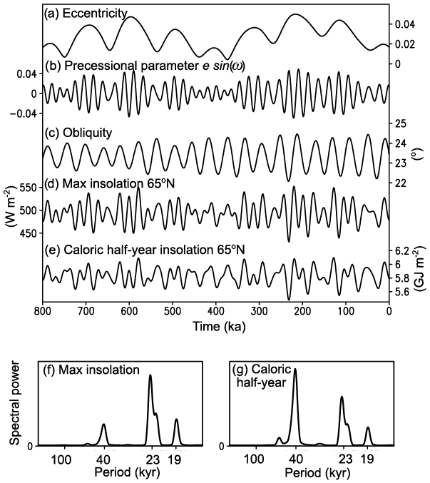
Figure 1.11 Earth’s orbital parameters, two most common proxies for orbital forcing, and their frequency spectra. (a) Eccentricity; (b) precessional parameter $e\hspace{0.33em}\sin (\omega )$; (c) obliquity; (d) maximum summer insolation at 65°N in (W/m²); (e) caloric summer half year insolation at 65°N (in GJ m⁻²); (f) frequency spectrum of maximum summer insolation at 65°N; and (g) frequency spectrum of caloric summer half year insolation at 65°N. Frequency spectra are in arbitrary units.

Modified from Ganopolski (2024).

Box 1.2Using Paleoclimate Data and Modeling to Constrain Climate Sensitivity

Climate sensitivity is an important metric of the response of the climate system to perturbations in radiative forcing, but despite numerous efforts to constrain it, climate sensitivity remains highly uncertain (Sherwood et al. 2020). While the first estimate of the ECS was based on the results of just two rather simplistic climate models available in the mid 1970s, there are now several dozen different complex climate models that simulate today’s climate much better than the previous generation of climate models. Nevertheless, similar to previous generations, modern climate models produce ECSs that are relatively uniformly distributed between 2°C and 5°C (Meehl et al. 2020), that is, mostly within the original Charney range.

The observed climate change over the last 100 years is well known, but due to large uncertainties in the total climate forcing (mainly due to the aerosol component) and the oceanic heat uptake, it difficult to accurately derive the ECS from observational data alone. Therefore, a number of attempts have been made to use paleoclimate data in conjunction with climate modeling to reduce these uncertainties. Most of these studies have used Quaternary paleoclimate reconstructions, although some have also used data from the deep past. There are several approaches to using paleodata for this purpose.

The first requires only knowledge of the global mean surface air temperature anomaly $\text{Δ}{\text{T}}_{\text{g}}$ and the total radiative forcing anomaly $\text{Δ}{\text{R}}_{\text{g}}$ relative to the preindustrial climate state (Hoffert and Covey 1992). Then, assuming that the climate was in a quasi-equilibrium state, the so-called “specific climate sensitivity” can be calculated as

$S=\frac{\text{Δ}{T}_g}{\text{Δ}{\text{R}}_g},$

where global mean radiative forcing $\text{Δ}{\text{R}}_g$ in the case of any Quaternary climates cane be calculated as the sum of several individual climate forcings:

$\Delta R_g=\Delta R_{GHG}+\Delta R_I+\Delta R_{LO}+\Delta R_V+\Delta R_D.$

Here $\Delta R_{GHG}$ is the radiative forcing due to changes in the concentrations of CO₂, CH₄ and N₂O, $\Delta R_I$ is the radiative forcing due to continental ice sheets, $\Delta R_{LO}$ is the radiative forcing due to changes in land area (land albedo is lower than ocean albedo, and therefore sea level fall due to ice sheet growth leads to an increase in planetary albedo), $\Delta R_V$ is the radiative forcing due to changes in vegetation cover and $\Delta R_D$ is the radiative forcing due to changes in aeolian dust. It is important to note that this approach is explicitly based on the assumption that radiative forcings of different origin have the same effect on global temperature (i.e., have the same efficacy), which is not an obvious assumption. The ECS can then be calculated from the specific climate sensitivity as

$ECS=\Delta T_{2\times CO2}=S \hspace{0.17em}\hspace{0.17em}\Delta R_{2\times CO2},$

where $\Delta R_{2\times CO2}$ is the radiative forcing of CO₂ doubling. Although the motivation for estimating ECS from paleodata is to obtain ECS independent of climate models, climate models are still required to estimate ECS with paleoclimate data. First, individual components of the radiative forcing can only be calculated from model simulations. Second, reconstructing global temperature change from paleoclimate data alone is also problematic. Paleotemperature reconstructions are rather sparse, and there are some regions where they are simply not available, such as the ice sheets that do not exist today, or areas covered by sea ice for most of the year. Although even in the LGM ice sheets and sea ice covered only 10% of the Earth’s surface, they were responsible for a much larger fraction of global cooling. Estimates of the total radiative effect of greenhouse gas change, ice sheets, land surface, vegetation and dust based on modeling results are rather uncertain and vary between −6 W/m² and −12 W/m². Combined with the likely range of global LGM cooling from –4°C to −8°C, this gives a range of specific climate sensitivity of 0.3–1.3°CW⁻¹m². Multiplying this value by the radiative forcing estimate for the CO₂ doubling of 3.7 ± 0.8 W/m² gives an LGM-based estimate of the ECS of 1°C–5°C, which is not very different from the Charney range.

Another approach is based on using of results from different climate models or an ensemble of a single model realizations obtained by perturbing key model parameters (so-called “perturbed physics ensemble”). When applying results from different models or model realizations to the LGM, it can be expected that the models with the best fit to the data, are likely to have the “right” ECS. Indeed, results obtained with model ensembles produced from the same model using the perturbed physics approach do show high correlations between ECS and regional LGM cooling (such as tropical SST cooling), and suggest that the models with medium ECS tend to be in a better agreement with the paleoclimate data (Schneider von Deimling et al. 2006). However, this is not the case for the model ensemble consisting of different models (such as those participated in PMIPs) which show very low correlations between ECS and LGM climate change (Renoult et al. 2023).