


1. Introduction
Peru is home to approximately 70% of the world’s tropical glaciers, which are rapidly melting due to climate change. The lack of knowledge regarding ice volume and bedrock topography poses challenges for predicting glacier changes and the associated runoff, as well as the impact of potential glacier dynamical changes on the interpretation of ice core-derived paleoclimate histories. Despite the glaciers’ critical importance as water reservoirs, limited number of published ice thickness measurements exist in Peru (Thompson and others, Reference Thompson, Bolzan, Brecher, Kruss, Mosley-Thompson and Jezek1982, Reference Thompson, Mosley-Thompson, Bolzan and Koci1985, Reference Thompson, Mosley-Thompson, Davis, Porter, Kenny and Lin2018; Peduzzi and others, Reference Peduzzi, Herold and Silverio2010; Salzmann, Reference Salzmann2013).
The spatial variation in ice thickness and basal topography are key parameters for numerous glacio-hydrological applications, including ice volume estimation (Navarro, Reference Navarro2014; Kutuzov and others, Reference Kutuzov, Lavrentiev, Smirnov, Nosenko and Petrakov2019), modeling future glacier dynamics (Zekollari and others, Reference Zekollari, Fürst and Huybrechts2014), hydrological projections (Gabbi and others, Reference Gabbi, Farinotti, Bauder and Maurer2012), hazard studies and glacial lake formation (Vincent and others, Reference Vincent, Thibert and Gagliardini2015; Lavrentiev and others, Reference Lavrentiev, Petrakov, Kutuzov, Kovalenko and Smirnov2020; Ekblom Johansson and others, Reference Ekblom Johansson, Bakke, Støren, Gillespie and Laumann2022), and ice-core analysis (Eisen and others, Reference Eisen, Nixdorf, Keck and Wagenbach2003), among others. Ice thickness measurements, however, are scarce due to logistical challenges, particularly for remote and high-altitude glaciers.
In the absence of observational data, several approaches have been developed to model glacier-wide ice thickness using surface topography, mass balance, ice flow velocities, and theoretical assumptions. However, these estimates have significant uncertainties. It was shown that the mean deviation between the average model composites and the measured ice thickness is on the order of 10 ± 24% of the mean ice thickness while local modeling errors often exceed the observed ice thickness (Farinotti, Reference Farinotti2017). Recent model comparisons reveal inconsistencies, particularly for ice caps, and emphasize the need for improved glacier outlines and detailed glacier ice thickness data to calibrate and validate models (Farinotti, Reference Farinotti2021; Millan and others, Reference Millan, Mouginot, Rabatel and Morlighem2022; Frank and Van Pelt, Reference Frank and Van Pelt2024). Existing ice thickness estimates for glaciers outside the polar ice sheets exhibit major inconsistencies between the modeled results and measurements (Farinotti, Reference Farinotti2019; Millan and others, Reference Millan, Mouginot, Rabatel and Morlighem2022). As a result, assessments of ice volume in the low latitudes vary greatly, from 0.07 ± 0.04 103 km3 to 0.10 ± 0.03 103 km3 (Millan and others, Reference Millan, Mouginot, Rabatel and Morlighem2022), and are highly uncertain for specific watersheds. The accuracy of model estimates relies heavily on the availability and distribution of ice thickness data, which are lacking for the majority of these glaciers. Thus, additional measurements of ice thicknesses in the Peruvian Andes would improve assessments of water storage and aid in the interpretation of paleoclimatic histories preserved in ice cores recovered from the region (Millan and others, Reference Millan, Mouginot, Rabatel and Morlighem2022).
Ground-penetrating radar (GPR) stands as a widely applied geophysical technique in numerous glaciological investigations, including measurement of ice and snow thickness and the assessment of the glacier’s internal structure (Navarro and Eisen, Reference Navarro, Eisen, Pellikka and Rees2009). The integration of GPR into mountain ice coring research has been carried out in the European Alps (Eisen and others, Reference Eisen, Nixdorf, Keck and Wagenbach2003; Licciulli and others, Reference Licciulli, Bohleber, Lier, Gagliardini, Hoelzle and Eisen2020), Tibet (Kutuzov and others, Reference Kutuzov, Thompson, Lavrentiev and Tian2018), Kilimanjaro (Bohleber and others, Reference Bohleber2017), and the Caucasus (Mikhalenko, Reference Mikhalenko2015) among other locations. Information about bedrock topography and englacial layering is used for selecting suitable ice-core drilling sites and interpreting ice-core records (Konrad and others, Reference Konrad, Bohleber, Wagenbach, Vincent and Eisen2013). Internal reflections are believed to originate from layers initially formed on the glacier surface. These isochronal layers play a crucial role in connecting separate ice-core records, estimating accumulation distribution, and calibrating age/depth relationships (Bohleber and others, Reference Bohleber2017; Pälli, Reference Pälli2002; Konrad and others, Reference Konrad, Bohleber, Wagenbach, Vincent and Eisen2013; Sold and others, Reference Sold, Huss, Eichler, Schwikowski and Hoelzle2015; Lavrentiev and others, Reference Lavrentiev, Kutuzov, Mikhalenko, Sudakova and Kozachek2022). High-frequency GPR is also widely used to measure spatiotemporal variations in snow accumulation on glaciers, thus enabling extensive data collection in a short amount of time (McGrath, Reference McGrath2018).
Long-term proxy climate records from ice cores in high-elevation tropical ice caps and polar ice sheets provide essential context for assessing recent climatic and environmental variations and their impacts on human activities (Thompson, Reference Thompson1995). The 1993 Huascarán ice cores provided a valuable record of Late Glacial Stage (LGS) conditions, the LGS-Holocene transition, and the Younger Dryas cooling event in the tropics, and greatly improved our understanding of tropical sensitivity to global climate changes (Thompson, Reference Thompson1995; Davis and Thompson, Reference Davis and Thompson2006; Liu, Reference Liu2023). Achieving reliable modeling of the age/depth relationship and its spatial variation requires accurate ice thickness and bedrock topography data (Eisen and others, Reference Eisen, Nixdorf, Keck and Wagenbach2003; Konrad and others, Reference Konrad, Bohleber, Wagenbach, Vincent and Eisen2013; Licciulli, Reference Licciulli2018; Licciulli and others, Reference Licciulli, Bohleber, Lier, Gagliardini, Hoelzle and Eisen2020). Accumulation zones in high mountains are often characterized by complex three-dimensional flow dynamics and variable snow accumulation patterns. These factors can impact the interpretation of ice cores and require thorough assessment (Lüthi and Funk, Reference Lüthi and Funk2000; Licciulli and others, Reference Licciulli, Bohleber, Lier, Gagliardini, Hoelzle and Eisen2020).
Here we present the results of glaciological and geophysical surveys conducted during the July–August 2019 expedition to Nevado Huascarán, where four ice cores were extracted from the col and on the summit. We describe the methods employed and the data collected during the expedition and discuss the implications of these findings for ice-core interpretations. Additionally, we use this data as input for a 3D full Stokes ice-flow model. The primary goal of ice flow modeling at the Huascarán col drill site is to assess the potential upstream effects and establish a spatial depth/age relationship to verify the optimal placement of the drill sites and to demonstrate the potential application of the geophysical data.
2. Materials and methods
2.1. Ice-core drilling and data collection at Huascarán
Mount Nevado Huascarán, the highest mountain in Peru and the tropics, is located in the Cordillera Blanca of the central Andes (Figure 1). It has two main peaks: Huascarán Norte (6655 m a.s.l.) and Huascarán Sur (6768 m a.s.l.), separated by a saddle or col (6010 m a.s.l.). The saddle-shaped glacier is surrounded by steep icefalls 500 m from the ice divide outflowing to NE and SW and inflowing from NW and SE.
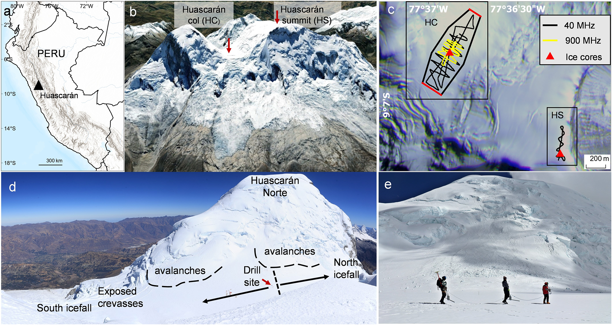
Figure 1. (a) Location of the mount Nevado Huascarán; (b) location of the two drill sites, google earth, image © 2024 airbus; (c) the location of the 40 MHz and 900 MHz GPR profiles near the drill sites is indicated, along with the model domain at HC site, the north and south boundaries are highlighted in red. image © 29 July 2019 planet labs PBC; (d) panorama showing the col of Huascarán from the slopes of Huascarán Sur; (e) geophysical survey at the Huascarán col using 40 MHz frequency antennas.
Huascarán glaciers have been studied using various methods, such as ice cores, remote sensing and surface mass balance (Thompson, Reference Thompson1995). However, there is still a lack of knowledge about the internal structure, temperature regime, ice thickness and flow velocities especially at the ice-core drilling sites. The suitability of the col drill site was established from data collected during previous field seasons (Thompson, Reference Thompson1995; Davis and Thompson, Reference Davis and Thompson2006), including shallow firn-core samples collected in 1991 and 1992; snow-pit samples collected in 1991, 1992 and 1993; and two deep ice cores recovered to bedrock in 1993: HC-93-1 (160.3 m) and HC-93-2 (165.6 m) (Thompson, Reference Thompson1995).
The 2019 expedition to Huascarán successfully recovered four ice cores to bedrock. Two of the cores (HC-19A (165 m) and HC-19B (167.5 m)) were extracted from the Huascarán col (HC), the same site that was drilled in 1993. Two additional cores (HS-19A (69 m) and HS-19B (67.9 m)) were retrieved from the Huascarán summit (6768 masl). The ice cores from the summit are the highest elevation ice cores ever retrieved from the tropics.
During the 2019 campaign detailed glaciological and geophysical surveys also were conducted across the Huascarán col and summit. These measurements include surface snow properties, GPR survey, englacial temperature profiles, and density profiles from snow pits and four ice cores drilled to bedrock.
2.2. Ice core and snow pit sample analysis
Ice cores and snow pit samples were transported frozen to the Byrd Polar and Climate Research Center (BPCRC) at the Ohio State University where they are stored in a −34°C freezer. Each core was subsampled using the procedure described by Weber and others (2023). Samples were analyzed for δ18O and δD using a Picarro L2140-i and for ions and microparticle concentrations in a Class 100 Clean Room at the BPCRC. Ions were measured with a Dionex ICS 5000 while the microparticle concentrations and size distributions were determined with a Beckman Coulter Multisizer 4.
Timescale Reconstruction for 1993 Huascarán col core HC-93-2 was achieved based on a combination of methods (Davis and Thompson, Reference Davis and Thompson2006). Annual counting was possible back to 1720 ± 5 CE for the upper 125 m. Annual counting was later confirmed and extended to 2019 (Weber, Reference Weber2022). Age-depth relationship for the Holocene was developed based on δ18Oair measurements with the estimated uncertainty of ∼600 years at 8 kyr BP. It was shown that ice layers located 2–4 m from the bedrock were formed 11.2-8.2 kyr BP. The lowest 2 m of the HC-93-2 were dated by matching the δ18O record with the δ18O from a tropical North Atlantic marine core resulting in 19 kyr Huascarán col ice-core record (Davis and Thompson, Reference Davis and Thompson2006). For model comparison we use the timescale of the HC-93-2 core extended to 2019 by counting annual layers in the HC-2019-B core.
2.3. GPR ice thickness measurements
For ice thickness measurements at the Huascarán col and summit areas we used a high-performance GPR system manufactured by Geophysical Survey Systems Inc. (GSSI) with a SIR-4000 control unit and 40 and 900 MHz frequency antennas. Data were collected in continuous time mode 22 scans s−1. GPS coordinates were recorded simultaneously using conventional GPS with the nominal horizontal positioning accuracy of ±5 m. The GPR was carried manually by a three-person foot-train on the glacier surface. The 40 MHz frequency antennas were positioned 30–40 cm above the surface. The antennas were arranged parallel to each other and perpendicular to the profiling direction. The GPR was moved at roughly 0.5 m s−1. Positioning data were used to perform the necessary elevation and distance corrections to the GPR profiles. A GSSI model 3101, 900 MHz bistatic antenna was dragged on the snow surface to profile the upper ∼5 m of snow and firn. We collected 5.8 km of 40 MHz profiles at the HC site and 1.3 km at the HS site. A total of 2.3 km of 900 MHz profiles were collected at the col to evaluate the spatial distribution of snow accumulation.
Radar data (radargrams) were processed using Radan 7 software. Post-processing steps involved bandpass filtering, stacking for signal-to-noise ratio enhancement, a Hilbert transformation (magnitude only) to simplify complex horizon waveforms, and single velocity migration for time/depth conversions (e.g. Campbell and others, Reference Campbell, Roy, Kreutz, Arcone, Osterberg and Koons2013; Kutuzov and others, Reference Kutuzov, Thompson, Lavrentiev and Tian2018). Data visualization was performed using open-source GPR software GPRPy (Plattner, Reference Plattner2020). Profiles were digitized manually using the layer-picking mode to select the reflection arrival time from the ice/bed interface. The two-way travel time was then converted into ice thickness depending on the radio wave velocity. Reflection picks were exported to text format for further implementation in GIS.
For both frequencies we used the relationship determined by Kovacs and others, (Reference Kovacs, Gow and Morey1995) to calculate the radio wave velocity and to account for the density dependence of the electric permittivity, ε, of ice and firn:
 \begin{equation}
\unicode{x03B5} = (1 + 0.000845{\unicode{x03C1}})^{2}
\end{equation}
\begin{equation}
\unicode{x03B5} = (1 + 0.000845{\unicode{x03C1}})^{2}
\end{equation}where the density ρ is in kg m−3.
For 40 MHz antennas, the permittivity ɛ was calculated for the upper 40 m using equation (1) and a third-order polynomial approximation of the density profile obtained from ice-core analysis. The mean radio wave velocity (u) was then computed as u = cɛ−0.5 where c is the speed of light. Below 40 m depth, we used a constant velocity of 0.168 m ns−1.
The intersection differences in ice thicknesses were analyzed to estimate radar data quality (Kutuzov and others, Reference Kutuzov, Thompson, Lavrentiev and Tian2018). At 38 intersection points at the HC and 10 points at the HS we found an average ice thickness difference of 1.8% for the col and 2.1% for the summit. A 2% uncertainty was assumed for both sites to account for spatial variations of the radio wave velocity based on ice-core analyses and borehole temperatures. The timing error related to GPR resolution was 2.1 m. The error related to misinterpretation of bed reflections cannot be estimated. To minimize such errors, we avoided picking in the tracers with unclear reflections and used neighboring and cross-profiles to validate bedrock reflections. Total GPR ice thickness measurement error was calculated for each data point, yielding mean values of 5.5 m (3.4%) for HC and 1.8 m (2.5%) for HS sites.
The ice thickness distribution at both sites was mapped by interpolating the ice thickness measurements using the ‘Topo to Raster’ tool based on the ANUDEM algorithm (Hutchinson, Reference Hutchinson1989). We used 30 m resolution NASADEM (NASA JPL, Reference JPL2020) for the topographic corrections and bedrock elevation calculations.
2.4. Ice flow modeling
The velocity field for the HC is simulated based on a 3D full Stokes ice-flow model with a firn rheological law (Gagliardini and Meyssonnier, Reference Gagliardini and Meyssonnier1997). The model is implemented using the finite element software Elmer/Ice (Gagliardini, Reference Gagliardini2013). We performed a steady-state simulation with fixed glacier geometry. The mathematical formulation of the ice-flow problem follows Zwinger and others, (Reference Zwinger, Greve, Gagliardini, Shiraiwa and Lyly2007) and includes the Stokes and the volume balance evolution equations, the stress-free surface boundary condition, and the no-slip bedrock boundary condition (Figure 1c). Unlike Zwinger and others, (Reference Zwinger, Greve, Gagliardini, Shiraiwa and Lyly2007), we used only dynamical equations and did not consider thermo-mechanical coupling with the constant rate factor A = 1.131 × 10⁻²⁴ Pa–3 s–1 considering the average measured borehole ice temperature of ∼–4°C. Model details and parameters are presented in Appendix 1.
Since the GPR data covered only part of the glacier bedrock, the computational domain was restricted to this area, and the lateral boundary connecting the surface and the bedrock boundaries was a fragment of a cylindrical surface (vertical wall). As the lateral boundary was not a physical boundary in the glacier we consider the flow of ice/firn through it. The boundary conditions at the northern and southern margins are not known. The increased slopes up to 15° lead to formation of crevasses at the distance of ∼100 m from the model domain margins. We assumed zero-stress boundary conditions (icefalls). No outflow at the eastern and western side where the slopes of Huascarán summits are situated are assumed based on flat surface topography along the margins.
The age of the ice was calculated using a passive tracer field method according to a derived velocity field (Zwinger and others, Reference Zwinger, Greve, Gagliardini, Shiraiwa and Lyly2007; Gagliardini, Reference Gagliardini2013; Licciulli and others, Reference Licciulli, Bohleber, Lier, Gagliardini, Hoelzle and Eisen2020). The flow enhancement factor E was adjusted to match the ice age distribution curve at the drill site. Backward trajectories from the drill sites were calculated using the Runge–Kutta integrator implemented in the stream tracer of ParaView (Ahrens and others, Reference Ahrens, Geveci and Law2005) to evaluate potential upstream effects. Model results were visualized using ParaView. We inferred the modeled accumulation distribution by converting the depth of the layer with an age of 1 year to m w.e. using the density measured at the drill site.
Additionally we used a one-dimensional two-parameter model (2p-model; Bolzan, Reference Bolzan1985) to estimate age-depth relationship based on available data points. This simple analytical expression describes the thinning of annual layers with depth depending on the mean annual net accumulation rate b (1.54 i.e.) and the thinning parameter p (1.219). We assume constant accumulation over time. The model was fitted with the depths of known ages using the least squares approach.
3. Results
3.1. Borehole temperature and density
Borehole temperature measurements were carried out in 1993 and in 2019, although the 1993 measurements may be affected by the alcohol-water eutectic mixture that was used to keep the hole open during drilling (Thompson, Reference Thompson1995). The 1993 measurements were therefore excluded from the analysis. In 2019, we measured temperatures in the col A borehole using a thermistor that was calibrated to a precision of 0.1 °C. At a given depth, the thermistor equilibrated for ∼30 min. Density was calculated in the field using the mass of the ice-core sections. Additional density measurements for the upper 3 m were calculated for the snow pit at the HC.
The 16 m depth HC-19A borehole temperature is −2.4 °C and decreased gradually to −4.4 °C minimum at the depth of 100 m. The bottom temperature was estimated to be −4.0 °C, confirming that the ice at the col of Huascarán is frozen to the bed (Figure 2a). Colder conditions were observed at the HS-19A. At 16 m depth the temperature is −9.0 °C and at the bottom (69 m) of the borehole a temperature of −9.2 °C was recorded (Figure 2c). Density gradually increases from the surface to the close off depth of 35–40 m reaching 0.85 g cm−3 at both sites (Figure 2b, d).
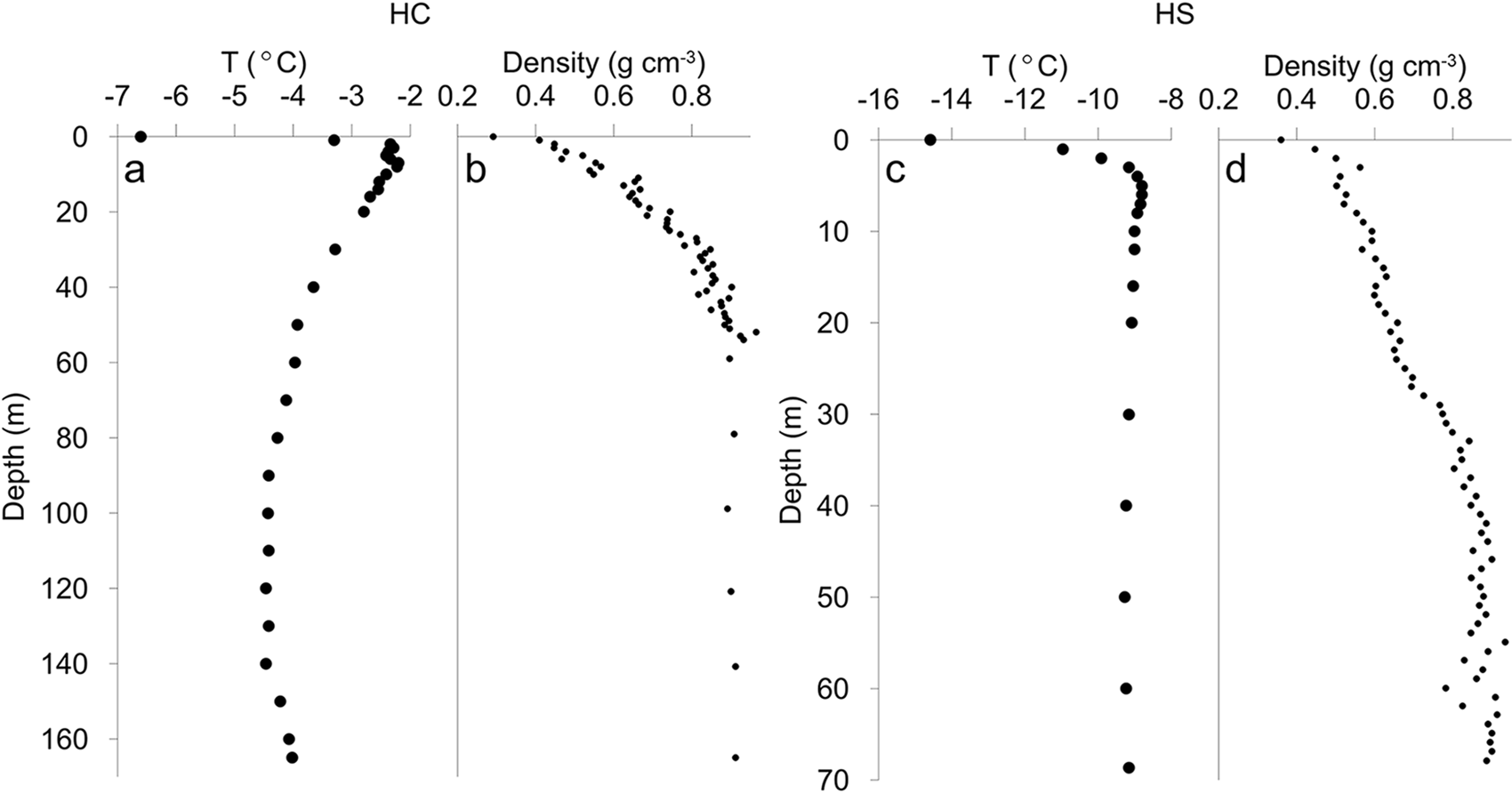
Figure 2. (a, c) Borehole temperature and (b, d) density profiles for HC and HS sites.
3.2. Ice thickness, bedrock topography and accumulation distribution
The 40 MHz GPR profiles at both sites reveal multiple continuous surface conformable reflectors within the upper 35–40 m (360–420 ns) (Figures 3 and 4). The internal reflections seen on radargrams caused by changes in the dielectric properties were attributed to density variations. The lower part of the radargrams did not show any strong reflections from the internal layers, which is indicative of the complete firn–ice transition and a uniform ice density distribution. The observed continuous reflectors in the upper part of radargrams are isochrones composed of a number of variable-density layers. Internal layers originate from surface accumulation and are subsequently altered by compaction and ice flow at greater depths.
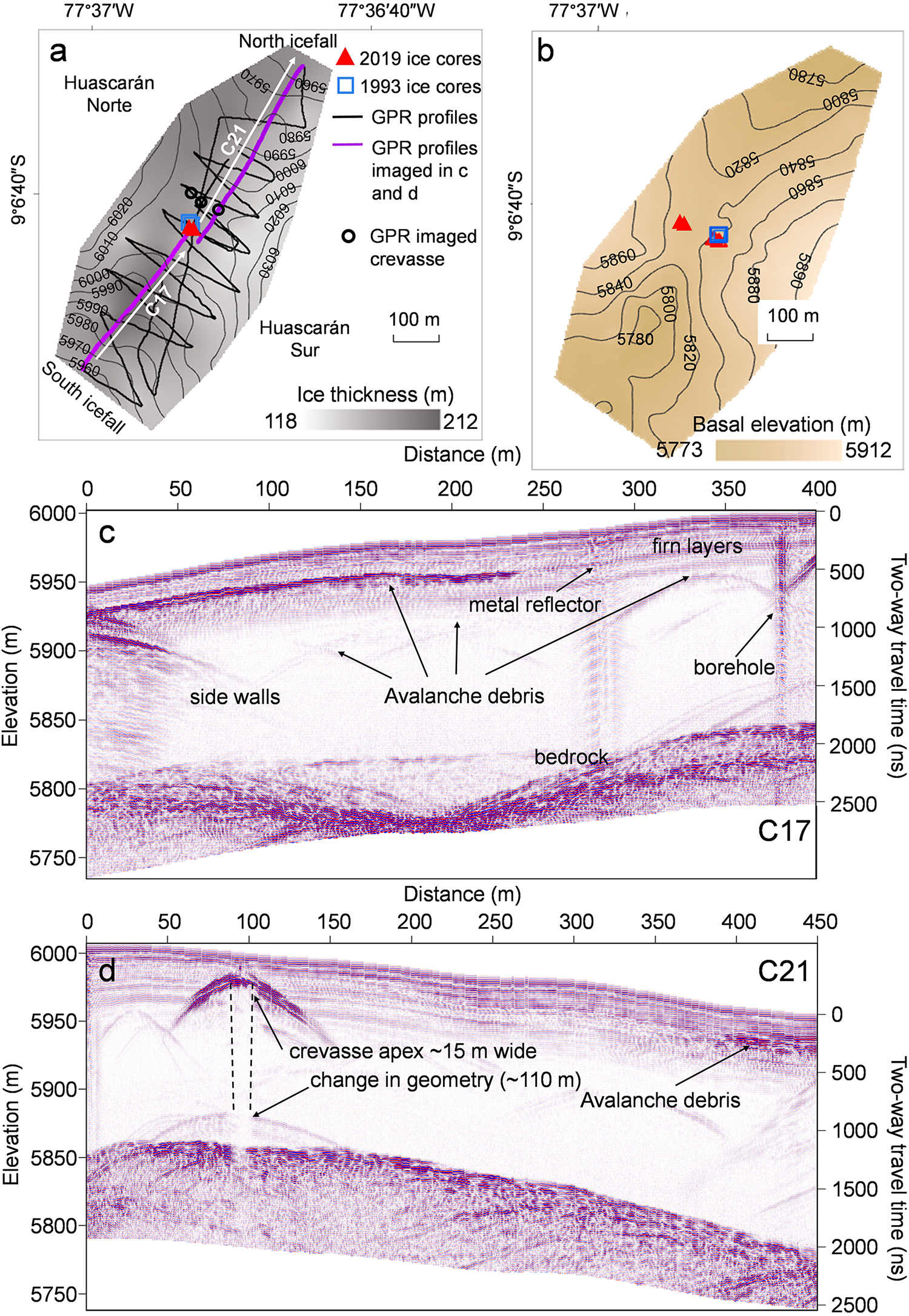
Figure 3. (a) Map showing the Huascarán col (HC) site surface elevation contours, drill sites location, GPR profiles including locations of 2 profiles imaged in c and d, crevasse location and ice thickness measured by GPR; (b) bedrock elevation at HC site; (c, d) 40 MHz profiles showing reflections from bedrock, side walls and multiple internal reflections from different sources.
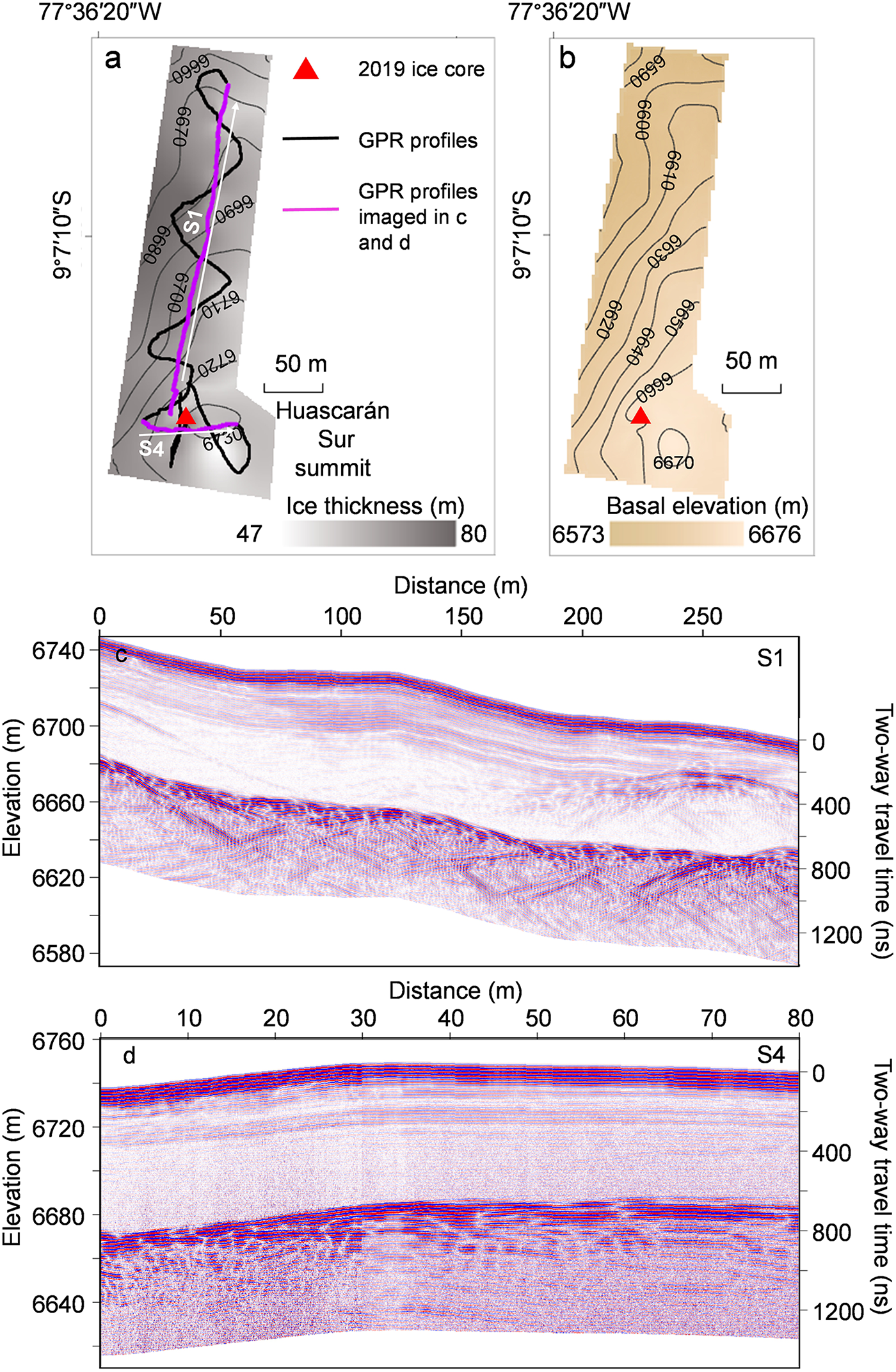
Figure 4. (a) Map showing Huascarán summit (HS) site surface elevation contours, drill site location, GPR profiles including locations of 2 profiles imaged in c, d and ice thickness measured by GPR; (b) bedrock elevation at HS site; (c, d) 40 MHz profile showing strong bedrock reflection and firn layers down to 40 m.
Strong bedrock reflections were detected on all 40 MHz radargrams. GPR measurements revealed the complex basal topography of the Huascarán col with the ice depth ranging from 117 to 212 m (Figure 3). Maximum depths are located 200 m southwest from the drill site where a 40–60 m depression in bedrock topography is seen, while ice depths are shallower towards both summit peaks. The ice divide is located in the middle of the col where the bedrock elevation is 5840 m asl and the average ice thickness is 170 m. The 2019 and 1993 drill sites are located close to the center of the ice divide above a slight bedrock slope of 10 degrees, which is a continuation of the Huascarán Sur peak slope. The GPR ice thickness measurements agree well with borehole depths at the 1993 and 2019 drill sites (Table 1). Available estimates on glacier surface elevation change (Seehaus and others, Reference Seehaus, Malz, Sommer, Lippl, Cochachin and Braun2019; Hugonnet, Reference Hugonnet2021) indicate only minor (∼0.15 ± 1.3 m a−1) positive elevation changes at the Huascarán col since 2000.
Table 1. Huascarán drill sites coordinates, borehole depths and GPR measured depths
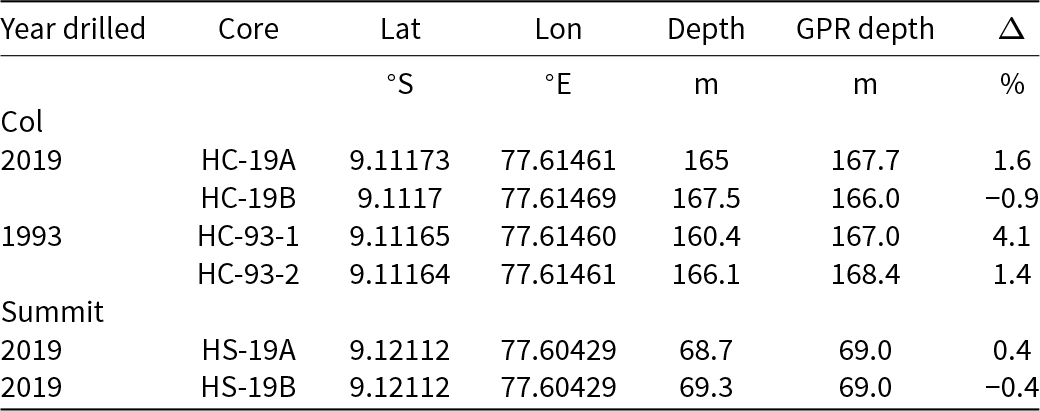
The surface and basal topography of the Huascarán Sur summit reveals a simple ice-dome-like structure. The average measured ice thickness for the HS site was 68 ± 4 m, with a maximum measured depth of 79 ± 4 m. The measured ice thickness near the drilling site was 69 ± 4 m, comparable to the borehole depth of 69.3 (HS-19A) and 68.7 and (HS-19B).
Side reflections are seen on radargrams from profiles perpendicular to the col center line as well as on profiles proximal to exposed crevasses close to the south icefall (Figure 3c). Side reflections occur because of the GPR profile’s close proximity to the valley headwall when GPR gets closer to the wall than to the bedrock or to sidewalls of open crevasses. Discrete random point reflections were also detected on a number of radargrams within the col. We interpret them as buried sporadic avalanche or ice fall debris (Campbell and others, Reference Campbell, Roy, Kreutz, Arcone, Osterberg and Koons2013). A layer of strong reflections was found on several radargrams close to the Huascarán Norte wall at the same depth (Figure 3c) which we interpret as avalanche debris. This layer is also consistent with the avalanche debris detected by 900 MHz radar (Figure 6c). It is unclear whether this layer is a result of one large avalanche or a series of avalanches which was later covered by accumulation. Other reflectors seen in the radargrams likely include a reflection from a piece of metal, as well as reflections from the electromechanical drill at the borehole (Figure 3b).
Snow pit and ice-core stratigraphy observations at the HC revealed multiple 1–3 cm ice lenses and ice layers mostly resulting in large density variations over short depth ranges which caused multiple reflections on high-frequency (900 MHz) radargrams (Figure 5a). The combination of the density, stratigraphy and isotopic composition profiles enabled the snow accumulation distribution to be estimated. The high amplitude isochrones at approximately 2.7 m (35 ns) depth around the drill site were attributed to the end of the 2018 dry season (Figures 5, 6).
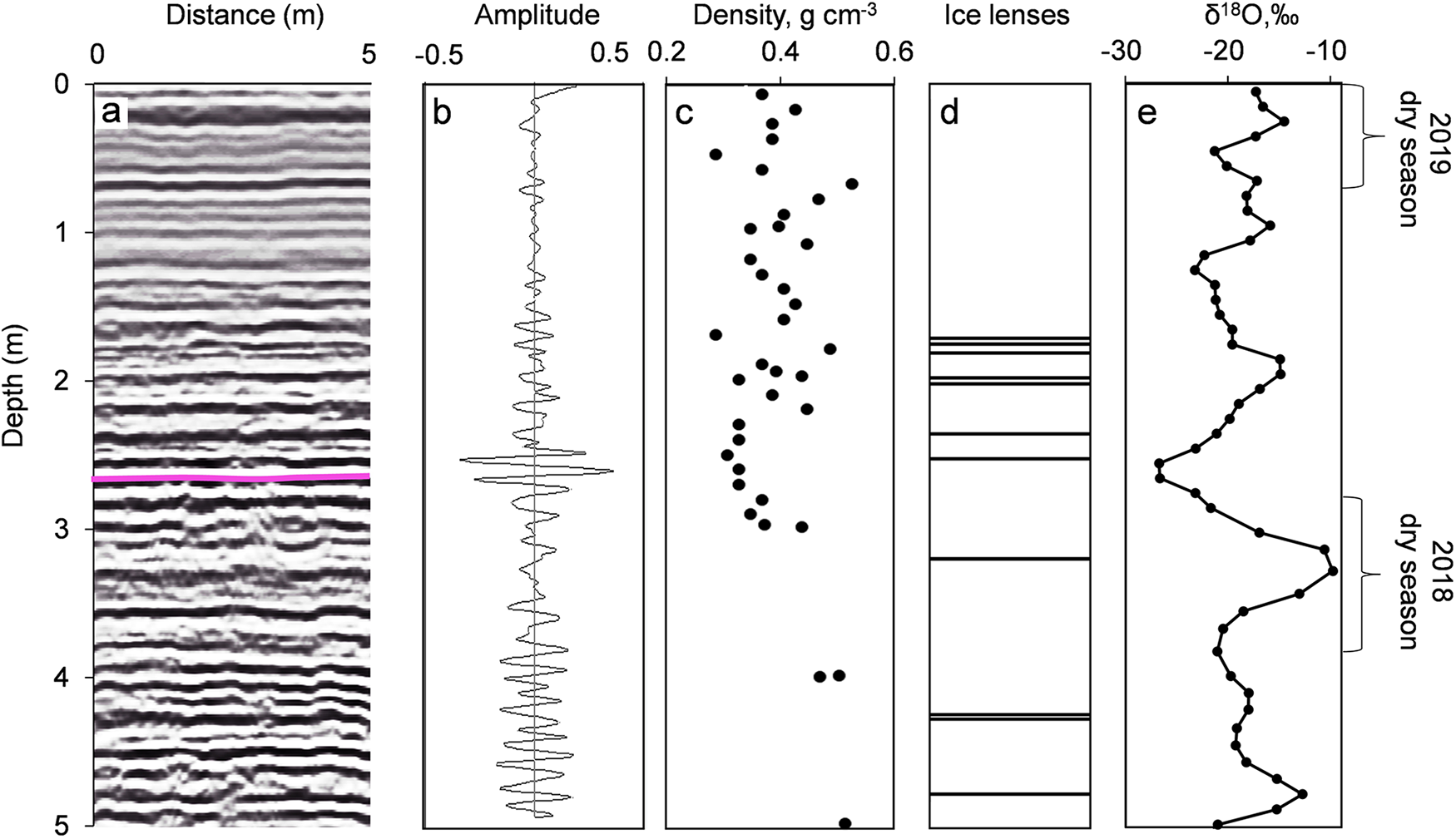
Figure 5. (a) A 900 MHz GPR radargram with annual layer (beginning of the 2019 accumulation) shown as a purple line; (b) GPR signal amplitude; (c) density; (d) stratigraphy and (e) isotopic composition at the HC 2019 drill site.
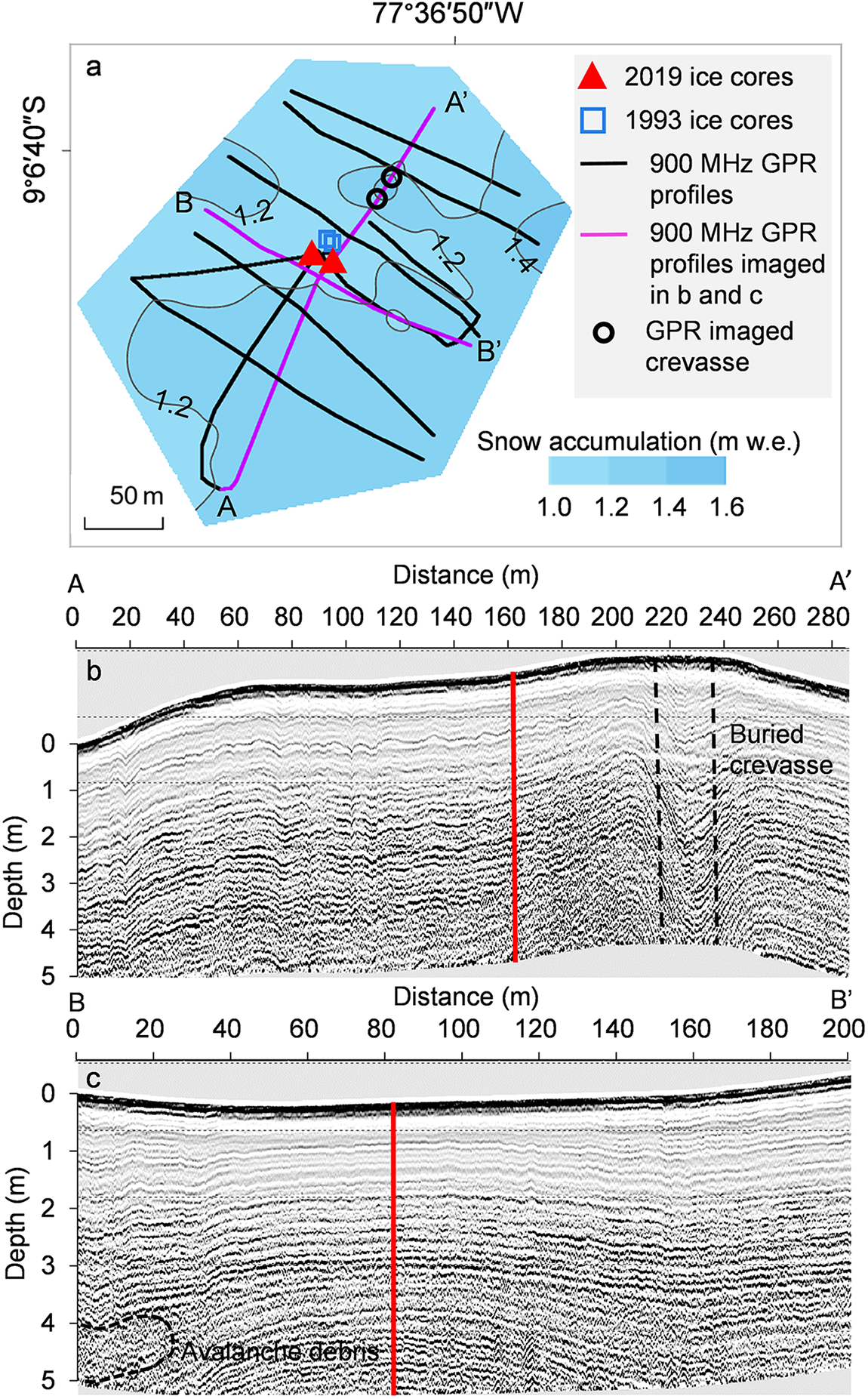
Figure 6. (a) Snow accumulation distribution, location of two selected 900 MHz GPR profiles, location of HC ice-core drill sites and detected crevasse; (b, c) topographically corrected GPR radargrams. The borehole location is shown as a thick red line. Note the dome-like shape of internal reflections at the ice divide (c). Avalanche debris and buried crevasse are shown as black dashed lines.
The 900 MHz GPR results show the uniform accumulation distribution and smooth, continuous, undisturbed dome-like internal glacier structure near the drilling site. A slight thickening of the stratigraphy and snow accumulation was observed towards both the north and south peak slopes and north and south ice cliffs with the minimum snow and firn layer thickness observed close to the drill site. 2018/2019 accumulation values range from 1.15 to 1.26 m.w.eq. at the ice divide. One of the 900 MHz profiles shows an area of interrupted stratigraphy at 4 m depth close to the Huascarán Norte summit slope (Figure 6c) likely due to avalanche debris. Avalanche debris was observed during the field season on both slopes of the col however, they do not reach the vicinity of the drill sites.
From the combined high- and low-frequency GPR profiles we identified a buried crevasse. It is located near the ice divide in a west-east direction perpendicular to the ice flow, 60 m to the north-east of the drill site. The 900 MHz profile collected from N to S across the divide reveals depressions in stratigraphy, which shows typical sagging snow bridges over a buried crevasse of ∼10–15 m width (Figure 6b). The same crevasse was also detected at three low frequency profiles seen as the hyperbolas at ∼15 m depth in Figure 3d. The crevasse narrows towards the north-east. From the GPR alone it is impossible to confirm the depth of the crevasse as the signal is strongly attenuated with depth by multiple reflections from the crevasse apex. Weak hyperbolas detected at the depth of ∼110 m indicate a change in the crevasse geometry and a possible closing. The crevasse is filled with snow and firn and was not visible at the surface.
GPR results show a complex internal structure of the glacier at the HC site. The conformable stratigraphy is observed throughout the col with avalanche debris detected closer to sidewalls and a buried crevasse close to the ice divide. We did not detect any reflections around the drill site which would indicate disrupted stratigraphy, indicating that a continuous stratigraphic record is preserved in the ice cores. Although we cannot rule out the possibility of small sporadic avalanches or ice fall debris reaching the vicinity of the drill site, this area is least influenced by such events compared to most of the col, including the observed depression in bedrock topography to the southwest of the ice divide where multiple avalanche debris reflections were detected at various depths.
3.3. Modeling results
Figure 7 provides an insight into both vertical and horizontal flow velocity components. Modeled velocities range from less than 1 ma−1 at the ice divide to up to 15 ma−1 near the icefall. These values align with typical ice flow velocities reported for cold-based, saddle-type glaciers (Campbell and others, Reference Campbell, Roy, Kreutz, Arcone, Osterberg and Koons2013; Licciulli, Reference Licciulli2018). Although ice-flow velocities have not been previously measured on Huascarán, global estimates suggest moderate ice flow velocities of up to 13 ma−1 at the HC drill site location (Figure 7b). This is unexpected, considering the flat surface topography and frozen bed conditions which are typically associated with reduced flow velocities. Overall, there is an agreement between Elmer/Ice model and remote sensing data in terms of ice flow directions; however, results from remote sensing show higher velocities by a factor of 3 on average within the model domain with a maximum of 34 ma−1 calculated for the areas close to northeast icefall. Given that the model domain is relatively small (∼350 × 850 m) with an average depth of 160 m, the current method requires calibration to realistically reproduce the flow over steep bedrock slopes and complex bedrock topography. The presented velocity field was obtained using an enhancement factor E = 0.01, which implies stiffer ice than expected for a temperature of −4°C. Using the suggested standard values for rate factor A, the model produces unrealistically high ice flow velocities as soon as the slope increases. Another major limitation of the current model setup is the assumptions made regarding boundary conditions, density profile, steady state, and constant temperature. Despite the simplifications, this approach produced a realistic velocity field and age distribution, both with depth and spatially.

Figure 7. Model results showing (a) modeled horizontal velocity for the solution with arrows showing orientation and colors representing magnitude; (b) horizontal velocity from Millan and others 2022; (c) three-dimensional mesh used to approximate the geometry of HC; (d) cross sections from A-A’ and B-B’ in (a) normal and parallel to the ice-divide axis showing modeled ice ages; (e) velocity cross section normal to the axis of the ice divide with arrows showing orientation. HC-19A borehole location is shown as a purple line.
The model tends to slightly underestimate accumulation in the vicinity of the drill site and accumulation closer to the Huascarán Sur slopes (Figure 8). The velocity field is only influenced by constant surface and bedrock topography and does not account for avalanche input or snow redistribution by wind. Both modeled and measured accumulation values indicate an area of uniformly low accumulation rate upstream of the drill sites.
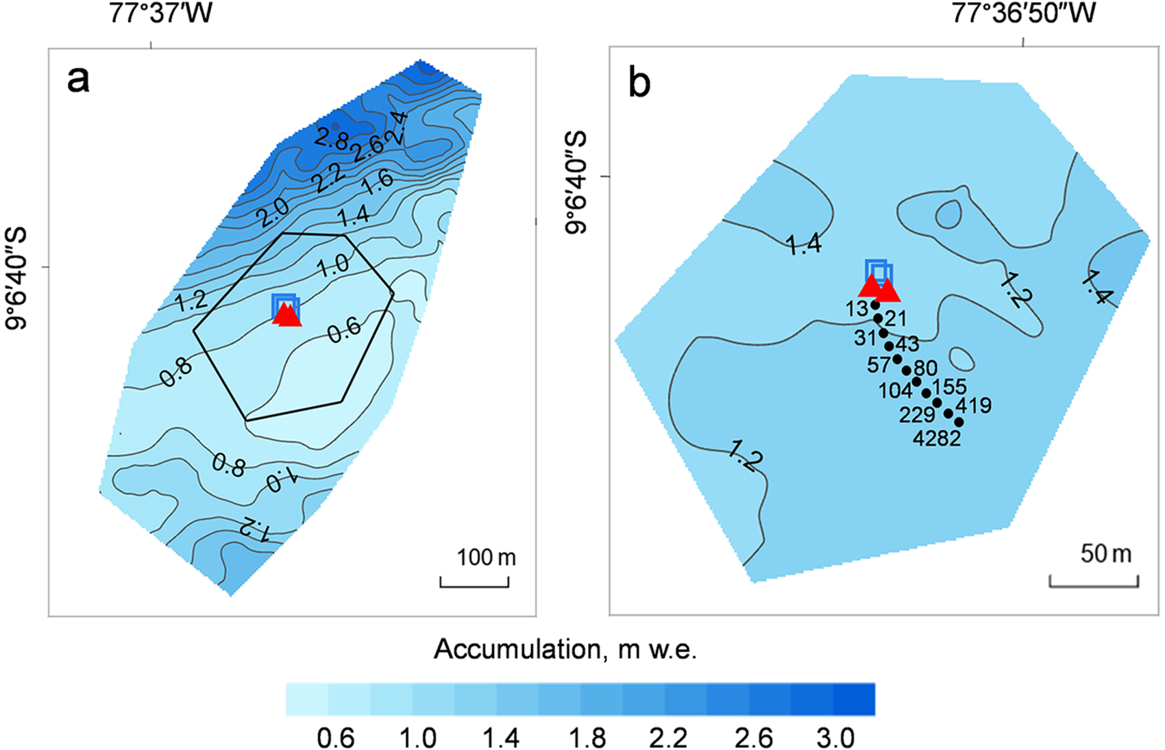
Figure 8. (a) Modeled accumulation distribution at the HC site, black polygon indicates position of figure b, 1993 (blue squares) and 2019 (red triangles) drill sites are shown; (b) measured accumulation distribution, source points calculated from backward trajectories for HC-19A drill site using the Runge–Kutta method (paraview) are indicated with black dots, the corresponding ages at the borehole location (in years) are shown.
The calculated ages of the HC glacier, derived from the Elmer/Ice model, generally aligns with the existing 1993–2019 ice-core chronology described above (Figure 9). However, the model tends to slightly overestimate ages at shallower depths by approximately 3 years, while underestimating the age closer to the basal ice.
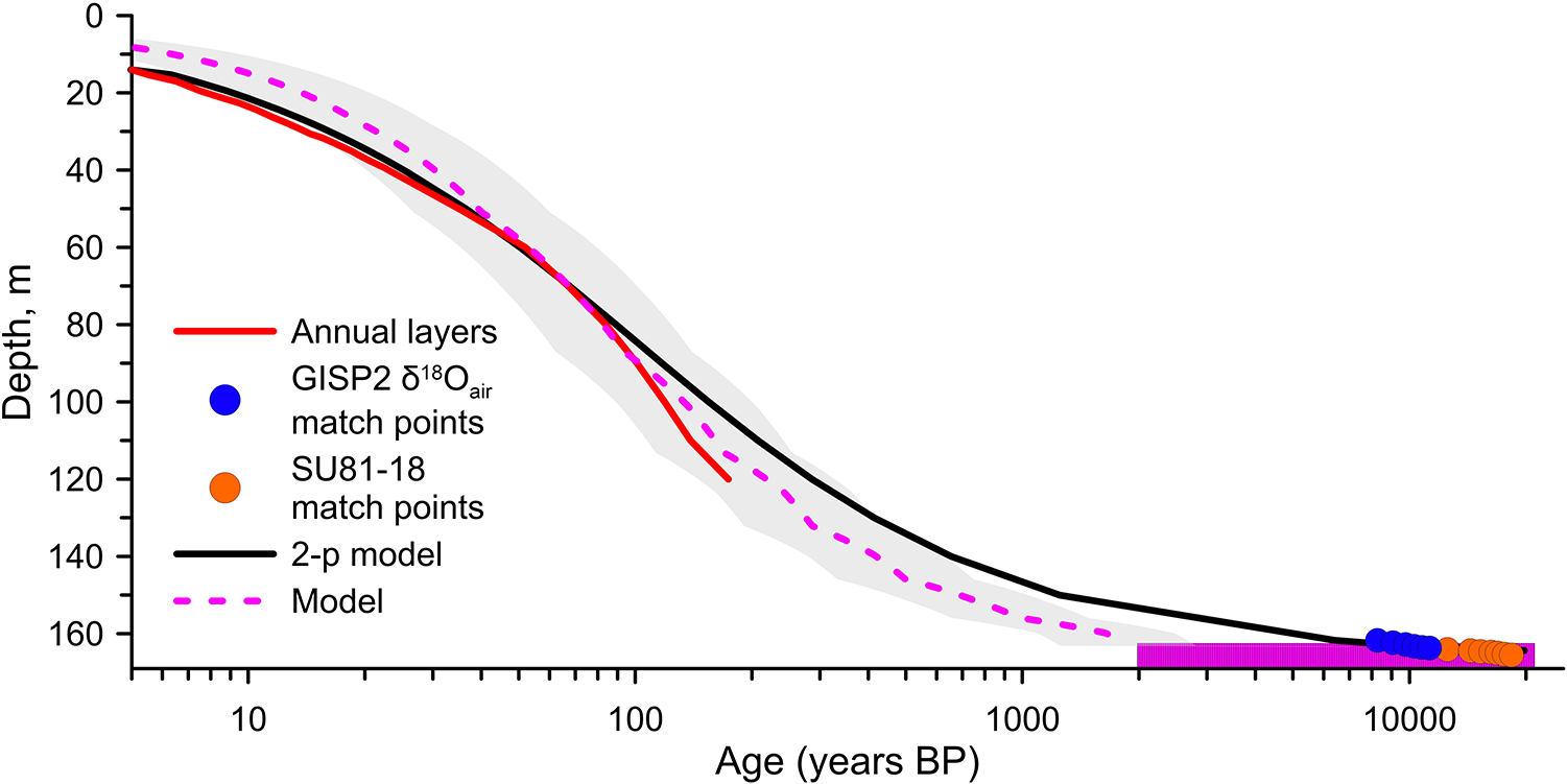
Figure 9. Timescale for Huascarán core composite of HC-93-2 and HC-2019-B. Modeled ice age calculated using the dating equation (Elmer/Ice, dashed purple line with the shaded area indicating the range of model outcomes considering an enhancement factor of ±50%). purple box depicts highly uncertain modeled basal ages. Annual layer counting was possible for the upper 125 m (red line). Matching between δ18oatm in the GISP2 ice core and the Huascarán ice (Davis and Thompson, Reference Davis and Thompson2006). The SU81-18 match points were derived from matching the δ18o from the lowest 3 m of the Huascarán core (i.e. the LGS) with the δ18o from a tropical north Atlantic marine core (Davis and Thompson, Reference Davis and Thompson2006). The 2p-model (Bolzan, Reference Bolzan1985) is depicted by the solid black line and is discussed in the text. Ages are expressed as years BP (with respect to the date of drilling).
Backward trajectories calculated for drill sites at HC show that layers 3–4 m above the bedrock were formed around 70–80 m south-east of the drill site. Therefore, we do not expect any significant upstream effect as the measured accumulation distribution is uniform.
4. Discussion
From 1991 to 1993, snow accumulation was measured using a network of 15 stakes on the HC. The 1991 to 1992 average annual snow accumulation obtained from the stakes was 1.3 m w.e., with values ranging from 1.13 to 1.25 m w.e. at the ice divide (Thompson, Reference Thompson1995). This is consistent with the 1960–2019 annual average accumulation of 1.4 m, i.e. estimated from the 2019 ice-core data (Weber, Reference Weber2023) as well as with the snow accumulation distribution determined from the high frequency radar measurements.
Short-pulse radar measurements were completed in 1993 at the same 15 points on the HC. The measured ice thickness ranged from 127 m to 218 m (Thompson, Reference Thompson1995). The direct comparison of these records is problematic due to potential positioning errors during the 1992–1993 field campaign and can only be considered as qualitative. Measurements made in 2019 confirm the previous estimates for the ice thickness of the HC. The point-by-point comparison shows that thickness distribution was in most cases interpreted correctly in 1993 and the correlation (r 2) for 13 points is 0.73 (5%, std = 7%) with slightly larger ice thicknesses measured in 1993 within the uncertainty estimates (Fig. S1). Two points measured on the southern part of the col in 1993 showed 30% higher ice thicknesses than measured in 2019; this is likely due either to positioning errors or misinterpretation of the sidewall reflections at these two locations when interpreting point radar measurements in 1993.
The crevasse at HC was detected near the ice divide. Modeling results suggest quasi-stagnant ice at the ice divide with slowly increasing surface ice flow in north-east direction. The modeled ice flow velocity field reproduces the direction of the crevasse, with the center of the crevasse coinciding with the ∼5 ma−1 velocity isoline. Campbell and others, (Reference Campbell, Roy, Kreutz, Arcone, Osterberg and Koons2013) reported several buried crevasses they identified using GPR measurements at and near the ice divide on Mount Hunter (Alaska Range, USA). One of the crevasses was detected in GPR radargrams beginning at 50 m depth, suggesting that it formed at depth (Campbell and others, Reference Campbell, Roy, Kreutz, Arcone, Osterberg and Koons2013). Although it was shown previously that under certain conditions crevasse formation can occur at depths of 15 to 30 m (Nath and Vaughan, Reference Nath and Vaughan2003), there is still a lack of direct evidence of such a process (Colgan, Reference Colgan2016). We detected the crevasse apex at 15 m depth overlaid with sagging snow bridges with the depth of the crevasse potentially exceeding 100 m. Our data can neither confirm nor reject the hypothesis of the crevasse formation at depth. This site may potentially be used for future research on crevasse formation and dynamics at ice divides. Since according to GPR measurements the borehole is located 60 m away from this crevasse, these results show the importance of conducting GPR surveys at drill sites.
Direct comparison of the ice thickness measured using GPR and available modeling results (Farinotti, Reference Farinotti2019; Millan and others, Reference Millan, Mouginot, Rabatel and Morlighem2022) reveal large discrepancies for the HC and HS sites (Fig. S2). Both models underestimate ice thickness. The average measured ice thickness for the HS col area is 160.2 m (std = 20.1 m) while Farinotti (Reference Farinotti2019) data suggest an average ice thickness of 78.1 m (std = 16.4 m) and Millan and others, (Reference Millan, Mouginot, Rabatel and Morlighem2022) estimated an even shallower ice thickness of just 57.0 m (std = 16.4 m). Similarly, the ice thickness at the drill site (165-167.5 m) is 93.1 m according to Farinotti (Reference Farinotti2019) and just 55.3 m according to Millan and others, (Reference Millan, Mouginot, Rabatel and Morlighem2022). At the HS both datasets also show shallower ice than measured. Average modeled ice thickness for the HS site is 35.0 m (std = 4.2 m) and 28.8 (std = 12.8 m) as reported by Farinotti (Reference Farinotti2019) and Millan and others, (Reference Millan, Mouginot, Rabatel and Morlighem2022), respectively. The average ice thickness measured using the GPR at the HS site is 68 m (std = 4 m). Both HC and HS sites are in the ice divide areas. The model of Farinotti (Reference Farinotti2019) is known for producing larger uncertainties in ice-cap-like areas, as calculations of ice thicknesses along the flowlines result in underestimation of ice thickness close to boundaries between RGI60 glacier outlines. It was shown that these two models tend to underestimate ice thickness for ice caps in Scandinavia (Frank and Van Pelt, Reference Frank and Van Pelt2024). Our results highlight the existing large uncertainties of the available ice thickness models, especially for accumulation areas close to ice divides. Therefore, these data should be used with caution for applications that require knowledge of ice thickness and bedrock topography (e.g. selection of ice-core drilling sites, depth age modeling, estimation of water storage). The direct accumulation-zone measurements described in this research can be used to improve the accuracy and reliability of future modeling efforts.
The lack of direct ice flow measurements prevents the validation of modeling results against ground truth data. However, the ice velocity field generated by the model setup closely aligns with the measured depth-age distribution at the drill site. It is likely that the ice velocity values derived from remote sensing (Millan and others, Reference Millan, Mouginot, Rabatel and Morlighem2022) are overestimated. This overestimation may be attributed to weak signals in flat accumulation areas, low spatial resolution, and interpolation between fast-flowing icefall regions on Huascarán’s slopes, which in turn leads to an underestimation of ice thickness. The modeled age of the ice at 3 m above the bedrock is estimated at ∼4700 years, supporting the hypothesis that a Holocene record is preserved at this site. The lowest few meters can contain thousands of years due to significant thinning near the bedrock, so that age models are highly uncertain close to the bottom. The model does not account for temporal variations in accumulation, which adds to the overall uncertainty.
5. Conclusions
The 2019 expedition to Nevado Huascarán provided valuable glaciological and geophysical data, including the results of analyses of four ice cores drilled to bedrock at the col and summit. Analysis of borehole temperature profiles confirmed the frozen condition of the ice at the col, while revealing colder conditions at the summit. The measured ice thicknesses ranged from 117 to 212 m at the Huascarán col, with an average thickness of 170 m, and from 68 to 79 m at the summit. The comprehensive GPR survey conducted during the expedition enabled detailed mapping of the ice thickness distribution and basal topography. The presence of buried crevasses, avalanche debris, and variable-density layers shows the complexity of the glacier’s internal structure. A 3D full-Stokes glacier model confirms the choice of the optimal drill site location. Comparison with existing global modeling data revealed significant discrepancies in ice thickness estimates for the Huascarán col and summit with measured ice thicknesses exceeding those predicted by models. Overall, the results from the 2019 expedition underscore the importance of field observations for model validation and calibration.
Supplementary material
The supplementary material for this article can be found at https://doi.org/10.1017/jog.2025.20.
Data availability statement
Ice thickness data are archived at https://www.ncei.noaa.gov/access/paleo-search/study/41000.
Acknowledgements
Funding for the 2019 drilling project on Huascarán was provided by the National Science Foundation (NSF) Paleoclimate Program award AGS 1805819 and by The Ohio State University (OSU). We acknowledge the efforts of the OSU Byrd Polar and Climate Center’s research team. Dr. Ping-Nan Lin and Donald Kenny (OSU-BPCRC) performed the analyses of the Huascarán ice cores for stable isotopes, dust, and major ion chemistry.
We acknowledge leaders and residents of local communities who allowed us access to the mountain at the end of the field season to retrieve the ice cores and equipment. We acknowledge the efforts of the Félix Benjamin Vicencio and 38 mountaineers and porters. We acknowledge the assistance of Martín Vizcarra Cornejo, former President of Peru; Lucía Ruiz Ostoic, Minister of the Environment; Abog Víctor Saavedra Espinoza, General Manager of INAIGEM; Gisella Orjeda Fernández, former Executive President of INAIGEM; Willian Martínez Finquin, Director of Huascarán National Park; and engineers César Portocarrero Rodríguez, William Tamayo Alegre, and Gustavo Valdivia Corrales. We thank Father Alessio Busanto and all the volunteers at the Alpine Hut for their assistance.
This is Byrd Polar and Climate Research Center contribution number C-1635.
Author contributions
S.K. conceived the study, led data analysis and drafted the manuscript. L.G.T contributed to the conceptualizing and writing of the paper and was a principal investigator. J.F.B provided feedback and also contributed to writing. I.L. contributed to fieldwork and interpretation of GPR data. G.Ch. conducted modeling. F.Sh contributed to fieldwork. All authors discussed results, implications, provided feedback and approved of the final manuscript.
Competing interests
The authors declare none.
Appendix A—Ice Flow Model
The calculation of the velocity field was performed on the basis of a 3D stationary full Stokes model with a rheological law for a compressible nonlinear viscous medium (ice/firn) (Gagliardini and Meyssonnier, Reference Gagliardini and Meyssonnier1997). We have applied a purely mechanical (isothermal) flow model. Information on the quantities used in the mathematical model is given in Table A1. The units in the table are chosen to be more representative, rather than coherent.
Table A1. Physical parameters used for the simulations with Elmer/Ice
A.1. Dating problem
In order to obtain a 3D age field of ice/firn  $\mathcal{A}$(x, y, z), we first calculated the velocity field ${\boldsymbol{v}}$(x, y, z) in the computational domain and then solved the dating equation d $\mathcal{A}$/dt = 1, or
 \begin{equation}\frac{{\partial \mathcal{A}}}{{\partial t}} + {\boldsymbol{v}} \cdot {\text{grad}}\mathcal{A} = 1\end{equation}
with a boundary condition of zero age at the surface of the glacier:
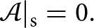 \begin{equation}\mathcal{A}{|_{\text{s}}} = 0.\end{equation}
 Due to the steady-state assumption ∂  $\mathcal{A}$/∂t ≡ 0.
A.2. Constitutive equations
The constitutive equations of the model are subsequently introduced. Based on the surface heights, a depth field is calculated in the entire 3D domain:
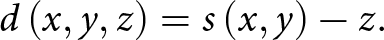 \begin{equation}d\left( {x,y,z} \right) = s\left( {x,y} \right) - z.\end{equation}
On the basis of density distribution in the HC-19A ice core, the ice/firn density in the glacier is represented as a function of depth as follows:
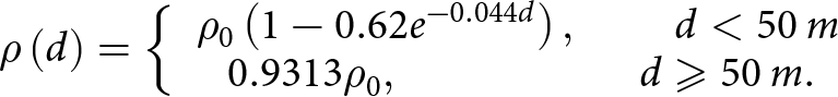 \begin{equation}\rho \left( d \right) = \left\{ {\begin{array}{*{20}{c}}
{{\rho _0}\left( {1 - 0.62{e^{ - 0.044d}}} \right),\,\,\,\,\,\,\,\,\,\,\,\,\,d \lt 50\,m\,} \\
{0.9313{\rho _0},\,\,\,\,\,\,\,\,\,\,\,\,\,\,\,\,\,\,\,\,\,\,\,\,\,\,\,\,\,\,\,\,\,d \geqslant 50\,m.}
\end{array}} \right.\end{equation}
\begin{equation}\rho \left( d \right) = \left\{ {\begin{array}{*{20}{c}}
{{\rho _0}\left( {1 - 0.62{e^{ - 0.044d}}} \right),\,\,\,\,\,\,\,\,\,\,\,\,\,d \lt 50\,m\,} \\
{0.9313{\rho _0},\,\,\,\,\,\,\,\,\,\,\,\,\,\,\,\,\,\,\,\,\,\,\,\,\,\,\,\,\,\,\,\,\,d \geqslant 50\,m.}
\end{array}} \right.\end{equation}Thus, according to Eqn (A4) the density value increases up to 900 kg m–3 in the upper 50 m layer and maintains this constant value at greater depths. A similar approximation obtained from the ice core HC-19B differs from (A4) by less than 26 kg m–3 at any depth.
The functions of the relative density φ (φ =  $\rho /{\rho _0}$)
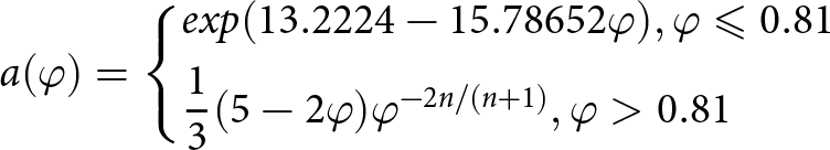 \begin{equation}a(\varphi ) = \left\{ \begin{gathered}
exp(13.2224 - 15.78652\varphi ),\varphi \leqslant 0.81 \hfill \\
\frac{1}{3}(5 - 2\varphi ){\varphi ^{ - 2n/(n + 1)}},\varphi \gt 0.81 \hfill \\
\end{gathered} \right.\end{equation}
\begin{equation}a(\varphi ) = \left\{ \begin{gathered}
exp(13.2224 - 15.78652\varphi ),\varphi \leqslant 0.81 \hfill \\
\frac{1}{3}(5 - 2\varphi ){\varphi ^{ - 2n/(n + 1)}},\varphi \gt 0.81 \hfill \\
\end{gathered} \right.\end{equation}and
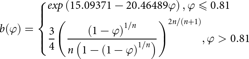 \begin{equation}b(\varphi ) = \left\{ \begin{gathered}
exp\left( {15.09371 - 20.46489\varphi } \right),\varphi \leqslant 0.81 \hfill \\
\frac{3}{4}{\left( {\frac{{{{(1 - \varphi )}^{1/n}}}}{{n\left( {1 - {{\left( {1 - \varphi } \right)}^{1/n}}} \right)}}} \right)^{2n/(n + 1)}},\varphi \gt 0.81 \hfill \\
\end{gathered} \right.\end{equation}
\begin{equation}b(\varphi ) = \left\{ \begin{gathered}
exp\left( {15.09371 - 20.46489\varphi } \right),\varphi \leqslant 0.81 \hfill \\
\frac{3}{4}{\left( {\frac{{{{(1 - \varphi )}^{1/n}}}}{{n\left( {1 - {{\left( {1 - \varphi } \right)}^{1/n}}} \right)}}} \right)^{2n/(n + 1)}},\varphi \gt 0.81 \hfill \\
\end{gathered} \right.\end{equation}are used to construct the flow law relations in accordance with (Gagliardini and Meyssonnier, Reference Gagliardini and Meyssonnier1997).
The strain-rate tensor is a symmetric part of the velocity gradient:
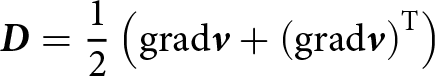 \begin{equation}{\boldsymbol{D}} = \frac{1}{2}\left( {{\text{grad}}{\boldsymbol{v}} + {{\left( {{\text{grad}}{\boldsymbol{v}}} \right)}^{\text{T}}}} \right)\end{equation}
Decomposing the strain-rate tensor into an isotropic and a deviatoric parts, we obtain:
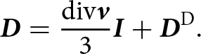 \begin{equation}{\boldsymbol{D}} = \frac{{{\text{div}}{\boldsymbol{v}}}}{3}{\boldsymbol{I}} + {{\boldsymbol{D}}^{\text{D}}}.\end{equation}
Hereinafter the superscripts T and D denote the transpose and the deviator of a tensor, respectively; I is the unit tensor. The first invariant of the strain-rate tensor is represented in the form of the velocity divergence.
Following (Gagliardini and Meyssonnier, Reference Gagliardini and Meyssonnier1997), we introduce the tensor invariant
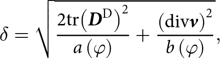 \begin{equation}\delta = \sqrt {\frac{{2{\text{tr}}{{\left( {{{\boldsymbol{D}}^{\text{D}}}} \right)}^2}}}{{a\left( \varphi \right)}} + \frac{{{{\left( {{\text{div}}{\boldsymbol{v}}} \right)}^2}}}{{b\left( \varphi \right)}}} ,\end{equation}
where tr denotes the trace of a tensor. Then the viscosity of ice/firn can be expressed as follows:
 \begin{equation}\mu \left( {\delta ,\,\varphi } \right) = \frac{{{{\left( {2EA{\delta ^{n - 1}}} \right)}^{ - 1/n}}}}{{a\left( \varphi \right)}}.\end{equation}
The constant flow enhancement factor E in Eqn (A10) is used as a calibration parameter.
After splitting Cauchy stress tensor into an isotropic and a deviatoric part
 \begin{equation}{\boldsymbol{\sigma }} = - p{\boldsymbol{I}} + {{\boldsymbol{\sigma }}^{\text{D}}}\end{equation}
we can write the rheological law in general form:
 \begin{equation}{{\boldsymbol{\sigma }}^{\text{D}}} = 2\mu {{\boldsymbol{D}}^{\text{D}}}.\end{equation}
A.3. Field equations
The field equations of the model are the volume balance equation
 \begin{equation}{\text{div}}\,\,{\boldsymbol{v}} + \frac{{b\left( \varphi \right)}}{{a\left( \varphi \right)\mu }}p = 0\end{equation}
and the Stokes equation
 \begin{equation}{\text{div}}\,\,{\boldsymbol{\sigma }} + \rho {\boldsymbol{g}} = 0.\end{equation}
A.4. Boundary conditions
Boundary conditions (BCs) are specified separately at three areas of the boundary of the computational domain: the surface, the base, and the lateral side.
A.4.1. Surface boundary condition
Surface BC apply to the part of the glacier surface under consideration (designated by the subscript s). The surface BC is the stress-free condition
 \begin{equation}{\left. {\left( {{\boldsymbol{\sigma }} \cdot {\boldsymbol{n}}} \right)} \right|_{\text{s}}} = 0.\end{equation}
A.4.2. Basal boundary condition
Basal BC (denoted by b) apply to the bedrock of the glacier. The basal BC implies a cold base (zero tangential velocity) and a small normal outflow ice velocity at the bedrock:
 \begin{equation}{\boldsymbol{v}}{|_{\text{b}}} = {v_{\text{b}}}{\boldsymbol{n}}{|_{\text{b}}}.\end{equation}
A.4.3. Lateral boundary conditions
Lateral BCs (denotation l) are specified at the vertical surface surrounding the modeled area and connecting the upper and lower parts of the computational domain boundary (glacier surface and bedrock). The lateral BCs are different for the north–south (l, NS) and east–west (l, EW) sides of the domain, since the outflow is applied only at the north and south icefalls (Figure 3a).
At the icefalls the stress-free condition is applied:
 \begin{equation}{\left. {\left( {{\boldsymbol{\sigma }} \cdot {\boldsymbol{n}}} \right)} \right|_{{\text{l}},{\text{ NS}}}} = 0.\end{equation}
At the sides where the slopes of Huascarán summits are located the normal velocity is set to zero, while tangential velocities are not constrained:
 \begin{equation}{\left. {\left( {{\boldsymbol{v}} \cdot {\boldsymbol{n}}} \right)} \right|_{{\text{l}},{\text{ EW}}}} = 0.\end{equation}
 The differential equations of Section A.3 together with the material equations of Section A.2 and the boundary conditions of Section A.4 form a complete boundary value problem for determining the unknown fields  ${\boldsymbol{v}}$ and p.


 Open access