Modeling Hierarchical Spatial Interdependence for Limited Dependent Variables

Abstract

Multilevel modeling accounts for outcome dependence across lower-level units due to unobserved group effects, while spatial modeling accounts for outcome dependence across units in the same level of analysis due to diffusion. Outcome dependence can occur simultaneously due to both spatial diffusion in the lower-level units and spatial diffusion in the unobserved group effects. For example, counties are nested within states and diffusion processes might take place at both levels of analysis. Building on recent research from the spatial econometrics and multilevel modeling literature, we propose a class of spatial hierarchical models with binary outcomes. One method accounts for spatially independent, unobserved group effects and the other method accounts for spatially dependent unobserved group effects. We propose a Bayesian approach to estimate such effects while also accounting for lower-level diffusion in the outcome, and provide software to estimate these models. Our Monte Carlo results demonstrate that failing to correctly account for diffusion and/or the nested structure of data can lead to bias in both parameter estimates and substantive effects. We apply these models to analyze the causes of civil rights protests in the United States in the 1960s.

1 Introduction

Theories about diffusion in political science are vast. These theories include diffusion of policy across states, conflict across countries, and defense policy across nations (Polo 2020; Sandler and Shimizu 2014; Simmons and Elkins 2004). The introduction and advancement of spatial regression models in political science have empowered researchers to appropriately model such spatial processes. Failing to accurately model spatial processes results in inefficiency at best and bias, inconsistency, and inefficiency at worst. The introduction of spatial regression models also introduced a new dimension to substantive interpretation. Scholars could now analyze how a change in an independent variable affects the dependent variable in the same unit (direct effect), the dependent variable in other units (indirect effects), and the total effect in all units due to a change in that independent variable (total effects).

Analyzing multilevel data is also popular in political science. These data are structured in a manner such that lower-level or level-1 units are nested in higher-level or level-2 units.¹ Two examples of data that contain a nested structure include units (level-2) that are each observed across multiple time periods (level-1) (e.g., time-series-cross-section data), and units at different levels of analysis (e.g., voters [level-1] in a county [level-2]). Due to the hierarchical nature of the data, estimating models that fail to account for the nested structure of these data lead to inaccurate inferences. This is because both level-1 and level-2 units can have their own effects. One such effect includes level-2 intercepts that account for unobserved effects that are invariant across level-1 units within each level-2 unit (fixed/random intercepts). At best, failing to account for the multilevel nature of data will result in inefficiency, and at worst, there will be bias, inconsistency, and inefficiency.

A budding vein of research now combines advances in spatial econometrics and hierarchical modeling to model diffusion at multiple levels of analysis (Dong and Harris 2015). Spatial models can account for outcome dependence across units in the same level of analysis due to diffusion and multilevel models account for outcome dependence across level-1 units due to unobserved group effects. However, there also exists the possibility that outcome dependence is a consequence of two processes occurring simultaneously. One such process is due to diffusion among level-1 units and the other process can be due to the presence of spatially dependent/independent level-2 unobserved group effects. Consider the civil rights protests in the United States in the 1960s. A level-1 diffusion process is when a county was more likely to experience a civil rights protest if nearby counties experienced civil rights protests due to the spread of information about protests through local news media (Andrews and Biggs 2006). As an example of spatially dependent level-2 effects, consider that the baseline propensities (unobserved state-level effects) for civil rights protests to occur in one state could have affected the baseline propensities for civil rights protests to occur in other states possibly due to interstate travel by civil rights activists (Andrews and Biggs 2006). As an example of spatially independent level-2 effects, consider that, hypothetically, interstate travel during that time was prohibited for all individuals; each state could have had its own baseline propensities that were independent of other states’ baseline propensities. Dong and Harris (2015) only account for level-1 and level-2 diffusion processes in their model and do not introduce a model that accounts for spatially independent level-2 unobserved group effects. Thus, estimating a model similar to theirs can lead to efficiency losses when there exist spatially independent level-2 unobserved group effects.

We introduce two hierarchical spatial strategies for binary outcomes. Our first proposed model, spatial autoregressive probit with random effects (SAR-RE), accounts for level-1 spatial diffusion in the outcome and only spatially independent, unobserved level-2 effects. Our second proposed model, hierarchical spatial autoregressive (HSAR) probit, accounts for diffusion at both level-1 and level-2 units and allows researchers to explicitly theorize about and test for the existence of multilevel diffusion processes.² We reach two main conclusions from a series of Monte Carlo experiments. First, as expected, estimating a spatial autoregressive (SAR) probit model or a SAR random effects probit model that only accounts for level-1 diffusion results in inaccurate inferences when there is also level-2 diffusion; the HSAR model performs well in this scenario. Second, we find that estimating an HSAR model results in accurate inferences when there is no spatial diffusion at either level and/or in the presence of non-spatial random effects. However, this comes with a cost of reduced precision because of the inefficiency from estimating extra parameters. We thus recommend that researchers at a minimum consider testing for higher-level spatial diffusion and then, based on these results, decide between the HSAR or a model it encompasses, e.g., SAR-RE.

2 The Importance of Spatial Probit Models

Many processes in political science have outcomes that are binary and are also affected by outcomes in other units. These include studies of territorial claims (Lee 2024), military regimes (Caruso, Pontarollo, and Ricciuti 2020), terrorism (Polo 2020), conflict (Lane 2016), and mediation (Böhmelt 2015). Spatial probit models allow researchers to test theories about such diffusion processes with binary outcomes. The spatial probit model can be written as

$$ \begin{align*} \boldsymbol{y^*} = \rho \boldsymbol{Wy^*} + \boldsymbol{X}\boldsymbol{\beta} + \boldsymbol{\epsilon}, \notag \end{align*} $$

where $\boldsymbol {y^*}$ is an $N \times 1$ vector of latent outcomes in all N units ( $y_i = 1 \text { if } y_i^*> 1$ and $y_i = 0$ otherwise), $\rho $ is the SAR coefficient, $\boldsymbol {X}$ is a matrix of predictors with dimensions $N \times K$ , $\boldsymbol {\beta }$ is a $K \times 1$ vector, and $\boldsymbol {W}$ is an $N \times N$ spatial weights matrix. In general, an important motivation for modeling spatial processes is that level-1 observations are not independent from each other, and thus, researchers need to appropriately calculate and interpret how a change in a predictor affects the outcome of interest. Failing to appropriately account for a spatial process can lead to an inefficient, biased, and inconsistent estimator. Similar to SAR models with continuous outcomes, researchers can calculate post-estimation substantive effects (direct, indirect, and total effects) of a change in a predictor using a spatial probit model. The direct effect measures the change in the propensity of an event occurring due to a change in a predictor in the same unit, the indirect effect measures the change in the propensity of an event occurring in other units due to a change in the propensity of an event occurring in the same unit as a result of a change in a predictor in that unit, and the total effect is the sum of the direct and indirect effects and measures the total change in the propensity of an event occurring due to a change in the predictor (e.g., Franzese, Hays, and Cook 2016; LeSage and Pace 2009).

3 The Importance of Modeling Unobserved Random Effects in Multilevel Data with Binary Outcomes

The motivation behind multilevel models is also non-independent observations. However, in this case, the level-1 observations (e.g., students) within a level-2 group (e.g., school) are not independent and the observations across level-2 groups are traditionally assumed to be independent.³ One commonly used model is the random intercepts probit model in which level-2 (j) intercepts affect the level-1 (i) outcome:

$$ \begin{align*} \text{Pr}(y_{ij}=1|x_{i}) = \Phi(\alpha_j + \beta x_i), \end{align*} $$

where $y_{ij}$ is a binary outcome, $\alpha _j$ is the level-2 intercept such that $\alpha _j \sim N(0, \sigma _\alpha ^2)$ , and $x_i$ is a level-1 predictor. The random intercepts model relies on the assumption that the predictor(s) and random intercepts are uncorrelated. Failing to account for random intercepts in the model leads to observed attenuation in $\beta _1$ in models with binary outcomes due to incorrect normalization (Cramer 2003; Neuhaus and Jewell 1993). As the residual variance increases, the normalized coefficient estimate decreases as the change in the residual variance unaccounted for affects the scaling of the coefficients (Cramer 2003, 81).

4 Multilevel Data and Multiple Diffusion Processes

For the most part, hierarchical models and spatial econometrics have developed as two distinct fields.⁴ The focus of the spatial econometrics literature is to explicitly model theoretically interesting diffusion processes. For example, Simmons and Elkins (2004) examine how liberal economic policies have diffused across countries over time. The hierarchical modeling literature implicitly assumes that units in a common group share some similar characteristics. The typical example often used is that students in the same classroom may often have correlated errors because they have the same teacher and share similar experiences within the classroom. Hierarchical models explicitly deal with this by accounting for the multilevel data structure in which lower-level units are nested within higher-level units.

There have been recent advances in the spatial econometrics literature that focus on combining multilevel and spatial modeling. For example, Dong and Harris (2015) proposed an HSAR model with which they estimated the effects of various factors on the leasing price of land parcels in China, where land parcels are grouped into various districts. Advances in spatial and hierarchical modeling combined with data availability have created opportunities to improve our understanding of politics. For example, while Mazumder (2018) investigates the persistent effects of civil rights protests on political attitudes, researchers may also want to investigate the conditions under which protests are likely to occur in some counties, but not in others. In addition to the diffusion of civil rights protests across counties because of the spread of information (Andrews and Biggs 2006), two other features are worth considering. First, counties are nested within states. Different states might have had different political, social, and economic conditions that could have affected the common baseline propensity of civil rights protests to occur in counties within the same state. Second, the baseline propensity for civil rights protests could have diffused across states.

Our proposed model takes into account the nested structure of data and also tests for the existence of a diffusion process among higher-level units. If a scholar has a theory about how a certain predictor of interest affects the diffusion of civil rights protests and does not account for the multilevel structure of the data by modeling diffusion at both level-1 (across counties within states) and level-2 (across states) units, they may erroneously conclude that predictor has a larger-than-true indirect effect in the diffusion of civil rights protests.⁵ In other words, they may overestimate the magnitude of how a change in the probability of civil rights protests due to a change in a predictor in one county affects the change in the probability of civil rights protests in other counties. We introduce a second model, SAR-RE, that can be derived from the HSAR model. This model accounts for the multilevel nature of the data by only accounting for spatially independent random effects. When there is no spatial dependence across unobserved group effects, estimating the HSAR model can lead to inefficiency due to the costs of estimating an additional parameter. We begin by discussing the HSAR model and its estimation in the next section followed by a discussion of the SAR-RE in Section 7.

5 Hierarchical Spatial Probit Autoregressive Model

We propose a binary outcome model for estimating SAR coefficients that accounts for the hierarchical nature of data.⁶ Our proposed HSAR probit model is an extension of the work of Dong and Harris (2015), who focused on the continuous outcomes case.⁷

We can first conceptualize the outcome as a continuous latent variable, $\boldsymbol {y^*}$ , such that

$$ \begin{align*} \boldsymbol{y^*} = \rho \boldsymbol{W}\boldsymbol{y^*} + \boldsymbol{X}\boldsymbol{\beta} + \boldsymbol{\Delta\theta} + \boldsymbol{\epsilon}, \notag \end{align*} $$

where there are $i = 1,\ldots ,N$ lower-level units nested in $j = 1,\ldots ,J$ higher-level units. $\boldsymbol {y^*}$ is an $N \times 1$ vector of the latent continuous outcome variable, $\boldsymbol {W}$ is an $N \times N$ spatial weights matrix for lower-level units,⁸ $\boldsymbol {X}$ is an $N \times K$ matrix of covariates, $\boldsymbol {\beta }$ is a $K \times 1$ vector of parameters, $\boldsymbol {\Delta }$ is an $N \times J$ matrix mapping lower-level units to higher-level units, $\boldsymbol {\theta }$ is a $J \times 1$ vector of random effects, and $\boldsymbol {\epsilon }$ is an $N \times 1$ vector of white noise.⁹

The model assumes that $\boldsymbol {\theta }$ follows its own autoregressive process and that there is a spatial weights matrix $\boldsymbol {M}$ of dimensions $J \times J$ as shown below:

$$ \begin{align*} & \boldsymbol{\theta} = \lambda\boldsymbol{M}\boldsymbol{\theta} + \boldsymbol{u} \Rightarrow \boldsymbol{\theta} = (\boldsymbol{I}_J - \lambda\boldsymbol{M})^{-1}\boldsymbol{u} \notag\\ & \boldsymbol{u} \sim \mathcal{N}(\boldsymbol{0}, \sigma^2_u\boldsymbol{I}_J) \notag\\ & \boldsymbol{\epsilon} \sim \mathcal{N}(\boldsymbol{0}, \boldsymbol{I}_N) \notag\\ & \boldsymbol{\theta} \sim \mathcal{N}(0, \sigma^2_u(\boldsymbol{B}^\prime\boldsymbol{B})^{-1}), \text{ where } \boldsymbol{B} \equiv \boldsymbol{I}_J - \lambda\boldsymbol{M.} \notag \end{align*} $$

As is standard in the literature, we assume that we observe a value of 1 for the binary outcome, $y_{ij}$ , if the latent variable $y^*_{ij}$ is (weakly) positive and 0 otherwise:

$$ \begin{align*} & y_{ij} = 1 \Longleftrightarrow y^*_{ij} \geq 0 \notag\\ & y_{ij} = 0 \,\,\,\,\, \text{otherwise.} \notag \end{align*} $$

In terms of the civil rights protest example, $y_{ij}$ would be coded as 1 if a civil rights protest occurred within county i in state j and 0 otherwise. $\boldsymbol {W}$ and $\boldsymbol {M}$ would be the spatial weights matrices at the county and state levels, respectively. $\boldsymbol {\Delta }$ is the matrix that maps counties to states and $\boldsymbol {X}$ is the matrix of predictors, such as the percentage of urban population and the median age.

We need to use the truncated multivariate normal distribution to generate the entire vector of latent variables $\boldsymbol {y^*}$ instead of (independent) truncated univariate normal distributions as is the case with the standard probit model (e.g., Geweke 1991).¹⁰ We impose two additional assumptions. First, the variance of the error, $\sigma ^2_\epsilon $ , is 1. This is a standard identification assumption. Second, there is no covariance between $\boldsymbol {\epsilon }$ and $\boldsymbol {\theta }$ (the vector of random effects). These can be written as:

$$ \begin{align*} & Var(\boldsymbol{\epsilon}) = \boldsymbol{I}_N \notag\\ & Cov(\boldsymbol{\epsilon}, \boldsymbol{\theta}) = 0. \notag \end{align*} $$

Based on these above assumptions, the variance–covariance matrix of $\boldsymbol {y^*}$ in Dong and Harris (2015) is

(1) $$ \begin{align} Var(\boldsymbol{y^*} | \boldsymbol{X}) = \boldsymbol{A}^{-1}\bigg(\sigma^2_u\boldsymbol{\Delta} (\boldsymbol{B}^\prime\boldsymbol{B})^{-1}\boldsymbol{\Delta}^\prime + \boldsymbol{I}_N\bigg)(\boldsymbol{A}^{-1})^\prime \equiv \boldsymbol{V,} \end{align} $$

where $\boldsymbol {A} \equiv \boldsymbol {I}_N - \rho \boldsymbol {W}$ and $\boldsymbol {B} \equiv \boldsymbol {I}_J - \lambda \boldsymbol {M}$ as per Equation (1). As will be seen later, $\boldsymbol {V}$ will play an important role in using the truncated multivariate normal distributions for generating $\boldsymbol {y^*}$ .

5.1 Direct, Indirect, and Total Effects

Researchers in spatial econometrics have warned that we cannot directly infer effects from estimates (e.g., Franzese et al. 2016). Since the dependent variable is discrete, we would be interested in finding out, for example, how the propensity for the ith observation to experience an event would change due to a change in the value of a variable, $x_k$ , for that same unit, i, or due to a change in $x_k$ in unit j. While the calculation of such effects is not simple, past scholars have shown the derivation for such quantities of interest (Beron and Vijverberg 2004; Franzese et al. 2016). To calculate the average direct and indirect effects, we use the formula from Franzese, Hays and Cook (2016, 155, 160).¹¹

Let $x_{ik}$ be the value of $x_k$ for unit i. To calculate the change in propensity for the ith observation to experience an event due to a change in $x_{ik}$ (direct effect), we can calculate

$$ \begin{align*} \frac{\partial p(y_i = 1 | \boldsymbol{X}, \boldsymbol{M}, \boldsymbol{W})}{\partial x_{ik}} = \phi\bigg\{[(\boldsymbol{I} - \rho\boldsymbol{W})^{-1}\boldsymbol{X}\boldsymbol{\beta}]_i/\omega_{i}\bigg\}[(\boldsymbol{I}-\rho\boldsymbol{W})^{-1}\beta_k]_{ii}/\omega_{i}, \notag \end{align*} $$

where $\phi $ is the PDF of the standard normal distribution and $\omega _{i}$ is the $ii$ th element of the variance–covariance matrix $\boldsymbol {\Omega } \equiv \boldsymbol {A}^{-1}(\boldsymbol {A}^{-1})^\prime $ (Franzese et al. 2016).¹²

Similarly, the change in propensity for the ith observation to experience an event due to a change in $x_{k}$ for some other unit j (indirect) would be

$$ \begin{align*} \frac{\partial p(y_i = 1 | \boldsymbol{X}, \boldsymbol{M}, \boldsymbol{W})}{\partial x_{ik}} = \phi\bigg\{[(\boldsymbol{I} - \rho\boldsymbol{W})^{-1}\boldsymbol{X}\boldsymbol{\beta}]_i/\omega_{i}\bigg\}[(\boldsymbol{I}-\rho\boldsymbol{W})^{-1}\beta_k]_{ij}/\omega_{i}. \notag \end{align*} $$

The total effect of a change in a predictor on both its own outcome and the outcome of other units can thus be calculated by summing the direct and indirect effects.

We previously noted that failing to account for the level-2 diffusion process will result in overestimated indirect effects. To see the intuition behind this argument, consider the conditions under which $\rho $ is estimated to be a non-zero coefficient. From past research (Franzese et al. 2016), we know that the variance of the error in a spatial probit model $\boldsymbol {V(e)}_{SAR}$ is

$$ \begin{align*} \boldsymbol{V(e)}_{SAR} = [(\boldsymbol{I} - \rho\boldsymbol{W})^\prime(\boldsymbol{I} - \rho\boldsymbol{W})]^{-1}, \notag \end{align*} $$

which is reduced to an identity matrix when $\rho $ in the data-generating process is zero. In other words, when errors are homoskedastic due to $\rho $ being zero in the data-generating process, researchers would (on average) estimate $\rho $ to be zero as well. What scholars should note, however, is that heteroskedasticity can be caused by random effects in the intercept as well. In particular, even if $\rho $ equals zero, the variance components from $\boldsymbol {\Delta \theta }$ can still cause heteroskedasticity

(2) $$ \begin{align} \boldsymbol{V(e)}_{HSAR} = (\boldsymbol{I}_N - \rho\boldsymbol{W})^{-1}Var(\boldsymbol{\Delta\theta} + \boldsymbol{\epsilon})((\boldsymbol{I}_N - \rho\boldsymbol{W})^{-1})^\prime. \end{align} $$

Equation (2) depicts the variance of the error of our proposed hierarchical spatial probit model ( $\boldsymbol {V(e)}_{HSAR}$ ) that accounts for a level-2 diffusion process.¹³ As seen above, we need to estimate an additional variance component, $Var(\boldsymbol {\Delta \theta } + \boldsymbol {\epsilon })$ , to obtain unbiased estimates of $\boldsymbol {\beta }$ and the marginal effects. Unlike linear models, incorrectly modeling the error structure by inadequately accounting for heteroskedastic errors leads to biased and inefficient parameter estimates (Greene 2003; Keele and Park 2006; Yatchew and Griliches 1985). There are two interrelated implications from such a scenario. First, as previously discussed, the coefficient estimate of $\boldsymbol {\beta }$ is likely to suffer from attenuation bias (Cramer 2003; Neuhaus and Jewell 1993). Second, the estimate of $\rho $ would be overestimated as the spatial probit model erroneously ascribes heteroskedasticity to a spatial diffusion process. Consequently, this would lead scholars to subsequently overestimate indirect effects when calculating quantities of interest.

6 Estimating the Model

We adopt a Bayesian Markov chain Monte Carlo (MCMC) method for model estimation.¹⁴ We employ diffuse priors to let the data dominate the posterior. This approach is standard and has been adopted by spatial econometrics researchers in past works (LeSage and Pace 2009).

The likelihood function in terms of the latent variable $\boldsymbol {y^*}$ may be specified as follows:

$$ \begin{align*} \mathcal{L}(\boldsymbol{y^*} | \rho, \lambda, \boldsymbol{\beta}, \boldsymbol{\theta}, \sigma^2_u) = (2\pi)^{-N/2}|\boldsymbol{A}|\exp\bigg\{-\frac{1}{2}(\boldsymbol{Ay^*} - \boldsymbol{X}\boldsymbol{\beta} - \boldsymbol{\Delta\theta})^\prime(\boldsymbol{Ay^*} - \boldsymbol{X}\boldsymbol{\beta} - \boldsymbol{\Delta\theta})\bigg\}. \notag \end{align*} $$

The basic strategy is to employ a combination of Gibbs sampling and the Metropolis–Hasting sampling algorithms.¹⁵ While most parameters can be estimated using the Gibbs sampling algorithm, the spatial coefficient estimates have to be estimated using the Metropolis–Hastings algorithm.

6.1 Generating $\boldsymbol {y^*}$

We generate samples of $\boldsymbol {y^*}$ as follows (Albert and Chib 1993):

(3)

where is the indicator function, $v_i$ denotes the $\boldsymbol {V}_{ii}$ element in the variance–covariance matrix of $\boldsymbol {y^*}$ , and $k_i$ is the ith element of the $N \times 1$ column vector $\boldsymbol {K} \equiv \boldsymbol {A}^{-1}(\boldsymbol {X}\boldsymbol {\beta })$ . Thus, Equation (3) allows us to generate the latent values, $y^*_{ij}$ , while simultaneously accounting for spatially correlated errors.

6.2 Simulating $\boldsymbol {\beta }$ , $\boldsymbol {\theta }$ , $\sigma ^2_u$ , $\rho ,$ and $\lambda $

As explained above, we use the Metropolis-within-Gibbs algorithm, which is the standard Bayesian procedure for estimating limited dependent variable models in spatial econometrics. For each draw, we sequentially update the parameter values of $\boldsymbol {\beta }$ , $\boldsymbol {\theta }$ , $\sigma ^2_u$ , $\rho ,$ and $\lambda $ . We can draw the values from standard distributions for $\boldsymbol {\beta }$ , $\boldsymbol {\theta }$ , and $\sigma ^2_u$ because of the conjugacy structure, whereas we have to use the Metropolis algorithm to draw the values for $\rho $ and $\lambda $ since the full conditional distributions are not in recognizable forms.¹⁶

7 Model Implications and Expectations

We briefly discuss three important implications of our proposed HSAR probit model and their performance expectations in our Monte Carlo simulations:

1. 1. Multilevel Random Intercept Probit Model: This is a special case of our model with the restrictions that $\rho =\lambda = 0$

   $$ \begin{align*} \boldsymbol{y^*} = \boldsymbol{X}\boldsymbol{\beta} + \boldsymbol{\Delta}\boldsymbol{u} + \boldsymbol{\epsilon,} \,\,\,\,\,\,\, \text{where} \,\,\,\,\,\,\, \boldsymbol{u} \sim \mathcal{N}(\boldsymbol{0}, \sigma^2_u\boldsymbol{I}_J). \notag \end{align*} $$

   The main implication here is that the multilevel random intercept probit model is likely to perform similarly to our proposed HSAR probit model when both $\lambda $ and $\rho $ are relatively low. Similar to the simulation results in Dong et al. (2015), we expect the multilevel random intercept probit model to recover biased estimates of $\beta _0$ as $\rho $ increases and biased estimates of $\sigma ^2_u$ as $\lambda $ increases because the multilevel random intercept probit model is not properly accounting for the additional variance due to the spatial diffusion processes among both lower- and higher-level units.

2. 2. SAR Probit Model: Our model simplifies into a SAR probit model when we restrict $\sigma ^2_u = 0$

   (4) $$ \begin{align} \boldsymbol{y^*} = \rho \boldsymbol{W}\boldsymbol{y^*} + \boldsymbol{X}\boldsymbol{\beta} + \boldsymbol{\epsilon.} \end{align} $$

   We expect that the SAR probit model to perform relatively well and similar to our proposed HSAR model when there are no higher-level random effects, $\sigma _u^2 = 0$ . When $\sigma _u^2> 0$ , we expect $\boldsymbol {\beta }$ to be underestimated (Cramer 2003; Neuhaus and Jewell 1993) and $\rho $ to be overestimated because the SAR probit model mistakenly attributes the heteroskedasticity from omitted random effects to spatial effects, as per our discussion surrounding Equation (2).

3. 3. SAR Probit Model with Random Effects: When only $\lambda = 0$ , our model simplifies into a SAR probit model with random intercepts. To the best of our knowledge, this model has not been discussed—at least, widely—in the spatial econometrics literature and we have never seen this model applied in the political science literature. We highlight this model to be an additional contribution that is derived from our more general HSAR probit model

   $$ \begin{align*} \boldsymbol{y^*} = \rho \boldsymbol{W}\boldsymbol{y^*} + \boldsymbol{X}\boldsymbol{\beta} + \boldsymbol{\Delta}\boldsymbol{u} + \boldsymbol{\epsilon}, \,\,\,\,\,\,\, \text{where} \,\,\,\,\,\,\, \boldsymbol{u} \sim \mathcal{N}(\boldsymbol{0}, \sigma^2_u\boldsymbol{I}_J). \notag \end{align*} $$

   As we previously mentioned in our discussion surrounding Equation (2) in Section 5.1, we expect the model to overestimate $\rho $ and the spatial indirect effect when the DGP is an HSAR process. This is because this model does not account for the higher-level spatial diffusion process.¹⁷

If the researcher is uncertain about the existence of spatial processes, the cost of estimating our proposed HSAR solution when there is either none (e.g., multilevel probit DGP) or one spatial process across both levels (e.g., SAR or SAR-RE DGPs) is efficiency losses due to the estimation of additional parameters. The benefit of treating the HSAR model as a general model is unbiasedness (assuming all other model assumptions hold) regardless of the existence of no spatial processes at both levels, a spatial process at one level, or spatial interdependence at both levels. Thus, the researcher should carefully weigh the benefits and costs and consider first testing for higher-level diffusion when deciding on the type of multilevel model to estimate.

8 Monte Carlo Simulations

We conduct a series of Monte Carlo simulations to assess the validity of our proposed HSAR model. Our DGP is as follows:

$$ \begin{align*} & \boldsymbol{y^*} = \rho \boldsymbol{W}\boldsymbol{y^*} + \boldsymbol{X}\boldsymbol{\beta} + \boldsymbol{\Delta\theta} + \boldsymbol{\epsilon} \notag\\ & \boldsymbol{\theta} = \lambda\boldsymbol{M}\boldsymbol{\theta} + \boldsymbol{u} \Rightarrow \boldsymbol{\theta} = (\boldsymbol{I} - \lambda\boldsymbol{M})^{-1}\boldsymbol{u} \notag\\ & \boldsymbol{u} \sim \mathcal{N}(\boldsymbol{0}, \sigma^2_u\boldsymbol{I}_J) \notag\\ & \boldsymbol{\epsilon} \sim \mathcal{N}(\boldsymbol{0}, \boldsymbol{I}_N) \notag\\ & \boldsymbol{\theta} \sim \mathcal{N}(0, \sigma^2_u(\boldsymbol{B}^\prime\boldsymbol{B})^{-1}) \,\,\,\,\,\,\,\,\, \boldsymbol{B} \equiv \boldsymbol{I}_J - \lambda\boldsymbol{M} \notag\\ & y_{ij} = 1 \Longleftrightarrow y^*_{ij} \geq 0 \notag\\ & y_{ij} = 0 \,\,\,\,\, \text{otherwise.} \notag \end{align*} $$

We use the same spatial weights matrices ( $\boldsymbol {M}$ and $\boldsymbol {W}$ ) as Dong and Harris (2015) for both levels, with $J = 111$ and $N = 1,117$ .¹⁸ $\boldsymbol {\Delta }$ denotes the mapping matrix that maps lower-level units to higher-level units. $\boldsymbol {X}$ denotes the matrix of predictors, which includes an intercept common to all units. The parameters that are estimated with the HSAR model are $\boldsymbol {\beta }$ (the coefficient estimates of $\boldsymbol {X}$ ), $\rho $ , $\lambda $ (the SAR coefficients for lower- and higher-level units, respectively), and $\sigma ^2_u$ (the variance of the group-level intercept). We test the performance of our proposed model across a wide range scenarios by varying the parameters of $\rho $ , $\lambda $ , and $\sigma ^2_u$ , such that $\rho $ , $\lambda \in \{0, 0.3, 0.5\}$ and $\sigma ^2_u \in \{0, 0.5, 1\}$ . We set the values of the intercept ( $\beta _0$ ) and the coefficient of $X_1$ ( $\beta _1$ ) as $-$ 0.5 and 1.0, respectively, similar to Wucherpfennig et al. (2021). We generate values of $X_1$ from an independent standard normal distribution.¹⁹

We ran 100 trials for each combination of parameters. For reasons of computational demands, we set the number of draws to 1,000 for each trial and discarded the first 200 draws as a burn-in. We compare the results of our proposed HSAR model to those of three other models: a multilevel probit, a SAR probit, and a SAR probit with random intercepts.²⁰ We present the results for the bias in the direct and indirect effects of $X_1$ and $\hat {\rho }$ .²¹

9 Monte Carlo Results

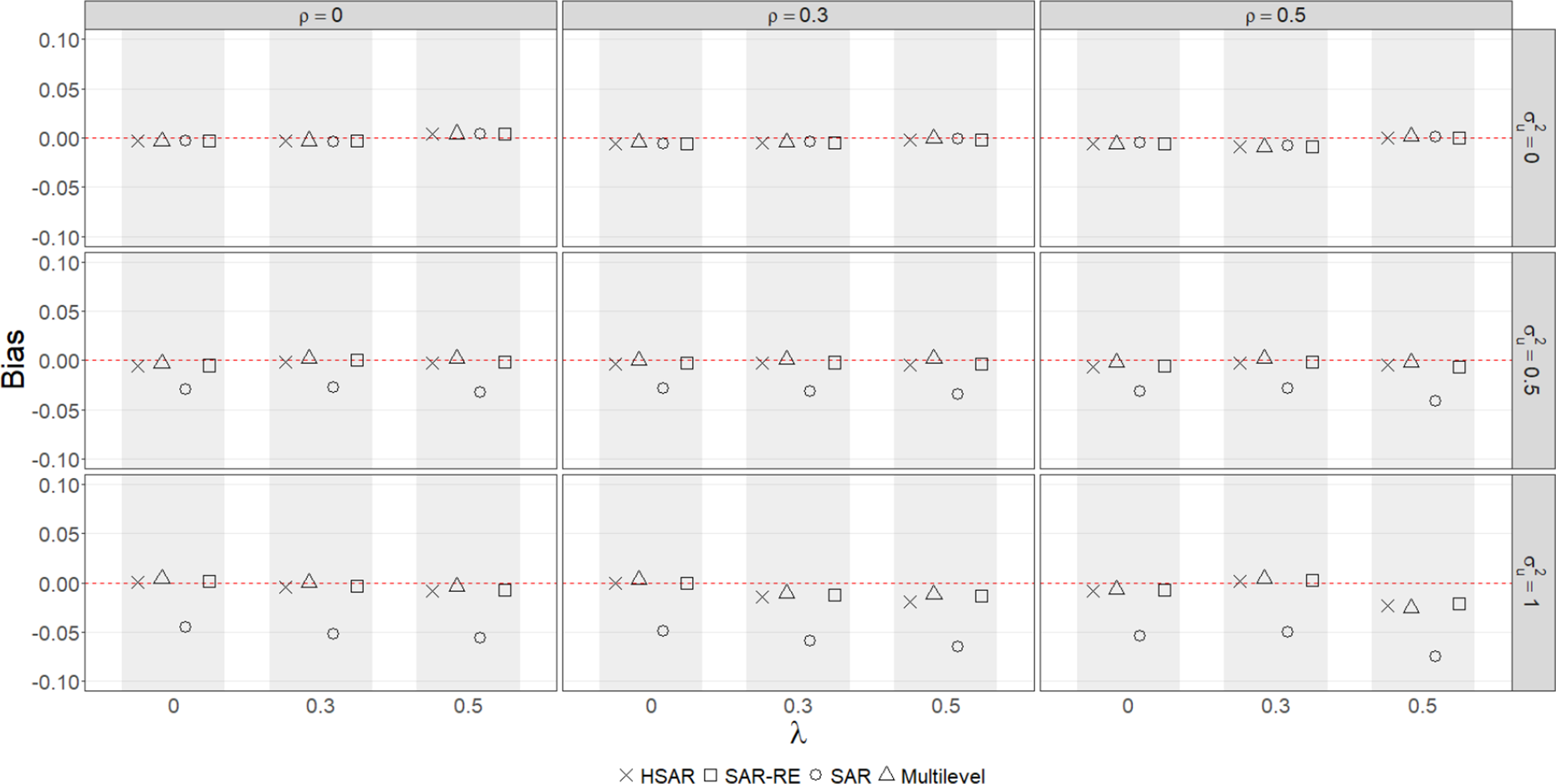
The results from our simulations are consistent with our expectations. In Figure 1, although the SAR probit model performs well when $\sigma ^2_u = 0$ , there is attenuation bias in the direct effect of the SAR probit model when $\sigma ^2_u> 0$ . The severity of this bias increases as $\sigma ^2_u$ increases and as $\lambda $ increases when $\sigma ^2_u = 1$ . The SAR probit model also underestimates the direct effect when there are independent group-level random intercepts, i.e., $\lambda = 0$ and $\sigma ^2_u> 0$ . Overall, the HSAR, the SAR-RE, and the multilevel probit models perform similarly well.²²

Figure 1 Bias in the direct effect of $X_1$ for $J = 111$ and $N = 1,117$ .

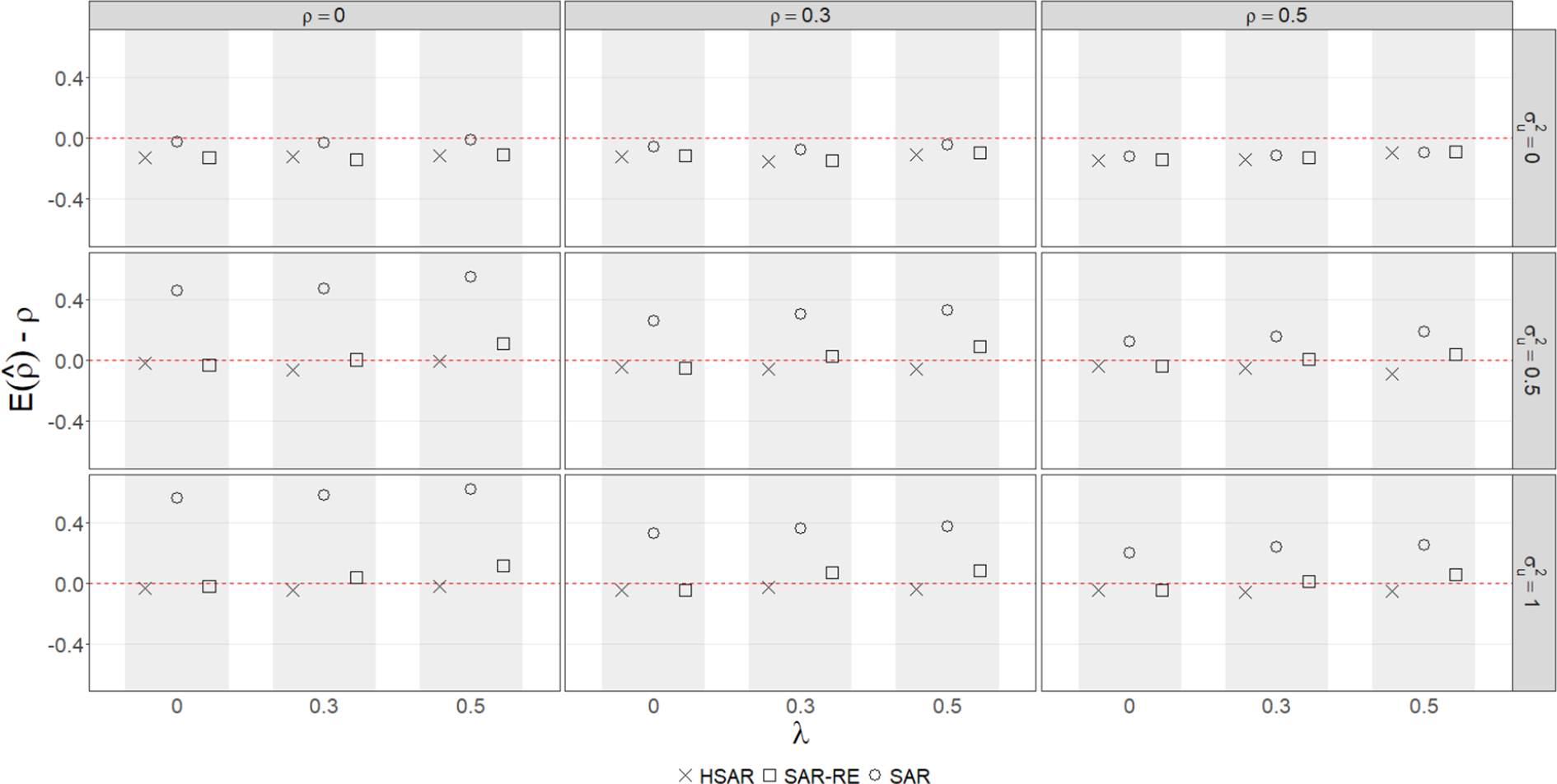
We present the results for the bias in the indirect effect in Figure 2.²³ As expected, we find that the SAR probit model performs the worst and overestimates the indirect effect when the DGP contains unobserved effects, $\sigma ^2_u> 0$ . This bias increases as $\sigma ^2_u$ increases and/or as $\lambda $ increases when $\sigma ^2_u> 0$ . We also find that the performance of the SAR random effects model’s performance worsens as $\lambda $ increases when $\sigma ^2_u> 0$ . This is consistent with our expectations as discussed in Equation (2) in Section 5.1. Our HSAR probit performs consistently well across the different combinations of $\rho $ , $\lambda $ , and $\sigma ^2_u$ .

Figure 2 Bias in the indirect effect of $X_1$ for $J = 111$ and $N = 1,117$ .

As previously mentioned, since the SAR probit and SAR random effects models do not account for diffusion among the higher-level units, they mistakenly attribute this process to the spatial process among the lower-level units. This means that the SAR probit and SAR random effects models overestimate $\rho $ , thus resulting in inflated indirect effects estimates. The results in Figure 3 corroborate these expectations. We find that the bias in $\hat {\rho }$ for the SAR probit and SAR random effects models increases as $\lambda $ increases when $\sigma ^2_u \neq 0.$ ²⁴ For the SAR probit model, it is worth noting that we observe biased estimates of $\rho $ even when $\lambda = 0$ —i.e., there is no spatial process among the higher-level units because omitting random intercepts ( $\sigma ^2_u>0$ ) is sufficient to induce bias (Cramer 2003; Neuhaus and Jewell 1993). Overall, we find that our HSAR model still performs the best in terms of $\hat {\rho }$ . These findings highlight the importance of the indirect effects in particular, when comparing the HSAR model and the SAR-RE when $\lambda , \sigma ^2_u>0$ . The HSAR model performs well because it accounts for the multilevel nature of the data and the diffusion among unobserved group effects. The SAR and SAR-RE (despite its ability to recover overall unbiased direct effects) models recover biased $\hat {\rho }$ and consequently biased indirect effects because of their inability to account for the multilevel nature of the data and level-2 diffusion by restricting $\lambda = 0$ , respectively. We also show that when $\lambda , \sigma ^2_u> 0$ , the HSAR model, on average, outperforms the SAR-RE in terms of correctly classifying events and non-events (Appendix S, Table S109 in the Supplementary Material).

Figure 3 Bias in $\hat {\rho }$ for $J = 111$ and $N = 1,117$ .

Across the different parameter combinations in the DGP and the estimates and effects calculations, we find that our proposed HSAR probit model is the best performing when $J=111$ and $N=1,117$ . In Appendices A–L of the Supplementary Material, we vary the number of higher-level units, such that $J\in \{16, 49\}$ . From the results in these appendices, when $J=49$ , $\rho = 0.5$ , and $\sigma _u^2 \neq 0$ , we notice that all models recover attenuated estimates of $\beta _1$ . Notably, the SAR probit model performs the worst and the multilevel probit, SAR random effects probit, and HSAR probit models perform similarly and recover only slightly attenuated estimates of $\beta _1$ . However, when $J=111$ , the multilevel probit, SAR random effects probit, and HSAR probit models, overall, recover unbiased estimates of $\beta _1$ .²⁵ We also note for $J\in \{16, 49\}$ , the multilevel probit and the SAR-RE overestimate the variance of the group-level intercept, $\sigma ^2_u$ , when $\lambda \neq 0$ and $\sigma ^2_u> 0$ . $\hat {\sigma }^2_u$ for the SAR-RE is biased because it omits $\boldsymbol {\lambda M \theta }$ , implying that $\hat {\sigma }^2_u$ is also heteroskedastic since $\hat {u}$ now includes the higher-level unmodeled spatial spillovers. Consequently, the standard errors will be incorrect, which will lead to incorrect inferences. Inaccurate estimates of $\sigma ^2_u$ also cause problems estimating $\beta _0$ , $\beta _1$ , and $\theta $ , which in turn affect any inference using these parameters. The HSAR probit model overall recovers unbiased or close-to-unbiased estimates of $\sigma ^2_u$ . Based on these observations, for the HSAR model, it is likely that there is small-sample bias in $\hat {\beta }_1$ when $J=49,$ which disappears when $J=111$ .

We argue that the HSAR model should be the first step when researchers believe that there are multilevel effects in the DGP. The HSAR model estimates $\lambda $ , thus allowing researchers to explicitly theorize and test for the presence of a higher-level diffusion process. When there is no higher-level diffusion ( $\lambda =0$ ), researchers can still recover accurate estimates of the parameters and the substantive effects of interest. However, this comes at a cost to efficiency. As we demonstrate in Appendices Q and R of the Supplementary Material, the SD of the HSAR model is higher than that of the SAR-RE. If the credible intervals of $\hat {\lambda }$ encompass 0, researchers may estimate the SAR-RE instead if they also find that the credible intervals of $\hat {\sigma }^2_u$ do not encompass 0.

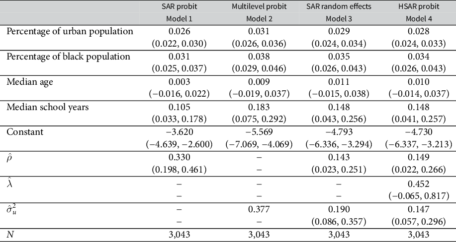
10 Application

We now demonstrate the utility of our model by analyzing the diffusion process of civil rights protests in the United States in the 1960s. There are good theoretical reasons not to overlook the diffusion process of civil rights protests. Theoretically, scholars have debated whether and to what extent protests diffuse in various contexts (e.g., Hale 2019). In the context of the U.S.’ civil rights protests in the 1960s, sociologists have pointed out various mechanisms through which protests might have spread (e.g., local newspapers, Andrews and Biggs 2006). At the same time, we argue that the potential diffusion process across states has to be taken into account for at least two reasons. First, cities and counties in different states border each other. A cursory glance of the map showing where the civil rights protests in the 1960s occurred suggests that there might have been a potential diffusion process in the baseline propensities for civil rights protests for neighboring cities and counties across North Carolina and Virginia (Mazumder 2018, Figure 1). Second, historical accounts suggest that the interstate diffusion process might be an important factor to take into account because, for example, activists traveled extensively with interstate buses as part of the civil rights movement (Andrews and Biggs 2006).

We use the dataset provided by Mazumder (2018) and investigate the potential causes of civil rights protests across the 48 contiguous U.S. states. The unit of analysis is county. The dependent variable is whether a civil rights protest took place at least once during the period, coded as 1 if any protest took place and 0 otherwise. For our covariates, we include the percentage of urban population, the percentage of black population, the median age, and the median years of school education. We estimate four models: SAR probit, multilevel probit, SAR-RE, and our proposed HSAR probit.²⁶ The multilevel probit, SAR-RE, and the HSAR probit models include state-level random intercepts. We used 50,000 iterations for the MCMC simulations and discarded the first 10,000 iterations as a burn-in.

Table 1 presents the results. The credible intervals for $\hat {\rho }$ for the SAR probit, the SAR probit with random effects, and the HSAR probit models do not encompass 0, suggesting that there is a spatial diffusion process of civil rights protests among counties. However, we notice that the estimate of $\rho $ from the SAR probit model is very large compared to the estimates from the SAR random effects and the hierarchical spatial probit models. This is consistent with our simulation results; the spatial probit model often overestimates $\rho $ .²⁷ We also notice that the SAR random effects and the HSAR models perform similarly, a result we also find in our simulations for smaller sample sizes of the higher-level units (Appendices A–L of the Supplementary Material). 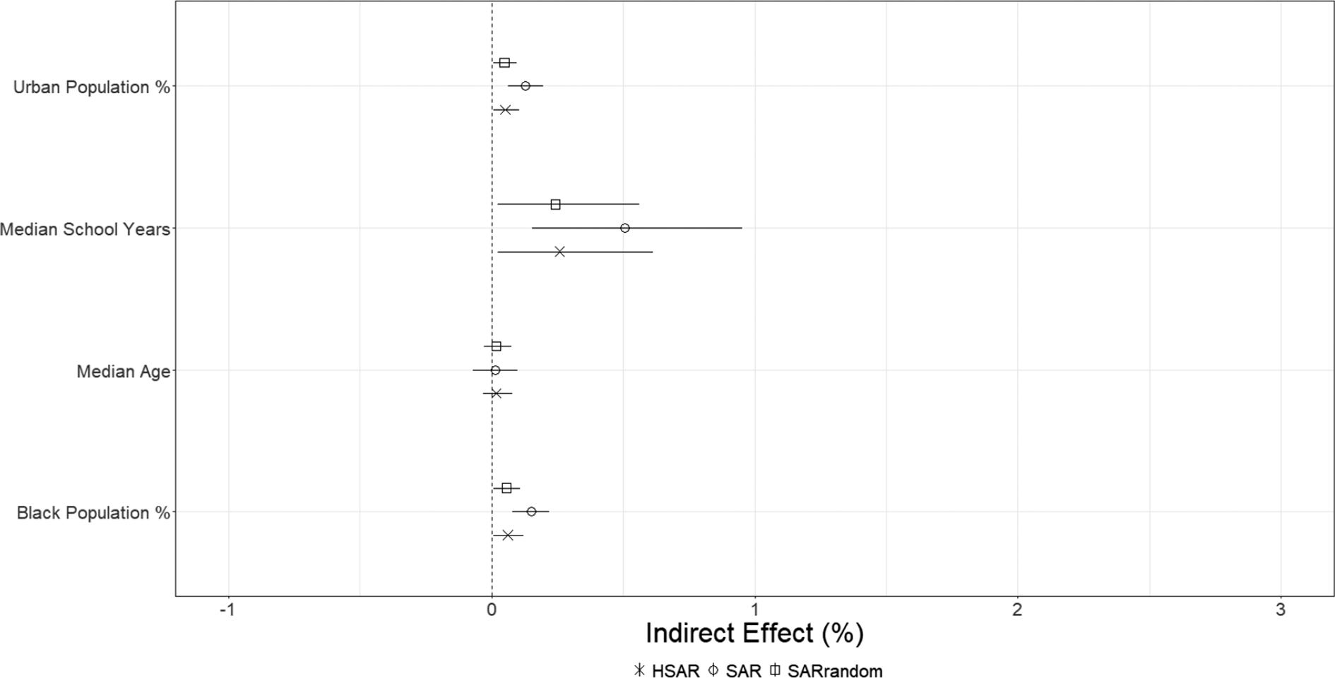The credible intervals for $\hat {\lambda }$ encompass 0 implying that we fail to find sufficient evidence in favor of the presence of diffusion in the baseline propensities for civil rights protests across states. The results from this analysis on this single sample thus suggest that only a lower-level spatial diffusion process across countries occurs. It is noteworthy that the estimates from both the SAR random effects and the HSAR probit are similar and researchers would reach similar conclusion regardless of the model estimates.²⁸ This is also evident in the direct and indirect effects shown in Figures 4 and 5. We would like to remind readers that the HSAR probit is advantageous in that it explicitly models the higher-level diffusion process, and thus allows researchers to test theoretical propositions about higher-level diffusion processes.

Table 1 Comparison of models (48 states).

Note: 95% confidence intervals for the multilevel probit model and credible intervals for the spatial models are shown in parentheses.

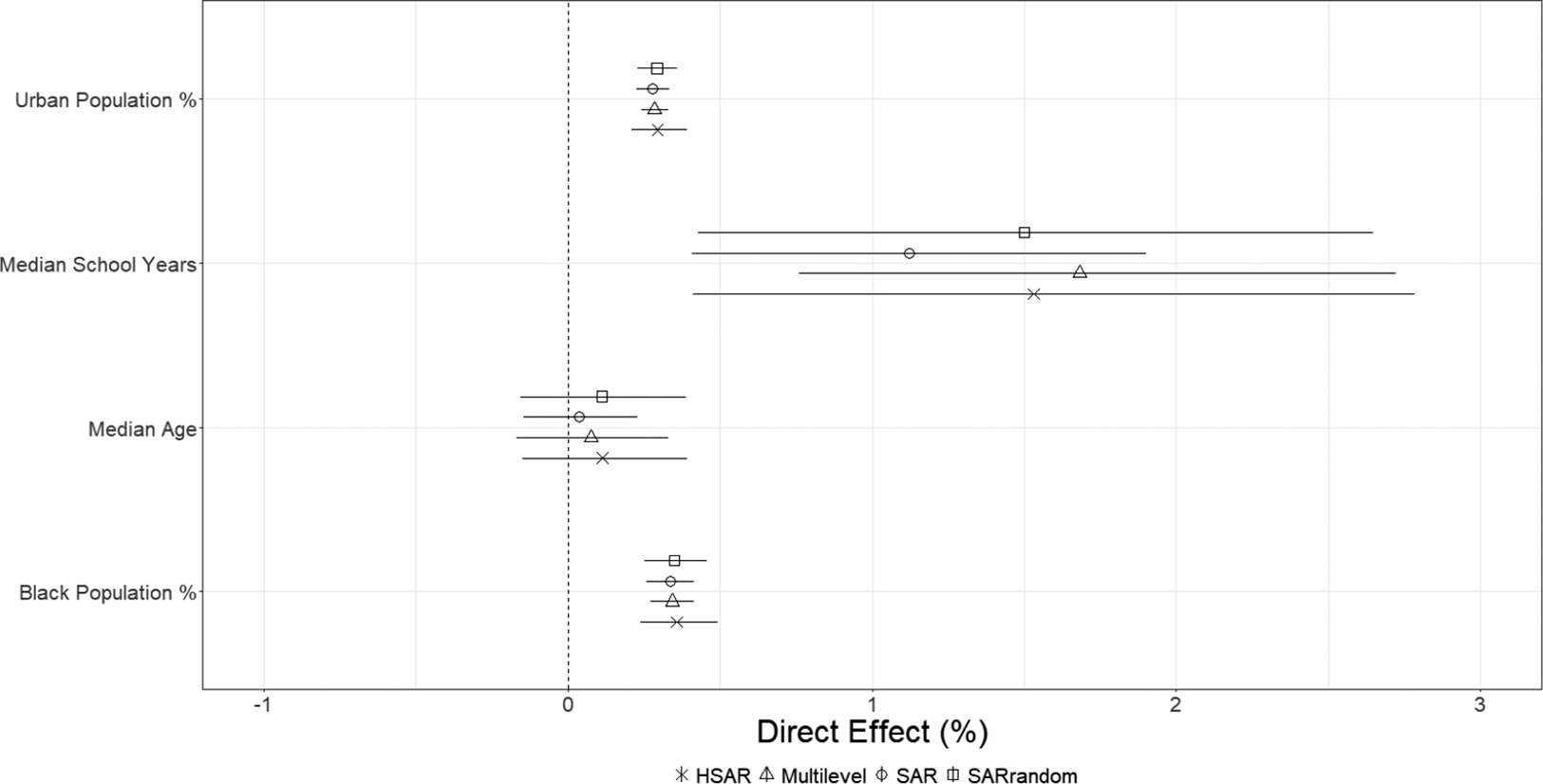
Figure 4 Average direct effects of predictors.

Figure 5 Average indirect effects of predictors.

The coefficient estimates of the predictors by themselves are not very informative about their effects because a change in a predictor in one unit affects its own outcome and also those of other units. We thus present the estimates of the direct and indirect effects in Figures 4 and 5, respectively.²⁹ For the HSAR probit, in terms of the direct effect, a 1 percentage point increase in the urban population is, on average, positively associated with a 0.3% increase in the probability of a civil rights protest occurring in the same unit. For the indirect effect, a 1 percentage point increase in the urban population is, on average, positively associated with a 0.05% increase in the probability of a civil rights protest occurring in other units. The credible intervals of the HSAR model for both these effects do not encompass 0. In general, we see that the multilevel probit, the SAR random effects probit, and the HSAR probit models provide similar estimates for the direct effect. This is consistent with what we found in our simulations. In terms of the indirect effect, we see that the SAR probit model’s estimates are in general much larger than those of the SAR random effects probit and the HSAR probit models. This is consistent with our argument around Equation (2) and the findings from our simulations.

11 Conclusion

We combine advances in spatial econometrics and multilevel modeling to introduce a class of binary outcome models, the SAR-RE and the HSAR models, that account for level-1 diffusion and spatially dependent or independent higher-level effects. We found that models, including the SAR-RE, that do not account for level-2 diffusion cannot accurately capture the spillover effects of a change in a predictor and lead to inaccurate inferences. Our proposed HSAR model, however, has widespread applicability because many datasets in political science are nested and can potentially have diffusion processes at multiple levels. Inefficiency is the only cost of estimating the HSAR model when: 1) there is no spatial diffusion, 2) there is spatial diffusion only at the lower level and there are no random intercepts, 3) there is spatial diffusion only at the lower level along with group-level random intercepts, 4) there is spatial diffusion only at the higher level, or 5) there is spatial diffusion at both levels. This is because our proposed HSAR probit model nests the aforementioned scenarios. However, when there are only spatially independent unobserved group effects, the SAR-RE outperforms the HSAR model because of gains in efficiency by estimating one less parameter.

We conclude with some practical recommendations for applied researchers. If researchers have a theory about a spatial spillover, but suspect that there is likely to be dependence in outcomes due to unobserved group effects because of the nested structure of the data, they should opt for our proposed HSAR model. Estimating this model allows researchers to additionally test for a higher-level diffusion process even if theorized to be non-existent. That is, in addition to allowing researchers to explicitly theorize and test for higher-level diffusion, it provides an additional layer of robustness even when researchers do not theorize about such diffusion. If researchers find that there is no higher-level diffusion and that the variance of the random effects is non-zero, they should consider the SAR-RE.