Classification-informed estimation: the role of water-type clustering to improve neural network generalization for salinity and temperature estimation in coastal waters

Abstract

Sea surface salinity and temperature are essential climate variables in monitoring and modeling ocean health. Multispectral ocean color satellites allow the estimation of these properties at a resolution of 10 to 300 m, which is required to correctly represent their spatial variability in coastal waters. This paper investigates the effect of pre-applying an unsupervised classification in the performance of both temperature and salinity inversion. Two methodologies were explored: clustering based solely on spectral radiances, and clustering applied directly to satellite images. The former improved model generalization by identifying similar water clusters across different locations, reducing location dependency. It also demonstrated results correlating cluster type with salinity and temperature distributions thereby enhancing regression model performance and improving a global ocean color sea surface temperature regression model RMSE error by 10%. The latter approach, applying clustering directly to satellite images, incorporated spatial information into the models and enabled the identification of front boundaries and gradient information, improving global sea surface temperature models RMSE by 20% and sea surface salinity models by 30%, compared to the initial ocean color model. Beyond improving algorithm performance, optical water classification can be used to monitor and interpret changes to water optics, including algal blooms, sediment disturbance or other climate change or antropogenic disturbances. For example, the clusters have been used to show the impact of a category 4 hurricane landfall on the Mississippi estuarine region.

Impact Statement

Understanding sea surface temperature (SST) and salinity (SSS) is critical for monitoring ocean health, particularly in coastal regions where marine heatwaves, eutrophication, and freshwater influx impact ecosystems and coastal communities. However, traditional regression models struggle to generalize across geographically diverse regions, often misinterpreting conditions in data-scarce areas like the Global South. Our study addresses this challenge by integrating a K-means clustering algorithm into ocean color models to classify water types based on spectral and spatial features, independent of location. This approach improves model accuracy by narrowing the range of SST and SSS predictions within each cluster, reducing location-specific biases. For example, the model can correctly distinguish upwelling zones or low-salinity plumes in previously unseen regions, improving global applicability. The use of K-means clustering, rather than computationally intensive convolutional neural networks (CNNs), enables large-scale, long-term ocean monitoring with lower computational demands. This democratizes access to advanced data analysis for researchers and institutions with limited resources, particularly in developing countries, while also reducing the carbon footprint of processing large Earth observation datasets.

1. Introduction

Ocean temperature and salinity are the main properties that control water density, and with it, water column stability. These properties affect biological activity directly as physiological drivers and stressors, and indirectly by controlling the spatial distribution of nutrients, dissolved oxygen and prey (Lee and Gentemann, 2017; Thakur et al., 2018). Understanding and monitoring water temperature and salinity is crucial, especially in the coastal ocean, where climate change is increasing the frequency and intensity of marine extreme events including marine heat waves (Li et al., 2022; Dai et al., 2023), leading to increased thermal and freshwater stratification (Li et al., 2020), eutrophication (Breitburg et al., 2018), and hypoxic events (Altieri and Gedan, 2015).

Multispectral ocean color models, trained using in-situ data enable monitoring of these essential climate variables (ECVs) at the required high spatial and temporal resolution (Muller-Karger et al., 2018; Medina-Lopez, 2019; Bergsma and Almar, 2020; Hadjal et al., 2022), particularly in coastal waters, where there is a mixture of complex natural and anthropogenic influences at smaller spatial scales: river plumes provide influxes of organic and inorganic material as well as pollution, upwelling over the shelf break provides cooler nutrient-rich water, and coastal habitats such as reefs and mangroves host complex and highly productive ecosystems (Dickey and Bidigare, 2005; Salisbury et al., 2011; Fournier et al., 2016).

However, ocean color models predicting sea surface properties such as sea surface salinity (SSS) and temperature (SST) from satellite images are usually trained using point-wise ground-based in-situ temperature or salinity data (O’Reilly and Werdell, 2019; Wei et al., 2023). Learning relationships between spectral signatures and water column constituent concentrations (Cael et al., 2020; Casey et al., 2020; White et al., 2024). This works at pixel level and does not include any neighborhood information which can inform on spatial distribution of features. The result is a loss of spatial information of the final product.

Applying a clustering or segmentation approach to the input image can capture this spatial information by relating pixels to each other by spectral similarity or proximity. This paper determines how using unsupervised learning to create clusters for water classification improves the performance of ocean color regression models through appropriate algorithm selection as well as retaining spatial information.

Ocean color remote sensing can be generally split into case 1 and case 2 waters. Case 1 waters are waters where the Inherent Optical Properties (IOPs) are dominated by phytoplankton, found mostly in blue open ocean waters. Case 2 waters are all others, where the IOPs are influenced by Color Dissolved Organic Matter (CDOM) and inorganic particles (Matsushita et al., 2012). Effects of the accuracy of ocean color algorithms have been shown to be reduced in highly turbid, low salinity waters (found in sediment-high rivers), as well as those in colder waters with ice mixing (Giannini et al., 2013; White et al., 2025). Classification, therefore, can be a useful tool to select the appropriate ocean color algorithms and atmospheric correction model to be applied in a certain water type (Frouin et al., 2019). Several optical water type classifications have been proposed based on surface relectance spectrum (Moore et al., 2014; Spyrakos et al., 2017, 2018). Empirical ocean color algorithms depend on inter-relationships of in-water optical constituents which change as a function of space and time in optically complex waters, therefore different spectral band algorithms are needed in different water types (e.g. highly turbid regions) to accurately estimate IOPs. Classification has been shown to improve accuracy of inversion of Chlorophyll concentration through thresholding and model selection (Sun et al., 2014; Brewin et al., 2015).

In addition to improving algorithm performance, optical water classification has also been used to monitor the size and location of water types and hazardous events, such as harmful algal blooms (Medina-López et al., 2023). To that purpose these clusters can also be used purely for ocean type monitoring, by viewing cluster size and frequency change over time. This was applied in this paper in test regions to map inter-annual changes and was able to identify changes in estuarine plume size corresponding to damming upstream.

This study aims to improve the accuracy and robustness of predictive models applied to global ocean color data, as well as case studies in the Gulf of Mexico and the UK. The datasets exhibits significant variability due to diverse environmental conditions, ranging from freshwater regions to highly saline open ocean areas. To address this challenge, we employ K-means clustering to group water samples into distinct water types. Each cluster represents a specific environmental context, such as coastal, open ocean, or transitional zones.

This paper is structured as follows: i) introduce the ground-truth datasets (buoy data) and Sentinel-2 satellite imagery; ii) select the clustering algorithm and hyperparameter, iii) apply clustering algorithm to the spectral band point data, and then regions of the image that resulted from image segmentation iv) show results for the locations of the different cluster classes, as well as the dynamics between average spectral band for each cluster and the matching sea surface temperature and salinity cluster distribution.

2. Materials and methods

2.1. In situ and satellite datasets

This section introduces the matched in-situ and satellite data for two independent datasets from the UK and the Gulf of Mexico, as well as global SST and SSS from the Copernicus in-situ monitoring system (CMEMS TAC Data Team, 2021).

The global in-situ dataset comes from the Copernicus in situ Marine Environmental Monitoring Service (CMEMS) (with datasets coming from over 100 countries (European Commission, 2023). CMEMS provides pointwise data from various observing systems, including Argo float profiles, and observations from ships, moored buoys, drifting buoys, fixed platforms, gliders, ferry-boxes, and coastal observations (SeaDataNet, 2025). The Gulf of Mexico was chosen as a study region for its varied waters, including shallow coastal bays and deeper offshore regions, which provide an excellent opportunity to study the dynamics of coastal ecosystems. These areas are characterized by their proximity to land, complex bathymetry, and diverse marine habitats. The Gulf of Mexico Coastal Observing System (GCOOS) uses NOAA cruises and stations to monitor estuaries in the Gulf of Mexico (Jochens and Watson, 2013). UK smart buoy data is obtained from the Centre for Environment, Fisheries and Aquaculture Science of the UK (Cefas; Cefas, 2024).

The satellite used in this study is the European Space Agency (ESA) Sentinel-2 multispectral satellite system. Consisting of two satellites, Sentinel-2A and Sentinel-2B, it offers a revisit time of approximately 5 days at the equator, enabling frequent monitoring of Earth’s surface in a polar orbit with a pixel spatial resolution of 10 m $ {}^2 $ . The Sentinel-2 data comprise 13 spectral bands, each represented as 16-bit unsigned integers (UINT16) and scaled by a factor of 10,000 to obtain top-of-atmosphere (TOA) reflectance values. The spectral bands include: coastal aerosol (443 nm), red edge detection (705 nm) and near infrared band (842 nm), and a full list is available here: (European Space Agency, 2023).

2.2. Ocean color model

All of the in situ datasets underwent the same matching process with the multispectral satellite images. The Sentinel-2 data was processed on the Google Earth Engine Python API platform. This allows geospatial analysis and processing of satellite images on Google Cloud computers, using scalable, high-performance computing resources. However, there is additional data transfer costs and the inherent risks from depending on a third party provider (Google Earth Engine, 2023). Latitude, longitude and time of measurement are taken for each in-situ data point. The Sentinel-2 image collection is filtered to the tiles that contain the point on the day and time when the measurement was taken, within one hour of Sentinel-2 overpass. One hour was chosen to improve accuracy, especially in the coastal zones where tidal effects and river flows can vary significantly over the course of hours.

The matched images for those points are clipped in 3x3 pixel windows about the in-situ data point, to retain the high resolution benefits from the Sentinel-2 satellite. The whole 3x3 pixel window is taken to avoid any random noise reflectance, wave effects or sun-glint errors occurring at the pixel level. The median value of the window for the spectral bands and metadata is then selected for the matched point. Time difference is also recorded between the in-situ measurement and satellite image, if there are multiple images within 1 hour of the in-situ point the smallest time difference is selected. The output is a table containing all satellite data (spectral bands and metadata properties) with the corresponding salinity and temperature data.

Various machine learning models were trained on the matched satellite and in-situ data with the inputs being the spectral bands and metadata and predicting SSS and SST independently as output. In this study, a feed-forward neural network architecture with multiple hidden layers (10) was designed, with a Tanh activation function to for propagating non-linearities, to capture the complex second order relationships between spectral signatures and the water physical properties. 18 nodes were used for the neural network initial layer to match the input data of bands and metadata. Dropout regularization helped prevent overfitting, while early stopping, based on validation set performance, further ensured that the model did not overtrain on the noise in the data. Additionally, the max-pooling layers, improved model ability to extract relevant information and improve generalization performance. Training the network with stochastic gradient descent (SGD) and optimizing with mean squared error (MSE) allowed for more efficient convergence over the course of 1000 epochs, resulting in a model that outperformed traditional methods like gradient boosting and XGBoost. The neural network’s ability to capture complex, non-linear dependencies between features made it the most effective approach for this study.

All models were trained using a 70% training and 30% testing data split. The training data was further subjected to k-fold cross-validation with k = 5, where the model was trained on 4 folds and validated on the remaining fold, rotating through all folds. Early stopping and hyperparameter tuning were conducted using the validation folds within this k-fold process.

The models were optimized using RMSE as the primary error metric and evaluated on RMSE, RME, MAE, and MPSE. To ensure a robust assessment of model generalizability, certain buoy locations were completely withheld from both training and validation datasets, serving as an independent test set. The figures and metrics in the results section are derived from this unseen test data, providing an evaluation of the model’s real-world performance.

2.3. Unsupervised machine learning (clustering)

Unsupervised learning, particularly clustering, is a crucial method in data analysis for uncovering intrinsic patterns within datasets without predefined labels (Caron et al., 2018). In clustering, the goal is to group similar data points based on certain similarity metrics, by optimizing an objective function, bringing coherence to the data and enabling exploratory analysis. In remote sensing, unsupervised clustering is particularly useful for analyzing multispectral or hyperspectral imagery. Algorithms like K-means help reveal patterns in spectral signatures without the need for labeled training data (Melgani and Pasolli, 2013; Naeini et al., 2014). The algorithm classifies pixels into “K” clusters based on spectral similarities, revealing inherent patterns in the data. Other clustering methods include hierarchical clustering, which builds a tree-like structure of nested clusters, iteratively merging or splitting clusters based on their pairwise dissimilarities; or DBSCAN, which identifies dense regions of data points separated by sparser areas. These approaches are particularly valuable in scenarios where labeled training data for supervised methods is scarce.

In this paper, we test four clustering algorithms: K-means, Fuzzy C-Means (FCM), Spectral Clustering, and Hierarchical Clustering.

2.3.1. K-means

K-means is a popular unsupervised machine learning algorithm used for clustering data into $ K $ distinct groups or clusters (Jin and Han, 2008). The algorithm aims to partition $ n $ data points into $ K $ clusters in such a way that the within-cluster variation (or inertia) is minimized. Given a set of data points $ X=\left\{{x}_1,{x}_2,\dots, {x}_n\right\} $ and $ K $ cluster centroids $ C=\left\{{c}_1,{c}_2,\dots, {c}_k\right\} $ , the objective is to assign each data point to the cluster with the nearest centroid, minimizing, for example, the objective function presented in Eq. 2.1. The process then iteratively assigns data points to the cluster with the nearest centroid and updates the centroid based on the mean of the assigned points. This process continues until convergence occurs, resulting in K clusters characterized by their centroids.

(1) $$ J=\sum \limits_{i=1}^k\sum \limits_{x\in {C}_i}\parallel x-{\mu}_i{\parallel}^2 $$

$ k $ is the number of clusters, $ {C}_i $ is the $ i $ th cluster, $ {\mu}_i $ is the centroid (mean) of cluster $ {C}_i $ .

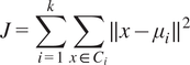
K-means is simple and easy to implement and can result in fast convergence. However, the effectiveness hinges on the appropriate choice of K, which can be determined by silhouette analysis, or the elbow method to find the optimal number of clusters (Yuan and Yang, 2019; Umargono et al., 2020). Silhouette analysis gives an idea of the separation distance between resulting clusters (Wang et al., 2017). The silhouette coefficients have a range from (SeaDataNet, 2025) with +1 indicating the sample is far from the neighboring clusters and − 1 indicating a datapoint may be assigned to the wrong cluster. It can as well be sensitive to the initial centroid locations, therefore validation methods such as K cross fold validation are useful to avoid fitting local minimums (Mayo, 2022).

2.4. Clustering for classification of water types

Two main methodologies are tested in this paper. The first approach undertakes clustering purely on spectral radiances. Although this does not contain spatial information, this helps improve the generalization of the models by learning similar clusters in unfamiliar test locations, reducing location dependencies: e.g. if the water classification in a region in Patagonia with no in-situ training data is the same as a UK region with ground-truthed data, the model will infer similar distributions of sea surface properties improving regression estimations.

The clustering of the matched satellite data was done solely using the spectral bands as inputs to the clustering algorithms. Different clustering methods were trialed, K-means, Fuzzy C-means, Spectral clustering, and hierarchical clustering. K-means was selected due to the computational speed and resistance to outliers, good scalability and only needing one hyperparameter: K, the number of clusters. Principal component analysis (PCA) was applied to the 13 spectral bands, for dimensionality reduction, improving estimations with noise and effectiveness of the K-means clustering (Ding and He, 2004), with 95% and 99% variance resulting in 1 and 4 resultant bands respectively.

The number of optimal clusters (K) was determined, using a mixture of silhouette analysis and the elbow method. The 99% variance PCA with number of cluster of 9 had the highest silhouette score with 0.99. Figure 1 shows the silhouette plot for each cluster in the 9 cluster selection, as well as the visualization of the clusters for the first two features (B1 and B2). This also corresponded with distinct corners on the Elbow method graphs for both inertia and distortion. Other studies on water type classification, set 21 clusters for water types of which 9 were selected for coastal waters so our value of 9 agrees with this decision (Spyrakos et al., 2018).

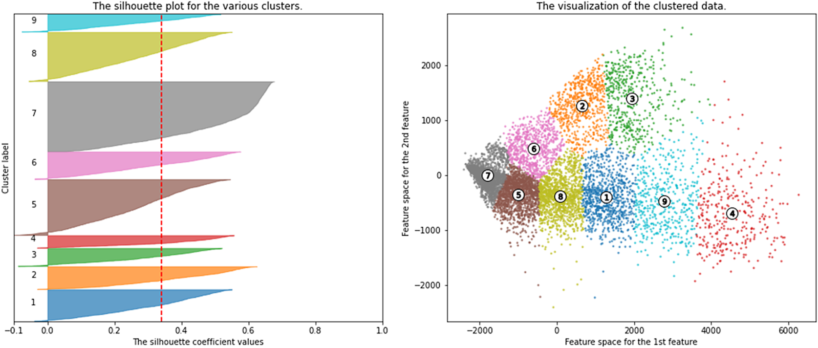
Figure 1. Silhouette score and cluster visualization for number of clusters = 9. Feature space visualization for first and second principle components with PCA variance 99% (number of components = 5).

K means clustering can be done in a number of ways—here the models are trained on pointwise matched spectral data from Sentinel-2. Latitude and longitude data were not used in the K means model to avoid overfitting problems and the model not being able to extrapolate to unseen locations. Furthermore, the link between location and SSS and SST is not often first order—e.g. a fresh water river further south maybe colder and fresher than “typical” sea water, so this location data could hinder the later model accuracy.

2.5. Image-based clustering approach

The first approach applies K-means clustering to the matched pointwise spectral data, which while separating the data into spectra based types such as seen from water color e.g. brown estuarine sediment, does not contain any spatial information from the satellite image. The second approach applies the clustering directly to the satellite image to incorporate the spatial information throughout the models. The image was segmented into distinct clusters based on proximity as well as spectral coherence. As before these clusters reduced variability of the SST and SSS distributions for each cluster, but also allowed for identification of front boundaries which can be fed into the model training alongside gradient information.

K means uses image neighborhood data based on the similarity between pixels—this means that although location data is not included—two pixels which are close together can be grouped in the same class. This is useful for the model to pick out water features such as a river plume or an upwelling—which have distinct SST and SSS properties. While we explored the Segment Anything Model (SAM) (Kirillov et al., 2023), we encountered challenges when applying it to multispectral Sentinel-2 image data. SAM, originally trained on RGB images, struggled to adapt effectively, resulting in numerous overlapping segments—particularly in ocean regions. Additionally, we experimented with convolutional neural networks (CNNs), but due to the absence of ground truth for the clusters, the computational costs outweighed the potential benefits.

First the satellite image, if coastal, used Sentinel-1 radar to mask out any land. K-means with 9 clusters were trained on $ > $ 100 satellite images, covering a full range of seasonality, coastal environments, and latitudes. The matched satellite image, with an overpass time within one hour of an in-situ ground truth measurement, was clipped to 1 km about the measurement point to ensure the capture of any submesoscale processes and the trained K-means algorithm applied to the clipped image. The original K-means algorithm was tuned to allow more homogenous clusters to be formed. Figure 2 shows an example satellite image, with the original clustering applied (2b), this shows large amounts of speckled noise with heterogeneous clustering. Merged clustering was developed, (2c) to refine the clustering, defining a minimum cluster size (25 pixels) where clusters that are smaller than the defined minimum are identified and merged into their neighboring larger clusters. This removed some smaller noisy clusters but struggled with image boundaries and linear clusters. Dilation and erosion operations are used to merge noisy clusters, acting as a smoothing post-processing step. The “focal mode” image filtering function is used with a radius of 3 and 1 iteration for smoothing. Figure 2d shows the dilation smoothed clustering with uniform clusters agreeing with both image inspection and underlying physical processes. These all are post-processing steps to the K means clustered image. We also considered the smoothing of the input satellite image, but this increases coastal errors and reduces the benefits of the initial high-resolution satellite data.

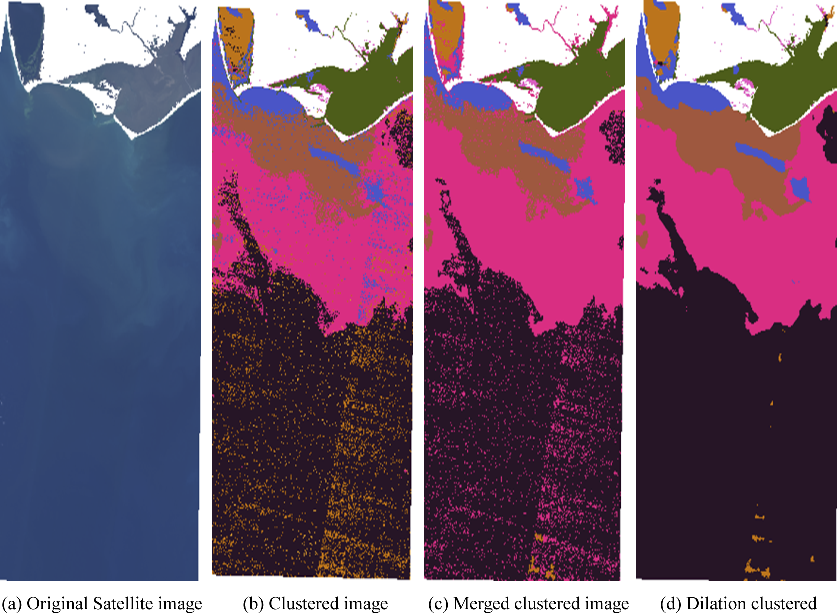
Figure 2. Clustered images, showing the coast adjacent to the Apalachicola River Wildlife and Environmental Area. With land masked in white. Clusters show agreement between different processes with less noise in the dilation clustering. a) Original Image, b) Simple clustered image, c) Merged clustered image (with minimum cluster size 25 pixels), d) Dilation smoothed clustered image.

3. Results

Figure 3 shows the locations and distributions of the image-based segmented clustering. Figure 3a shows the clustering in the Mediterranean Sea with cluster 1 as the dominant cluster. Figure 3b shows the North Atlantic coastline and the Gulf of Mexico cluster locations with a split between cluster 2 in the very coastal regions moving to cluster 1 in far shore conditions.

Figure 3. Cluster spread from the Global dataset focused on the Mediterranean (a) and the North-West Atlantic coast and Gulf of Mexico (b).

Figure 4 shows the 3D visualization for the 9 clusters against the input features, (e.g., B3, B2, B1, and other combinations). Figure 4a shows the visualization for the K-means algorithm purely done on spectral bands. There is clear cluster separation in B3 to B7, showing the link between ocean color and cluster class, compared to the noisier variables in the SWIR range. Figure 4b shows the visualization of the bands for the image-based K-means, while there is a similar separation of the features by cluster it is less defined showing the reliance of the image-based algorithm on other input features such as neighborhood information.

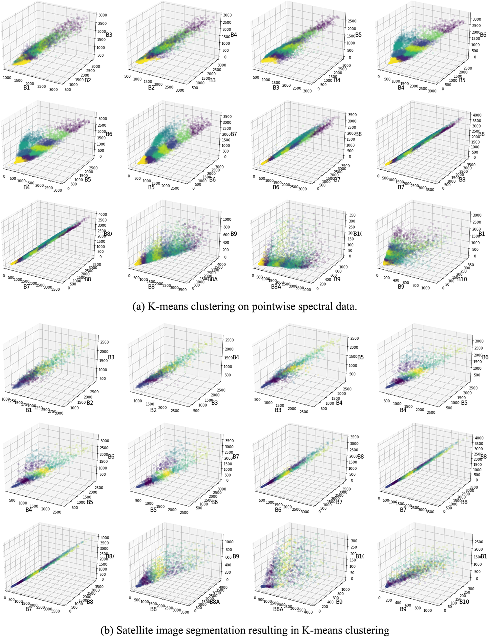
Figure 4. K-means clustering shows the different cluster classes against different input feature groups, enabling visualization of the feature weight and spectral variability to the classified cluster. a) K-means on pointwise spectral data shows separation of clusters by band b) K-means on segmented image has less clear band importance.

Figure 5 shows the mean cluster spectra and corresponding SST and SSS distributions for the global dataset and the two case studies in the Gulf of Mexico and the UK. The case studies in Mexico and the UK waters show very correlated spectra compared to the variety of spectra seen in the global dataset. This can also be seen reflected in the kernel density functions representing the distributions for temperature in each cluster. SSS distributions vary more depending on cluster reflecting the closer link between spectra and salinity variability measurements across different oceanic regions. This follows from the close relationship salinity has with ocean color from colored dissolved organic matter and chlorophyll. The SSS distributions for clusters 1 and 2 for Mexico (Figure 5f correlate well with the locations seen in Figure 3b, with the nearshore cluster 2 having a freshwater peak compared to the more saline open ocean cluster 1. The UK region stands out, it only detected 2 classes, clusters 1 and 2. It also has extremely similar SSS kernel density functions (KDFs), due to its low variability in salinity data. Testing showed good results with Pearson correlation coefficient, cosine similarity, and spectral angle mapping all showing separations of SST and SSS distributions purely based on spectral cluster type.

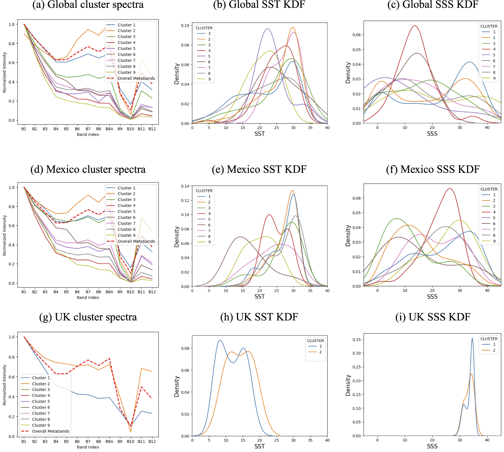
Figure 5. Spectra for the different clusters for the global dataset (a), Gulf of Mexico (d), and the UK (g), and the corresponding kernel density functions for the sea surface temperature (°C) and salinity (PSU) distributions.

3.1. Cluster impact on neural network SST and SSS prediction

The plots in Figure 6 show the spread for the neural network predicted SST against actual values for each cluster for the global dataset. Where the model is trained only on each individual cluster. By training separate models on these individual water types, we reduce the variable range within each subset. Consequently, models can achieve better performance, as they focus on more homogeneous data segments. There is an improvement overall compared to the model with no cluster data impact as seen in Table 1 which shows the model results for RMSE, R $ {}^2 $ , and the variable range for the predicted SST and SSS for original models, spectrally clustered models, and the image segmented clusters model.

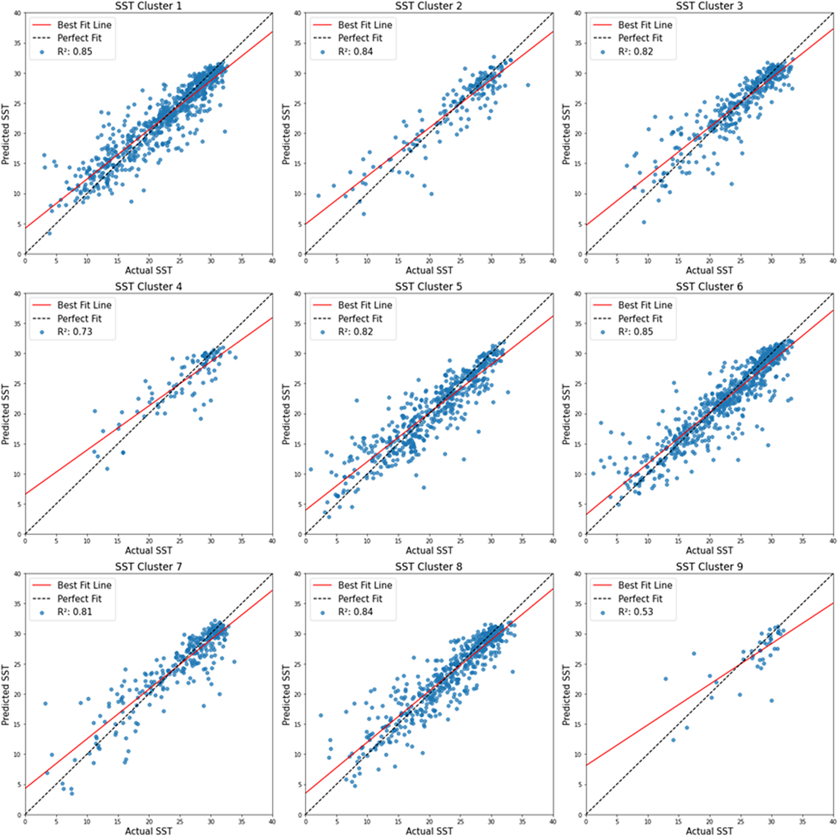
Figure 6. Global Scatter plots of predicted against actual sea surface temperature for each segmented image model trained only on the selected cluster class.

Table 1. Model performance metrics for overall sea surface temperature and salinity models, with the best-performing model per region highlighted in gray

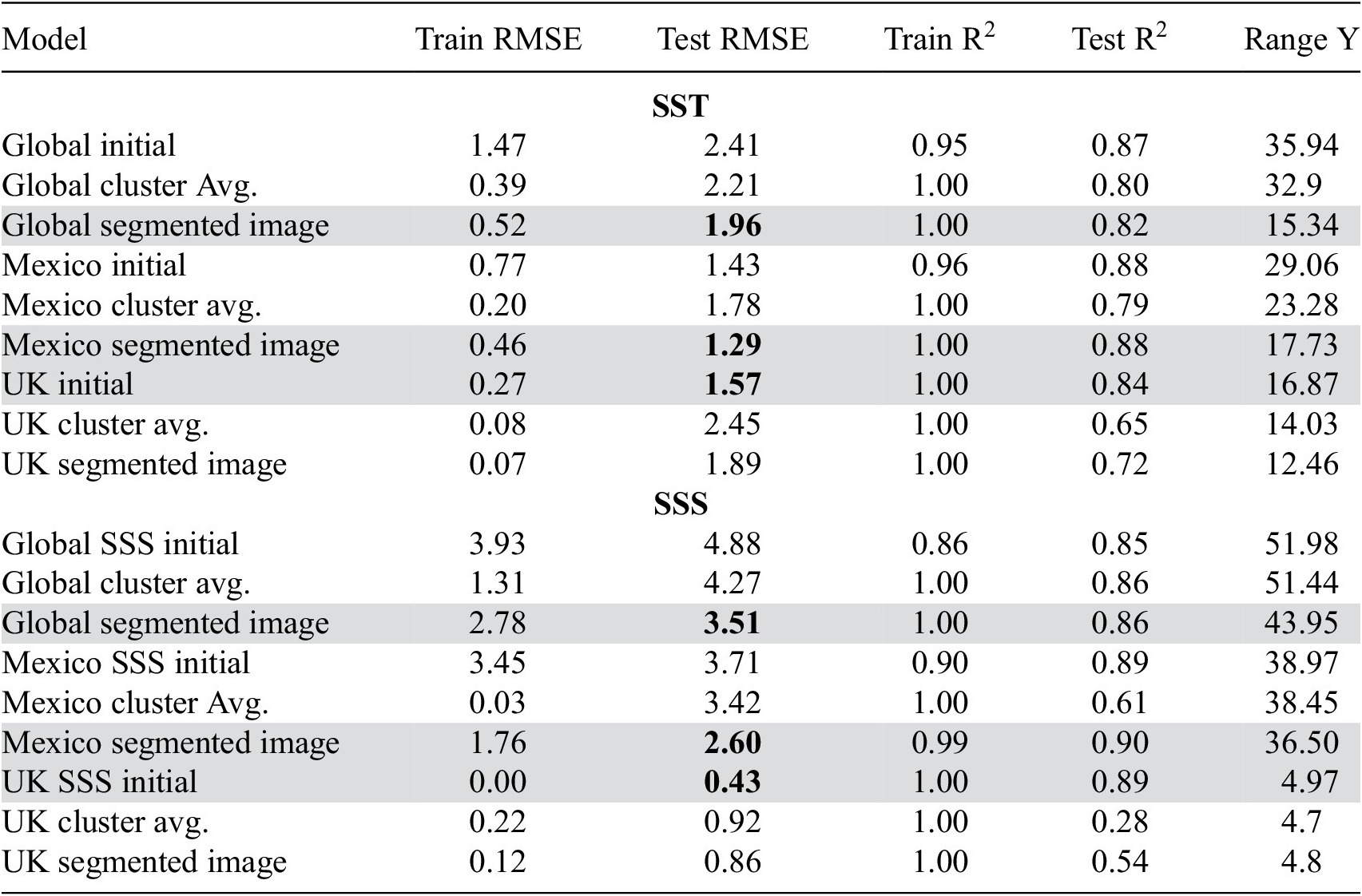
Note. Model performance metrics for overall sea surface temperature and salinity models, with the best-performing model per region highlighted in bold.

Incorporating cluster data into the training phase of regression models enhances their performance by increasing the models’ understanding of SST or SSS distributions within each cluster. As indicated in Table 1, the Root Mean Square Error (RMSE) and other accuracy metrics for the comprehensive model are presented for each location and case study, juxtaposed with the clustered data outcomes.

The spectral clustered models for SSS and SST show a reduction in Train and test RMSE for the Global and Mexico dataset. Yet the Test RMSE values are higher than the initial models for the UK locations, suggesting that while the models fit the cluster data well, they may not be capturing the variability necessary for accurate predictions on the test set. The global model benefits from a reduction in prediction set variability as does the Mexico data, but this advantage is offset by the diminished training data, which adversely affects the models for the smaller UK regions. The UK SST model shows a higher Normalized Test RMSE for the cluster average, which could imply overfitting to the cluster data or that the clustered data does not represent the broader dataset well.

The clustering based on segmentation of the satellite image, it further improves the global SST and SSS RMSE as well as aiding the Mexico result. Improving global sea surface temperature models RMSE by 20% and sea surface salinity models by 30%, compared to initial ocean color model.

3.2. Image application and visualization

Figure 7 shows a true color Sentinel 2 image compared to the clustered image. The clustering was applied to the Mississippi River outflow in the Gulf of Mexico, with the black outline showing the land and cloud masking applied to the pre-classified satellite image. The images were both taken in September, the first in 2022 (for reference of unaffected conditions) and the second in 2021, when there was significant flooding both upstream in the Mississippi delta and increased mixing due to storm winds from Hurricane Ida. As can be seen from the RGB images this flooding and storm activity has increased the size and distribution of the sediment plume. This is captured in the clustered images with the pink cluster (cluster 5) capturing the full extent of the sediment (and even some which are not visible in the true color image).

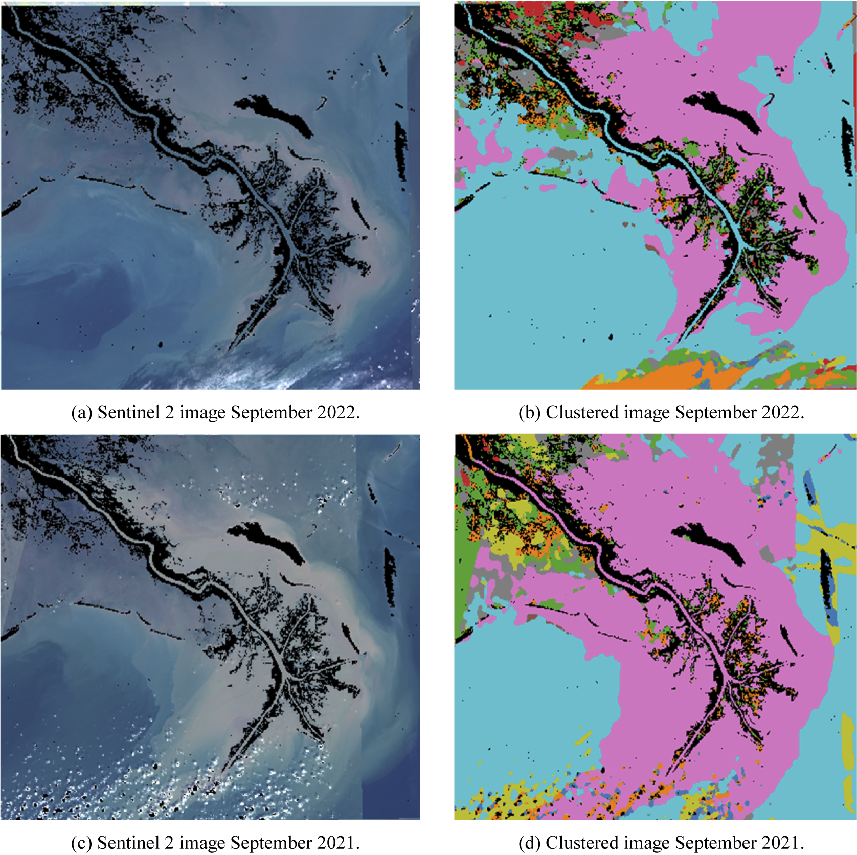
Figure 7. Cluster visualization for Mississippi outflow in the Gulf of Mexico against a true color Sentinel 2 image. The images are from September 2022 and September 2021, when there was significant flooding due to the landfall of Hurricane Ida, a Category 4 storm.

Figure 8 shows the average cluster area (in thousands of km $ {}^2 $ ) for the seasons in the years 2018–2023, in the region shown above in Figure 7. Cluster 5, as seen as the outflow class, is the most dominant in spring, but in summer, it is the 5th biggest cluster (showing the extremity of the flooding in Summer 2021 7d). In winter, with less outflow, cluster 8 (corresponding more to Case 1 open ocean waters) is the biggest class. Interestingly class 1 and class 2, appear the most in summer. These seem to be correlated with warmer, highly productive waters appearing around the delta region of the Mississippi.

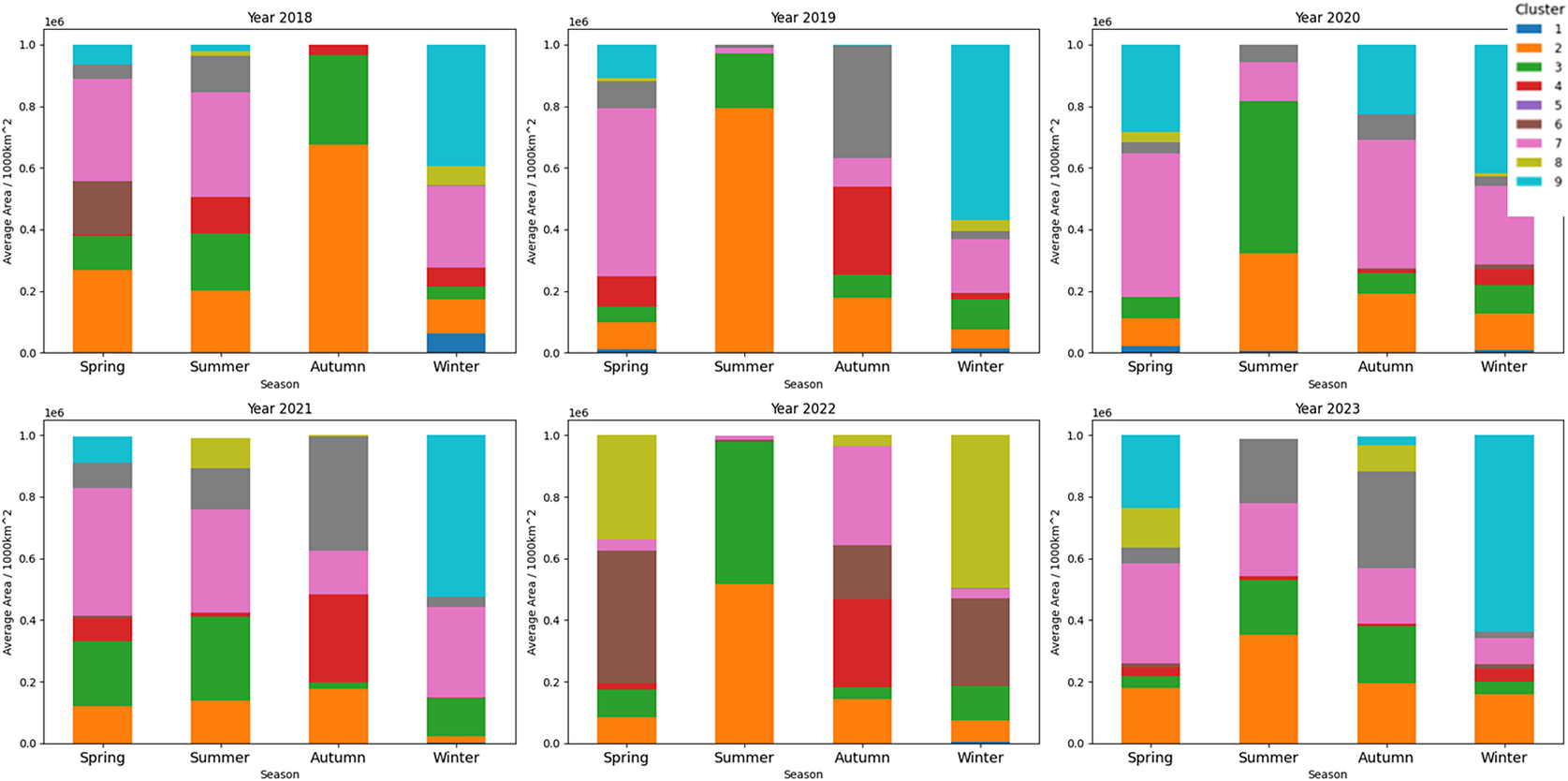
Figure 8. Cluster size for each season in the years 2018–2023, for the Mississippi outflow region is shown in Figure 7.

Figure 9 shows the correlation between the cluster classes and the SST distribution for a region in the Gulf of Mexico, there is a clear overlap between the warm cold front seen in the temperature plot compared to the plot of the cluster, which shows why there is such an improvement in the RMSE errors of the regression prediction model when the cluster spatial information is included.

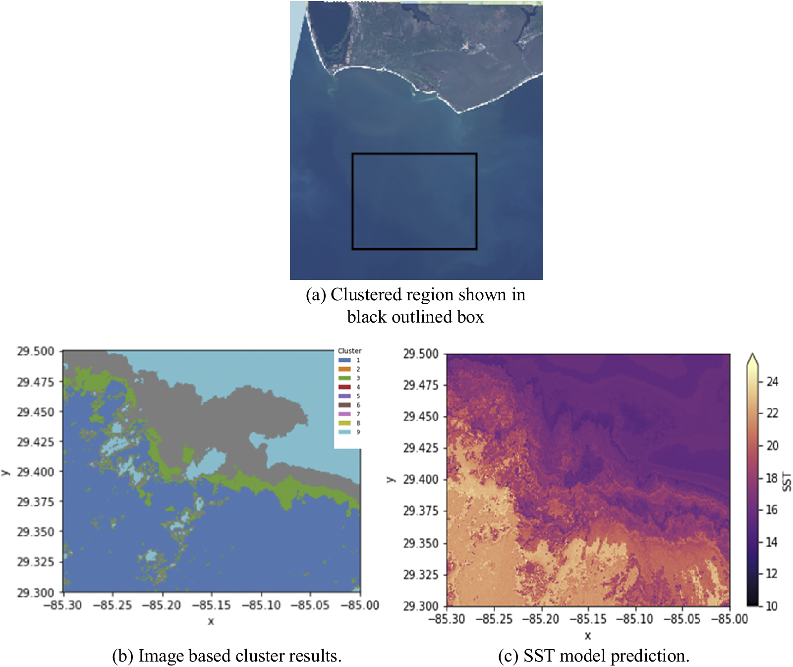
Figure 9. Cluster class vs sea surface temperature in the Gulf of Mexico test region, adjacent to the Apalachicola River Wildlife and Environmental Area.

4. Conclusion

Implementing these classification algorithms has demonstrated an improvement in the regression model’s Root Mean Square Error (RMSE), indicating enhanced predictive accuracy. Nonetheless, it is important to ensure that the training data encompasses a full distribution of all sea surface types. This comprehensive coverage is crucial for the accurate classification of specific water types. With purely spectral-based clustering, no additional information is added to the model, which is still trained on pointwise data, however, the multi-model approach can reduce the variance of each predicted variable. Applying the clustering directly to the satellite image in the segmentation approach, allows spatial information to be included in the model capturing physical processes.

The image-segmented clusters can also be used to track the impact of changes by anthropogenic or climate changes, both seasonally and interannually, to help guide policy and understand the challenges faced by ecosystems, and calculate the probability and extent of changes due to predicted climate warming.

A recurring issue with traditional ocean color temperature and salinity regression models is their inability to accurately handle regions that differ from the ones they are trained on. Specifically, when the model is used on data from a new location, it tends to incorrectly assume that the data distribution is the same as that of the training data. For instance, if the model was trained on data from the UK, it might predict an average temperature of $ 14{}^{\circ} $ C, which is typical for the UK. However, when applied to data from Mexico, where the actual average temperature is $ 25{}^{\circ} $ C, the model’s prediction could be significantly off. This can lead to skewed results due to the uneven availability of training data, particularly from regions like the Global South. Classification can help to overcome these challenges, as the clustering was not based on location, it can pick out processes such as upwelling, and identify regions such as low saline or warmer water. The overarching goal was to achieve similar types of classification regardless of geographical location. However, the pre-classification of ocean color data can introduce a significant limitation on later regression models by constraining the model’s output range. This could result in an over-reliance on simpler algorithms, such as K-means, to perform the heavy lifting of defining these constraints. Care must be taken to monitor the importance that deep learning models place on the clustering inputs (e.g., by weight tracking).

Using a straightforward K-means algorithm and feeding its results into a deep neural network model enables complex spatial and image analysis without the computational cost and processing time associated with more sophisticated algorithms, such as convolutional neural networks. It is important to note that our segmentation method, which is based on clustering, only provides an approximation of water types such as ‘river plume’, ‘turbid delta’, ‘open ocean’, and so forth Therefore, employing a complex CNN for clustering would not necessarily yield a significant improvement in accuracy. Using this K-means algorithm means that the final model can be feasibly applied to large-scale datasets as seen in earth observation problems, for long-time series mapping and then applying the vectorized results for fast processing by the deep neural network model.

By reducing the computational resources required, the model becomes more accessible to countries that traditionally have limited access to supercomputers. This democratization of data analysis can lead to more globally inclusive research and findings. Furthermore, by requiring less computational power than climate models or other deep learning structures, the model helps reduce the energy consumption associated with data processing, thereby contributing to a lower carbon footprint.

However, while this simplicity enhances accessibility, it is important to acknowledge the tension between the algorithm’s broad applicability and the constraints imposed by uneven data availability. Without sufficient regional data, especially from underrepresented regions (e.g. the global south), the model’s accuracy and effectiveness may be compromised in these regions.