When do voters reveal candidate gender preferences? Evidence from individual‐level ballot data

Abstract

Does candidate gender matter for vote choice? Whereas experimental research suggests an average preference for female candidates, observational studies tend to find null effects. In this note, we address the recent debate on how to measure voter preferences on the aggregate and the individual level. We argue that candidate gender preferences exist, but that whether and when they are revealed varies between and within voters. Drawing on an observational design and using data from over 500,000 individual ballots in Lithuanian elections, we employ multilevel regression and exponential random graph models to show how voters' candidate gender preferences are distributed across the electorate and how they vary in size and direction. We find that about half of all voters prefer either male or female candidates. Whereas preference for male candidates tends to be revealed in the first and second preference votes, preference for female candidates is first revealed in lower preference votes. Our results help explain contradictory findings in the literature and illustrate how observational data and methods can be used to assess voter preferences within electorates.

Introduction

Do voters have an intrinsic preference for male or female electoral candidates? And, if yes, under what conditions is this preference revealed? Considering the persistent under‐representation of women in political offices worldwide, these questions have motivated a highly active research agenda in political science.

Previous research results are inconclusive and to some extent contradictory. A number of studies suggest that candidate gender does not matter for voters' candidate choices in actual elections as soon as controlling for other candidate characteristics such as party affiliation and incumbency (Dolan & Lynch, 2014; McElroy & Marsh, 2010; Sevi et al., 2019). In contrast, a recent meta‐study of candidate choice experiments finds that voters, on average and across a variety of contexts, prefer women candidates (Schwarz & Coppock, 2022).

In this research note, we argue that these contradictory findings can emerge because observational studies typically only evaluate one vote choice per voter and then aggregate over the electorate, whereas experimental studies average over many choices per individual. First, observational studies may miss (latent) candidate gender preferences, especially when they are unequally distributed across electorates. Consider a hypothetical case where all voters are heavily biased towards candidates of their own gender – all women voters vote for women candidates, and all men voters for male candidates. In the aggregate results, candidate gender would not, however, appear as an important predictor for voter choice, because – assuming that women and men form a relatively stable 50 per cent of electorates – the preferences would cancel each other out.¹

Some recent studies attempt to remedy this shortcoming by exploiting the spatial segregation of electorates. They all focus on voting for ethnic minority candidates and rely on the fact that the shares of voters belonging to the respective ethnic groups vary geographically (Atsusaka, 2021; Ben‐Bassat & Dahan, 2012; van der Zwan et al., 2020). However, as electorates do not tend to be spatially segregated based on gender, such an approach is less useful for studying candidate gender preferences.

Therefore, a considerable body of research has employed candidate choice experiments to reveal voter preferences for men or women candidates. Here, respondents are presented with repeated choices between two candidates, where candidate gender – together with a range of other candidate characteristics – is randomly varied. The change in voter support when a candidate ‘switches’ genders is then assessed (see Schwarz & Coppock, 2022, for an overview). However, as Abramson et al. (2022) demonstrate, experimental effects should not be interpreted as reflecting aggregate preferences of the electorate as a whole. Since the average marginal component effect assessed in experiments averages over both the direction and the intensity of preferences, it might well be the case that only a minority of voters has preferences for, say, female candidates, but that these preferences are more intense than those of the larger share of voters that slightly prefer male candidates (Abramson et al., 2022). This can lead to incorrect interpretations of experimental effects when aiming to infer majority preferences.

Furthermore, studies focusing on individual voter preferences tend to miss variation within voters, for example, across elections or preference votes. It is plausible to assume that, for the same voter, candidate gender is more salient in one than in another election, for example, in non‐partisan contexts (Anzia & Bernhard, 2022), when voting is cognitively demanding (Crowder‐Meyer et al., 2020), or when casting lower versus higher preference votes (Mustillo & Polga‐Hecimovich, 2020; Quinlan & Schwarz, 2022).

In this note, we reconcile seemingly contradictory findings by jointly studying the distribution of candidate gender preferences on the aggregate level (variation between voters) as well as their revelation contingent on the position of the preference vote (variation within voters). To do so, we exploit individual‐level ballot data from the 2016 Lithuanian election. Lithuania employs a mixed electoral system in which the proportional representation (PR) tier is an open‐list system that allows voters to first select a party or list they vote for, and then select up to five individual candidates they support – voters can thus make five choices, which allows us to test candidate gender preferences more precisely than if only one vote choice is made.

Anonymous individual‐level ballots are a novel type of data that have, so far, mainly been utilized to understand voter preferences in referendums (Casas et al., 2023). In this note, we demonstrate how they can be used to understand the distribution of preferences regarding candidate characteristics across electorates. These data, we argue, are a suitable alternative to post‐election surveys that can potentially suffer from self‐selection, social desirability bias and misreporting, especially in complex voting decisions (Bishop & Fisher, 1995; McDonald & Thornburg, 2012). On the other hand, the data can complement one main shortcoming of experiments, as they provide an observational measure of voter behaviour in ‘real’ elections where voters have to deal with imperfect information.

We present two novel approaches to estimating the effect of candidate gender on vote choice in an observational design, employing multilevel regression models and social network analysis (exponential random graph models). First, we use the multilevel models to understand the direction and distribution of gender bias throughout the electorate. The results suggest that, while about 55 per cent of voters do not have significant preferences for either men or women candidates, almost half of the electorate do have candidate gender preferences. On average, about 29 per cent of voters prefer male candidates, whereas about 16 per cent prefer female candidates. Importantly, these shares vary across supporters of different political parties.

We then proceed to assess when these preferences are revealed, that is, the variation of gender preferences within individual voters' five preference votes. As we cannot assume independence between a voter's sequential choices – if a voter chooses a woman as a first candidate, this may well impact their likelihood to choose a man or woman candidate on the following position – we rely on exponential random graph models (ERGMs) for valued networks (Krivitsky, 2012). These networks explicitly model interdependence between observations (Block et al., 2019; Robins et al., 2007). We then estimate the incidence of male–male and female–female candidate dyads compared to mixed‐gender dyads throughout individual voters' preference votes. The findings suggest that preference for male candidates tends to be revealed within the first two preference votes, whereas a preference for female candidates is more likely to be revealed within the last three preference votes.

Our contribution is threefold: First, we explain seemingly contradictory results in empirical research on candidate gender preferences by jointly analysing voter preferences on the aggregate and the individual levels. Our findings validate experimental results in an observational design and provide an explanation for why candidate gender preferences and specifically a preference for female candidates are not always revealed in real elections. Second, we do this by drawing on evidence from Lithuania, adding empirical evidence on voter preferences in Eastern Europe to a literature that quite heavily relies on studies from the United States and Western Europe. Third, we demonstrate the use of two complementary observational methods to study voter preferences. Both approaches are – in contrast to designing experiments and/or conducting post‐election surveys – cheap and scalable and will allow future studies to exploit the fact that individual (anonymous) ballot data are increasingly available from a variety of contexts and electoral systems.

Data and methods

Our empirical analysis is based on voting data from the 2016 Lithuanian elections (see online Appendix B for more information). In the parallel mixed electoral system, 70 MPs are elected in a single PR district covering the whole country and 71 MPs are elected in single‐member districts. The PR component of the electoral system is based on the open‐list system in which voters have to select a party or electoral alliance they vote for and have an option to select up to five candidates they support (Figure B.1 shows a sample ballot).

In the analyses below, we use the ballot‐level data provided by the electoral commission indicating all candidates selected by individual voters.² Our information about the voters is limited to their respective polling stations and the party they selected. We combine this information with a candidate dataset containing candidates' gender and their party affiliation. We exclude four parties or electoral alliances with fewer than 2 per cent of the national vote due to the lack of information on the candidates of these formations. In all models, we include candidate age, logged list position, the number of parliamentary tenures that the candidate has previously served as well as two dichotomous variables indicating that (1) the candidate runs in the same single‐member constituency in which the voter is based and (2) the candidate was born in the same municipality as the one in which the voter is located as control variables. The final control variable, also dichotomous, indicates whether both the candidate and voter are on the same side of the urban–rural divide. Specifically, the variable takes a value of 1 if the candidate's place of residence and the polling precinct in which the voter cast their vote are both either in a larger urban area or in a smaller town or countryside. The variable takes value 0 if the candidate comes from a larger urban area and the voter is from a smaller town or village or vice versa.³ We define larger urban areas as the five largest cities in Lithuania with (nearly) 100,000 inhabitants. The data on the incumbency variable come from Ragauskas (2021); all other variables were coded based on the official information provided by the electoral commission.

While parties are free to select the candidate rank on the party list, candidates are elected based on the number of preference votes they receive. This leads to a significant share of candidates – 16 out of 70 in the 2016 election – to be elected by climbing up on the list from unelectable list positions on the basis of preference votes. Preference voting is quite widely used by the electorate: in our dataset, 716,397 or 61 per cent of the voters who cast valid votes in 2016 indicated preference for at least one candidate. 83 per cent of these ballots (592,209) indicated the maximum of five candidates. Online Appendix C shows the shares of female candidates selected across all 716,397 ballots.

Our sample is thus restricted to voters who select to use their preference votes, which limits the generalizability of our findings to the entire electorate. However, it is an advantage when inferring how voter preferences for individual candidates are generally shaped. Voters who decide using their optional preference votes are arguably also the group who most likely cares about candidate characteristics beyond party affiliation at all. We can, therefore, be confident that we observe actual preferences rather than random artefacts created by electoral systems where voters must support individual candidates.

Results

The distribution of gender preferences between voters

We start our analysis by fitting logit models with random effects to estimate how voter preferences for female or male candidates vary across the electorate, that is, between individual voters. The large size of our dataset means that estimating models for all voters is computationally very intense. We, therefore, present here the results for a random sample of 5000 voters.⁴

Our unit of analysis is a dyad consisting of a voter and the candidates of the party that the voter cast their vote for. Since the list of candidates by all major parties was close in size to the number of MPs (141), typically for a single voter we have approximately 140 observations. The dependent variable takes the value 1 if the voter casts a preference vote for the candidate in the given dyad. Since a large majority of voters who cast preference votes used all five preference votes, typically for a single voter there are five dyads with the value of 1 and approximately 135 dyads with the value of 0. The number of observations in this dataset used for analysis is 659,380; 3.4 per cent of these observations take the value of 1 on the dependent variable (online Appendix D provides descriptive statistics).

To infer voter preferences for female or male candidates at the voter level, we include random intercepts for voter IDs and random slopes for the gender variable. The inclusion of random slopes in the model allows for the possibility that the effect of candidate gender on candidate choice varies at the individual voter level. We argue that the direction and magnitude of this effect indicate voter bias for female or male candidates. Since our gender variable takes value 1 for female candidates, positive random slopes indicate voters' bias for the female candidates, and negative slope values indicate a bias towards the male candidates. As with the coefficients of logistic regression, exponentiating random slope values gives the odds of voting for female candidates over the odds of voting for male candidates. For example, the value of an exponentiated random slope of 1.2 means that a voter is 20 per cent more likely to vote for the female candidate than for the male candidate. Our main interest is in the distribution of random slopes across voters: they show how frequent different voter biases are in the electorate.

The regression estimates suggest that the average effect of gender on candidate choice is not statistically significant from zero (see regression estimates in online Table D.2). Apart from candidate age, which is also not statistically significant, other variables have expected effects: candidates in higher list positions and with greater incumbency experience as well as candidates who share single‐member districts or place of birth with the voter, are more likely to win preference votes.

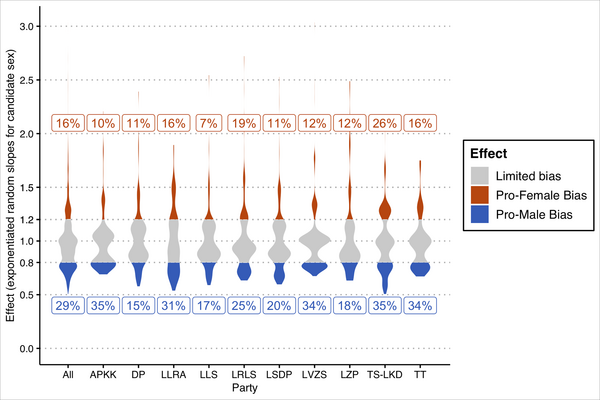
However, once we focus on the individual voter level, we observe fairly significant variation in voter biases for female or male candidates. Figure 1 reports exponentiated random slopes (thus showing the change in probability). As mentioned above, scores below 1 represent voters who prefer male candidates and those above 1 show voters who prefer female candidates. We can thus assess not only the direction of preferences but also their intensity. While both preferences for female and male candidates are present, the former exhibits greater variation than the latter. This is not surprising given that, on average, 72 per cent of candidates are male and each voter typically casts only five preference votes. To estimate pro‐male preference more precisely, one would need data where each voter selects more than five candidates.

Figure 1. Distribution of exponentiated random slopes.

Note: Estimates based on Model 1 in Table D.2. Percentages indicate the share of voters exhibiting pro‐female or pro‐male bias.

To increase the interpretability of our results, we set the threshold of the change in predicted probability of 20 per cent as indicating a significant gender bias. In setting this threshold, we follow King and Zeng (2001, 152), who consider 10–20 per cent changes in probability as important. Based on this threshold, almost one‐half of the electorate exhibits significant gender biases: 29 per cent for male candidates and 16 per cent for female candidates (see the first violin plot in Figure 1). In the models based on additional random samples (online Appendix D), these shares vary from 29 per cent to 30 per cent for male candidates and 14 per cent to 19 per cent for female candidates.

The remaining violin plots in Figure 1 show how the estimated slopes vary by party. Of most interest is the variation across the three largest parties in the 2016 parliamentary election with a combined vote share of 60 per cent. Homeland Union ‐ Lithuanian Christian Democrats (TS‐LKD; 23 per cent of the PR vote) and the Lithuanian Social Democratic Party (LSDP; 15 per cent), the two most established parties in Lithuania with the experience of leading governments, are ideologically similar to their Western European conservative and social democratic counterparts. The Lithuanian Peasant and Green Union (LVZS; 22 per cent of the vote) received the most seats in the election with an eclectic set of economically leftist, socially conservative and anti‐establishment appeals. We note that pro‐male and pro‐female biases are present among the supporters of all three parties. However, the distribution of bias is more balanced in the case of TS‐LKD: 35 per cent of its supporters had pro‐male and 26 per cent had a pro‐female bias. In the case of the other two parties, the proportion of supporters with pro‐male bias is almost twice (LSDP) or thrice (LVZS) as higher than the share of supporters with seemingly pro‐female preferences. This resonates with the findings by Ragauskas (2021), who argues that social democratic voters aimed to correct the candidate‐viability‐bias introduced by a recent gender quota.

When are gender preferences revealed?

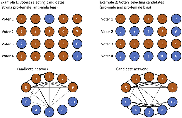
We build on these results to further analyse how voter preferences for candidate gender vary within voters, that is, across preference votes. Importantly, we cannot assume that a voter's five candidate choices are independent from each other. The sequential nature of preference voting suggests that early candidate choices might directly influence later ones. For instance, as shown in online Appendix B, few voters compose all‐male or all‐female ballots. Therefore, we apply ERGMs for valued networks, which are particularly suited for networks with count data (Krivitsky, 2012). Our dependent variable is the networks between the candidates of a party, in which every shared vote (i.e., coming from a single voter) for a pair of candidates increases the tie count by one. Thus, candidates who share strong ties have been jointly selected by a high number of voters. To further illustrate this, Figure 2 shows two examples with only four theoretical voters, and each voter indicates five preferences for candidates from a list of 10. The first example (left‐hand side of the figure) represents a case where a majority of voters have a strong preference for female candidates. The first voter selects candidates 1, 3, 2, 7 and 9 (in that order), and for each of these candidate pairs in the network the tie count increases by one. This is done over all voters to construct the candidate networks. The resulting network shows that there are many (strong) ties among female dyads (in this example, the combined tie count is 25), while male dyads are only very loosely connected (tie count 1). Mixed dyads have a joined tie count of 15. In such an example, the ERGM – using the mixed dyads as the baseline – is expected to exhibit a strong positive coefficient for female dyads, and a strong negative coefficient for male dyads. The second example shows a situation where some voters have preferences for women, while others prefer men. In the resulting network, we see two clusters emerging, with a high combined tie count for both female and male dyads (16 each), and the two clusters only loosely connected to each other (the tie count of mixed dyads is 8). Again setting mixed dyads as the baseline, an ERGM model in such a case is expected to exhibit two positive coefficients for female and male dyads.

Figure 2. Graphical representation of tie formation based on voter choices.

Note: In the two examples, four voters elect five candidates each. The candidates are shown as circles, with red circles representing female candidates, and blue circles male ones. The numbers in the circles denote list positions. When one voter selects two candidates, their tie count increases by one. Below the voters' choices, the resulting networks are shown. Line thickness indicates higher tie counts. The first example shows a preference for female candidates across voters; the second example shows half the voters preferring women and the other half preferring men. A higher number of voters would increase all tie counts, but if preferences are stable across voters, the general patterns remain the same.

To model our networks, we rely on the ergm package developed in R and on a maximizer to the pseudolikelihood function to estimate the models (Hunter et al., 2008). We construct networks in the above‐described way over all voters of the largest three parties in the 2016 parliamentary election with a combined vote share of 60 per cent: the LVZS, TS‐LKD and the LSDP. We model these three networks independently of each other since there are by construction no ties between candidates of different parties (candidate selection is strictly limited to within parties). These networks then serve as the dependent variables in our ERGM models (Cranmer et al., 2017).

The models aim to explain the number of ties in the network based on a set of specified exogenous and endogenous variables. Our main independent variable is again gender, which we model using the ‘differential homophily’ approach (Morris et al., 2008). This allows us to estimate the unique propensity of both genders to form ties, compared to the mixed gender dyads. Positive coefficients indicate a higher propensity of voters to jointly choose male/female candidates, compared to mixed dyads, while negative coefficients indicate that sharing the same gender has a negative impact on joint candidate selection by voters. As control variables, we include the same set of covariates as in our first approach.⁵

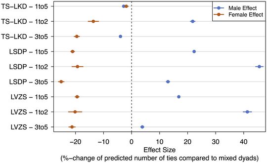
In addition, we include two endogenous terms to the models, that is, characteristics that are specific to the structure of the networks. First, we include the sum argument, which estimates the general likelihood of tie formation in the network and is equal to including an intercept in conventional regression models. Second, the nonzero argument estimates the likelihood of observing zeros in the network. The full results of the models are shown in Table F.1 in online Appendix F. The first model for each party takes into account all five preference votes, the second focuses on preference votes 1 and 2 and the third models candidate dyads among preference votes 3 to 5. Here we focus on the gender effect, specifically the percentage change of the predicted tie count of female and male dyads compared to mixed dyads in all models. These results for all nine models are shown in Figure 3, for which the list position variable was set to 20, and all other covariates to zero.

Figure 3. Percentage changes of predicted tie counts for male and female dyads, compared to mixed dyads, across all models (including 95 per cent confidence intervals).

In the three models across all voters (indicated by the 1 to 5 label in the figure), we see that for the TS‐LKD mixed dyads (slightly) dominate, with both gender dyad effects being negative (and significant). For the selected covariate values in Figure 3, this translates to a lower predicted tie count for male and female dyads compared to mixed dyads of 2.8 per cent and 1.9 per cent, respectively. Both other parties' voters exhibit a strong preference for male dyads, while female dyads are selected together less frequently. In the LSDP case, male dyads have a 22.3 per cent higher tie count than mixed dyads, while female dyads' tie count is predicted to be 21 per cent lower. For the LVLZ, the respective numbers are 16.8 per cent for male and −19.4 per cent for female dyads. Overall, these results underpin the findings presented in the first analysis.

When we consider only the first two preference votes, the dominance of male dyads becomes even stronger. Even in the TS‐LKD case, such dyads now are predicted to result in a 21.8 per cent higher tie count. For the LSDP this value is 45.6 per cent and for the LVLZ 31.4 per cent. And across all parties, female dyads are much less likely to be selected together than mixed dyads, with −13.6 per cent fewer predicted ties for the TS‐LDK, −19.3 per cent for the LSDP and −20.2 per cent for the LVZS. For the votes 3 to 5, discrimination against female dyads remains at a high level, while the preference for male dyads decreases in all cases (and even becomes negative for the TS‐LDK). What this indicates is that discrimination against female candidates is particularly substantial for the first choices voters make, which are centrally important for the final ranking of the candidates. Our results overall exhibit a strong preference of voters for male candidates, especially so in the cases of the LSDP and the LVZS, but also for the TS‐LKD we see a substantial inclination towards male dyads for the first two vote choices. Additional interpretation of the ERGM results is available in online Appendix F.

As a main robustness test, we ran OLS models with the share of preference votes of each rank as dependent variables. The results confirm our findings from the ERGMs and are described and explained in more detail in online Appendix E.

Conclusion

Our empirical analyses conciliate seemingly contradictory results from previous research. Using observational data relying on information from individual ballots, we showed that almost half of the Lithuanian electorate do indeed have significant preferences regarding candidate gender. In terms of bias direction, this group is split by about 65–35; with more voters preferring male candidates.

As shown in the analysis, this effect is, however, cancelled out by the significant minority of voters preferring female candidates, who may do so more intensely. Thus, the heterogeneity captured by experiments on the individual level is real and present for a significant share of voters, but will in a variety of scenarios be cancelled out on the aggregate level. Thereby, we replicate with actual election data what Abramson et al. (2022) have pointed out in hypothetical examples. We also showed that, whereas preference for male candidates was revealed in the first and second preference votes, preference for female candidates was first revealed in lower preference votes and was constrained by the usually lower number of female candidates running.

So, to what extent would we expect our results to be generalizable beyond Lithuania? As we have argued, the exact shares of voters who hold gender preferences, the distribution of preferences for male versus female candidates and whether (or when) they are revealed will vary considerably across time and contexts. Our findings are certainly most relevant for elections that provide voters with some room of manoeuvre beyond party choice and purely strategic voting, that is, open‐list PR systems, PR‐STV systems (proportional representation with single transferable vote) and generally elections employing multi‐member district systems. Importantly, these types of systems are considered highly democratic and have become increasingly popular (Harfst et al., 2021). It would be a worthwhile endeavour, in our view, to employ the empirical approaches presented in this note to study the distribution of candidate (gender) preferences in different electoral contexts. For instance, our findings would suggest that the fact that voters in first‐past‐the‐post (FPTP) systems only have one (preference) vote inherently disadvantages women candidates, as some voters might first reveal their preference for female candidates when they can make more than one choice. We could also expect that in two‐party systems, such as in the United States, voters' party identification will interact with candidate gender preferences in distinct ways. We find that pro‐male preference is stronger among the supporters of the socially conservative LVZS compared to moderately conservative TS‐LKD. These findings support candidate choice experiments that have shown a consistent pro‐female bias among Democrat voters (Schwarz & Coppock, 2022). While we also find that the supporters of the Lithuanian Social Democrats, a party with moderately socially liberal positions, tend to have preferences for male candidates, this result is very likely to be driven by the Social Democrats being the only party in Lithuania that uses formal gender quotas for its candidates (see Ragauskas, 2021). We stress though that such cross‐national comparisons are very tenuous given significant institutional and party‐systemic differences between Lithuania and the United States.

While we have argued that the data we are using complements post‐election surveys and (conjoint) experiments when aiming to gather information about voters' candidate preferences, it is important to point out some limitations. First, while our approach can provide accurate information about the distribution of voter preferences both across and within voters, it has only limited possibilities to explain these patterns. Information about voters is limited to their party choice and the geographical location of the voting district. For instance, we are not able to understand whether the discovered behavioural patterns originate from preferences of male or female voters. On the other hand, the methods can potentially be extended to get a better understanding of spatial determinants of voters' candidate preferences, for example, relating to the urban/rural divide or ethnicity. This, we believe, is a promising area for future research.

In sum, this research note makes an important contribution to the broader literature on political behaviour and vote choice. Assessing voter preferences jointly on the aggregate and the individual level by using observational empirical data and methods allows us to measure heterogeneity between and within voters in a cheap and scalable way. This opens up opportunities to compare voting behaviour in a variety of contexts, validate experimental results without running the risk of misinterpreting individual variation in a majoritarian way and assess contextual scope conditions of voters' preference revelation also beyond candidate gender. While our approach hinges on the availability of individual ballot data, we note that electronic voting systems are already used in a significant number of countries and are increasingly implemented around the world, thus opening up promising avenues for future investigation.

Acknowledgements

We express our sincere gratitude to the anonymous reviewers whose feedback and constructive criticism greatly improved this article. We are also thankful to the participants of the workshop on political representation organized by Yvette Peters in December 2022 for valuable comments and discussions. Special thanks are extended to Adriana Bunea, Sona Golder, Stefanie Reher and Lena Wängnerud.