


Impact Statement
This article introduces a novel statistical method for post-processing computational fluid dynamics simulations of realistic non-premixed combustion chambers. The approach generates visually interpretable summaries of complex multi-stream fuel–air mixing and automatically identifies regions with similar mixing behaviors using unsupervised learning. As fuel–air mixing critically influences combustion efficiency and pollutant formation, the proposed method provides valuable insight into key aerothermal processes within the combustor.
1. Introduction
The increasingly high-pressure ratios that are required in modern civil aeroengines to improve their thermodynamic efficiency result in ever higher combustor inlet pressures and temperatures. This presents a major challenge for the implementation of premixed ultra-low-emission systems due to the risk of autoignition and flashback (Lefebvre and Ballal, Reference Lefebvre and Ballal2010). For this reason, aeroengine combustors typically operate with direct fuel injection: aviation kerosene is injected into the combustion chamber in liquid form, where it evaporates and mixes with the air prior to combustion in a diffusion flame. Achieving rapid evaporation and fuel–air mixing is essential for clean and efficient combustion (Lefebvre and Ballal, Reference Lefebvre and Ballal2010). The fuel injector assembly plays a crucial role in this process. In modern fuel injectors, a thin and slowly moving fuel film is spread over a surface known as the prefilmer, where the momentum associated with the large amounts of air from the upstream compressor is used to break the fuel film into a finely atomized spray which can evaporate quickly (Lefebvre and Ballal, Reference Lefebvre and Ballal2010; Lefebvre and McDonell, Reference Lefebvre and McDonell2017). In order to enhance the mixing between the fresh reactants and the burnt products, which provide a continuous source of ignition to the fresh mixture, the fuel injector generates high swirl and causes a large region of recirculating flow with high levels of unsteadiness and turbulence, known as the inner recirculation zone (IRZ) (Lefebvre and Ballal, Reference Lefebvre and Ballal2010). The aerodynamic blockage caused by the IRZ anchors the flame and results in what is known as a swirl-stabilized flame burning in diffusion, or non-premixed, mode.
Figure 1 illustrates the airflow pattern inside a modern rich-burn aeroengine combustor. They are of the annular type: a single flame tube, in annular shape, contained in a pressure casing, with an array of fuel injectors uniformly distributed in the circumferential direction. The chamber is open at the front to the compressor and at the rear to the turbine. Since not all of the air exiting the compressor is required for combustion, it is introduced into the chamber in a staged fashion. As a result, the combustor is split into separate zones with different overall fuel-to-air ratios (FAR). While this depends on the combustor architecture, generally three different zones can be distinguished: the primary, intermediate, and dilution zones (Lefebvre and Ballal, Reference Lefebvre and Ballal2010; Rolls-Royce, 2015), as illustrated in Figure 1. The objective of the primary zone is to anchor the flame and achieve essentially complete combustion. The majority of the air in the primary zone is introduced through the fuel injector assembly. The bulk of the additional air in the other zones is injected through holes in the flame tube, in the form of jets whose penetration must be optimized for improved mixedness with the main stream. The role of the intermediate zone is to encourage the oxidation of incomplete products of combustion such as carbon monoxide, unburned hydrocarbons and soot particles. Finally, the purpose of the dilution zone is to admit the air remaining after combustion and wall cooling, and to obtain an outlet stream with a temperature distribution that is acceptable to the downstream turbine.

Figure 1. Diagram of the airflow pattern inside a modern aeroengine combustor. Blue arrows represent cold streams, while red arrows represent hot streams.
The combustor may therefore be viewed as a mixing chamber in which the stoichiometry must be tightly controlled in the different regions of the flame tube. Good mixing quality, and in the correct proportions, between the multiple air inflows and the fuel stream is essential for high combustion efficiency and reduced pollutant formation. However, within each region, the injection of liquid fuel together with the large number of features through which the oxidizer can enter the chamber means that the degree of mixedness between the fuel and air streams can vary significantly from one location to another. In addition to the spatial variation in mixing, the high levels of flow unsteadiness and turbulence will result in strong temporal fluctuations in the local FAR. Brend et al. (Reference Brend, Denman and Carrotte2020) showed, using volumetric particle image velocimetry measurements, that the jet flows influence each other’s behavior and that their unsteady interaction is driven by the boundary conditions imposed by the external annular passages. In an earlier experiment, Hughes and Carrotte (Reference Hughes and Carrotte2004) showed that the unsteadiness of the external flow approaching a jet port, where length scales much larger than the port diameter could be identified, influenced the time-dependent flow field within the flame tube. The unsteady interaction between the different inflows and the large range of length scales within the chamber will affect fuel–air mixing and emissions performance, such as the formation of soot and nitrogen oxides (Lefebvre and Ballal, Reference Lefebvre and Ballal2010).
In order to better understand the role of each inflow on the local fuel–air mixing, a new statistical methodology, based on principal component analysis (PCA) and K-means clustering, is proposed. The main idea behind PCA is to summarize the correlation structure of a multivariate data set using a reduced number of dimensions, while retaining as much variance/energy as possible (Jolliffe, Reference Jolliffe2002). As will be shown in later sections, PCA can provide an easily interpretable summary of a complex local mixing process characterized by a large number of inflows simultaneously influencing the local FAR. PCA has gained popularity in recent years in the field of turbulent combustion, due to its ability to identify low-dimensional thermochemical manifolds in turbulent reacting systems. In an early publication, Parente et al. (Reference Parente, Sutherland, Tognotti and Smith2009) discussed the application of PCA to measurement data of different flames and pointed out that the number of modes required to accurately reconstruct the state variables strongly depended on the physical processes affecting the flame (e.g., extinction). In a more recent study, D’Alessio et al. (Reference D’Alessio, Attili, Cuoci, Pitsch, Parente, Pitsch and Attili2020) applied a local formulation of PCA to simulation data of a turbulent reacting jet, identifying clusters of spatial locations with similar thermochemical states in an unsupervised fashion. PCA is in fact a more generic name for the well-known proper orthogonal decomposition (POD) in fluid dynamics (Berkooz et al., Reference Berkooz, Holmes and Lumley1993). In its classical implementation, the POD is applied to a matrix of turbulent velocity signals sampled from a spatial grid, with the aim of identifying coherent flow structures of high turbulent kinetic energy. PCA applies exactly the same mathematical operations as the POD, but the name PCA is here preferred because the name POD is typically reserved for dynamical systems, such as velocity or vorticity spatiotemporal fields (Brunton and Kutz, Reference Brunton and Kutz2019). While PCA can be used to simplify the analysis of a local fuel–air mixing process, K-means clustering can be employed to find spatial locations across the combustor where the fuel–air mixing trends are similar, thereby generating a reduced number of spatial clusters in an unsupervised fashion.
2. Numerical methodology
2.1. Large-Eddy simulation with precomputed chemistry
It is not currently possible to obtain the datasets required for the proposed statistical methodology experimentally, and we therefore rely on numerical modeling instead. It is beyond the scope of this work to provide a detailed discussion on the application computational fluid dynamics (CFD) for modeling gas turbine combustion systems (Veynante and Vervisch, Reference Veynante and Vervisch2002; Poinsot and Veynante, Reference Poinsot and Veynante2005; Vervisch and Roekaerts, Reference Vervisch and Roekaerts2015; Chen et al., Reference Chen, Langella, Swaminathan and Agarwal2020). In short, the prohibitive computational cost of direct numerical simulation (where all turbulence scales, down to the Kolmogorov scale, are explicitly solved) makes it unfeasible to model realistic combustor geometries. On the other hand, it is well known that Reynolds-Averaged Navier Stokes (RANS) turbulence models are generally not well suited for strongly swirling flows such as those found in aeroengine combustors, and the solutions correspond to averages over time. However, large-eddy simulation (LES) explicitly solves the system-dependent large scales while only modeling the self-similar small eddies, which lend themselves to simpler and more universal models (Pope, Reference Pope2000), and therefore the prediction error is reduced compared to RANS. More importantly, the main aim of this work is to perform a statistical analysis of the multivariate correlations between passive scalars representing the time history of the fuel–air mixing process, which are not possible to obtain with RANS. In view of this, the considerably larger computational cost of LES over RANS is justified and LES has been chosen as the preferred method for capturing the complex mixing inside the aeroengine combustor.
In order to investigate fuel–air mixing under realistic conditions, reacting flow simulations were performed, where combustion was modeled with the Flamelet-Generated Manifold approach (Fiorina et al., Reference Fiorina, Veynante and Candel2015; Chen et al., Reference Chen, Langella, Swaminathan and Agarwal2020), using a mixture fraction to track the rate of mixing and a progress variable to track the progress of reaction. The liquid fuel spray was modeled using a two-way coupled Eulerian–Lagrangian framework. Primary atomization was neglected; a spray consisting of a distribution of droplet sizes was injected directly into the flow field just downstream of the fuel prefilmer, between the inner swirler (IS) and outer swirler (OS) streams. As the droplets travel downstream, they undergo secondary atomization and evaporation (Lefebvre and McDonell, Reference Lefebvre and McDonell2017). This is a typical approach in LES of industrially relevant gas turbines, where the simplifications are justified by the high computational cost and complexity of combustion and spray modeling (Chen et al., Reference Chen, Langella, Swaminathan and Agarwal2020).
The STAR-CCM+ solver was employed to perform LES of the experimental test rig geometry, while PRECISE-UNS (Eggels, Reference Eggels, Grigoriadis, Geurts, Kuerten, Fröhlich and Armenio2018), an in-house solver provided by the industrial sponsor of this work, was employed to perform LES of the detailed combustor geometry (see Section 2.2). The turbulence subgrid-scale model of choice is the wall-adapting local eddy-viscosity model proposed by Nicoud and Ducros (Reference Nicoud and Ducros1999). The computational grid size in the whole flame region is approximately 0.4 mm, resulting in a total of approximately 18 million grid cells. The grid size was chosen to resolve at least 80% of the turbulent kinetic energy in the primary regions of interest (Pope, Reference Pope2000). Time-marching is performed with a second-order-accurate implicit unsteady solver. To achieve a Courant–Friedrichs–Lewy number lower than unity in the flame region, a time step of
 $ 2\times {10}^{-6}s $
was employed, which was found to give a good compromise between accuracy and computational cost.
$ 2\times {10}^{-6}s $
was employed, which was found to give a good compromise between accuracy and computational cost.
2.2. Investigated geometries
Reacting-flow LES of two different models were performed, and the proposed statistical methodology was applied to the sampled data in a post-processing step. The first geometry corresponds to a model of an experimental test rig designed to measure pollutant emissions at low to intermediate pressures. It consists of a single fuel injector inside a cylindrical combustion chamber, which is symmetrical about the injector centerline. This architecture results in a simpler flow field compared to a gas turbine combustor, but it is sufficiently representative of engine conditions to provide a valuable dataset to test the proposed statistical methodology. The computational model of the experimental test rig is illustrated in Figure 2.

Figure 2. Computational model of the experimental test rig with indication of all inlet air streams. The geometry is circumferentially symmetrical about the injector centerline, indicated by the dashed-dotted line. Dilution ports can be found on each side of the rig along the
 $ z $
-axis.
$ z $
-axis.
The second geometry corresponds to a detailed model of a single sector of an annular combustion chamber operated at take-off (high power) conditions, and is therefore more representative of engine conditions than the experimental test rig. The computational model is illustrated in Figure 3. Periodic boundary conditions were applied on the side walls of the single sector to simulate the presence of adjacent fuel injectors. Note that in both test cases, the liquid fuel is injected between the IS and OS streams, and only the primary combustion zone (i.e., the upstream region of the combustor, up to the first row of wall air jets—see Figure 1) was modeled in the LES. The reason for this modeling approach is that one of the purposes of these simulations was to investigate soot formation for different fuel injector configurations, which mainly takes place in the primary combustion zone under rich-burn conditions (Lefebvre and Ballal, Reference Lefebvre and Ballal2010).

Figure 3. The detailed single-sector annular combustor with indication of all inlet air streams. Periodic boundary conditions were imposed on the side walls. The internal components of the fuel injector have been concealed due to commercial confidentiality.
2.3. Passive scalars for stream tracing
In order trace the different inflows into the chamber across space and time, new variables, known as passive scalars, can be defined. They are referred to as passive scalars because they have no effect on the flow field. They are the numerical equivalent of a tracer dye in a fluids experiment. Each passive scalar must be solved by an additional transport equation in the LES calculation. In flamelet-based combustion modeling, the passive scalar that tracks the fuel stream in a non-premixed flame is known as the mixture fraction (
 $ \xi $
) (Peters, Reference Peters2000; Veynante and Vervisch, Reference Veynante and Vervisch2002). At any location in the combustion chamber, the mixture fraction indicates the local ratio of the gaseous mass flux (
$ \xi $
) (Peters, Reference Peters2000; Veynante and Vervisch, Reference Veynante and Vervisch2002). At any location in the combustion chamber, the mixture fraction indicates the local ratio of the gaseous mass flux (
 $ \dot{m} $
) originating from the fuel feed to the total mass flux:
$ \dot{m} $
) originating from the fuel feed to the total mass flux:
 $$ \xi =\frac{{\dot{m}}_1}{{\dot{m}}_1+{\dot{m}}_2}, $$
where subscripts 1 and 2 refer to the fuel and oxidizer feeds, respectively. The boundary conditions for the mixture fraction are
 $ \xi =1 $
in the fuel feed and
$ \xi =1 $
in the fuel feed and
 $ \xi =0 $
in the oxidizer feed. Analogous passive scalars can be defined for each individual oxidizer stream into the chamber (cooling flows, port flows, fuel injector airflows, etc.). If each stream is tagged with a unique passive scalar and is assigned a value of unity at its corresponding inlet and zero at every other inlet, the following equation holds at every location in the combustion chamber at any point in time:
$ \xi =0 $
in the oxidizer feed. Analogous passive scalars can be defined for each individual oxidizer stream into the chamber (cooling flows, port flows, fuel injector airflows, etc.). If each stream is tagged with a unique passive scalar and is assigned a value of unity at its corresponding inlet and zero at every other inlet, the following equation holds at every location in the combustion chamber at any point in time:
 $$ \xi +\sum \limits_{j=1}^P{Y}_j=1, $$
where
 $ {Y}_j $
is the passive scalar tagging the
$ {Y}_j $
is the passive scalar tagging the
 $ {j}^{th} $
oxidizer stream and
$ {j}^{th} $
oxidizer stream and
 $ P $
is the total number of oxidizer passive scalars. Therefore, like the mixture fraction,
$ P $
is the total number of oxidizer passive scalars. Therefore, like the mixture fraction,
 $ {Y}_j $
indicates the local fraction of mass flux originating from the
$ {Y}_j $
indicates the local fraction of mass flux originating from the
 $ {j}^{th} $
oxidizer inlet (see Figure 4 for an illustration). As was already discussed in Section 1, the instantaneous local FAR, which is directly related to
$ {j}^{th} $
oxidizer inlet (see Figure 4 for an illustration). As was already discussed in Section 1, the instantaneous local FAR, which is directly related to
 $ \xi $
, is a parameter of key importance for high combustion efficiency and low pollutant formation. Since the instantaneous stoichiometry anywhere in the combustor is governed by the degree of mixedness between the different oxidizer streams and the fuel stream, passive scalars are a useful tool as they enable the influence of individual streams on the mixing to be identified.
$ \xi $
, is a parameter of key importance for high combustion efficiency and low pollutant formation. Since the instantaneous stoichiometry anywhere in the combustor is governed by the degree of mixedness between the different oxidizer streams and the fuel stream, passive scalars are a useful tool as they enable the influence of individual streams on the mixing to be identified.

Figure 4.
Instantaneous and time-averaged profiles of the dome swirler and heat shield cooling passive scalars across the mid-plane of the experimental test rig. The coordinates have been normalized by one injector diameter
 $ D $
.
$ D $
.
3. Statistical methodology
3.1. Covariance and correlation
If
 $ u $
and
$ u $
and
 $ v $
are two random variables, the covariance between them is defined as:
$ v $
are two random variables, the covariance between them is defined as:
 $$ {\sigma}_{u,v}^2=\underset{N\to \infty }{\lim}\frac{1}{N}\sum \limits_{i=1}^N\left[\left({u}_i-\overline{u}\right)\hskip0.1em \left({v}_i-\overline{v}\right)\right], $$
where
 $ \overline{u} $
and
$ \overline{u} $
and
 $ \overline{v} $
are the mean or expected values of
$ \overline{v} $
are the mean or expected values of
 $ u $
and
$ u $
and
 $ v $
, respectively, and
$ v $
, respectively, and
 $ N $
is the number of observations or snapshots sampled. The covariance is a measure of the joint variability of two random variables, and its sign is indicative of the linear relationship between them. A positive covariance indicates that
$ N $
is the number of observations or snapshots sampled. The covariance is a measure of the joint variability of two random variables, and its sign is indicative of the linear relationship between them. A positive covariance indicates that
 $ u $
and
$ u $
and
 $ v $
tend to increase or decrease together, while a negative covariance indicates that when one increases, the other tends to decrease. The magnitude of the covariance is not easily interpretable and it depends on the magnitude of the variables. For this reason, it is typically normalized, giving rise to the linear correlation coefficient:
$ v $
tend to increase or decrease together, while a negative covariance indicates that when one increases, the other tends to decrease. The magnitude of the covariance is not easily interpretable and it depends on the magnitude of the variables. For this reason, it is typically normalized, giving rise to the linear correlation coefficient:
 $$ {\rho}_{u,v}=\frac{\sigma_{u,v}^2}{\sigma_u{\sigma}_v}, $$
where
 $ {\sigma}_u $
and
$ {\sigma}_u $
and
 $ {\sigma}_v $
are the standard deviations of
$ {\sigma}_v $
are the standard deviations of
 $ u $
and
$ u $
and
 $ v $
, respectively. Unlike the covariance, the correlation coefficient is bounded between −1 and 1, where a value of 1 indicates perfect linear correlation, a value of −1 indicates perfect linear anticorrelation and a value of 0 means that no linear correlation exists.
$ v $
, respectively. Unlike the covariance, the correlation coefficient is bounded between −1 and 1, where a value of 1 indicates perfect linear correlation, a value of −1 indicates perfect linear anticorrelation and a value of 0 means that no linear correlation exists.
Covariance and correlation are useful concepts to determine the degree of mixing between two streams at a given location in the combustion chamber. The idea was previously used by Giusti et al. (Reference Giusti, Magri and Zedda2019) to analyze flow inhomogeneities and mixture fraction fluctuations at a combustor outlet using LES data. A high temporal correlation between two stream tracers (e.g., the IS passive scalar and the mixture fraction) at a fixed location in a non-premixed combustion system suggests that their mixing is nearly complete by the time they reach this point. On the other hand, a high negative correlation between a different oxidizer tracer (e.g., a wall cooling stream) and the mixture fraction at a given fixed location indicates that the oxidizer in question has barely mixed with the fuel at upstream locations.
3.2. Principal component analysis
Analyzing correlation coefficients to understand if two streams have mixed or are in the process of mixing is manageable in a simple system consisting of only a few streams. However, to analyze the mixing between all the streams in a realistic combustion chamber, which could consist of many inflows (e.g., see Figure 3), it is helpful to reduce the dimensionality of the problem for ease of interpretation. As discussed in Section 1, PCA is a mathematical technique for reducing the dimensionality of a multivariate dataset while retaining as much variability as possible (Jolliffe, Reference Jolliffe2002). The idea behind PCA is that, although datasets relevant to engineering can have very high dimensionality, usually they are low rank: there are a few dominant patterns that explain the high dimensionality (Brunton and Kutz, Reference Brunton and Kutz2019).
PCA can be performed by applying the singular value decomposition (SVD) to a data matrix
 $ \mathbf{X} $
of dimensions
$ \mathbf{X} $
of dimensions
 $ \left(N\times P\right) $
, where
$ \left(N\times P\right) $
, where
 $ N $
is the number of observations or snapshots and
$ N $
is the number of observations or snapshots and
 $ P $
is the number of variables (Jolliffe, Reference Jolliffe2002; Brunton and Kutz, Reference Brunton and Kutz2019). In the application proposed in this work,
$ P $
is the number of variables (Jolliffe, Reference Jolliffe2002; Brunton and Kutz, Reference Brunton and Kutz2019). In the application proposed in this work,
 $ P $
represents the total number of passive scalars tagging the different inflows into the combustion chamber, and
$ P $
represents the total number of passive scalars tagging the different inflows into the combustion chamber, and
 $ N $
represents the number of temporal observations sampled from the LES calculation at a given location. The result of the SVD is a new set of orthogonal modes called principal components (PCs) that successively maximize the variance of the original data matrix
$ N $
represents the number of temporal observations sampled from the LES calculation at a given location. The result of the SVD is a new set of orthogonal modes called principal components (PCs) that successively maximize the variance of the original data matrix
 $ \mathbf{X} $
. This is identical to the procedure followed in the POD in fluid dynamics, where
$ \mathbf{X} $
. This is identical to the procedure followed in the POD in fluid dynamics, where
 $ N $
represents the number of (typically) velocity observations over time, and
$ N $
represents the number of (typically) velocity observations over time, and
 $ P $
represents the number of points in a spatial grid. In POD, PCs are usually referred to as spatial modes (Berkooz et al., Reference Berkooz, Holmes and Lumley1993), and they represent regions of the flow field with correlated flow motions of high turbulent kinetic energy.
$ P $
represents the number of points in a spatial grid. In POD, PCs are usually referred to as spatial modes (Berkooz et al., Reference Berkooz, Holmes and Lumley1993), and they represent regions of the flow field with correlated flow motions of high turbulent kinetic energy.
The relationship between covariance (see Section 3.1) and PCA is easily understood by performing the eigenvalue decomposition of the covariance matrix of
 $ \mathbf{X} $
:
$ \mathbf{X} $
:
 $$ \mathbf{S}=\frac{1}{N}{\mathbf{X}}^T\mathbf{X}={\mathbf{ALA}}^T, $$
where
 $ \mathbf{S} $
is the
$ \mathbf{S} $
is the
 $ \left(P\times P\right) $
covariance matrix of
$ \left(P\times P\right) $
covariance matrix of
 $ \mathbf{X} $
(previously mean-centered), whose entries correspond to the covariances defined by Equation (3),
$ \mathbf{X} $
(previously mean-centered), whose entries correspond to the covariances defined by Equation (3),
 $ \mathbf{A} $
is the
$ \mathbf{A} $
is the
 $ \left(P\times P\right) $
matrix of eigenvectors
$ \left(P\times P\right) $
matrix of eigenvectors
 $ {\mathbf{a}}_j $
, with
$ {\mathbf{a}}_j $
, with
 $ j\in \left\{\mathrm{1,2,3},\dots, P\right\} $
, and
$ j\in \left\{\mathrm{1,2,3},\dots, P\right\} $
, and
 $ \mathbf{L} $
is the
$ \mathbf{L} $
is the
 $ \left(P\times P\right) $
diagonal matrix of corresponding eigenvalues
$ \left(P\times P\right) $
diagonal matrix of corresponding eigenvalues
 $ {l}_j $
. The eigenvectors
$ {l}_j $
. The eigenvectors
 $ {\mathbf{a}}_j $
are the PCs of
$ {\mathbf{a}}_j $
are the PCs of
 $ \mathbf{X} $
, and their corresponding eigenvalue
$ \mathbf{X} $
, and their corresponding eigenvalue
 $ {l}_j $
is the variance of
$ {l}_j $
is the variance of
 $ \mathbf{X} $
explained by
$ \mathbf{X} $
explained by
 $ {\mathbf{a}}_j $
. The PCs are perpendicular to each other and are sorted in descending order of explained variance.
$ {\mathbf{a}}_j $
. The PCs are perpendicular to each other and are sorted in descending order of explained variance.
The eigenvectors in
 $ \mathbf{A} $
constitute the new orthogonal basis in which the original observations in
$ \mathbf{A} $
constitute the new orthogonal basis in which the original observations in
 $ \mathbf{X} $
can be represented:
$ \mathbf{X} $
can be represented:
 $$ \mathbf{Z}=\mathbf{XA}, $$
where
 $ \mathbf{Z} $
is a
$ \mathbf{Z} $
is a
 $ \left(N\times P\right) $
matrix resulting from the orthogonal projection of the original dataset onto the new basis. The observations in
$ \left(N\times P\right) $
matrix resulting from the orthogonal projection of the original dataset onto the new basis. The observations in
 $ \mathbf{Z} $
are typically referred to as PC scores (Jolliffe, Reference Jolliffe2002). Up to this point, the original variance of the dataset is conserved; it is simply redistributed across the newly defined dimensions (the PCs). Dimensionality reduction is achieved by projecting
$ \mathbf{Z} $
are typically referred to as PC scores (Jolliffe, Reference Jolliffe2002). Up to this point, the original variance of the dataset is conserved; it is simply redistributed across the newly defined dimensions (the PCs). Dimensionality reduction is achieved by projecting
 $ \mathbf{X} $
onto a truncated basis:
$ \mathbf{X} $
onto a truncated basis:
 $$ {\mathbf{Z}}_q={\mathbf{XA}}_q, $$
where
 $ {\mathbf{A}}_q $
is a
$ {\mathbf{A}}_q $
is a
 $ \left(P\times Q\right) $
matrix containing the first
$ \left(P\times Q\right) $
matrix containing the first
 $ Q $
PCs, which explain
$ Q $
PCs, which explain
 $ {\sum}_{j=1}^Q{l}_j $
of variance. If the dataset
$ {\sum}_{j=1}^Q{l}_j $
of variance. If the dataset
 $ \mathbf{X} $
is low rank, as explained above, although the number of retained PCs (
$ \mathbf{X} $
is low rank, as explained above, although the number of retained PCs (
 $ Q $
) may be much smaller than the total number of PCs (
$ Q $
) may be much smaller than the total number of PCs (
 $ P $
),
$ P $
),
 $ {\sum}_{j=1}^Q{l}_j $
may represent a large fraction of the total variance of
$ {\sum}_{j=1}^Q{l}_j $
may represent a large fraction of the total variance of
 $ \mathbf{X} $
. Several strategies have been proposed in the literature to choose an adequate value of
$ \mathbf{X} $
. Several strategies have been proposed in the literature to choose an adequate value of
 $ Q $
. A typical one is identifying the “sharp edge” or “elbow” in the eigenvalue distribution curve (Brunton and Kutz, Reference Brunton and Kutz2019). However, although crude, a commonly used technique is to truncate at a predetermined amount of total variance, e.g. 90% or 95%. The dimensionality reduction achieved through PCA is illustrated in Figure 5 for a simple two-dimensional dataset. The two original dimensions,
$ Q $
. A typical one is identifying the “sharp edge” or “elbow” in the eigenvalue distribution curve (Brunton and Kutz, Reference Brunton and Kutz2019). However, although crude, a commonly used technique is to truncate at a predetermined amount of total variance, e.g. 90% or 95%. The dimensionality reduction achieved through PCA is illustrated in Figure 5 for a simple two-dimensional dataset. The two original dimensions,
 $ {\mathbf{x}}_1 $
and
$ {\mathbf{x}}_1 $
and
 $ {\mathbf{x}}_2 $
, are reduced to a single new dimension
$ {\mathbf{x}}_2 $
, are reduced to a single new dimension
 $ {\mathbf{a}}_1 $
, which explains more variance than either
$ {\mathbf{a}}_1 $
, which explains more variance than either
 $ {\mathbf{x}}_1 $
or
$ {\mathbf{x}}_1 $
or
 $ {\mathbf{x}}_2 $
individually.
$ {\mathbf{x}}_2 $
individually.

Figure 5. Illustration of dimensionality reduction with PCA.
 $ {\mathbf{a}}_1 $
and
$ {\mathbf{a}}_1 $
and
 $ {\mathbf{a}}_2 $
are the first and second PCs, and
$ {\mathbf{a}}_2 $
are the first and second PCs, and
 $ {l}_1 $
and
$ {l}_1 $
and
 $ {l}_2 $
their corresponding variances.
$ {l}_2 $
their corresponding variances.
3.3. Data scaling
Because PCA tries to capture the directions of maximum variance of the data matrix
 $ \mathbf{X} $
, the results are sensitive to the scales on which the variables are measured. Typically, PCA is said to be performed either on the covariance matrix, where the entries of
$ \mathbf{X} $
, the results are sensitive to the scales on which the variables are measured. Typically, PCA is said to be performed either on the covariance matrix, where the entries of
 $ \mathbf{S} $
in Equation (5) are computed from Equation (3), or on the correlation matrix, where the entries of
$ \mathbf{S} $
in Equation (5) are computed from Equation (3), or on the correlation matrix, where the entries of
 $ \mathbf{S} $
are calculated from Equation (4) (Jolliffe, Reference Jolliffe2002). The choice depends on the application. In fluid dynamics, the POD is commonly performed on the covariance matrix because the aim is to find coherent flow structures of high turbulent kinetic energy (the variance of the velocity measurements). However, if the dataset is composed of variables of very different scales, such as a combustion manifold consisting of temperature and chemical species mass fractions, in order to capture the manifold’s correlation structure while giving all variables equal importance, a better approach would be to perform PCA on the correlation matrix (Parente and Sutherland, Reference Parente and Sutherland2013). PCA on the covariance or the correlation matrix are only two options out of the possible range of data scaling strategies, and through an appropriate choice of scaling one can focus the analysis on specific variables of interest, as discussed by Parente and Sutherland (Reference Parente and Sutherland2013) in relation to turbulent combustion datasets. In the context of this investigation, the passive scalars represent fractions of mass flux originating from the different inlets into the chamber (see Section 2.3). It appears reasonable to assume that streams which represent larger fractions of the local mass flux (i.e., streams with larger passive scalar values at a given spatial location) will contribute more to the local fuel–air mixing. Performing PCA on the correlation matrix would effectively neglect this, as all streams would be given equal a priori importance regardless of their passive scalar value.
$ \mathbf{S} $
are calculated from Equation (4) (Jolliffe, Reference Jolliffe2002). The choice depends on the application. In fluid dynamics, the POD is commonly performed on the covariance matrix because the aim is to find coherent flow structures of high turbulent kinetic energy (the variance of the velocity measurements). However, if the dataset is composed of variables of very different scales, such as a combustion manifold consisting of temperature and chemical species mass fractions, in order to capture the manifold’s correlation structure while giving all variables equal importance, a better approach would be to perform PCA on the correlation matrix (Parente and Sutherland, Reference Parente and Sutherland2013). PCA on the covariance or the correlation matrix are only two options out of the possible range of data scaling strategies, and through an appropriate choice of scaling one can focus the analysis on specific variables of interest, as discussed by Parente and Sutherland (Reference Parente and Sutherland2013) in relation to turbulent combustion datasets. In the context of this investigation, the passive scalars represent fractions of mass flux originating from the different inlets into the chamber (see Section 2.3). It appears reasonable to assume that streams which represent larger fractions of the local mass flux (i.e., streams with larger passive scalar values at a given spatial location) will contribute more to the local fuel–air mixing. Performing PCA on the correlation matrix would effectively neglect this, as all streams would be given equal a priori importance regardless of their passive scalar value.
Following the above discussion, the variables
 $ {\mathbf{x}}_j $
in the data matrix
$ {\mathbf{x}}_j $
in the data matrix
 $ \mathbf{X} $
should be mean-centered and appropriately scaled before performing PCA:
$ \mathbf{X} $
should be mean-centered and appropriately scaled before performing PCA:
 $$ {\tilde{\mathbf{x}}}_j=\frac{{\mathbf{x}}_j-{\overline{\mathbf{x}}}_j}{d_j}, $$
where
 $ {\overline{\mathbf{x}}}_j $
is the mean or expected value of
$ {\overline{\mathbf{x}}}_j $
is the mean or expected value of
 $ {\mathbf{x}}_j $
and
$ {\mathbf{x}}_j $
and
 $ {d}_j $
is the scaling parameter. Many scaling strategies have been proposed in the literature (van den Berg et al., Reference van den Berg, Hoefsloot, Westerhuis, Smilde and van der Werf2006; Parente and Sutherland, Reference Parente and Sutherland2013), and three popular approaches will be discussed in this work:
$ {d}_j $
is the scaling parameter. Many scaling strategies have been proposed in the literature (van den Berg et al., Reference van den Berg, Hoefsloot, Westerhuis, Smilde and van der Werf2006; Parente and Sutherland, Reference Parente and Sutherland2013), and three popular approaches will be discussed in this work:
-
• No scaling:
 $ {d}_j=1 $
. This results in performing PCA on the covariance matrix. Variables with large variances and numerical values will be given higher importance in the decomposition.
$ {d}_j=1 $
. This results in performing PCA on the covariance matrix. Variables with large variances and numerical values will be given higher importance in the decomposition. -
• Auto scaling:
$ {d}_j={\sigma}_j $
, where
$ {\sigma}_j $
is the standard deviation of
$ {\mathbf{x}}_j $
. This results in performing PCA on the correlation matrix. All variables are standardized to unit variance and are therefore given equal a priori importance in the decomposition. -
• Pareto scaling:
$ {d}_j=\sqrt{\sigma_j} $
. This is a middle ground option between no scaling and auto scaling. High importance is given to variables with very large variance, but the correlation structure of the dataset stays partially intact.


Auto scaling neglects that the magnitudes of the passive scalars have physical meaning. On the other hand, leaving the data unscaled can excessively bias the low-order PCA model toward a reduced number of variables, leaving important passive scalars unrepresented. Finally, although Pareto scaling also gives higher a priori importance to variables with very large variance, the resulting PCA model is likely to be a better representation of the low-rank structure of
 $ \mathbf{X} $
compared to the no-scaling approach because it will be less biased toward a reduced number of passive scalars. Figure 6 shows the cumulative variance explained by successive PCs in a typical dataset consisting of 12 passive scalar time series sampled at a fixed location of the combustor, following auto scaling and Pareto scaling. As illustrated, two PCs explain more than 70% of the total variance in both cases.
$ \mathbf{X} $
compared to the no-scaling approach because it will be less biased toward a reduced number of passive scalars. Figure 6 shows the cumulative variance explained by successive PCs in a typical dataset consisting of 12 passive scalar time series sampled at a fixed location of the combustor, following auto scaling and Pareto scaling. As illustrated, two PCs explain more than 70% of the total variance in both cases.

Figure 6. Cumulative variance explained by successive PCs following different data scaling strategies.
3.4. Biplots
A biplot is a graphical representation, typically two-dimensional, of a multivariate dataset following a PCA decomposition (Jolliffe and Cadima, Reference Jolliffe and Cadima2016; Varmuza and Filzmoser, Reference Varmuza and Filzmoser2016). It consists of:
-
1. markers that represent the multivariate observations projected onto the new basis (the PC scores of matrix
$ {\mathbf{Z}}_q $
in Equation (7)), and -
2. vectors that represent the original variables plotted in PC space (the columns of matrix
$ {\mathbf{A}}_q $
in Equation (7)).


Normally, the data are plotted using the first two PCs as coordinates, as they represent the largest proportion of cumulative variance. In the context of this investigation, each marker in the biplot corresponds to one time point sampled from the LES calculation. On the other hand, each vector represents a passive scalar in the two-dimensional PCA model.
As discussed by Jolliffe and Cadima (Reference Jolliffe and Cadima2016), the biplot is a useful graphical tool that gives insight into the structure of a multivariate dataset:
-
1. The cosine of the angle between any two vectors (passive scalars) is an approximate measure of their correlation. Two variables pointing in the same direction are strongly positively correlated. If they point in opposite directions, they are strongly anticorrelated. On the other hand, if they are perpendicular, no linear correlation exists between them.
-
2. The length of a vector is proportional to that variable’s contribution to the low-order model. Data scaling (see Section 3.3) can be employed to increase the relevance of particular variables of interest a priori.
-
3. Variables (vectors) located in the same area of the plot as a group of observations (markers) tend to have high values for those observations.
-
4. Observations (markers) that are close to each other tend to be similar. One can say that proximity in PC space indicates similarity.
The properties listed above are only exact if all PCs are used. However, because the data are typically plotted in the space spanned by the first two PCs, the more variance that is explained by these components, the more accurate the approximations (Jolliffe and Cadima, Reference Jolliffe and Cadima2016).
In order to use a biplot to visually identify the oxidizer streams that contribute the most variance/energy to the local fuel–air mixing process, a strategy that appears reasonable is to perform PCA on a matrix
 $ \mathbf{X} $
containing only the oxidizer passive scalars (
$ \mathbf{X} $
containing only the oxidizer passive scalars (
 $ {Y}_j $
), omitting the mixture fraction (
$ {Y}_j $
), omitting the mixture fraction (
 $ \xi $
), and to preprocess the oxidizers by performing Pareto scaling (see Section 3.3). In the biplot, the multivariate observations can then be colored by their instantaneous mixture fraction value, and the length of the vectors can be used as an indicator of the relevance of a particular oxidizer stream in the PCA model (following property (2) above).
$ \xi $
), and to preprocess the oxidizers by performing Pareto scaling (see Section 3.3). In the biplot, the multivariate observations can then be colored by their instantaneous mixture fraction value, and the length of the vectors can be used as an indicator of the relevance of a particular oxidizer stream in the PCA model (following property (2) above).
The strategy described above was followed in Figure 7, which shows a biplot in the space spanned by the first two PCs of the multivariate time series of passive scalars sampled at a spatial location of the experimental test rig. The mixture fraction was employed to split the instantaneous snapshots into two groups according to their numerical value (the median, with a value of 0.12, was found to give a good visual split). The first two PCs explain more than 80% of the total variance. Following property (1) above, the IS and OS streams (see Figure 2 for reference) are strongly positively correlated with each other, and are in turn strongly negatively correlated with the film cooling (FC) stream. The fuel-rich cloud of observations (red markers) is clearly aligned with the IS and OS streams, while the FC stream points in the direction of the fuel-lean cloud (blue markers). This indicates that the IS and OS streams have undergone significant mixing with each other and with the fuel stream prior to reaching this spatial location, and are therefore the main fuel carriers to this region of the combustor. The FC stream, on the other hand, has undergone little or no mixing with the fuel stream and directly competes with the IS and OS streams in the local mixing process, contributing toward leaning the mixture. Finally, the dome swirler (DS) stream is perpendicular (i.e., is not linearly correlated) to the IS and OS streams, indicating that it has undergone incomplete mixing with these oxidizer inflows, and by extension with the fuel, upstream of the spatial location depicted in the biplot. The heat shield cooling (HSC) flow, and particularly the two Port Streams (PS1 and PS2), have relatively short vectors compared with the other oxidizer streams, indicating that their variance/energy contribution to the mixing process at this particular location is significantly lower than that of the other oxidizer inflows, and therefore play a secondary role in the local fuel–air mixing.

Figure 7. Biplot of a Pareto-scaled matrix of eight oxidizer passive scalar time series sampled at a fixed location of the experimental test rig. The temporal observations have been colored by their mixture fraction (
 $ \xi $
) value. The percentage of variance explained by each component is specified in brackets.
$ \xi $
) value. The percentage of variance explained by each component is specified in brackets.
3.5. K-means clustering
In order to identify spatial locations of the combustor with similar mixing patterns between the fuel and air streams, one can produce multiple spatially localized PCA models of the time series of fuel and oxidizer stream tracers, and compute their degree of similarity. Locations with similar PCA models can then be clustered together. This approach would allow to identify regions of the combustor with similar mixing trends in an unsupervised fashion, and employ a single biplot to visualize the mixing across a cluster of spatial locations. The concept is illustrated in Figure 8.

Figure 8. Illustration of the clustering of spatial locations, followed by PCA modeling of each cluster and visualization via a biplot. Each point in the
 $ x-y $
grid represents a spatial location where passive scalars have been sampled over time.
$ x-y $
grid represents a spatial location where passive scalars have been sampled over time.
Singhal and Seborg (Reference Singhal and Seborg2005) proposed a modified version of the K-means clustering algorithm that employs a distance metric based on PCA to compute the similarity between multivariate time series. This idea has been borrowed and applied to analyze fuel–air mixing inside gas turbine combustors. The K-means clustering algorithm employs a distance metric to partition a dataset into K clusters, in which objects within the same cluster are as close to each other as possible, and as far from objects in other clusters as possible (Brunton and Kutz, Reference Brunton and Kutz2019). The distance metric employed by Singhal and Seborg (Reference Singhal and Seborg2005) is the PCA similarity factor between data matrices
 $ {\mathbf{X}}_1 $
and
$ {\mathbf{X}}_1 $
and
 $ {\mathbf{X}}_2 $
proposed by Johannesmeyer (Reference Johannesmeyer1999):
$ {\mathbf{X}}_2 $
proposed by Johannesmeyer (Reference Johannesmeyer1999):
 $$ {S}_{PCA}=\frac{\sum_{i=1}^Q{\sum}_{j=1}^Q\left({l}_i^{(1)}{l}_j^{(2)}\right){\mathit{\cos}}^2{\theta}_{ij}}{\sum_{i=1}^Q{l}_i^{(1)}{l}_i^{(2)}}, $$
where
 $ {\theta}_{ij} $
represents the angle between the
$ {\theta}_{ij} $
represents the angle between the
 $ {i}^{th} $
PC of dataset
$ {i}^{th} $
PC of dataset
 $ {\mathbf{X}}_1 $
and the
$ {\mathbf{X}}_1 $
and the
 $ {j}^{th} $
PC of dataset
$ {j}^{th} $
PC of dataset
 $ {\mathbf{X}}_2 $
,
$ {\mathbf{X}}_2 $
,
 $ {l}_i^{(1)} $
and
$ {l}_i^{(1)} $
and
 $ {l}_j^{(2)} $
are the
$ {l}_j^{(2)} $
are the
 $ {i}^{th} $
and
$ {i}^{th} $
and
 $ {j}^{th} $
eigenvalues of
$ {j}^{th} $
eigenvalues of
 $ {\mathbf{X}}_1 $
and
$ {\mathbf{X}}_1 $
and
 $ {\mathbf{X}}_2 $
, respectively, and
$ {\mathbf{X}}_2 $
, respectively, and
 $ Q $
is the number of retained PCs in both data matrices.
$ Q $
is the number of retained PCs in both data matrices.
 $ {S}_{PCA} $
is conveniently bounded between 0 and 1, where a value of 1 implies that the two PCA models are perfectly similar and a value of 0 implies they are totally dissimilar. Intuitively,
$ {S}_{PCA} $
is conveniently bounded between 0 and 1, where a value of 1 implies that the two PCA models are perfectly similar and a value of 0 implies they are totally dissimilar. Intuitively,
 $ {\mathit{\cos}}^2{\theta}_{ij} $
in Equation (9) will equal unity if the
$ {\mathit{\cos}}^2{\theta}_{ij} $
in Equation (9) will equal unity if the
 $ {i}^{th} $
and
$ {i}^{th} $
and
 $ {j}^{th} $
PCs are parallel (i.e., if they are perfectly correlated), and will equal 0 if they are perpendicular (i.e., if no linear correlation exists between them). The PCs are weighted by the variance they explain, thereby reducing the importance of less relevant components in the calculation of
$ {j}^{th} $
PCs are parallel (i.e., if they are perfectly correlated), and will equal 0 if they are perpendicular (i.e., if no linear correlation exists between them). The PCs are weighted by the variance they explain, thereby reducing the importance of less relevant components in the calculation of
 $ {S}_{PCA} $
.
$ {S}_{PCA} $
.
If the dataset consists of a large number of data matrices, a straightforward method to choose
 $ Q $
that allows to easily automate the algorithm is to truncate at a predetermined amount of total variance (e.g., 90% or 95%). With this approach,
$ Q $
that allows to easily automate the algorithm is to truncate at a predetermined amount of total variance (e.g., 90% or 95%). With this approach,
 $ Q $
should be chosen so that the retained PCs explain at least this predetermined amount of variance in every data matrix (or a large proportion of them, to allow for the possible existence of outlier data matrices that are not well represented by a low-rank structure). This is the strategy that has been followed in this work, given that the number of spatial locations inside the combustion chamber at which passive scalar signals are sampled over time can be in the order of thousands or tens of thousands. The concept behind
$ Q $
should be chosen so that the retained PCs explain at least this predetermined amount of variance in every data matrix (or a large proportion of them, to allow for the possible existence of outlier data matrices that are not well represented by a low-rank structure). This is the strategy that has been followed in this work, given that the number of spatial locations inside the combustion chamber at which passive scalar signals are sampled over time can be in the order of thousands or tens of thousands. The concept behind
 $ {S}_{PCA} $
is illustrated in Figure 9 for a simple bivariate distribution rotated by multiple angles. If only the first PC is retained (
$ {S}_{PCA} $
is illustrated in Figure 9 for a simple bivariate distribution rotated by multiple angles. If only the first PC is retained (
 $ Q=1 $
), the similarity factors between (a) and (b) or (c) are:
$ Q=1 $
), the similarity factors between (a) and (b) or (c) are:
 $ {S}_{PCA}\left(a,b\right)=0.75 $
,
$ {S}_{PCA}\left(a,b\right)=0.75 $
,
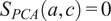 $ {S}_{PCA}\left(a,c\right)=0 $
. If both PCs are retained (
$ {S}_{PCA}\left(a,c\right)=0 $
. If both PCs are retained (
 $ Q=2 $
), the similarity factors are:
$ Q=2 $
), the similarity factors are:
 $ {S}_{PCA}\left(a,b\right)=0.87 $
,
$ {S}_{PCA}\left(a,b\right)=0.87 $
,
 $ {S}_{PCA}\left(a,c\right)=0.48 $
.
$ {S}_{PCA}\left(a,c\right)=0.48 $
.

Figure 9. The same bivariate normal distribution rotated by different angles with respect to the baseline, together with its principal components.
While
 $ {S}_{PCA} $
measures whether data matrices
$ {S}_{PCA} $
measures whether data matrices
 $ {\mathbf{X}}_1 $
and
$ {\mathbf{X}}_1 $
and
 $ {\mathbf{X}}_2 $
have similar correlation structures, it does not measure whether their mean value is comparable. Inside the combustion chamber, two spatial locations may have similar mixing trends over time between the multiple air and fuel streams, but the time-averaged value of the oxidizer and fuel streams mass fractions could be different. An example of two bivariate distributions having similar correlation structure but different mean point is illustrated Figure 10.
$ {\mathbf{X}}_2 $
have similar correlation structures, it does not measure whether their mean value is comparable. Inside the combustion chamber, two spatial locations may have similar mixing trends over time between the multiple air and fuel streams, but the time-averaged value of the oxidizer and fuel streams mass fractions could be different. An example of two bivariate distributions having similar correlation structure but different mean point is illustrated Figure 10.

Figure 10. Illustration of two bivariate distributions,
 $ {\mathbf{X}}_1 $
and
$ {\mathbf{X}}_1 $
and
 $ {\mathbf{X}}_2 $
, having a similar spatial orientation (similar PCs
$ {\mathbf{X}}_2 $
, having a similar spatial orientation (similar PCs
 $ {\mathbf{a}}_1 $
and
$ {\mathbf{a}}_1 $
and
 $ {\mathbf{a}}_2 $
) but located far apart, that is, their multivariate means, represented by vectors
$ {\mathbf{a}}_2 $
) but located far apart, that is, their multivariate means, represented by vectors
 $ {\overline{\mathbf{x}}}_1 $
and
$ {\overline{\mathbf{x}}}_1 $
and
 $ {\overline{\mathbf{x}}}_2 $
, are significantly different.
$ {\overline{\mathbf{x}}}_2 $
, are significantly different.
To account for the similarity in the multivariate mean, Singhal and Seborg (Reference Singhal and Seborg2005) propose an additional metric in their K-means clustering algorithm known as the distance similarity factor (
 $ {S}_{dist} $
) (Singhal and Seborg, Reference Singhal and Seborg2002), which is based on the Mahalanobis distance (
$ {S}_{dist} $
) (Singhal and Seborg, Reference Singhal and Seborg2002), which is based on the Mahalanobis distance (
 $ {D}_M $
) of a point from a distribution:
$ {D}_M $
) of a point from a distribution:
 $$ {D}_M=\sqrt{\left(\frac{{\overline{\mathbf{x}}}_2-{\overline{\mathbf{x}}}_1}{{\mathbf{d}}_1}\right)\;{\mathbf{S}}_1^{\star -1}\;{\left(\frac{{\overline{\mathbf{x}}}_2-{\overline{\mathbf{x}}}_1}{{\mathbf{d}}_1}\right)}^T}, $$
where
 $ {\overline{\mathbf{x}}}_1 $
and
$ {\overline{\mathbf{x}}}_1 $
and
 $ {\overline{\mathbf{x}}}_2 $
are the mean vectors of data matrices
$ {\overline{\mathbf{x}}}_2 $
are the mean vectors of data matrices
 $ {\mathbf{X}}_1 $
and
$ {\mathbf{X}}_1 $
and
 $ {\mathbf{X}}_2 $
, respectively, and
$ {\mathbf{X}}_2 $
, respectively, and
 $ {\mathbf{d}}_1 $
is the scaling vector of
$ {\mathbf{d}}_1 $
is the scaling vector of
 $ {\mathbf{X}}_1 $
(see Equation (8)).
$ {\mathbf{X}}_1 $
(see Equation (8)).
 $ {\mathbf{S}}_1^{\star -1} $
is the Moore–Penrose pseudo-inverse of the covariance of
$ {\mathbf{S}}_1^{\star -1} $
is the Moore–Penrose pseudo-inverse of the covariance of
 $ {\mathbf{X}}_1 $
(see Equation (5)). In Equation (10),
$ {\mathbf{X}}_1 $
(see Equation (5)). In Equation (10),
 $ {\mathbf{X}}_1 $
acts as the reference distribution against which the mean of
$ {\mathbf{X}}_1 $
acts as the reference distribution against which the mean of
 $ {\mathbf{X}}_2 $
is compared.
$ {\mathbf{X}}_2 $
is compared.
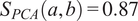
Employing the Mahalanobis distance takes into account the shape of the data distribution, which the Euclidean distance does not consider. For instance, imagine the distribution shown in Figure 11 represents a bivariate time series sampled at a reference spatial location of a simple combustion system consisting of only two streams (a single fuel inlet and a single oxidizer inlet). Points (1) and (3) represent the mean values at two different but nearby spatial locations. Although both points are the same Euclidean distance away from the mean of the reference distribution, point (1) operates, in an average sense, much closer to the distribution because it is a value that is typically observed at the reference location, whereas point (3) is not. While the example employed here is two-dimensional, this concept can be extended to any number of dimensions (any number of fuel and oxidizer streams).

Figure 11. Comparison of Mahalanobis and Euclidean distances in a bivariate distribution. The four points have the same Euclidean distance from the mean of the distribution at
 $ \left(0,0\right) $
, but points (3) and (4) have a much higher Mahalanobis distance.
$ \left(0,0\right) $
, but points (3) and (4) have a much higher Mahalanobis distance.
Because
 $ {D}_M $
can be arbitrarily large and it is convenient to have a similarity factor that is bounded between zero and unity, Singhal and Seborg (Reference Singhal and Seborg2002) suggest performing a monotonic mapping from
$ {D}_M $
can be arbitrarily large and it is convenient to have a similarity factor that is bounded between zero and unity, Singhal and Seborg (Reference Singhal and Seborg2002) suggest performing a monotonic mapping from
 $ {D}_M $
to
$ {D}_M $
to
 $ {S}_{dist} $
using the normal cumulative distribution function with zero mean:
$ {S}_{dist} $
using the normal cumulative distribution function with zero mean:
 $$ {S}_{dist}=2\hskip0.1em \left[1-\frac{1}{\sigma \sqrt{2\pi }}{\int}_{-\infty}^{D_M}\mathit{\exp}\left(-\frac{z^2}{2{\sigma}^2}\right) dz\right], $$
where
 $ {S}_{dist} $
is bounded between zero and unity and a variable standard deviation
$ {S}_{dist} $
is bounded between zero and unity and a variable standard deviation
 $ \sigma $
allows to control the rate of decay of
$ \sigma $
allows to control the rate of decay of
 $ {S}_{dist} $
with increasing
$ {S}_{dist} $
with increasing
 $ {D}_M $
, which is calculated from Equation (10).
$ {D}_M $
, which is calculated from Equation (10).
Based on the above discussion, two metrics can be employed to compare the mixing conditions of two spatial locations in a gas turbine combustor. The PCA similarity factor (Equation (9)) compares the correlation structure between the fuel and oxidizer streams at the two spatial locations. On the other hand, the distance similarity factor (Equation (11)) determines whether the mean operating conditions, in a time-average sense, of the two locations are similar. In the clustering algorithm, the two metrics can be combined into a single similarity factor
 $ S $
through a weighted sum:
$ S $
through a weighted sum:
 $$ S=\alpha {S}_{PCA}+\left(1-\alpha \right){S}_{dist}, $$
where
 $ \alpha $
, bounded between zero and unity, is the weight of the PCA similarity factor in the calculation of the combined metric. Through an appropriate choice of
$ \alpha $
, bounded between zero and unity, is the weight of the PCA similarity factor in the calculation of the combined metric. Through an appropriate choice of
 $ \alpha $
, higher relevance can be given to one similarity factor or the other. It is up to the user to choose the right value of
$ \alpha $
, higher relevance can be given to one similarity factor or the other. It is up to the user to choose the right value of
 $ \alpha $
depending on their application. Singhal and Seborg (Reference Singhal and Seborg2005) report good results with
$ \alpha $
depending on their application. Singhal and Seborg (Reference Singhal and Seborg2005) report good results with
 $ \alpha =0.67 $
, although this is highly dependent on the dataset the algorithm is applied to. In the application proposed in the present work, the main objective is to find spatial locations where the correlation between streams is similar, so that a single biplot can be used to visualize the mixing across a cluster of spatial locations. Therefore, values of
$ \alpha =0.67 $
, although this is highly dependent on the dataset the algorithm is applied to. In the application proposed in the present work, the main objective is to find spatial locations where the correlation between streams is similar, so that a single biplot can be used to visualize the mixing across a cluster of spatial locations. Therefore, values of
 $ \alpha >0.5 $
seem reasonable. The structure of the K-means clustering algorithm implemented in this work is summarized in Appendix, Section A.
$ \alpha >0.5 $
seem reasonable. The structure of the K-means clustering algorithm implemented in this work is summarized in Appendix, Section A.
3.6. Data sampling
In order to apply the statistical methodology described above, time series of the oxidizer passive scalars and the mixture fraction must be sampled across
 $ M $
spatial locations in regions of interest of the combustor during the LES calculation. The time series sampled at each spatial location are arranged into a tall matrix
$ M $
spatial locations in regions of interest of the combustor during the LES calculation. The time series sampled at each spatial location are arranged into a tall matrix
 $ \mathbf{X} $
of size
$ \mathbf{X} $
of size
 $ \left(N\times P\right) $
, where
$ \left(N\times P\right) $
, where
 $ N $
is the number of snapshots or temporal observations and
$ N $
is the number of snapshots or temporal observations and
 $ P $
is the number of passive scalars. In order to calculate statistically meaningful correlations between passive scalars, it is necessary to sample a sufficiently large number of statistically independent snapshots. As a general rule, the higher the statistical moment, the greater the fluctuation level of a random variable relative to its mean, and the greater its deviation from Gaussian behavior, the larger
$ P $
is the number of passive scalars. In order to calculate statistically meaningful correlations between passive scalars, it is necessary to sample a sufficiently large number of statistically independent snapshots. As a general rule, the higher the statistical moment, the greater the fluctuation level of a random variable relative to its mean, and the greater its deviation from Gaussian behavior, the larger
 $ N $
needs to be to achieve a sufficiently high statistical accuracy (Pope, Reference Pope2000).
$ N $
needs to be to achieve a sufficiently high statistical accuracy (Pope, Reference Pope2000).
Figure 12 shows the convergence of the correlation coefficients of the mixture fraction with the oxidizer passive scalars at two locations of the experimental test rig (see Section 2.2) as a function of sampling time. The two spatial locations have significantly different turbulence intensity, given by
 $ I={u}_{rms}/\overline{u} $
, where
$ I={u}_{rms}/\overline{u} $
, where
 $ {u}_{rms} $
and
$ {u}_{rms} $
and
 $ \overline{u} $
are the root-mean-square and mean velocities, respectively. At location 1, convergence is reached relatively quickly. However, at location 2, positioned close to the IRZ, it takes approximately 30
$ \overline{u} $
are the root-mean-square and mean velocities, respectively. At location 1, convergence is reached relatively quickly. However, at location 2, positioned close to the IRZ, it takes approximately 30
 $ ms $
to reach convergence, three times longer than the estimated flow-through time (the average time it takes a fluid particle to cross the combustor from inlet to outlet).
$ ms $
to reach convergence, three times longer than the estimated flow-through time (the average time it takes a fluid particle to cross the combustor from inlet to outlet).

Figure 12. Statistical convergence of the correlation coefficients of the mixture fraction with the oxidizer passive scalars at two spatial locations of the experimental test rig with different turbulence intensity (
 $ I $
).
$ I $
).
4. Results
4.1. Choosing the number of clusters
The key hyperparameter when applying the K-means clustering algorithm is the choice of number of clusters (
 $ K $
). In this work, following the discussion in Section 3.5, a cluster may be seen as a “mixing region”, where the combustor spatial locations belonging to the same cluster have similar mixing characteristics (as described by the relationship between the fuel and oxidizer stream tracers, sampled over time and arranged into a tall matrix
$ K $
). In this work, following the discussion in Section 3.5, a cluster may be seen as a “mixing region”, where the combustor spatial locations belonging to the same cluster have similar mixing characteristics (as described by the relationship between the fuel and oxidizer stream tracers, sampled over time and arranged into a tall matrix
 $ \mathbf{X} $
).
$ \mathbf{X} $
).
To choose an appropriate value of
 $ K $
, Singhal and Seborg (Reference Singhal and Seborg2005) define a cost function based on the dissimilarity factor:
$ K $
, Singhal and Seborg (Reference Singhal and Seborg2005) define a cost function based on the dissimilarity factor:
 $$ {d}_{i,m}=1-{S}_{i,m}, $$
where
 $ {S}_{i,m} $
is the similarity factor (Equation (12)) between the
$ {S}_{i,m} $
is the similarity factor (Equation (12)) between the
 $ {m}^{th} $
data instance (in our case, the
$ {m}^{th} $
data instance (in our case, the
 $ {\mathbf{X}}_m $
matrix at the
$ {\mathbf{X}}_m $
matrix at the
 $ {m}^{th} $
spatial location) and the
$ {m}^{th} $
spatial location) and the
 $ {i}^{th} $
cluster
$ {i}^{th} $
cluster
 $ {\mathbf{C}}_i $
(Equation (16)) it belongs to, and
$ {\mathbf{C}}_i $
(Equation (16)) it belongs to, and
 $ {d}_{i,m} $
is the corresponding dissimilarity factor. The cost function is then defined as an average of
$ {d}_{i,m} $
is the corresponding dissimilarity factor. The cost function is then defined as an average of
 $ {d}_{i,m} $
across all clusters:
$ {d}_{i,m} $
across all clusters:
 $$ J(K)=\frac{1}{M}\sum \limits_{i=1}^K\sum \limits_{{\mathbf{X}}_m\in {\mathbf{C}}_i}{d}_{i,m}, $$
where
 $ M $
is the total number of data instances (spatial locations) and
$ M $
is the total number of data instances (spatial locations) and
 $ K $
is the number of clusters. The clustering algorithm can then be run with an increasing number of clusters and the change of
$ K $
is the number of clusters. The clustering algorithm can then be run with an increasing number of clusters and the change of
 $ J(K) $
with
$ J(K) $
with
 $ K $
can be monitored. A similar approach was followed by D’Alessio et al. (Reference D’Alessio, Attili, Cuoci, Pitsch, Parente, Pitsch and Attili2020) in their application of local PCA for the thermochemical analysis of turbulent reacting jets: plotting the reconstruction error (their choice of cost function) as a function of the number of clusters and identifying the location where the curve starts to asymptote.
$ K $
can be monitored. A similar approach was followed by D’Alessio et al. (Reference D’Alessio, Attili, Cuoci, Pitsch, Parente, Pitsch and Attili2020) in their application of local PCA for the thermochemical analysis of turbulent reacting jets: plotting the reconstruction error (their choice of cost function) as a function of the number of clusters and identifying the location where the curve starts to asymptote.
Figure 13 shows
 $ J(K) $
as a function of the number of clusters
$ J(K) $
as a function of the number of clusters
 $ K $
for data sampled from the experimental test rig simulation (see Section 2.2). As expected,
$ K $
for data sampled from the experimental test rig simulation (see Section 2.2). As expected,
 $ J(K) $
decreases as
$ J(K) $
decreases as
 $ K $
is increased because the clusters become smaller and internally more homogeneous. We would also expect the curve to eventually asymptote if
$ K $
is increased because the clusters become smaller and internally more homogeneous. We would also expect the curve to eventually asymptote if
 $ K $
was increased further. In the context of this work, the main objective of spatial clustering is to reduce the large spatial dimensionality of the mixing problem so that a single biplot (Section 3.4) can be employed to visually examine the fuel–air mixing patterns across a region of the combustor. Increasing
$ K $
was increased further. In the context of this work, the main objective of spatial clustering is to reduce the large spatial dimensionality of the mixing problem so that a single biplot (Section 3.4) can be employed to visually examine the fuel–air mixing patterns across a region of the combustor. Increasing
 $ K $
will provide a more optimized decomposition of the dataset, but will also increase the number of biplots that need to be analyzed.
$ K $
will provide a more optimized decomposition of the dataset, but will also increase the number of biplots that need to be analyzed.

Figure 13. Cost function
 $ J(K) $
as a function of the number of clusters
$ J(K) $
as a function of the number of clusters
 $ K $
using (i) all spatial locations and (ii) half of the spatial locations (randomly sampled) across the mid-plane of the experimental test rig.
$ K $
using (i) all spatial locations and (ii) half of the spatial locations (randomly sampled) across the mid-plane of the experimental test rig.
4.2. Robustness to initialization
The K-means clustering algorithm can converge to a solution that is a local (nonglobal) minimum. This means that the final solution may be sensitive to the user-provided initialization. Ideally, the converged solution should be reasonably independent from the initial guess provided by the user, and the algorithm should identify the same mixing regions in the combustor regardless of the initialization.
Figure 14 shows converged solutions of the clustering algorithm for the mid-plane of the experimental test rig (see Figure 2 for reference) for two different initializations. The passive scalar time series were mean-centered and Pareto-scaled in a preprocessing step (see Section 3.3), thus giving more relevance in the low-order PCA models to the streams with high variance. In this case, the algorithm was run with
 $ \alpha =1 $
(see Equation (12)); that is, only similarity in the passive scalar correlation structure was considered. The zero mean axial velocity level is also shown in Figure 14 to help identify regions of flow recirculation. As illustrated, although the two initializations are completely dissimilar, the converged solutions are very close. Additionally, the converged solutions agree well with the flow physics inside a gas turbine combustor. For instance, clusters 1 and 2 in Figure 14b are dominated by the injector flow and the transition from cluster 1 to cluster 2 is dominated by the completion of spray evaporation as well as the completion of the mixing between the IS and OS streams. Cluster 9 is clearly dominated by the FC flow, designed to remain attached to the combustor wall and prevent it from overheating. The reader is reminded that K-means clustering is a type of unsupervised machine learning, and that the algorithm has no information about the spatial distribution of the data instances.
$ \alpha =1 $
(see Equation (12)); that is, only similarity in the passive scalar correlation structure was considered. The zero mean axial velocity level is also shown in Figure 14 to help identify regions of flow recirculation. As illustrated, although the two initializations are completely dissimilar, the converged solutions are very close. Additionally, the converged solutions agree well with the flow physics inside a gas turbine combustor. For instance, clusters 1 and 2 in Figure 14b are dominated by the injector flow and the transition from cluster 1 to cluster 2 is dominated by the completion of spray evaporation as well as the completion of the mixing between the IS and OS streams. Cluster 9 is clearly dominated by the FC flow, designed to remain attached to the combustor wall and prevent it from overheating. The reader is reminded that K-means clustering is a type of unsupervised machine learning, and that the algorithm has no information about the spatial distribution of the data instances.

Figure 14. Converged solutions of K-means clustering across the mid-plane of the experimental rig for two different algorithm initializations, with
 $ K=16 $
and
$ K=16 $
and
 $ {S}_{PCA} $
weighting
$ {S}_{PCA} $
weighting
 $ \alpha =1 $
. Every color represents a different cluster. The black isoline is the zero mean axial velocity level (
$ \alpha =1 $
. Every color represents a different cluster. The black isoline is the zero mean axial velocity level (
 $ {\overline{u}}_x=0 $
). The coordinates have been normalized by one injector diameter
$ {\overline{u}}_x=0 $
). The coordinates have been normalized by one injector diameter
 $ D $
.
$ D $
.
Figure 15 illustrates the biplots of clusters 2 and 7 shown in Figure 14b, as well as the biplots of the median spatial location of each cluster. The biplots are plotted in the space spanned by the first two PCs (which represent at least 80% of the total variance in all cases), following the strategy described in Section 3.4 (coloring temporal observations according to their instantaneous mixture fraction value). Although some small differences exist, the biplots of the clusters and of their respective median points are alike, indicating the similarity in their covariance structure. This proves the usefulness of the proposed implementation of the K-means clustering algorithm: a cluster consists of spatial locations with similar mixing characteristics (covariance structure between stream tracers), so that a single biplot is an accurate representation of the mixing taking place across all the spatial locations that belong to the cluster. Figure 15a,c show that, despite the physical proximity of the DS, IS, and OS inlets (see Figure 2), the DS flow struggles to complete its mixing with the IS and OS flows, which are the main fuel carriers (DS is perpendicular to IS and OS, indicating lack of linear correlation). This is the case even at cluster 7, which is located more than 1.5 injector diameters downstream of the injector outlet. Figure 15a,c also indicate that the FC flow plays a relevant role leaning the fuel–air mixture in both clusters, as it has a large magnitude vector which points in the direction of the fuel-lean cloud of observations.

Figure 15. Biplots of clusters 2 and 7 and of their corresponding median point. The cluster numbering follows Figure 14b. The variance explained by each principal component is indicated in brackets. The data were Pareto-scaled prior to PCA.
4.3. Solution convergence
One approach to monitor the convergence of the K-means clustering algorithm is to plot the cost function
 $ J(K) $
(Equation (14)) as a function of the number of iterations. This is illustrated in Figure 16a for the converged solution shown in Figure 14b with
$ J(K) $
(Equation (14)) as a function of the number of iterations. This is illustrated in Figure 16a for the converged solution shown in Figure 14b with
 $ K=16 $
clusters. The algorithm is able to achieve convergence after approximately 10 iterations following the initialization of Figure 14a, on a tabletop workstation in less than 5 minutes. This particular dataset consisted of
$ K=16 $
clusters. The algorithm is able to achieve convergence after approximately 10 iterations following the initialization of Figure 14a, on a tabletop workstation in less than 5 minutes. This particular dataset consisted of
 $ 9000 $
sampled spatial locations, with a matrix
$ 9000 $
sampled spatial locations, with a matrix
 $ \mathbf{X} $
of size (
$ \mathbf{X} $
of size (
 $ 2000\times 8 $
) at each spatial location.
$ 2000\times 8 $
) at each spatial location.

Figure 16. The cost function
 $ J(K) $
as a function of the number of algorithm iterations and the within-cluster dissimilarity
$ J(K) $
as a function of the number of algorithm iterations and the within-cluster dissimilarity
 $ {J}_i $
at initialization and at convergence.
$ {J}_i $
at initialization and at convergence.
To quantify the homogeneity of a given cluster at convergence, one can calculate the average within-cluster dissimilarity for the
 $ {i}^{th} $
cluster as:
$ {i}^{th} $
cluster as:
 $$ {J}_i=\frac{1}{M_i}\sum \limits_{{\mathbf{X}}_m\in {\mathbf{C}}_i}{d}_{i,m}, $$
where
 $ {d}_{i,m} $
is the dissimilarity factor (Equation (13)) between the
$ {d}_{i,m} $
is the dissimilarity factor (Equation (13)) between the
 $ {m}^{th} $
data instance
$ {m}^{th} $
data instance
 $ {\mathbf{X}}_m $
and the
$ {\mathbf{X}}_m $
and the
 $ {i}^{th} $
cluster
$ {i}^{th} $
cluster
 $ {\mathbf{C}}_i $
, and
$ {\mathbf{C}}_i $
, and
 $ {M}_i $
is the number of data instances in the
$ {M}_i $
is the number of data instances in the
 $ {i}^{th} $
cluster. Figure 16b shows the average within-cluster dissimilarity across all 16 clusters at initialization and at convergence. As illustrated, all clusters are considerably inhomogeneous at initialization, as would be expected.
$ {i}^{th} $
cluster. Figure 16b shows the average within-cluster dissimilarity across all 16 clusters at initialization and at convergence. As illustrated, all clusters are considerably inhomogeneous at initialization, as would be expected.
 $ {J}_i $
drops for all clusters as the algorithm iterates and the clusters are filled with spatial locations with similar correlation structures between stream tracers. At convergence, clusters 1 and 6 are considerably inhomogeneous relative to the other clusters. These correspond to the region just downstream of the injector exit plane and the mixing zone along the chamber back wall (see Figure 14b). The high value of
$ {J}_i $
drops for all clusters as the algorithm iterates and the clusters are filled with spatial locations with similar correlation structures between stream tracers. At convergence, clusters 1 and 6 are considerably inhomogeneous relative to the other clusters. These correspond to the region just downstream of the injector exit plane and the mixing zone along the chamber back wall (see Figure 14b). The high value of
 $ {J}_i $
for cluster 1 may be explained by the evaporating spray, the incomplete mixing between the injector swirler flows and the gaseous fuel, and the presence of strong flow recirculation. In the case of cluster 6, in addition to flow recirculation, the mixture inhomogeneity may be explained by the shear-driven mixing layer between the DS flow, the HSC and the FC flows (see Figure 2 for reference). All of these processes lead to strong spatial gradients in the mixture fraction and oxidizer passive scalar fields, resulting in a comparatively inhomogeneous cluster relative to the other clusters.
$ {J}_i $
for cluster 1 may be explained by the evaporating spray, the incomplete mixing between the injector swirler flows and the gaseous fuel, and the presence of strong flow recirculation. In the case of cluster 6, in addition to flow recirculation, the mixture inhomogeneity may be explained by the shear-driven mixing layer between the DS flow, the HSC and the FC flows (see Figure 2 for reference). All of these processes lead to strong spatial gradients in the mixture fraction and oxidizer passive scalar fields, resulting in a comparatively inhomogeneous cluster relative to the other clusters.
4.4. Similarity in mean operating point
The results presented in Figure 14 correspond to a
 $ {S}_{PCA} $
weighting factor of
$ {S}_{PCA} $
weighting factor of
 $ \alpha =1 $
(Equation (12)). In other words, the similarity in the mean operating point between spatial locations was not taken into account in the K-means clustering algorithm. Figure 17 shows the converged solutions of the experimental test rig mid-plane with
$ \alpha =1 $
(Equation (12)). In other words, the similarity in the mean operating point between spatial locations was not taken into account in the K-means clustering algorithm. Figure 17 shows the converged solutions of the experimental test rig mid-plane with
 $ \alpha =1 $
and
$ \alpha =1 $
and
 $ \alpha =0.67 $
. Both iterations of the algorithm were started from the same initialization and run until converged. A value of
$ \alpha =0.67 $
. Both iterations of the algorithm were started from the same initialization and run until converged. A value of
 $ \alpha =0.67 $
gives the PCA similarity factor a weight of
$ \alpha =0.67 $
gives the PCA similarity factor a weight of
 $ 2/3 $
in the clustering algorithm cost function, while the distance similarity factor, which measures the similarity in the multivariate mean of the oxidizer passive scalars and mixture fraction time series, is given a weight of
$ 2/3 $
in the clustering algorithm cost function, while the distance similarity factor, which measures the similarity in the multivariate mean of the oxidizer passive scalars and mixture fraction time series, is given a weight of
 $ 1/3 $
.
$ 1/3 $
.

Figure 17. Converged solutions of the experimental rig data with
 $ K=16 $
clusters with two different
$ K=16 $
clusters with two different
 $ {S}_{PCA} $
weighting factors (
$ {S}_{PCA} $
weighting factors (
 $ \alpha $
). The black isoline is the zero mean axial velocity level (
$ \alpha $
). The black isoline is the zero mean axial velocity level (
 $ {\overline{u}}_x=0 $
). The coordinates have been normalized by one injector diameter
$ {\overline{u}}_x=0 $
). The coordinates have been normalized by one injector diameter
 $ D $
.
$ D $
.
As illustrated in Figure 17, although the identified patterns are similar, incorporating
 $ {S}_{dist} $
in the K-means clustering algorithm has an important influence on the solution. For instance, cluster 1 in Figure 17b extends radially inward into the fuel injector exit plane, compared to cluster 6 in Figure 17a. This may be explained by the dominance of the DS flow mass fraction across this cluster (see Figure 2 for reference). Due to the steep metal angle of the injector assembly at the exit plane, the DS flow undergoes a sudden outward radial expansion once it exits the injector, and tends to remain attached to the combustor back wall, increasing its mass fraction across cluster 1 in Figure 17b. While the correlation structure between stream tracers is likely to be more homogeneous within clusters 1 and 6 in Figure 17a,
$ {S}_{dist} $
in the K-means clustering algorithm has an important influence on the solution. For instance, cluster 1 in Figure 17b extends radially inward into the fuel injector exit plane, compared to cluster 6 in Figure 17a. This may be explained by the dominance of the DS flow mass fraction across this cluster (see Figure 2 for reference). Due to the steep metal angle of the injector assembly at the exit plane, the DS flow undergoes a sudden outward radial expansion once it exits the injector, and tends to remain attached to the combustor back wall, increasing its mass fraction across cluster 1 in Figure 17b. While the correlation structure between stream tracers is likely to be more homogeneous within clusters 1 and 6 in Figure 17a,
 $ {S}_{PCA} $
alone (
$ {S}_{PCA} $
alone (
 $ \alpha $
= 1) cannot capture the dominance of the DS flow across cluster 1 of Figure 17b in terms of its mean mass fraction. A similar situation is encountered across cluster 10 in Figure 17b, whose composition is dominated by the FC flow mass fraction, which is designed to stick to combustor wall to prevent damage from overheating. With
$ \alpha $
= 1) cannot capture the dominance of the DS flow across cluster 1 of Figure 17b in terms of its mean mass fraction. A similar situation is encountered across cluster 10 in Figure 17b, whose composition is dominated by the FC flow mass fraction, which is designed to stick to combustor wall to prevent damage from overheating. With
 $ \alpha =1 $
, this region of the combustor is split into multiple clusters in the vicinity of the FC inlet due to the somewhat different correlation structures that result from the shear-driven mixing with the HSC and DS flows. However, because the mean mass fraction is nevertheless dominated by the FC flow, the clustering algorithm identifies this region as a unique cluster when
$ \alpha =1 $
, this region of the combustor is split into multiple clusters in the vicinity of the FC inlet due to the somewhat different correlation structures that result from the shear-driven mixing with the HSC and DS flows. However, because the mean mass fraction is nevertheless dominated by the FC flow, the clustering algorithm identifies this region as a unique cluster when
 $ \alpha =0.67 $
. Another interesting difference between
$ \alpha =0.67 $
. Another interesting difference between
 $ \alpha =1 $
and
$ \alpha =1 $
and
 $ \alpha =0.67 $
happens at cluster 15 of Figure 17a, which is split into clusters 12 and 15 in Figure 17b. Analysis of the time-averaged passive scalars across clusters 12 and 15 of Figure 17b shows that the mass fraction of the dilution port flow emanating from the top wall (at
$ \alpha =0.67 $
happens at cluster 15 of Figure 17a, which is split into clusters 12 and 15 in Figure 17b. Analysis of the time-averaged passive scalars across clusters 12 and 15 of Figure 17b shows that the mass fraction of the dilution port flow emanating from the top wall (at
 $ x/D\approx 2.1 $
,
$ x/D\approx 2.1 $
,
 $ z/D=+1.3 $
) is much higher in cluster 15 than in cluster 12. This may be explained by the proximity of cluster 15 to the impingement point between the top and bottom dilution port jets, close to the chamber centerline at
$ z/D=+1.3 $
) is much higher in cluster 15 than in cluster 12. This may be explained by the proximity of cluster 15 to the impingement point between the top and bottom dilution port jets, close to the chamber centerline at
 $ z/D=0 $
.
$ z/D=0 $
.
4.5. Analysis of the detailed single-sector combustor
The previous sections looked at the application of the PCA and K-means clustering methodology to the simulation results of the experimental test rig operating at low power. This section will discuss the application of the methodology to the detailed single-sector combustor operating at high power, which is a more realistic representation of the aeroengine combustor flow field and operating conditions (see Section 2.2).
Figure 18 shows the converged solution of the clustering algorithm applied to the combustor mid-plane. This dataset consists of approximately 10,000 uniformly distributed spatial locations, with a matrix of 10 passive scalars and approximately 150 temporal samples at each spatial location. Algorithm convergence was achieved in approximately 5 minutes on a desktop workstation. The
 $ {S}_{PCA} $
weighting factor
$ {S}_{PCA} $
weighting factor
 $ \alpha $
(Equation (12)) was set to 0.67, and the passive scalars were mean-centered and Pareto-scaled in a preprocessing step. Unlike the experimental test rig case, which is circumferentially symmetrical about the injector centerline, the inner and outer wall FC flows in the single-sector combustor are tagged by two separate passive scalars. Following the analysis described in Section 4.1, the number of clusters was chosen to be
$ \alpha $
(Equation (12)) was set to 0.67, and the passive scalars were mean-centered and Pareto-scaled in a preprocessing step. Unlike the experimental test rig case, which is circumferentially symmetrical about the injector centerline, the inner and outer wall FC flows in the single-sector combustor are tagged by two separate passive scalars. Following the analysis described in Section 4.1, the number of clusters was chosen to be
 $ K=20 $
, which gives a good balance between the discretization of the dataset and the total number of clusters to be visually analyzed.
$ K=20 $
, which gives a good balance between the discretization of the dataset and the total number of clusters to be visually analyzed.

Figure 18. Mid-plane of the single-sector combustor showing all oxidizer inlets into the chamber and the converged solution of the K-means clustering algorithm with 20 clusters. The white isoline is the zero mean axial velocity level (
 $ {\overline{u}}_x=0 $
). The coordinates have been normalized by one injector diameter
$ {\overline{u}}_x=0 $
). The coordinates have been normalized by one injector diameter
 $ D $
. The internal components of the fuel injector have been concealed due to commercial confidentiality.
$ D $
. The internal components of the fuel injector have been concealed due to commercial confidentiality.
Similar to the analysis of the experimental test rig in the previous sections, the converged solution of Figure 18b shows considerable symmetry in the cluster arrangement about the injector centerline, with major discrepancies between the top and bottom halves resulting from the labeling of the inner and outer FC flows, as well as the inner and outer port flows, with separate passive scalars. Cluster 4 is very close to the fuel prefilmer, where the liquid fuel is injected into the chamber, and this cluster is therefore dominated by the liquid fuel spray, which has not yet completed evaporation.
Figure 19 shows the biplots across clusters 2, 3, and 8 of Figure 18b. The biplots were produced following the strategy described in Section 3.4, that is, performing PCA on the Pareto-scaled oxidizer streams and using the mixture fraction to color the observations projected onto the space of the first two PCs. Cluster 2 is clearly dominated by the IS, the OS, and the DS flows. The IS is pointing in the direction of the fuel-rich data cloud, indicating that a significant amount of fuel has evaporated from the liquid spray and has had time to mix with the IS flow by the time the fuel reaches cluster 2. Figure 19a also shows that the IS and the DS are strongly anticorrelated, indicating that they compete against each other over time in the mixing across cluster 2. The OS, on the other hand, is not strongly linearly correlated with either the IS or the DS, indicating that some amount of mixing may have occurred (especially with the IS), but that this mixing is not yet complete, which appears reasonable given the proximity of cluster 2 to the injector outlet. Figure 19b shows that the correlation between the IS and the OS flows across cluster 8 is considerably increased compared to cluster 2, indicating a relatively high degree of mixing between the two streams by the time they reach this cluster. The DS is still the dominant oxidizer contributing toward leaning the mixture, but the Inner Port (IP) and Outer Port (OP) flows also have a non-negligible role. Figure 19c shows that in cluster 3, the OS and IS are strongly positively correlated with each other and with the fuel mixture fraction (i.e., they are the main fuel carriers into cluster 3). Unlike in clusters 2 and 8, the DS is no longer strongly anticorrelated with the IS, indicating that some degree of mixing between the two streams has taken place. Due to the proximity of cluster 3 to their respective outlets, the HSC and locating ring cooling (LRC) streams have a relevant role in the mixing across this cluster (see Figure 19d). They have large magnitude vectors that clearly point in the direction of the fuel-lean data cloud, and are strongly anticorrelated with the IS and OS, indicating they are the main oxidizers contributing toward leaning the mixture across this cluster.

Figure 19. Biplots of clusters 2, 3, and 8 of the single-sector combustor mid-plane. The cluster numbering follows Figure 18b. The percentage of total variance explained by each PC, as well as the mean time-averaged mixture fraction across each cluster, is indicated in brackets.
The above discussion can be linked to the time-averaged results of the flow field illustrated in Figure 20. The reader is reminded that streamlines are everywhere tangential to the local velocity vector. The mean velocity field shown in Figure 20a is typical of a gas turbine combustor: vortex breakdown occurs within one injector diameter downstream of the injector exit plane, leading to the formation of a large IRZ. An outer recirculation zone (ORZ) is also formed in the vicinity of the chamber back wall. The fuel injector airflow forms a cone-shaped stream into the chamber that undergoes a radial expansion between the IRZ and ORZ. Figure 20b shows the time-averaged liquid mixture fraction in the vicinity of the fuel injector, where the liquid mixture fraction is defined as the local ratio of liquid-phase mass flux to the total mass flux (liquid- and gaseous-phase). As illustrated, the liquid fuel evaporates quickly after injection, and the core of the fuel spray is aligned with the streamlines emanating from the IS and OS. Comparatively, there is little interaction between the flow emanating from the DS and the fuel spray in the vicinity of the fuel injector, suggesting low mixing rates between the two streams. Figure 20c shows the time-averaged gaseous mixture fraction across the combustor mid-plane, and indicates that the highest concentration of gaseous fuel occurs just after the liquid spray completes its evaporation, on the edge of the IRZ. After evaporation, the gaseous fuel is carried downstream primarily by the IS and OS flows. This is corroborated by the proximity of the mixture fraction isolines in the vicinity of the evaporating spray in Figure 20d, which indicates strong mixing rates of the fuel with the IS and OS flows, while the mixing between the fuel stream and the DS flow takes place further downstream. These observations agree well with the analysis of the biplots of Figure 19.

Figure 20. Time-averaged profiles of velocity, liquid, and gaseous mixture fraction across the mid-plane of the single-sector combustor. The coordinates have been normalized by one injector diameter
 $ D $
. The internal components of the fuel injector have been concealed due to commercial confidentiality.
$ D $
. The internal components of the fuel injector have been concealed due to commercial confidentiality.
Finally, Figure 21 shows the converged solution of the clustering algorithm (with a weighting factor
 $ \alpha =0.67 $
) applied to a dataset consisting of two perpendicular planes of the single-sector combustor, illustrating that the algorithm can be applied to any spatial distribution. With the additional plane, the dataset becomes considerably larger: a total of approximately 19,000 spatial locations. Due to the increased dataset size, the number of clusters was increased to
$ \alpha =0.67 $
) applied to a dataset consisting of two perpendicular planes of the single-sector combustor, illustrating that the algorithm can be applied to any spatial distribution. With the additional plane, the dataset becomes considerably larger: a total of approximately 19,000 spatial locations. Due to the increased dataset size, the number of clusters was increased to
 $ K=22 $
. In Figure 21b, it is interesting to point out that cluster 7 matches the shape of the zero-axial-velocity line, and the continuity of cluster 13 across the side walls due to the imposed periodic boundary condition in the LES calculation.
$ K=22 $
. In Figure 21b, it is interesting to point out that cluster 7 matches the shape of the zero-axial-velocity line, and the continuity of cluster 13 across the side walls due to the imposed periodic boundary condition in the LES calculation.

Figure 21. Converged solution of the clustering algorithm with
 $ K=22 $
clusters for a dataset of the single-sector combustor consisting of two perpendicular planes. The dashed black line indicates the location of the perpendicular plane. The white isoline is the zero mean axial velocity level (
$ K=22 $
clusters for a dataset of the single-sector combustor consisting of two perpendicular planes. The dashed black line indicates the location of the perpendicular plane. The white isoline is the zero mean axial velocity level (
 $ {\overline{u}}_x=0 $
). The coordinates have been normalized by one injector diameter
$ {\overline{u}}_x=0 $
). The coordinates have been normalized by one injector diameter
 $ D $
. The internal components of the fuel injector have been concealed due to commercial confidentiality.
$ D $
. The internal components of the fuel injector have been concealed due to commercial confidentiality.
5. Conclusion
Modern gas turbine combustors consist of a large number of air inflows whose influence on local fuel–air mixing is hard to quantify. This work introduces a computationally efficient statistical method for analyzing local fuel–air mixing in realistic gas turbine combustors by post-processing time-resolved data from reacting-flow LES with tagged passive scalars for stream tracing. By applying PCA to the time series of these scalars at each spatial location, we construct low-order models that capture the dominant mixing trends and enable visual interpretation via biplots. A custom clustering approach, combining PCA similarity with the Mahalanobis distance, then groups spatial regions with similar mixing characteristics in an unsupervised fashion. The resulting clusters align well with known flow features inside gas turbine combustors, such as recirculating regions and shear layers, providing a compact and interpretable summary of complex multi-stream mixing. This methodology enhances engineers’ ability to diagnose and visualize complex fuel–air mixing patterns in modern combustors, potentially informing design decisions aimed at improving combustion efficiency and reducing emissions. Future work will explore the integration of nonlinear dimensionality reduction methods, balancing improved accuracy with the need for interpretability and computational practicality.
Acknowledgments
The authors would like to acknowledge the support of Rolls-Royce plc. and the National Centre for Combustion and Aerothermal Technology at Loughborough University.
Author contribution
Conceptualization: D.S.J.; A.D.W.; J.F.C. Data Curation: D.S.J. Formal analysis: D.S.J. Investigation: D.S.J. Methodology: D.S.J. Software: D.S.J. Validation: D.S.J. Visualization: D.S.J. Funding Acquisition: A.D.W.; J.F.C. Project Administration: A.D.W; J.F.C. Supervision: A.D.W; J.F.C. Writing - original draft: D.S.J. Writing - review & editing: A.D.W.; J.F.C. All authors approved the final submitted draft.
Data availability statement
The LES data and software used to generate the results presented in this article are proprietary and subject to confidentiality restrictions, and therefore cannot be publicly shared.
Funding statement
This research was funded in part by the EPSRC Centre for Doctoral Training in Future Propulsion and Power, Training Grant Reference: EP/S023003/1.
Competing interests
The authors declare none.
Ethical standard
The research meets all ethical guidelines, including adherence to the legal requirements of the study country.
A. Clustering Algorithm
This section summarizes the structure of the modified K-means clustering algorithm implemented in this work using MATLAB. It is based on the algorithm proposed by Singhal and Seborg (Reference Singhal and Seborg2005).
Given
 $ M $
matrices
$ M $
matrices
 $ {\mathbf{X}}_m $
of shape
$ {\mathbf{X}}_m $
of shape
 $ \left(N\times P\right) $
, where
$ \left(N\times P\right) $
, where
 $ N $
is the number of flow snapshots over time and
$ N $
is the number of flow snapshots over time and
 $ P $
is the number of passive scalars, sampled at
$ P $
is the number of passive scalars, sampled at
 $ M $
different spatial locations from a LES calculation, the algorithm proceeds as follows:
$ M $
different spatial locations from a LES calculation, the algorithm proceeds as follows:
-
1. Perform data preprocessing of each
$ {\mathbf{X}}_m $
matrix (mean centering and scaling). -
2. Perform a PCA decomposition of each
$ {\mathbf{X}}_m $
matrix. Store the eigenvectors and corresponding eigenvalues. -
3. Initialize the algorithm by splitting the dataset into
$ K $
initial clusters or seeds, where
$ K $
is a hyperparameter. It is well known that the K-means clustering algorithm risks converging to a local (nonglobal) minimum (Brunton and Kutz, Reference Brunton and Kutz2019). In other words, the final solution can be influenced by the initial allocation, so it is worth testing different initializations. Each of the
$ K $
clusters
$ {\mathbf{C}}_i $
is built by vertically concatenating its members
$ {\mathbf{X}}_m^{(i)} $
into a single tall and skinny matrix:


 $$ {\mathbf{C}}_i={\left[{\left({\mathbf{X}}_1^{(i)}\right)}^T\hskip0.1em {\left({\mathbf{X}}_2^{(i)}\right)}^T\dots {\left({\mathbf{X}}_{M_i}^{(i)}\right)}^T\right]}^T, $$
where
 $ 1\le i\le K $
and
$ 1\le i\le K $
and
 $ {\sum}_{i=1}^K{M}_i=M $
.
$ {\sum}_{i=1}^K{M}_i=M $
.
 $ {\mathbf{C}}_i $
acts as a prototype for the
$ {\mathbf{C}}_i $
acts as a prototype for the
 $ {i}^{th} $
cluster, so that a PCA model of
$ {i}^{th} $
cluster, so that a PCA model of
 $ {\mathbf{C}}_i $
for the calculation of
$ {\mathbf{C}}_i $
for the calculation of
 $ {S}_{PCA} $
(Equation (9)), or its covariance pseudo-inverse and mean vector for the calculation of
$ {S}_{PCA} $
(Equation (9)), or its covariance pseudo-inverse and mean vector for the calculation of
 $ {S}_{dist} $
(Equation (11)), are representative of the
$ {S}_{dist} $
(Equation (11)), are representative of the
 $ {i}^{th} $
cluster centroid.
$ {i}^{th} $
cluster centroid.
-
4. Calculate the dissimilarity
$ {d}_{i,m} $
between every matrix
$ {\mathbf{X}}_m $
and each cluster
$ {\mathbf{C}}_i $
(Equation (13)). -
5. Assign
$ {\mathbf{X}}_m $
to the cluster to which it is least dissimilar, that is, to the cluster with the lowest
$ {d}_{i,m} $
. Repeat the process for all
$ M $
matrices. -
6. Calculate the within-cluster dissimilarity
$ {J}_i $
for each of the
$ K $
clusters (Equation (15)) and the global dissimilarity
$ J(K) $
for all
$ M $
matrices across all
$ K $
clusters (Equation (14)). -
7. Evaluate the solution convergence. Has
$ J(K) $
changed beyond a user-specified tolerance with respect to the previous algorithm iteration? And, is the current iteration below the user-specified maximum number of iterations? If the answer is yes, return to Step 4 and continue iterating. If the answer is no, end the algorithm.


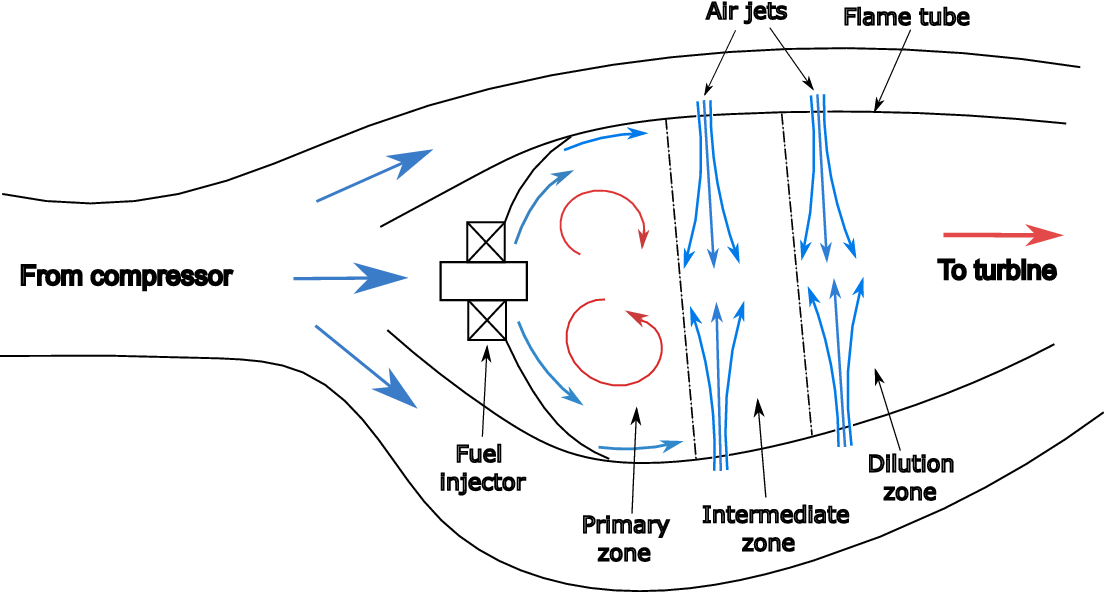


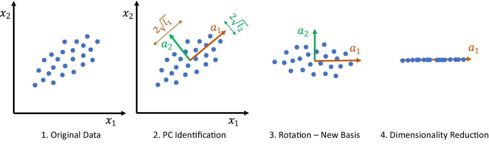


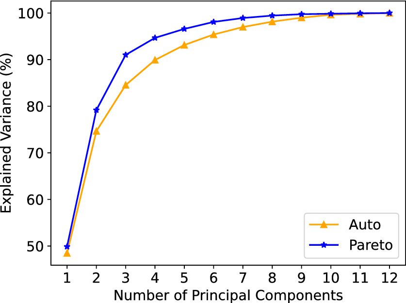
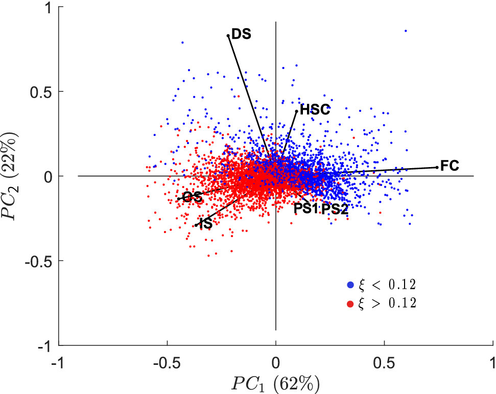

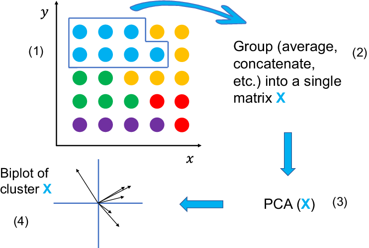

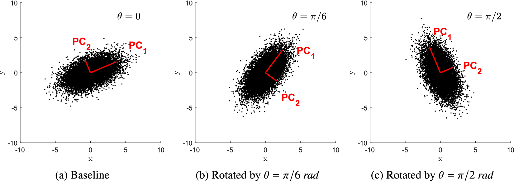
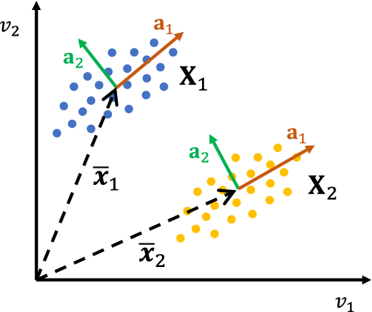


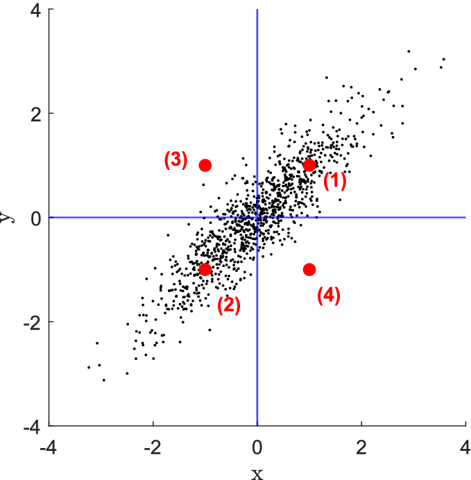

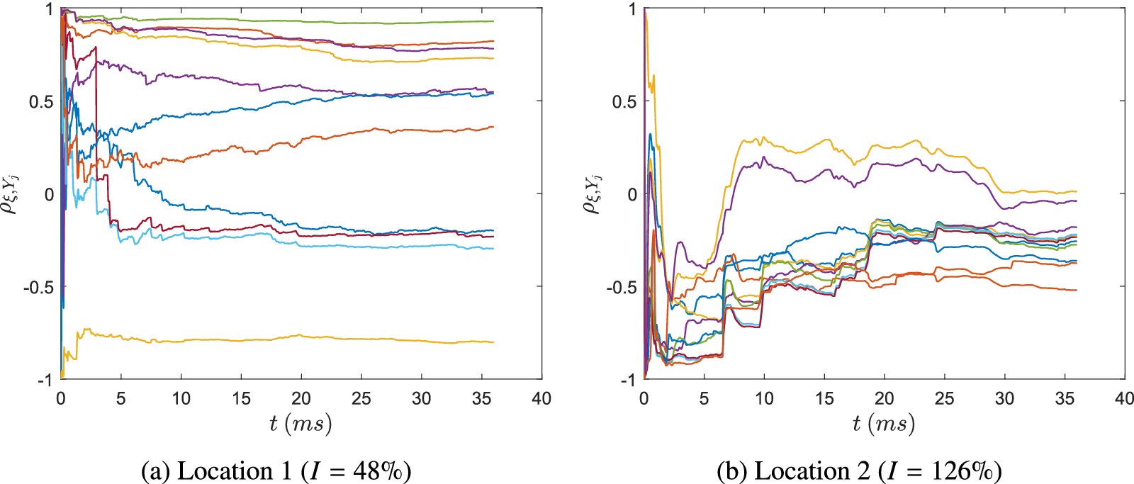

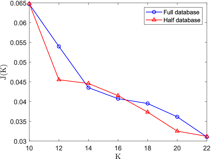


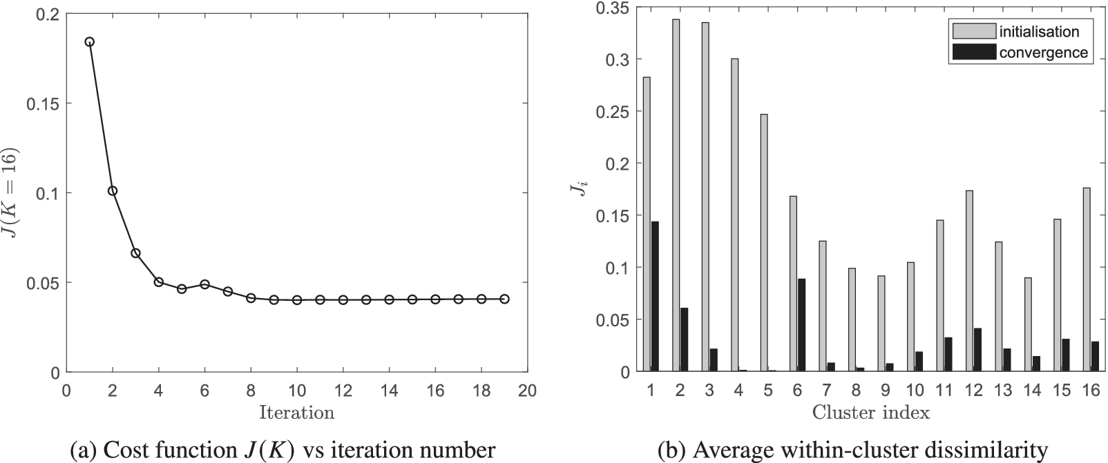


 Open access
Comments
No Comments have been published for this article.