Psychiatry is unique among medical disciplines in that often psychiatrists place almost total reliance on clinical acumen when making a diagnosis, rather than having the back-up of ‘diagnostic’ tests on which physicians and surgeons increasingly rely. There are three corollaries to this. First, psychiatry is a more cerebral discipline, requiring greater consideration and thought than most. Second, psychiatrists are probably less accurate in making the correct diagnosis, because they cannot rely on confirmation using histology, chemical pathology, haematology, radiology and electrophysiology. Consequently, they may need to be more prepared to revise their diagnoses than most clinicians. Third, the absence of a pathological/aetiological framework for diagnosis raises the challenging prospect that the diagnostic clusters used in psychiatry are wrong. Diagnosis in psychiatry currently has the same sophistication as did diagnosis by the 18th-century physician, who diagnosed on the basis of symptom clusters rather than aetiology or pathology. Someone presenting with fever and tremor in the 18th century would be diagnosed with ‘the ague’. Similarly, a patient with ankle swelling and ascites would be diagnosed as having ‘the dropsy’ (Reference Lyons and PetrucelliLyons & Petrucelli, 1987). Woe betide current medical students who consider these phenomena to be diagnoses, rather than signs of disease, and cannot recite numerous causes of pyrexia of unknown origin or oedema with ascites.
The CAGE questionnaire is commonly used as a brief screening test for alcohol dependence (Reference EwingEwing, 1984). It is scored on a five-point scale of 0–4. Ask most medical students (and some professors) what a positive test (such as a score of 2 out of 4) means and they are likely to answer that alcohol dependence is present. And if the test is negative (a score of 0, indicating no affirmative answers), then the condition is absent. This reductionist way of interpreting test results, although commonplace in medicine, is wrong: it is quite possible that someone scoring 4/4 on CAGE will not have alcohol dependence and someone scoring 0/4 will. Thankfully, in psychiatry this elemental approach to diagnostic tests is rare, but possibly only because psychiatrists use fewer tests than their colleagues in physical medicine.
The use of tests in psychiatry has always been widespread in research, as they are the main method of measuring outcome in clinical trials. Tests are also increasingly common in clinical practice; for example, neuropsychological testing in the diagnosis of dementia (Reference De Jager, Hogervorst and CombrinckDe Jager et al, 2003) or screening for depression in general practice (Reference Henkel, Mergl and KohnenHenkel et al, 2003). Therefore, whether for the purpose of interpreting results of clinical trials or for routine clinical practice, an understanding of the use of tests, their interpretation and limitations is helpful.
‘Tests’ tend to fall into two broad categories: those used for screening and those used for diagnosis. However, many of the principles used in understanding these different applications are similar.
Screening and diagnosis
There is an important difference between screening and diagnosis. Screening tests are designed to identify the possibility that disease might be present and to prompt further evaluation in those who screen positive. A screening test should therefore be regarded as only one possible first stage of the diagnostic sequence. For example, someone who scores 3 on the CAGE (i.e., screens positive) may then have a more in-depth interview about their drinking to identify the presence of a dependence syndrome (Reference Edwards and GrossEdwards & Gross, 1976). They may also have ‘confirmatory’ tests such as mean corpuscular volume, gamma-glutamyl transpeptidase or, ultimately, hepatic ultrasound and biopsy.
Screening tests should be easy to administer, acceptable to patients, have high sensitivity (i.e., identify most of the individuals with the disease), identify a treatable disorder and identify a disorder where intervention improves outcome (Reference Wilson and JungerWilson & Junger, 1968).
Diagnostic tests, on the other hand, are meant to provide the user with some surety that a disease is present.
No diagnostic test is 100% accurate, even those based on pathology results, although for the purposes of understanding the interpretation of tests it is necessary to suspend disbelief and assume that the reference standard (or gold standard) diagnostic procedure against which another test is compared is 100% accurate (Reference WarnerWarner, 2003). The reference standard test may be another questionnaire, a structured interview to provide diagnoses (e.g. using the DSM or ICD) or an interview with a clinician. Rarely in psychiatry, the reference standard may be derived from pathology, such as brain histopathology in dementia studies.
How helpful are tests in detecting disease?
Having established that a positive test does not always mean that the disorder tested for is present, it is possible to begin to explore how accurate a particular test is in correctly identifying disease when it is present and correctly excluding disease when it is absent.
Example 1: The usefulness of the CAGE
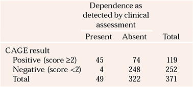
Reference Bernadt, Mumford and TaylorBernadt et al(1982) studied the usefulness of the CAGE in a psychiatric setting. Out of a sample of 371 patients on a psychiatric unit, 49 were diagnosed as having alcohol dependence, on the basis of a comprehensive assessment by clinicians, which was the reference standard in this study. The authors compared these assessments with the sample's CAGE results, using a score of 2 or more to indicate a positive result, i.e. alcohol dependence. The CAGE was positive for 45 of these 49 patients, i.e. it correctly identifying 92% of those thought to have alcohol dependence by the clinicians. (This is the CAGE's sensitivity.) However, using this 2/4 cut-off, the CAGE missed 4 patients (8%) defined by the reference standard as having alcohol dependence. Of the 322 patients thought not to have alcohol dependence by a clinician, 248 scored <2, i.e. below the cut-off. Thus, the CAGE correctly excluded 77% of those who did not have alcohol dependence. (This is its specificity.) The CAGE incorrectly suggested that 74 people had alcohol dependence when the reference standard of the clinical assessment said they did not.
These results are shown in Table 1. The format of this table, often referred to as a 2×2 table, is conventional for presenting such data. The results of the reference standard are given in the columns, and those of the diagnostic or screening test in the rows. The results of the reference standard are read vertically, down the columns of the table. To see how the other test (screening or diagnostic) performed, read horizontally, across the rows. Not all authors use this convention of putting the reference standard at the top of the table.
Table 1 Comparison of clinician-assessed (the reference standard) and CAGE-identified alcohol dependence (n = 371)
| Dependence as detected by clinical assessment | |||
|---|---|---|---|
| Present | Absent | Total | |
| CAGE result | |||
| Positive (score ≥2) | 45 | 74 | 119 |
| Negative (score <2) | 4 | 248 | 252 |
| Total | 49 | 322 | 371 |
Sensitivity and specificity
The sensitivity of a test is the proportion of individuals with a specific disease that the test correctly identifies as having it. So in Example 1, the CAGE, using a cut-off of >2 positive items as the threshold for caseness, has a sensitivity of 0.92 or 92%. The proportion that have the disease but are not identified as having it gives the test's false-negative rate. The CAGE missed 4 cases, so has a false-negative rate of 8%. The specificity is the proportion of individuals without the disease who are correctly identified by the test as not having it. In our example, the specificity of the CAGE is 0.77 or 77%. The false-positive rate is given by the proportion identified as having the disease that does not have it. The CAGE incorrectly suggested that 74 people had alcohol dependence, giving it a false-positive rate of 23%.
The ideal test is one that has very high sensitivity and specificity, so that most true cases are identified and most non-cases are excluded. However, sensitivity and specificity change in opposite directions as the cut-off (cut-point) of a test changes, and there is a trade-off between maximising sensitivity or specificity. For example, if the threshold for diagnosing alcohol dependence using the CAGE were to be made more demanding by increasing it to 3 or more positive answers (a score of ≥3), some patients who were truly alcohol dependent would no longer be identified by the test, so its sensitivity would decrease. On the other hand, using a ≥3 cut-off would mean that fewer patients would be mis-identified as possibly having alcohol dependence when they did not, so the specificity would increase. The sensitivity and specificity always have this inverse relationship.
Positive and negative predictive values
Sensitivity and specificity are characteristics of how accurate a test is. This is not particularly important to patients, who are much more likely to want to an answer to the questions ‘If I score positive for a test, what is the likelihood that I have the disease’, or ‘If I score negative, what is the likelihood I don't have the disease’. To answer these questions, refer again to Table 1, but this time look horizontally, across the rows. Reading along the row marked ‘Positive’, a total of 119 people scored positive on the CAGE, but only 45 (38%) had alcohol dependence as defined by the reference standard. This is the test's positive predictive value (PPV). For the 252 individuals who scored negative on the CAGE, 248 did not have alcohol dependence as defined by the reference standard: a negative predictive value (NPP) of 98%.
Unlike sensitivity and specificity, the PPV and NPV will change with the prevalence of a disease. For rare diseases, the PPV will always be low, even when a test is near perfect in terms of sensitivity and specificity.
Example 2: Near-perfect risk assesment of a rare event
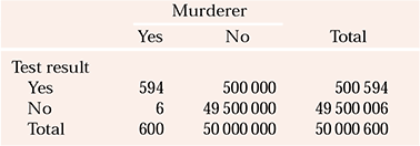
Table 2 compares data on murders committed in England with the results of an imaginary near-perfect (sensitivity and specificity of 99%) test designed to identify who will commit murder. The figures are invented but are close enough to make the point. Unfortunately, a real test of this accuracy is unavailable, and current predictive tests of human behaviour have much lower sensitivities and specificities (closer to water divining!), so the PPV will be much lower than in this example.
Table 2 Number of individuals who commit murder in one year compared with the number predicted by a fictitious, near-perfect test to identify murderers
| Murderer | |||
|---|---|---|---|
| Yes | No | Total | |
| Test result | |||
| Yes | 594 | 500000 | 500594 |
| No | 6 | 49500000 | 49500006 |
| Total | 600 | 50000000 | 50000600 |
About 600 murders are committed in England every year, which for the purposes of this example are attributed to 600 different murderers. So if our imaginary test, which predicts murderers with a sensitivity of 99%, was applied to all 50 million people in England, 594 murderers would be identified in advance and 6 will be missed. This sounds quite good, but consider the fact that all but 600 of the 50000000 people will not commit murder. With a specificity of 99%, 49500000 will be correctly excluded, but 500000 non-murderers will be incorrectly labelled as potential murderers. In this example, the PPV = 1.1%. Consequently, if this test existed and were used to prevent murder by incarcerating people deemed to present a risk, to prevent 594 murders 500594 people would need to be imprisoned. Remember, in the real world, the PPV will be considerably lower than in this example, because no test of such accuracy exists. If the sensitivity and specificity were 80% (still higher than can be currently achieved in this area) 10000000 non-murderers would need to be incarcerated to prevent 480 of the 600 murders. The fact that rare events inevitably have a low PPV is one reason why risk assessments have limited clinical utility.
Deciding the cut-off points on diagnostic tests
Most tests in psychiatry have more than one possible score, and deciding where to place the cut-off that divides respondents into ‘disease present’ or ‘disease absent’ is not arbitrary. The score that is chosen as the cut-off is determined by maximising sensitivity (identifying all true cases), while not compromising specificity (excluding all true non-cases). Plotting the sensitivity and specificity on a graph known as a receiver operating characteristic (ROC) plot can help to determine the usefulness of a test and the optimal cut-off. In ROC plots, the sensitivity (that is, the true-positive rate) is plotted against the false-positive rate (determined as 1 minus the specificity: 1 – specificity) for various cut-offs of the test. An ideal test will have one cut-off with a sensitivity of 1 (100% identification of true cases) and a specificity of 1 (100% exclusion of non-cases), i.e. the point at the top left of the graph. Therefore the closest score to this point is often used as the cut-off for a test. A test that adds nothing to diagnostic accuracy will plot along a diagonal line at 45° to the axes. In real life, tests have ROC curves between these two extremes, and the greater the area under the curve (AUC), the more closely the test approximates to the ideal.
Example 3: ROC curves
Figure 1 shows ROC curves for two tests of cognitive function. The Mini-Mental State Examination (MMSE) is a brief test of cognitive function used to screen for dementia (Reference Folstein, Folstein and McHughFolstein et al, 1975). The MMSE scores between 0 (very impaired cognition) and 30 (very good cognition). The cut-off for suspecting dementia is usually taken as 24. The 3MS is a modified version of the MMSE (Reference McDowell, Kristjansson and HillMcDowell et al, 1997). In Fig. 1, the sensitivity and 1 – specificity of the MMSE and the 3MS, measured against the reference standard, is plotted for each test score (e.g. in the MMSE 30 − 0). If, say a cut-off of 29/30 is selected for the MMSE, so that all those scoring below 29 were suspected of having dementia, the sensitivity would be very high, but the specificity would be low (giving high false-positive rates). This point would appear on the graph near the top right. If a cut-off of 5/30 is used, the sensitivity would be low (lots of people scoring 6 and above would be told they did not have dementia) but the specificity high (very few people scoring below 5 would not have dementia). This would be near the bottom left of the graph.
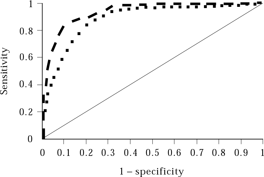
Fig. 1 A receiver operating characteristic curve comparing the MMSE (squares) with the 3MS (bars). The curves follow the plots of sensitivity and 1 – specificity (false positives) for each test score. The 3MS has a greater area under the curve (the space between the 45º diagonal line and the curve) and is closer to the ideal (sensitivity and specificity of 1); it is therefore possibly a better test (Source: Reference McDowell, Kristjansson and Hill McDowell et al, 1997 . © Elsevier Science, with permission.)
Exactly where the cut-off threshold is set depends on the purpose of the test: screening tests usually aim to be inclusive, with higher sensitivity, so that nearly all potential cases can be identified and assessed further. Diagnostic tests, especially those that lead to unpleasant treatments, tend to have greater specificity, so that false positives (identification of non-cases) are kept to the minimum.
Likelihood ratios
Sensitivity and specificity have limited use in day-to-day clinical practice and few clinicians will know this information when interpreting a test result. A more useful approach is to combine the sensitivity and specificity results into single measures that tell us how much more likely a positive or negative test result is to have come from someone with a disease than from someone without it. These are known as the likelihood ratios for a positive test (LR+) and for a negative test (LR−).
The LR+ is the likelihood of a positive test result when the diagnosis is present divided by the likelihood of a positive test result when the disease is absent. It can be calculated from the formula:
which provides a single number that can inform how useful a positive test is in clinical practice.
Similarly, the LR− can be calculated from:
Example 4: The LR+ and LR− for ≥2 on the CAGE
Using the sensitivity and specificity calculated in Example 1 from the values in Table 1, we can calculate the LR+ and LR− for scoring 2 or more on the CAGE:


You need calculate the likelihood ratios only once, as they will not change for different patients, provided the setting that the test was validated in is similar to that for the patients in question. The likelihood ratios do not change with different prevalences.
Pre- and post-test probabilities
Likelihood ratios are a useful way of informing you how much more (or less) likely a condition is, given a positive (or negative) test. To use likelihood ratios, it is important to have a sensible estimate of the probability that a condition is present before the test is done. This pre-test probability may be based on evidence (such as epidemiological studies of prevalence) and/or clinical intuition after assessing a patient.
Example 5: Estimating pre-test probablity
Try to answer these questions below, using only the information provided and your clinical experience:
-
• If I see a patient at 11.00 a.m. in out-patients with anxiety, what is the probability he or she has alcohol-dependence syndrome?
-
• If I see a middle-aged man at 11.00 a.m. in out-patients with anxiety and he smells of alcohol what is the probability he has alcohol-dependence syndrome?
-
• If I see a middle-aged man at 11.00 a.m. in out-patients with anxiety and he smells of alcohol, looks dishevelled and has a ruddy complexion, what is the probability he has alcohol-dependence syndrome?
Most people would have a different answer for each scenario, with the probability rising significantly for the last one. Our clinical estimation of pre-test probability is quite subtle and is likely to change with each additional piece of information.
Once some sensible estimate has been made, the use of a screening or diagnostic test with a known likelihood ratio can then provide a post-test probability.
Example 6: Estimating a post-test probability
We found in Example 4 that the LR+ in psychiatric patients scoring ≥2 on the CAGE is 4. ‘Odds’ is the number of events divided by the number of non-events. From Table 1, the odds of alcohol dependence in the overall sample (the pre-test odds) are 49/322 or 0.15. The odds of alcohol dependence being present in those positive for the test (the post-test odds) are 45/74 or 0.61. These odds and the LR are linked: Bayes’ theorem states that
In other words, in our example a positive likelihood ratio of 4 means that the odds of a disease being present in those positive for the test are 4 times greater than the odds of diagnosis in the original sample, before the test was applied. Unfortunately, we cannot multiply a probability by a likelihood ratio: probabilities need to be converted to odds before the likelihood ratio can be used.
Example 7: Using odds and probabilities to improve on clinical assessment
If statistics don't captivate you, feel free to skip this example.
Can a patient's CAGE score better your clinical assessment of the likelihood that he has alcohol dependence? The following relationships are given:
Assume that you see a man in out-patients and after an initial clinical assessment you think there is a 30% chance he has alcohol dependence. He then completes the CAGE with a cut-off of ≥2 and scores positive.
The pre-test probability for our CAGE example is 0.3. Convert this to odds using formula (a) above:
Thus, the pre-test odds of this patient having alcohol dependence are 0.43.
Then, using formula (c),
i.e. the post-test odds of this patient having alcohol dependence are 1.7.
Converting these odds back to a probability using formula (b)
Thus, the post test-probability is 0.63. So, by applying the CAGE and finding that the patient scores 2 or more, the likelihood that he has alcohol dependence has risen from 30% (the clinician's initial assessment) to 63%.
The likelihood-ratio nomogram
Fortunately, you do not have to do the maths of converting probabilities to odds and back again to use likelihood ratios. The Fagan likelihoodratio nomogram (Fig. 2) provides a simple non-mathematical method of determining post-test probabilities. The nomogram is widely available in books on critical appraisal. To use the likelihood-ratio nomogram:
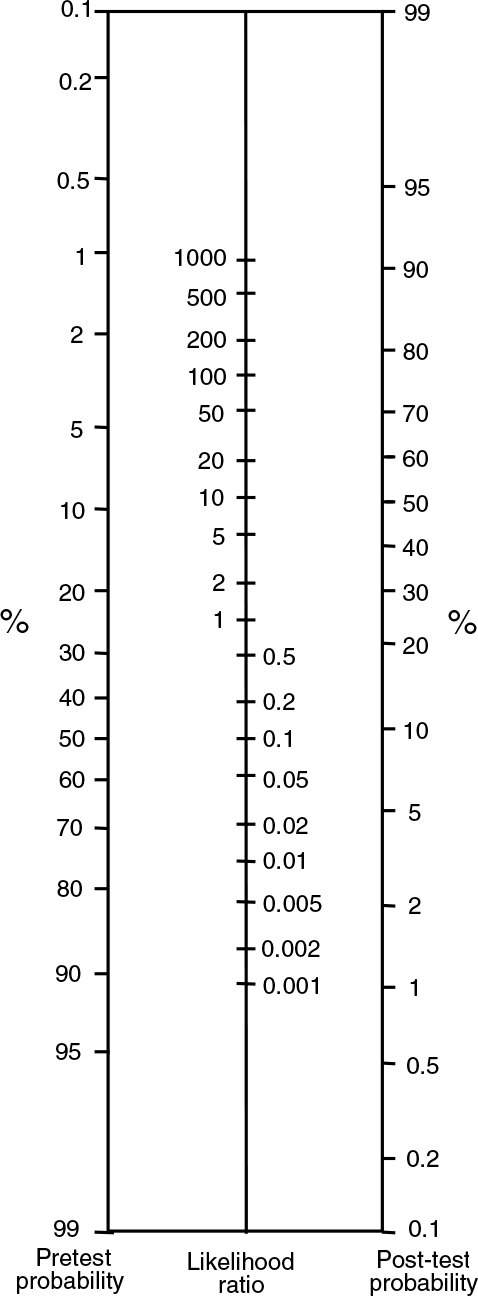
Fig. 2 Fagan likelihood-ratio nomogram. (Source: Reference FaganFagan, 1975. © 1975 Massachusetts Medical Society, with permission.)
-
1 Estimate the pre-test probability, (i.e. the likelihood of a disease being present before you know the test result).
-
2 Calculate the LR+ and/or LR−.
-
3 Using a straight edge, draw a line through the pre-test probability and the LR.
-
4 Read off the post-test probability from the right-hand column.
Example 8: Using the likelihood-ratio nomogram
Following steps 1 to 4 and using the data from our CAGE example above for a patient with a positive result (a pre-test probability of 30% and an LR+ of 4) and drawing a line through 30% and 4, we read from from the right-hand column that the post-test probability is just over 60% (in Example 7 we used maths to show that the result is 63%). Thus, you are now more sure that the patient has alcohol dependence.
The LR− for CAGE is 0.1. So, for someone who scores less than 2 on the CAGE (a negative test) with a pre-test probability of 30%, the post-test probability falls to about 4%, almost ruling out alcohol dependence.
Note what happens if you change the pre-test probability. If the pre-test probability is 1%, given a positive CAGE result, the post-test probability is still less than 5%. This is unlikely to make any difference to diagnosis or management. This is a general property of diagnostic tests – if the pre-test probability is very low, diagnostic tests are of little practical value (cf. Table 2).
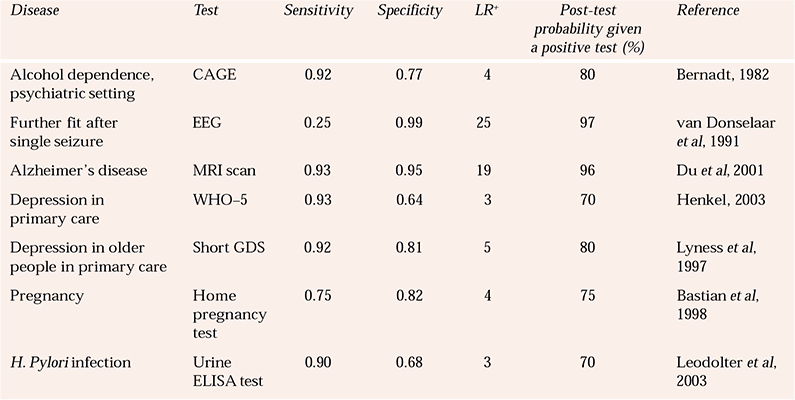
More examples of tests and their likelihood ratios are given in Table 3. For all of the examples in that table, I have assumed a pre-test probability of 50%. You could experiment with different pre-test probabilities using the nomogram. It is interesting to see that the results for home pregnancy-testing kits and laboratory tests for H. pylori infection are also provided to show some ‘chemical’ tests fare little better than the tests used in psychiatry!
Table 3 Sensitivities, specificities and likelihood ratios for some tests used in psychiatry and general health. The post-test probabilities are based on a pre-test probability of 50% for each condition
| Disease | Test | Sensitivity | Specificity | LR + | Post-test probability given a positive test (%) | Reference |
|---|---|---|---|---|---|---|
| Alcohol dependence, psychiatric setting | CAGE | 0.92 | 0.77 | 4 | 80 | Reference Bernadt, Mumford and TaylorBernadt, 1982 |
| Further fit after single seizure | EEG | 0.25 | 0.99 | 25 | 97 | Reference van Donselaar, Geerts and Schimsheimervan Donselaar et al, 1991 |
| Alzheimer's disease | MRI scan | 0.93 | 0.95 | 19 | 96 | Reference Du, Schuff and AmendDu et al, 2001 |
| Depression in primary care | WHO–5 | 0.93 | 0.64 | 3 | 70 | Reference Henkel, Mergl and KohnenHenkel, 2003 |
| Depression in older people in primary care | Short GDS | 0.92 | 0.81 | 5 | 80 | Reference Lyness, Noel and CoxLyness et al, 1997 |
| Pregnancy | Home pregnancy test | 0.75 | 0.82 | 4 | 75 | Reference Bastian, Nanda and HasselbladBastian et al, 1998 |
| H. Pylori infection | Urine ELISA test | 0.90 | 0.68 | 3 | 70 | Reference Leodolter, Vaira and BazzoliLeodolter et al, 2003 |
Appraising articles about diagnosis
As with other sources of evidence, such as randomised trials of therapy or studies on prognosis or aetiology, articles on diagnostic tests should be critically appraised before the evidence is used to inform clinical practice (Reference Jaeschke, Guyatt and SackettJaeschke et al, 1994a ,Reference Jaeschke, Guyatt and Sackett b ). Critical appraisal of an article on diagnostic tests has three components. These are:
-
• deciding to what extent the study is valid
-
• assessing how useful the results are
-
• assessing whether the study is applicable to you and your patients.
Validity
When deciding whether to use a diagnostic or screening test, it is important to consider the internal validity of the study evaluating the test (Box 1).
Box 1 Critical appraisal: are the results valid?
Was the reference standard appropriate for the study?
The reference standard with which a test is compared has to have face validity and be relatively accurate. Remember that no test (including those used as reference standards) is 100% accurate.
Was there an independent blind comparison with the reference standard?
The central issue in studies on diagnostic/screening tests is the comparison of the test under scrutiny with the reference standard. The aim is to identify how the test performs in terms of both identifying the disease/condition when the reference standard identifies it as present (sensitivity), and excluding it when the reference standard says it is absent (specificity). For this comparison to be accurate, the person performing/interpreting the test must be blind to the results of the reference standard and vice versa.
Was the test evaluated in a sufficient number of people at risk of the disease?
If the study sample was relatively small, the sensitivities and specificities will have low precision and any conclusions on the usefulness of the test may be misleading.
Did the sample include a spectrum of patients appropriate to your purposes?
The sensitivity and specificity of a test will change according to the population being tested. Therefore there may be little point relying on these measures if the trial involved a population from a specialist tertiary referral centre but you want to know how the test performs in a primary care setting.
Did the results of the test influence the decision to perform the reference standard?
This may seem a strange question at first, but some evaluations of screening tests apply the reference standard only to those testing positive for the screening test. This is particularly common where the reference standard is lengthy. If this is done, you cannot know what the true false-negative rate is (see Box 2). It may be acceptable to apply the reference standard to a random selection of those screening negative, but the ideal is to give everyone in the study both tests.
Was the method for performing the test described in sufficient detail?
Subtle changes in the way a test is performed can make significant changes to the results. Look for a clear description of the method of both the reference standard and the test under scrutiny.
Usefulness
The usefulness of the results (Box 2) of a test are best thought of in terms of likelihood ratios, which you may have to calculate yourself, as they are rarely given in articles.
Box 2 Critical appraisal: are the results useful?
Are the likelihood ratios for the test presented (or can you calculate them)?
Usually, you can create a 2×2 table (such as Table 1) from the data given. The data may be presented ‘raw’ or you may need to back-calculate them. If the sensitivities and specificities are reported, you will need to re-form the 2×2 table only if you want to know the positive or negative predictive values (respectively, PPV and NPV, very useful measures). Make sure that you get the table axes the right way round. The table should look like this:

| Reference standard | |||
|---|---|---|---|
| Disease present | Disease absent | ||
| Test positive | a (true +ve) | b (false +ve) | a+b |
| Test negative | c (false −ve) | d (true −ve) | c+d |
Useful related formulae:
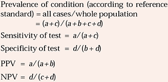
The likelihood ratio (LR) is a useful way of combining sensitivity and specificity. Most articles do not report the LR, but they can be calculated as in Example 4.
You can use the LR to identify the post-test probability using the nomogram shown in Fig. 2 or the four-step procedure followed in Example 8.
How precise are the sensitivity and specificity?
Sensitivities and specificities should be presented with confidence intervals, to provide a measure of precision of the estimates.
Applicability
The applicability of a test in clinical practice depends on several issues. First, the study assessing the test should be based on a sample with socio-demographic and clinical characteristics similar to the people on whom you want to use it. Although likelihood ratios do not change with prevalence, they may change significantly when the test is applied in different populations. An interesting example here is the CAGE questionnaire again; the likelihood ratio was much higher when the CAGE was validated in a primary care setting (LR+ = 12) (Reference Liskow, Campbell and NickelLiskow et al, 1995) than in a psychiatric setting (LR+ = 4) (Reference Bernadt, Mumford and TaylorBernadt et al, 1982). This may be because many individuals with mental disorder are more likely to report guilt or get annoyed, even when they do not drink much. Other applicability issues include whether the test is readily available and acceptable to the patient, and whether the results are easy to interpret and lead to a change in management of the patient (Box 3).
Box 3 Critical appraisal: will the results help me in caring for my patient?
Is the test available and easily performed?
Look specifically at how you can perform the test in your setting. Do you require any special equipment?
Is there a sensible estimate of pre-test probability?
Pre-test probability is the probability a patient has an illness determined before the test is performed. You may use clinical intuition for a particular patient, or base the pre-test probability on existing prevalence data.
Will the results change how I manage this patient?
This is worth considering. Is it ever necessary to perform a test: (a) if it has such a low likelihood ratio that it has little or no effect on your decision of whether a condition is present; or (b) if the prevalence of a condition is very low?
Will the patient be better off if the test is performed?
Even if the test is valid and reliable, with a high likelihood ratio, if the patient will not benefit from the disease being identified there may be little point in performing it.
Other issues
Other issues that may influence your use or interpretation of a test include interrater reliability, which is a measure of how closely different raters agree when using a particular instrument to assess particular patients. This may be especially important if different members of your team use the same assessment tool. Interrater reliability for categorical variables (such as disease present/disease absent) is measured using kappa, which assesses the degree of concordance after taking into account that some agreement between raters will occur by chance. A kappa value >0.6 is generally held to indicate good interrater agreement (Reference Guyatt and RennieGuyatt & Rennie, 2002). Not all instruments, especially those used in research, have good interrater reliability. For example, the Clinicians’ Interview-Based Impression of Change (CIBIC), a seven-point scale which is widely used as an outcome measure for dementia studies, has an interrater kappa value of 0.18, indicating very poor reliability (Reference Quinn, Moore and BensonQuinn et al, 2002).
Conclusions
‘We are inclined to believe those whom we do not know because they have never deceived us.’
(Samuel Johnson, 1709–1784)
Samuel Johnson's words sum up the usefulness of understanding critical appraisal of diagnostic tests, by emphasising that nothing should be taken at face value without further exploration and assessment. This applies in particular to areas of psychiatry that have remained relatively undisturbed by the evidence-based medicine bandwagon, for example the utility of diagnostic tests. Without appraisal skills in this area, be prepared to be deceived!
MCQs
-
1 The following should be considered when assessing the internal validity of a study evaluating a new screening instrument:
-
a whether earlier recognition of the condition is beneficial to the patient
-
b whether both the screening and the reference standard were applied blind
-
c the cost of using the instrument
-
d whether the patients on whom the instrument was assessed are similar to yours
-
e the positive predictive value of the instrument.
-
-
2 The following indicate that a diagnostic test may be unsuitable for your patients:
-
a the positive predictive value is 80%
-
b the likelihood ratio for a positive test is 2
-
c the prevalence of the disorder in your patients is 1%
-
d interrater reliability (kappa) of the test is 0.8
-
e your patients are much older than those in the study used to validate the test.
-
-
3 A new test for anxiety has a sensitivity of 80% and specificity of 90% against the reference standard ICD–10 diagnosis. Which of the following statements is true:
-
a all individuals scoring positive on this test will have anxiety disorder
-
b the false-positive rate is 10%
-
c if the pre-test probability is 10%, the positive predictive value is 70%
-
d the likelihood ratio for a positive test is 8
-
e the test should definitely be used in routine practice.
-
-
4 The following statements are true:
-
a kappa is a measure of interrater reliability that takes into account chance agreement
-
b the optimal cut-off of a screening test is decided using a funnel plot
-
c screening tests ideally have high specificity
-
d the diagnostic tests in psychiatry are usually less discriminating than those used in physical medicine
-
e the likelihood-ratio nomogram is used to determine post-test probability.
-
-
5 In a clinical assessment you estimate that the chance that the patient is depressed is 10%. She subsequently scores positive on a depression screening instrument for which LR + = 10. Taking into account the postive test result, the likelihood-ratio nonogram shows that the probability that she has depression is roughly:
-
a 15%
-
b 30%
-
c 55%
-
d 85%
-
e 100%.
-
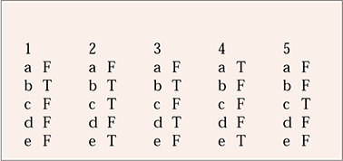
MCQ answers
| 1 | 2 | 3 | 4 | 5 | |||||
|---|---|---|---|---|---|---|---|---|---|
| a | F | a | F | a | F | a | T | a | F |
| b | T | b | T | b | T | b | F | b | F |
| c | F | c | T | c | F | c | F | c | T |
| d | F | d | F | d | T | d | F | d | F |
| e | F | e | T | e | F | e | T | e | F |



eLetters
No eLetters have been published for this article.