Introduction
Insect-resistant crops that have a gene from the soil bacterium Bacillus thuringensis (Bt) are now one of the most widely adopted genetically-modified (GM) crop varieties in the world. In particular, single-trait Bt corn and cotton varieties have been used in developed and developing countries, primarily to control lepidopteran pests that can damage these crops (e.g., Asian/European corn borer, cotton bollworm). Given the widespread use of these single-trait Bt crops, there have been studies investigating the yield and insecticide use effects of this Bt technology in both developed and developing countries (See Smale, Zambrano, and Cartel Reference Smale, Zambrano and Cartel2007 and Qaim Reference Qaim2009 for a comprehensive review of this literature).
In general, these studies found that first-generation Bt crops have yield-increasing and pesticide-reducing effects. For example, yield-increasing effects of Bt cotton are largest for countries that typically underuse pesticides, such as in Argentina (Qaim and De Janvry Reference Qaim and De Janvry2005), India (Qaim Reference Qaim2003), and South Africa (Shankar and Thirtle Reference Shankar and Thirtle2005). While in countries where pesticide use is typically high, such as China and the United States, the pesticide-reducing effect of Bt cotton is much more dominant than the yield-increasing effect (Falck-Zepeda et al. Reference Falck-Zepeda, Traxler and Nelson2000, Huang et al. Reference Huang, Hu, Rozelle, Qiao and Pray2002). Although there are only few studies examining the effects of Bt corn, the existing literature also shows similar yield-increasing and insecticide-reducing effects, albeit with a smaller magnitude (Brookes and Barfoot Reference Brookes and Barfoot2005, Fernandez-Cornejo and Li Reference Fernandez-Cornejo and Li2005, Gouse et al. Reference Gouse, Pray, Schimmelpfennig and Kirsten2006, Yorobe and Quicoy Reference Yorobe and Quicoy2006, Qaim Reference Qaim2009, Nolan and Santos Reference Nolan and Santos2012, Shi, Chavas, and Lauer Reference Shi, Chavas and Lauer2013).
Aside from the yield and insecticide use effects of Bt crops, recent studies examine the production risk effects of using Bt technology.Footnote 1 Crost and Shankar (Reference Crost and Shankar2008), using panel data and a stochastic production function approach, observed a risk-reducing effect for Bt cotton in India, but they found no conclusive evidence for the risk effects of Bt cotton in South Africa. Using a stochastic production function approach with a single year of cross-sectional data, Shankar et al. (Reference Shankar, Bennett and Moorse2007, Reference Shankar, Bennett and Morse2008) also investigated the production risk effects of Bt cotton in South Africa and found that Bt cotton significantly increases yield (or output) risk.
Hurley et al. (Reference Hurley, Mitchell and Rice2004) developed a theoretical model showing Bt corn as risk increasing or risk decreasingFootnote 2 and then used a simulation model for two counties in the United States to empirically verify their theoretical results. Using experimental field trial data from 1990 to 2010, Shi, Chavas, and Lauer (Reference Shi, Chavas and Lauer2013) found that transgenic corn (i.e., single-trait Bt for corn borer and other multi-trait GM corn) lowers production risk as measured by variance, skewness and kurtosis of harvested yields. Krishna, Qaim, and Zilberman (Reference Krishna, Qaim and Zilberman2016), using the same production risk measures used by Shi, Chavas, and Lauer (Reference Shi, Chavas and Lauer2013), found that Bt cotton increases mean yield and reduces production risks, based on panel data from a farm survey in India. The risk studies mentioned above are consistent with earlier empirical literature that shows that it is possible for pest control inputs to either be risk-increasing (Horowitz and Lichtenberg Reference Horowitz and Lichtenberg1993) or risk-decreasing (Smith and Goodwin Reference Smith and Goodwin1996).
While these studies have investigated the production risk effects of Bt technology, no study (to our knowledge) has looked at how Bt technology affects yield skewness. With the exception of Shi, Chavas, and Lauer (Reference Shi, Chavas and Lauer2013) and Krishna, Qaim, and Zilberman (Reference Krishna, Qaim and Zilberman2016), the papers that have studied production risk effects of Bt only typically considered mean yield and yield variance impact of Bt technology (i.e., a mean-variance approach). An increase in the skewness of yields means a reduction in downside risk (i.e., a decrease in the probability of crop failure).Footnote 3 The effect of an input on the skewness of output provides additional information that is not apparent when only looking at the effect of input on the variance of output. Farmers with decreasing absolute risk aversion (DARA) preferencesFootnote 4 would be more averse to exposure to downside risk (Menezes et al. Reference Menezes, Geiss and Tressler1980, Antle Reference Antle1987) and would have more incentives to adopt the Bt crop if there is evidence that it does significantly increase yield skewness.
Moreover, most of the studies that used a moment-based approach to capture the mean, variance, and skewness effects (e.g., Di Falco Reference Di Falco2006, Di Falco and Chavas Reference Di Falco and Chavas2009, Krishna, Qaim, and Zilberman Reference Krishna, Qaim and Zilberman2016) do not recognize the damage-abating nature of insecticides and Bt technology. Lichtenberg and Zilberman (Reference Lichtenberg and Zilberman1986) argue that damage-abating inputs such as pesticides are different from conventional inputs (e.g., fertilizer and labor) in that they affect output only indirectly by reducing the extent of any damage that may occur. In contrast, conventional inputs affect output directly. Given that the marginal productivity of pesticide use is intimately related to Bt corn adoption in farmers’ fields, accounting for the damage control nature of this technology in the functional form is important in our empirical context (Mutuc et al. Reference Mutuc, Rejesus and Yorobe2011, Nolan and Santos Reference Nolan and Santos2012).
The objective of this paper is to determine the production risk effects of Bt corn in the Philippines. Specifically, we examine the impact of single-trait Bt corn on the mean, variance, and skewness of yields, and then evaluate the welfare implications of these effects using risk premium and certainty equivalent measures. The analysis relies on farm-level survey data collected in the Philippines in the 2007/2008 crop years. We build on the stochastic production function approach of Saha et al. (Reference Saha, Shumway and Havenner1997) to account for the damage-abating nature of Bt (and other pesticides) when analyzing its risk effects. We extend this model to examine the downside risk effects (i.e., skewness effect) of Bt corn within a damage-abatement specification. This extension is a methodological contribution to the literature because, to the best of our knowledge, this is a new approach to analyze the downside risk effects of damage-abating technologies in general (not just Bt).
Our empirical results indicate that the main benefit of Bt corn in the Philippines is through its mean yield-increasing effect and downside risk-reducing effect (i.e., skewness-increasing). The results also indicate that Bt corn in the Philippines has a statistically significant risk-increasing effect (i.e., variance-increasing). However, this does not lead to higher risk premiums because the mean yield and skewness effects outweigh the variance effect. Our certainty equivalent measure indicates that Bt corn farmers in the Philippines tend to be better off than non-Bt farmers, given Bt corn's dominant yield-increasing and downside risk-reducing effects.
Conceptual Framework
A stochastic production function can be expressed as: y = g(Bt, x, v), where y is the quantity of corn produced, Bt represents a dummy variable, 1 = Bt corn adopter, 0 = non-adopter, x is a vector of all the other inputs, and v is a vector of unobserved factors not under the control of the producer (i.e., unobserved weather variables, production or pest conditions). The profit of the producer is π = p·g(Bt, x, v) − c(Bt, x), where p > 0 is the output price and c(Bt, x) is the cost of input Bt and all the other inputs. Assume that the utility of the farmer depends on profit (e.g., U(π)) and is characterized by a von Neumann-Morgenstern utility function. Expected utility of the farmer can then be defined as (Pratt Reference Pratt1964):
where R is the risk premium that measures the cost of private risk bearing. The certainty equivalent (CE), the sure amount of profit the farmer would be willing to receive that would give the same utility as the expected value of the random profit, is:
From (1) and (2), the risk premium (R) and the certainty equivalent (CE) depend on the moments of profit, which in turn hinge on the moments of the production function g(Bt, x, v). By taking a Taylor series approximation on (1) evaluated at the point E(π), one can derive the following expression (See Di Falco Reference Di Falco2006, Di Falco and Chavas Reference Di Falco and Chavas2009):Footnote 5
From (3), the risk premium R a can then be approximated as follows:
where M i = E[π − E(π)] i is the ith central moment of the profit distribution, r 2 = −(∂2 U/∂π2)/(∂U/∂π) is the Arrow-Pratt coefficient of absolute risk aversion, and r 3 = −(∂3 U/∂π3)/(∂U/∂π), all evaluated at E(π). Equations 3 and 4 allow us to decompose the effect of variance and skewness on the risk premium of the producer. Under risk aversion behavior (i.e., when (∂2 U/∂π2) < 0 and r 2 > 0), an increase in profit variance would result in higher risk premium (or higher cost of private risk bearing). For the effect of the skewness of the profit distribution on the risk premium, Di Falco (Reference Di Falco2006), Di Falco and Chavas (Reference Di Falco and Chavas2009) show the risk premium tends to decrease with a rise in skewness, assuming that farmers have downside risk aversion (i.e., when (∂3 U/∂π3) > 0 and r 3 < 0). We can empirically estimate the effect of Bt corn on risk premiums (and CE) from (4) by assuming that p is known (i.e., risk only depends on the moments of the production distribution).
To account for the damage abating nature of pesticides and Bt corn, we apply the Di Falco (Reference Di Falco2006), Di Falco and Chavas (Reference Di Falco and Chavas2009) moment-based approach to study the downside risk exposure in the model in Saha et al. (Reference Saha, Shumway and Havenner1997). The model has a flexible risk representation that allows one to ascertain the effects of conventional and damage abating inputs on output variance and skewness. The damage abatement production function as presented in Saha et al. (Reference Saha, Shumway and Havenner1997) is:
where x is a vector of conventional or direct production inputs, z is a vector of damage abating inputs such as pesticide and Bt corn, β and α are parameters to be estimated, and e and ε are error terms. Note that e, which is associated with the damage abatement function h(·), represents pest- and pesticide-related randomness ordered from good states to bad states (i.e., lower to higher unobserved pest density) and ε represents randomness related to crop growth conditions ordered from bad states to good states (e.g., poor rainfall to good rainfall). Following Saha et al. (Reference Saha, Shumway and Havenner1997), we make two assumptions on (5) to facilitate identification and estimation: (i) the damage abatement function is specified as h(z, α, e) = exp[−A(z, α) e] where A(·) is a continuous and differentiable function, and (ii) the two error terms have the following properties, ε ~ N(0,1), e ~ (μ,1), and cov(ε,e) = ρ. Under these assumptions, the natural logarithm of output has a normal distribution:
where B(·) ≡ [ 1 + A(·)2 − 2 A(·)ρ] and is defined as the variance of ln(y). The implication of (6) is that output y is log-normally distributed (Saha et al. Reference Saha, Shumway and Havenner1997).Footnote 6 The probability density function (pdf) of this distribution is
And the moment of this distribution is
From (8), it is readily verified that the mean of the distribution is
For the second central moment (the variance),
and based on (8) the following equations hold
For the third central moment,
and based on (8):
Hence, after substituting ln f(·) − μA(·) in (6) for μ and B(·) for σ2 in (9)–(11), the mean, variance and the third central moment of output become
respectively. The specification above allows the damage abating inputs and technologies in h(·) to have marginal effects on the variance and skewness of output that are independent of the marginal effects on the expected value of input. The flexibility with respect to risk is retained while maintaining the damage abatement specification.
For damage control inputs, they only appear in function A(·) of the damage abatement function, not in the function f(·). Hence, the effects of damage control input, z k , where k = 1, 2, and 3 moment of the distribution, can be computed directly by differentiation of (12a)–(12c) with respect to z k , after some simplification:
 $$\eqalign{ \displaystyle{{\partial S\lpar y\rpar } \over {\partial z_k}} = \, &3\bar y^3 \lpar e^{B\lpar{\cdot}\rpar } - 1\rpar \lsqb \lpar \lpar e^{B\lpar{\cdot}\rpar } \rpar ^2 + e^{B\lpar{\cdot}\rpar } \rpar \lpar 3A\lpar{\cdot}\rpar - 3{\rm \rho} - {\rm \mu} \rpar - \lpar 2\lpar A\lpar{\cdot}\rpar \cr &- {\rm \rho} - {\rm \mu} \rpar \rsqb \cdot \displaystyle{{\partial A\lpar{\cdot}\rpar } \over {\partial z_k}}\comma \;}$$
respectively. We expect the Bt corn adoption coefficient has a positive sign in the production model to indicate that Bt technology increases yield, while a negative sign in the variance model to indicate that Bt technology reduces production risk. A positive sign in the skewness model would imply a reduction in downside risk exposure (Di Falco and Chavas Reference Di Falco and Chavas2009).
Bt Corn Status in the Philippines
Bt corn in the Philippines was mainly developed to be resistant to the Asian corn borer (Ostrinia furnacalis Guenee) (see Morallo-Rejesus and Punzalan Reference Morallo-Rejesus and Punzalan2002). The Asian corn borer is one of the most destructive corn pests in the country and typically accounts for 20–30 percent of annual crop damage (Dela Rosa Reference Dela Rosa2001). It damages plants by boring holes in the stems and pods that cause wilting of the leaves and crop losses. Bt corn carries a transplanted gene that produces a delta-endotoxin protein that paralyzes the larvae of some harmful insects, including Asian corn borers, when ingested. The Bt protein punctures the mid-gut of the insect, leaving it unable to eat, and it will eventually die within a few days.
Bt corn was commercially grown in the Philippines in 2003, seven years after it was first introduced on a limited trial basis. Monsanto, Pioneer Hi-Bred, and Syngenta are the three companies that sell Bt corn seeds in the country. Since 2003, farms planted to conventional hybrid corn varieties have been steadily replaced with Bt corn. From about 0.5 percent of the total area harvested to corn (i.e., 11,000 hectares) in 2003, James (Reference James2014) reports that Bt corn was planted on about 32.4 percent of the total area harvested (i.e., 831,000 hectares) in 2014. The Philippine Department of Agriculture (DA) stresses that the use of Bt corn is a means to ensure the country's food security and global competitiveness. The Philippine DA believes that Bt corn reduces farmers’ input costs and increases their yield, while keeping the ecosystem intact and enabling crops to grow under unfavorable conditions.
Data Description
The data used in this study are based on the International Food Policy Research Institute (IFPRI) corn surveys in the Philippines for crop years 2007/2008.Footnote 7 The cross-sectional data collected in the survey included information on corn farming systems and environment, inputs and outputs, costs and revenues, the marketing environment, and other factors related to Bt corn cultivation (i.e., subjective perceptions about the technology). Data were collected through face-to-face interviews using pre-tested questionnaires. The IFPRI survey only collected data from the largest parcel cultivated for each farmer respondent. Bt corn farmers are those farmers whose largest parcel was planted with Bt corn alone. Non-Bt farmers, on the other hand, are strictly farmers who plant hybrid corn in their largest parcel and other parcels (i.e., farmers that plant traditional open pollinated varieties are not included in the non-Bt sample). Restricting the non-Bt farmers to hybrid corn users allows one to more meaningfully see the performance difference between Bt corn relative to a more homogenous population of non-Bt farmers (i.e., hybrid corn users only).Footnote 8
To arrive at the study sample, two major corn-producing provinces (Isabela and South Cotabato) were initially selected due to the reportedly high use of both Bt and hybrid varieties in these provinces. Seventeen top corn-producing villages from four agricultural towns were then selected from the two provinces (i.e., four villages from the town of Tampakan in South Cotabato province, four villages from General Santos city in South Cotabato, four villages from the town of Cauayan in Isabela, and five villages from the town of Ilagan in Isabela). The list of yellow corn growers in the village was provided by the village head. Only smallholder corn farmers were included in the list. Smallholders were defined as those planting only 1–3 hectares in Isabela Province and 1–5 hectares in South Cotabato Province. These farm-size ranges were based on mean corn area per farm in these villages. In the third stage, 468 corn farmers were selected randomly from the list of smallholders in the 17 villages. After removing two observations with incomplete information and missing data, 466 observations (out of 468) are used in the analysis of the data from the 2007/2008 crop year (254 Bt adopters and 212 non-Bt adopters).
Estimation Procedures and Empirical Specification
In our analysis, the input variables, x, included in the stochastic production functions are seed (kg/ha), N fertilizer (kg/ha), insecticide (li/ha), and labor (manday/ha), as well as a Bt dummy variable. The dependent variable y is corn yield (ton/ha).
For our extension of the Saha et al. (Reference Saha, Shumway and Havenner1997) model, as expressed in (5), (6), and (12), the parameters (β, α, μ, ρ) are estimated directly using maximum likelihood estimation. From (6), the log-likelihood function of (5) can be represented as follows:
where i indexes the observations in this case. Akaike Information Criteria (AIC) and Bayesian Information Criteria (BIC) were the specification tests undertaken to determine which functional forms would best fit f(·) and A(·). The Cobb-Douglas functional form was found to be the best fit f(·), and A(·) and was used in our estimation procedures (linear, linear-log, and quadratic specifications are the other functional forms examined).
One issue that needs to be dealt with at this point is the possibility of selection problems due to the nonrandom selection of Bt adopters. There may be other observable farm-level variables (i.e., farming experience, education, etc.) that can affect yield (or risks) aside from Bt technology. It is also possible that there are unobservable variables (not included in the production function specification) that affect both the outcome variable y and the decision to adopt Bt. For example, it is likely that farmers who adopt Bt are those with better management ability (or are more efficient) than the non-Bt adopters. Because management ability is unobserved and not included in the stochastic production function specification, it can be that the observed difference between the yields (or risks) of Bt and non-Bt adopters is due to the systematic difference in management abilities between the two groups (i.e., not due to the Bt technology per se).
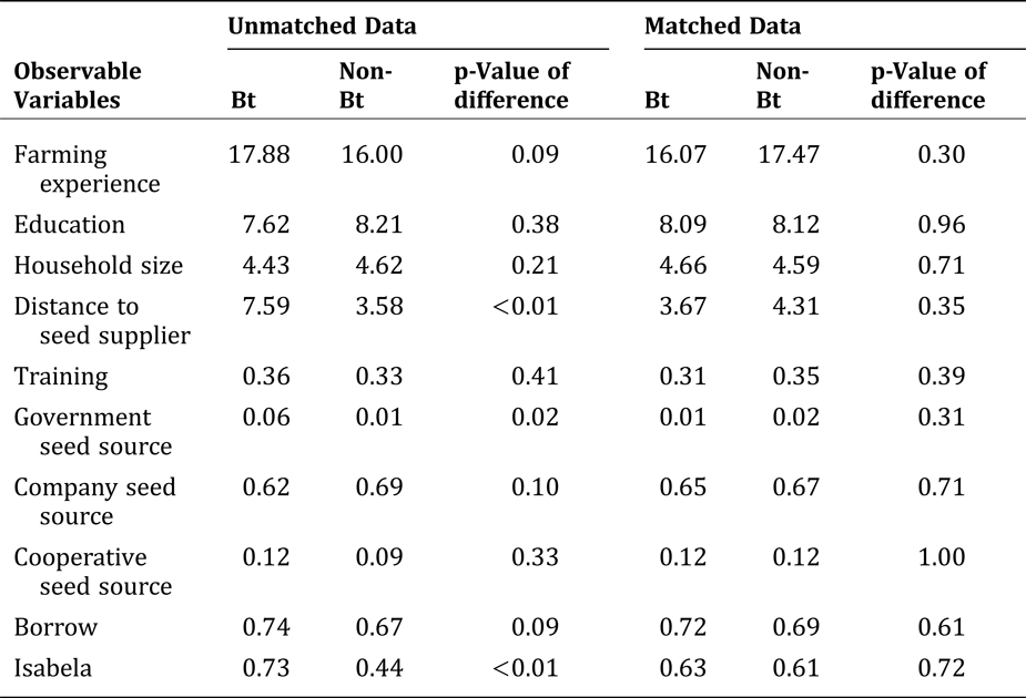
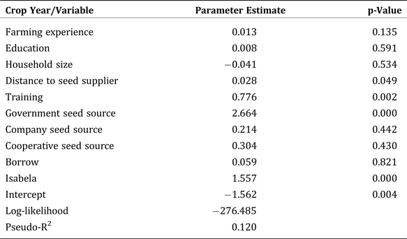
We account for these selection problems by using propensity score matching (PSM).Footnote 9 We recognize that PSM can only control for the selection problem due to observable characteristics and not for the selection problem due to unobservable characteristics. We argue, however, that if the observable characteristics (e.g., education and experience) we include in the model can already account for the unobservable characteristics (e.g., management ability), then PSM can also solve the selection problem on unobservables.Footnote 10 Ideally, the best “control” group with which to compare the performance of the Bt adopters is the group of Bt adopters themselves, had they not adopted Bt (i.e., the so-called counterfactual). However, this is unobservable because Bt adopters cannot be non-Bt adopters at the same time. Hence, nonadopters are typically used as the “proxy” counterfactual. In our PSM, logit models of Bt adoption is first estimated to generate propensity scores for Bt and non-Bt adopters. Using the estimated propensity scores, the PSM approach enables us to find matching non-Bt adopters that are “similar” to the Bt-adopters, so that valid yield (or risk) effects of Bt technology can be estimated. We include a number of independent variables as the observable characteristics in the logit adoption model to account for all possible variables that could determine adoption and yields.Footnote 11 While we wanted to include a larger number of exogenous factors as observable characteristics, such as total land area owned, soil quality, and access to irrigation, these were not included in the survey data. To ensure that the sample of the Bt adopters and the sample on non-Bt adopters have similar mean propensity scores and observables at various level of propensity scores, the balancing property of the logit specification is tested. Using the calculated propensity scores from the logit model that satisfy the balancing property, the one-to-one or pair matching without replacement is then used to match non-Bt adopters with similar propensity scores with Bt-adopters.Footnote 12 Selection and endogeneity tests are conducted on this matched sample to determine whether the selection/endogeneity issues are accounted for through PSM.
Once the parameters of the production functions are estimated using the matched sample, the welfare implications of Bt adoption is assessed using the risk premium (R) and certainty equivalent (CE) measures defined in (4) and (2), respectively. We assume that the farmer's utility is represented by a constant relative risk aversion (CRRA) utility function: U(π) = −π1−r , where r > 1 is the coefficient of relative risk aversion. We use r = 2 where U(π) = −1/π in our analysis.Footnote 13 This characterization of the utility function was chosen because it reflects risk aversion and DARA behavior (see footnote 2). The approximate risk premium (as defined in (4)) is then calculated so that the variance effect and the skewness effect of Bt can be assessed separately. The CE measure is calculated next using (2), where p is the average output price gathered from the survey, and c(x) is a vector of average input costs also calculated based on the survey data.Footnote 14
Another welfare measure considered in this study is the Lower Partial Moment (LPM) measure (see Unser Reference Unser2000). This measure only considers the lower part of the profit distribution as follows:
where π0 is the farmer's profit target, π is the farmer's profit, f(π) is the profit distribution, and m is the order of LPM (i.e., the weight placed on negative deviation from π0). We set the farmer's profit target as zero and use m = 0, which is essentially the probability of a profit loss from growing Bt or non-Bt corn.Footnote 15 To calculate (15), we used the estimates from the production function. This allows us to simulate a profit distribution (at the mean values of all inputs, output price, and costs) and then calculate the LPM in (15).
Results
Descriptive Statistics and Propensity Score Matching (PSM) Results
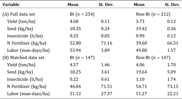
The summary statistics for the variables used in the stochastic production function estimation are presented in Table 1. For the 2007/2008 crop year, the mean yields and N fertilizer application of Bt farmers tend to be larger than those for the non-Bt farmers.
Table 1. Summary Statistics for: (A) the Full Data Set and (B) Matched Data Set (2007/2008 Crop Year)

PSM was undertaken in this study to account for possible selection issues with regards to Bt adoption. This subsample of matched Bt and non-Bt farmers are used to then estimate the stochastic production function.Footnote 16 Based on our PSM runs, there are 147 matched Bt and non-Bt observations for the 2007/2008 crop year.Footnote 17 The summary statistics for the matched sample are also presented in Table 1. Similar to the full sample, the mean yields of Bt farmers tend to be larger than those for the non-Bt farmers. However, the amount of N fertilizer applied of non-Bt farmers tend to be bigger than those for the Bt-farmers. Note also that the difference between Bt and Non-Bt farmers in terms of yield and N fertilizer application is much smaller for the matched sample than for the full sample.
Stochastic Production Function Results
In Table 2 (Panel A), the parameter estimates from our extension of the Saha et al. (Reference Saha, Shumway and Havenner1997) model are presented. The results for crop year 2007/2008 suggest that the conventional (non-damage-abating) inputs—N fertilizer and labor—have a statistically significant positive effect on mean yields, which we expected a priori.Footnote 18 To ascertain the magnitude of the impact of Bt, we calculate the marginal effects of Bt on the mean, variance, and skewness of yields (Table 2, Panel B). Given that the Bt variable is binary, the marginal effect of Bt on the mean, variance, and skewness of yields are calculated as (E(y)|Bt − E(y)|Non-Bt), (V(y)|Bt − V(y)|Non-Bt), and (S(y)|Bt − S(y)|Non-Bt), and, with all other variables held fixed at their mean values using the parameter estimates in Panel A of Table 2.Footnote 19 The marginal effects suggest that Bt has a statistically significant positive effect on mean yields (at the 10-percent level of significance). The marginal effect results also suggest that Bt has a statistically significant variance-increasing effect (at the 5-percent level of significance) and skewness-increasing effect (at the 1-percent level of significance).Footnote 20
Table 2. Parameter Estimates for the Extension of the Saha et al. (Reference Saha, Shumway and Havenner1997) Model and the Resulting Marginal Effects of Bt on the Mean, Variance, and Skewness of Yields
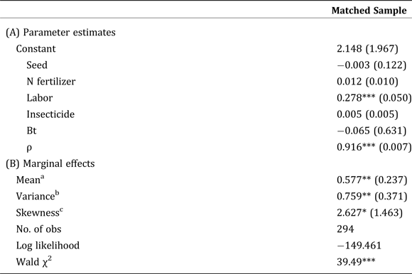
a The mean effect is calculated as: (E(y)|Bt−E(y)|Non-Bt).
b The variance effect is calculated as: (V(y)|Bt−V(y)|Non-Bt).
c The skewness effect is calculated as: (S(y)|Bt−S(y)|Non-Bt).
*, **, *** Statistically significant at the 10-percent, 5-percent, and 1-percent level, respectively.
Welfare Effects: Risk Premium, CE Estimates, and the Probability of Profit Loss
For crop year 2007/2008, our results show significant effects of Bt corn on production risks (e.g., variance and skewness of yields). In this case, there would have a statistical difference between the risk premiums of Bt farmers and non-Bt farmers. It is straightforward to infer that the strong positive mean yield effect of Bt would result in a higher CE welfare measure for Bt farmers relative to the non-Bt farmers (i.e., based on CE, Bt will be preferred). However, given that the marginal effects of the variance and skewness of yield have opposite effects, will the mean yield effect of Bt corn still overwhelm the risk effects of Bt? Will the CE estimate still be higher for Bt farmers in this case?
To answer these questions, we use the parameter estimates from Table 2 (Panel A) to calculate the second and third moments (variance and skewness) of profits, and then we compute the risk premium (R) associated with Bt and non-Bt corn.Footnote 21 The CE can then be calculated directly using R and the mean expected profit (see (2) above). The variance and skewness components of the risk premium, the total risk premium (R), and the CE for Bt and non-Bt corn are presented in Table 3. The results reveal that R is higher for Bt than non-Bt, and, in this case, the downside risk-increasing effect dominates the variance-increasing effect of Bt. Moreover, the CE for Bt corn farmers is higher than the CE of non-Bt farmers, although the difference is marginally significant at the 19-percent level. Hence, there is evidence that the Bt farmers are still better off in welfare terms than non-Bt (hybrid) producers (i.e., higher R and CE in absolute terms), but the difference may not be as pronounced. This may be because a matching approach reduces the number of observations significantly. Using a full sample (without PSM), the CE for Bt farmers is statistically higher than the CE for non-Bt farmers at the 1-percent level of significance.
Table 3. Welfare Effects of Bt Corn: Variance Effect on Risk Premium, Skewness Effect on Risk Premium, Total Risk Premium (R), and Certainty Equivalent (CE)

Note: The p-value for the test of equality of the CEs for Bt and non-Bt is 0.190 and 0.001 for matched and full samples, respectively.
For the LPM measure or the probability of profit loss from growing Bt compared to non-Bt, we simulate profit distributions using the parameter estimates from Table 2 at mean values of all inputs, output price, and costs (i.e., these means are based on the survey data). The simulated profit distributions of Bt and non-Bt farmers for the production function are presented in Figure 1. The area under the profit distribution curve to the left of zero profit is the probability of profit loss. The area under the profit distribution curve to the left of zero profit for crop year 2007/2008 is equal to 0.106 for Bt farmers, which is smaller as compared to the area of 0.128 for non-Bt farmers. We formally test for the equality of the areas under the profit distribution curve to the left of zero for the Bt farmers versus the non-Bt farmers, we find that the difference in the probability of profit loss for Bt versus non-Bt farmers is statistically significant at the 1-percent level. This implies the use of Bt corn has a reduced probability of crop loss, and Bt farmers tend to be better off. This is consistent with the R and CE results we present above.
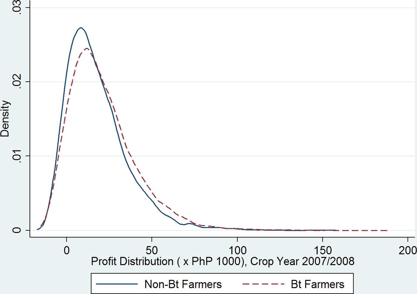
Figure 1. Simulated Profit Distribution Based on the Parameter Estimates from the Extension of the Saha et al. (Reference Saha, Shumway and Havenner1997) Model
Another profit/welfare-oriented issue that would be informative here is to determine whether the observed benefits from the mean yield effects of Bt corn compensate for the increased cost of using the Bt seed technology. It is possible that Bt increases mean yields, but the cost could have been prohibitive such that the higher Bt seed costs negate the benefits of the yield increase. Based on the mean yield effects in Table 2, as well as corn prices and seed costs from the data, we find that the estimated revenue benefits of Bt more than compensates for the increased cost of the Bt seed (Table 4). However, the net revenue above seed cost for Bt farmers (vis-à-vis non-Bt farmers) is not statistically different in 2007/2008. These results imply that the mean yield-increasing effect of Bt corn compensates for the increased cost of the seed, but the resulting net revenues may not be statistically different from the net revenues of non-Bt adopters.
Table 4. Assessment of If the Mean Yield Increasing Benefit from Bt Corn Compensates for the Higher Cost Associated with the Bt Seed Technology (Crop Year 2007/2008)

Note: (1) Corn price, seed price, and seed costs are averages based on the actual prices paid by the farmers included in the survey. All other costs are assumed equal between Bt and non-Bt farmers (only seed costs differ). (2) The p-value from test of equality in the net benefit levels of Bt versus non-Bt farmers is 0.156 and 0.001 for matched and full samples, respectively.
Conclusions
Using a stochastic production function estimation approach that allows for examining the skewness effects of Bt technology within a damage-abatement specification, this paper investigates the impact of a single-trait Bt corn technology on production risk and farmer welfare within a developing country environment. We used farm-level survey data of corn production collected in the Philippines for the 2007/2008 crop year to conduct our analyses. Propensity score matching was used to account for potential selection bias due to the nonrandom placement of Bt treatment. Results from the stochastic production function estimates indicate that Bt corn has a strong statistically significant mean yield-increasing effect, and that Bt technology significantly reduces production risk due to stronger skewness-increasing effect than the variance-increasing effect for the specific crop year under study.
In terms of the welfare effects of Bt corn, the strong mean yield-increasing and downside-risk-reducing effects of Bt corn in the Philippines imply higher certainty equivalent measures for Bt farmers than those for non-Bt farmers. Our analysis shows the mean yield-increasing effect and skewness-increasing effect of Bt corn tends to dominate the variance-increasing effect such that the magnitude of the overall welfare measure (i.e., the certainty equivalent) for Bt farmers is larger than those of non-Bt farmers. However, the higher certainty equivalents for Bt farmers over non-Bt farmers are not statistically significant. The lack of statistical difference may be due to the reduction of observations using the PSM approach. Consistent with the certainty equivalent welfare results above, we find the probability of suffering a profit loss is lower for Bt farmers than for non-Bt farmers. The lower probability of loss for Bt farmers was statistically different from the probability of loss of non-Bt farmers.
It is important to keep in mind the limitations of our analysis. First, this study only uses data from a single cross-sectional data set, rather than a panel data set. Using a panel data set in the future would enable one to better account for individual farmer heterogeneity and selection issues. A panel data analysis with more than two years of data would also provide more insights into the dynamics and evolution of production risk over time (i.e., temporal risk effects rather than cross-sectional risk effects). Second, we only focus on a particular single-trait Bt corn variety for a specific developing country. In the present study, the survey data were collected when multi-trait varieties (i.e., with multiple resistance to pests such as for borer and rootworms, as well as herbicide tolerance) were not yet widely available and adopted. As multi-trait Bt corn varieties become more widely available in the Philippines and across the globe, it would be interesting to see whether or not the risk reduction observed in experimental trials of multi-stack varieties in the United States (Shi, Chavas, and Lauer Reference Shi, Chavas and Lauer2013) can also be observed in other parts of the world—particularly in a developing country context, where smallholder farmers typically have limited options to manage risk. If these multi-stack varieties improve yields and reduce risk in developing countries, then small subsistence farmers would likely benefit more from this multi-trait Bt technology.
Third, the results of our study are greatly dependent on the crop growth conditions during the survey year (2007/2008). Note that the crop year 2007/2008 was considered a bad weather year for corn due to an extreme dry spell in Isabela province and unusually heavy rains in South Cotabato province (Yumul et al. Reference Yumul, Cruz, Dimalanta, Servando and Hilario2010). In this bad weather condition, pest infestation tends to be lower, and Bt technology tends to provide a smaller yield advantage over non-Bt varieties (See Ma and Subedi Reference Ma and Subedi2005, Shankar et al. Reference Shankar, Bennett and Moorse2007). Future work should focus on carefully examining the role of weather conditions on the yield impacts of Bt technology.
APPENDIX
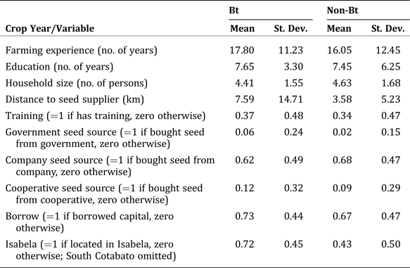
Appendix 1. Summary Statistics of the Variables used in PSM [Crop Year 2007/2008 (Bt: n = 254; Non-Bt: n = 212)]
Appendix 2. First Stage Logit Results for the PSM [Crop Year 2007/2008 (Bt: n = 254; Non-Bt: n = 212)]
Appendix 3. Comparison of Means of the Observable Characteristics for the Unmatched and Matched Data
