Antarctic precipitation and its contribution to the global sea-level budget

Abstract

Antarctic precipitation estimations derived from several new sources are examined in comparison to results found previously. The availability of analyzed atmospheric datasets has been a significant and beneficial tool for atmospheric and climate research for a broad range of research interests. This is particularly true for the polar regions, where the observational arrays are sparsely distributed. in high southern latitudes, a comprehensive assimilation of all available observations, including satellite data, is necessary for an accurate depiction of the atmospheric circulation. Recent st udies have found the operational analyses of the European Centre for Medium-range Weather Forecasts to be superior to those of other weather-forecasting centers in depicting the large-scale atmospheric circulation patterns over Antarctica. “Re-analysis” programs at major weather-forecasting centers have produced atmospheric numerical analyses using a “frozen” data-assimilation system. These projects have also derived precipitation and evaporation fields using an ensemble of short-term forecasts. From these new sources, Antarctic Ρ - E (precipitation minus evaporation/sublimation) is compared and evaluated against the long-term glaciological synthesis, as well as results from previous studies. The comparisons indicate significant regional disagreements exist between P — E from the re-analysis forecasts and the glaciological data. For the ensemble forecasting method, the continental-average evaporation is the largest area of uncertainty and differs by an order of magnitude between the rc-analysis datasets. This finding supports the use of the atmospheric moisture budget for determining P — E collectively in atmospheric diagnostic studies for Antarctica.

1 Introduction

Global sea level is an important variable with clear relevance to climate-change study (Warrick and others, 1996). Recent satellite programs, including ERS-1 and TGPEX/ Poseidon, have examined global sca-level temporal variability over limited periods of time (Nercm, 1997). An accurate appraisal of future eustatic change requires a detailed understanding of the various sca-level budget components. One of the largest areas of uncertainty is the contribution of the Antarctic ice sheet. Annual accumulation over the continent has previously been estimated to be approximately 5 mm a⁻¹ in equivalent global sea-lcvel (ESL) decrease (Fortuin and Oerlcmans, 1990). This quantity is generally restored to the sea-level budget through iceberg calving and basal melting of ice shelves. Variability in atmospheric circulation can alter ice-sheet precipitation over short time-scales, while the icc-shcet response occurs over much longer time-scales (Fortuin and Oerlemans, 1990). Investigations using global climate models (Ohmura and others, 1996; Thompson and Pollard, 1997) suggest that Greenland and Antarctic surface mass balances make opposite contributions to the present global sea-level rise, with the negative contribution of Antarctica dominating. Observational estimates of recent Antarctic precipitation variability, however, are encumbered by a variety of factors (Bromwich, 1988). Biases associated with wind-induced turbulence and the introduction of blowing snow create tremendous difficulties in using snow-gauge measurements. Glaciological measurements of accumulation are generally considered straightforward, but the available observations lack the uniform spatial and temporal resolution needed to examine the continental area. These deficiencies in surface-based measurements have led to the examination of atmospheric techniques, including assimilated datasets.

Atmospheric numerical analyses are routinely produced by operational weather-forecasting centers for the purpose of initializing short- and medium-range weather-forecasting models. The analyses incorporate all meteorological data that are available to the forecasting center, including satellite data. The archiving of these analyzed fields has produced an important tool for use in meteorological and climate study (e.g. Trenberth and Olson, 1988; Trenberth, 1992). Recent studies (Bromwich and others, 1995; Cullather and others, 1997) have shown the analyses produced by the European Centre for Medium-range Weather Forecasts (ECMWE) are superior to other analyses in depicting the large-scale circulation features and moisture budget of high southern latitudes. The atmospheric moisture budget study of Bromwich and others (1995) and other recent studies (Howarth, 1986; Masuda, 1990; Yamazaki, 1992, 1994; Budd and others, 1995) have demonstrated the viability of this method. A significant difficulty with the use of operational analyses for climate study is the fact that the analyses are produced primarily to initialize short-term forecast models. Changes are frequently made to the data-assimilation system for the improvement of the forecast model. This creates the problem of discerning spurious changes to the analysis system from real climate variability in an extended time series. in an effort to address this problem, “re-analyses” have been produced using a “frozen” data-assimilation system. in these data, either variability is a real signal of the natural atmosphere or it results from changes in the data network. The expanded datasets from the re-analyses include fields from short-term forecasts initialized using the re-analyzed initial fields.

In this paper we examine the results obtained by Cullather and others (1998) using the moisture budget of the operational ECMWF analyses, in comparison to the recently available datasets of the ECMWF and U.S. National Centers for Environmental Prediction/National Center for Atmospheric Research (NCEP/NCAR) re-analysis projects. Section 2 presents an overview of the data-sets considered in this study, as well as the moisture-budget method employed on the ECMWF operational analyses. in section 3, an assessment is made of the spatial depictions in comparison to the long-term glaciological synthesis. Section 4 presents a comparison of the annual cycles and interann-ual variability produced by each of these methods. These results are examined in the context of the Antarctic ice-sheet contribution to the global sea-level budget. Finally, section 5 presents an overview of issues related to Antarctic precipitation variability.

2 Datasets and the Atmospheric Moisture Budget

Several different types of precipitation data are available for polar ice sheets. These different variables are related via the surface budget using (Bromwich, 1988):

(1)

where angled brackets represent an areal average and the overbar represents a time average, Β is accumulation, Ρ is precipitation, E is the net of sublimation minus deposition of hoar-frost, D is the divergence of snowdrift transport and M is the divergence of melt water runoff. in estimating ice-sheet mass balance, the areal accumulation rate is balanced against iceberg calving and basal melting at the bottom of ice shelves. A review of these terms is given by Jacobs and others (1992). It should be noted that Equation (1) is somewhat idealistic in partitioning the various contributions. For example, sublimation from blowing snow may be significant. Notwithstanding, the dominant term in Equation (1) is precipitation, and, to a first order, the spatial distributions of Β, Ρ and P—E have been thought to be comparable (Bromwich, 1988), although evaporation/sublimation can be large (e.g. Stearns and Weidner, 1993).

The operational ECMWFanalyses used in lliis study are from the Tropical Oceans Global Atmosphere (TOGA) Archive II, a twice-daily global 2.5° x 2.5° dataset reported at near-surface and 14 standard pressure levels. After 1991, the dataset includes a 15th level at 925 hPa, which is omitted here for temporal continuity. The dataset is described and evaluated by Trenberth (1992). in addition to the moisture-budget study of Bromwich and others (1995), Cullather and others (1997) have evaluated the standard ECMWF and NCEP variables over Antarctica using available rawinsonde, automatic weather station, ship, and synthesized long-term observai ions. The ECMWFanalyses were generally found to be superior, and to depict reasonably the broad-scale atmospheric circulation.

From these operational ECMWFanalyses, the moisture budget was computed for the years 1985-93 using the method outlined in Cullather and others (1998). A derivation of the atmospheric moisture budget is given by Peixoto and Oort (1992) from first principles. The budget may be expressed as:

(2)

where A is the area of interest, W is precipitable water, P_sfc is surface pressure, q is specific humidity, V is the horizontal wind vector and n is the outward-pointing normal vector of the area perimeter. The variable P_top is the highest level of the atmosphere, which is not zero in the analyses. in the operational ECMWFanalyses, horizontal wind data extend to 10 hPa, while atmospheric moisture is considered negligible above 300 hPa. Equation (2) is written so that the residual is expressed as Ρ — E for comparison with glaciological accumulation. The first term on the righthand side is the time derivative of precipitable water, and is referred to as the storage term. Four adjacent gridpoints are used to define an area and boundary. The units in Equation (2) are kg m⁻²s⁻¹, which is equal to the rate of mm⁻¹s of water-equivalent precipitation.

A comprehensive review of the NCEP/NCAR re-analysis project is given by Kalnay and others (1996). The system utilizes a quality-controlled data-assimilation system and a global spectral numerical weather-prediction model withT62 horizontal resolution (approximately 1.9° x 1.9°) and 28 vertical levels. Some of the important considerations for examining the NCEP/NCAR re-analysis in high southern latitudes are outlined in Cullather and others (1998). These include the misincorporation of manually derived sea-level pressure observations over the Southern Hemisphere during the assimilation process, and a spurious spectral distortion pattern in polar moisture fields. These two errors suggest considerable caution in evaluating results over the AntarctiC. The ECMWF re-analysis project (ERA) also utilizes a refined data-assimilation system and aT106 forecast model with 31 vertical levels (Gibson and others, 1996, 1997).

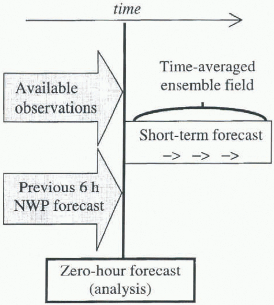
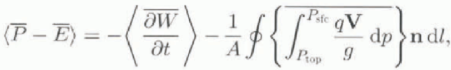
Fig. 1. Diagram indicating evolution of various weather-fore-casting-center products. Numerical analyses, from which the atmospheric moisture budget may be Computed, are produced at the zero forecast hour. Precipitation and evaporation fields are obtained from an average over some period of the short-term forecast. The procedure is repeated twice or four times daily to produce an ensemble ofanalyses and short-term fore-casts.

Fig. 2. Digitized accumulation synthesisfrom Giovinetto and Bentley (1985), plotted in units of mm w.e. a⁻¹. Spatial distribution of Ρ - E derived from (b) the atmospheric moisture budget of ECMWF operational analyses, (c) ensemble forecasts of the NCEP/NCAR reanalysis, and(d) ensembleforecasts of the ECMWF re-analysis, averaged for theyears 1985-93, plotted in units of mm w.e. a⁻¹. Contour intervals selected by Giovinetto and Bentley are used in (a), (b) and (d); a constant interval of 200 mm a⁻¹ is used in (c) for legibility.

Figure 1 is an attempt to illustrate the differences between (1) numerical analyses, from which the moisture budget may be computed, and (2) short-term forecasts, from which the average forecast precipitation field is produced. Numerical analyses are produced from the assimilation of available meteorological observations, as well as the previous 6 hour numerical weather prediction forecast, referred to as the first guess. These two sources of data are then passed through a quality-control procedure to produce the zero-hour global analysis. From the zero-hour analysis, the forecast model is then run and average precipitation and evaporation rates are computed for some part of the forecast run. The NCEP/NCAR re-analyses utilize the 0-6 hour forecast period, while the ERA uses the 12-24 hour forecast period to avoid “spin-up” in the early hours of the forecast. The procedure shown in Figure 1 is then repeated to produce numerical analyses four times daily. For a 30 day month, an ensemble of 60 short-term forecasts is used to produce the monthly-averaged precipitation and evaporation fields from the ERA.

3 Spatial Distributions

The long-term synthesis of glaciological observations is an important benchmark for comparison with new datasets. The most recent of these is the synthesis of Giovinetto and Bentley (1985), which has been used for validation in numerous studies (e.g. Tzeng and others, 1994; Connollcy and King, 1996; Ohmura and others, 1996). Two receñí studies have demonstrated local discrepancies in the climatology in the vicinity of the Antarctic Peninsula (Frölich, 1992) and Lambert Glacier (Higham and Craven, 1997). These studies suggest the need for a revised accumulation distribution for the continent, but also illustrate the problem faced when synthesizing a long-term variable for regions where values are susceptible to intcrannual variability. The Giovi-netto and Bentley climatology is the best synthesis of glaciological data currently available, however. Giovinetto and Bentley (1985) indicated an uncertainty of ± 10% in their accumulation estimate for Antarctica. This climatology has recently been produced in a digital version by its authors, which is shown in figure 2a. This digital version contains data only for the grounded ice-sheet areas, which is sufficient for this study of the eustatic impact. The field contains values at a 1° x 1 ° latitude/longitude resolution. The areal average of this field where values are available is 151 mm a⁻¹.

figure 2b shows the spatial distribution of Ρ — E derived from the atmospheric moisture budget using ECMWF operational analyses, averaged for the years 1985-93. The figure is qualitatively similar to the Giovinetto and Bentley climatology in showing essentially desert-like conditions over a large area of the East Antarctic interior surrounded by a large spatial gradient along the coasl. Larger values are present in West Antarctica, with the continent's largest values occurring along the western side of the Antarctic-Peninsula. The average of these data for the identical region used in the Giovinetto and Bentley climatology is 137 mm a⁻¹. Figure 3 presents the difference of the ECMWF moisture budget Ρ - E minus the Giovinetto and Bentley accumulation. Large regional differences are particularly noticeable in coastal regions; there are several areas where features are transposed, such as to the west and east of 30° E in Dronning Maud Land. A particularly interesting feature occurs near Porpoise Bay (~125° E) where the moisture budget exceeds accumulation by <250mma⁻¹. Near the Ross lec Shelf and West Antarctica, several regional features in the accumulation data (fig. 2a) appear to be below the resolution available to the moisture-budget method. These include the maxima along the Transanlarctic Mountains, and the minima associated with subsidence along the eastern edge of the Ross Ice Shelf and into West Antarctica, although intcrannual variability has been found to be large in this region (Cullather and others, 1996).

The distorted spatial pattern for NCEP/NCAR re-analysis Ρ has been reported by Cullather and others (1996,1998). Distortions in the Ρ -E field, shown in figure 2c, are qualitatively similar. The field is characterized by a spectral distortion pattern resulting in a variety of maxima, or bull's-eyes, scattered throughout the interior of Antarctica and into lower latitudes but mostly confined to 70° S-South Pole. The magnitude of these spatial oscillations is on the order of 400 mm a⁻¹ for the 1985-93 mean field. A similar problem has also been found in the Arctic (Scrreze and Maslanik, 1997). This is combined with a known data-assimilation problem for the inclusion of manually derived sea-level pressure observations over the Southern Hemisphere, which are substantial caveats for examining time-series results.

Fig. 3. Difference of P — E derived from the atmospheric moisture budget using ECMWF operational analyses minus Giovinetto and Bentley (1985) digitized accumulation. The contour intervals are every 50 mm a⁻¹.

figure 2d shows the corresponding P — E field from ensemble forecasts of the ERA. Superficially, the ERA-ensem-ble-forccastcd P — E spatial distribution appears to be superior to the other methods discussed here in comparison with Giovinetto and Bentley (1985). This is particularly true of the contour-parallel distribution for most of the continent, and the strong gradient along the East Antarctic coastline. A difference plot of this field with the Giovinetto and Bentley climatology, not shown, shows similar regional differences to those found using the moisture-budget method. This is particularly true of the Porpoise Bay region, along the Trans-antarctic Mountains and in West Antarctica. An exception to this is over the interior plateau, where the values are generally much less than for the accumulation field. ERA values for the highest part of the plateau are lower than those produced by the Giovinetto and Bentley synthesis by about 25 mm a⁻¹. This may be seen in figure 2d by the large area covered by the 20 mm a contour, which is absent from the Giovinetto and Bentley (1985) plot (fig. 2a).

The areal averages of Ρ — E for the grounded ice sheet are 137 mm a⁻¹ for the moisture budget from ECMWF operational analyses, 139 mm a⁻¹ for the ERA ensemble forecasts, and 161 mm a⁻¹ for the NCEP/NCAR re-analysis. All three averages are within 11 % of the glaciological synthesis value of 151 mm a⁻¹ for the grounded ice sheet. It should again be noted that contemporary data are only available from the atmospheric methods; an understanding of the discrepancies with glaciological data beyond what is presented here would require concurrent data from all methods. The comparison illustrates this limitation associated with using the long-term glaciological synthesis.

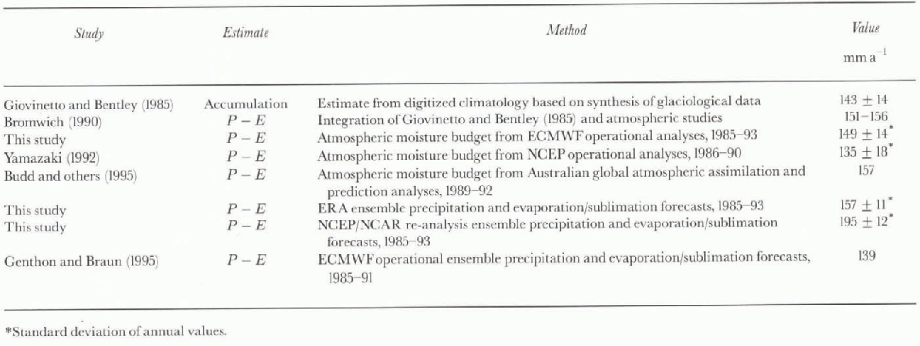
The agreement found in the average annual P — E value for Antarctica among the various methods is indicative of the general agreement found among other studies (Cullather and others, 1998). A comparison of results presented here with recent studies is shown in Table 1. The estimates are computed for an area that includes the grounded Antarctic ice sheet plus the large ice shelves. This area definition has been used as a basis for comparison in previous studies. The combined P-E estimate for the studies shown is 155 mm a⁻¹ with a standard deviation of 13%. Removing the outlying NCEP/NCAR re-analysis estimate reduces the average to 148 mm a⁻¹ with a standard deviation of 6%.

Table 1. Comparison of P- E and accumulation estimates for the Antarctic ice sheet from recent studies

4 Temporal Variability

The distribution over the annual cycle for the grounded ice sheet, shown in figure 4a, varies considerably among the datasets. There is agreement that winter values are larger than those for summer. A seasonality index computed from the ratio of winter (June August) to summer (December-February) values finds three different amplitudes, ranging from a small annual cycle for the ERA (1.4) to a larger cycle for the NCEP/NCAR rc-analysis (2.4), with the ECMWF moisture budget almost exactly in between (1.9). The discrepancies among the atmospheric methods result from estimates of evaporation/sublimation required for the ensemble model methods. This is further discussed in section 5.

figure 4b presents the annual values for Antarctica in units of mm ESL. Over the 9 year time period, the maxi-mum range for the methods estimating Ρ - E is 1.1-1.5 mm ESL a⁻¹. Both the moisture budget computed from ECMWF operational analyses and the ERA ensemble forecasts show an average value of 4.8 mm ,ESL a⁻¹, while the NCEP/ NCAR ensemble forecasts show a value of 5.6 mm ESL a . The ECMWF moisture-budget method shows a significant upward trend of 0.12 mm ESL a⁻¹ with a standard error of 0.045 mm ESL a The NCEP/NCAR re-analysis also shows a significant upward trend, with a rate of 0.07 mm E-SL a⁻¹ with a standard error of 0.05 mm ESL a⁻¹. The ERA also shows a positive trend of 0.04 mm ESL a⁻¹, but the slope is not significant in comparison to the variability. Nevertheless, a long-term increase is in agreement with available glaciological observations (e.g. Morgan and others, 1991; Bromwich and Robasky, 1993; Mosley-Thompson and others, 1995).

Fig. 4. Comparison of average annual cycle from various climatologiesfor the region specified by available data in figure 2a, averagedfir the years 1985-93, in mm a⁻¹.(b) Comparison of annual average values for various climatologies, in units of mm ESL a⁻¹.

5. Discussion

The comparison between glaciological data and time-averaged P — E value shows general convergence on a value near 150 mm a⁻¹ ± 13% for the continental average. This agreement gives confidence in validating global climate models using these long-term estimates.

The decomposition of surface accumulation rates is of particular importance to atmospheric climate modeling, which prognoses precipitation and evaporation/sublimation rates separately. This is also essential to understanding accumulation fluctuations, as climate variability may impact the terms differently (Budd and Simmonds, 1991). Unfortunately this is the source of most of the disagreement among the methods examined here. The average NCEP/NCAR re-analysis values of Ρ and E are 298 and 137 mm a⁻¹, respectively, while the ERA values are 147 and 8 mm a⁻¹. The substantial difference in evaporation/sublimation, roughly a factor of 17 between the two re-analyses, has also been noted by Stendel and Arpe (1997). The annual cycles of evaporation/sublimation are also somewhat différent. The very small number of regional observations suggests the annual cycle of evaporation/sublimation is characterized by very small or even negative (deposition) values for most of the year, with a marked increase in December and Janu-ary (e.g. Loewc, 1962; Fujii and Kusunoki, 1982; Stearns and Weidner, 1993). Not shown, the curve for evaporation/sublimation over the annual cycle in the NCEP/NCAR re-analysis has roughly the same shape as these observations but with different values; relatively small values of 110 mm a⁻¹ occur from March to October, with much larger evaporation/sublimation rates of greater than 220 mm a in summer months. in contrast, the curve for evaporation/sublimation over Antarctica in the ERA more closely resembles a sine function, with small amounts of deposition occurring from June through September. The minimum average monthly evaporation/sublimation rate of-1.8 mm a⁻¹ occurs in July, with a maximum rate of 28 mm a⁻¹ in December.

The amount of continental-averaged summer evaporation/sublimation is not presently known. Evaporation/sublimation had previously been thought to be negligible for large areas of the continental interior (e.g. Loewe, 1962), but recent observational studies from peripheral areas of the ice sheet (Fujii and Kusunoki, 1982; Faure and Buchanan, 1991; Stearns and Weidner, 1993) have found very large summer sublimation rates. These studies do not support cither of the two evaporation/sublimation fields from the re-analysis products, however, since the NCEP/NCAR re-analysis evaporation/sublimation rates are more than twice as large as the substantial values reported by Stearns and Weidner (1993); the shape of the ERA evaporation/sublimation curve raises interesting questions about the ability of observational methods to measure deposition accurately. At present, there is considerable disagreement on the separated Ρ and E terms for the Antarctic continent. This finding supports the use of the atmospheric moisture budget for determining P-E collectively in atmospheric diagnostic-studies.