Bounds on the initial macroporosity of sea ice pressure ridges

Abstract

The mass and heat balance of Arctic sea ice is affected by the deformation of level ice and the amount of ice stored in sea ice ridges and rubble fields. One important property of sea ice ridges is the macroporosity or void fraction. While macroporosity has been observed in field and laboratory studies, data are sparse and a concise theory of its evolution is lacking. In the present study, the hypothesis is investigated that the initial macroporosity of sea ice ridges is related to random loose packing. When laboratory results on the packing of ice blocks are corrected for boundary effects, good agreement with random loose packing predictions is obtained. The macroporosity then depends mainly on the length-to-thickness ratio of the ice blocks ϵ_b and it can be expected to fall in the range of $0.4 \lt \phi \lt 0.5$ for typical dimensions of ice blocks in sea ice ridges. In the field, such high macroporosity values are seldom observed., because thermodynamic adjustment, related to the increase in microporosity of submerged cold ice blocks, rapidly decreases the initial macroporosity by 0.1 to 0.15 for typical Arctic freezing conditions. Taking into account this effect, field observations are also consistent with random loose packing of ice blocks. The proposed macroporosity prediction can be useful for modeling the consolidation and property evolution of sea ice ridges and rubble fields and for improving thickness redistribution algorithms in sea ice models.

1. Introduction

The deformation process of sea ice under the influence of wind and ocean currents is often called pressure ridging: ice floes break into smaller pieces that are piling up below and above the existing ice sheet. The overall volume of deformed ice stored in Arctic sea ice ridges and rubble fields has been estimated in pan-arctic model studies to be most likely in the range of 40-60% (e.g.,Flato and Hibler, 1995; Steiner and others, 1999; Martensson and others, 2012). While pan-arctic observations are lacking, the observational range found in regional studies based on upward-looking sonar is similar (e.g.,Wadhams and Horne, 1980; Melling and Riedel, 1995; Vinje and others, 1998), underlining the important role that deformed ice plays for the Arctic mass and heat balance.¹ The major part of deformed ice is below the sea level and thus difficult to observe. Models, on the other hand, are lacking floe-scale physics of pressure ridge formation, which limits their skill to predict deformed sea ice volumes (e.g.,Flato and Hibler, 1995).

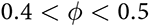
Figure 1 shows the principal model of a sea ice pressure ridge. It usually consists of a sail and a much larger keel that often have triangular or trapezoidal cross sections. The keel can be divided into a consolidated and a non-consolidated part. Sea ice pressure ridges are porous packings of ice blocks. Their nonsolid fraction, or macroporosity (contrasting the term porosity used for the air and brine pore fraction of bulk sea ice), consists of voids filled with air (when ice pieces are piled up above the water level) and seawater (when piled below). Most of our knowledge about this macroporosity is based on drilling. Zubov (1945) has reported one of the first observations of this kind obtained by Makarov in the northern Kara Sea, showing intermittent layers of water and ice in a keel determined by steam drilling. Similar historical Russian data suggested an average porosity range of 0.4–0.5 both in the keel and the sail (Burke, 1940; Doronin and Kheisin, 1975). However, the data sources and procedures of these early studies are not well documented. Later studies focused on many properties of pressure ridges, but not much on their porosity (e.g., Weeks and others, 1971). Tucker and others (1984a) developed an instrument to measure the porosity in a drill hole and reported a porosity of $0.21 \pm 0.10$ for one test. From their analysis, it became clear that many drillholes are needed to obtain an accurate porosity estimate. First detailed observations of the macroporosity of pressure ridges were reported in the 1990s for the Baltic Sea (Kankaanpää, 1988, 1997; Leppäranta and Hakala, 1992; Leppäranta and others, 1995). The key results of the studies were that (i) a ridge is consolidating faster than level ice, (ii) the rate of consolidation depends on the macroporosity of thekeel and (iii) the mechanical strength of a ridge is mainly determined by the consolidated layer. The typical macroporosity found in these studies was $\sim 0.3$ for the keel and a lower value close to $\sim 0.2$ for the sail. Strub-Klein and Sudom (2012) have summarized observations for Arctic regions, indicating similar macroporosity ranges. More recently, extensive data on the porosity of Arctic pressure ridge keels have been obtained by thermal drilling (Kharitanov, 2008, 2019, 2020a, 2021a; Guzenko and others, 2022; 2023), with average values falling mostly in the range of 0.2 to 0.4.

Most observations of the vertical distribution of macroporosity show a downward increase in the keel. Surkov (2001) has analysed Baltic sea ice ridge profiles from Kankaanpää (1997) to estimate a porosity increase from 0.29 below the consolidated layer to 0.47 in the lower part of the keel. The thermal drilling data from the Arctic show an increase in macroporosity from 0.2–0.3 below the consolidated layer to 0.3–0.4 near the bottom (Pavlov and others, 2016; Kharitanov, 2019, 2020a, 2021a; Guzenko and others, 2022, 2023). Other studies have focused on the deformation and failure criterion of ice rubble in laboratory experiments (e.g., Urroz and Ettema, 1987; Matala, 2021; Shayanfar and others, 2022). The porosity in such experiments, with block geometry chosen similar to field values, was often found in the range 0.4–0.5 and thus at the high end of field observations.

In summary, macroporosity of sea ice ridges and rubble is an important property for the engineering and sea ice modeling fields. It is difficult to observe, and only a few studies have described its spatial distribution and temporal evolution. Field and laboratory observations are not fully consistent, and there is also a lack in models to predict the macroporosity of sea ice ridges. The present study aims to close some of these gaps and develop a model for the macroporosity of rubble (the unconsolidated part of the keel, see Fig. 1) that is consistent with field and laboratory observations. The paper is structured as follows. I will first outline my basic approach and compare field and laboratory data observations of ice rubble macroporosity, including a set of new laboratory experiments. I then discuss the data with regard to theories of packing of particles and by comparison to numerical simulations of packing of ice blocks. Finally, I develop equations accounting for thermodynamic conditions that allow for the prediction of the macroporosity of rubble of known ice block salinity and temperature. The discussion presents a detailed evaluation of uncertainties and limitation of the approach and how it extends and improves related studies.

Figure 1. Typical geometry of a sea ice pressure ridge with maximum sail height H_s, maximum keel depth H_k, ice block thickness and length H_b and L_b. The ridge has partially consolidated and its consolidated layer thickness H_c is larger than the level ice thickness H_i. The void space or macroporosity ϕ in the unconsolidated part of the keel and the sail are shown in red and cyan colors (the image corresponds to ϕ ≈ 0.4 for the keel). Keel to sail proportions (4:1) are similar to observations, yet horizontal dimensions are not to scale, keel width in the field being typically 4 times the maximum keel depth, compared to a 3:2 ratio in the sketch.

2. Initial porosity of sea ice ridges—basic concept and data

In this work, I investigate the implications regarding the formation of the macroporosity of a ridge as a random particle packing problem. For spheres, the densest packing is known to be $\pi/\sqrt{18} \approx 0.7405$ and dates back to a conjecture Kepler made in the 17th century (e.g., Song and others, 2008). Two other packing bounds that have received interest by many investigators are the random dense and random loose packing. These have been shown, by experiment and theory, to be close to ≈ 0.64 and $\approx 0.55\!\!-\!\!0.56$ (Scott and Kilgour, 1969; Song and others, 2008), although their exact definition is still not completely clear. Random loose packing has been described as the “loosest possible random packing that is mechanically stable” (Onoda and Liniger, 1990).

For non-spherical particles, the packing bounds are known with less precision than for spheres. However, a couple of general aspects have emerged from theoretical, numerical and experimental studies (Zou and Yu, 1996; Delaney and others, 2011; Gan and Yu, 2020): (i) particle cohesion, or friction, produces looser packing; (ii) packing density decreases (porosity increases) with the aspect ratio of particles; and (iii) sedimentation of particles does not lead to random loose packing in a strict sense and the achieved packing is often algorithm-dependent. That said, the following main processes are regarded as essential to predict the porosity of ice rubble:

1. Fracture. What is the length to thickness ratio $\epsilon_{b} = L_{b}/H$ of ice blocks forming when an ice sheet is pushed into a ridge? The challenge is to determine the breaking length L _b in dependence on floe thickness H _b and thus understand how sea ice fractures (Sayed and Frederking, 1989; Lau and others, 2012).

2. Packing. How dense do blocks pack in dependence on their aspect ratio $\epsilon_{b}$ and shape? This may be expressed as $\phi = F (\epsilon_{b}, \text{shape, friction})$, where ϕ is the rubble porosity (related to packing fraction $\phi_{p}=(1-\phi)$). The function F is expected to depend on particle shape. For example, prolate (cylindrical) and oblate (disks) particles with the same aspect ratio will pack differently. F also depends on the question if ice blocks pack in a random loose or dense manner and hence on their cohesion and friction.

3. Thermodynamics. When cold sea ice is submerged into warmer seawater, the system must reach a new thermodynamic equilibrium. What does this imply for the ridge micro- and macrostructure?

In this study, I mostly focus on the modeling of (2) Packing and (3) Thermodynamics, yet also provide a simple empirical formula for the block aspect ratio $\epsilon_{b}$ (1).

2.1. Field data

To evaluate the potential to predict the porosity of sea ice ridges by particle packing theory, I will use the observations in Table 1. Most of these were compiled on the basis of a comprehensive overview on ridge properties by Kankaanpää (1997) and Strub-Klein and Sudom (2012). The essential observational variables to investigate the packing problem are the (unconsolidated) keel macroporosity ϕ, the block major length L _b and the block thickness H _b in a ridge. Keel macroporosities reported in three studies (Veitch and others, 1991; Leppäranta and Hakala, 1992; Kankaanpää, 1997) include the solid consolidated layer thickness H _c. In order to obtain the macroporosity of the unconsolidated part of the keel, a correction factor $H_\text{k}/(H_\text{k}-f_\text{k} H_\text{c})$ has been applied, based on keel depth H _k and consolidated layer thickness H _c. The submerged fraction of the consolidated layer was taken as $f_\text{k}= 6/7$ assuming isostasy for Baltic Sea conditions (Leppäranta and Hakala, 1992; Kankaanpää, 1997). In most sections, it is neglected that blocks have a width that is smaller than the length to keep the analysis as simple as possible and focus on the key variable – the major length to thickness ratio $\epsilon_{b}$. The influence of different width is shortly addressed in the discussion. The data in the table present an overview of ridges from different regions (Baltic sea, Arctic sea and Barents sea).

Table 1. Selected studies of macroporosity of unconsolidated rubble in sea ice ridges from the field and laboratory studies, where keel porosity ϕ, block thickness H _b, major block length L _b, aspect ratio ϵ_b and number of observations are documented. Upper: field studies with measured block dimensions in the sail; lower: laboratory studies with pre-cracked pieces. The data from Guzenko and others (2022, 2023) for five different Arctic regions are from two publications: block dimensions from 2022, macroporosity from 2023. Guzenko and others (2023) presented the average macroporosity for large and small ridges and the values given here are averages of these two numbers. Low values of 0.1 from one ridge studied by Hoyland (2007) were omitted, as the ridge contained very soft ice, for which the macroporosity is difficult to obtain. The macroporosity given by Veitch and others (1991), Kankaanpää (1997) and Leppäranta and Hakala (1992) includes the solid consolidated layer, which was corrected (see text).

2.2. Laboratory data

The laboratory data in Table 1 are based on studies with pre-cracked ice pieces. I include one study on the shear properties and behavior of rubble by Urroz and Ettema (1987) and note that there have been quite a number of such investigations, with documented rubble porosity and block dimensions. However, I am only aware of two studies where the dependence of the porosity on block aspect ratio has been investigated in detail. The first study of this type is by Surkov and others (1997). These authors cut smaller pieces of different length to thickness ratio from sea ice harvested in the sea of Okhotsk and put these randomly into metal boxes of 0.4³ to $0.75^3\,\mathrm{m}^3$ volume. The boxes were then filled up with water to estimate the macroporosity ϕ. The authors then proposed the empirical relationship

(1)\begin{equation}\phi=0.09\;\text{ln}(64.7L_b/H_b)\end{equation}

that relates macroporosity ϕ to the ratio of block length L _b to block thickness H _b in a ridge. This equation is based on laboratory experiments and has not been validated for field conditions. However, for block length to thickness ratios observed in the field (Tucker and others, 1984b; Kankaanpää, 1997), it predicts a macroporosity of 0.44–0.50, at the higher end of observations.

The new data presented here stem from a laboratory study performed by Pustogvar, motivated by the results by Surkov and others (1997). In contrast to their approach, putting ice pieces dry into a box, the method was to submerge a known number (and volume) of ice blocks piece-wise into a transparent cylindrical laboratory container in a cold room (diameter 0.4–0.6 m). Based on observations of the ice–water interface around the cylinder, a 3D-model of the volume filled by ice was then constructed (Fig. 2) and the porosity was determined from the ratio of ice to filled container volume. Floe thickness and tank dimensions were roughly scaled by 1:100 with respect to natural sea ice ridges.

Figure 2. (a) Experimental setup in laboratory experiments to form ridges from small ice blocks (thickness 6 mm, average length 2–12 cm). Ice blocks are pushed on a wooden plate into an opening and moved down a slope (not visible) into the small artificial ridge; (b) 3D constructing of the known volume filled by a known number ice blocks, from which the macroporosity was computed (axis units are centimers).

3. Particle packing

3.1. Correlations based on sphericity

I now turn to the first point noted above – a general model of the packing density of particles in dependence on their aspect ratio, to which one can compare the sea ice observations. While random packing of objects, in particular spheres, has been studied by many investigators, there are little studies on random packings of cubes or square cylinders. As pointed out by Jiao and Torquato (2011), cubes have the ability to fill all the space, such that the results depend on the packing algorithm. Zou and Yu (1996) developed a packing model for non-spherical particles on the basis of the knowledge about spherical particles. This model generalizes the packing behavior of particles into prolate and oblate classes and gives for each class the loose and dense packing bounds in terms of sphericity. Sphericity S _p is defined as the inverse ratio of the surface area of a particle to the surface area of a sphere with equal volume. Let A _p be the surface area of a particle and V _p the volume, then S _p is

(2)\begin{equation} S_{p} = \pi^{1/3} \frac{\left(6 V_{p} \right)^{2/3}}{A_{p}}. \end{equation}

For sea ice, the problem may be restricted to the case of oblate, disk-like particles. For this class, Zou and Yu (1996) have developed the following empirical relationships between porosity and sphericity:

(3)\begin{equation} \phi = \text{exp}\left(S_{p}^{0.6} \text{exp}\left(0.23 \left(1-S_{p}\right)^{0.45}\right) \text{ln}\left(0.40\right)\right) \end{equation}

for loose packing and

(4)\begin{equation} \phi = \text{exp}\left(S_{p}^{0.63} \text{exp}\left(0.64 \left(1-S_{p}\right)^{0.54}\right) \text{ln}\left(0.36\right)\right) \end{equation}

for dense packing. These carefully evaluated relationships may not be applicable to all shapes, yet capture the behavior of disk-like particles very well. Seckendorff and Hinrichsen (2021) have reviewed other relationships. As discussed in more detail later, sea ice blocks in ridges have a similar plate-like geometry, and one can expect that similar scalings are applicable to the packing of sea ice floes.

In Fig. 3, loose and dense random packing of disks as predicted by Eqs. 3 and 4 from Zou and Yu (1996) are compared to the field and laboratory observations of ridge and rubble macroporosity. Also shown is the laboratory-based empirical fit obtained by Surkov and others (1997) for their data. The laboratory data in Fig. 3b agree reasonably with the results from Surkov and others (1997) as well as their empirical relationship and extend the data range to higher block aspect ratios. However, most data fall clearly above the loose packing limit from Zou and Yu (1996). Only the observations from Urroz and Ettema (1987) fall between the loose and dense packing limits. These, however, show considerable scatter.

Figure 3. Comparison of (a) field and (b) laboratory observations of macroporosity versus ice block length to thickness ratio. Shown are the loose and dense packing prediction by Zou and Yu (1996), Eqs. 3 and 4, and the laboratory-based empirical fit from Surkov and others (1997), Eq. 1.

The field data in Fig. 3a show ridge porosities that are 0.1–0.3 lower than the laboratory observations. Many macroporosity data points, especially those from Baltic Sea ice ridges, fall below the dense packing limit. At first glance neither field and laboratory observations of macroporosity appear comparable, nor does it seem that random packing approximations are applicable to field data that shows large variability.

3.2. 3D numerical simulations

The macroporosity in laboratory experiments is slightly above the loose packing limit. Such a result is consistent with results for other materials. Many studies of different granular media have found that the porosity may be biased high when the container diameter or height is not sufficiently large compared to the particle dimension (Mueller, 1992; Zou and Yu, 1995; Theuerkauf and others, 2006).

To investigate this aspect, I have performed 3D simulations of particle packing with GeoDict (GrainGeo, 2021), using the software package PileGeo. It allows to digitally pile 3D particles of defined size and shape into a container. Particles are generated randomly on the input plane of the container from where they fall vertically until they settle. The piling algorithm in GeoDict does not allow for specifying friction, but seeks for the most stable position of a particle within a defined distance from the position to which it first settles, by testing a specified number of shifts, maximum shift angle, rotations and maximum rotation angle. Details and validation procedures are given in Appendix A.

In Fig. 4, results from packing simulations of a rubble pile of blocks with length to thickness ratio 4 are shown, with the final 3D result in (a) and average porosity profiles in the horizontal and vertical directions in (b) and (c). In the vertical profile one observes three boundary effects: (i) opposite to the input plane where particles start packing (in the figure to the right), there is a wavy pattern with a wave length of the order of the block thickness H _b (20 voxels in the simulation). This pattern does not create a net effect on the average porosity. At the input plane (bottom in Fig. 4a), however, one finds two boundary layer effects: (ii) at the very bottom, there is a very high porosity layer, with ϕ close to one, of half the floe thickness H _b (here 10 voxels) and (iii) near the bottom and just above layer (ii) one finds a boundary layer of half the flow length L_b (20 voxels), wherein the solid fraction ϕ_p increases from zero to the infinite packing limit $\phi_{p0}$. These layers are most clearly seen in Fig. 4c.

Figure 4. Overview of results of packing simulations with GrainGeo (2021). (a) 3D image of packed blocks with a length to thickness ratio of 4, and ice plates are shown in white and water in red; (b) horizontal average solid fraction profile and (c) the vertical average solid fraction profile (input plane on the left). The boundary layer with high porosity is visible in (a) and quantified in (c). Block thickness and length in the simulations were 20 and 80 voxel units, respectively.

In the 3D images, the boundary layer effect is readily removed by cropping the bottom regime and I found that effects (ii) and (iii) may be approximated as

(5)\begin{equation} \phi_{bl} = \phi_{0} + \left(1-\phi_0\right)\left(\frac{L_{b}}{4H} + \frac{H_{b}}{2H}\right), \end{equation}

where L _b and H _b are block length and thickness and H is the container height. In the following, this equation will be used to evaluate the observed macroporosity $\phi_{\text{bl}}$ obtained in laboratory experiments and determine the boundary-corrected ϕ ₀.

In Fig. 5a, the simulated macroporosity is compared with and without removing the boundary part. While the trend in the numerical simulations agrees well with Eq. 3 for loose packing, simulated porosities are larger, also after applying the boundary layer correction. This difference is likely related to aspects of the GeoDict packing algorithm and will be discussed further below. The important result for the moment is that one can apply Eq. 5 to correct the laboratory observations. In Fig. 5b, I show the laboratory-based macroporosities, when corrected by Eq. 5 using the experimental values of H_b and L_b, with H considered as the average filling depth as shown in Fig. 2. Now, it turns out that the laboratory-based macroporosities correspond well to the empirical random loose packing bound from Zou and Yu (1996).

Figure 5. (a) Numerical simulation results of macroporosity versus block length to thickness ratio for disks and square plates. Full symbols show results including the low porosity boundary regime, for open symbols the latter has been removed (disk and square results are shown with a small offset for better visibility); (b) macroporosity in the laboratory experiments (Pustogvar) with pre-cut ice blocks, also emphasizing the difference in results with and without the boundary layer correction (Eq. 5). The light gray shading shows the difference between the sphericity-based predictions for disks and square plates (lower and upper curves, respectively) from Zou and Yu (1996).

From other packing studies, it is known that one often finds a lateral boundary effect, with increasing porosity at the side wall of a container (Seckendorff and Hinrichsen, 2021). The constant horizontal profile in Fig. 4(b) shows that this effect is absent in the numerical simulations, which is likely due to the boundary conditions in PileGeo. The simplest approach to estimate the sidewall effect in the laboratory experiments is a linear model of the form

(6)\begin{equation} \phi_{\text{side}} - \phi_{0} \approx c_\text{s} \frac{D_{\text{eff}}}{D}, \end{equation}

where D _eff is an effective particle diameter, D the diameter of the container and c_s a factor often in the range 0.2–0.3 (Seckendorff and Hinrichsen, 2021). For the present experiments (container diameter D of 0.4–0.6 m, Table 1), estimating $D_{\text{eff}} = (L_{b} H_{b})^{1/2}$ from ice block dimensions leads to a further porosity correction of less than 0.01. As the details of experiments by Surkov and others (1997) are unknown, similar corrections cannot be calculated. However, taking the average of the ranges in tank dimension (0.4–0.75 m), ice block length (0.06–0.20 m) and block aspect ratios (1–5) reported by Surkov and others (1997), one can estimate typical porosity corrections of 0.05 for the bottom boundary effect (Eq. 5) and 0.03 for the sidewall effect (Eq. 6). With such corrections, the observations from Surkov and others (1997) would also agree reasonably with the random loose packing formula (Eq. 3).

4. Field macroporosity: thermodynamics and fracture

While the laboratory test data, after applying the boundary layer correction, turn out to be close to the loose random packing, the field data remain far off, even below the dense packing bound. With a boundary layer correction to the field data, this difference would even increase. What can be the reason for this finding? The key ideas to explain this discrepancy, outlined in the following, are thermodynamic changes during the ridge formation: When cold ice blocks are submerged into much warmer seawater, they have to adjust to a new thermodynamic equilibrium, which affects the porosity within and between the ice blocks.

4.1. Thermodynamic adjustment and micro-macroporosity exchange

To illustrate the problem, consider a sea ice block with temperature ${T_i}$ and salinity S_i and approximate its brine volume fraction by the relationship

(7)\begin{equation} v_{b} \approx -c_\text{m} \frac{S_i}{T_i}, \end{equation}

where I have chosen the variable name v _b for the microporosity (or brine volume) to avoid confusion with the macroporosity ϕ. This simplified equation for the brine volume (neglecting ice-brine density differences and the nonlinear freezing point depression) suffices for the following first estimates and the limited temperature and salinity range considered.² It is now assumed that the submerged ice block equilibrates to the seawater temperature, while keeping its salinity. This leads to a change in brine volume fraction (or microporosity), as now the internal brine concentration is higher than the equilibrium salt concentration at the seawater freezing point. When the new temperature is reached, the porosity of the ice blocks will be increased by

(8)\begin{equation} \Delta v_{b} = v_{{b}1} - v_{{b}0} \approx -c_\text{m} S_i \left(\frac{1}{T_{i1}} - \frac{1}{T_{i0}}\right). \end{equation}

To put some realistic numbers, assume $S_i = 6$ ppt, $T_{i0} = -6^{\circ}\mathrm{C}$ and $T_{i1} = -1.9^{\circ}\mathrm{C}$, then the microporosity will change from $v_{{b}0}=0.051$ to $v_{{b}1}=0.156$ and hence by $\Delta v_{b} \approx 0.105$. For this internal melting, the ice blocks will need to draw latent heat from the surrounding seawater. If the water is at its freezing point, then the ice blocks can be expected to grow on their outside and fill the macroscopic void space. This, in turn, implies a decrease in the macroporosity ϕ. In addition to their latent heat change, the ice blocks need to draw heat for their temperature increase. The enthalpy budget³ of the ridge with macroporosity fraction ϕ, ice block fraction $(1-\phi)$ and brine volume v _b of ice blocks may be written as

(9)\begin{equation} \phi_1 + \left(1-\phi_1 \right)v_{{b}1} = \phi_0 + \left(1-\phi_0 \right)\left(v_{{b}0} - \frac{c_i(T_{i1}-T_{i0})}{L_\text{f}}\right), \end{equation}

where ϕ ₀ is the macroporosity after the mechanical packing, and ϕ ₁ after the thermodynamic adjustment from $T_{i0}$ to $T_{i1}$; $v_{{b}0}$ and $v_{{b}1}$ are the corresponding microporosities of the sea ice blocks; c_i and L _f are the specific heat capacity and latent heat of fusion of pure ice. Eq. 9 states that the total porosity prior and after thermodynamic adjustment remains the same, with a slight correction related to the transition of specific heat to latent heat and phase change. This transition term may be illustrated for the above temperature example $T_{i0} = -6^{\circ}\mathrm{C}$ and $T_{i1} = -1.9^{\circ}\mathrm{C}$ by setting the salinity to zero and hence $v_{{b}0}$ and $v_{{b}1}$ to zero. Then, assuming $\phi_0 = 0.5$ and $L_\text{f}/c_i \approx 160^{\circ}\mathrm{C}$, one obtains $\phi_0 - \phi_1 \approx 0.026$.

Writing the left hand side of Eq. 9 in the form

(10)\begin{equation} \phi_1 + \left(1-\phi_1 \right)v_{{b}1} = \phi_1(1-v_{{b}1})+ v_{{b}1}, \end{equation}

one can rewrite Eq. 9 to obtain the following expression for ϕ ₁:

(11)\begin{equation} \phi_1 = \frac{\phi_0 + \left(1-\phi_0 \right)\left(v_{{b}0} - \frac{c_i(T_{i1}-T_{i0})}{L_\text{f}}\right) - v_{{b}1}}{\left(1-v_{{b}1} \right)}. \end{equation}

This equation gives the macroporosity ϕ ₁ after thermodynamic equilibrium in a ridge, originally packed with ϕ ₀, has been reached. For the example given above, $S_i = 6$ ppt, $T_{i0} = -6^{\circ}\mathrm{C}$ and $T_{if} = -1.9^{\circ}\mathrm{C}$, with $v_{{b}0}=0.051$ to $v_{{b}1}=0.156$, and a typical packing porosity of $\phi_0 \approx 0.45$ one obtains $\phi_1 \approx 0.36$ and thus a decrease in the macroporosity by 0.09. These simple computations demonstrate that thermodynamic adjustment, leading to an exchange of microporosity against macroporosity, can reasonably explain the difference between packing-based macroporosity and its actual value in sea ice ridges. Note that in the laboratory experiments discussed above, Figs. 3b and 5, only the volume of blocks filling a box was evaluated, and thus only the macroporosity without thermodynamic adjustment.

For the above estimates, a constant ice temperature was assumed, while under natural conditions, the temperature in an ice sheet varies. For a more accurate evaluation, one has to perform the calculations by averaging the brine volume, not the temperature. In the following, this was done by assuming a linear temperature gradient in the ice blocks prior to their submersion in the seawater, and the brine volume change was obtained by integration of the equations from Cox and Weeks (1983) for seawater and Leppäranta and Manninen (1988) for brackish water. Results are shown in Fig. 6a and b, where the observations are separated into the Arctic and the Baltic Sea. The reason to do so is that not only ice salinities and seawater freezing temperatures but also atmospheric temperatures are different. Focusing first on the Arctic in Fig. 6a, the results are shown for a typical ridged ice salinity range of 6–10 and ice surface temperatures of −5 and $-15^{\circ}\mathrm{C}$, a freezing point of $T_{\text{if}} = -1.9^{\circ}\mathrm{C}$ and a corresponding seawater salinity of 34.8. This represents typical warm and cold Arctic conditions and salinity ranges of thin saline ice to be ridged. The uppermost curve shows the porosity of the loose packing ϕ ₀ (the dense packing is no longer shown). The curves below show how the macroporosity changes for different ice block temperatures and salinities. It is seen that the macroporosity observations fall reasonably within the range of predictions based on typical temperature and salinity conditions. The bold upper curve can be interpreted as the packing limit for warm ice. The high porosity point in Fig. 6a, representing the warm ridge from Hoyland (2007), is consistent with this upper bound.

Figure 6. Comparison of macroporosity of the unconsolidated part of ridges from the (a) Arctic and (b) the Baltic Sea. The upper bold curves are the loose packing prediction, while all other curves give the macroporosity after thermodynamic adjustment. (a) Arctic results are shown for two ice surface temperatures −5 and $-15^{\circ}\mathrm{C}$ (emphasized by different shadings) and three ice block salinities $S_i = 6, 8 , 10$ (noted at the curves). Seawater salinity and freezing temperature are assumed to be 34.8 and $-1.9^{\circ}\mathrm{C}$. The observation (0.30) from Coon and others (1995) was taken as the mean between hard ice only (0.25) and including soft ice (0.35). (b) For Baltic Sea ridges assume more moderate ice surface temperatures −2 and $-10^{\circ}\mathrm{C}$ and three ice block salinities $S_i = 0.6, 0.8, 1.0$, with brackish water salinity and freezing temperature of 3.5 and $-0.19^{\circ}\mathrm{C}$. Note that porosities reported in three studies (Veitch and others, 1991; Leppäranta and Hakala, 1992; Kankaanpää, 1997) include the consolidated layer thickness, which has been corrected to reflect only the unconsolidated part of the keel. The three values around 0.3 at an aspect of 4.3 are for the same ridge visited three times (Leppäranta and others, 1995).

For the Baltic sea ridges, Fig. 6b, I have chosen conditions representative for the Bay of Bothnia ( $S_i = 0.6-1.0$, surface temperature $T_{\text{is}} = -2$ to $-10^{\circ}\mathrm{C}$, a brackish water salinity of 3.5 and $T_{\text{if}} = -0.19^{\circ}\mathrm{C}$), as most ridge observations are from this area. Also here the lowermost curves correspond to higher salinity, typical for rapidly growing young ice in the Baltic (e.g., Granskog and others, 2006). The agreement of observed macroporosity with the predicted range is similar to that for the Arctic region. Note that the computations for typical Baltic Sea conditions with high salinity show a stronger thermodynamic correction (decrease in macroporosity) than for the Arctic and that the observed macroporosity also shows lower values.

4.2. The role of block aspect ratio and fracture

The random loose packing algorithm requires as input the ice block length to thickness ratio $\epsilon_{b}$. Several authors have explored the relationship between ice block length and thickness (e.g., Tucker and others, 1984b; Sayed and Frederking, 1989; Kankaanpää, 1997; Lau and others, 2012). A frequently proposed approach is to consider that failure of a floating ice sheet will lead to block lengths L _b that are proportional to the characteristic length L_c of an ice sheet, known as

(12)\begin{equation} L_{b}~ \propto~ L_\text{c} = \left( \frac{E H_{b}^3}{12\left(1-\nu^2\right)g\rho_\text{w}}\right)^{1/4}, \end{equation}

where E is the elastic modulus of sea ice, ν Poisson’s ratio, $\rho_\text{w}$ seawater density and g gravity acceleration. The variation in the latter three properties may be neglected. Neglecting also the dependence on E, one obtains

(13)\begin{equation} L_{b}~ \propto~ H_{b}^{3/4}. \end{equation}

Many observations of ice block dimensions have been found to be consistent with such an assumption. Tucker and others (1984b) demonstrated this for a wide range of ice thicknesses in the Beaufort Sea and obtained from least square fitting $L_{b} = 2.85 H^{3/4}$, while Kankaanpää (1997) derived $L_{b} = 3.04 H^{3/4}$ for Baltic sea ridges. A reasonable prediction for the aspect ratio is then

(14)\begin{equation} \epsilon_{b} \approx 3.0 H_{b}^{-1/4}. \end{equation}

The presented data are also consistent with this equation. For example, based on the range of 0.11–0.87 m for H _b in Table 1 one would, using Eq. 14, estimate an aspect ratio range $3 \lt \epsilon_{b} \lt 5$, which compares to the observational range $2 \lt \epsilon_{b} \lt 7$. Numerical simulations of fracture during bending and buckling indicate a very similar range in aspect ratios (e.g., Ranta and others, 2018).

5. Discussion

In the present study, I have analyzed observations of the macroporosity of sea ice ridges with respect to the question if these can be predicted by the theory of random loose packing. I have compared theoretical predictions to field and laboratory observations of macroporosity, for which block dimensions (thickness and length) are also available. The first impression in Fig. 3 was that neither laboratory nor field observations agree with the theory. After considering finite size effects on the basis of packing simulations, good agreement of the predicted macroporosity with laboratory experiments was obtained (Fig. 5). For the field observations, I have derived a porosity adjustment that is expected after submersion of cold ice blocks in warmer seawater. The thermodynamic adjustment implies a decrease in macroporosity of a ridge on the expense of microporosity increase of ice blocks. Applying Eq. 11 with reasonable assumptions for the range of ice temperatures, ice salinity and seawater freezing temperatures, one obtains reasonable agreement of the observed macroporosity with the random loose packing bound as represented by Eq. 3. In the following discussion, I will focus on four aspects to shed more light on the quantitative skill of the model approach: (i) uncertainties related to model properties and parameters, (ii) uncertainties related to observations of macroporosity of ridges, (iii) related studies and (iv) potential model limitations.

5.1. Uncertainties related to model properties and parameters

The main uncertainties in the model relate to salinity and temperature, the ice block geometry, the time scale of thermodynamic adjustment and the potential oceanic heat fluxes. The most important points of their discussion given below are, in brief, (i) while temperature and salinity have a similar impact on predicted macroporosity, it is important to employ normalised salinities (by the seawater values) for proper model predictions; (ii) block geometry plays some but probably a minor role; (iii) the timescale of thermodynamic adjustment is less than a day for ridges that consist of moderately thin (up to $\sim 0.7$ m) ice blocks and (iv) oceanic heat fluxes do not play a relevant role in the energy budget of the early phase of ridge formation and thermodynamic adjustment.

5.1.1. Salinity and temperature

The macroporosity decrease is related to the increase in the block microporosity (Eq. 8) and thus depends on the salinity and temperature of ice blocks that form the ridge. The salinity range of 6–10 in Fig. 6a corresponds to observations of the salinity of young ice with an ice thickness of 0.3 m (e.g., Cox and Weeks, 1974; Kovacs, 1996). With a freezing point of $-1.9^{\circ}\mathrm{C}$ and seawater salinity of $S_\text{w} = 34.8$, this corresponds to a relative salinity range of $0.17 \lt S_i/S_\text{w} \lt 0.29$. To produce Fig. 6b for Baltic Sea brackish water ( $T_\text{f} = -0.19^{\circ}\mathrm{C}$, $S_\text{w} = 3.5$), the same relative salinity range has been chosen, which is reasonable for the Bay of Bothnia (e.g., Leppäranta and others, 1995). The temperatures in Fig. 6a reflect warm ( $-5^{\circ}\mathrm{C}$) and cold ( $-15^{\circ}\mathrm{C}$) ice surface temperatures in the Arctic, although more extreme values are possible. For the Baltic Sea, a more moderate ice surface temperature range (−2 to $-10^{\circ}\mathrm{C}$) was chosen.

The higher end of the assumed ice salinity range 8–10 has, while realistic for thin ice of 0.2–0.5 m thickness, rarely been reported for ridge keel ice blocks. This may be explained as follows for the different parts of the keel. First, for the consolidated part, the freezing front has passed a second time through the ice and will likely create a new equilibrium salinity for slower freezing (than for the blocks). Second, in terms of the ice blocks below the consolidated layer, the proposed thermodynamic adjustment will transform them into blocks of high microporosity. From such ice, one can expect high brine drainage during sampling and thus an underestimate of the in situ salinity. Observations of ice block density in the range 860–890 $\mathrm{kgm}^{-3}$ (e.g., Leppäranta and Hakala, 1992; Kankaanpää, 1997; Hoyland, 2007) support such salinity loss. Leppäranta and others (1995) even noted that air bubbles due to diver’s breath could go trough several ice blocks in the keel. Laboratory experiments with submerged ice blocks, where the salinity decreased while air porosity increased (Bailey and others, 2015), also support this view.

An interesting result of Fig. 6 is that the model predicts a somewhat stronger change in the macroporosity for the Baltic Sea compared to the Arctic, even though the temperatures are assumed higher. This is explained by the fact that microporosity scales reciprocally with temperature (Eq. 8), which implies a larger change in the Baltic Sea with a 10 times higher freezing point. The salinity thus plays a more important role in the macroporosity change in the Baltic Sea—the warm and cold temperature regimes overlap in Fig. 6b. It should be noted that, when considering Arctic Seas with intermediate seawater salinities, one should apply the same relative ice salinity range (e.g., for a sea with $S_\text{w} \approx 28$ the ice salinity range from 5 to 8 rather than from 6 to 10), resulting in a similar macroporosity range as in Fig. 6a.

In the Arctic field data, there are two observations of high macroporosity close to the loose packing prediction. One of these is a ridge for which Hoyland (2007) has reported that it probably formed from very warm ice with a temperature close to the freezing point of seawater. The second data point is from the study by Bonath and others (2018). However, the latter authors have estimated the age of the high porosity ridge by analysis of ice drift tracks, temperature and wind forcing, suggesting rather cold formation conditions, not consistent with the high porosity point in Fig. 6a. The only Arctic data point for which the ridge formation conditions are reasonably known is from the study by Coon and others (1995). These authors report an ice temperature of $-9.4^{\circ}\mathrm{C}$ at a depth of 15 cm in the consolidated part of a young ridge, which appears to be consistent with the cold formation condition expected from the location of their data point in Fig. 6a. For the Baltic sea, the spread is larger. The highest porosities refer to a shallow ridge from Kankaanpää (1997) and are the most uncertain because these were corrected for a consolidated layer that reached half of the keel depth. One ridge from Leppäranta and others (1995), visited several times during winter, shown with three diamonds at the same aspect ratio, formed under cold conditions, which is consistent with Fig. 6b. Given the unknown formation conditions of most ridges, the overall agreement between model and observations is reasonable.

In Fig. 7, the model approach is summarized by choosing settings considered typical for young ridged Arctic sea ice (aspect ratio of 4, ice salinity $S_i = 8$, $T_\text{f} = -1.9^{\circ}\mathrm{C}$, $S_\text{w} = 34.8$). The figure highlights how the changes in micro- and macroporosity depend on the ice surface temperature during ridging, as well as the total porosity. The microposity is computed as a porosity average over an ice block with a linear vertical temperature gradient and constant salinity. Right after ridge formation, ϕ ₀ does not depend on temperature, yet v _b0 and ϕ_t do so. After thermodynamic adjustment (about a day later), v _b1 does not depend on initial temperature, yet ϕ ₀ and ϕ ₁ are lower the lower the ice temperature initially had been. For warm ice, when the ice temperature is close to the freezing point, no thermodynamic adjustment takes place, the total porosity of the ridge keel is above 0.5 and all porosity metrics remain unchanged. Note that for cold ice, the total porosity is smaller, both initially and after thermodynamic adjustment, with its decrease given by the specific heat term in Eq. 11.

Figure 7. Predicted average macro- and microporosity ϕ and v_b and total porosity ϕ_t change during thermodynamic adjustment, for a pressure ridge keel forming from ice blocks with a length to thickness ratio of 4 and salinity $S_i = 8$ in water at the freezing point of $T_f = -1.9^{\circ}\mathrm{C}$ ( $S_w = 34.8$). The initial macroporosity from random loose packing is $\phi_0 \approx 0.44$, shown as upper solid line. The macroporosity ϕ ₁ after thermodynamic adjustment (after the ridge has reached the freezing point $-1.9^{\circ}\mathrm{C}$) is shown as the solid curve (lower bound of the dark grey shaded area) in dependence on initial ice surface temperature. The corresponding increase in the microporosity of ice blocks from $v_{b0}$ to $v_{b1}$ is shown as the lower hatched area between stippled curves, reaching $v_{b1} = 0.21$ after thermodynamic adjustment. Note that $v_{b0}$ is computed by averaging over the brine volume profile, assuming a linear temperature gradient in the ice blocks prior to ridging. The total porosity, shown with dashed curves, is computed as $\phi_{t} = \phi + (1-\phi)v_{b}$.

5.1.2. Aspect ratio and ice block geometry

In Fig. 5a, the numerical simulations with GeoDict were compared with the empirical formula from Zou and Yu (1996). While both show a similar trend, the simulated porosities are 0.05–0.08 smaller. This is not unexpected, as discussed by Seckendorff and Hinrichsen (2021), because true random loose packing is usually not realized in particle drop experiments. Geodict, however, appears to simulate this idealized state. The simulated solid fraction at an aspect ratio of 1 is consistent with the random loose packing of spheres noted above ( $\phi_{p} \approx 0.056$ or ϕ ≈ 0.044). While the empirical formula from Zou and Yu (1996) agrees better with laboratory packing experiments, including sea ice rubble, the numerical simulations allow us to study some details, like the effects of particle shape and boundaries. In Fig. 5a, the difference between square plates and disks is shown for the empirical and numerical model. The formula from Zou and Yu (1996) only predicts a difference of 0.01 for the loose packing of plates and disks, due to the difference in their sphericity. The numerical simulations show that one can expect a larger difference between the disks and square plates and that it increases with aspect ratio, where the difference is approximately 0.03 for ϵ = 4.

The blocks in a sea ice ridge are not idealized square plates of a single length to thickness ratio, but may have different shapes and consist of blocks of different size. For example, several authors have described that blocks in ridges have a length (L _b) to width (W _b) ratio close to 3/2 (Veitch and others, 1991; Kankaanpää, 1997; Strub-Klein and Sudom, 2012; Guzenko and others, 2022), while Kankaanpää (1997) noted that block shapes are not simply rectangular. To study these differences, additional numerical simulations have been performed and are compared in Table 2. Also shown is the (small) effect of the empirical prediction due to sphericity differences. The numerical simulations show (i) a higher porosity for packing of quadratic blocks compared to disks with the same aspect ratio; (ii) a slightly higher porosity for a uniform distribution of aspect ratios and (iii) a smaller porosity for rectangular blocks with a horizontal aspect of 3:2. Accounting for such details will change the porosity prediction by a few percent, falling in the range 0.49–0.53 for an aspect ratio of 4. For natural sea ice ridges, effects (ii) and (iii) will likely cancel to some degree. The problem can thus be reasonably approximated by square plates of a fixed aspect ratio.

Table 2. Random loose packing porosities predicted by Eq. 3 from Zou and Yu (1996), based on average particle sphericity, as well as the presented numerical simulations with GrainGeo (2021). The repeatability of the numerical simulations is ≈ 0.004.

While the porosity observations are limited, they show some consistency with the derived increase in macroporosity with aspect ratio, in particular when focusing on three studies. The data from Guzenko and others (2022, 2023) for more then 100 Arctic sea ice ridges follow, for 4 of 5 regions, the predicted increase with aspect ratio. In addition, detailed observations of the Baltic Sea ice ridge by Leppäranta and Hakala (1992) and Leppäranta and others (1995) indicate a slight increase in macroporosity with aspect. Due to the effects of temperature and salinity, more observations would be needed for a proper validation.

5.1.3. Timescale of thermodynamic adjustment

The proposed model predicts the initial macroporosity after a ridge has piled up, followed by a decrease when it reaches a new thermodynamic equilibrium. The time scale of the thermodynamic adjustment will then depend on the congelation rate V of the cold ice blocks. A crude estimate may be obtained by assuming a similar freezing rate as of level ice from which the ridge forms, $V = (K_\text{i} \Delta T)/(H_{b} L_\text{v})$, with ice thermal conductivity K _i, ice-seawater temperature difference $\Delta T$, ice block thickness H _b and the volumetric latent heat of fusion L _v. I assume thin ice with $\Delta T = 10$ K, $H_{b}=0.2$ m and taking $K_\text{i} = 2.2\ \mathrm{W~m}^{-1}\,\mathrm{K}^{-1}$ and $L_\text{v} = 3.0 \times 10^8$ J m ${^3}$. With half the thickness H _b, as heat loss takes place in both directions normal to the horizontal ice block planes, the effective temperature gradient is $\Delta T = 10$ K over $H_{b}/2=0.1$ m, giving a growth velocity of V ≈ 2.6 mm/h on both block surfaces. Suppose an increase (see Fig. 6) in the solid fraction from 0.55 to 0.65, by approximately one sixth, the timescale to increase the thickness of the block by that fraction is $H_{b}/(2V)/6 \approx 0.2/(2 \times 0.0026)/6 \approx 6.4$ h. This approximation neglects the 3-dimensional nature of blocks, the initial temperature distribution and convection within the blocks and the void space of the ridge. However, it indicates that ridges would have to be sampled very rapidly after their formation to monitor the thermodynamic adjustment.

Shestov and Marchenko (2016a) performed laboratory experiments on sea ice blocks submerged in water at a higher freezing point Shestov and Marchenko (2016a), to study the growth of the ice block and the corresponding decrease in macroporosity. Ice samples were thinner (7 cm ) than in the field, and the example above had higher salinity (≈ 10 ppt), smaller temperature differences resembling summer conditions ( $2^{\circ}\mathrm{C}$) and a geometry different from a random ice rubble field. The experiments also focused on changes in salinity during cyclic exposure of ice blocks to saline and fresh water. However, the relative increase in ice mass during the submersion in freshwater was fast, typically 0.15 within only 3 h, comparable to my estimate above. Another estimate of the adjustment time can be obtained from ice rubble laboratory experiments reported by Bailey and others (2015). In that study, ice cylinders (9 cm diameter x 20 cm height) with a salinity of 6–7 ppt and a temperature of $-10^{\circ}\mathrm{C}$ were submerged in a 32 ppt NaCl salinity solution at freezing temperature ( $-1.6^{\circ}\mathrm{C}$). Most of the temperature adjustment appeared to take place within 3–7 h. From these considerations, one can expect that the adjustment time is proportional to the block ice thickness and should be less than a day even for moderately (0.7 m) thick ice blocks.

Another assumption for the proposed thermodynamic adjustment is that the brine, rejected during freezing of the macroscopic void space, is rapidly draining and replaced by less saline seawater. Otherwise, the seawater in the void space would increase its salt concentration and retard freezing. Thus, the void space must be permeable enough to allow for rapid gravity-driven brine drainage. The problem may be compared to desalination of young level sea ice, where brine convection drives large changes in the solid fraction during hours to a few days. With the length scales of young ice brine convection being millimeters to centimeters, while void sizes are proportional to ice block sizes (decimeter to meter), the assumption of rapid brine release is reasonable. However, while the salt fluxes probably do not play a major role in the timescale of thermodynamic adjustment, they could be relevant for the salinity evolution of a ridge.

5.1.4. Oceanic heat fluxes

In the presented calculations, it is assumed that the internal redistribution of latent heat takes place in the absence of oceanic and atmospheric heat fluxes. What role may oceanic heat fluxes play during the initial phase of ridge formation? Amundrud (2006) have both observed and modeled keel melt rates during summer and shown that melt rates depend on keel draft. They found typical melt rates in the range 1–2 centimeters/day per meter keel depth, a result that is consistent with more recent results obtained during the MOSAiC expedition (Salganik and others, 2023b). As an example, for an unconsolidated keel of 4 m thickness (e.g., Guzenko and others, 2022) with a solid fraction of 0.7, this corresponds to a heat flux of 100 to $200\,\mathrm{W/m}^{2}$. While such oceanic heat fluxes have been observed during the summer season, they are an order of magnitude smaller for most winter conditions (e.g., Salganik and others, 2023b). With regard to the present work, these fluxes need to be compared to the internal redistribution of latent heat by thermodynamic adjustment. With a typical change in ϕ by 0.05–0.15 (see Fig. 3), the equivalent ice thickness change in a 4-m keel is 0.2–0.6 m. Using an adjustment time scale of one day (due to the estimates from the previous section), this corresponds to a heat flux of 700 to $2100\,\mathrm{W/m}^{2}$. The estimate thus shows that oceanic heat fluxes during winter are unlikely to contribute considerably to the energy budget during initial ridge formation. Over time, however, oceanic heat fluxes may play some role. For example, an oceanic heat flux of $5\,\mathrm{W/m}^{2}$ (Lei and others, 2022; Salganik and others, 2023b) over 4 months would, if distributed equally over the depth of a 4-m ridge keel, increase the total porosity by 0.05.

Hoyland and Liferov (2005) investigated the early consolidation of artificially created sea ice ridges and estimated exceptionally high oceanic heat fluxes of up to $235\,\mathrm{W/m}^{2}$ during winter. They budgeted the latent heat consumption in the ice blocks (corresponding to the second term on the right hand side of Eq. 9) with the latent heat release from the growth of the consolidated layer (thickness change times initial macroporosity ϕ ₀) and atmospheric heat loss to obtain the oceanic heat flux as a residual (their equation 5). However, as in their equation 3 (p. 52) for the ice block heat term the factor $(1-\phi_0)$ is lacking, the heat fluxes appear overestimated. They also had to use the macroporosity (0.34) of a third ridge for their calculations, noting that the ice of the investigated ridges was too soft. A higher initial macroporosity would have further reduced their derived oceanic heat fluxes. A revised heat budget based on the present study (with Eq. 9 and a typical initial $\phi_0 = 0.45$) gives an order of magnitude smaller oceanic heat fluxes, much more consistent with other observations. Hence, it seems unlikely that oceanic heat fluxes were relevant during the initial phase of ridge formation described by Hoyland and Liferov (2005). Instead The heat transfer during ridge formation is dominated by latent heat exchange between macro- and microporosity inside the ridge.

5.2. Uncertainties related to observations of macroporosity

Uncertainties in macroporosity observations are related to statistical averaging, boundary effects, sail-keel differences and differences in the observational methods. The key results discussed below are: (i) uncertainties due to sampling statistics, slush and snow can all be expected to be in the order of 0.01-0.03. (ii) The macroporosity is affected by boundary effects and, when obtained by drilling, one will observe lower than random loose values due to the fact that the ridge ends with a top and bottom ice sheet. For the keel Eq. 17 leads to values 0.02-0.05 lower than those obtained with Eq. 11, for the sail the difference is 0.09-0.19. (iii) The top/bottom ice sheet effect may thus explain that the macroporosity obtained by drilling is typically 0.1-0.15 smaller in the sail than in the keel. (iv) Non-destructive methods give higher porosity than drilling, reflecting the total rather than the macroporosity.

5.2.1. Drilling

Only a few investigators have reported uncertainty estimates for their reported macroporosities. Leppäranta and others (1995) mentioned a standard deviation of 0.05 for an average porosity ϕ ≈ 0.30 obtained from 19 to 27 drill holes. Kharitanov (2019) has tabulated results of the unconsolidated keel macroporosity of an Arctic pressure ridge based on 881 drillholes along 8 lines. The average and standard deviation for these 8 lines was $0.28 \pm 0.04$. Salganik and others (2023a) provided, for two transects of a ridge during MOSAiC a macroporosity of $0.29 \pm 0.15$ based on overall 16 drillholes. These results indicate the variability of porosity measurements from single drill holes and transects. Assuming a normal distribution of porosity values, one can estimate the uncertainty of the mean values by dividing the standard deviations by the square root of the number of measurements. The results from Leppäranta and others (1995) then correspond to an uncertainty of 0.010 of the mean, while those of Salganik and others (2023a) to an uncertainty of 0.04. The value of 0.014 for the results from Kharitanov (2019) reflects the mean of different transects.

5.2.2. Slush and snow

Several investigators have characterised ridge keels not only by ice and voids yet also in terms of slush or soft ice. Coon and others (1995) noted a macroporosity of 0.35 that included 0.1 of mushy ice. Leppäranta and Hakala (1992) mention the presence of slush and present a ridge section for which a slush fraction of 0.09 can be estimated for the keel. Kankaanpää (1997) report slush fractions between 0 and 0.12 for Baltic sea ice ridges, with an average of 0.05. With a solid ice fraction in slush of $\approx 0.2-0.3$ (Maus and la Rosa, 2012), a slush macroporosity of 0.05 to 0.1 would correspond to a keel-averaged solid ice fraction of 0.01 to 0.03 in the slush. A potential candidate for the slush in ridges is snow on ice blocks. For an estimate a snow layer of $1/5$ to $1/10$ of ice thickness is assumed (e.g., Kacimi and Kwok, 2022) and a snow density of $1/3$ of solid ice. For a macroporosity of 0.4 this leads to ( $1/5$ to $1/10) \times 1/3 \times (1-0.4) \approx 0.01$ to 0.02 for the snow-derived solid ice fraction in a ridge. Hence, the presence of slush in ridge keels may be well related to snow on ice. The contribution of slush to the total latent heat budget of a ridge is likely a few percent.

5.2.3. Boundary effects

The agreement of the model with laboratory experiments is promising, yet raises the question of how boundary layers affect the porosities of the ridge obtained in the field. Indeed, the case is different then. Bottom and side boundary layers lead to a larger average porosity when filling a fixed volume container. However, for field observations, when drilling downward, the bottom of the keel is always defined by the last ice block. One would then rather expect an opposite boundary layer effect, and that field observations based on drilling give a porosity that is smaller than the porosity bound for an infinite volume. To estimate this effect on the keel-averaged macroporosity consider that the maximum sail height and keel depth of typical first-year ridges have been found to scale with the square root of the block thickness as

(15)\begin{equation} H_{max} = a_{max} H_b^{1/2}, \end{equation}

where typical values for a_max for the sail height are in the range $3.7\,\mathrm{m}^{1/2}$ (Tucker and others, 1984b; Strub-Klein and Sudom, 2012) to $4.3\,\mathrm{m}^{1/2}$ (Guzenko and others, 2022). Melling and Riedel (1996) and Amundrud and others (2004) have, based on moored sonar observations, estimated upper bounds for the maximum keel depth in the range 16 to $20\,\mathrm{m}^{1/2}$. The average keel depth maximum was not given by the latter authors, yet according to their data plots, appears to be in the range 13 to $15\,\mathrm{m}^{1/2}$, while Guzenko and others (2022) determined $13.4\,\mathrm{m}^{1/2}$. Reasonable numbers for a_max are thus $4\,\mathrm{m}^{1/2}$ for the sail and $14\,\mathrm{m}^{1/2}$ for the keel. Corresponding numbers for the average depth of triangular ridges would be half these values. However, ridges often are better approximated by a trapezoidal shape (Timco and Burden, 1997; Strub-Klein and Sudom, 2012). The statistics provided by Guzenko and others (2022) give average sail heights and keel depths that are 10 to 20% larger than a triangular shape approximation. Based on these results I will use an average sail height of $H_{s, av} \approx 2 H_b^{1/2}$ and an average keel depth of $H_{k,av} \approx 8 H_b^{1/2}$ in the following calculation.

To estimate the effect of the corresponding boundary layer on macroporosity, I divide the average depth of the ridge keel $H_{k,av}$ into a part $(H_{k,av} - H_b)$, where the solid fraction takes the loose packing limit $\phi_{p0}$ and H_b, where the solid fraction is one (representing the bottom ice blocks in the keel). The average solid fraction ϕ_p in the ridge keel may then be approximated as the sum of the major keel volume term $\phi_{p0}(H_{k,av} - H_b)/H_{k,av}$ and the block thickness term $H_b/H_{k,av}$, leading to

(16)\begin{equation} \phi_{p} = \phi_{p0} + (1-\phi_{p0})\frac{H_b}{H_{k,av}}. \end{equation}

Inserting the average keel depth $H_{k,av} \approx 8 H_b^{1/2}$ as well as the macroporosity $\phi_0 = (1-\phi_{p0})$ one obtains

(17)\begin{equation} \phi_{p} - \phi_{p0} = \phi_{0} - \phi \approx \phi_{0}\frac{H_b^{1/2}}{8}. \end{equation}

for the average solid fraction increase (macroporosity decrease) due to the bottom ice block in a keel. Interestingly, the effect increases with ice block thickness. Assuming $\phi_0 = 0.45$ and an ice block thickness range $0.15 \lt H_b \lt 0.7$ m, one finds that the solid fraction increases (macroporosity decreases) by 0.02 to 0.05. Making a similar estimate for the sail one obtains Eq. 17 with a four times smaller denominator of about $2\,\mathrm{m}^{1/2}$. The resulting effect on the sail porosity is thus much larger, being in the range 0.09 to 0.19 for the same block thickness range. Before discussing these estimates, as well as differences between keel and sail, it is noted that a low porosity regime has been reported at the very bottom of the keel by many authors (Leppäranta and Hakala, 1992; Kharitanov, 2019; 2021b). Such a regime is the logical consequence of interpreting downward drilling results, where a solid ice sheet defines the lower keel boundary.

5.2.4. Differences between keel and sail

The analysis indicates two major differences between sail and keel. The first is the thermodynamic adjustment, that only takes place in the keel, implying larger sail porosities. The second is the top and bottom ice block effect, that leads to a lower average macroporosity, and is primarily expected in the sail. Both effects combined have the potential to lower the macroporosity by up to 0.2 in the sail and the keel, depending on ice thermodynamics and thickness. Observations show on average a lower porosity in the sail compared to the keel. For Baltic sea ice ridges (small block thickness), Kankaanpää (1997) reported a keel porosity of 0.30 versus 0.20 for the sail. A similar difference has been found by Guzenko and others (2023) for 104 Arctic ridges, with average sail porosities of 0.17 and 0.23 versus 0.26 and 0.31 in the keel. The smaller values are for larger ridges, a trend that is consistent with Eq. 17, as thicker ice blocks tend to form larger ridges.

Surkov and others (1997) reported an interesting result for three of their box-filling experiments (macroporosity in Fig. 3b). After determining the porosity the authors poured out the water, let the ice blocks freeze together, and cut sections on which they determined linear porosity estimates to resemble drilling. The linear macroporosity was on average a 0.09 smaller than obtained by the box filling (0.33 compared to 0.42). These results are consistent with the present estimates of a boundary effect and underline the challenges to compare porosity estimates from the lab and field. It is further noted that Eq. 17 is based on simple geometry and averaging, and that the effect for a sail may be more complex. The build up of the sail may involve different fracture modes and forces, as submersion of ice blocks takes place under ten times smaller buoyancy. More rafting in the sail may result in lower porosities and also a different block to thickness aspect ratio in the sail could make some difference. The two main points that follow from this brief discussion are that sail porosities may be much more affected by the geometry of a few individual blocks, and thus do not necessarily resemble the porosity of the major volume of a ridge - which is in the keel.

To close the sail-keel comparison it is noted that some investigators have estimated keel porosity ϕ in dependence of sail porosity ϕ_s assuming isostatic equilibrium between keel and sail (Bowen and Topham, 1996; Timco and Burden, 1997). Neglecting effects of snow, the keel porosity may be estimated as

(18)\begin{equation} \phi = 1 - \left(1 - \phi_{s}\right)\frac{A_s}{A_k}\frac{\rho_{is}}{\left(\rho_w-\rho_{ik}\right)}. \end{equation}

This method requires observations of the cross-sectional sail and keel areas, A_s and A_k and the ice densities in the sail (ρ_is) and keel (ρ_ik), while the seawater density ρ_w is often reasonably known. Assuming a sail porosity of $\phi_s =0.30$, Bowen and Topham (1996) estimated ϕ = 0.50 and Timco and Burden (1997) arrived at ϕ = 0.38. While these estimates appear high, they are not unreasonable, considering that this method of calculation of ϕ includes the microporosity v_b of the ice blocks in the keel. Hence, iso-static estimates of keel porosity may have some potential, when combined to other observations, and may be of relevance for remote-sensing based approaches. Again, such estimates will depend on several observational variables, in particular the macroporosity in the sail. The approach may be compared to other indirect, non-destructive methods to measure macroporosity discussed next.

5.2.5. Indirect, non-destructive methods

Several indirect methods have been applied to estimate the macroporosity of pressure ridges. The first approach was proposed by Leppäranta and Hakala (1992) based on comparison of the thickness of the consolidated layer in a ridge and the thickness to which the level ice has grown since ridge formation. It can be illustrated by a simplified form of Stefan’s growth law

(19)\begin{equation}H^2-H_0^2=\frac{a_q(t-t_0)}{L_v}\end{equation}

for ice thickness H, where H ₀ is the ice thickness at ridge formation, a_q reflects the growth conditions and physical properties, L_v the latent heat of fusion, and $t-t_0$ is the time since ridge formation. Assuming an effective latent heat $\phi L_v$ for the ridge keel, as part of the ice is already frozen, and similar a_q, one can estimate ϕ from the thickness of level ice H, the consolidated layer H_c and the initial H ₀. Leppäranta and others (1995) first used the approach to estimate the consolidated layer thickness consistent with the observed ϕ. The method has several limitations (Leppäranta and others, 1995; Salganik and others, 2020): the initial thickness H ₀ in the keel is often unknown, the effective thermal properties (e.g. snow cover) may be different for ridges and level ice, and the growth law of thin ice is affected by a linear term. In line with the current study one also needs to take into account that both the consolidated ice in the keel and the level ice are porous, and that the estimate should be interpreted as total porosity. Hence, while comparing the thickness of level ice and consolidated layer is the easiest one to estimate porosity, it is also subject to the largest uncertainty, reflected in the range in observed thickness ratios (e.g., Hoyland, 2007; Kharitanov, 2008; Salganik and others, 2020). However, applying this approach Salganik and others (2023a) estimated a porosity of 0.53 for a ridge keel during the MOSAiC expedition. Furthermore, they derived another porosity estimate ( $0.43-0.46$) based on comparison of the change in consolidated layer thickness with directly observed (by temperature strings) conductive heat fluxes. The macroporosity obtained by drilling was $0.29+-0.15$ and much smaller. Interpreting the higher estimates as total porosity (0.43-0.53) is consistent with the model results in Fig. 7.

The macroporosity of a sea ice pressure ridge has recently also been determined by nuclear magnetic resonance (Nuber and others, 2013) allowing for a 3D integrated porosity estimate. For the upper part of the keel a porosity of $0.30 \pm 0.07$ was found, for the lower part a slightly higher value of $0.40 \pm 0.10$. The corresponding macroporosity estimates based on drilling were only 0.10 and 0.27. As Nuclear Magnetic Resonance (NMR) is suitable to derive total water content, these values and differences are also consistent with the predictions in Fig. 7. So far this method has only been applied during one field campaign.

Last but not least, Komorovskii (1984) monitored a pressure ridge that formed during the closure of a lead. From budgeting of lead and ridged ice volumes he estimated an initial ridge macroporosity ϕ ₀ of 0.52. The blocks in the sail had an aspect ratio in the range 2.5 to 10, for which Eq. 3 gives the range 0.42 to 0.52, in reasonable agreement. Although rarely achieved in the field, this type of budgeting underscores the importance of properly quantifying the redistribution of lead ice to ridges.

5.3. Related studies

Related studies of ridge thermodynamics and packing are discussed, with two main points emerging: (i) the presented model for micro-macroporosity exchange and thermodynamic adjustment is consistent with the summer ridge consolidation investigated by Shestov and Marchenko (2016b); (ii) as an extension to random loose packing one may consider time-dependent compaction towards a more denser state.

5.3.1. Thermodynamic modeling

A few studies have focused on the thermodynamics involved during the early phase of ridge formation. Leppäranta and others (1995) only considered the effect of the specific heat term in Eq. 8 on the macroporosity. While the contribution of the microporosity to the total porosity has been discussed in some studies (Hoyland and Liferov, 2005; Nuber and others, 2013; Salganik and others, 2021), these have not considered the thermodynamic adjustment of submerged ice blocks and resulting micro- and macroporosity change. For example, as discussed above, Hoyland and Liferov (2005) associated the microporosity change (the second term on the right hand side of my Eq. 8) with an oceanic heat flux, in contrast to budgeting it with a corresponding macroporosity change.

The first authors, to my knowledge, who pointed out the important role of the microporosity during ridge consolidation were Shestov and Marchenko (2016b). They studied the case when summer melt water with higher freezing point drains into the void space of a ridge keel. In that situation, the same thermodynamic process as proposed in the present study can be expected, with microporosity increasing on the expense of macroporosity. In their theoretical analysis, Shestov and Marchenko (2016b) used an initial ice block temperature of $T_{i0} =-2^{\circ}\mathrm{C}$, ice salinities of 3 and 6 and seawater temperatures (corresponding to $T_{i1}$) in the range $-0.2 \ {\text{to}}-2^{\circ}\mathrm{C}$ and compared the results for a closed volume and the case when seawater is washing out the void space. The latter case is comparable to the assumption that brine convection is rapidly exchanging enriched salinity in the void space. Shestov and Marchenko (2016b) also report results for ice blocks of an average temperature of $-5^{\circ}\mathrm{C}$ and salinity 6 submerged in seawater at $-1.8^{\circ}\mathrm{C}$ (their Table 1). Their macroporosity reductions are within 0.01 of those predicted by Eq. 11. The small but significant difference may relate to a different freezing point relationship used. Another difference is that, while the present derivation assumes that newly accreting ice has the same porosity as the existing and transforming ice blocks, Shestov and Marchenko (2016b) assume that all newly forming ice is fresh, which implies a smaller macroporosity decrease derived by Shestov and Marchenko (2016b) compared to Eq. 11. Disregarding these minor differences, the present study shows that the concept proposed by Shestov and Marchenko (2016b) is also highly relevant for winter conditions.

In their study of sea ice ridges from the MOSAiC expedition, Salganik and others (2023a) also investigated the consolidation of ridge keels during spring and summer. Based on temperature profile data, they proposed that 2 m of the keel solidified during a period of 1 1/2 month from May to June. For a macroporosity of 0.3, this roughly corresponds to a heat loss of $50\,\mathrm{W/m}^{2}$ during a period when conductive heat transfer was an order of magnitude smaller. The authors suggested that refreezing slush and melt water, protruding into the ridge keel, were responsible for this rapid ridge consolidation. This hypothesis lacks a physical process for latent heat removal, as meltwater should not be able to attain high enough supercooling to freeze a void by more than a few percent. I also suggest that downward transport of partially frozen slush against gravity is unlikely. However, a consistent physical explanation may also be given here in terms of the process proposed in the present study and by Shestov and Marchenko (2016b): meltwater with a higher freezing point, percolating into the keel, will lead to thermodynamic adjustment, also here resulting in larger micro- and smaller macroporosity. One may then suggest that the transition from macroscopic voids to microscopic pores would change the temperature field in the keel, which Salganik and others (2023a) interpreted as rapid consolidation. With this interpretation, one could rather speak of redistribution of latent heat during the melt season, than of consolidation.

5.3.2. Packing versus compaction

Kharitanov (2021a, 2021b) proposed that compaction by gravity leads to an exponential vertical porosity dependence in a sea ice ridge. As an example, he shows a predicted profile of macroporosity that decreases from 0.48 at the keel bottom to 0.14 about 10 m up in the keel (Fig. 3 in Kharitanov (2021b)). First, this corresponds to a vertical macroporosity change that is 2–3 times larger than observed (Leppäranta and others, 1995; Kankaanpää, 1997; Bonath and others, 2018; Kharitanov, 2019, 2020b). For example, a representative average of thousands of thermal drilling profiles (Pavlov and others, 2016) shows a porosity of 0.30–0.40 near the bottom, decreasing to 0.25 at a level 8 m up in the keel. Second, the approach by Kharitanov (2021b) predicts a much lower macroporosity than expected even for random dense packing. Third, the described behavior is not observed in general for random packing of other materials, where the vertical porosity gradient is generally small (Zou and Yu, 1995; Philippe and Bideau, 2002; Seckendorff and Hinrichsen, 2021). Last but not least, it appears to be more appropriate to consider compaction as a time-dependent transition from a loose to a denser packing state, driven by mechanisms like shaking/tapping (e.g., Knight and others, 1995; Richard and others, 2005), fluid flow (Gauthier and Gondret, 2019) or freeze-thaw cycling (Ludewig and others, 2015). The porosity change is then bounded by the difference between random dense and loose packing and thus not larger than ≈ 0.1 (see Fig. 3). One can conclude that there are fundamental differences between the compaction model proposed by Kharitanov (2021a, 2021b) and the present approach to link the keel macroporosity to random loose packing. The solution presented here is more consistent with laboratory experiments, numerical simulations and existing theories of packing and compaction. However, it also has its limitations that will be summarized in the final discussion section.

5.4. Potential model limitations

The limited data on initial porosity are a limitation to validate the present model for the initial porosity of a sea ice pressure ridge. As noted above, a few data points in Fig. 3 are close to the loose packing prediction. These may indicate ridging of warmer ice, for which little thermodynamic adjustment is expected. However, as the formation conditions of these ridges are not well known, this interpretation is tentative. Other possible limitations are discussed in the paragraphs below, considering keel-sail differences in block geometry, packing and fracture as well as vertical distribution and temporal change in macroporosity.

5.4.1. Differences between keel and sail

Most block dimensions, also those summarized in this study, are from measurements in the sail. This means that the random loose packing model can only be validated by comparing block aspect ratios from the sail with macroporosities from the keel. So far there have been only a few comparisons of block dimensions in keel and sail. Kankaanpää (1997) has noted larger blocks in the keel compared to the sail, but also this was based on little data. Leppäranta and others (1995) have compared block sizes in the sail with chord lengths from keel drilling—with little difference when comparing means, minima and maxima. Also Surkov (2001) has computed ice chord lengths in the keels of ridges in the Sea of Okhotsk and the Baltic Sea and typically found values 2–3 times the block thickness. Such a chord length value can be expected when blocks of 4 times the ice thickness are randomly oriented in the keel. The existing data, while sparse, thus do not indicate a fundamental difference in block geometry and dimensions between keel and sail.

5.4.2. Boundary and finite size effects

The present study has shown that one needs to correct the proposed loose packing bounds (or observations) for boundary/finite size effects. For a fixed volume, as the filling of a container, observations will give a porosity that is biased high, which can be corrected for by Eqs. 5 and 6. When drilling data are considered, bottom (and top, for the sail) blocks will lead to lower porosity, for which Eq. 17 has been suggested as a correction. The latter is an approximation and should be validated by further observations.

5.4.3. Details of block interaction—friction and fracture

A principle question is if random loose packing is the dominant packing mode for sea ice blocks. According to Kankaanpää (1988) divers have reported a disordered distribution of ice blocks in keels, which supports the random packing assumption. A more thorough statistical data analysis would be needed to prove this (e.g., by comparing statistics from numerical simulations to drilling data).

A material with high particle friction is known to tend to looser packing, with a gradual transition from dense to loose packing with increasing friction (Salerno and others, 2018). The present GeoDict packing algorithm does not allow us to specify a coefficient of friction, yet produces results close to theoretical random loose packing bounds (Scott and Kilgour, 1969; Jia and others, 2007; Song and others, 2008). Other discrete element simulations, which allow to specify lower friction, predict porosities close to dense random packing (Jia and others, 2007; Gan and Yu, 2020). Intuitively, one would expect that sea ice packs as a high friction material: its static coefficient of friction is typically 0.5 (Schulson, 2018), and it has a rough surface and facilitates formation of freeze bonds between ice blocks. The argument to use Eq. 3 from Zou and Yu (1996) in the model proposed here is based on empirical data, while the random packing achieved by numerical simulations is a theoretical limit (Seckendorff and Hinrichsen, 2021). Support comes from the finding that laboratory-based macroporosity observations agree better with empirical Eq. 3 than with the numerical simulations. Other aspects that could play a role in block interaction during the packing process are hydrodynamic effects and the ice surface properties (e.g. the low strength of the sea ice bottom skeletal layer and/or snow on the upper ice surface). It may thus well be that an optimum empirical relation for sea ice will differ from Eq. 3 and depend on ice properties.

While Eq. 14 is a scaling law based on data for many materials and particle shapes, for sea ice, fracture processes are complex and may lead to a variety in aspect ratio modes (e.g., Tucker and others, 1984b; Sayed and Frederking, 1989; Lau and others, 2012; Ranta and others, 2018) that affect the packing density of ice blocks. For example, fracture may lead to a non-uniform vertical distribution of ice block length to thickness ratio. Strong shear and compression may also lead to block fragmentation and create small pieces that float up in the keel and increase the porosity locally. Palosuo (1975) shows cross-sections of ridges obtained by diving—in some of these, the block size is decreasing downward, in others not. Surkov (2001) analyzed the ice chord length in ridges and found that it was independent of depth, indicating that fracture processes do not depend on depth. As observations are sparse, and packing simulations with fracture would be much more challenging, it remains an open question, which effect fracture inside the ridge may have on its macroporosity. It should also be noted that ridging may lead to a mixture of ice of very different thicknesses, e.g. when a ridge is formed from thin lead ice within thick pack ice. In that case, smaller macroporosity is expected, as thinner ice blocks may fill voids between thicker ones, and random packing equation 3 would have to be modified. However, the dependence of macroporosity on aspect ratio is weak, and for many purposes, it may suffice to choose a constant $\epsilon_b \approx 4$ and proceed with predictions as in Fig. 7.

5.4.4. Temporal porosity changes—heat transfer and compaction

To validate the present packing model, observations of macroporosity are essential. Such observations are seldom available right after formation of a ridge. One critical question is thus if observations for older ridges still reflect the formation conditions. However, observations of the temporal evolution of ridge macroporosity are sparse. Leppäranta and others (1995) observed almost no temporal changes in the unconsolidated part of the keel of a Baltic Sea ridge, with the macroporosity remaining in the range of $\approx 0.29-0.32$ over 3 months. Zemluk and others (1999) reported a decreasing average macroporosity with time, yet their study appears to include the effect of an increasing consolidated layer thickness and thus does not reflect the unconsolidated part of the keel. Beketsky and others 1996 reported an age dependence for three ridges offshore of northern Sakhalin, with macroporosities of $0.28, 0.23$ and 0.15 for ridges that were $0.5, 1$ and 2 months old, yet these ridges were from different areas. Recently, Guzenko and others (2023) have reported macroporosities and consolidated layer thickness for a large number of ridges in the Arctic (also shown in Fig. 6 as averages for 5 regions). These data show little dependence of macroporosity on consolidated layer thickness (that reflects the ridge age), yet indicate a decreasing macroporosity with ridge size. Although this might indicate the effect of compaction discussed above, one may also argue for a finite-size effect due to bottom ice blocks, Equation 17 predicting a lower macroporosity for larger ridges.

The main drivers of vertical and temporal macroporosity changes suggested so far are mechanical compaction and heat transfer. Above I have argued that compaction, if it is relevant, should lead to a transition from random loose to random dense packing and a porosity change of order 0.1, much smaller than the range proposed by Kharitanov (2021a, 2021b). Also, Sazonov (2021) questioned Kharitanov’s compaction hypothesis, proposing that keel macroporosity changes are mostly linked to thermodynamics and heat transfer. In general, one would then expect an increasing macroporosity with depth in the keel, due to (conductive) heat loss close to the consolidated layer and (oceanic) heat gain near the keel bottom. For example, Blanchet (1998) have, based on mapping of a large rubble field, reported a partially consolidated layer of more than 1 m thickness. Such a layer develops, as the freezing front that passes through unconsolidated rubble is not sharp, ice blocks conducting heat faster than voids. The process has been studied for geometrically idealized fresh ice ridges (Salganik and others, 2020; 2021). Although the macroporosity observations compiled in Fig. 6 are nominally from the unconsolidated part of the ridge, some of them may be affected by partially consolidated rubble and biased toward lower macroporosity. Another important aspect is that oceanic heat flux not only decreases the macroporosity near the keel bottom. The near-bottom ice melt implies freshening, a higher freezing point and the potential thermodynamic adjustment discussed above (Shestov and Marchenko, 2016a, 2016b). With meltwater moving upward, this will lead to lower macroporosity further up in the keel. Marchenko (2022) has recently modeled this process and its role for the evolution of ridge keel depth, consolidated layer thickness and macroporosity. The model accounts for thermodynamics, heat and salt fluxes and predicts that the macroporosity in the unconsolidated part of the ridge may increase or decrease over time, depending on the initial porosity. Marchenko reported another interesting model result for the case of high oceanic heat flux (of the order of $100\,\mathrm{Wm}^{-2}$). The macroporosity of the unconsolidated rubble then could increase strongly (equivalent to melting), remain at its initial level, or drop to low values. The result was dependent on initial porosity and oceanic heat flux forcing and indicates threshold behavior of the model.

One can conclude that, with a lack in observations of ridges right after their formation, the present packing theory is best validated by macroporosity observations obtained during the freezing season and outside the (partially consolidated) transition regime below the consolidated layer. For a detailed validation, one would have to include a model that for each ridge predicts the time dependence in the macroporosity of unconsolidated rubble as proposed by Marchenko (2022). Such an approach will be the more important the higher the oceanic heat flux. However, while a concise validation remains a future need, the results of the present model in Fig. 6 are promising and provide a physically consistent estimate of the initial macroporosity of a ridge during the cold season, which may then be used in more sophisticated models.

5.4.5. Salinity and thermodynamics

In the present study, it was assumed that thermodynamic adjustment is accompanied by rapid drainage of brine rejected during freezing of the macroscopic void space. A more advanced approach would take into account the effect of salt fluxes and possible change in initial ice salinity on the redistribution from macro- to microporosity. For example, a delayed exchange of rejected brine against seawater would increase the water salinity in the voids, retard freezing and lead to higher macroporosity. Also brine convection from the ice blocks could decrease their salinity, implying a higher macroporosity after ridge formation. Detailed salinity modeling will also be relevant for the related melt-water driven summer consolidation of ridges described by Shestov and Marchenko (2016a) and Salganik and others (2023a). Some of these processes have been parameterized in a ridge consolidation model by Marchenko (2022) discussed in the previous paragraph. A more sophisticated model would account for vertically resolved thermodynamics, heat and salt fluxes and for heat and salt exchange between the macroscopic voids and the microscopic pore space. As indicated in the analysis by Marchenko (2022), such a system may exhibit threshold behavior and imply ridge consolidation or disintegration. An important aspect is the condition, when the macroporosity becomes very small and all liquid is present in the form of microporosity (given by setting the left hand side in Eq. 11 to zero). Here, the limit at which porous ice may be considered solid is of interest, which likely depends on growth conditions and microstructural details (Maus, 2023, 2025).

5.4.6. Unexplained observations

Having considered several model limitations, I close with a summary of those observations that may not be explained by the present model. In the present data compilation, Fig. 6 and Table 1, old ridges or ridges from the summer season are not included as these have, due to the reasons discussed above, notably lower macroporosity (e.g., Kharitanov and Morev, 2005; Shestov and others, 2018; Marchenko, 2022; Salganik and others, 2023a). An example is three ridges investigated during September 2004 in the central Arctic Ocean (Kharitanov and Morev, 2005), also reported by Strub-Klein and Sudom (2012) in their ridge overview, that were characterized by macroporosities in the range of $0.12-0.14$. Other examples from the studies in Table 1 are a ridge with 0.01 macroporosity investigated by Bonath and others (2018), for which the authors reported that voids were not or hardly measurable. For a similar reason (soft ice and difficulty to detect voids), the 2003 ridges from Hoyland (2007) with a macroporosity of $0.10-0.11$ were not included. For these ridges, the authors reported soft ice, higher ice temperature and rainy weather, indicating that they were in a stage of melting when cored. As the ridge macroporosity is, as discussed above, likely to change from its initial value during the melt season, a direct comparison to the present initial porosity estimate does not make sense. The remaining data from Table 1, shown in Fig. 6, fall in the predicted macroporosity range when assuming realistic ice salinity and temperature. Although these datasets were chosen here due to the availability of block size measurements with macroporosity, other observations from Strub-Klein and Sudom (2012) show similar ranges, except for one ridge from the Svalbard area. However, the macroporosity average for that ridge keel, as well as those for five more ridges around Svalbard reported by Sand and others (2015), appears to include solid ice from the consolidated layer, which may explain the low macroporosity range of $0.04-0.16$.

As a final note, I like to point out that the observational points from Guzenko and others (2022, 2023) in Fig. 6 are of particular interest, as each represents the average of many (11–31) ridges from a specific region. Most of these points fall close to the model prediction with lowest ice surface temperature ( $-15^{\circ}\mathrm{C}$) and highest salinity (10). One could argue that these temperature/salinity values are a bit extreme and that more realistic model settings would give a higher initial macroporosity (e.g., for $-10^{\circ}\mathrm{C}$ surface temperature by ≈ 0.03). However, when correcting the observed macroporosity for the effect of a bottom ice block in a finite depth ridge keel, using Eq. 17 suggested above, one obtains a similar porosity increase for the observations ( $\approx 0.03-0.04$ for the ridge properties given by Guzenko and others). Hence, considering the model limitations (no time dependence, ocean heat fluxes and vertical resolution), the difference between model and observations is not large. It is anticipated that a more sophisticated comparison, based on the ridge statistics data from Guzenko and others (2022, 2023) and other environmental data, has the potential to validate the present model and further test time-dependent models in the lines of Marchenko (2022).

6. Conclusions

In this work, I have presented an analysis of macroporosity observations of sea ice pressure ridges, along with a novel approach to predict their porosity shortly after formation. The main conclusions are as follows: (i) the initial macroporosity of sea ice pressure ridges and rubble is consistent with random loose packing; (ii) an essential aspect of pressure ridge formation is a rapid (hours to days) thermodynamic adjustment where macroporosity decreases, while microporosity of ice blocks increases; (iii) boundary effects at the top/bottom of a sail/keel are important to obtain correct predictions of ridge porosity by packing theory and understand observed sail-keel differences; and (iv) the study emphasizes the role of sea ice microstructure in sea ice ridges and highlights that about half of the volume of young ridges is unfrozen.

The initial structural and thermodynamic state of a young ridge, as predicted by the model framework presented, is important to model its further evolution. For example, macroporosity is essential to predict the thickness of the consolidated layer of a pressure ridge, which, in turn, is critical to constrain the evolution of its mechanical properties (e.g. Leppäranta and Hakala, 1992; Coon and others, 1995). Complex models of ridge mechanical properties involve not only the porosity of the ridge but also its void and block structure (e.g. Surkov and others, 2001). In addition, ridge melting (Amundrud, 2006; Marchenko, 2022) and consolidation (Leppäranta and Hakala, 1992; Shestov and Marchenko, 2016b; Salganik and others, 2020, 2023a; Marchenko, 2022) depend on details on how the voids and blocks are distributed and connected. The 3D digital twins of sea ice ridges, an outcome of the packing simulations (Fig. 4), could be useful in this context to model electric, hydraulic and mechanical ridge properties or, as in a recent study, the light field (Katlein and others, 2021). Such models may also improve our understanding of sea ice ridges as habitats of life (e.g. Gradinger and others, 2010).

Currently, in some large-scale models, the effect of ridge porosity is taken into account, e.g. assuming a porosity of 0.2 for ridges in the Arctic ocean (Tsamados and others, 2014) or 0.3 for the Baltic sea (Leppäranta, 2005), but in many models, this is neglected. This limits the comparability of the modeled thickness of deformed sea ice to estimates derived from submarine sonar, airborne and remote sensing techniques (e.g. Martin, 2006). The lack in macroporosity knowledge also makes sea ice volume transport retrievals uncertain (e.g., Vinje and others, 1998; Spreen and others, 2020). In that context, it is noted that Roberts and others (2019) have recently proposed to include the macroporosity of pressure ridges in large-scale sea ice models using an approach that models the thickness, geometry and porosity of the ridges based on a coulombic friction model (Mellor, 1980). While that model predicts an increasing macroporosity with ridge slope angle and compressive strain, such a dependence is not revealed by observations (e.g. Leppäranta and others, 1995; Kankaanpää, 1997; Kharitanov, 2019). The random packing model presented here is more consistent with macroporosity observations in the laboratory and field. Due to its simplicity, it may be employed in large-scale sea ice models, providing important constraints for the redistribution of ice blocks into ridges and their resulting macro- and microporosity. Last but not least, while ridges are less present in the Antarctic ocean, the thermodynamic concepts presented could also be relevant for the property evolution of rafted ice fields (e.g. Worby and others, 2008).