Introduction
The sea-ice cover in the polar regions strongly affects the Earth’s climate system. Due to high surface reflectance and reduced turbulent-heat exchanges between the ocean and the overlying atmosphere, sea ice acts as an insulating blanket. The insulating effect of the ice cover is strongly dependent on its thickness and the fraction of open water. The ice-thickness buildup and the open-water formation are, beside thermodynamic processes, strongly determined by the dynamics of sea ice (ice motion and deformation). Further, the fresh-water fluxes associated with ice motion represent a major driving mechanism for global thermohaline circulation. Therefore, this work focuses primarily on sea-ice dynamics and the associated ice export through Fram Strait.
In the past, a number of different sea-ice rheologies were discussed (Reference CampbellCampbell, 1965; Reference Rothrock, Weller and BowlingRothrock, 1975; Reference HiblerHibler, 1979; Reference Flato and HiblerFlato and Hibler, 1992; Reference IpIp, 1993). The purpose of this study is to show the differences within a model hierarchy including a relatively simple scheme and more complete rheologies. 7 years of simulations (1986–92) with the same thermodynamic parameterizations for all models are compared with observed buoy-drift statistics and monitored North Pole ice thicknesses during the same time period. This comparison allows a determination of which of these rheologies provides realistic ice cover, correct ice-drift characteristics and reasonable Fram Strait ice export that is important for the accuracy of climate models.
Model Hierarchy
For all models, the same thermodynamic parameterizations are applied. Thermodynamic ice-growth rates are derived from surface-energy balance (Reference Parkinson and WashingtonParkinson and Washington, 1979), using the Reference SemtnerSemtner (1976) zero-layer approach for heat conduction. A temporally constant, but spatially varying, oceanic heat flux into a fixed mixed layer is prescribed. A brief description of the four dynamic schemes is given below.
The viscous-plastic model
The implemented version is based on Reference HiblerHibler’s (1979) viscous-plastic model. The momentum balance for sea ice, with the inertial term neglected, is described by the vector equation
where m is the ice mass per unit area, u the horizontal ice velocity, f the Coriolis parameter, k a unit vector normal to the surface, Ta and Tw forces due to non-linear air and water stresses, g the acceleration due to gravity and H the surface dynamic height. F is the internal force described as the divergence of the stress tensor σ with sea ice considered as a non-linear-viscous compressible fluid obeying the constitutive law
where ζ and η are non-linear bulk and shear viscosities depending on strain
rate
![]() , δij is the Kronecker symbol, and the pressure
term P is a function of ice-thickness characteristics and
the strain rate. The viscosities are related to the strain rates such that
the stress state lies on an elliptical plastic yield curve. In the case of
plastic flow, ice strength is parameterized as
, δij is the Kronecker symbol, and the pressure
term P is a function of ice-thickness characteristics and
the strain rate. The viscosities are related to the strain rates such that
the stress state lies on an elliptical plastic yield curve. In the case of
plastic flow, ice strength is parameterized as
where P* is a strength parameter (N m−2), h is the mean ice thickness (m), C is a dimensionless strength parameter and A is ice compactness. P* essentially determines the magnitude of ice strength, whereas C controls the dependence of ice strength on compactness. For very small strain rates, strength is modified assuming replacement closure (Reference IpIp, 1993: Reference Gerdes and KöberleHarder, 1996).
The compressible newtonian fluid model
The compressible Newtonian fluid model represents a linear-viscous medium. In this case, the bulk and shear viscosities of Equation (2) depend on the ice characteristics but not on the strain rate.The viscosities are prescribed as
with Δ0 = 10−7 s−1. The pressure term in Equation (2) is set to zero. With this rheology, sea ice has the same resistance to dilation (opening of leads) as to compressive deformation, in contrast to the viscous-plastic model, which enables opening with little or no stress.
The cavitating fluid model
In this scheme (after Reference Flato and HiblerFlato and Hibler, 1992), pack ice is assumed to have plastic behavior in the case of compressive deformation. The fundamental assumption is that this idealized medium has no shear or tensile strength. This makes the model simple to formulate and to implement. The initial ice-force term of Equation (1) can now be expressed simply as
where P is internal ice pressure. P is set to zero if the velocity field is divergent, and P is equal to compressive Strength if there is a convergent component. The compressive strength parameterization is the same as in the viscous-plastic model (Equation (3)).
Ice-drift scheme with step-function stoppage
The simplest model within the model hierarchy starts with the free-drill solution of Equation (1), i.e. the internal ice forces are set to zero. In a subsequent correction step all velocity components are set to zero if (a) the ice thickness exceeds the critical ice thickness h max, and (b) the ice would be advected from thinner to thicker ice conditions. This correction to free drift excessively damps the velocity field, but prevents ice buildup near the coasts from becoming unrealistically large.
Simulation Results
Computational grid and forcing fields
The model is run on a rotated spherical grid covering the whole Arctic, with a resolution of 1° (110 km) and a daily time-step.
Atmospheric forcing data are derived from European Centre for Medium-Range Weather Forecasts (ECMWF) analyses for the 7 years 1986–92. 10 m wind is applied as 24 hour mean value in accordance with the model time-step. 2m air and dew-point temperatures are linearly interpolated between 7 year monthly means to remove the artificial temperature shifts due to changes in the ECMWF model over the 7 year period (Reference Gerdes and KöberleHarder, 1996). Precipitation (Reference Vowinckel, Orvig and OrvigVowinckel and Orvig, 1970) and cloud cover (Reference Ebert and CurryEbert and Curry, 1993) are prescribed as spatially constant climatological monthly means. Geostrophic ocean currents are described as annual means from an ocean model (Reference Gerdes and KöberleGerdes and Köberle, 1995), and sea-surface tilt is calculated by geostrophy. An annual average heal flux from the deep ocean into the fixed mixed layer is taken from the coupled ice-ocean model of Reference Hibler, Zhang and PeltierHibler and Zhang (1993).
The model starts with an ice-free ocean. After one spin-up cycle of 7 years of forcing data, the model results are taken from a second 7 year cycle when the model has reached a cyclostationary state.
The models are implemented on different computer systems; therefore a quantitative intercomparison of CPU time consumption has not yet been made.
Drift speed statistics
Buoy data monitored by the Internadonal Arctic Buoy Program (IABP) (e.g. Reference Colony and RigorColony and Rigor, 1991) are used as verification data. Over 50 000 daily buoy velocities were recorded in the period 1986–92. Model velocities were interpolated onto the buoy positions to facilitate comparison with obserrvations.
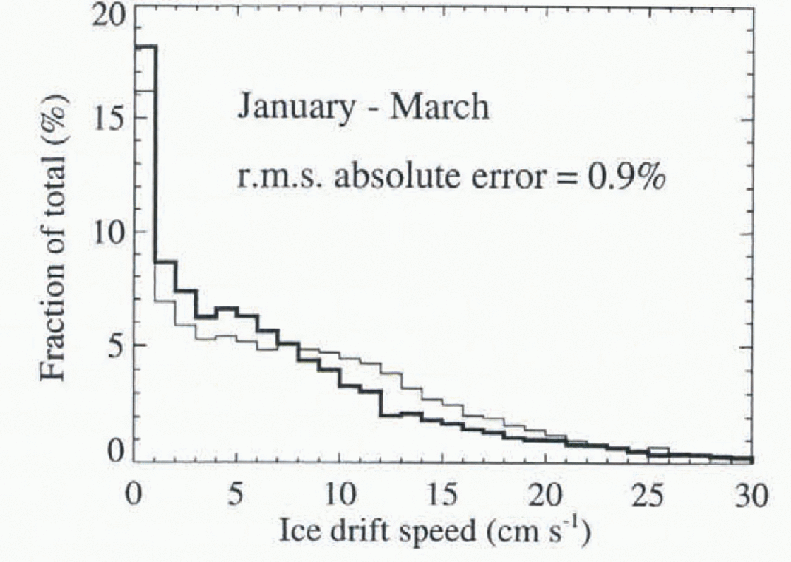
The effects of ice interactions are best reflected in drift-Speed statistics (Reference Lemke, Hibler, Flato, Harder and KreyscherLemke and others, 1997). Speed distributions of the models and the observations are calculated for four seasons (January-March, April-June, July-September, October-December) and five separate regions covering the whole Arctic, each containing about 10 000 daily buoy velocities. The error of the drift characteristics is measured by the root mean square (rms) of speed distribution differences between simulations and observations. An example of rms distribution error is shown in Figure 1 for the viscous-plastic model in the period January-March.

Fig. 1. Observed (thick line) and simulated (thin line) daily speed distributions for buoy data in the period January-March. Error measurement is based on the differences of the individual histogram bars. The root mean square (rms) of these differences is 0.9%.
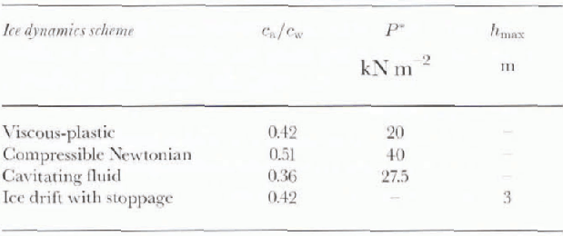
All models are run with different ratios of air and water drag coefficients ca/cw to obtain realistic average daily-drift speed. The ice model with step-function stoppage slows the velocity field so much that it does not make sense to compensate this artificial error with an unrealistically high ratio of drag coefficients. Therefore, the ratio here is set to the value of the viscous-plastic model. Table 1 shows the ratios of drag coefficients used for the different models.
Table 1. Parameter configurations for optimized ice-drift statistics

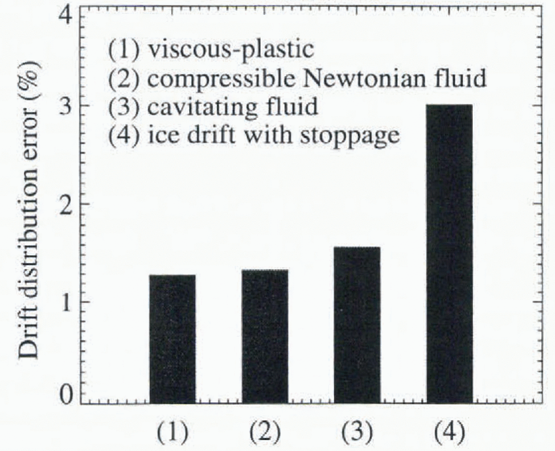
Subsequently, the ice-strength parameter P* (h max for the ice-drift stoppage scheme) is optimized with regard to the rms speed-distribution error. The results (Fig. 2) reflect that the viscous-plastic rheology predicts the most realistic drift statistics, followed by the compressible Newtonian fluid model. The cavitating fluid simulation, with no shear forces, differs significantly because it does not provide ice-drift stoppage near coasts. The ice-drift scheme with step-function stoppage damps the ice drift in an unrealistic way, reflected in the highest error of the drift statistics (Reference Lemke, Hibler, Flato, Harder and KreyscherLemke and others, 1997).

Fig. 2. Rms speed distribution errors (%) for four different dynamic schemes (based on drift-speed statistics calculated for five separate regions and four seasons).
Fram strait ice export
The previous section presented the quality of drift characteristics predicted by the different dynamic schemes. This raises the issue of how important these differences are for the ice export forcing the thermohaline circulation in coupled sea-ice ocean models.
Figure 3a compares the ice thickness at the North Pole for the different models to observations. Seven mean ice-thickness observations at the North Pole from 50 km submarine transects in the period 1986–92 (Reference McLaren, Bourke, Walsh, Weaver, Johannessen, Muench and OverlandMcLaren and others, 1994) are used as verification data. The best prediction of North Pole ice thickness is obtained with the viscous-plastic model. In contrast, the cavitating-fluid model underestimates and the two other schemes overestimate the ice thickness at the North Pole.

Fig. 3. (a) Ice thickness at the North Pole (m), (b) averaged daily-drift speed (cm s−1) in Fram Strait region, and (c) mean ice export through Fram Strait (Sv) for the different models. The horizontal lines indicate the observations.
Figure 3b shows the ice-drift speed in Fram Strait region. The two plastic rheologies slightly underestimate ice-drift speed. The other two models predict drift velocities that are much too low. Ice thickness in the central Arctic and the ice-drift speed in Fram Strait determine the ice export through Fram Strait as displayed in Figure 3c . In agreement with the observed Fram Strait outflow of 0.1–0.16 Sv given by Reference Aagaard and CarmackAagaard and Clarmack (1989), the viscous-plastic and the Cavitating-fluid model both predict a Fram Strait ice export of 0.11 Sv. The other dynamic schemes yield signifi-cantly smaller Fram Strait outflows, and also predict markedly different seasonal cycles of ice export (Fig. 4).

Fig. 4. Time series of mean seasonal cycles of ice export through Fram Strait (Sv) for 1986–92. Results for four different dynamics schemes are shown.
Conclusions
The viscous-plastic model with replacement closure predicts the most reasonable drift statistics and ice thicknesses in the central Arctic. In contrast, the results of the very simple ice-drift scheme with Step-function stoppage clearly show differences in drift characteristics, as well as in ice thicknesses and ice export. The compressible Newtonian fluid simulation shows good conformity with observed drift statistics, but cannot prevent excessive ice-thickness buildup in the central Arctic. Also, the mean seasonal cycle of Fram Strait outflow shows significant differences when compared with the results of the viscous-plastic model. The cavitating-fluid model shows marked differences in drift-speed statistics due to the lack of shear strength. The mean seasonal cycle of ice export is very similar to the viscous-plastic model.
This leads to the conclusion that the plastic behavior of sea ice effectively limits ice-thickness buildup in the central Arctic due to advective processes. A divergent ice flow with little or no internal forces, permitted by the viscous-plastic and the cavitating-fluid models, seems to be a requirement to predict a reasonable Fram Strait ice export. In terms of Fram Strait outflow, the cavitating-fluid model is a good alternative to the more complete viscous-plastic model.
Overall, viscous-plastic rheology yields the most realistic simulation with respect to drift statistics, ice thickness at the North Pole, and Fram Strait outflow.
An overview of SIMIP is given by Reference Lemke, Hibler, Flato, Harder and KreyscherLemke and others (1997) and further, related work is described by Reference HarderHarder (1997).
Acknowledgements
We would like to thank G. M. Flato for pre-processing the IABP buoy-position data, and for providing the results for the cavitating-fluid model. The atmospheric-forcing fields were derived from ECMWF analyses.


