Introduction
The Arctic Ocean and adjacent seas strongly influence the Earth's climate system directly, due largely to the overlying sea-ice cover that creates a high surface reflectance and limits turbulent heat exchanges between the ocean and the overlying atmosphere. Further, the halocline tends to reduce the heat exchange between the surface atmospheric layer and the subsurface oceanic layers in the model. At the same time, high latitude air–sea-ice interaction is the main conduit through which the deep ocean communicates with the rest of the climate system (Reference Mcphee and MartinsonMcPhee and Martinson, 1994).
A key element in understanding oceanic impact on climate is comprehending the processes that control the near-surface exchange of heat, salt and momentum. A modelling approach is well-suited to elucidating these complex interactions. Many authors have found that models exhibit a sensitivity of simulated climate to the treatment of ocean thermodynamics and circulation (Reference Delworth, Manabe and StoufferDelworth and others, 1993), and that the sensitivity of a coupled atmosphere–ocean model is different from that of a simple atmospheric global climate model (GCM).
The relaxing of constraints at the ocean–atmosphere interface introduces new degrees of freedom into the system. Many present-day coupled GCMs exhibit some degree of climate drift, a major concern in studies of climate and climate variability (Reference Stockdale, Latif, Burgers and WolffStockdale and others, 1994). This paper takes a regional-climate modelling approach to the problem of ocean-atmosphere interaction in the Arctic in an effort to understand better the linkages and feedbacks between the atmosphere, ice and ocean without suffering from the biases and simplifications of a global model.
Of fundamental importance is the presence of a surface layer in the Arctic Ocean that extends down to about 200 m (Reference Barry, Serreze, Maslanik and PrellerBarry and others, 1993). While exhibiting various regional characteristics, the surface layer is often “well-mixed” down to about 50 m, with salinities as low as 29 ppt at the surface and increasing with depth. We will discuss the criteria for defining “well-mixed” and how they relate to the model simulations. The presence of this surface layer is determined primarily by continental runoff through mixing from the shelf seas and the Bering Strait inflow. The latter represents almost a third of the total fresh-water input to the Arctic Ocean (Reference Aagaard and CarmackAagaard and Carmack, 1989), and the Bering Strait provides the only avenue of exchange for ice, water and heat between the Pacific and Arctic Oceans. Thus, the western Arctic has been chosen as a focus area for this study.
The Bering Strait is less than 60 m deep and connects two shallow, smooth and extensive shelf regions to the Chukchi Sea to the north and the Bering Sea to the south. The shelf waters are connected to the North Pacific through the Aleutian passes, with water exchange on the order 25–35 Sv. The background flow to the north through the Bering Strait is driven by a mean sea-level slope betweem the Pacific and Arctic Oceans, with an annual mean of 0.8 Sv and a seasonal cycle of amplitude 0.6 Sv, with the maximum in June and the minimum in February (Reference Coachman and AagaardCoachman and Aagaard 1988). The observed strong variability of the Bering Strait flow is primarily caused by the variability in the regional wind field (Reference Aagaard, Roach and SchumacherAagaard and others, 1985), with strong northerly winds reducing the northward transport during the winter.
First, the Arctic Region Climate System Model (ARC-SyM) and the ocean components used in this study of three-month simulations from January to March 1988 will be described. Second the influence of ocean thermodynamics and ocean dynamics are discussed. Finally, the question of the definition of a “well-mixed” layer in an icc-covered ocean is considered.
Model Description
Since the ARCSyM has been described in detail in Reference Lynch, Chapman, Walsh and WellerLynch and others (1995) only a brief Summary will be reproduced here. The atmospheric component is based on the NCAR RegCM2 (Reference Giorgi, Marinucci and BatesGiorgi and others, 1993), a hydrostatic, primitive-equation model with a terrain following vertical coordinates and a staggered “Arakawa B” horizontal grid. The model domain has a horizontal resolution of 63 km and 23 sigma levels in the vertical, with the highest resolution in the boundary layer.
The sea-ice component is based on the cavitating-fluid ice-dynamics scheme of Flato and Hibler (1992) with an anti-diffusion option (Reference Lynch, Glueck, Chapman, Bailey and WalshLynch and others, 1997), and the thermodynamics of Reference Parkinson and WashingtonParkinson and Washington (1979). The thermodynamics formulation is a simple two-layer model allowing for ice, leads and snow cover. The turbulent heat and moisture fluxes are parameterised using the standard bulk aerodynamic formulae, with the turbulent transfer coefficient a function of the near-surface atmospheric stability. The bulk Richardson number is calculated separately over ice and open-water surfaces as a measure of the stability of the near-surface environment (Reference Curry and EbertCurry and Ebert, 1992).
New to this formulation is the addition of mixed-layer and dynamical ocean components. The mixed-layer component is a second-order closure turbulence scheme (Reference Kantha and ClaysonKantha and Clayson, 1994) belonging to the Mellor–Yamada hierarchy, but with some modifications (Reference Galperin, Kantha, Hassid and RosatiGalperin and others, 1988). The surface boundary of the water column is forced by the sensible and latent heat fluxes, the radiative fluxes, the precipitation–evaporation rate (at open ocean and lead areas), melting–freezing rates (ice-covered areas), and surface stresses at the ice–ocean or atmosphere–ocean interfaces. The one-dimensional (1-D) mixed-layer formulation then solves the turbulence-closure equations for the temperature, salinity, mean velocity components, turbulent energy, and mixed-layer depth. The model is configured with one water column at open-ocean gridcells, and two water columns at ice-covered gridcells. The latter allows for the calculation of separate lead-to-atmosphere and ice-to-atmosphere fluxes. The amount of the shortwave radiation that reaches the ocean through the ice and snow cover is decreased exponentially with ice and snow thickness. This is a generalised curve based on the findings of Reference Ebert, Schramm and CurryEbert and others (1995), who considered the extinction of several shortwave bands in different types of ice cover. The incoming longwave is generally assumed to be absorbed in either the snow layer or very thin upper ice layer.
The dynamical ocean model is the S-coordinate primitive-equation ocean-circulation model SPEM Version 5.1, which has a rigid lid approximation and a generalized topography following the S-coordinate in the vertical (Reference Haidvogel, Wilkin and YoungHaidvogel and others, 1991; Reference Aagaard, Roach and SchumacherSong and Haidvogel, 1994). This coordinate is capable of simultaneously maintaining high resolution in the surface layer as well as dealing with steep and deep bathymetry.
The model domain is a region of the western Arctic centred on the Bering Strait. The bathymetry for this region, smoothed from the ETOPO5 global ocean-topographv data-set, is shown in Figure 1a, and the orography is shown in Figure 1b. The ocean model boundary conditions for this domain are specified as follows: a barotropic inflow of 10.8 Sv into the Gulf of Alaska is fixed, balanced by a barotropic outflow of 10 Sv on the western side of the Bering Sea, and 0.8 Sv northward through the Bering Strait and into the Arctic Ocean. The surface-water salinity is set to 30 ppt and the sea ice is assumed to be fresh. The atmospheric boundary conditions are provided by 12 hour European Centre for Medium-Range Weather Forecasts (ECMWF) analyses as described in Reference Lynch, Chapman, Walsh and WellerLynch and others (1995). Three model experiments were performed on this domain as follows:
-
(1) Coupled atmosphere–ice simulation: the model was initialized on 1 January 1988 using ECM WF analyses, and a uniform ice cover 2 m thick with 99.5% concentration. Ice concentration and thickness spin-up relatively quickly from these arbitrary initial conditions. Initial ice-edge data were obtained from the weekly ice charts of the Navy-NOAA Joint Ice Center; snow cover over land was initialized to 0.3 m depth at all grid points that were initially colder than 0 C (all land points during this season). The slab ocean temperatures were initialised from the data of Reference Shea, Trenberth and ReynoldsShea and others (1992), with modifications for compatibility with observed ice cover. The deep-ocean heat flux was fixed at 2 W m−2 upwards as described in Reference Parkinson and WashingtonParkinson and Washington (1979).
-
(2) Coupled atmosphere–ice–mixed-layer-ocean model: the atmosphere and ice components were initialised as in experiment A. The water column down to 50 m below the surface was modelled at 1 m vertical resolution for this simulation and initialised with a uniform temperature from the Shea SST. Salinities were initialised at 30 ppt in ice-covered areas, and 33 ppt in open-ocean areas. The mean velocity components were started at rest and forced by the ice–water or air–water stresses.
-
(3) Coupled ice ocean simulation: the sca-ice conditions were initialised as in experiment A. The ocean, containing 16 vertical S-coordinate levels, was initialized in the ice-covered gridcells with zero currents and an averaged profile based on the Levitus ocean atlas (Reference Levitus and GelfieldLevitus and Gelfield, 1992) for salinity and temperature, typical for the Arctic Basin. The open-ocean gridcells were initialised with the Shea SST and a uniform salinity of 33 ppt down to a depth of 50 m, and an averaged Levitus profile typical of the North Pacific Ocean below 50 m. Surface winds, radiative fluxes. specific humidity and surface-air temperature from experiment A were used as forcing for the ice–ocean model.
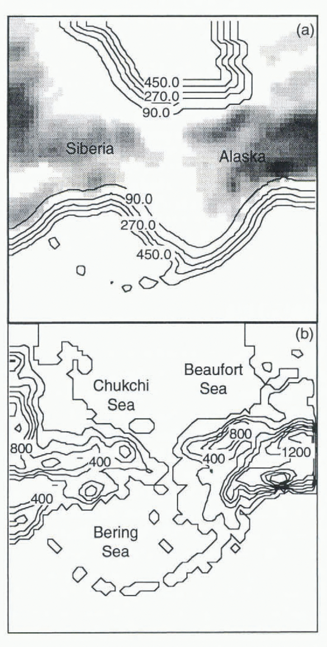
Fig. 1. Computational domain showing (a) bathymetry (m) and (b) orography (m). Note that maximum ocean depth is limited to 550 m.
Influence of Ocean Thermodynamics
Experiment A provides an adequate base state of ice concentrations in the high Arctic when compared to the GISST2.2 dataset (Reference Parker, Jackson and HortonParker and others, 1995). Figure 2 shows the monthly mean ice concentrations for March — note the low resolution of the GISST2.2 data (1) compared to the regional model. However, experiment A shows ice growing thermodynamically in the southern Bering Sea region in February and March, where it does not typically appear. This is due to cold simulated atmospheric temperatures (not shown), which act to cause ice growth without the ameliorating effect of oceanic feedbacks. In experiment B, with the mixed-layer ocean, the overall ice distribution is much thinner due to the warmth of the underlying ocean. As a result, the simulated ice edge (Fig. 3) is more realistic than in experiment A, yet a comparison with the GISST2.2 data-set shows the temperatures in the mixed-layer case to be overestimated by up to 5 in the most southern parts of the domain. The surface flux formulation in the coupled model is currently very simple, and these results suggest that a more sophisticated formulatiou max be necessary. Further, an absence of ocean dynamics allows a positive feedback between surface fluxes, air and ocean temperatures, which is not mitigated by lateral transport.
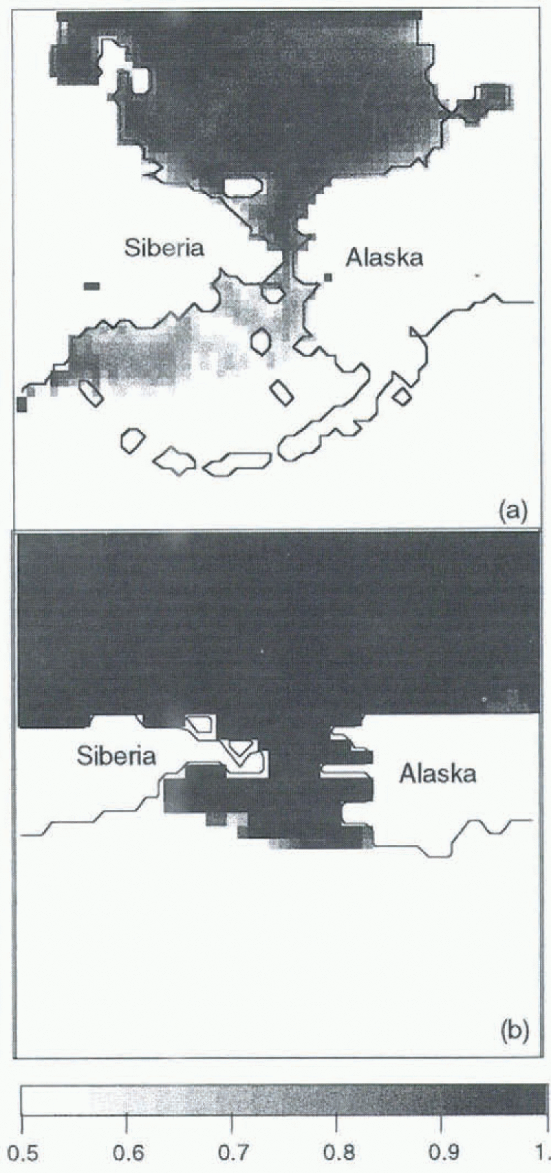
Fig. 2. Monthly mean ice concentration for March, for (a) experiment A and (b) GISST2.2 data.
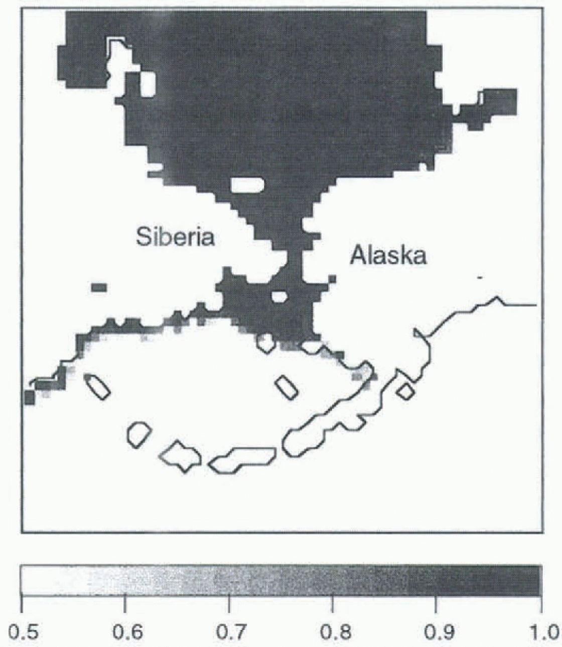
Fig. 3. Monthly mean ice concentration for March, for experiment B with the mixed-layer model.
Influence of Ocean Dynamics
Experiment C is driven by the output of experiment A, which includes the cold-air temperatures in the southern Bering Sea. Despite this, the addition of a three-dimensional (3-D) ocean model, which includes a predictive ocean temperature, produces a more realistic ice concentration in the southern Bering Sea (Fig. 4). The positive feedbacks leading to the excessive ice in experiment A and the excessive ocean temperatures in experiment B, are absent in this case. The interaction of ocean dynamics and thermodynamics with the ice is still present, and indicates a reduction of ice growth, but not at the expense of excessive ocean temperatures. The ice edge in this case still extends too far south, and concentrations are generally low. It is expected that an implementation of a fully coupled model that includes ocean dynamics and a mixed-layer formulation will reduce the unrealistic ice growth in the Bering Sea and improve the overall sea-ice distribution. Prior to this implementation, it is necessary to consider the appropriate definition for the mixed layer in ice-covered oceans.
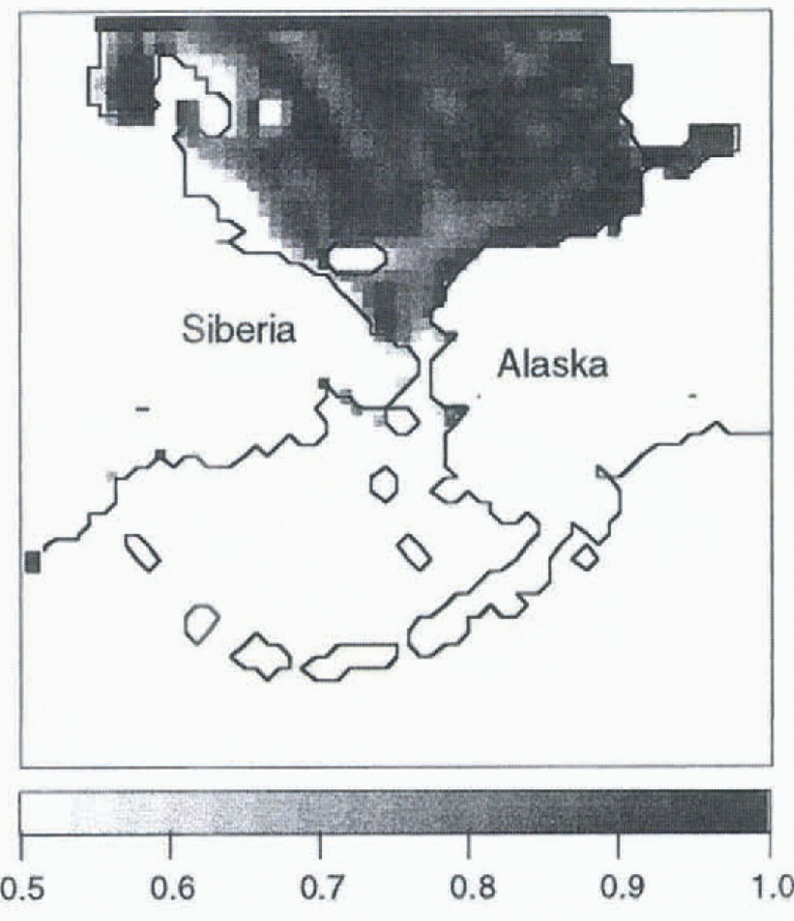
Fig. 4. Monthly mean ice concentration for March, for experiment C with the 3-D ocean model.
Definition of the “Mixed Layer”
The Reference Parkinson and WashingtonParkinson and Washington (1979) ice-thermodynamics scheme assumes that the increase in the fraction of ice in a gridcell is tied to the energy balance of a constant depth and uniform temperature ocean mixed layer. Reference Barry, Serreze, Maslanik and PrellerBarry and others (1993) also consider a temperature-dependent criterion, in which the mixed-layer depth is defined by some maximum difference (generally 0.2–1.0 K) between surface temperature and the temperature at that depth. It is also possible to employ a similar criterion based on salinity. Reference Kantha and ClaysonKantha and Clayson (1994) and Reference Large, Williams and DoneyLarge and others (1994) consider a criterion based on turbulence, which assumes the base of the ocean mixed layer occurs at a depth where the turbulence parameter drops below a certain threshold. While this criterion is consistent with the atmospheric analogy of the boundary layer, it remains that the ice-fraction growth assumption of Reference Parkinson and WashingtonParkinson and Washington (1979) is based on a uniform-temperature mixed layer, which would imply the temperature criterion is more applicable to this use. In addition, the presence of ice at the surface can have a strong impact on the sturcture of the mixed layer.
In an attempt to understand better the impact of these criteria, 1-D experiments were performed with a 200 m water column using the Reference Kantha and ClaysonKantha and Clayson (1994) mixed-layer ocean model. The surface forcing for the three months from experiment A was used in two situations: (i) at an open-ocean gridcell in the southern part of the domain, and a gridcell in the high Arctic for both the (ii) ice-covered and lead areas of the cell. In these experiments a temperature difference of 0.2 K, a salinity difference of 0.1 ppt, and a turbulence parameter threshold value of 1.0 × 10⁻⁹ were used as the three criteria.
It was found that for open ocean and leads, the entire water column became well-mixed very quickly, by all criteria. Various initial conditions were tested, from stably stratified to well-mixed, and this behaviour was found to be independent of the initial conditions. From January to mid-March the solar radiation is negligible because of the reduced daylight hours. Thus, very strong upward surface fluxes (Fig. 5b) lead to rapid cooling of the surface layer, and subsequent overturning of the water column.
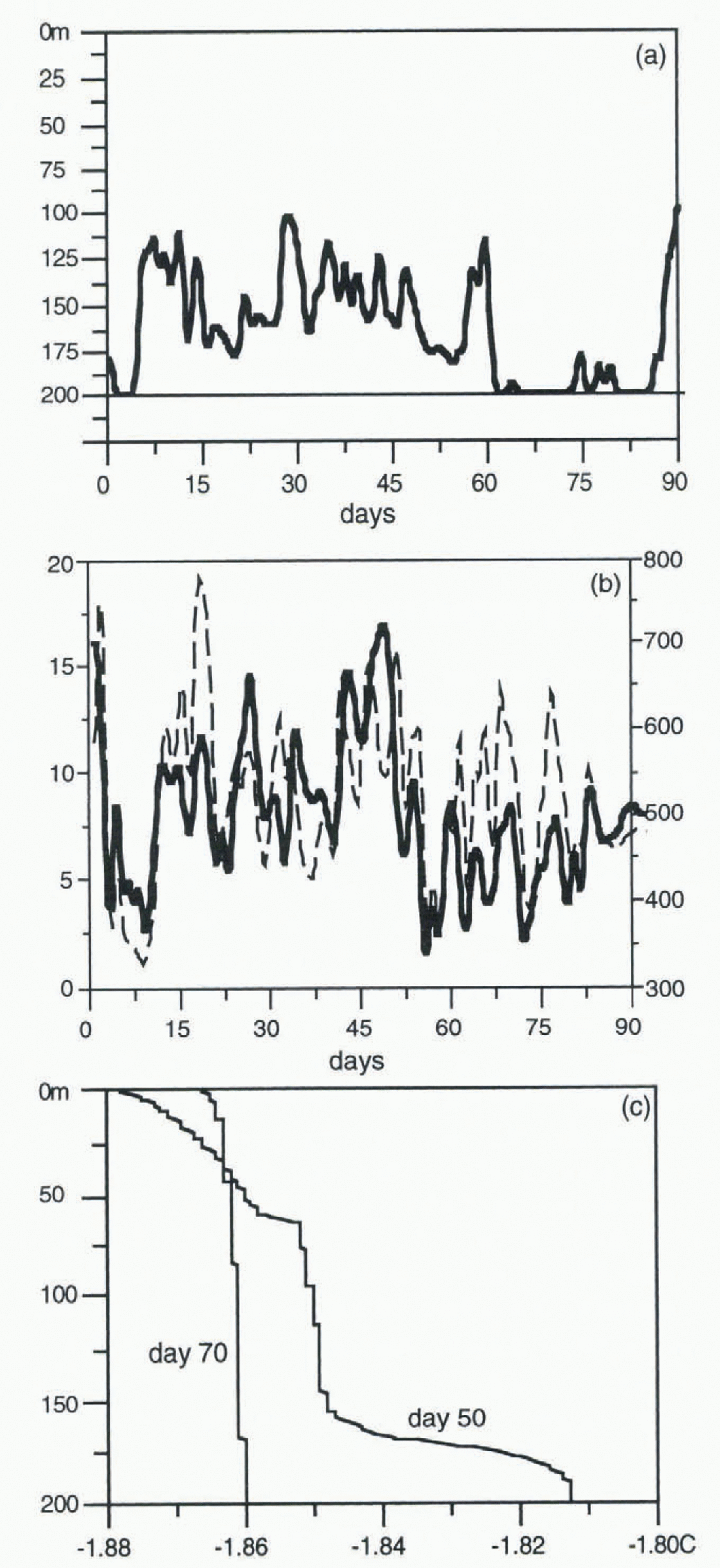
Fig. 5. (a) Mixed-layer depth (m) by the turbulence criterion (bold line) and the temperature and salinity criteria (narrow line at 200 m). Ocean surface is at 0 m. (b)Net fluxes at the surface for the water column under the ice (bold, left axis) and that under the lead (dashed line, right axis) in W m2 (c) Temperature profiles for the water column under the ice at day 50 and day 70 of the integration. Ocean surface is at 0 m.
Under ice-covered areas, the situation was very different. In addition lo negligible solar radiation, precipitation and evaporation do not affect the ocean in these areas. The main surface forces in the ice-covered areas include the flux of heat due to ice thermoconductivity, ice freezing and melting (including runoff from surface melt), and ice-drag. However, while the salinity and temperature-dependent criteria indicated that the entire water column was well-mixed, the turbulent criterion did not. Figure 5a shows the predicted mixed-layer depth for the 3 month integration under the ice. The turbulence criterion shows that the entire water column does not remain turbulent for the whole period. As the surface fluxes of heat (Fig. 5b), salinity and ice-drag are relatively small, the deep-ocean heat flux allows the deeper water to become stably stratified over time. Figure 5c shows the temperature profile for day 50 (which is well-mixed to 160 m by the turbulence criterion) and day 70 (which is well-mixed throughout the entire water column by all criteria). The temperature profile at day 50 indicates that there is stratification below 160 m, yet the temperature criterion is not strict enough to reflect this.
Summary and Discussion
The experiments in this paper have shown that a mixed-layer formulation has improved the overall ice distribution in the western Arctic region, but at the expense of producing sea-surface temperatures that were too warm. This is partially due to the simplicity of the assumptions in coupling the mixed-layer ocean to the ice thermodynamics, and also in the simplicity of the ice thermodynamics itself. The use of an ice model coupled to a 3-D ocean model without a mixed-layer formulation can also improve the ice distribution without the warmer sea-surface temperatures, and could be coupled to the atmospheric model in future runs. Moving to a simulation using a coupled atmosphere–ice–ocean model that includes the 3-D dynamical ocean primitive equations together with a mixed-layer formulation is expected to combine the best aspects of the two experiments. However, there is a need to choose proper criteria for calculating the mixed-layer depth under the ice. It appears that a turbulence-based formulation is the most accepted and more representative of the changes in the mixed laver under the Arctic ice cover. The present ice-model thermodynamics could be adapted to include this, or a new ice-thermodynamic formulation could be incorporated.


