Lidar-Derived Particle Concentrations in Plumes from Arctic Leads

Abstract

With an airborne lidar, we have observed massive plumes of condensate particles rising from wintertime leads in the Arctic Ocean. Some of these plumes reached an altitude of 4 km; some extended over 200 km down-wind from their surface source. Here we invert the lidar equation and use lidar backscatter data to infer particle concentrations within two such plumes. Assuming that the plumes consist of supercooled water droplets of radius 5 μm, we estimate typical concentrations of 3–6 × 10⁵ droplets m^-3 just above the leads. Concentrations within the plumes can still be as high as 10⁴ droplets m^-3 at an altitude of 3 km and 200 km down-wind from some leads. Had we assumed that the plume particles are ice spheres of radius 40 μm, concentrations would be just 100 times less than these.

Plumes From Leads

Leads and polynyas are regions of open water or thin, newly formed ice that occur in the pack ice of the Arctic Ocean in response to wind and currents. They are climatologically important because in winter heat passes through leads from the relatively warm ocean to the cold atmosphere two orders of magnitude faster than it does through the ubiquitous ice (Badgley, 1966; Maykut, 1978; Andreas and others, 1979).

Several experiments over narrow leads and polynyas (Badgley, 1966; Andreas and others, 1979, 1981; Smith and others, 1983) did not dispel the notion that the heat and moisture lost from open water in winter remains within the atmospheric boundary layer, trapped by the prevalent Arctic inversion. But we have recently documented high-rising plumes of water droplets or ice crystals that clearly originated from major leads north of Ellesmere Island (Schnell and others, 1989). Some of these plumes reached an altitude of 4 km, while others extended down-wind from their surface source over 200 km. They were massive. Such leads and their associated plumes may produce basin-wide climatological effects.

To continue toward our ultimate goal of understanding how much lead-derived heat and moisture reaches an arbitrary level in the atmosphere, we here estimate particle concentrations in two of these massive plumes. The plumes were observed with an airborne, downward-looking, 1.06 μm lidar; we convert the Rayleigh (backscatter) ratio measured by the lidar into plots of particle concentrations within the plumes.

The Lidar Equation

A lidar experiencing backscattering obeys (Collis and Russell, 1976)

(1)

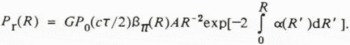
Here, P_r is the instantaneous received power; Ρ₀ , the transmitted power; R, the range to the scatterer; G, a calibration constant; c, the speed of light; τ, the lidar pulse duration; R′, position along the propagation path; β_π and α, respectively, the volume backscattering coefficient and the volume extinction coefficient of the atmosphere; and A, the receiver area.

The extinction α results from two effects, molecular scattering and absorption (α_a) and aerosol scattering and absorption (α_a) (Collis and Russell, 1976); thus

(2)

The backscattering coefficient, likewise, is the sum of molecular (β _πm) and aerosol (β _πa) backscattering,

(3)

From the lidar observations, we computed the so-called Rayleigh ratio B, the ratio backscattered power from an aerosol cloud to backscattered power from clear air, where this clear-air backscatter value came from flight segments through clear air. From Equations (1)–(3), the Rayleigh ratio is

(4)

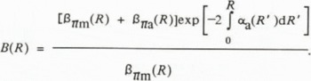
Because the aerosol backscattering coefficient depends on the number of aerosol particles present through

(5)

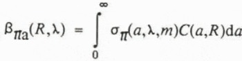
where λ is the lidar wavelength, σ_π is the backscattering cross-section, and C is the number concentration of particles with radius a and complex refractive index m, we have a means of estimating particle concentrations from the Rayleigh ratio.

A few simplifying assumptions are, however, necessary. Andreas and others (1981) concluded that the vapour escaping from wintertime leads condensed into droplets having a fairly narrow size distribution with a mode radius of about 5 μm. Such small droplets can persist supercooled even at Arctic temperatures (Schaefer, 1962; Andreas and others, 1981; Heymsfield and Sabin, 1989). Sampling at higher altitudes, Ohtake and others (1982) found that the particles over Arctic leads were ice crystals with a mode radius more like 40 μm But because they were unable to sample particles with radii smaller than 10 μm, 40 μm is probably an upper limit for the mode radius of these crystals. For our calculations, we henceforth assume that a lead plume is a mono-dispersive aerosol consisting either of supercooled, spherical water droplets of radius 5 μm, or spherical ice crystals of radius 40 μm.

The backscattering cross-section in Equation (5) is usually expressed in terms of a dimensionless back-scattering efficiency factor Q _π (x,m),

(6)

where x = 2πa/λ is a size parameter. Because we assume that the plume consists of particles of a single size, Equation (5) thus becomes

(7)

We computed Q_π using the Mie theory computer program given by Bohren and Huffman (1983: 477–82), with values for the refractive index of water (Irvine and Pollack, 1968) and of ice (Warren, 1984) at 1.06 μm. For 5 μm water droplets, x = 30 and Q_π = 0.23; for 40 μm ice spheres, x = 240 and Q_π = 0.36.

The aerosol extinction coefficient, α_a, in Equation (4) is also related to a cross-section, the extinction cross-section σ_ex(a,λ,m), as in Equation (5). and this cross-section, in turn, is usually expressed in terms of the extinction efficiency factor Q_ex(x,m), in analogy with Equation (6). Thus, for a monodispersive aerosol, α_a can be modeled as β _πa in Equation (7), α_a(R,λ) = πa²Q_ex(x,m)C(a,R), where from our Mie calculations Q_ex ≃ 2. From McClatchey and others (1972), we estimate that α_a is in the range 6 × 10⁻⁵ to 2.6 × 10 m⁻¹; from Collis and Russell (1976), 1–5 × 10 ⁻⁴ m⁻¹. For the droplet concentrations that Andreas and others (1981) measured over leads, we estimate that dg is roughly 1.9 × 10⁻⁴ m⁻¹; from the conditions observed by Ohtake and others (1982), we estimate 2.0 × 10 ⁻⁴ m⁻¹. Because of the limited range in these estimates, for our subsequent calculations we assume that α_a= 2.0 × 10⁻⁴ m⁻¹.

Finally, we can compute the molecular backscattering coefficient, β _πm, in Equation (4) from a relation given by Penndorf (1957) and McCartney (1976),

(8)

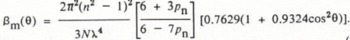
Here β_m(θ) is the molecular scattering coefficient at angle θ, Ν is the number density of air molecules, and p_n (= 0.035) is the depolarization factor. For backscatter, θ = 180°; thus, β _πm ≡ β_m(180 °). Ν derives simply from N = ρN _a/M _a where ρ is the air density, N_a is Avogadro’s number, and M_a is the molecular weight of air. For n, the real part of the refractive index of air, we use Owens’ (1967) relation.

With Equation (7), with the relation for molecular backscatter [Inline 16] (Equation (8)), and with the other simplifications that we have been discussing, we can derive from Equation (4) a prediction equation for the particle concentration within lead plumes,

(9)

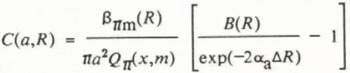
where ΔR is the range increment for which the lidar beam was within the plume.

Because the B(R) term within the square brackets in Equation (9) is generally much larger than 1, C is almost directly proportional to Β and inversely proportional to exp(α_a), to exp(ΔR), and to Q_π. Our Mie computations showed that Q_π is very sensitive to particle size; uncertainty in the particle radius, therefore, probably introduces a factor-of-five uncertainty in our concentration estimates through the a² and Q_π terms in Equation (9).

Particle Concentrations in the Plumes

We here consider the lidar data collected on 27 January 1984 during the Arctic Gas and Aerosol Sampling Program (AGASP) (Schnell, 1984). Figure 1 shows the flight track north from Thule, over Alert, and then out over the frozen Arctic Ocean (Kent and others, 1986). Nominal flight altitude was 5800 m. In the figure we also show major leads visible in Defense Meteorological Satellite Program (DMSP) infrared images from the time of the flight. At least two of these leads, as marked in the figure, were open and produced major plumes that we have documented elsewhere (Schnell and others, 1989). We derive particle concentrations in these two plumes.

Fig. 1. Flight track out of Thule, Greenland, on 27 January 1984. Major leads along the flight track that are visible in DMSP images are indicated. The two plumes discussed in this paper originated in the leads marked 1 (Fig. 2) and 2 (Fig. 3) in the figure.

The flaw lead north of Ellesmere Island produced an enormous plume that reached an altitude of 3 km and extended down-wind (northward) over 200 km (Fig. 2). Although we do not have information on the width of this lead, the surface droplet concentrations in Figure 2 and near-concurrent satellite imagery suggest that it may have been at least 20 km wide.

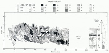
Fig. 2. Concentrations of 5 μm water droplets computed for the plume observed between 16.35 and 17.05 Ζ that originated in the flaw lead north of Ellesmere Island. If the plume particles were 40 μm ice spheres, instead of water droplets, concentrations would be just 100 times less. The origin of the abscissa is arbitrarily located.

The second plume (Fig. 3) originated in a lead at about 85°N, well into the interior of the Arctic ice pack. This plume reached an altitude of almost 4 km. Although again we have no direct observations of the width of this lead, given the meteorological conditions measured by the 12.00 Ζ Alert radiosounding on 27 January, we estimated that a lead would have to be roughly 10 km wide to provide the thermal energy necessary for a plume to reach 4 km (Schnell and others, 1989). Satellite imagery and the maximum in calculated surface droplet concentration shown in Figure 3 corroborate that the lead was roughly 10 km wide.

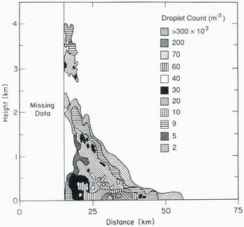
Fig. 3. As in Figure 2, except this is the plume observed between 16.25 and 16.30 Z.

Figures 2 and 3 show the concentrations of droplets with radius 5 μm. For ice crystals with radius 40 μm, the concentrations are just 100 times less. The figures generally give droplet concentrations to only one significant figure to indicate the uncertainty in our calculations. In taking α_a to be a constant of 2 × 10⁻⁴ m⁻¹, in effect, we are assuming that plumes of 5 μm droplets have a uniform concentration of 130 × 10⁴ droplets m⁻³ or plumes of 40 μm ice spheres have a concentration of 2 × 10⁴ crystals m⁻³. Consequently, Equation (9) overestimates the particle concentration in regions for which the overlying plume has concentrations greater than 130 × 10⁴ droplets m³ (or 2 × 10⁴ crystals m⁻³), which is everywhere within both plumes. Therefore, considering the uncertainties discussed earlier, we feel that the concentrations in Figures 2 and 3 are accurate to within an order of magnitude.

The 5 μm droplet concentrations are somewhat smaller than those observed by Andreas and others (1981) within a meter of the surface of narrow leads. They found maximum condensate concentrations of 1–20 × 10⁷ droplets m⁻³. But because the lidar has a vertical resolution of about 30 m, it cannot measure as near the surface as Andreas and others did; as a result, it yields maximum concentrations somewhat less than they found.

Except in the immediate vicinity of their source, these plumes have particle concentrations lower than those measured in most clouds (Carrier and others, 1967). The bulk of a plume is therefore not visible. In fact, plume particle concentrations are typical of subvisible cirrus clouds (Braham and Spyers-Duran, 1967; Hoff, 1988; Sassen and others, 1989). In light of the computed concentrations, knowing that the ambient air temperature was near −30°C in the lower 4 km, and realizing that the relative humidity needs to be only about 75% for air to be saturated with respect to ice at −30°C, we conclude that the bulk of the observed plumes consist of ice crystals.

The 12.00 Ζ Alert radiosounding on 27 January showed a main inversion at 600–700 m and an overall drop in potential temperature of 25°C between the surface and 1500 m. Yet such atmospheric stability was clearly unable to constrain the plumes near the surface. With lead-derived heat and moisture, thus, capable of reaching the mid-troposphere, wide leads have the potential to influence the climate not just locally but basin-wide.

Though invisible, the plumes may also affect the climate radiatively. Assuming ice crystal concentrations of 1–100 × 10⁴ m⁻³, Curry and others (1989) computed infrared radiative cooling rates in- the Arctic atmosphere that were about 2°C d⁻¹ greater than for clear air. This atmospheric radiation loss would, in turn, warm the sea-ice surface and have significant influence on the surface energy budget. The plumes shown in Figures 2 and 3 both have particle concentrations similar to those used in the calculations by Curry and others. Thus, the Ellesmere Island flaw lead (Fig. 2) has, in effect, thrown a warming blanket of condensate particles over the sea ice for more than 200 km down-wind. Similar leads that occur in the marginal seas north of Siberia probably produce like effects in that area.

Acknowledgements

We would like to thank G. Koh, J.A. Curry, K.C. Jezek, S.G. Warren, and an anonymous reviewer for comments on the manuscript. Discussions with A.W. Hogan were very helpful. L.F. Radke, C.A. Brock, M.P. McCormick, and J.L. Moore provided technical help with the data collection and processing. The U.S. Office of Naval Research supported this work with contracts N0001486K0695, N0001488WM22012, and N0001489WM22006.