1. Introduction
The dynamics of calving glaciers are poorly understood. A number of observational and modeling studies have been done that focus on the details of the calving process and the response of the glacier snout (e.g. Reference Funk and RöthlisbergerFunk and Röthlisberger, 1989; Reference HughesHughes, 1992; Reference Van der VeenVan der Veen, 1996; Reference Kirkbride and WarrenKirkbride and Warren, 1997; Reference Fischer and PowellFischer and Powell, 1998). In these studies, the discussion focuses on the importance of local mechanics and interaction with the bed, as opposed to the role of glacier sliding and hydraulics. There is no consensus about the factors that dominate the evolution of tidewater glaciers. Reference Van der VeenVan der Veen (1996) argues that processes acting at the glacier bed are most important.
In the following we restrict the discussion to tidewater glaciers, i.e. calving glaciers that are not floating. It has been stated many times that tidewater glaciers are inherently unstable and are able to exhibit self-sustained oscillations which are not or only weakly coupled to climate change (e.g. Reference ClarkeClarke, 1987; Reference Meier and PostMeier and Post, 1987; Reference WarrenWarren, 1992). Nevertheless, on longer timescales it must be the climatic conditions that determine the fate of any glacier. It cannot be ignored that during the last century the number of retreating tidewater glaciers has been significantly larger than the number of advancing tidewater glaciers. This can only be attributed to glacier thinning associated with less favourable climatic conditions, notably higher temperatures.
Very few modelling studies have been published in which the global (qualitative) dynamics of tidewater glaciers are considered and a full cycle of retreat and advance is simulated. Perhaps the most comprehensive study is that by Reference Vieli, Funk and BlatterVieli and others (2001). Vieli and others combine a fairly sophisticated two-dimensional (vertical plane) numerical ice-flow model with the modified flotation criterion suggested by Reference Van der VeenVan der Veen (1996). The model simulates well rapid retreat and slow advance of the glacier terminus across overdeepenings in the bed. Reference Vieli, Funk and BlatterVieli and others (2001) also argue that a linear relation between water depth and calving rate may hold for relatively slow changes, but not for very rapid retreat.
Although the study of Reference Vieli, Funk and BlatterVieli and others (2001) shows very interesting results, a few questions remain. First, it is not clear if the detailed treatment of the ice flow is needed to generate the typical behaviour of fast retreat/slow advance. In fact, one may argue that any model in which the calving rate is somehow related to water depth will produce this characteristic. Secondly, Reference Vieli, Funk and BlatterVieli and others (2001) did not carry out a systematic study of the equilibrium states of their model, but focused on a few transient scenarios. It would be interesting to know if for a bed profile with overdeepenings every terminus position could represent a steady state, or that there is branching of the equilibrium solutions and hysteresis.
In this paper, we take a different approach and want to find a simple model that exhibits the same dynamical behaviour as the model of Reference Vieli, Funk and BlatterVieli and others (2001). Moreover, we want to construct a model that mimics the full cycle of ice-free conditions, glacier terminus on land, calving glaciers terminus, and backwards. We do not deal explicitly with ice mechanics but focus on the role of the bed geometry. The model glacier has a steep front, also when it ends on land. The ice thickness at the glacier front is parameterized in terms of glacier length and, when the glacier is calving, water depth. We use a linear relation between calving rate and water depth (Reference Brown, Meier and PostBrown and others, 1982; Reference Pelto and WarrenPelto and Warren, 1991; Reference Björnsson, Pálsson and GudmundssonBjörnsson and others, 2000). We acknowledge that such a relation is not generally applicable (Reference Van der VeenVan der Veen, 1996), but it certainly provides a first-order estimate of mass loss at the calving front.
The calving rate and the surface mass balance averaged over the glacier make up the total mass change. In our model, the change in glacier length is determined by the total change in the mass budget and the shape of the bed, but not by the details of the glacier profile and the related velocity field. We will show that this may still yield relatively rapid rates of retreat. We regard the present model first of all as a learning tool, which reveals that even for a simple mathematical representation of a glacier the dynamics become strongly non-linear due to height-mass-balance feedback and the water-depth-calving-rate feedback.
In this paper, we describe the model and investigate its properties for an idealized bed geometry with a smooth overdeepening. We study two cases: (i) a glacier with a specific balance (accumulation) that is spatially uniform, and (ii) a glacier in a warmer climate with the specific balance a linear function of altitude. In case (i) the role of the bed topography appears in a pure form. In case (ii) the dynamics are richer, because a changing mean glacier thickness affects the surface mass balance.
2. Model
The geometry of the model is shown in Figure 1. The surface profile of the glacier has been drawn in a rather arbitrary way, because the details of the profile do not enter into the mathematical formulation of the model. The head of the glacier is at x = 0, and here the horizontal flux of ice is zero (so this point could also be regarded as the dome of an ice cap). One of the basic assumptions is that the mean ice thickness (Hm) and the ice thickness at the glacier front (Hf) can be related in a simple way to the glacier length (L). The expressions used are:
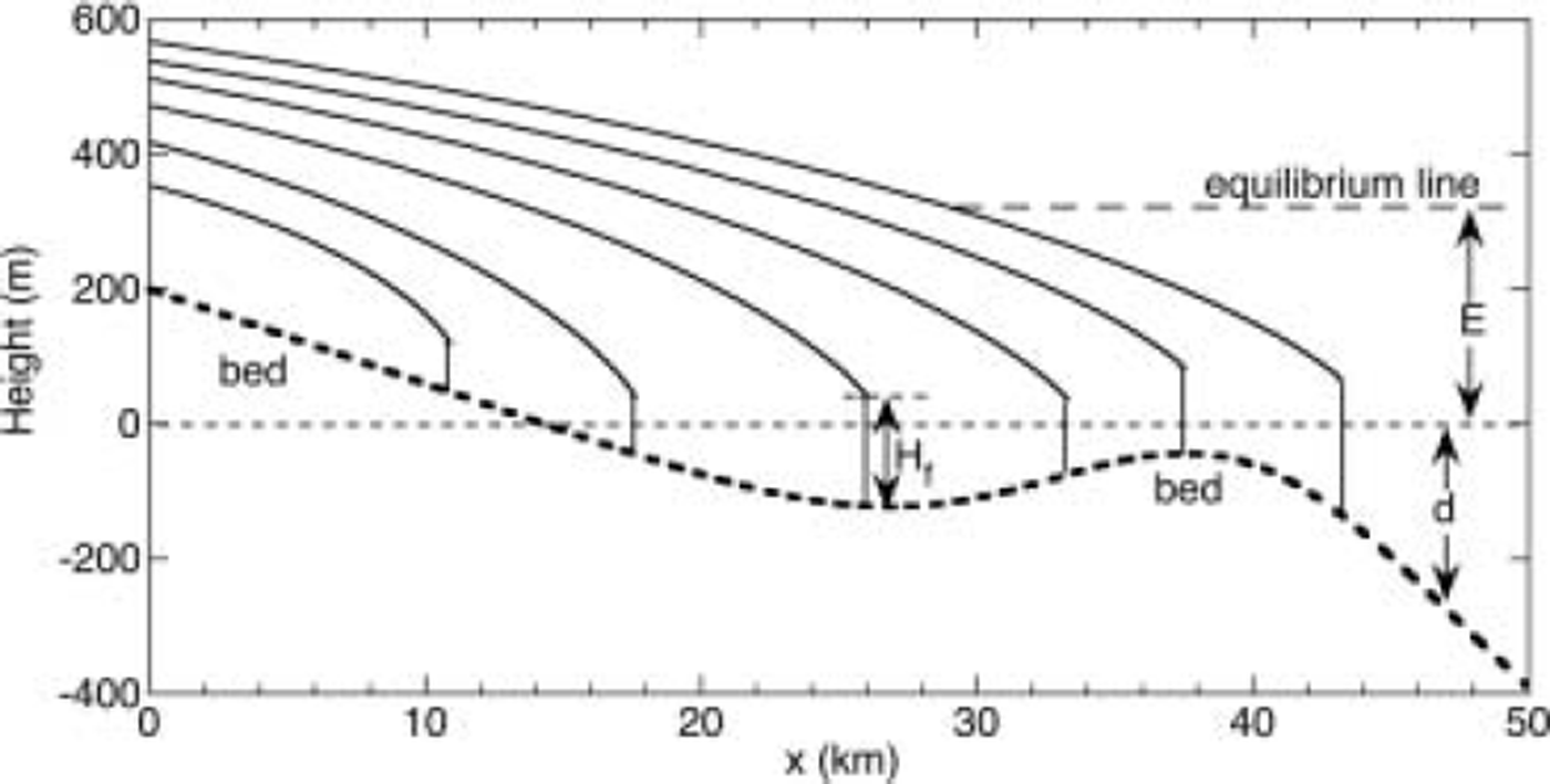
Fig. 1. Geometry of the glacier model. H f is the ice thickness at the front, d(x) the bed elevation with respect to sea level, and E the altitude of the equilibrium line. The surface profiles have been drawn arbitrarily. In the model, the geometry of the glacier is characterized only by glacier length, ice thickness at the front, and mean ice thickness.
In these equations, am and af are constants that are related to the bulk flow parameter of the glacier (involving deformation and sliding). The square-root dependence of ice thickness on L is inspired by the theory of ice-sheet flow (Reference VialovVialov, 1958; Reference WeertmanWeertman, 1961) and extensive calculations with a numerical glacier model (Reference OerlemansOerlemans, 2001, p. 69). In Equation (2), d is the bed elevation with respect to sea level, and δ the ratio of water density to ice density. So d is negative when the bed is below sea level, and -δd is the ice thickness at which the ice just starts to float. A parameter ε is included to specify to what extent the frontal thickness is above buoyancy. Altogether, Equation (2) states that the ice thickness at the glacier front is determined by the water depth, unless this thickness drops below the frontal thickness in case of a land-based glacier. This formulation allows a smooth transition from a glacier with the terminus on land to a tidewater glacier. It also implies that the height above buoyancy at the glacier front may increase when the glacier advances across a sufficiently shallow sill (see Fig. 1).
Adapting a linear relation between calving speed and water depth (with constant of proportionality c) now yields, for the flux of ice at the glacier front:
Note that F is a negative quantity because it represents loss of mass.
We use two different formulations for the surface mass balance. In the first case, the mass balance is constant and equal to the accumulation rate a. Therefore the total gain of ice at the surface simply is
In the second case, we assume that the balance is a linear function of altitude with respect to the equilibrium-line altitude E. Then we have
Here β is the balance gradient (with respect to altitude), and hm the mean altitude of the glacier surface. Later we will discuss how hm is estimated.
The evolution of the glacier is calculated from the conservation of mass:
Since we want to calculate the change in glacier length, dL/dt has to be related to dV/dt. It is easily verified that:
From Equations (6) and (7) it follows that
Equation (8) cannot be solved analytically, unless the glacier terminates on land and the bed profile is linear (in that case, the resulting equation for glacier length is quadratic; Reference OerlemansOerlemans, 2001). However, it is very simple to integrate Equation (8) numerically.
The following bed profile is adopted for the calculations:
This represents a bed sloping linearly downwards (s>0) on which a Gaussian-shaped bump of amplitude λ and width a is superimposed (Fig. 1). The location of the bump is determined by x s. Overdeepening of the bed occurs for a sufficiently large value of A.
3. The Case of a Uniform Mass Balance
We first consider the case in which the mass balance is independent of x. The accumulation rate a is increased at a rate of 0.0005 m ice a-1 (Fig. 2a). Such a change in a should be sufficiently slow to let the model glacier be in quasi-equilibrium most of the time. The bed parameter values are d 0 = 200 m, s = 0.014, λ = 300 m, xs = 40 km and σ = 10km. The corresponding profile is shown in Figure 1. So we are actually looking at a large valley glacier in cold conditions, flowing into a shallow sea with an overdeepening of a moderate amplitude.
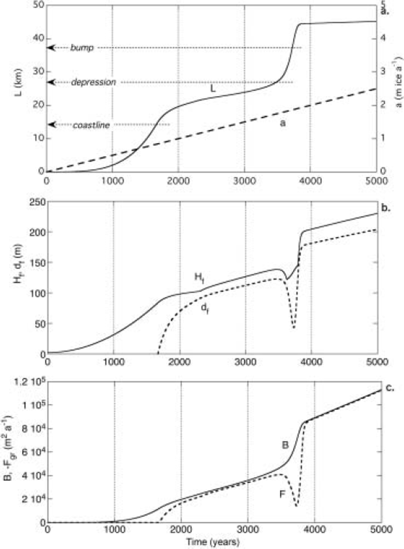
Fig. 2. Results from a calculation in which the accumulation rate increases linearly in time. Panel (a) shows glacier length L and accumulation rate a. Ice thickness and water depth at the glacier front (d f) are shown in panel (b). The components of the mass budget are plotted in panel (c).
Other parameter values related to the physical characteristics of the model glacier are: ε = 1, δ= 1.127, αm = 2 m1/2, α f = 0.7 m1/2 and c = 2.4 a–1. These values should be taken as having the right order of magnitude. Later we will consider the effect of a change in some of these parameters.
The results for this case are summarized in Figure. 2. As expected, the glacier length does not show a steady increase. Until t = 1500 years the glacier is out of balance, because there is no calving to compensate for the accumulation of mass. Then the glacier length increases slowly, and the net mass budget is very small (B + F ≈ 0). When the glacier front approaches the bump in the bed, the mass loss by calving decreases drastically (Fig. 2c) and a rapid change results. The glacier front advances by about 15 km in 200 years. Then the snout enters deeper water and the glacier is in a state of quasi-equilibrium again. To judge the speed of advance in proper perspective, it is important to note that the timescale for the transition to a larger glacier covering the entire submarine bump is a volume timescale, i.e. determined by the change in total ice volume due to the rapid decrease in the calving rate. The present model is not able to simulate a similar advance that could perhaps be initiated by changes in the mechanical properties of the glacier (e.g. enhanced flow due to changing subglacial/hydraulic conditions).
It can be seen that for the particular choice of parameter values, at some point the ice thickness at the front increases significantly above buoyancy because αfL 1/2 becomes larger than -εδd. The very rapid increase in glacier length at t= 3500 years and the large mass imbalance (Fig. 2c) suggest that the model has no stable equilibrium states for a range of values of L. Equilibrium states have been calculated for many parameter values, and some of the results are shown in Figure 3. With a as control parameter, there are two sets of equilibrium states, disappearing at critical points (black dots in Fig. 3). In fact, the critical points are connected by a set of unstable equilibrium states, which are not plotted. The solution diagram implies strong hysteresis (arrows in Fig. 3). Once a large glacier extending into deeper water has formed, a large change in the forcing is needed to jump back to the lower stable branch.
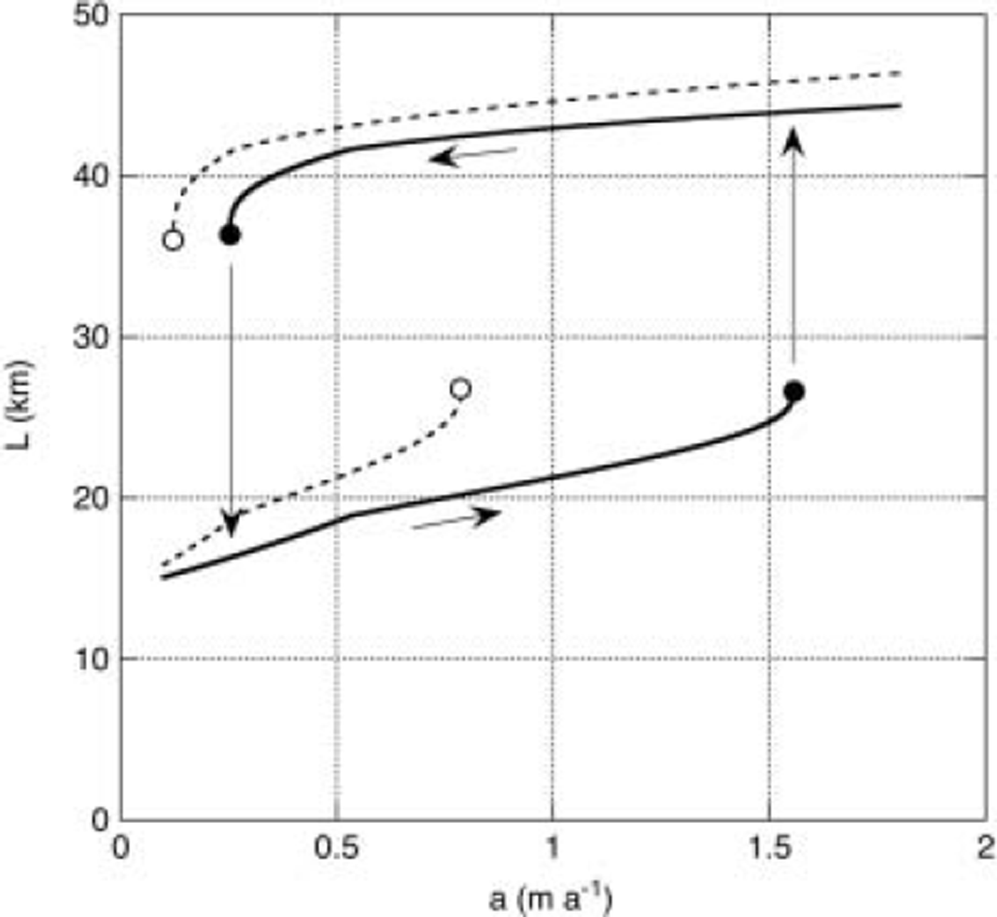
Fig. 3. Solution diagram for the tidewater glacier model with a uniform accumulation rate. Solid lines represent equilibrium states for the reference case (c = 2.4 a–1). Arrows indicate the implied hysteresis. The dashed lines refer to the case in which the calving-rate parameter is halved.
Although the glacier front can advance or retreat over the part of the bed with the reversed slope (db/dx> 0), it cannot attain a stable equilibrium state. This is in agreement with results and inferences made in earlier studies, and gives credibility to the present model. Notably, the model behaviour seen here agrees in a qualitative sense with the results of the comprehensive model of Reference Vieli, Funk and BlatterVieli and others (2001). Unfortunately, Vieli and others did not study solution diagrams of equilibrium states, so a detailed comparison cannot be made.
The non-linear behaviour stems from the dependence of the calving rate on the water depth. Therefore, we expect a strong influence of the calving-rate factor c. The dashed curves in Figure 3 show the equilibrium states in the case that c is halved. Clearly, the ‘width’ of the hysteresis is much smaller now. A similar effect is seen when the amplitude of the bump (λ in Equation (9)) is reduced.
4. The Case of a Mass Balance Depending on Altitude
Many tidewater glaciers are in a warmer climatic environment and have large ablation zones. In this case, it is more appropriate to use Equation (5) as an approximation for the mass balance. This implies that the mean surface elevation enters the equation for mass conservation, and we have to express hm in terms of the other quantities describing the geometry of the glacier. Since we do not want to calculate or specify a surface profile of the glacier, we estimate hm as
Here df is the water depth at the calving front. Equation (10) is easily incorporated in the model. Glaciers in a warmer climate, in which significant melt and runoff takes place, are generally thinner because the ice viscosity is larger and sliding more pronounced, especially in the lower reaches. To mimic this in a primitive way, we set αf = 0.5 m1/2 (instead of α f = 0.7 m1/2 as used in section 2 for the case with a constant accumulation rate and no melting). The balance gradient β was set to 0.005 a-1.
First we consider a calculation with a periodic variation in the height of the equilibrium line, according to
Figure 4 summarizes results for E 0 = 100 m, AE = 350 m and P E = 5000years. These values have been chosen in such a way that the full cycle of glacier initiation, extension across the submarine bump to a maximum length of about 46 km, and retreat is simulated (Fig. 4a). Inspection of the mass-budget components (Fig. 4c) reveals that the glacier is not close to equilibrium when it extends into the sea and crosses the bump. Again, this is related to the inherent dynamics of the model glacier and not to the period of the forcing. Figure 4b provides a further look at the geometry. The ice thickness at the glacier front varies in much the same way as for the case with constant accumulation, of course. The mean ice thickness is proportional to L 1/2 , and therefore behaves more smoothly than the frontal thickness when the glacier crosses the bump.
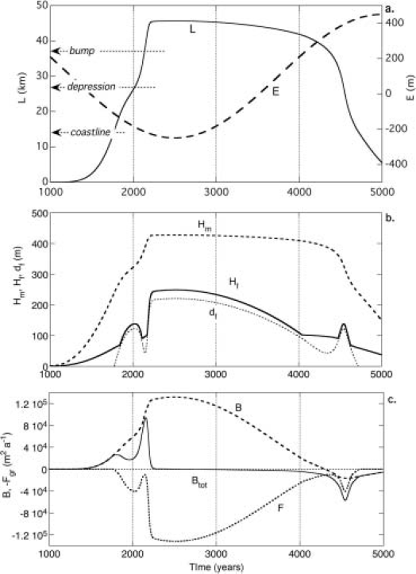
Fig. 4. Results from a calculation with a linear balance gradient and periodic forcing. Panel (a) shows glacier length L and equilibrium-line altitude E. Ice thicknesses and water depth at the glacier front are shown in panel (b). The components of the mass budget are plotted in panel (c).
There is a significant asymmetry between advance and retreat across the bump, reflected in the rate at which the glacier length changes. This rate is smaller for retreat than for advance (although still quite large: ∼5 km in 100 years). The difference is also illustrated by the peak values of the total mass budget (Btot). The (positive) peak value during advance is about twice as large as the (negative) peak value during retreat.
Another set of calculations was done to study the dependence of the solution on the period of the forcing, and to see how the equilibrium states are approached when this period goes to very large values. Results are shown in Figure 5. Glacier length is plotted as a trajectory in the (E,L)-plane. For a forcing period of 50 kyr the trajectory is close to the equilibrium states (cf. Fig. 2), and further increase of the period makes little change.
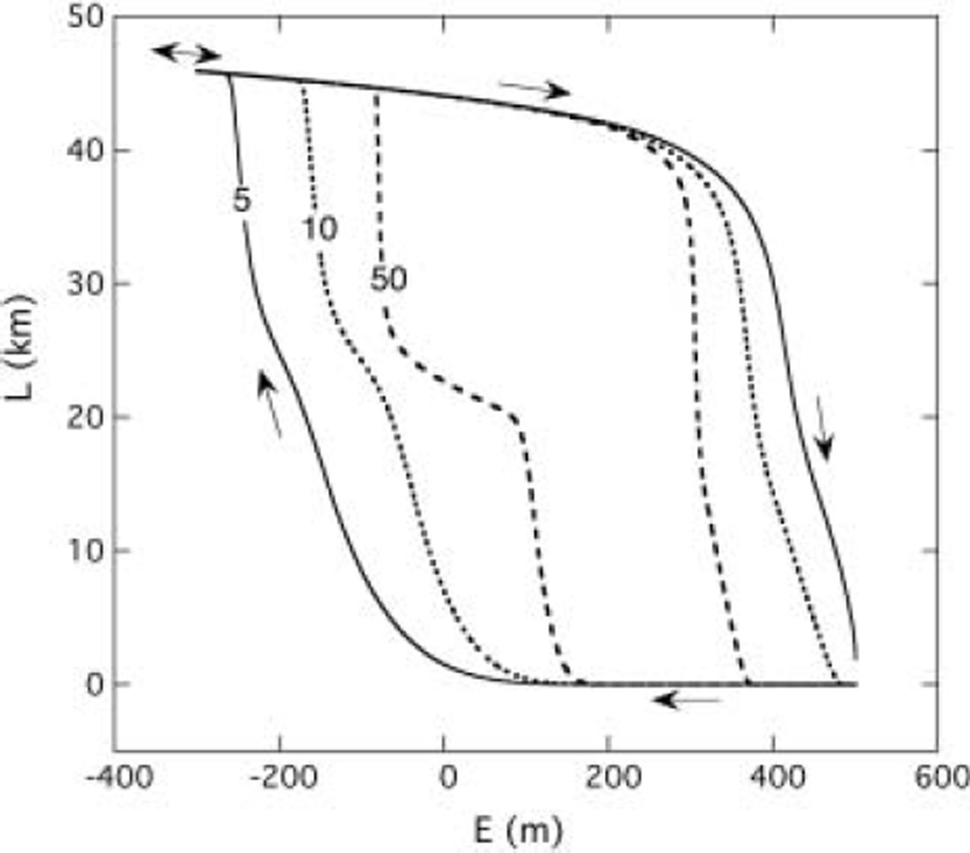
Fig. 5. Glacier length L vs equilibrium-line altitude E for three values of the period of forcing P E (labels in kyr). The model follows a trajectory as indicated by the arrows.
Even when the glacier terminates on land (L< 14 km), the path of advance and retreat in the (E,L)-plane is not the same for the different periods of forcing. This reflects the well-known non-linearity associated with the height-mass-balance feedback (which is absent in the case of constant accumulation). Therefore the full solution diagram contains two regions of hysteresis, one due to the dependence of the calving rate on the water depth (HYS1), the other due to the fact that the mass balance increases with altitude (HYS2). In the case of Figure 5, HYS2 is ‘embedded’ in HYS1. However, as will be demonstrated shortly, for a different bed profile HYS1 and HYS2 can appear as fully separated features in the solution diagram.
The calving-rate parameter c plays a very important role, of course. Figure 6 shows results for different values of c. As expected, the ‘width’ of HYS1 increases with increasing c. The larger the value of c, the more difficult it is for the glacier front to cross the overdeepening in the bed profile. We also observe a weak dependence of the maximum glacier length on c (for a given value of E). The interpretation is straightforward: for a smaller value of c a larger water depth is needed to obtain the mass flux required for equilibrium. From Equations (3) and (4) it can be seen that a change in ε has the same effect as a change in c, so we do not elaborate further on this.
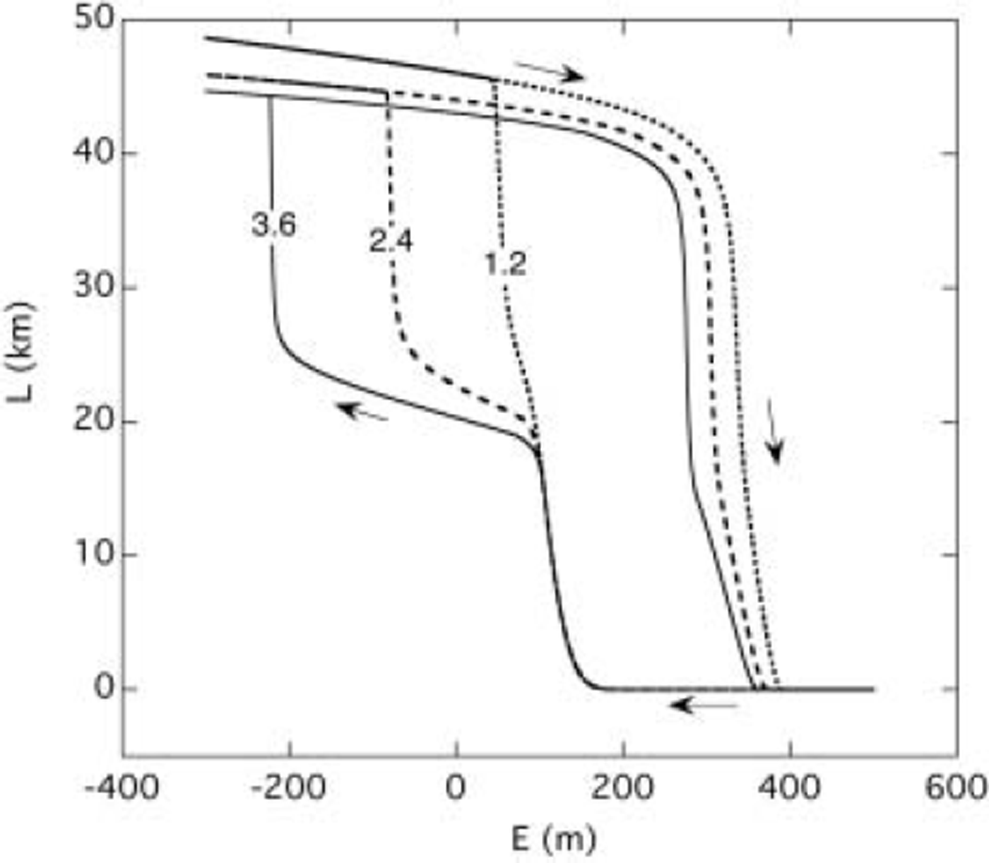
Fig. 6. Glacier length L vs equilibrium-line altitude E for three values of the calving-rate parameter c (labels in a–1). The model follows a trajectory as indicated by the arrows. The forcing period is 50 kyr for all cases.
As mentioned above, it is not difficult to change the bed profile in such a way that HYS1 and HYS2 are separated. Figure 7 shows the stable equilibrium solutions for slightly changed values of d 0 (=320m) and s (=0.019). So the bed is slightly steeper now and it is somewhat higher at x = 0. For values of E between 180 and 320 m there is only one stable equilibrium state.
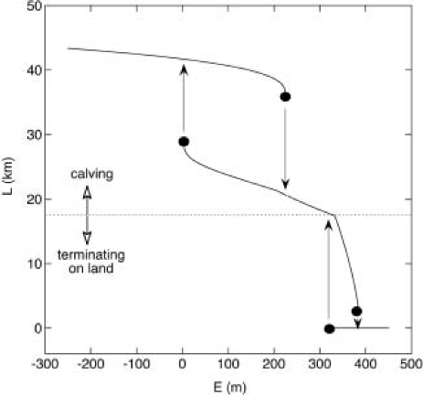
Fig. 7. Equilibrium glacier length L vs equilibrium-line altitude E. Critical points where the solution bifurcates are indicated by black dots. Model parameters are given in the text.
The complexity of the solution diagram depends to a large extent on the bed geometry. In principle, every overdeepening of the bed can lead to branching of the equilibrium states. The response time of the glacier varies enormously, depending on where exactly the glacier is located in the solution diagram.
5. Concluding Remarks
The model described in this paper is simple, yet it has rich dynamics due to the coupling of calving and water depth, on the one hand, and the feedback between mean ice thickness and mass balance, on the other. It appears that these two processes dominate the global dynamics of glaciers on the longer timescales. In spite of its schematic nature, our model reveals the first-order response of glaciers to climate change.
Our approach is based on the belief that on the longer timescales the mass budget determines the dynamic behaviour of a glacier. We have therefore taken the total mass budget as the starting point and have included the mechanical processes in a strongly parameterized way. Here our investigation differs from the more usual approach. Especially for tidewater glaciers, in many earlier studies the focus has been on detailed mechanical processes. These are certainly important to understand the often very rapid and catastrophic events seen at some glacier fronts, which cannot be predicted by our simple model (but can they be predicted anyway?).
We are currently making a comparison between the present simple model and a numerical model in which different parameterizations of the calving process are incorporated. The results of the minimal model and the numerical model are remarkably similar (Nick and Oerlemans, in press). With regard to equilibrium states, all the models show the same dynamic structure; only the locations of the bifurcation points shift slightly. The largest discrepancy between model and reality is probably the ignorance of sediment transfer and lodging during the phase of glacier advance. This shortcoming is common to all models. There is ample evidence that deposition/erosion and transfer of glacial sediments plays an important role and may facilitate greatly the advance of a tidewater glacier (e.g. Reference AlleyAlley, 1991; Reference Van der VeenVan der Veen, 1996). Including such effects in modelling studies, simple or more comprehensive, represents a major challenge for future studies.


