Introduction
Snow cover is frequently heterogeneous on length scales too small to be resolved by a general circulation model (GCM) grid, introducing marked sub-grid heterogeneities in land-surface characteristics and fluxes. A high-resolution two-dimensional (2-D) boundary-layer model is used in this study to model turbulent fluxes of heat and moisture over heterogeneous snow cover. The performance of a “tile” model, which parameterizes gridbox-average surface fluxes as weighted averages of fluxes over snow-covered and snow-free regions, is assessed in comparison with the boundary-layer model. Using the tile model to allow for heterogeneous snow cover in a single-column version of the Hadley Centre GCM is found to have a large impact on the partitioning of available energy into latent and sensible heat fluxes.
The Boundary-Layer Model
The boundary-layer model used here is described by Reference Wood and MasonWood and Mason (1991). Velocity components, potential temperatures and specific humidities are found as solutions of the Boussinesq equations with first-order turbulence closure on a 2-D grid that has a horizontal spacing of 31.25 m and 20 vertical levels (five in the lowest 10 m) extending up to 5000 m. The numerical scheme used is second-order accurate, and energy conserving. Vertical fluxes of heat and moisture are set to zero at the upper boundary, and the flow is driven by a constant horizontal-pressure gradient. Periodic boundary conditions are imposed at the left-hand and righthand edges of the model domain, which is 1 km wide.
Parameterizations of surface radiation, sensible heat and moisture fluxes have been added to the boundary-layer model (Reference EsseryEssery, in press). Sensible heat fluxes (H) and moisture fluxes (E) are proportional to differences in potential temperature (θ) and specific humidity (q) between the surface and the lowest model level (at height z = 0.25 m), divided by appropriate resistances;

and

where θ0 is the surface potential temperature, qsat(T0) is the saturation humidity at surface temperature T0, and rs is a surface resistance for moisture transfer (zero for saturated surfaces such as snow). The aerodynamic resistance, ra, increases with increasing atmospheric stability, decreasing surface roughness (characterized by roughness length z0 ) and decreasing windshear, all of which suppress turbulent transport.
Given downward fluxes of solar and longwave radiation (SW↓ and LW↓ ) and assuming unit longwave emissivity, the net radiation at a point on the surface is
where α is the surface albedo, and σ is the Stefan Boltz-mann constant. The net radiation is partitioned into sensible, latent, ground and snowmelt heat fluxes. Surface temperatures are found by inverting the surface-energy balance,
The sign convention used is that R and G are positive downward, and H and E are positive upward. Hsm is the snow-melt heat flux required to ensure that the calculated snow-surface temperature does not exceed 0°C, G is the ground heat flux (assumed to be negligible) and λ is taken to be the latent heat of sublimation at snow-covered points or the latent heat of vaporization at snow-free points.
The boundary-layer model was run with surface parameters, shown in Table 1, chosen to represent forest, grass and snow-covered grass. The snow is given the same roughness length as the grass (roughness lengths for deep, continuous snow covers are generally much lower) but has higher albedo and zero surface resistance, whereas the forest has the same albedo as the grass but larger roughness length and surface resistance. It should be noted that the drag at model levels that would lie within the forest canopy is not explicitly represented, and the modelled wind profile is only valid at heights above the canopy.
Table 1. Surface parameters for forest, grass and snow-covered grass

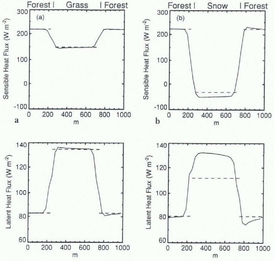
Figure 1a shows heat fluxes across a surface with 500 m fetches of forest and grass, homogeneous downward radiation fluxes (SW↓ = 400 W m−2 and LW↓ = 300 W m−2) and a 10 m s−1 geostrophic wind blowing from left to right. The sensible heat flux is higher and the latent heat flux is lower over the forest, but both are upward everywhere, and the energy available to be partitioned into latent and sensible heat fluxes is nearly homogeneous across the surface. Replacing the grass by snow gives similar latent heat fluxes, as shown in Figure 1b, but the high albedo of the snow gives a lower available energy, requiring the sensible heat flux to change direction from upward over the forest to downward over the snow. Heat is advected from the warm forest to the cold snow, and a shallow, stable internal boundary layer forms over the snow. The stable layer is capped by an inversion in the local temperature profile, which reaches a height of 13 m at the downwind edge of the snow patch in this case. Advection over heterogeneous snow has been studied by Reference ListonListon (1995) using a similar modelling strategy.

Fig. 1. Surface sensible and latent heat fluxes for (a) forest and gray, and (b) forest and snow. Solid lines are from the boundary-layer model and dashed lines are from the tile model.
The Tile Model
GCMs require parametefizations to calculate gridbox-average fluxes given gridbox-average temperatures, humidities and windspeeds at a reference height in the atmosphere. Local fluxes, however, depend non-linearly on local vertical gradients, and average fluxes are not simply related to average gradients over heterogeneous surfaces. It has been suggested that surface heterogeneity can be represented by gathering distinct surface types within a gridbox into homogeneous “tiles” and calculating fluxes separately over each tile (Reference Avissar and PielkeAvissar and Pielke, 1989; Reference ClaussenClaussen, 1991).
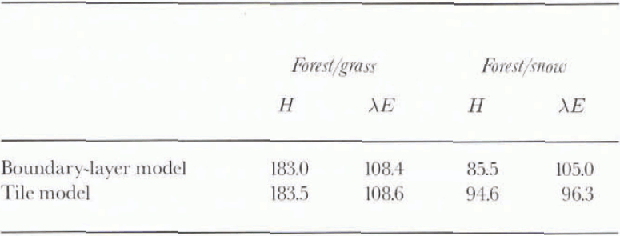
A tile model, using the same surface-flux parameterizations as the boundary-layer model and driven by area-average data from the boundary-layer model at a height of 19 m (typical of the lowest atmospheric level in a GCM, but too high to resolve the shallow, stable layer over the snow), has been assessed in comparison with the boundary-layer model by Reference EsseryEssery (in press). As shown by Reference Blyth, Dolman and WoodBlyth and others (1993), a tile model can work well for heterogeneous vegetation. The dashed lines on Figure 1a show fluxes calculated for forest and grass tiles. The tile model does not represent advective effects at the edges of the forest and grass patches, but it does give very good values for average fluxes in this case (Table 2). Figure 1b shows that the performance of the tile model is degraded for forest and snow as a result of the large variation in stabilily across the surface; the magnitudes of the fluxes over the snow tile are underestimated, giving an overestimate of the average sensible heat flux and an underestimate of the average latent heat flux (Table 2). Nevertheless, the tile model captures the change in stability between forest and snow, and still estimates the average fluxes to within about 10%. A slight improvement in the partitioning of the available energy over the snow tile can be achieved by using windspeeds on a separate reference height from temperatures and humidities (Reference EsseryEssery, in press).
Table 2. Average sensible and latent heat fluxes (W m−2) from the boundary-layer model and the tile model

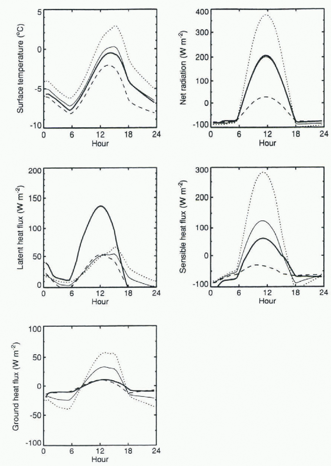
As a first step towards a GCM implementation, a tile model of heterogeneous snow cover has been tested in a single-column version of the Hadley Centre GCM. Unlike the boundary-layer model, the GCM uses a soil model to calculate ground-heat fluxes. Figure 2 shows surface temp-eratures and fluxes during one day for a model gridbox with 50% snow-covered grass; the snow-free fraction is forested, as in the boundary-layer model. The forest (dotted lines) absorbs much more radiation and has a higher temperature than the snow (dashed lines). Latent heat fluxes from the snow and the forest are comparable, although the evaporation peaks later in the day over the forest than over the snow. The sensible heat flux over the snow is small and downward throughout the day, but there is a large, upward flux from the forest around midday that dominates the gridbox-average sensible heat flux (thin solid line). The ground heat flux is very small (less than 3 W m−2), when averaged over 24 hours, but gives a fairly strong warming for the forest fraction during the day and cooling at night.

Fig. 2. Gridbox-average surface temperatures and fluxes obtained using a tile model (thin lines) and effective surface parameters (thick lines) in a single-column version of the Hadley Centre GCM. Dotted and dashed lines show values for forest and snow tiles respectively.
Most current GCM land-surface schemes do not calculate separate fluxes for snow-covered and snow-free fractions of a gridbox — CLASS (Reference VerseghyVerseghy, 1991) is an exception — but instead use “effective” surface parameters to relate gridbox-average fluxes to gridbox-average gradient. Thick lines on Figure 2 show results obtained from the single-column model with the following parameter choices. Assuming the snow to be uniformly distributed across the gridbox. the surface resistance is set to zero. Simply using the average albedo (α = 0.5) gives the correct average net surface shortwave radiation. The roughness length is set to the log average of the local roughness lengths (z0 = 0.1 m), the effective value predicted by linear theory for small variations in roughness. The effective parameter model gives nearly the same surface temperature and net radiation as the tile model, but the partitioning of the available energy is changed; the peak latent heat flux is higher and the peak sensible heat flux is lower.
Conclusions
Although the tile model performs less well in situations with large sub-grid variations of stability, it still gives reasonable estimates of average and local fluxes over heterogeneous snow cover. However, the tile model has only been assessed in comparison with a boundary-layer model that uses the same surface flux parameterizations, and tile model fluxes have not been compared with fluxes measured over real surfaces.
The explicit representation of heterogeneities in snow cover is likely to have large impacts on GCM surface fluxes. For a complete parameterization of heterogeneous snow-cover, the problem of determining a closure relating fractional snow coverage to surface characteristics and average snow depth remains.
Acknowledgements
N. Wood supplied the boundary-layer model. P. Rowntree, J. King and an anonymous referee made a number of useful comments in reviewing this paper. This work was supported by the U.K. Department of Environment.


