Sea-ice model validation using submarine measurements of ice draft

Abstract

Sea-ice thickness distributions from 12 submarine cruises under the North Pole are used to evaluate and enhance the results of sea-ice model simulations. The sea-ice models include versions with cavitating fluid and elastic-viscous-plastic rheologies, and versions with a single thickness and with multiple (5–27) thicknesses in each gridcell. A greater portion of the interannual variance of observed mean thickness at the Pole is captured by the multiple-thickness models than by the single-thickness models, although even the highest correlations are only about 0.6. After The observed thickness distributions are used to ˚tune" the model to capture the primary mode of the distribution, the largest model-data discrepancies are in the thin-ice tail of the distribution. In a 41 year simulation ending in 1998, the model results show a pronounced decrease of mean ice thickness at the Pole around 1990; the minimum simulated thickness occurs in summer 1998. The decrease coincides with a shift of the Arctic Oscillation to its positive phase. The smallest submarine-derived mean thickness occurs in 1990, but no submarine data were available after 1992. The submarine-derived thicknesses for 1991 and 1992 are only slightly smaller than the 12–case mean.

1. Introduction

The modeling of large-scale sea-ice variations has been an active area of research for the past several decades. With the increased awareness that sea ice may be instrumental in climate change over the next several decades, sea-ice modeling has taken on added importance in studies of the climate system. While the areal coverage (or extent) of sea ice has generally received the most attention in global-climate model simulations, primarily because changes in areal coverage trigger the albedo-temperature feedback, the areal coverage alone does not provide a measure of the volume or mass of sea ice. Ice volume provides the most direct measure of the amount of sea ice present, the amount of melting required to eliminate the sea ice and, to a good approximation, the amount of salt that has been input to the ocean as rejected brine.

Unfortunately, model simulations of sea-ice thickness are difficult to verify because (1) in situ measurements are sparse, and (2) satellite remote-sensing techniques for the determination of ice thickness have proven to be elusive. The available database of in situ measurements is limited largely to time series of a few years from moored sonars that have been deployed in relatively shallow waters over the past decades, and to the relatively small set of declassified sonar measurements from submarine cruises. The sparse database of submarine sonar data has been used by Bourke and Garrett (1987) to construct an ice-thickness climatology for the Arctic Ocean and by McLaren and others, (1992), Wadhams (1994) and several others to illustrate the interannual variations of ice draft at particular locations (e.g. the North Pole).

In the present paper, we take the submarine sonar data one step farther by using them to verify and to guide improvements in model simulations of Arctic sea ice. Conversely, model simulations can point to priorities in the spatial and temporal sampling of a variable such as ice thickness. We will show that the need for ice-thickness data for particular time periods and regions emerges from the model results presented here. In the case of sea-ice thickness, the model results suggest data priorities with respect both to the past, since existing data are available for declassification, and to the future, since cruises and mooring deployments can be planned more effectively when specific needs have been identified.

2. Ice-Thickness Data

The ice draft measurements used here are from 12 cruises of United States Navy STURGEON-class submarines that crossed beneath the geographic North Pole during the 1977–92 period. The submarines operated upward-looking active sonars that provide measurements of ice draft (vertical distance from ocean surface to ice underside) when referenced to areas of open water (zero draft). The declassified data are for a small area within 150 km of the North Pole. The corresponding transit time was typically 1–2 days. Eight of the twelve cruises passed under the Pole during the spring months of April-May The remaining cruises passed under the Pole during the autumn months of September-November. Although the cruises are distributed throughout the 1977–92 period, two gaps stand out in the data record: there are no declassified cruise data between spring 1979 and autumn 1982, nor for the period between autumn 1982 and spring 1986. One year, 1990, had both a spring and an autumn cruise.

The ice-draft measurements from these cruises were available as histograms, typically containing several tens of thousands of draft measurements, processed by Arctic Analysts, Inc. (Boulder, CO) into 10 cm bin widths. The histograms can be used to evaluate mean drafts, as described by McLaren and others (1992) and Shy and Walsh (1996). The mean drafts for these 12 cruises ranged from approximately 2.4 m (autumn 1990) to approximately 5.5 m (spring 1979).

We note here that ice draft is generally about 12% smaller than ice thickness (Barry and others, 1993), which is the corresponding variable computed by sea-ice models. For model-data comparisons, one may reduce the ice thicknesses by 12% for a comparison of ice drafts, or increase the drafts by 12% for a comparison of thicknesses. In this study, we follow the latter approach in the model-data comparisons.

3. Model Simulations

Several sea-ice model simulations were made of multi-decadal periods that included the 1979–92 time-frame of the available submarine data. We tested two different ice rheologies, as well as a single-level formulation and a multilevel formulation of ice thicknesses. The use of these different model versions permitted a comparison of their simulations of the interannual variations present in the sonar-derived ice thicknesses in terms of both the mean thicknesses and (in the case of the multilevel simulations) the thickness distributions.

All versions of the model included the same thermodynamic parameterization, which consists of a surface energy budget computation following Parkinson and Washington (1979) and modified by Walsh and Zwally (1990). The sensible- and latent-heat flux computations follow Ebert and Curry’s (1993) use of bulk transfer coefficients for open ocean and ice surfaces modified according to the stability of the near-surface environment. In the multiple-thickness simulations, a different coefficient is determined for each thickness category of ice in a gridcell.

The treatment of ice dynamics is based on a momentum balance equation. The two different forms of the ice rheology in the internal ice-stress term are the cavitating fluid (CF) formulation of Flato and Hibler (1992) and an elastic-viscous-plastic (EVP) formulation (Hibler, 1979; Hunke and Duko-wicz, 1997). These formulations are essentially the same as those used in the Sea-Ice Model Intercomparison Project (Kreyscher and others, 1997). Both were used here in simulations with a single (time-dependent) ice thickness in each gridcell. The EVP rheology was then used with a multilevel ice-thickness formulation (Flato and Hibler, 1995). The multilevel formulation allows for the representation of each grid-cell’s ice cover in terms of a thickness distribution containing a user-prescribed number of thickness categories or ˚bins". This thickness distribution permits direct comparisons between the model output and the draft distributions from the submarines.

Two key parameters in Flato and Hibler’s (1995) multiple-thickness formulation are H*, which controls the size of the ridges and also the number of ridges required to accommodate a given deformation, and C_1, which controls the range of ice thicknesses that participate in ridge-building. As described in the following section, the model-data comparison led us to modify the values of both these parameters.

The forcing data for the multiple-thickness simulations were obtained from the U.S. National Center for Environmental Prediction (NCEP)/National Center for Atmospheric Research (NCAR) re-analysis (Kalnay and others, 1996), which spans the period 1958–98. For the single-level CF and EVP simulations, the forcing from 1979 onward was based on the Arctic Ocean Buoy Program’s gridded fields of sea-level pressure and the POLES (Polar Exchange at the Sea Surface) air temperatures (Martin and Munoz, 1997). For the 1951–78 period, the CF and EVP simulations used sea-level pressure (SLP) grids from NCAR and air-temperature grids from Chapman and Walsh (1993). These forcing data were used instead of the NCEP/NCAR re-analyses for the single-level simulations because they were the best forcing available at the time these simulations were performed. There is significant overlap between the two datasets and we have found no evidence of major differences in the two sets of SLP grids nor in the post-1979 temperature grids. However, the pre-1979 temperatures from the reanalysis contain more interannual variance than those from Chapman and Walsh (1993).

The model’s ocean currents were temporally invariant and were computed geostrophically from Coachman and Aagaard’s (1974) dynamic topography. Thermodynamically, the ocean was treated as a 30 m mixed layer with a spatially and temporally invariant heat flux of 2.0 W m–² from the underlying ocean.

All simulations began in the 1950s in order to ensure an adequate spin-up prior to the sonar-data comparison period, which began in 1977. For all multiple-thickness simulations, the thickness distributions were initialized with output from a prior multi-decadal simulation that ended in 1998. The single-level CF and EVP simulations began with an ice-free Arctic in January 1951. All simulations were run on a Cartesian grid with a resolution of 110 km for the single-thickness runs and 100 km for the multiple-thickness runs.

4. Model Results and Comparison to Data

The simulated ice thicknesses were averaged over the four model gridpoints within 150 km of the North Pole for a direct comparison to the submarine-derived thicknesses (drafts × 1.12) on the 12 cruise dates. For each model, the simulated velocities at the North Pole were ˚tuned" to match the observed ice velocities obtained from the nearest buoy in the International Arctic Buoy Program archive. In the case of the single-level CF model, this required an almost 50% reduction in simulated pole velocities, implying that the untuned CF drift speeds were too fast by about a factor of two. For the CF model, we decreased the model velocities by increasing the ice-strength and ocean-drag coefficients. The EVP model needed only minor adjustments in the same direction. For the multiple-thickness simulations, we reduced the simulated velocities slightly by increasing the ice-strength and ridging-participation parameter and decreasing the maximum ridge-height parameter. Next, the simulated mean thicknesses were tuned by adjusting the minimum lead fraction and the surface exchange coefficients until the 12–case mean thickness of the models was within 10% of the 12–case mean thickness from the submarine measurements. (The ˚tuning" kept all parameters within the published ranges of their observational estimates.) While results from the ˚base" simulations as well as the ˚tuned" simulations for the single-level models will be summarized later, we show in Figure 1 the 12 individual thickness anomalies from the submarine measurements and the corresponding 12 thickness anomalies from the ˚tuned" CF and EVP simulations.

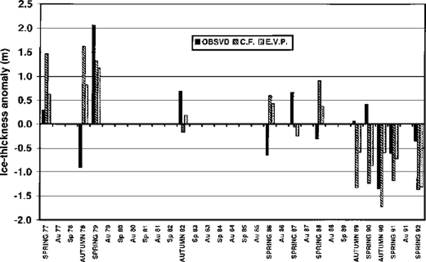
Fig. 1 Mean ice thickness at North Pole as measured by submarine sonar (left-most bars, solid), simulated by CF model (center bars, striped) and simulated by EVP model (rightmost bars, stippled).

It is apparent from Figure 1 that the models’ thicknesses are considerably larger than the submarine measurements in some cases (e.g. autumn 1978, spring 1986) and considerably smaller than the submarine measurements in other cases (e.g. autumn 1989, spring 1990). The correlations between the simulated and observed thicknesses are 0.31 for the CF simulation and 0.36 for the EVP simulation. The corresponding root-mean-square (rms) errors are 1.26 m (CF) and 0.95 m (EVP), indicating that the single-level EVP model was somewhat more successful at capturing the interannual variations. The more noteworthy finding is that neither simulation captured more than 15% of interannual variance of the sonar-derived mean thicknesses. The EVP model nevertheless produced its largest thickness of the 12 values in the same case (spring 1979) in which the submarine thickness reached its largest value.

In order to assess the relative importance of the dynamic and thermodynamic forcing in producing the interannual variations, two additional simulations were made with the CF model. In one (the ˚dynamics-active" simulation), all air temperatures were replaced by seasonally varying climatological values, while in the other (the ˚thermodynamics-active" simulation) the sea-level pressures and wind-forcing were replaced by their climatological counterparts. For 11 of the 12 observational cases, the dynamics-active simulation produced a more accurate estimate of the sonar-derived thickness than did the corresponding thermodynamics-active simulation. The linear correlations with the observed thicknesses were 0.46 and 0.13 for the dynamics-active and thermodynamics-active simulations, respectively. The corresponding rms errors were 0.87 m and 1.13 m. Subsequent examination of the forcing grids showed that the surface air temperatures were essentially climatological prior to 1979, even in the thermodynamics-active simulation. Although the thermodynamics-active simulation was disadvantaged in this respect, the fact remains that the dynamics-active simulation showed a better correlation with the observed drafts than did the complete ("all-processes-active") simulation. We conclude that the dynamical processes made the greater contribution to any success of the single-level CF model in capturing the observed variations of ice thickness at the Pole.

The multiple-thickness simulations were run with five thickness categories (the ˚five-category" simulation) and with twenty-seven categories (the ˚27–category" simulation).

In both cases, the thickness categories had finer resolution at the thin-ice end of the spectrum. Figure 2 shows the observed thicknesses and the corresponding simulated values for the untuned and tuned versions of the five-category simulation. The tuning consisted of a 5% increase of the turbulent transfer coefficients for sensible and latent heat under unstable conditions (T_sfc ≥ T_air) and a 5% decrease under stable conditions. These changes effectively decrease the surface heat loss over leads and thin ice in winter and decrease the surface-heat gain in summer, thereby increasing the ice thickness. The increase of thickness is indeed apparent in the ˚tuned" results of Figure 2. The modified flux parameterization was particularly effective in reducing the excessive loss of ice in autumn 1990 in the untuned simulation.

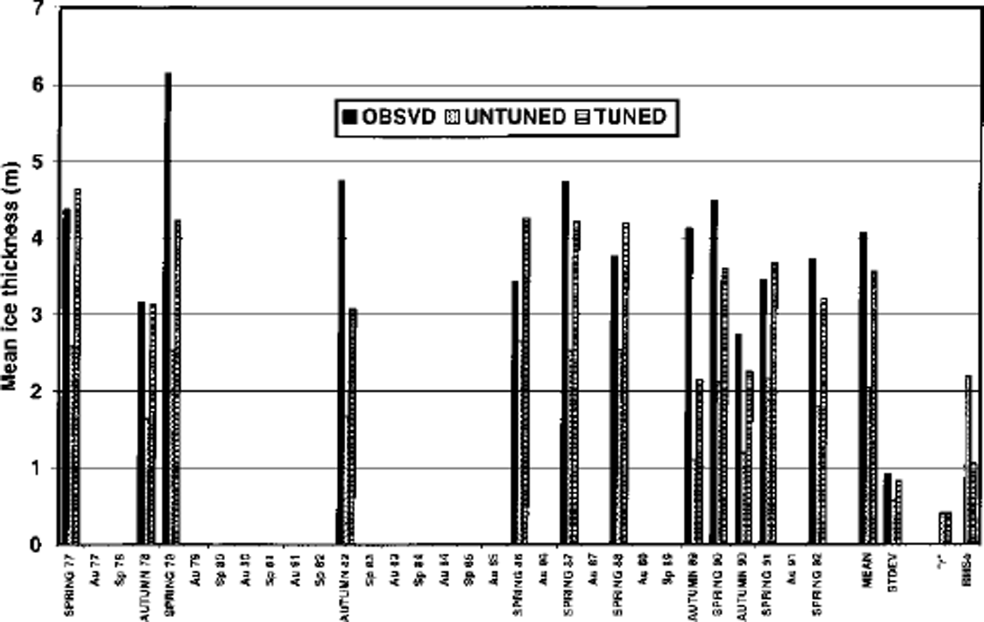
Fig. 2. Mean ice thickness at North Pole as measured by submarine sonar (left-most bars), simulated by untuned five-category model (center bars) and simulated by tuned five-category model (right-most bars).

The correlation between the simulated and observed interannual variations is τ = 0.41 in the tuned five-category simulation, and it increases to τ = 0.59 when the number of thickness categories is increased to 27. The stronger correlation in the 27–category simulation indicates that a more detailed treatment of ice redistribution improves the model’s ability to capture interannual variability in gridcell mean thicknesses. Figure 3 is a scatter plot of the simulated and observed thicknesses in the 27–category simulation. While the range of the simulated thicknesses is somewhat smaller than the range of the measured values, the model and the observations both identify the same case (autumn 1990) as the thinnest and the same case (spring 1979) as the thickest.

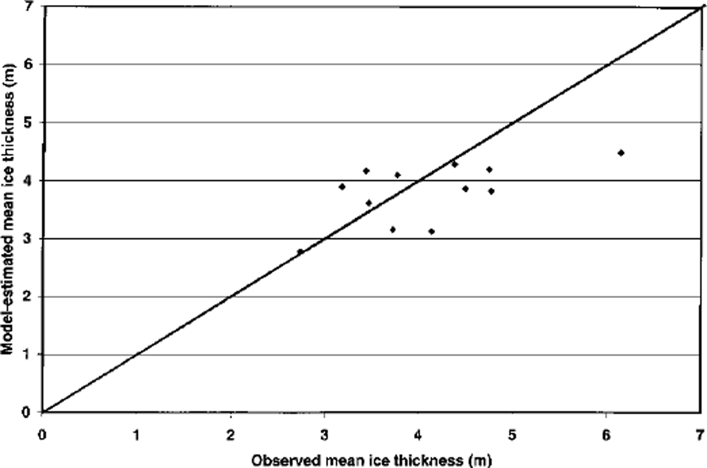
Fig. 3. Scatter plot of observed and model-simulated mean ice thicknesses at North Pole on dates of submarine underpass. Model results are from 27–category tuned simulation. Diagonal line represents perfect agreement between observed and simulated values.

Figure 4 summarizes the discrepancies between the measured thicknesses and the various simulations discussed thus far. The correlations range from slightly negative (untuned CF) to approximately +0.60, while the rms errors range from a ˚worst case" of 2 m (untuned EVP) to a ˚best case" of 0.75 m (27–category). Because the 27–category simulation clearly shows the best agreement with the measured thicknesses, the remainder of the discussion will focus on the 27–category simulation and its thickness distributions.

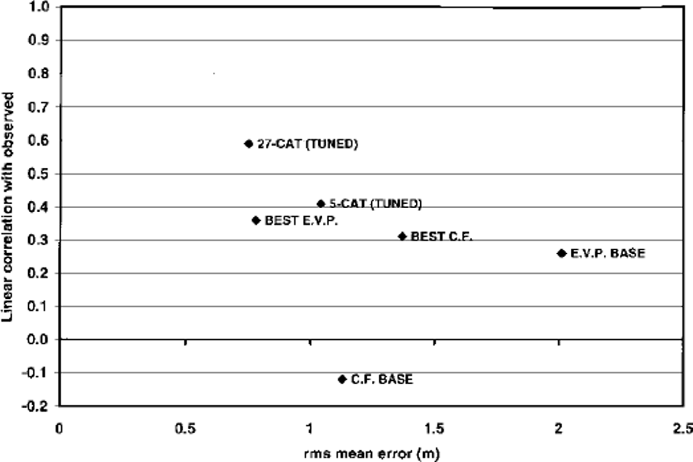
Fig. 4. Summary of the various model simulations’rms errors (m) and linear correlations with observed thicknesses. ˚BASE" indicates "untuned", ˚BEST" indicates ˚tuned".

Figure 5 shows the North Pole ice-thickness distribution through the 41 years (1958–98) of the 27–category simulation. An annual cycle is detectable, as the thicker ice predominated in the late winter and early spring. In most years, thin ice (refrozen open water) appears in late summer/early autumn, after which time its thickening by freezing and subsequent ridging is apparent in the upward and rightward tilt of the ˚spikes" in the lower portion of Figure 5’s color plot. The most pronounced and widespread spikes, indicative of the greatest summertime fractions of open water, appear in the 1990s. Such features appear infrequently in the earlier decades. Another characteristic of the 1990s in Figure 5 is the reduction of thick ice, especially in the autumn.

Fig. 5. Time history of probability density function of ice thickness at North Pole in 27–category model simulation. Deepest reds denote thickness ranges having largest fractions of areal coverage; y axis is non-linear in actual thickness but linear in number of thickness categories containing thinner ice.

Figure 6a shows a time series of the mean ice thickness at the Pole in the 27–category simulation. A strong annual cycle, with a seasonal range of nearly lm, is apparent throughout the time series. This range is larger than the 40–50 cm obtained for a homogeneous slab of multi-year ice in earlier modeling studies dating back to Maykut and Untersteiner (1971) but comparable to the seasonal range in other multiple-thickness sea-ice models (Rothrock and others, in press). In agreement with Figure 5, the time series of mean thickness in Figure 6 shows a substantial decrease in 1990–91. The simulated ice appears to have been unable to recover from this thinning, although the thickness appears to have stabilized at the lower level during the early to mid-1990s. In a recent analysis of submarine-derived ice drafts near the North Pole, Rothrock and others (in press) found a similar 1.5 m decrease in drafts from cruises for the 1958–76 period and colocated drafts measured in the 1990s. The model’s thickness did reach a new minimum in the summer of 1998, coinciding with the Surface Heat Budget of the Arctic Ocean (SHEBA) field measurements of thin ice approximately 1200 km to the south in the Alaskan sector.

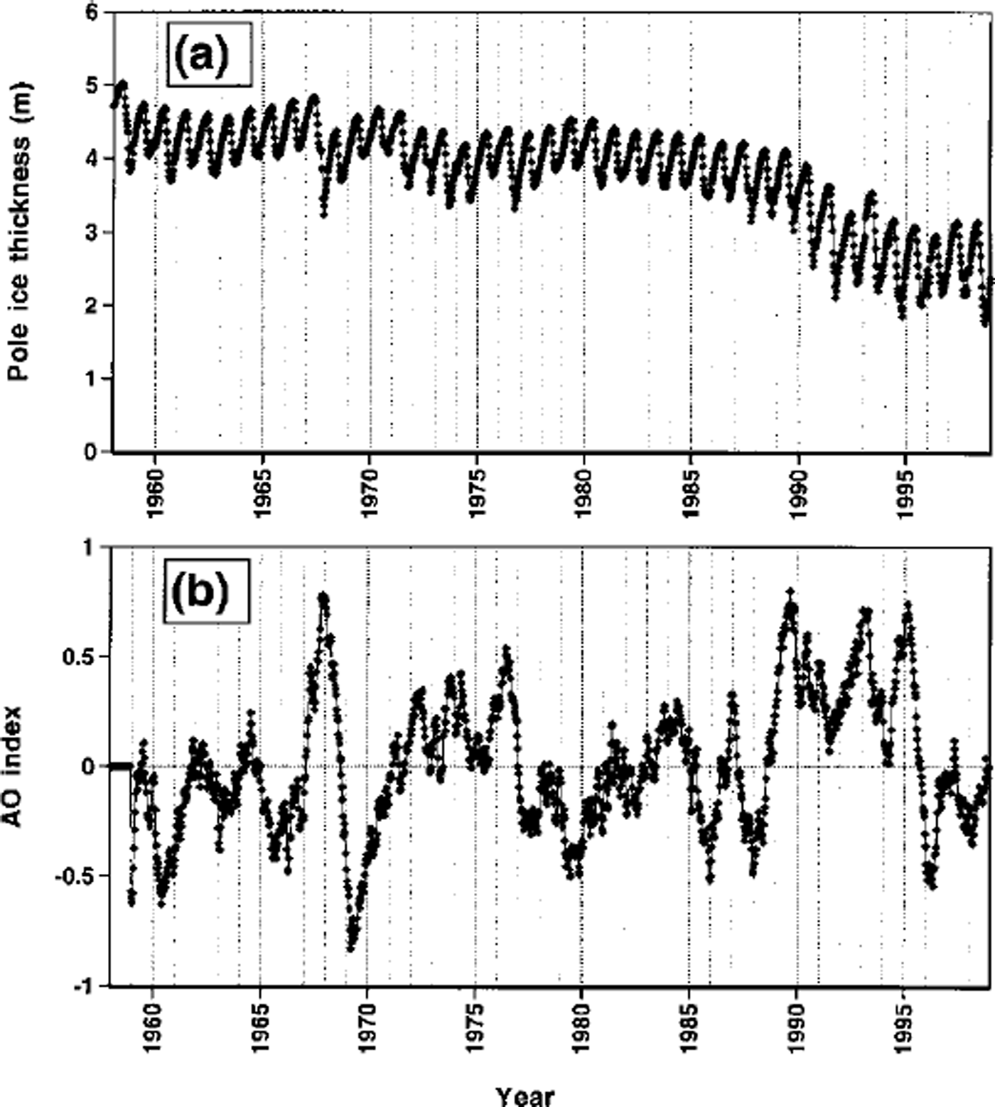
Fig. 6. Time series (1958–98) of (a) monthly ice thickness at North Pole as simulated by 27–category model, and (b) 12 month running mean of AO, defined as difference between monthly sea-level pressure anomalies over Arctic Ocean (70–90° N, 90–270° E) and in North Atlantic subtropical high.

A possible explanation for the temporal behavior of the North Pole ice thickness is shown in Figure 6b, which is a time series of an"Arctic Oscillation" (AO) index of sea-level pressure anomalies. This index, defined here as the difference between the anomalies of sea-level pressure in the central Arctic and the subtropical North Atlantic, is a measure of the intensity of the large-scale teleconnection pattern identified by Thompson and Wallace (1998). The high-index (positive) phase of this index occurs when sea-level pressures are anomalously low in the central Arctic and anomalously high in the subtropical North Atlantic. The increase of this index during 1989–90 coincides with the decrease of ice thickness in Figure 6b. The high AO values in the early to mid-1990s coincide with the persistence of small ice thicknesses through this period. A short-term positive excursion of the AO occurred in 1967–68, at which time a short-lived decrease of ice thickness is apparent in Figure 6a. The implication of Figure 6 is that the large-scale pattern of wind-forcing is a major determinant of ice thickness near the North Pole and perhaps over a wider area of the Arctic. Kwok and Rothrock (1999) have already shown that the AO’s more regional counterpart, the North Atlantic Oscillation, is correlated positively with sea-ice export from the Arctic to the North Atlantic. An outstanding issue is the future course of the AO, at least over the next several decades. The model simulations examined here suggest that the state of this circulation mode may play a greater role in changes of sea ice over the coming decades than will the direct manifestations of greenhouse warming.

In order to evaluate more directly the simulated distributions of ice thickness at the Pole, Figure 7 shows the probability density functions (measured vs simulated) for three cases: spring 1977, autumn 1989 and spring 1991. In each of these cases (and in the nine others), the observed distribution has a sharper peak than the simulated distribution. Thus the model appears to be simulating a broader range of thicknesses, while the measured thicknesses are more concentrated near their modal values. In the case of spring 1977, the model’s peak is clearly to the right of the measured peak, indicating that the model’s ice is generally too thick. In autumn 1989, both the measured and simulated distributions have secondary peaks in the thin ice (<1 m), indicative of recent refreezing of leads or other open water. However, the model’s peak is at 0.0–0.1 m, while the measured peak is at 0.5–1.0 m.Thus the refreezing process is farther advanced in the observational data. In spring 1991, there is more thin ice in the observed distribution, indicating a greater presence of refrozen leads than has been captured by the model.

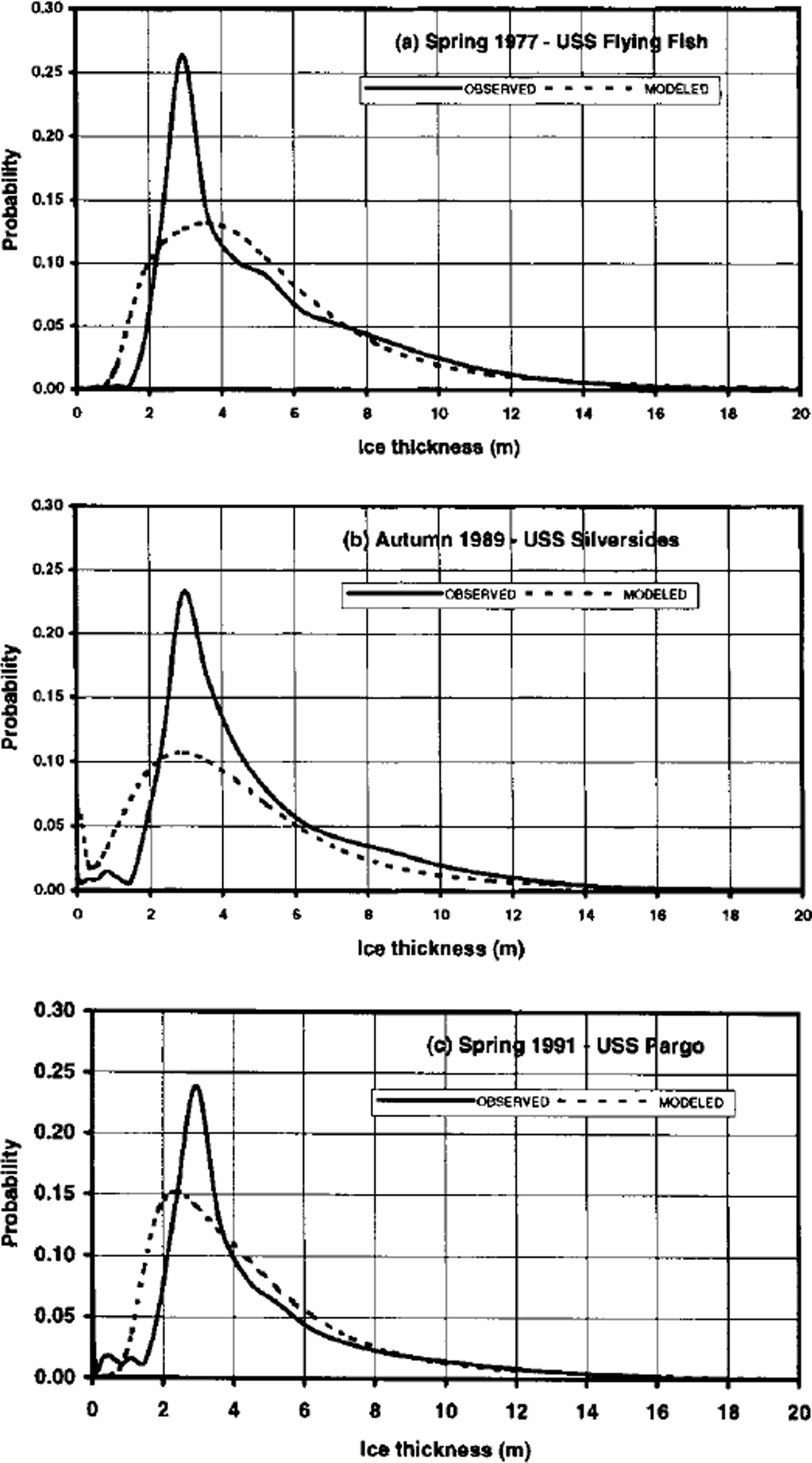
Fig. 7. Probability density functions for North Pole ice thickness measured by submarines (solid line) and simulated by 27–category ice model (dashed line). Results are shown for submarine cruises in (a) spring 1977, (b) autumn 1989 and (c) spring 1991.

In an attempt to use the model-data comparison of thickness distributions to guide model improvements, we addressed the excessive breadth of the simulated distributions by making two physically plausible changes to the model parameterization of thickness redistribution in response to deformation. First, the ridge-height parameter, H*, was doubled from 50 to 100. Second, the ridging-participation parameter, C₁ was reduced from 0.2 to 0.1. These modifications are closer to the optimum values determined by Flato and Hibler (1995). However, they do slightly decrease the correlations of simulated ice velocities with observed buoy-drift velocities in our simulations, at least at the North Pole. As shown in Figure 8, these changes narrow the thickness distributions considerably, thereby improving the agreement with the measured distributions. The shape of the major feature of the spring 1977 distribution in Figure 8 is a good replica of its submarine-derived counterpart, although the model’s distribution is shifted somewhat towards the thin-ice part of the spectrum. The model distributions for the autumn cases suggest that the simulated freeze-up is delayed relative to the observations. Hence additional tests involving the thermodynamics as well as the dynamics appear to be warranted.

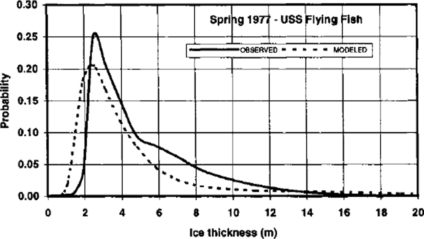
Fig. 8. As in Figure 7a, but with the model results from a simulation in which ridging parameters were tuned (see text).

5. Conclusion

The ice-thickness distribution data from 12 submarine cruises under the North Pole have permitted the testing and improvement of sea-ice model simulations spanning several recent decades. The most notable findings are:

The model-data comparison revealed biases in the model’s mean thicknesses at the Pole; these biases were largely eliminated by adjustments to the model’s thermodynamic parameters. The agreement between the simulated and observed thickness distributions, on the other hand, was improved by adjustments to the parameters used in the redistribution of thickness by ridging.

A greater portion of the interannual variance of North Pole ice draft is captured by the multilevel thickness model than by the models with a single thickness at each gridpoint, although the ˚best" correlations of approximately 0.6 represent explanations of less than half the variance. The simulations described here have not included oceanic variability, nor has their thermodynamic forcing included the effects of interannually varying cloudiness or snowfall. We also reiterate that the sources of the forcing data were different for the single-thickness and multi-category simulations.

After a tuning of the model to capture the primary mode of the thickness distribution, the primary model-data discrepancies appear to be in the thin-ice tail of the distribution. Since these discrepancies may be primarily dynamic or primarily thermodynamic in origin, further experimentation directed at the thin-ice fractions is in order.

The model results show a pronounced decrease of mean ice thickness after 1990, when the AO entered an extended period of its positive phase. The continuation of the thinning through 1998 is consistent with the recent findings at the SHEBA site by McPhee and others (1998), who report corresponding changes in the upper layers of the central Arctic Ocean. However, this decrease is not as striking in the submarine data: the smallest measured ice draft is the autumn 1990 value, but the drafts measured in 1991 and 1992 were only slightly smaller (-0.7 and –0.5 m, respectively) than the mean value of 3.8 m for the eight sonar-measured spring drafts.

The last of the findings summarized above points to the need for ice-thickness measurements of (1) higher temporal resolution in order to characterize the temporal variations more reliably, particularly in the 1990s, and (2) broader spatial coverage in order to determine the representativeness of the variations addressed here. It is conceivable the decrease of North Pole ice thickness may have been accompanied by an increase elsewhere (e.g. the waters offshore of the Canadian Archipelago or Siberian shelf). An expansion of the observational database in space and time, and diagnostic studies of ice-thickness variations, may capitalize more fully on the model-data synergies explored here.