1. Introduction
This paper is a study of the Northern Hemisphere ice sheets. Other such studies have been undertaken by Dcblondc and Peltier (1993), Marsiat (1994), Reference Peltier and MarshallPeltier and Marshall (1995), Reference Huybrechts and T'siobbelHuybrechts and T'siobbel (1997) and Reference Tarasov and PeltierTarasov and Peltier (1997). Deblonde and Peltier (1993) used a two-dimensional vertically integrated ice-sheet model (with a different relation for averaged horizontal velocity than our two-dimensional model), which is coupled with a seasonal energy-balance model with an additional term treating the influence of North Atlantic heat flux, to simulate the last Glaciol-interglaciol cycle. Their approach was extended by Peltier and Marshall (1995) in order to investigate the role of a possible marine instability of the Laurentide ice sheet as well as the influence of terrigenous dust on the ablation area for decay of the Northern Hemisphere ice sheets. Tarasov and Peltier (1997) continued the studies of Peltier and Marshall, introducing further developments to their coupled model (e.g. changed parameterizations of precipitation and ablation). Huybrechts and T'siobbel (1997) simulated the steady stale of the Northern Hemisphere ice sheets at the Last Glaciol Maximum (LGM), using a climate model after Reference SellersSellers (1983) as forcing.
We present simulations of the Northern Hemisphere ice sheets during the last Glaciol-interglaciol cycle with the continental surface and ice-sheet model (CIM; Marsiat, 1994) and, alternatively, the continental surface and thermomechanical ice-sheet model (CTIM). Both models include the evolution of ice thickness formulated in spherical coordinates. The CTIM additionally includes an evolution equation of the ice temperature, the three-dimensional velocity, basal sliding and temperature-viscosity coupling using the Arrhcnius relation according to Reference PatersonPaterson (1981). This new thermomechanical ice-sheet model is similar to other models (Huybrechts and Oerlemans, 1988; Calov and Hutter, 1996; Reference GreveGreve, 1997; Reference Ritz, Fabre and LetréguillyRitz and others, 1997). The CIM uses a vertically integrated representation of the ice velocity and the diffusivity. CIM and CTIM are each coupled with the Louvain-la-Neuve (LLN) climate model which simulates several components of the climate system (e.g. atmosphere, ocean, sea ice) in simplified approaches. The LLN two-dimensional climate model is latitude- and altitude-dependent. Its domain covers the Northern Hemisphere with a resolution of 5° in latitude. Atmospheric dynamics are represented by a zonally averaged quasi-geostrophic model including parameterization of the meridional transport of quasi-geostrophic potential vorticity and of the Hadley sensible-heat transport. The atmosphere interacts with the other components of the climate through vertical fluxes of momentum, heat and water. The model explicitly incorporates detailed radiative-transfer schemes, surface-energy balances, and snow and sea-ice budgets. The vertical profile of the upper-ocean temperature is computed by an integral mixed-layer model which takes into account the meridional convergence of heat. Sea ice is represented by a thermodynamic model including leads and lateral accretion. The CTIM three-dimensional model combines three parts: a model representing the ice thermomechanics; a model representing the depression of the asthenosphere under the weight of the ice; and the mass-balance evaluation over the ice sheet and the continents.
The main objective of this paper is to show the influence of thermomechanical ice-sheet modelling on the ice cover through the last Glaciol cycle and to elucidate the role of the enhancement factor on the ice cover if the response of the climate system is included.
2. The Ice-Sheet Models CIM and CTIM in Spherical Coordinates
The details of transformation to spherical coordinates are not shown here. We start with the transformation after Marsiat (1994),
applied to the horizontal velocity ![]() the vertical velocity
the vertical velocity ![]() and the mass flux
and the mass flux ![]() . The thickness evolution equation reads
. The thickness evolution equation reads

where φ is latitude, λ is longitude, μ = sin φ, and r0 is the Earth's radius, and the temperature evolution yields

with the dissipation team

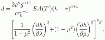
where H is the ice thickness, h is the surface elevation, r is the vertical direction, ![]() and
and ![]() are the components of the transformed mass flux
are the components of the transformed mass flux ![]() and
and ![]() are the horizontal components of the transformed velocity
are the horizontal components of the transformed velocity ![]() is the transformed vertical velocity, M is the surface mass balance, E is the enhancement factor, ρ is the density of ice, g is the acceleration of gravity,
is the transformed vertical velocity, M is the surface mass balance, E is the enhancement factor, ρ is the density of ice, g is the acceleration of gravity, ![]() is thermal diffusivity and c is the specific heat. The constant n = 3 is the power exponent of Glen's flow law. For the rate factor A(T') the Arrhenius relation, with values given by Paterson (1981) and the homologous temperature T', according to T'= Τ + apg(h — r) with ClausiusClapeyron constant a = 7.42 x 10⁻⁵ Κ (kPa)−1, is used.
is thermal diffusivity and c is the specific heat. The constant n = 3 is the power exponent of Glen's flow law. For the rate factor A(T') the Arrhenius relation, with values given by Paterson (1981) and the homologous temperature T', according to T'= Τ + apg(h — r) with ClausiusClapeyron constant a = 7.42 x 10⁻⁵ Κ (kPa)−1, is used.
The boundary conditions at the surface and at the base are
and

respectively, where Ta is the surface temperature, G is the geothermal heat (G = 42x10 −3mWm−2), b* is the basal shear traction, vb, is the sliding velocity and ![]() is the heat conduction (χ = 2.1 wm −1 Κ−1).
is the heat conduction (χ = 2.1 wm −1 Κ−1).
The transformed horizontal velocity is

where

b is the bottom height and VH(b) is the (transformed) sliding velocity. The vertical velocity is

We use a Weert man-type sliding law (Reference WeertmanWeertman, 1964) with exponents after Calov and Huiler (1996). With this it follows, with the transformation (1)1 for the sliding velocity,

where for the sliding parameter the value cs=2.13 x 10⁻⁷ m2 s kg−1 applies. in the model, sliding applies only if the base is at the melting point, i.e. the homologous basal tem-perature equals zero.
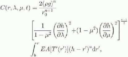
We introduce the diffusivity D as

Comparison with Equations (6), (7) and (9) yields

where

Since sliding only applies if the basal temperature Tb , is at the melting point, the sliding parameter cs in Equation (11) is zero for Tb <0 ("freezing").
Equations (3)-(11) together with the thickness-evolution equation (2) describe the spherical thermomechanical model (CTIM). For the vertically integrated model (CIM) the temperature dependence of the rate factor is ignored ![]() and the sliding parameter cs
is zero everywhere. Thus, temperature evolution in the ice sheet is neglected for the vertically integrated model. For this non-thermomechanical case the integrals in Equation (11) can be solved analytically,
and the sliding parameter cs
is zero everywhere. Thus, temperature evolution in the ice sheet is neglected for the vertically integrated model. For this non-thermomechanical case the integrals in Equation (11) can be solved analytically,

Both ice-sheet models model the reaction of the astheno-sphere to the varying ice load and apply an energy-balance model for the computation of the snow melting al the ice-shect surface.
The model equations are solved on a staggered grid with a stretched σ transformation

In the vertical. The ice-thickness evolution equation is solved semi-implicitly with an allernating-direction-impli-cit scheme. in the temperature-evolution equation vertical derivatives are discretized implicitly, and horizontal derivatives are taken explicitly, with upwind discretisation of the advection term. The horizontal resolution is 0.7° x 0.7° (257 x 256 gridpoints) and the vertical grid spacing is Δζ = 1/15 (16 gridpoints). The model performs different time-steps for the thickness evolution (Δt = 10 years) and the temperature evolution (Δt temp = 100 years).
3. The Coupling of the Ice-Sheet Models and the LLN Climate Model
The LLN model is coupled asynchronously to the vertically integrated CIM or the thermomechanical CTIM. The LLN model includes simplified treatments of the atmosphere, the ocean, the sea ice, the snow-free land and the snowfield. The CIM/CTIM uses the following zonally averaged quantities computed by the LLN model: solar and longwave downward fluxes 500 mb level temperature zonal annual mean precipitation a term representing the contribution of the diurnal and synoptic temperature variance to the sensible-heal flux.
Inversely, the CIM/CTIM provides the LLN model with the spatial extent and mean altitude of the Northern Hemisphere ice sheets.
It is assumed that at the 500 mb level, for all the points situated at the same latitude, the atmosphere is identical to the zonal mean computed by the LLN model. Local radiative fluxes and temperature at the top of the boundary layer are then interpolated from the zonal means, including local characteristics such as altitude. Details of the interpolation process are given in Marsiat (1994).
The LLN model is calculated to steady state, which is reached after 15 years. The zonally averaged climate quantities are input of CIM/CTIM and interpolated to the latitude-longitude grid of CIM/CTIM. After that, CIM or CTIM calculates the change of ice cover over 1000 years. This new ice cover is provided to the LLN model for calculation of a new steady state defining the forcing for the next 1000 years integration of CIM/CTIM. A detailed description of the LLN model can be found in Reference Gallée, van Ypersele, Fichefet, Tricot and BergerGallée and others (1991); for the coupling between the LLN model and CIM sec Marsiat (1994).
4. The Glaciol-Interglaciol Cycle of the Northern Hemisphere
We first introduce two runs with the CIM coupled to the LLN climate model. Run 1 repeats a paleoclimatic simulation of Marsiat (1994) (for the vertically integrated temperature-independent simulation, see Equation (12)) with a

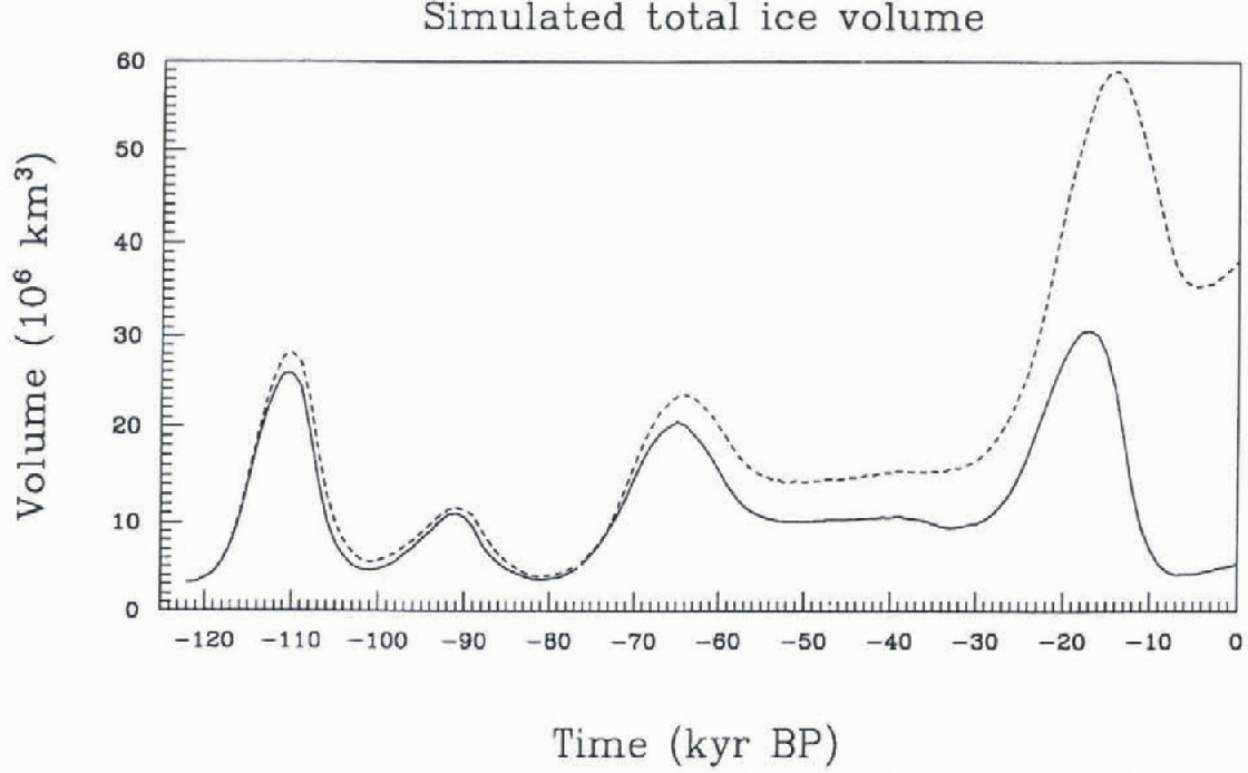
Fig. 1. Total ice volume of the Northern Hemispherefor run 1 (full line) and run 2 (short dashed line). The computations were performed with the vertically integrated ice-sheet model (CIM) using various enhancement factors for the different ice sheets according to Equation (14) (run 1), and a common enhancement factor E =1 for all ice sheets (run 2).

Fig. 2. Shading patlerns of the ice thickness of the Northern Hemisphere in meters, showing snapshots of the simulated Glaciol-interglaciol cycle at the LGM (a) and at present (b) for run 1.
rate factor A = 3 x 10 −16 a−1 Pa −3 and an ice density ρ = 886 kg m−3. For the enhancement factor,

is chosen. For run 2 the enhancement factor E = 1 is used for the whole Northern Hemisphere, while the remaining set-up is as for run 1. CIM/LLN models are integrated (asynchronously) for 122 000 years.
Figure 1 compares the temporal development of the simulated total ice volume of the Northern Hemisphere for runs 1 and 2. The total ice volume of run 1 corresponds well with observations (see Marsiat, 1994). While the difference between the total ice volume of runs 2 and 1 is relatively small in the time-span from 122 to 65 ka BP, it increases considerably after 65 ka BP. At the modelled LGM (17 ka BP) the total ice volume of run 2 is more than twice that of run 1. The simulated present-day ice volume of run 2 differs greatly from observations.
Figure 2 displays the simulated ice thickness at 17 ka BP and the present for run 1. At 17 ka BP (fig. 2a), there are large ice sheets in North America and Eurasia; the whole Tibetan Plateau is glaciated; the ice margin of the Laurentide ice sheet does not extend far enough south; and there is extended glaciation in Siberia, contrary to the findings of CLIMAP (1981), although a smaller Siberian glaciation was found by Reference Tushingham and PeltierTushingham and Peltier (1991). Today's simulated ice thickness (fig. 2b) corresponds relatively well with observations. The great ice sheets have disappeared, though there is still some land ice left. The survival of the Greenland ice sheet corresponds to reality, but the modelled present glaciation of the whole Tibetan Plateau is obviously false. The minor present glaciation of the Rocky Mountains and of north Scandinavia is nearly sub-grid scale. When judging these results one must remember that the whole last Glaciol cycle with minor tuning is modelled in this approach. The build-up and decay of the Northern Hemisphere's land ice is discussed in detail by Marsiat (1994). The reason for the overall minor misfit to observations could be the zonally averaged climate model.
The strong sensitivity of CIM and the LLN model to the enhancement factor is illustrated dramatically by the ice

Fig. 3. As in Figure 2, but for run 2.
thickness from run 2 (see Fig. 3). At the modelled LGM (17kaBP; fig. 3a) the glaciated area of North America and Eurasia is more extended than for run 1 (fig. 2a). The ice thickness of the Eurasian ice sheet increases by 500 m. At the present time the simulated Eurasian ice sheet (fig. 3b) is still there, and its ice is even thicker than at 17 ka BP. A possible explanation of this behaviour is as follows: The lowering of the enhancement factor leads to enlarged ice thickness, because the flow of ice is hampered. The thicker ice has an enlarged accumulation area, because the surface

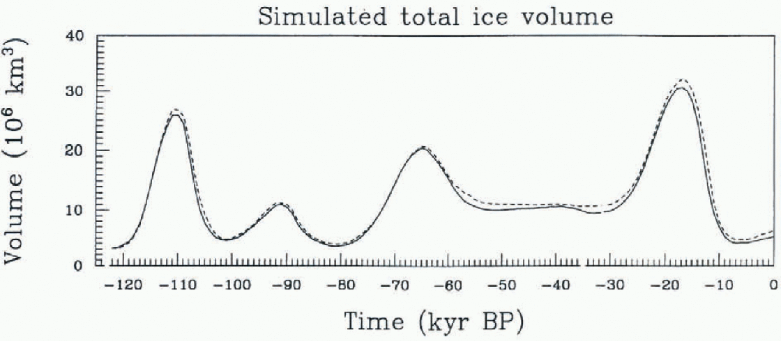
Fig. 4. Fig. 4. Total ice volume of the Northern Hemispherefor the Glaciol—interglaciol cycle, computed with the vertically integrated ice-sheet model (run 3, full line) and the thermomechanical ice-sheet model (run 4, short dashed line).

Fig. 5. Shading patterns of the ice thickness of the Northern Hemisphere in meters, showing snapshots of the simulated Glaciol-interglaciol cycle at the LGM (a) and at present (b) for run 3. Computations were performed with the vertically integrated ice-sheet model (CIM).
slope at the ice margins is steeper than for thinned ice. For thicker ice there is a larger part of the surface which reaches higher and thus colder parts of the atmosphere. There is an increase of ice area for thicker ice, as can be seen by comparing Figures 2a and 3a. Why can thicker ice now spread over the continent? (Before, I wrote that the lowered enhancement factor hampers the flow.) The thicker ice (and the steeper surface slope) must increase the ice velocities to enable more spreading. in addition, large ice area leads to higher planetary albedo and colder climate. Thus a positive feedback contributes to enlarged ice thickness. During the Holocene, when a warmer climate prevails, the thicker ice takes longer to melt if the same melting rate is assumed. These runs demonstrate the importance of the interaction of ice dynamics and climate.
We now compare the vertically integrated ice-sheet model (CIM) with the thermomechanical one (CTIM). For the computation with CIM and the LLN model (run 3) a model set-up as for run 1 is chosen, but with a rate factor A = 2.769 X 10 −16 a−1 Pa −3 and an ice density ρ = 910 kg m−3.
For the thermomechanical simulation with CTIM and the LLN model (run 4) the rate factor A(T') is now temperature-dependent, and Equations (2)-(11) apply. The density is as for run 3, and the enhancement factor is E = 3. Figure 4 compares the simulated total ice volume of runs 3 and 4. Overall, there are only minor differences in the temporal development of ice volume. Run 4 yields about 2 x 10⁶ km3 more ice at the LGM, and at the present there is an increase of approximately 1 x 10⁶ km3 for run 4 compared with run 3. Let us now compare the Northern Hemisphere ice-thickness distribution of run 3 (Fig. 5) and run 4 (Fig. 6) at 17 and 0 ka BP. The ice-covered area is roughly the same for both runs both at 17 ka BP and today, but there are differences in the ice-thickness distribution. At the LGM the Cordilleran and Laurentide ice sheets are thicker for run 4 than for run 3 (see the black shading patterns of the Cordilleran and the 1000-1500 m shading patterns of the Laurentide ice sheet). The thickness patterns of the Eurasian ice sheet show marked differences, the pattern for run 4 being relatively irregular. For both runs 3 and 4, there is a nearly continuous

Fig. 6. As in Figure 5, but using the thermomechanical ice-sheet model (CTIM) for the Glaciol-interglaciol simulation.
Siberian ice sheet. The Scandinavian ice sheet is clearly separated from the Eurasian ice sheet for run 4 but not for run 3. The maximum thickness of the Scandinavian and Siberian ice sheets for run 4 is larger than for run 3, but at 65° N, 90° wthe elevation of the dome of run 3 is the larger. The thickness patterns of the Greenland ice sheet for runs 3 and 4 are also different: the maximum thickness dome of run 4 lies farther north.
The present-day ice-thickness distribution of run 3 (fig. 5b) and run 4 fig. 6b) is now discussed. The 2000-2500 m thickness pattern of the Greenland ice sheet is more extended for run 3 than for run 4, due to sliding in the western part of the Greenland ice sheet caused by the temperate basal area in this region. in the northeast, the ice-thickness gradient of run 4 is steeper than that of run 3; here the cold basal ice hampers the ice flow. Both runs simulate a Tibetan ice sheet at the present day, which is unrealistiC. Clearly, the model is unable to warm up the Tibetan Plateau once it is covered by ice or snow.
Conclusions
We showed that the choice of enhancement factor is crucial for the temporal development of the Northern Hemisphere ice cover if the response of the climate system is treated with the LLN model. We also showed that there are model setups leading to approximately the same ice cover through time for the vertically integrated and for the thermomechanical model. The thermomechanical model contains additional parameters (e.g. the geothermal heat and the sliding coefficient), which are poorly known and can be used to improve the modelling of ice cover through time in detail. Our computations show that the surface mass balance is an important factor in the simulation of the main features of ice cover through the last Glaciol-interglaciol cycle. The discre-pancies (e.g. too much ice in Siberia and too little in North America) can probably be avoided by forcing with a more realistic and geographically explicit climate model. On the other hand, the reaction of the cryosphere/climate system with the enhancement factor is so strong that the thermo-mechanics of ice could also have an important influence, because the ice flow depends on the temperature-dependent rate factor as well as on the enhancement factor.
Outlook
To determine whether the thermomechanical model has essential advantages for paleoclimatic simulations, additional computations need to be carried out (e.g. sensitivity runs with varying geothermal heat and sliding parameter). These will elucidate the question flow sophisticated the ice-sheet model should be for paleo runs and whether a proper representation ofsurface mass balance through time with a climate model is sufficient.
Acknowledgements
We would like to thank A. Berger for the opportunity to work in Louvain-la-Neuve, J.-F. Foccroule for supporting our work with the plot software, R. Greve for help and discussions, and K. Hinter for permission to use the additional computer power of the Institute of Mechanics, Darmstadt, Germany.


