


If I dared, I would say we must have a theory – the word “theory” is so much disliked by so many Englishmen, and is considered by them so “unpractical”, that I avoid it all I can; though I cannot see, myself, that it is very “practical” to do things without knowing the theory of how to do them.
Wintringham & Blashford-Snell (Reference Wintringham and Blashford-Snell1973)1. Introduction
1.1. In Search of a Continuous-time Model of Mortality
Richards & Macdonald (Reference Richards and Macdonald2025) set out some practical benefits of using “continuous-time” models of mortality. This expository paper asks what we mean by a “continuous-time” model of mortality. As we seek an answer, in the theoretical basis of actuarial mortality modelling, we provide the language and notation to keep actuaries abreast of some fairly recent developments. The purpose of the paper is not to provide novel results, but to demonstrate how an actuary can see familiar objects in novel ways.
In fact, the idea of a “continuous-time” model of mortality is not clear-cut or self-contained, and it leads us to consider two contrasts, which we may think of as modelling phenomena on a “micro” scale versus phenomena on a “macro” scale. These are:
-
(a) very informally, the choice of infinitesimal time unit $dx$
versus a discrete time unit, which we take to be a year; and
$dx$
versus a discrete time unit, which we take to be a year; and -
(b) models based on individual lives versus models based on collectives of lives, including, inter alia, the collection of data based on individual lives versus collection of age-grouped data.

1.2. Inspiration from the Life Table
The life table is an obvious source of inspiration. Indeed, in the past some have viewed the whole subject as being the construction of life tables, see for example Batten (Reference Batten1978). A life table is a model of a cohort of identical and independent individuals, followed from some initial selection event at integer age ${x_0} \ge 0$
(such as birth, with
${x_0} \ge 0$
(such as birth, with ${x_0} = 0$
) until mortality has extinguished the whole cohort. It is typically represented by the function
${x_0} = 0$
) until mortality has extinguished the whole cohort. It is typically represented by the function ${l_x}$
, interpreted as the expected number left alive at integer ages
${l_x}$
, interpreted as the expected number left alive at integer ages $x \ge {x_0}$
. The two key features are:
$x \ge {x_0}$
. The two key features are:
-
(a) the focus on the collective rather than the individual; and
-
(b) the time unit of a year
which are both “macro” properties. If we model the number of deaths between integer ages $x$
and
$x$
and $x + 1$
as a random variable
$x + 1$
as a random variable ${D_x}$
, then this formulation of the life table immediately suggests the binomial distribution as a model for
${D_x}$
, then this formulation of the life table immediately suggests the binomial distribution as a model for ${D_x}$
, see Section 2.3.
${D_x}$
, see Section 2.3.
A slightly different view of the life table inspires a different model. Allow ${l_x}$
to range over all real
${l_x}$
to range over all real $x \ge {x_0}$
, not just integer ages, and interpret the ratio
$x \ge {x_0}$
, not just integer ages, and interpret the ratio ${l_{x + n}}/{l_x}$
as the probability that an individual alive at age
${l_{x + n}}/{l_x}$
as the probability that an individual alive at age $x$
survives to age
$x$
survives to age $x + n$
(
$x + n$
( $x \ge {x_0},n \ge 0$
). This leads to further ideas, namely:
$x \ge {x_0},n \ge 0$
). This leads to further ideas, namely:
-
(a) a model in which death is possible at any moment of time; and
-
(b) the force of mortality or hazard rate (our preferred term)
${\mu _x}$
at age
$x$
as a measure of the instantaneous risk of death;


which are both “micro” properties. However, observation is still “macro,” of the collective rather than of the individual. This setup suggests a Poisson model for ${D_x}$
, see Section 2.4.
${D_x}$
, see Section 2.4.
1.3. Models Based on Individuals: The Pseudo-Poisson Model
More recent introductions to the subject begin with the definition of the future lifetime of a person age $x$
as a non-negative random variable, denoted by
$x$
as a non-negative random variable, denoted by ${T_x}$
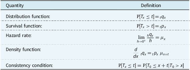
. For brevity and completeness, we compress the definitions of related quantities into Table 1, see Dickson et al. (Reference Dickson, Hardy and Waters2020) or Macdonald et al. (Reference Macdonald, Richards and Currie2018) for details. Of course, the actuarial symbols
${T_x}$
. For brevity and completeness, we compress the definitions of related quantities into Table 1, see Dickson et al. (Reference Dickson, Hardy and Waters2020) or Macdonald et al. (Reference Macdonald, Richards and Currie2018) for details. Of course, the actuarial symbols ${{\rm{\;}}_t}{q_x}{, {}_t}{p_x}$
and
${{\rm{\;}}_t}{q_x}{, {}_t}{p_x}$
and ${\mu _x}$
would be defined, based on the life table, in the process of obtaining the binomial and Poisson models in Section 1.2, but the point is that they are now defined by their rôles in the distribution of
${\mu _x}$
would be defined, based on the life table, in the process of obtaining the binomial and Poisson models in Section 1.2, but the point is that they are now defined by their rôles in the distribution of ${T_x}$
.
${T_x}$
.
Table 1. Definitions of quantities based on ${T_x}$
, the random future lifetime at age
${T_x}$
, the random future lifetime at age $x$
. The consistency condition assumes that
$x$
. The consistency condition assumes that ${x_0} = 0$
, and ensures that calculations based on the distribution of
${x_0} = 0$
, and ensures that calculations based on the distribution of ${T_x}$
will never contradict calculations based on the distribution of
${T_x}$
will never contradict calculations based on the distribution of ${T_y}$
(
${T_y}$
( $y \ne x$
)
$y \ne x$
)
If we define $T_0^i$
to be the random lifetime of the
$T_0^i$
to be the random lifetime of the $i$
th individual under observation, this model focuses attention on:
$i$
th individual under observation, this model focuses attention on:
-
(a) the individual rather than the collective; and
-
(b) events happening instantaneously, meaning during a short time period
$h$
as we let
$h \to {0^ + }$
;


which are both “micro” properties. The most important idea is expressed in the heuristic:
 $${\rm{P}}[{\rm{Dead}}\;{\rm{by}}\;{\rm{age}}\;x + h\;|\,{\rm{Alive}}\;{\rm{at}}\;{\rm{age}}\;x]{ \,= \, _h}{q_x} \approx h\;{\mu _x}\,\,({\rm{for}}\;{\rm{small}}\;h).$$
Knowing the density function of each $T_x^i$
(Table 1), we can write down the probability of any observations, hence a likelihood, and that leads to the following explanation of why the Poisson model of Section 2.4 works so well. Suppose we assume a constant hazard rate at each age, we observe
$T_x^i$
(Table 1), we can write down the probability of any observations, hence a likelihood, and that leads to the following explanation of why the Poisson model of Section 2.4 works so well. Suppose we assume a constant hazard rate at each age, we observe $M$
individuals and there are
$M$
individuals and there are $D$
deaths. Then:
$D$
deaths. Then:
-
(a) the model based on individual random lifetimes gives us, correctly, non-zero probabilities only of observing
$0,1, \ldots, M$
deaths, while -
(b) a Poisson distribution would give us, incorrectly, non-zero probabilities also of observing
$M + 1,M + 2, \ldots $
deaths.


Moreover, unless the total time exposed-to-risk is a deterministic constant, fixed in advance by the observational scheme, the number of deaths cannot be Poisson (Macdonald, Reference Macdonald1996). However, both models above have the same likelihood, as if they were Poisson. It follows that likelihood-based inference will be identical under either model. This leads us to call the model based on age-grouped data (and a constant hazard) the pseudo-Poisson model (Section 3.7). We continue to seek the proper foundations of a mortality model at the “micro” level in the model of individual lifetimes.
1.4. Dynamic Life History Models I: Truncation and Censoring
The individual life history model lets us write down exact probabilities of observed events, if we know the hazard rates. It also lets us deal with incomplete observation, in particular:
-
(a) left-truncation: an individual enters observation having already survived to some age
${x_a} \gt 0$
; and -
(b) right-censoring: the individual leaves observation while still alive, so we observe only that
${T_{{x_a}}} \gt {x_b - x_a}$
for some age
${x_b} \gt {x_a}$
.


A neat device allows us to avoid the complication of keeping track of ages ${x_a}$
and
${x_a}$
and ${x_b}$
when writing expressions such as likelihoods. Define a process:
${x_b}$
when writing expressions such as likelihoods. Define a process:
 $${Y^i}\left( x \right) = {I_{\left\{ {i{\rm{th\;individual\;alive\;and\;under\;observation\;at\;age\;}}{x^ - }} \right\}}}$$
(age ${x^ - }$
means “just before age
${x^ - }$
means “just before age $x$
” and is a technicality). The “under observation” condition takes care of left-truncation and right-censoring. Then, for example, the integrated hazard rate over the time spent under observation by the
$x$
” and is a technicality). The “under observation” condition takes care of left-truncation and right-censoring. Then, for example, the integrated hazard rate over the time spent under observation by the $i$
th individual (an important quantity in many calculations), can be written:
$i$
th individual (an important quantity in many calculations), can be written:
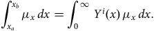 $$\mathop \int \nolimits_{{x_a}}^{{x_b}} {\mu _x}{\rm{\,}}dx = \mathop \int \nolimits_0^\infty {Y^i}\left( x \right){\rm{\,}}{\mu _x}{\rm{\,}}dx.$$
We see that the process ${Y^i}\left( x \right){\rm{\;}}{\mu _x}$
acts as a dynamic or stochastic hazard rate tailored to the
${Y^i}\left( x \right){\rm{\;}}{\mu _x}$
acts as a dynamic or stochastic hazard rate tailored to the $i$
th individual, and greatly simplifies expressions involving integrals, since all integrals can now be now taken over
$i$
th individual, and greatly simplifies expressions involving integrals, since all integrals can now be now taken over $\left( {0,\infty } \right]$
(Section 4.6).
$\left( {0,\infty } \right]$
(Section 4.6).
1.5. Dynamic Life History Models II: Back to Bernoulli
In a utilitarian sense the job was finished with Section 1.3, but the heuristic (1) suggests more to come. For, if ${{\rm{\;}}_h}{q_x} \approx h{\rm{\,}}{\mu _x}$
then
${{\rm{\;}}_h}{q_x} \approx h{\rm{\,}}{\mu _x}$
then ${{\rm{\;}}_h}{p_x} \approx 1 - h{\rm{\,}}{\mu _x}$
, and if we let
${{\rm{\;}}_h}{p_x} \approx 1 - h{\rm{\,}}{\mu _x}$
, and if we let ${\delta _x}$
be an indicator, equal to 1 if death occurs at age
${\delta _x}$
be an indicator, equal to 1 if death occurs at age $x$
, and 0 otherwise, then what is observed “during” time
$x$
, and 0 otherwise, then what is observed “during” time $h$
is the outcome of a Bernoulli trial with parameter
$h$
is the outcome of a Bernoulli trial with parameter $h{\rm{\,}}{\mu _x}$
and probability:
$h{\rm{\,}}{\mu _x}$
and probability:
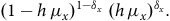 $${(1 - h{\rm{\,}}{\mu _x})^{1 - {\delta _x}}}{\rm{\;}}{(h{\rm{\,}}{\mu _x})^{{\delta _x}}}.$$
We would like to take all such consecutive “instantaneous” Bernoulli trials while the individual is alive and under observation, and multiply their probabilities (4) together. In all of probability theory, there is nothing simpler than a Bernoulli trial, so we really would have reduced a probability in a mortality model to its constituent “atoms”; the ultimate “micro” level. That is what we describe in Section 4. To do so we introduce two ideas, which give us the notation needed to write down a product of Bernoulli probabilities like (4) in a rigorous way.
-
(a) Counting processes: A counting process
${N^i}\left( x \right)$
starts at
${N^i}\left( 0 \right) = 0$
and jumps to 1 at time
$T_0^i$
if the
$i$
th individual is then under observation. Then its increment
$d{N^i}\left( x \right)$
indicates an observed death, and is a rigorous version of the informal
${\delta _x}$
in (4). Between them,
${N^i}\left( x \right)$
and
${Y^i}\left( x \right)$
let us write the Bernoulli trial probability (4) formally as:


 $${(1 - {Y^i}\left( x \right){\rm{\,}}{\mu _x}{\rm{\,}}dx)^{1 - d{N^i}\left( x \right)}}{\rm{\;}}{({Y^i}\left( x \right){\rm{\,}}{\mu _x}{\rm{\,}}dx)^{d{N^i}\left( x \right)}}$$
and this allows for left-truncation and right-censoring.
-
(b) Product-integral: The product-integral is the device that lets us multiply all the infinitesimal Bernoulli trial probabilities. We defer further description to Section 4.2 and Appendix B and just give the final form of the likelihood contributed by the
$i$
th individual, denoted by
${L_i}$
:


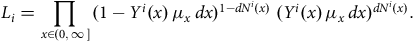 $${L_i} = \mathop \prod \limits_{x \in \left( {0,\infty } \right]} {(1 - {Y^i}\left( x \right){\rm{\,}}{\mu _x}{\rm{\,}}dx)^{1 - d{N^i}\left( x \right)}}{\rm{\;}}{({Y^i}\left( x \right){\rm{\,}}{\mu _x}{\rm{\,}}dx)^{d{N^i}\left( x \right)}}.$$
The product-integral is identified by a product over all values of an interval ( $x \in \left( {0,\infty } \right]$
here) and the presence of the variable of integration (
$x \in \left( {0,\infty } \right]$
here) and the presence of the variable of integration ( $dx$
here) in the integrand.
$dx$
here) in the integrand.
1.6. What is a “Continuous-time” Model?
We started out by trying to pin down what we meant by the vague term “continuous-time mortality model.” Our answer is: it is the class of models with Poisson-like likelihoods built up, by product integration, out of infinitesimal Bernoulli trials (see Section 4.8 and Figure 2). Any model in this class has the following properties.
-
(a) It is irreducible, in the sense that it is composed of (infinitesimal) Bernoulli trials.
-
(b) It is based on behaviour at the “micro” time scale.
-
(c) It is based on individual lives.
-
(d) Aggregated, over time and over individuals, it explains the Poisson-like nature of likelihoods, therefore estimation based on the collective at the “macro” time scale.
-
(e) It allows for left-truncation and right-censoring.
-
(f) It is easily extended to multiple-decrement and multiple-state models.
This class includes, as a special case, true Poisson distributions, but these are always associated with an improbable observational plan. Note that our endpoint is just the starting point for the modern statistical study of survival models (Section 4.10), see Andersen et al. (Reference Andersen, Borgan, Gill and Keiding1993).
1.7. Plan of this Paper
We start in Section 2 with Forfar et al. (Reference Forfar, McCutcheon and Wilkie1988), a definitive account of graduation using binomial and Poisson models, which we call mortality models at the “macro” scale. Then in Section 3 we turn to models at the “micro” scale based on individual lifetimes, and find the origins of Poisson-like behaviour at the “macro” scale. In Section 4 we bring together models of individual lifetimes and models based on behaviour over small intervals $h$
as
$h$
as $h \to {0^ + }$
, and find that all probabilities in a mortality model arise as a product of consecutive (infinitesimal) Bernoulli trials. Section 5 concludes.
$h \to {0^ + }$
, and find that all probabilities in a mortality model arise as a product of consecutive (infinitesimal) Bernoulli trials. Section 5 concludes.
2. Binomial and Poisson Models
2.1. Forfar et al. (Reference Forfar, McCutcheon and Wilkie1988)
In a landmark paper, Forfar et al. (Reference Forfar, McCutcheon and Wilkie1988) gave comprehensive accounts of two models for survival data, namely the binomial and Poisson models. These defined: (a) the random variable ${D_x}$
, to be the number of deaths observed at age
${D_x}$
, to be the number of deaths observed at age $x$
; and (b) a suitable measure of exposure to risk at age
$x$
; and (b) a suitable measure of exposure to risk at age $x$
, assumed to be non-random, that we will call
$x$
, assumed to be non-random, that we will call ${V_x}$
. Then the occurrence-exposure rate
${V_x}$
. Then the occurrence-exposure rate ${D_x}/{V_x}$
was shown to be an estimate of the model parameter, a mortality rate
${D_x}/{V_x}$
was shown to be an estimate of the model parameter, a mortality rate $\hat q$
in the binomial model, and a hazard rate
$\hat q$
in the binomial model, and a hazard rate $\hat \mu $
in the Poisson modelFootnote
1
.
$\hat \mu $
in the Poisson modelFootnote
1
.
Forfar et al. (Reference Forfar, McCutcheon and Wilkie1988) helpfully located the old subject of parametric graduation in a modern statistical setting, including model specification, likelihood, score function and information, covariance matrix, model selection and parametric bootstrapping. The treatment was heavily influenced by the authors’ work for the Continuous Mortality Investigation Bureau (the CMIB, now CMI) particularly in respect of data collection. The advance it represented may be gauged by comparison with contemporary texts such as Batten (Reference Batten1978) and Benjamin and Pollard (Reference Benjamin and Pollard1980).
Both binomial and Poisson models are rooted in simple thought-experiments, require no statistics beyond a first course in data analysis, and can, with qualifications, be implemented in standard statistical packages such as R (R Core Team, 2021). This gives them considerable staying power.
2.2. The Rate Interval and
${{\bf{\Delta }}_k}$
Notation

The rate interval is an interval of age (or calendar time) on which an individual is assigned a given age label. It is the means of assigning an age label to an individual exposed to the risk of death and at the time of death. Note that rate intervals are only needed with age-grouped data, not models based on individual lives. They are treated in detail in texts such as Benjamin and Pollard (Reference Benjamin and Pollard1980). We assume that the rate interval, when we need one, is the year of age $\left( {x,x + 1} \right]$
defined by “age last birthday.” The CMI, for another example, use the year of age
$\left( {x,x + 1} \right]$
defined by “age last birthday.” The CMI, for another example, use the year of age $\left( {x - 1/2,x + 1/2} \right]$
defined by “age nearest birthday.”
$\left( {x - 1/2,x + 1/2} \right]$
defined by “age nearest birthday.”
We assume that the data are covered by $K$
rate intervals and that in the abstract these may be denoted by
$K$
rate intervals and that in the abstract these may be denoted by ${{\rm{\Delta }}_k}$ $\left( {k = 1,2, \ldots, K} \right)$
; and that a sum over all rate intervals may be denoted by
$\left( {k = 1,2, \ldots, K} \right)$
; and that a sum over all rate intervals may be denoted by $\mathop \sum \nolimits_k $
, and a product likewise by
$\mathop \sum \nolimits_k $
, and a product likewise by $\mathop \prod \nolimits_k $
.
$\mathop \prod \nolimits_k $
.
2.3. Binomial Models
The binomial model is based on the following thought-experiment: take ${E_x}$
lives at the start of a year, all alive at age
${E_x}$
lives at the start of a year, all alive at age $x$
and assumed to be “statistically independent” in respect of their mortality risk. Then
$x$
and assumed to be “statistically independent” in respect of their mortality risk. Then ${E_x}$
is the measure of exposure referred to as
${E_x}$
is the measure of exposure referred to as ${V_x}$
in Section 2.1, usually here called the initial exposed-to-risk. Define
${V_x}$
in Section 2.1, usually here called the initial exposed-to-risk. Define ${D_x}$
to be the number who are dead at the end of the year, and
${D_x}$
to be the number who are dead at the end of the year, and ${q_x}$
to be the probability that a life alive at age
${q_x}$
to be the probability that a life alive at age $x$
dies not later than age
$x$
dies not later than age $x + 1$
. Then the following are easily shown.
$x + 1$
. Then the following are easily shown.
-
(a)
${D_x}$
has a
${\rm{\;binomial}}\left( {{E_x},{q_x}} \right)$
distribution, with first two moments
${\rm{\;E\;}}\left[ {{D_x}} \right] = {E_x}{\rm{\;}}{q_x}$
and
${\rm{\;Var\;}}\left[ {{D_x}} \right] = {E_x}{\rm{\;}}{q_x}{\rm{\;}}\left( {1 - {q_x}} \right)$
. -
(b) As a function of parameter
${q_x}$
, the data
$\left( {{D_x},{E_x}} \right)$
has likelihood function:


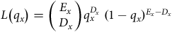 $$L\left( {{q_x}} \right) = \left( {\matrix{{{E_x}} \cr {{D_x}} \cr } } \right)q_x^{{D_x}}\;{(1 - {q_x})^{{E_x} - {D_x}}}$$
 $$ \propto q_x^{{D_x}}{\rm{\;}}{(1 - {q_x})^{{E_x} - {D_x}}},$$
leading to the maximum likelihood estimate (MLE) ${\hat q_x} = {D_x}/{E_x}$
which is asymptotically unbiased (
${\hat q_x} = {D_x}/{E_x}$
which is asymptotically unbiased ( ${\rm{E}}\left[ {{{\hat q}_x}} \right] = {q_x}$
) with variance
${\rm{E}}\left[ {{{\hat q}_x}} \right] = {q_x}$
) with variance ${\rm{\;Var\;}}\left[ {{{\hat q}_x}} \right] = {q_x}{\rm{}}\left( {1 - {q_x}} \right)/{E_x}$
.
${\rm{\;Var\;}}\left[ {{{\hat q}_x}} \right] = {q_x}{\rm{}}\left( {1 - {q_x}} \right)/{E_x}$
.
-
(c) The estimate
${\hat q_x}$
is an estimate of
${q_x}$
, that is, the function value at start of the rate interval
$\left( {x,x + 1} \right]$
.


 ${D_x}$
can be viewed as the number of successes out of
${D_x}$
can be viewed as the number of successes out of ${E_x}$
independent Bernoulli trials, each with probability of success (death) equal to
${E_x}$
independent Bernoulli trials, each with probability of success (death) equal to ${q_x}$
. The idea of the Bernoulli trial as the fundamental “atom” of mortality risk appears again in Section 4.5.
${q_x}$
. The idea of the Bernoulli trial as the fundamental “atom” of mortality risk appears again in Section 4.5.
2.4. Poisson Models
The Poisson model depends on a different thought-experiment. An unspecified number of individuals is observed, alive during the relevant rate interval of age $\left( {x,x + 1} \right]$
, such that the total time alive and under observation is a non-random quantity
$\left( {x,x + 1} \right]$
, such that the total time alive and under observation is a non-random quantity $E_x^c$
. Now
$E_x^c$
. Now $E_x^c$
is the measure of exposure referred to as
$E_x^c$
is the measure of exposure referred to as ${V_x}$
in Section 2.1, usually here called the central exposed-to-risk. A constant force of mortality
${V_x}$
in Section 2.1, usually here called the central exposed-to-risk. A constant force of mortality $\mu $
is assumed at all ages in the rate interval
$\mu $
is assumed at all ages in the rate interval $\left( {x,x + 1} \right]$
. Define
$\left( {x,x + 1} \right]$
. Define ${D_x}$
to be the number of observed deaths. Then the following can be shown.
${D_x}$
to be the number of observed deaths. Then the following can be shown.
-
(a)
${D_x}$
has a
${\rm{\;Poisson}}\left( {\mu {\rm{\,}}E_x^c} \right)$
distribution with first two moments
${\rm{E}}\left[ {{D_x}\left] { = {\rm{Var}}} \right[{D_x}} \right] = \mu {\rm{\,}}E_x^c$
. -
(b) As a function of parameter
$\mu $
, the data
$\left( {{D_x},E_x^c} \right)$
has likelihood function:
$$L\left( \mu \right) = {(\mu {\rm{\,}}E_x^c)^{{D_x}}}{\rm{\;exp}}\left( { - \mu {\rm{\,}}E_x^c} \right)/{D_x}!$$
(8)
$${\propto {\rm{exp}}\left( { - \mu {\rm{\,}}E_x^c} \right){\rm{\;}}{\mu ^{{D_x}}},}$$
leading to the MLE
$\hat \mu = {D_x}/E_x^c$
which is asymptotically unbiased (
${\rm{E\;}}\left[ {\hat \mu } \right] = {\mu _x}$
) with variance
${\rm{Var}}\left[ {\hat \mu } \right] = \mu /E_x^c$
. -
(c) Assuming a relatively even distribution of exposure over the rate interval
$\left( {x,x + 1} \right]$
, the MLE
$\hat \mu $
estimates
${\mu _{x + 1/2}}$
.


2.5. Terminology
Binomial and Poisson models may be described in different ways. The binomial model admits of no conceivable time other than its own time unit; it is unambiguously a discrete-time model. It may also be called a $q$
-type model in honour of its conventional parameter. The Poisson model is a candidate for a continuous-time model, although it turns out to be an extreme representative of a whole class, see Sections 3 et seq. It may also be called a
$q$
-type model in honour of its conventional parameter. The Poisson model is a candidate for a continuous-time model, although it turns out to be an extreme representative of a whole class, see Sections 3 et seq. It may also be called a $\mu $
-type model in honour of its conventional parameter. See Richards and Macdonald (Reference Richards and Macdonald2025) for both terminologies.
$\mu $
-type model in honour of its conventional parameter. See Richards and Macdonald (Reference Richards and Macdonald2025) for both terminologies.
2.6. Assessment of the Binomial and Poisson Models
2.6.1. Feasibility of the Thought-Experiment: Binomial Model
To carry out the binomial thought-experiment we would need a homogeneous sample of ${E_x}$
individuals age
${E_x}$
individuals age $x$
, observed to be alive or dead at age
$x$
, observed to be alive or dead at age $x + 1$
. This contrasts with observation of (say) members of a pension scheme or life office policyholders. Real data often includes exits for reasons other than death and not under the modeller’s control, see Richards and Macdonald (Reference Richards and Macdonald2025), Section 3 and Appendix for examples. The requirements of the binomial experiment will not be met by: (a) individuals entering observation between ages
$x + 1$
. This contrasts with observation of (say) members of a pension scheme or life office policyholders. Real data often includes exits for reasons other than death and not under the modeller’s control, see Richards and Macdonald (Reference Richards and Macdonald2025), Section 3 and Appendix for examples. The requirements of the binomial experiment will not be met by: (a) individuals entering observation between ages $x$
and
$x$
and $x + 1$
; and (b) individuals leaving observation between ages
$x + 1$
; and (b) individuals leaving observation between ages $x$
and
$x$
and $x + 1$
, for reasons other than death.
$x + 1$
, for reasons other than death.
Thus we are led to ask, what is the probability of surviving over any fraction of the rate interval? For example, an individual joining at age $x - 1/2$
and surviving to age
$x - 1/2$
and surviving to age $x$
requires the calculation of
$x$
requires the calculation of ${{\rm{\;}}_{1/2}}{p_{x - 1/2}}$
. The binomial model gives no satisfactory answer. Strictly, the question lies outside the bounds of the model. Even if we could implement the thought-experiment, the model posits only the number of lives observed at the start and end of the rate interval.
${{\rm{\;}}_{1/2}}{p_{x - 1/2}}$
. The binomial model gives no satisfactory answer. Strictly, the question lies outside the bounds of the model. Even if we could implement the thought-experiment, the model posits only the number of lives observed at the start and end of the rate interval.
Nevertheless, an answer may be demanded, because individuals can and do join or leave an investigation in the middle of the rate interval, see (Richards and Macdonald, Reference Richards and Macdonald2025, Section 3) for numerous examples in practice. The analyst is obliged to make some assumption about mortality between ages $x$
and
$x$
and $x + 1$
, for which the binomial model gives no guidance. Three popular assumptions have been:
$x + 1$
, for which the binomial model gives no guidance. Three popular assumptions have been:
-
(a) a uniform distribution of deaths;
-
(b) the Balducci hypothesis; and
-
(c) a constant hazard rate.
See Macdonald (Reference Macdonald1996) or Richards and Macdonald (Reference Richards and Macdonald2025) for a discussion of these. Here we just remark that (c), a constant hazard rate, is mathematically the simplest, fully consistent with the Poisson model, and also consistent with modelling individual lifetimes as in Section 3.
2.6.2. Feasibility of the Thought-Experiment: Poisson Model
The Poisson thought-experiment is not troubled by fractions of the rate interval. Since the hazard rate is assumed to be a constant $\mu $
during the rate interval
$\mu $
during the rate interval $\left( {x,x + 1} \right]$
, the probability of dying during the sub-interval
$\left( {x,x + 1} \right]$
, the probability of dying during the sub-interval $\left( {x + a,x + b} \right]$
(given alive at age
$\left( {x + a,x + b} \right]$
(given alive at age $x + a$
, for
$x + a$
, for $0 \le a \lt b \le 1$
) is
$0 \le a \lt b \le 1$
) is $1 - {\rm{exp}}\left( { - \mu {\rm{\,}}\left( {b - a} \right)} \right)$
.
$1 - {\rm{exp}}\left( { - \mu {\rm{\,}}\left( {b - a} \right)} \right)$
.
The Poisson thought-experiment is not met in practice, however, for different reasons. The distribution of ${D_x}$
is Poisson only if the exposed-to-risk
${D_x}$
is Poisson only if the exposed-to-risk $E_x^c$
is non-random, for example pre-determined. This is not the case if: (a) the population being sampled is finite, with known maximum size
$E_x^c$
is non-random, for example pre-determined. This is not the case if: (a) the population being sampled is finite, with known maximum size $M$
individuals, say, because then
$M$
individuals, say, because then ${D_x} \le M$
, but
${D_x} \le M$
, but ${\rm{\;P\;}}[{D_x} \gt M] \gt 0$
under any Poisson distribution; or (b) the exposure times of the individuals in the sampled population are not known in advance, because then
${\rm{\;P\;}}[{D_x} \gt M] \gt 0$
under any Poisson distribution; or (b) the exposure times of the individuals in the sampled population are not known in advance, because then $E_x^c$
is random. Moreover,
$E_x^c$
is random. Moreover, ${D_x}$
is usually a component of the bivariate random variable
${D_x}$
is usually a component of the bivariate random variable $\left( {{D_x},E_x^c} \right)$
. In such cases we call
$\left( {{D_x},E_x^c} \right)$
. In such cases we call ${D_x}$
pseudo-Poisson, see Section 3. For estimation purposes, however, it behaves as a true Poisson random variable would, see Section 3.7.
${D_x}$
pseudo-Poisson, see Section 3. For estimation purposes, however, it behaves as a true Poisson random variable would, see Section 3.7.
2.6.3. Occurrence-exposure Rates, Age-grouped Data and Graduation
The estimates ${\hat q_x} = {D_x}/{E_x}$
and
${\hat q_x} = {D_x}/{E_x}$
and ${\hat \mu _x} = {D_x}/E_x^c$
are examples of occurrence-exposure rates. Both they and their sample variances (Sections 2.3 and 2.4) require only the age-grouped totals
${\hat \mu _x} = {D_x}/E_x^c$
are examples of occurrence-exposure rates. Both they and their sample variances (Sections 2.3 and 2.4) require only the age-grouped totals ${D_x}$
and
${D_x}$
and ${E_x}$
or
${E_x}$
or $E_x^c$
to be reported to the analyst, rather than data on each individual. Such totals may easily be extracted from ordinary data files used in the business; they greatly reduce the volume of data required (which used to matter a lot); and they reduce the risk of accidentally breaching data-protection rules (which matters now). On the other hand they do not allow the level of checking and cleaning of the data that is possible with individual data (Macdonald et al., Reference Macdonald, Richards and Currie2018, Chapter 2).
$E_x^c$
to be reported to the analyst, rather than data on each individual. Such totals may easily be extracted from ordinary data files used in the business; they greatly reduce the volume of data required (which used to matter a lot); and they reduce the risk of accidentally breaching data-protection rules (which matters now). On the other hand they do not allow the level of checking and cleaning of the data that is possible with individual data (Macdonald et al., Reference Macdonald, Richards and Currie2018, Chapter 2).
If age-grouped data are prepared by someone other than the analyst, the modelling is wholly dependent on the thoroughness and diligence of the source provider. This is a material concern for risk transfer transactions, such as reinsurance, bulk annuities and portfolio transfers. If a model is to be used to price a risk transfer, the analyst should always insist on individual records, regardless of whether the intent is to use models based on individuals or age-grouped counts.
Occurrence-exposure rates ${\hat q_x}$
or
${\hat q_x}$
or ${\hat \mu _x}$
are normally smoothed or graduated for practical use. For this purpose a likelihood may be calculated as the product of the likelihoods for each rate interval, using age-grouped data. Other, non-likelihood methods may also be used (Forfar et al., Reference Forfar, McCutcheon and Wilkie1988).
${\hat \mu _x}$
are normally smoothed or graduated for practical use. For this purpose a likelihood may be calculated as the product of the likelihoods for each rate interval, using age-grouped data. Other, non-likelihood methods may also be used (Forfar et al., Reference Forfar, McCutcheon and Wilkie1988).
2.7. Generalized Linear Models (GLMs)
To the list of properties in Sections 2.3 and 2.4 we could have added “(d) Leads to a simple Generalized Linear Model (GLM) for graduating age-grouped mortality data.”
GLMs were introduced by Nelder and Wedderburn (Reference Nelder and Wedderburn1972), and contain three elements: (a) a random component, ${Y_x}$
; (b) a systematic component,
${Y_x}$
; (b) a systematic component, ${\eta _x}$
; and (c) a link function,
${\eta _x}$
; and (c) a link function, $g$
. A GLM connects the expectation of
$g$
. A GLM connects the expectation of ${Y_x}$
to
${Y_x}$
to ${\eta _x}$
via
${\eta _x}$
via $g$
as follows:
$g$
as follows:
 $${\eta _x} = g\left( {{\rm{E}}\left[ {{Y_x}} \right]} \right).$$
The component ${\eta _x}$
is the linear predictor; in mortality work it is a linear function of age,
${\eta _x}$
is the linear predictor; in mortality work it is a linear function of age, $x$
, and a corresponding covariate vector,
z
$x$
, and a corresponding covariate vector,
z ${{\rm{\;\!}}_x}$
. Let
θ
be the vector of parameters to estimate, and let
X
be the corresponding model matrix. Each observation
${{\rm{\;\!}}_x}$
. Let
θ
be the vector of parameters to estimate, and let
X
be the corresponding model matrix. Each observation ${Y_x}$
has a corresponding row in
X
. For a binomial GLM we have:
${Y_x}$
has a corresponding row in
X
. For a binomial GLM we have:
 $${Y_x} = {{{D_x}} \over {{E_x}}},\;\;\;\;\;\;\;\;{\eta _x} = {\boldsymbol X \theta} \left[ {x,{\rm{\;}}} \right].$$
For a Poisson GLM with the link function $g\left( x \right) = {\rm{log}}\left( x \right)$
we have:
$g\left( x \right) = {\rm{log}}\left( x \right)$
we have:
 $${Y_x} = {D_x},{\rm{\;\;\;\;\;\;\;\;}}{\eta _x} = {\boldsymbol X\theta} \left[ {x,{\rm{\;}}} \right] + {\rm{log}}\left( {E_x^c} \right).$$
where $\left[ {x,{\rm{\;}}} \right]$
selects the row for the observation corresponding to age
$\left[ {x,{\rm{\;}}} \right]$
selects the row for the observation corresponding to age $x$
.
$x$
.
The link function, $g$
, is chosen by the analyst. The canonical link for the binomial GLM is the logit, but other link functions can be used, such as the probit link. The canonical link for the Poisson GLM is the logarithm, but other link functions have been used for mortality work, such as the logit link; see Currie (Reference Currie2016), Appendix A for implementation details of the logit link for Poisson GLMs.
$g$
, is chosen by the analyst. The canonical link for the binomial GLM is the logit, but other link functions can be used, such as the probit link. The canonical link for the Poisson GLM is the logarithm, but other link functions have been used for mortality work, such as the logit link; see Currie (Reference Currie2016), Appendix A for implementation details of the logit link for Poisson GLMs.
GLMs have a link with “classical” actuarial modelling since one of the simplest choices of fitted ${\hat \eta _x}$
is a Gompertz function, but this does not extend to other members of the Gompertz-Makeham family (see Forfar et al. (Reference Forfar, McCutcheon and Wilkie1988)).
${\hat \eta _x}$
is a Gompertz function, but this does not extend to other members of the Gompertz-Makeham family (see Forfar et al. (Reference Forfar, McCutcheon and Wilkie1988)).
GLMs are popular because they are flexible, have nice statistical properties and are linear in the covariates. The binomial and Poisson error structures arise naturally for “count” data, and age-grouped deaths are examples of “counts” so these GLMs are, in a sense, natural candidates as mortality models. However, linear dependence on covariates, and the canonical link functions associated with the exponential family, are restrictive, and for large experiences we will often find better-fitting models that are not GLMs (see, for example, the range of models included in Cairns et al. (Reference Cairns, Blake, Dowd, Coughlan, Epstein, Ong and Balevich2009)). In addition GLMs bring us no closer to any foundational concept of a “mechanism” generating mortality data, so we do not consider them further.
3. Modelling Individual Lifetimes: The Pseudo-Poisson Model
3.1. Observation of an Individual
Suppose the $i$
th individual is observed from age
$i$
th individual is observed from age ${x_i}$
until age
${x_i}$
until age ${y_i}$
for total time
${y_i}$
for total time ${v_i} = {y_i} - {x_i}$
. Denote the interval
${v_i} = {y_i} - {x_i}$
. Denote the interval $\left( {{x_i},{y_i}} \right]$
by
$\left( {{x_i},{y_i}} \right]$
by ${{\rm{\Delta }}_i}$
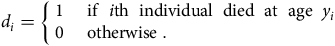
. Observation ends because of either death or right-censoring at age
${{\rm{\Delta }}_i}$
. Observation ends because of either death or right-censoring at age ${y_i}$
. Define the indicator:
${y_i}$
. Define the indicator:
 $${d_i} = \left\{ {\matrix{ 1 \hfill & {{\rm{\;if\;\;}}i{\rm{th\;\;individual\;\;died\;\;at\;\;age\;\;}}{y_i}{\rm{\;}}} \hfill \cr 0 \hfill & {{\rm{\;otherwise\;}}.} \hfill \cr } } \right.$$
Then the random variable observed is the bivariate $\left( {{d_i},{v_i}} \right)$
, and the total contribution to the likelihood of these observations, denoted by
$\left( {{d_i},{v_i}} \right)$
, and the total contribution to the likelihood of these observations, denoted by ${L_i}$
, is:
${L_i}$
, is:
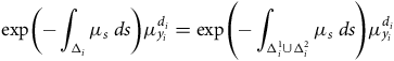
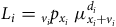 $${L_i}\;{ =\; _{{v_i}}}{p_{{x_i}}}{\rm{\;}}\mu _{{x_i} + {v_i}}^{{d_i}}$$
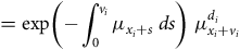 $$ \hskip 76pt= {\rm{exp}}\left( { - \mathop \int \nolimits_0^{{v_i}} {\mu _{{x_i} + s}}{\rm{\;}}ds} \right){\rm{\;}}\mu _{{x_i} + {v_i}}^{{d_i}}$$
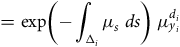 $$ \hskip 54pt= {\rm{exp}}\left( { - \mathop \int \nolimits_{{{\rm{\Delta }}_i}} {\mu _s}{\rm{\;}}ds} \right){\rm{\;}}\mu _{{y_i}}^{{d_i}}$$
see Table 1, or Macdonald et al. (Reference Macdonald, Richards and Currie2018), Chapter 5.
3.2. Age Intervals and
${{\rm{\Delta }}_i}$
Notation

The definition of the interval ${{\rm{\Delta }}_i}$
depends on the observational plan and the method of investigation. The important point is that it is time under observation of a single individual, the
${{\rm{\Delta }}_i}$
depends on the observational plan and the method of investigation. The important point is that it is time under observation of a single individual, the $i$
th of
$i$
th of $M$
individuals. Some examples are the following.
$M$
individuals. Some examples are the following.
-
(a) The interval may be the entire period for which the
$i$
th individual was observed, potentially spanning many years. -
(b) The interval may be that part of a rate interval (for example, year of age) for which the
$i$
th individual was under observation. -
(c) The interval may be an interval of age on which the hazard rate is assumed to be constant.


Therefore the likelihood (13) based on ${{\rm{\Delta }}_i}$
may constitute the whole of the
${{\rm{\Delta }}_i}$
may constitute the whole of the $i$
th individual’s contribution to the total likelihood, or only part of it. We will call a contribution to a likelihood of the form (13) a survival model likelihood, whether it forms all or part of the
$i$
th individual’s contribution to the total likelihood, or only part of it. We will call a contribution to a likelihood of the form (13) a survival model likelihood, whether it forms all or part of the $i$
th individual’s contribution, and whether or not hazard rates are assumed to be piecewise-constant.
$i$
th individual’s contribution, and whether or not hazard rates are assumed to be piecewise-constant.
3.3. Multiplication and Factorization of Survival Model Likelihoods
Survival model likelihoods in respect of the same individual over contiguous intervals, multiplied together, give another survival model likelihood. In reverse, a survival model likelihood may be factorized into as many factors of like kind as we please. To see the multiplicative property, suppose the $i$
th individual is observed on the contiguous intervals
$i$
th individual is observed on the contiguous intervals ${\rm{\Delta }}_i^1 = \left( {{x_i},{z_i}} \right]$
and
${\rm{\Delta }}_i^1 = \left( {{x_i},{z_i}} \right]$
and ${\rm{\Delta }}_i^2 = \left( {{z_i},{y_i}} \right]$
, and that indicators of death
${\rm{\Delta }}_i^2 = \left( {{z_i},{y_i}} \right]$
, and that indicators of death $d_i^{\left( 1 \right)}$
at time
$d_i^{\left( 1 \right)}$
at time ${z_i}$
and
${z_i}$
and $d_i^{\left( 2 \right)}$
at time
$d_i^{\left( 2 \right)}$
at time ${y_i}$
are defined analagously to
${y_i}$
are defined analagously to ${d_i}$
above. Then if
${d_i}$
above. Then if ${{\rm{\Delta }}_i} = \left( {{x_i},{y_i}} \right]$
as before:
${{\rm{\Delta }}_i} = \left( {{x_i},{y_i}} \right]$
as before:
 $$\hskip-100pt{\rm{exp}}\left( { - \mathop \int \nolimits_{{{\rm{\Delta }}_i}} {\mu _s}{\rm{\;}}ds} \right)\mu _{{y_i}}^{{d_i}} = {\rm{exp}}\left( { - \mathop \int \nolimits_{{\rm{\Delta }}_i^1 \cup {\rm{\Delta }}_i^2} {\mu _s}{\rm{\;}}ds} \right)\mu _{{y_i}}^{{d_i}}$$
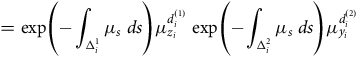 $$ \hskip 70pt= {\rm{exp}}\left( { - \mathop \int \nolimits_{{\rm{\Delta }}_i^1} {\mu _s}{\rm{\;}}ds} \right)\mu _{{z_i}}^{d_i^{\left( 1 \right)}}{\rm{\;exp}}\left( { - \mathop \int \nolimits_{{\rm{\Delta }}_i^2} {\mu _s}{\rm{\;}}ds} \right)\mu _{{y_i}}^{d_i^{\left( 2 \right)}}$$
since necessarily $d_i^{\left( 1 \right)} = 0$
and
$d_i^{\left( 1 \right)} = 0$
and $d_i^{\left( 2 \right)} = {d_i}$
if events on
$d_i^{\left( 2 \right)} = {d_i}$
if events on ${{\rm{\Delta }}_2}$
are not trivially null. Whether we regard this as factorizing a likelihood on
${{\rm{\Delta }}_2}$
are not trivially null. Whether we regard this as factorizing a likelihood on ${{\rm{\Delta }}_i}$
, or multiplying two likelihoods on
${{\rm{\Delta }}_i}$
, or multiplying two likelihoods on ${\rm{\Delta }}_i^1$
and
${\rm{\Delta }}_i^1$
and ${\rm{\Delta }}_i^2$
, does not matter for our purposes.
${\rm{\Delta }}_i^2$
, does not matter for our purposes.
3.4. Rate Intervals, Piecewise-constant Hazards and Age-grouped Data
Recall from Section 2.2 that a rate interval is denoted by ${{\rm{\Delta }}_k}$
. Here let
${{\rm{\Delta }}_k}$
. Here let ${{\rm{\Delta }}_k}$
be the rate interval from integer age
${{\rm{\Delta }}_k}$
be the rate interval from integer age $k$
to age
$k$
to age $k + 1$
, that is,
$k + 1$
, that is, ${{\rm{\Delta }}_k} = \left( {k,k + 1} \right]$
. Age-grouped data may then be denoted by total deaths
${{\rm{\Delta }}_k} = \left( {k,k + 1} \right]$
. Age-grouped data may then be denoted by total deaths ${d_k}$
and total person-years exposure
${d_k}$
and total person-years exposure $E_k^c$
falling within rate interval
$E_k^c$
falling within rate interval ${{\rm{\Delta }}_k}$
.
${{\rm{\Delta }}_k}$
.
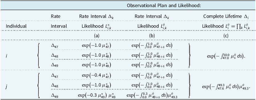
It is instructive to group data on individual lives to reproduce age-grouped data, and to compare the resulting likelihoods. This is aided by Table 2, which shows the contributions to likelihoods of individual data for two individuals, treated three ways. The $i$
th individual is observed from age 47 until right-censored at age 50. The
$i$
th individual is observed from age 47 until right-censored at age 50. The $j$
th individual is observed from age 47.6 until dying at age 49.3. We list contributions to the likelihood under three combinations of observational plan and model:
$j$
th individual is observed from age 47.6 until dying at age 49.3. We list contributions to the likelihood under three combinations of observational plan and model:
-
(a) Rate intervals
${{\rm{\Delta }}_k}$
, and a constant hazard rate on each rate interval, denoted by
$\mu _k^{\rm{*}}$
. -
(b) Rate intervals
${{\rm{\Delta }}_k}$
, and a smooth hazard rate parametrized by
$\theta $
, denoted by
$\mu _x^\theta $
(for example, a Gompertz-Makeham function). -
(c) Observation of complete lifetimes on age interval
${{\rm{\Delta }}_i}$
, and a smooth hazard rate parametrized by
$\theta $
, also denoted by
$\mu _x^\theta $
.


Table 2. Contributions to likelihoods of the $i$
th individual, under observation from age 47 until right-censored at age 50, and the
$i$
th individual, under observation from age 47 until right-censored at age 50, and the $j$
th individual, under observation from age 47.6 until death at age 49.3, under three observational plans and assumptions: (a) annual rate interval
$j$
th individual, under observation from age 47.6 until death at age 49.3, under three observational plans and assumptions: (a) annual rate interval ${{\rm{\Delta }}_k}$
, piecewise-constant hazard rates; (b) annual rate interval
${{\rm{\Delta }}_k}$
, piecewise-constant hazard rates; (b) annual rate interval ${{\rm{\Delta }}_k}$
, smooth hazard rate parametrized by
${{\rm{\Delta }}_k}$
, smooth hazard rate parametrized by $\theta $
; and (c) observation of complete lifetime age interval
$\theta $
; and (c) observation of complete lifetime age interval ${{\rm{\Delta }}_i}$
, smooth hazard rate parametrized by
${{\rm{\Delta }}_i}$
, smooth hazard rate parametrized by $\theta $
The contributions are shown in Table 2. In obvious notation, we may denote the contributions to the likelihoods under (a), (b) and (c) above by $L_{i,k}^{\rm{*}},L_{i,k}^\theta $
and
$L_{i,k}^{\rm{*}},L_{i,k}^\theta $
and $L_i^\theta = \mathop \prod \nolimits_k L_{i,k}^\theta $
respectively. Likewise, collecting all contributions to rate interval
$L_i^\theta = \mathop \prod \nolimits_k L_{i,k}^\theta $
respectively. Likewise, collecting all contributions to rate interval ${{\rm{\Delta }}_k}$
in columns (a) and (b), we may define the total likelihood contributed by
${{\rm{\Delta }}_k}$
in columns (a) and (b), we may define the total likelihood contributed by ${{\rm{\Delta }}_k}$
by
${{\rm{\Delta }}_k}$
by $L_k^{\rm{*}} = \mathop \prod \nolimits_i L_{i,k}^{\rm{*}}$
and
$L_k^{\rm{*}} = \mathop \prod \nolimits_i L_{i,k}^{\rm{*}}$
and ${L_k^{\theta}} = \mathop \prod \nolimits_i {L_{i,k}^{\theta}}$
respectively. This leads to the following observations.
${L_k^{\theta}} = \mathop \prod \nolimits_i {L_{i,k}^{\theta}}$
respectively. This leads to the following observations.
-
(a) It is obvious from columns (b) and (c) in Table 2 that for any individual, the likelihood over the complete lifetime is the product of the likelihoods over each rate interval, see Section 3.3. In fact we have incorporated this in the notation,
$L_i^\theta = \mathop \prod \nolimits_k L_{i,k}^\theta $
. It makes no difference if we split the the individual lives data and present them by rate interval. But this does not lead to any simplification, and age-grouped totals
${d_k}$
and
$E_k^c$
play no part, because of the smooth hazard rate in the integrands. -
(b) Each entry in column (a) of Table 2 can be regarded as approximating its partner in column (b). For example in the third and sixth lines, we approximate
$\mu _{49 + s}^\theta $
by
$\mu _{49}^{\rm{*}}$
for
$0 \lt s \le 1$
; we show the sixth line below:(15)
$${\rm{exp}}\left( { - \mathop \int \nolimits_{0.0}^{0.3} \mu _{49 + s}^\theta {\rm{\;}}ds} \right)\mu _{49.3}^\theta \approx {\rm{exp}}\left( { - \mathop \int \nolimits_{0.0}^{0.3} \mu _{49}^{\rm{*}}{\rm{\;}}ds} \right)\mu _{49}^{\rm{*}} = {\rm{exp}}\left( { - 0.3\mu _{49}^{\rm{*}}} \right)\mu _{49}^{\rm{*}}.$$
Collecting together all such terms in
$\mu _{49}^{\rm{*}}$
we get the total likelihood:(16)
$$L_{49}^{\rm{*}}\left( {\mu _{49}^{\rm{*}}} \right) = {\rm{exp}}\left( { - \mu _{49}^{\rm{*}}{\rm{\;}}E_{49}^c} \right){(\mu _{49}^{\rm{*}})^{{d_{49}}}}$$
in which the age-grouped totals do appear. Comparing equations (16) and (8), we see that the former is functionally identical to the likelihood from the Poisson model, and yet no assumption about Poisson random variables or distributions has been made in this section. In other words, the Poisson-like nature of the likelihood arises from the fundamental nature of modelling individual lifetimes.


3.5. Individual versus Age-Grouped Data for Multiple Lives
Table 2 illustrates how the individual lifetime model is related to age-grouped data, based on rate intervals, exactly without using any approximations. Indeed, columns (b) and (c) show that labelling the data by individual $i$
or by rate interval
$i$
or by rate interval $k$
is merely a rearrangement. Specifically, the
$k$
is merely a rearrangement. Specifically, the $i$
th individual contributes
$i$
th individual contributes $L_{i,k}^\theta $
, possibly null, to the likelihood in rate interval
$L_{i,k}^\theta $
, possibly null, to the likelihood in rate interval $k$
(column (b)). The outer form of the total likelihood, denoted by
$k$
(column (b)). The outer form of the total likelihood, denoted by ${L^\theta }$
, then depends simply on the order in which we take products, as the following identities show:
${L^\theta }$
, then depends simply on the order in which we take products, as the following identities show:
 $${L^\theta } = \mathop \prod \limits_i L_i^\theta = \mathop \prod \limits_i \mathop \prod \limits_k L_{i,k}^\theta = \mathop \prod \limits_k \mathop \prod \limits_i L_{i,k}^\theta = \mathop \prod \limits_k L_k^\theta = {L^\theta }.$$
This informal statement based on Table 2 (“proof-by-example”) of course needs to be demonstrated properly. Doing so with the notation to hand is surprisingly detailed, though elementary, and is delegated to Appendix A. A much simpler proof will be shown when the notation of Section 4 is available (Section 4.7).
3.6. The Rôle of Occurrence-exposure Rates
We may arrive at the likelihood based on the age-grouped data $\left( {{d_k},E_k^c} \right)$
in two different ways.
$\left( {{d_k},E_k^c} \right)$
in two different ways.
-
(a) We could use the Poisson model with parameter
$\mu _k^{\rm{*}}{\rm{\,}}E_k^c$
(Section 2.4) for rate interval
${{\rm{\Delta }}_k}$
. -
(b) Within the individual lives model, we could assume that the hazard rate is piecewise-constant with value
$\mu _k^{\rm{*}}$
on rate interval
${{\rm{\Delta }}_k}$
. This means assuming that the parameter
$\theta $
is the vector of hazard rates
$\mu _k^{\rm{*}}$
.


In either case, on rate interval ${{\rm{\Delta }}_k}$
, we have a single parameter, which we denote by
${{\rm{\Delta }}_k}$
, we have a single parameter, which we denote by $\mu _k^{\rm{*}}$
, and a likelihood that we denote by
$\mu _k^{\rm{*}}$
, and a likelihood that we denote by $L_k^{\rm{*}}\left( {\mu _k^{\rm{*}}} \right) = {\rm{exp}}\left( { - \mu _k^{\rm{*}}{\rm{\,}}E_k^c} \right){\rm{\;}}{(\mu _k^{\rm{*}})^{{d_k}}}$
. In total we have a
$L_k^{\rm{*}}\left( {\mu _k^{\rm{*}}} \right) = {\rm{exp}}\left( { - \mu _k^{\rm{*}}{\rm{\,}}E_k^c} \right){\rm{\;}}{(\mu _k^{\rm{*}})^{{d_k}}}$
. In total we have a $K$
-parameter model with likelihood
$K$
-parameter model with likelihood $\mathop \prod \nolimits_k L_k^{\rm{*}}\left( {\mu _k^{\rm{*}}} \right)$
, from which the parameters are estimated independently by the occurrence-exposure rates
$\mathop \prod \nolimits_k L_k^{\rm{*}}\left( {\mu _k^{\rm{*}}} \right)$
, from which the parameters are estimated independently by the occurrence-exposure rates ${d_k}/E_k^c$
, which we denote by
${d_k}/E_k^c$
, which we denote by $\hat \mu _k^{\rm{*}}$
. That is as far as the probabilistic model takes us.
$\hat \mu _k^{\rm{*}}$
. That is as far as the probabilistic model takes us.
In traditional actuarial terminology, the $\hat \mu _k^{\rm{*}}$
are “crude” rates which require to be smoothed or graduated, using no more than the available age-grouped data (Benjamin & Pollard, Reference Benjamin and Pollard1980). A convenient way of doing so is to use: (a) the likelihood function
$\hat \mu _k^{\rm{*}}$
are “crude” rates which require to be smoothed or graduated, using no more than the available age-grouped data (Benjamin & Pollard, Reference Benjamin and Pollard1980). A convenient way of doing so is to use: (a) the likelihood function $\mathop \prod \nolimits_k L_k^{\rm{*}}\left( {\mu _k^{\rm{*}}} \right)$
; (b) a parametric function
$\mathop \prod \nolimits_k L_k^{\rm{*}}\left( {\mu _k^{\rm{*}}} \right)$
; (b) a parametric function $\mu _x^\theta $
for the hazard rate, of much lower dimension than
$\mu _x^\theta $
for the hazard rate, of much lower dimension than $K$
; and (c) to connect the two with an assumption that
$K$
; and (c) to connect the two with an assumption that $\hat \mu _k^{\rm{*}}$
estimates
$\hat \mu _k^{\rm{*}}$
estimates $\mu _{{x_k}}^\theta $
, for some
$\mu _{{x_k}}^\theta $
, for some ${x_k} \in {{\rm{\Delta }}_k}$
, for example
${x_k} \in {{\rm{\Delta }}_k}$
, for example $\hat \mu _k^{\rm{*}}$
estimates
$\hat \mu _k^{\rm{*}}$
estimates $\mu _{k + 1/2}^\theta $
. Note that this smoothing procedure is not part of the probabilistic model, despite its use of the likelihood function. Forfar et al. (Reference Forfar, McCutcheon and Wilkie1988) show that it is approximately equivalent to the much older minimum-
$\mu _{k + 1/2}^\theta $
. Note that this smoothing procedure is not part of the probabilistic model, despite its use of the likelihood function. Forfar et al. (Reference Forfar, McCutcheon and Wilkie1988) show that it is approximately equivalent to the much older minimum- ${\chi ^2}$
method.
${\chi ^2}$
method.
In either case, again, the age-grouped quantities approximate exact quantities as follows:
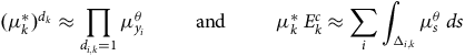 $${(\mu _k^{\rm{*}})^{{d_k}}} \approx \mathop \prod \limits_{{d_{i,k}} = 1} \mu _{{y_i}}^\theta {\rm{\;\;\;\;\;\;\;\;\;and\;\;\;\;\;\;\;\;\;}}\mu _k^{\rm{*}}{\rm{\,}}E_k^c \approx \mathop \sum \limits_i \mathop \int \nolimits_{{{\rm{\Delta }}_{i,k}}} \mu _s^\theta {\rm{\;}}ds$$
where ${d_{i,k}}$
is the number of deaths (0 or 1) befalling the
${d_{i,k}}$
is the number of deaths (0 or 1) befalling the $i$
th individual in rate interval
$i$
th individual in rate interval ${{\rm{\Delta }}_k}$
, and
${{\rm{\Delta }}_k}$
, and ${{\rm{\Delta }}_{i,k}} = {{\rm{\Delta }}_i} \cap {{\rm{\Delta }}_k}$
(possibly
${{\rm{\Delta }}_{i,k}} = {{\rm{\Delta }}_i} \cap {{\rm{\Delta }}_k}$
(possibly $\emptyset $
). Therefore, inference based upon age-grouped data is close, but not identical, to inference based upon the individual lives data.
$\emptyset $
). Therefore, inference based upon age-grouped data is close, but not identical, to inference based upon the individual lives data.
The crude hazard rates $\hat \mu _k^{\rm{*}}$
, or more accurately the expected deaths based upon them,
$\hat \mu _k^{\rm{*}}$
, or more accurately the expected deaths based upon them, $\hat \mu _k^{\rm{*}}{\rm{\,}}E_k^c$
, may be used in forming statistics such as deviances, used in testing the fit of a graduation (Benjamin & Pollard, Reference Benjamin and Pollard1980; Forfar et al., Reference Forfar, McCutcheon and Wilkie1988; Macdonald et al., Reference Macdonald, Richards and Currie2018).
$\hat \mu _k^{\rm{*}}{\rm{\,}}E_k^c$
, may be used in forming statistics such as deviances, used in testing the fit of a graduation (Benjamin & Pollard, Reference Benjamin and Pollard1980; Forfar et al., Reference Forfar, McCutcheon and Wilkie1988; Macdonald et al., Reference Macdonald, Richards and Currie2018).
3.7. Pseudo-Poisson Models
The various likelihoods that appear in this section, see Table 2, are all Poisson-like, and if a piecewise-constant hazard rate is assumed, indistinguishable from a true Poisson likelihood, an observation that goes back to the earliest work on inference in Markov models, see for example Sverdrup (Reference Sverdrup1965); Waters (Reference Waters1984). However, there are no Poisson random variables. In the likelihood (13): (a) ${d_i}$
is either 0 or 1, and does not range over the non-negative integers; (b)
${d_i}$
is either 0 or 1, and does not range over the non-negative integers; (b) ${v_i}$
is random, not deterministic; and (c)
${v_i}$
is random, not deterministic; and (c) ${d_i}$
and
${d_i}$
and ${v_i}$
are not independent, the random variable is the bivariate
${v_i}$
are not independent, the random variable is the bivariate $\left( {{d_i},{v_i}} \right)$
. Many authors suppose, as we did in Section 2.4, that the number of deaths in some model has a Poisson distribution, but without ensuring, as we did, that the exposure times would be non-random; more often the observation of random death times ensures the opposite. This conceptual error is almost always immaterial for inference, precisely because the Poisson likelihood is of the correct form for a survival model, although the survival model is not Poisson. Where it matters is in misdirecting us when we come to extend the survival model, including allowing for: (a) truncation and censoring; (b) more complicated life histories, including multiple decrements; (c) calculating residuals when the expected number of deaths is small; and (d) statistics for multiple lives, see Section 3.5 and Appendix A.
$\left( {{d_i},{v_i}} \right)$
. Many authors suppose, as we did in Section 2.4, that the number of deaths in some model has a Poisson distribution, but without ensuring, as we did, that the exposure times would be non-random; more often the observation of random death times ensures the opposite. This conceptual error is almost always immaterial for inference, precisely because the Poisson likelihood is of the correct form for a survival model, although the survival model is not Poisson. Where it matters is in misdirecting us when we come to extend the survival model, including allowing for: (a) truncation and censoring; (b) more complicated life histories, including multiple decrements; (c) calculating residuals when the expected number of deaths is small; and (d) statistics for multiple lives, see Section 3.5 and Appendix A.
We suggest it would be clearer and less confusing if the term pseudo-Poisson was adopted, to describe the great majority of models for death counts that appear in the literature.
3.8. Covariates
Covariates may be introduced by defining a vector ${{\bf{z}}^i}$
of covariates for the
${{\bf{z}}^i}$
of covariates for the $i$
th individual and letting the hazard rate be a function
$i$
th individual and letting the hazard rate be a function $\mu (x,$
z
$\mu (x,$
z ${^i})$
of age and covariates. A common way to introduce such a dependency is to define a vector
β
of regression coefficients such that the hazard rate is a function
${^i})$
of age and covariates. A common way to introduce such a dependency is to define a vector
β
of regression coefficients such that the hazard rate is a function $\mu (x,{\rm{\;}}{\beta ^T}$
z
$\mu (x,{\rm{\;}}{\beta ^T}$
z ${^i})$
of age and a linear combination of the covariates. Further simplification is achieved if the hazard rate factorizes as
${^i})$
of age and a linear combination of the covariates. Further simplification is achieved if the hazard rate factorizes as $\mu (x,$ $z{{\rm}^i}) = {\mu _x} \times g($
z
$z{{\rm}^i}) = {\mu _x} \times g($
z ${^i})$
, the product of an age dependent hazard rate
${^i})$
, the product of an age dependent hazard rate ${\mu _x}$
(called the baseline hazard) and some function
${\mu _x}$
(called the baseline hazard) and some function $g$
of the covariates; then the hazard rates of any two individuals of the same age are always in the same proportion, called proportional hazards. Finally, the most common choice of
$g$
of the covariates; then the hazard rates of any two individuals of the same age are always in the same proportion, called proportional hazards. Finally, the most common choice of $g$
is an exponential function of a linear combination of the covariates,
$g$
is an exponential function of a linear combination of the covariates, $\mu (x,$
z
$\mu (x,$
z ${^i}) = {\mu _x} \times {\rm{exp}}({\beta ^T}$
z
${^i}) = {\mu _x} \times {\rm{exp}}({\beta ^T}$
z ${^i})$
, which has proportional and non-negative hazards as well as a log-linear dependence on covariates. These steps in adding structure to the hazard rate are summarized in Table 3.
${^i})$
, which has proportional and non-negative hazards as well as a log-linear dependence on covariates. These steps in adding structure to the hazard rate are summarized in Table 3.
Table 3. Three stages in adding structure to a hazard rate that is a function $\mu (x,{{\rm z}^i})$
of age
$\mu (x,{{\rm z}^i})$
of age $x$
and a vector
$x$
and a vector ${{\rm z}^i}$
of covariates for the
${{\rm z}^i}$
of covariates for the $i$
th individual. Each stage is increasingly restrictive, from the most flexible model in Stage 0 to the most restrictive in Stage 3
$i$
th individual. Each stage is increasingly restrictive, from the most flexible model in Stage 0 to the most restrictive in Stage 3
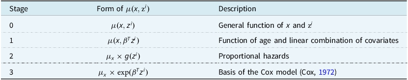
The last hazard structure in Table 3 is popular in medical statistics, where it is known as the Cox model, because the baseline hazard can be ignored and only the regression coefficients need to be estimated, by the procedure known as partial likelihood (see Andersen et al. (Reference Andersen, Borgan, Gill and Keiding1993)). However, actuaries usually wish to estimate the whole model, baseline hazard included, whatever the form of the hazard rate. Then the full likelihood (46) from Appendix A becomes:
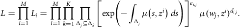 $$L = \mathop \prod \limits_{i = 1}^M {L_i} = \mathop \prod \limits_{i = 1}^M \mathop \prod \limits_{k = 1}^K \mathop \prod \limits_{{{\rm{\Delta }}_j} \subseteq {{\rm{\Delta }}_k}} {\left[ {{\rm{exp}}\left( { - \mathop \int \nolimits_{{{\rm{\Delta }}_j}} \mu \left( {s{,z^i}} \right){\rm{\;}}ds} \right)} \right]^{{e_{i,j}}}}{\rm{\;}}\mu {({w_j}{,z^i})^{{d_{i,j}}}}.$$
Clearly any of the hazard rates in Table 3 may be substituted into the likelihood (19). However inspection of the innermost elements of (19), integrals over intervals ${{\rm{\Delta }}_j} \subseteq {{\rm{\Delta }}_k}$
, shows that, even if the hazard rate factorizes as in Stages 2 and 3 of Table 3, these factors cannot be collected together to form likelihoods
${{\rm{\Delta }}_j} \subseteq {{\rm{\Delta }}_k}$
, shows that, even if the hazard rate factorizes as in Stages 2 and 3 of Table 3, these factors cannot be collected together to form likelihoods ${L_k}$
over rate intervals. See also the written comments by A. D. Wilkie in the discussion of Richards (Reference Richards2008).
${L_k}$
over rate intervals. See also the written comments by A. D. Wilkie in the discussion of Richards (Reference Richards2008).
4. Dynamic Life History Models
4.1. The Anatomy of a Survival Probability
We begin with a closer examination of the multiplicative property of survival probabilities, usually expressed as:
 $${{\rm{\;}}_{s + t}}{p_x} = {_t}{p_x}{{\rm{\;}}_s}{p_{x + t}} = {_s}{p_x}{{\rm{\;}}_t}{p_{x + s}}.$$
We can apply this repeatedly to factorize ${{\rm{\;}}_t}{p_x}$
, with
${{\rm{\;}}_t}{p_x}$
, with $n$
a positive integer, as follows:
$n$
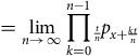
a positive integer, as follows:
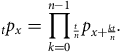 $$_t{p_x} = {\mathop {\prod \limits_{k = 0}^{n - 1}}{_{t \over n}}}\,{p_{x + {{kt} \over n}}}.$$
This motivates the first of two questions: what happens as $n \to \infty $
? The second (related) question is: how can we express or represent events in the life history as a function of passing time? We have a compact notation (
$n \to \infty $
? The second (related) question is: how can we express or represent events in the life history as a function of passing time? We have a compact notation ( ${{\rm}_t}{p_x}$
,
${{\rm}_t}{p_x}$
, ${{\rm{\;}}_t}{q_x}$
and so on) for the probabilities of events in the life history, but no such notation for the events themselves; generally we must express events somewhat clumsily in words. We consider these questions in turn in the next two sections.
${{\rm{\;}}_t}{q_x}$
and so on) for the probabilities of events in the life history, but no such notation for the events themselves; generally we must express events somewhat clumsily in words. We consider these questions in turn in the next two sections.
4.2. The Product-integral Representation of a Survival Probability
From the heuristic ${{\rm{\;}}_h}{p_x} \approx 1 - {\mu _x}{\rm{\,}}h \approx {\rm{exp}}\left( { - {\mu _x}{\rm{\,}}h} \right)$
, for small
${{\rm{\;}}_h}{p_x} \approx 1 - {\mu _x}{\rm{\,}}h \approx {\rm{exp}}\left( { - {\mu _x}{\rm{\,}}h} \right)$
, for small $h$
, we have the important product-integral representation as
$h$
, we have the important product-integral representation as $n \to \infty $
and
$n \to \infty $
and $1/n \to {0^ + }$
:
$1/n \to {0^ + }$
:
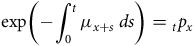 $$\hskip -130pt{\rm{exp}}\left( { - \mathop \int \nolimits_0^t {\mu _{x + s}}{\rm{\;}}ds} \right) = {_t}{p_x}$$
 $$ \hskip -1pt= \mathop {{\rm{lim}}}\limits_{n \to \infty } {\mathop {\prod \limits_{k = 0}^{n - 1}} {_{t \over n}}}{p_{x + {{kt} \over n}}}$$
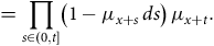
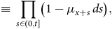 $$\hskip 18pt\equiv \mathop \prod \limits_{s \in \left( {0,t} \right]} \left( {1 - {\mu _{x + s}}{\rm{\,}}ds} \right),$$
see Appendix B or, for example, Andersen et al. (Reference Andersen, Borgan, Gill and Keiding1993). The product-integral has the same ${\rm{\Pi }}$
symbol as an ordinary product over a finite or countable number of terms, but is distinguished (here) by the presence of
${\rm{\Pi }}$
symbol as an ordinary product over a finite or countable number of terms, but is distinguished (here) by the presence of $ds$
in the integrand and by the variable
$ds$
in the integrand and by the variable $s$
ranging over an interval of the real line,
$s$
ranging over an interval of the real line, $s \in \left( {0,t} \right]$
. Then by differentiation of
$s \in \left( {0,t} \right]$
. Then by differentiation of ${{\rm{\;}}_t}{p_x}$
, the density function of the random future lifetime
${{\rm{\;}}_t}{p_x}$
, the density function of the random future lifetime ${T_x}$
, denoted by
${T_x}$
, denoted by ${f_x}\left( t \right)$
, is:
${f_x}\left( t \right)$
, is:
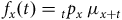 $$\hskip -85pt{f_x}\left( t \right) = {_t}{p_x}{\rm{\;}}{\mu _{x + t}}$$
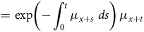 $$= {\rm{exp}}\left( { - \mathop \int \nolimits_0^t {\mu _{x + s}}{\rm{\;}}ds} \right){\rm{\,}}{\mu _{x + t}}$$
 $$\hskip -3pt= \mathop \prod \limits_{s \in \left( {0,t} \right]} \left( {1 - {\mu _{x + s}}{\rm{\,}}ds} \right){\rm{\,}}{\mu _{x + t}}.$$
Identities (26) and (27) are important in parametric mortality models, because they allow the likelihood to be specified entirely in terms of the hazard rate.
4.3. The Counting Process Representation of the Data
Suppose the $i$
th individual has future lifetime
$i$
th individual has future lifetime $T_0^i$
, a non-negative random variable. Define the process
$T_0^i$
, a non-negative random variable. Define the process ${N^i}\left( x \right) = {I_{\left\{ {T_0^i \le x} \right\}}}$
. This has value 0 as long as the
${N^i}\left( x \right) = {I_{\left\{ {T_0^i \le x} \right\}}}$
. This has value 0 as long as the $i$
th individual is alive, and value 1 if they are dead (including at exact age
$i$
th individual is alive, and value 1 if they are dead (including at exact age $T_0^i$
). Thus
$T_0^i$
). Thus ${N^i}\left( x \right)$
“counts” the number of deaths up to and including age
${N^i}\left( x \right)$
“counts” the number of deaths up to and including age $x$
.
$x$
.
Associated with ${N^i}\left( x \right)$
is the indicator of survival, denoted by
${N^i}\left( x \right)$
is the indicator of survival, denoted by ${Y^i}\left( x \right)$
and defined as:
${Y^i}\left( x \right)$
and defined as:
 $${Y^i}\left( x \right) = {I_{\left\{ {i{\rm{th\;individual\;alive\;at\;ag}}e{\rm{\;}}{x^ - }} \right\}}} = {I_{\left\{ {T_0^i \ge x} \right\}}}.$$
Thus ${Y^i}\left( x \right)$
is almost, but not quite, equal to
${Y^i}\left( x \right)$
is almost, but not quite, equal to $1 - {N^i}\left( x \right)$
. Both have value 1 at exact age
$1 - {N^i}\left( x \right)$
. Both have value 1 at exact age $x = T_0^i$
, the age at death (see Table 4).
$x = T_0^i$
, the age at death (see Table 4). ${N^i}\left( x \right)$
is right-continuous, while
${N^i}\left( x \right)$
is right-continuous, while ${Y^i}\left( x \right)$
is left-continuous. This is for technical reasons when forming integrals.
${Y^i}\left( x \right)$
is left-continuous. This is for technical reasons when forming integrals.
Table 4. Contributions to the probability function of the infinitesimal Bernoulli trials (equation (29)) from elements of the observed life history, in the absence of left-truncation and right-censoring, and in their presence. Technical point: ${N^i}\left( s \right)$
has right-continuous sample paths and
${N^i}\left( s \right)$
has right-continuous sample paths and ${Y^i}\left( s \right)$
has left-continuous sample paths (Section 4.3), so at the time of an observed death
${Y^i}\left( s \right)$
has left-continuous sample paths (Section 4.3), so at the time of an observed death ${N^i}\left( s \right) = {Y^i}\left( s \right) = 1$
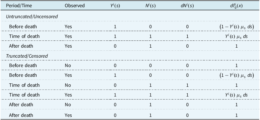
Note that ${N^i}\left( x \right)$
represents exactly the same information as
${N^i}\left( x \right)$
represents exactly the same information as $T_0^i$
, but in the form of a stochastic process instead of a random variable. It is purely descriptive, no probabilities or hazard rates appear in its definition, hence we refer to the counting process “representation,” not the counting process “model.”
$T_0^i$
, but in the form of a stochastic process instead of a random variable. It is purely descriptive, no probabilities or hazard rates appear in its definition, hence we refer to the counting process “representation,” not the counting process “model.”
Mention the word “process” to an actuary under the age of about fifty, and it will trigger thoughts of Brownian motion, Itô calculus, stochastic integrals and option pricing. While important and necessary in its place, a counting processes carries none of that baggageFootnote 2 . It really is nothing but a parsimonious way to represent an event happening at a random time, by means of zeros and ones. It must have been re-invented hundreds of times by computer programmers needing to represent events in binary.
Nevertheless, with ${N^i}\left( x \right)$
and
${N^i}\left( x \right)$
and ${Y^i}\left( x \right)$
representing the data, and
${Y^i}\left( x \right)$
representing the data, and ${\mu _x}$
as a model of the underlying “mechanism” generating the data, we have the key to many problems of survival models.
${\mu _x}$
as a model of the underlying “mechanism” generating the data, we have the key to many problems of survival models.
4.4. The Multiplicative Model
Just above, we called ${\mu _x}$
the “
${\mu _x}$
the “ $ \ldots $
model of the underlying “mechanism” generating the data
$ \ldots $
model of the underlying “mechanism” generating the data $ \ldots $
”, referring of course to the heuristic, that the probability of death occurring between ages
$ \ldots $
”, referring of course to the heuristic, that the probability of death occurring between ages $x$
and
$x$
and $x + h$
, conditional on not having occurred beforehand, is approximately
$x + h$
, conditional on not having occurred beforehand, is approximately ${\mu _x}{\rm{\,}}h$
(for small
${\mu _x}{\rm{\,}}h$
(for small $h$
). In fact, we make a small adjustment with a truly profound effect.
$h$
). In fact, we make a small adjustment with a truly profound effect.
Define the stochastic hazard rate at age $x$
to be the product
$x$
to be the product ${Y^i}\left( x \right){\rm{\,}}{\mu _x}$
, also called the Aalen multiplicative model (Andersen et al., Reference Andersen, Borgan, Gill and Keiding1993) (both names derive from the fact that the hazard rate is multiplied by a stochastic indicator). This represents a hazard rate tailored to the
${Y^i}\left( x \right){\rm{\,}}{\mu _x}$
, also called the Aalen multiplicative model (Andersen et al., Reference Andersen, Borgan, Gill and Keiding1993) (both names derive from the fact that the hazard rate is multiplied by a stochastic indicator). This represents a hazard rate tailored to the $i$
th individual, that is automatically switched “on” while they are alive and “off” at any other time. Where before, we have had to qualify almost everything we said with the mantra “conditional on the life being alive at age
$i$
th individual, that is automatically switched “on” while they are alive and “off” at any other time. Where before, we have had to qualify almost everything we said with the mantra “conditional on the life being alive at age $x$
” or the like, this is taken care of by the stochastic hazard rate. This explains the title “Dynamic Life History Models” of this section; the hazard rates that govern the evolution of the life history are themselves stochastic and changed by events.
$x$
” or the like, this is taken care of by the stochastic hazard rate. This explains the title “Dynamic Life History Models” of this section; the hazard rates that govern the evolution of the life history are themselves stochastic and changed by events.
4.5. The Stochastic Probability Function: Back to Bernoulli
The probability function of the life history up to age $x$
, from equation (27), in its product-integral form, can be denoted by
$x$
, from equation (27), in its product-integral form, can be denoted by $f_0^i\left( x \right)$
and written as:
$f_0^i\left( x \right)$
and written as:
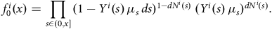 $$f_0^i\left( x \right) = \mathop \prod \limits_{s \in \left( {0,x} \right]} {(1 - {Y^i}\left( s \right){\rm{\,}}{\mu _s}{\rm{\,}}ds)^{1 - d{N^i}\left( s \right)}}{\rm{\;}}{({Y^i}\left( s \right){\rm{\,}}{\mu _s})^{d{N^i}\left( s \right)}}.$$
This says, heuristically, that times when the $i$
th individual does not die (
$i$
th individual does not die ( $d{N^i}\left( s \right) = 0$
) contribute a survival probability
$d{N^i}\left( s \right) = 0$
) contribute a survival probability $\left( {1 - {\mu _s}{\rm{\,}}ds} \right)$
to the product, while the moment of death (
$\left( {1 - {\mu _s}{\rm{\,}}ds} \right)$
to the product, while the moment of death ( $d{N^i}\left( s \right) = 1$
) contributes the death probability
$d{N^i}\left( s \right) = 1$
) contributes the death probability ${\mu _s}{\rm{\,}}ds$
(but by convention the
${\mu _s}{\rm{\,}}ds$
(but by convention the $ds$
is not displayed, as
$ds$
is not displayed, as $f_0^i\left( s \right)$
is then a density function). (In this case the presence of
$f_0^i\left( s \right)$
is then a density function). (In this case the presence of ${Y^i}\left( s \right)$
makes no difference, because the exponents
${Y^i}\left( s \right)$
makes no difference, because the exponents $1 - d{N^i}\left( s \right)$
and
$1 - d{N^i}\left( s \right)$
and $d{N^i}\left( s \right)$
do the job by themselves, but we shall see why it is present in Section 4.6 below. It does matter, however, that
$d{N^i}\left( s \right)$
do the job by themselves, but we shall see why it is present in Section 4.6 below. It does matter, however, that ${Y^i}\left( x \right) = d{N^i}\left( x \right) = 1$
when
${Y^i}\left( x \right) = d{N^i}\left( x \right) = 1$
when $x$
is the age at death.) Table 4 (“Untruncated/Uncensored”) shows the contributions to the likelihood (29) at different points in the observed life history.
$x$
is the age at death.) Table 4 (“Untruncated/Uncensored”) shows the contributions to the likelihood (29) at different points in the observed life history.
In other words, at every time $s$
when the
$s$
when the $i$
th individual is alive there is an infinitesimal Bernoulli trial with probability of death
$i$
th individual is alive there is an infinitesimal Bernoulli trial with probability of death ${Y^i}\left( s \right){\rm{\,}}{\mu _s}{\rm{\,}}ds$
. See Gill (Reference Gill and Bernard1994) on an infinite Bernoulli process. Some authors make product integration the starting point of survival analysis (Cox & Oakes, Reference Cox and Oakes1984; Kalbfleisch & Prentice, Reference Kalbfleisch and Prentice2002; Lancaster, Reference Lancaster1990). Actuaries are so strongly oriented towards binomial and Poisson models, however, that we have approached product integration from there.
${Y^i}\left( s \right){\rm{\,}}{\mu _s}{\rm{\,}}ds$
. See Gill (Reference Gill and Bernard1994) on an infinite Bernoulli process. Some authors make product integration the starting point of survival analysis (Cox & Oakes, Reference Cox and Oakes1984; Kalbfleisch & Prentice, Reference Kalbfleisch and Prentice2002; Lancaster, Reference Lancaster1990). Actuaries are so strongly oriented towards binomial and Poisson models, however, that we have approached product integration from there.
4.6. Left-truncation and Right-censoring
Left-truncation arises when the first part of a lifetime is unobserved. It is a fundamental characteristic of actuarial data, given that the vast majority of insured lives only become known to the insurer as adults. Right-censoring arises when the lifetime leaves observation before the event of interest (such as death) has occurred. There are many causes of right-censoring; Richards and Macdonald (Reference Richards and Macdonald2025) discuss a wide range of right-censoring events in the context of pensions and annuities.
Left-truncation and right-censoring can, in most cases, be allowed for very simply by adjusting the definition of the indicator ${Y^i}\left( s \right)$
, as follows:
${Y^i}\left( s \right)$
, as follows:
 $${Y^i}\left( s \right) = {I_{\left\{ {i{\rm{th\;individual\;alive\;and\;under\;observation\;at\;age\;}}{s^ - }} \right\}}}.$$
With this change, everything said in Sections 4.1 to 4.5, including the important representation in equation (29), remains valid. Table 4 (“Truncated/Censored”) shows the contributions to the likelihood (29) at different points in the observed and unobserved life history, where ${Y^i}\left( s \right)$
indicates the presence of left-truncation and right-censoring by taking the value 0. Equation (29) as defined in Section 4.5 describes a purely mathematical probabilistic model. Substituting the indicator processes in equation (30) turns it into the basis of a statistical model involving data.
${Y^i}\left( s \right)$
indicates the presence of left-truncation and right-censoring by taking the value 0. Equation (29) as defined in Section 4.5 describes a purely mathematical probabilistic model. Substituting the indicator processes in equation (30) turns it into the basis of a statistical model involving data.
Figure 1 shows values of ${Y^i}\left( x \right)$
and
${Y^i}\left( x \right)$
and ${N^i}\left( x \right)$
for two individuals. In the first row, we see observation of the complete lifetime
${N^i}\left( x \right)$
for two individuals. In the first row, we see observation of the complete lifetime $T_0^i$
from birth to death, here at age 81. This illustrates the
$T_0^i$
from birth to death, here at age 81. This illustrates the ${Y^i}\left( x \right)$
of equation (28). In the second row, one who enters observation at age 35 (left-truncation) and leaves without dying at age 45 (right-censoring), then re-enters observation at age 55 (left-truncation) and dies at age 72. This could happen if, for example, extracts from two different policy files are found during data cleaning to refer to the same individual. This illustrates the
${Y^i}\left( x \right)$
of equation (28). In the second row, one who enters observation at age 35 (left-truncation) and leaves without dying at age 45 (right-censoring), then re-enters observation at age 55 (left-truncation) and dies at age 72. This could happen if, for example, extracts from two different policy files are found during data cleaning to refer to the same individual. This illustrates the ${Y^i}\left( x \right)$
of equation (30).
${Y^i}\left( x \right)$
of equation (30).
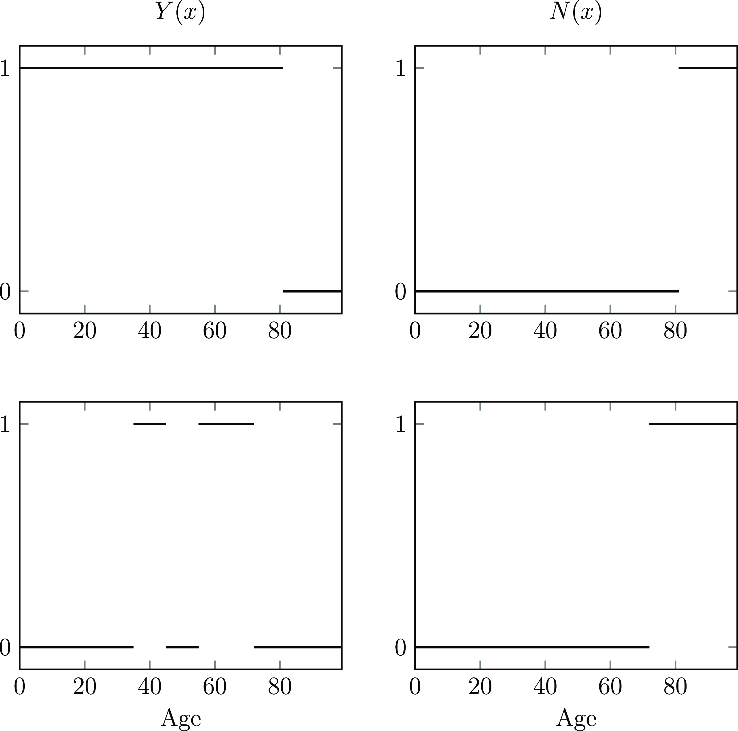
Figure 1. Sample counting process representations of lifetimes. The first row is a life that enters observation at age 0 and is observed until dying at age 81. The second row is a life that enters observation at age 35 (left-truncation) and leaves at age 45 (right-censoring), enters observation again at age 55 (left-truncation) and is then observed until death at age 72.
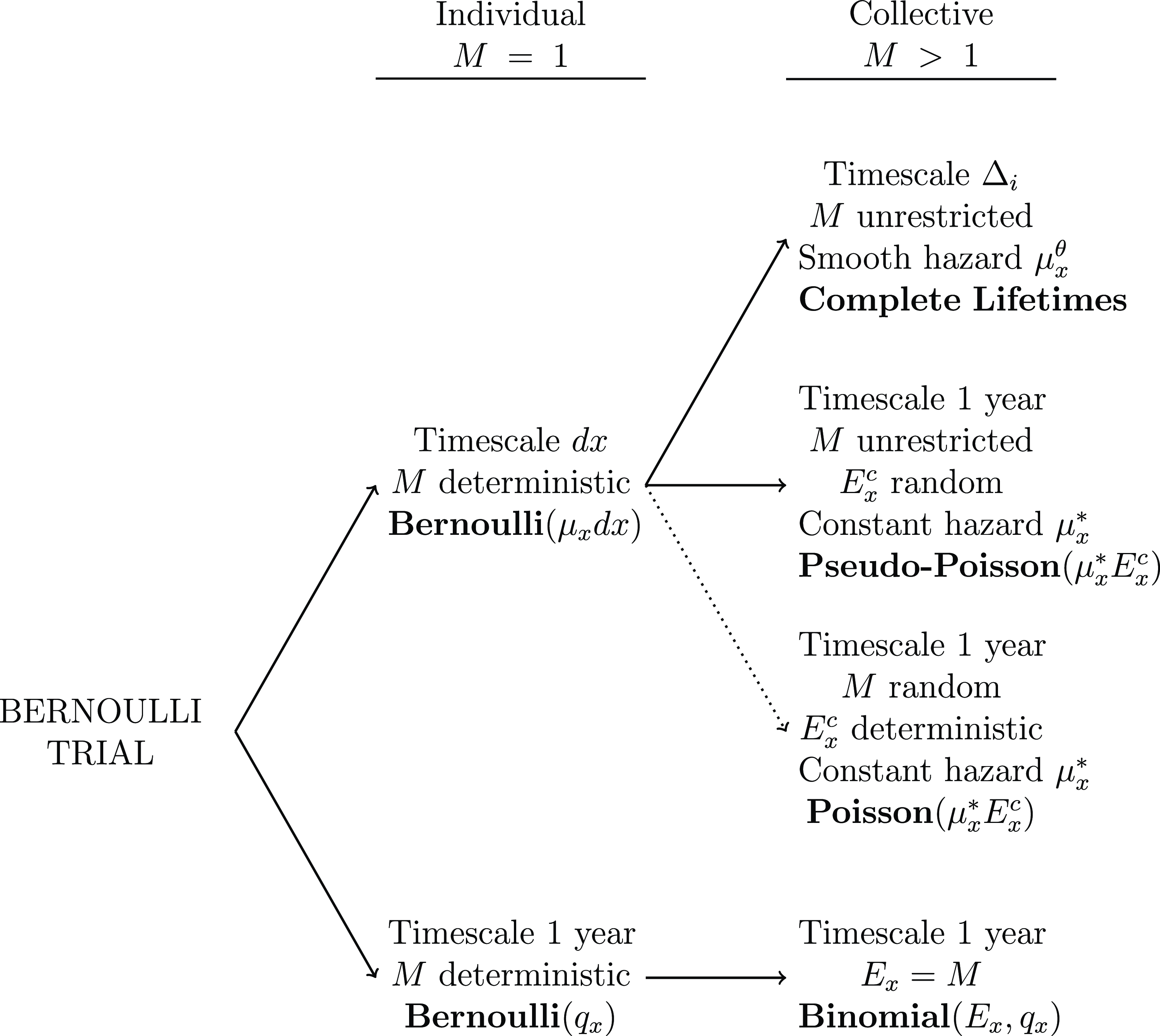
Figure 2. Family tree of models (see Section 4.8) showing the derivation of individual models, and collective models for individual lives and age-grouped data, (in bold) from the basic Bernoulli trial. $M$
is the number of individuals observed, “
$M$
is the number of individuals observed, “ $M$
unrestricted” means that
$M$
unrestricted” means that $M$
can be either random or deterministic. The tree has two branches, one at the top leading to continuous-time models, including pseudo-Poisson and Poisson models, and one at the bottom leading to the discrete-time binomial model. The dotted arrow indicates that the Poisson model requires the imposition of an observational plan that ensures
$M$
can be either random or deterministic. The tree has two branches, one at the top leading to continuous-time models, including pseudo-Poisson and Poisson models, and one at the bottom leading to the discrete-time binomial model. The dotted arrow indicates that the Poisson model requires the imposition of an observational plan that ensures $E_x^{c}$
is deterministic, which is unlikely to be realized in practice.
$E_x^{c}$
is deterministic, which is unlikely to be realized in practice.
The impact of this change in simplifying the mathematics is more than its apparent innocence would suggest. An example will be seen in Section 4.7.
4.7. Example: Individual versus Age-grouped Data for Multiple Lives Again
In Section 3.5 and Appendix A we showed that the likelihoods for individual and age-grouped data were the same, and pseudo-Poisson in form. The method was to derive contributions to the likelihood arising from the smallest possible “units” of exposure to risk, namely the intersection of the $i$
th individual’s lifetime and the
$i$
th individual’s lifetime and the $k$
th rate interval. The total likelihood was then the product of all these “unit” likelihoods over all individuals and all rate intervals. The proof in Appendix A is not technically difficult, but is burdened with the notation needed to define intervals and their intersections. By way of contrast we give below an alternative proof using the counting process representation of the data.
$k$
th rate interval. The total likelihood was then the product of all these “unit” likelihoods over all individuals and all rate intervals. The proof in Appendix A is not technically difficult, but is burdened with the notation needed to define intervals and their intersections. By way of contrast we give below an alternative proof using the counting process representation of the data.
The contribution of the $i$
th individual to the likelihood is:
$i$
th individual to the likelihood is:
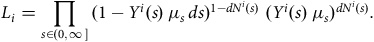 $${L_i} = \mathop \prod \limits_{s \in \left( {0,\infty } \right]} {(1 - {Y^i}\left( s \right){\rm{\,}}{\mu _s}{\rm{\,}}ds)^{1 - d{N^i}(s)}}{\rm{\;}}{({Y^i}\left( s \right){\rm{\,}}{\mu _s})^{d{N^i}\left( s \right)}}.$$
Therefore the total likelihood is:
 $$L = \mathop \prod \limits_i {L_i} = \mathop \prod \limits_i \mathop \prod \limits_{s \in \left( {0,\infty } \right]} {(1 - {Y^i}\left( s \right){\rm{\,}}{\mu _s}{\rm{\,}}ds)^{1 - d{N^i}\left( s \right)}}{\rm{\;}}{({Y^i}\left( s \right){\rm{\,}}{\mu _s})^{d{N^i}\left( s \right)}}.$$
Split the age range into rate intervals ${{\rm{\Delta }}_k}$
, noting that there is no contribution outside the age range
${{\rm{\Delta }}_k}$
, noting that there is no contribution outside the age range $\left[ {{r_0},{r_{K}}} \right]$
:
$\left[ {{r_0},{r_{K}}} \right]$
:
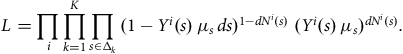 $$L = \mathop \prod \limits_i \mathop \prod \limits_{k = 1}^K \mathop \prod \limits_{s \in {{\rm{\Delta }}_k}} {(1 - {Y^i}\left( s \right){\rm{\,}}{\mu _s}{\rm{\,}}ds)^{1 - d{N^i}\left( s \right)}}{\rm{\;}}{({Y^i}\left( s \right){\rm{\,}}{\mu _s})^{d{N^i}\left( s \right)}}.$$
Now change the order of the two outer products:
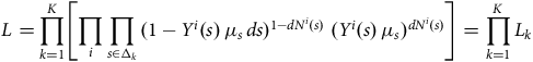 $$L = \mathop \prod \limits_{k = 1}^K \left[ {\mathop \prod \limits_i \mathop \prod \limits_{s \in {{\rm{\Delta }}_k}} {{(1 - {Y^i}\left( s \right){\rm{\,}}{\mu _s}{\rm{\,}}ds)}^{1 - d{N^i}\left( s \right)}}{\rm{\;}}{{({Y^i}\left( s \right){\rm{\,}}{\mu _s})}^{d{N^i}\left( s \right)}}} \right] = \mathop \prod \limits_{k = 1}^K {L_k}$$
noting that the terms in large brackets in (34) are the contributions from each rate intervalFootnote
3
, which we denote by ${L_k}$
.
${L_k}$
.
The simplicity and directness of the proof above arises from the simplicity of the range of integration of the innermost integral, namely 0 to $\infty $
instead of an interval defined by the intersection of two other intervals, see Appendix A. This reinforces an observation by Lidstone (Reference Lidstone1905) to the effect that it may be simpler to investigate what happens moment-by-moment, rather than over an extended interval:
$\infty $
instead of an interval defined by the intersection of two other intervals, see Appendix A. This reinforces an observation by Lidstone (Reference Lidstone1905) to the effect that it may be simpler to investigate what happens moment-by-moment, rather than over an extended interval:
“ $ \ldots $
it will be found that the formulae are in reality simplified through the absence of any distinction between the beginning and end of the momently intervals under consideration.” (Lidstone, Reference Lidstone1905)
$ \ldots $
it will be found that the formulae are in reality simplified through the absence of any distinction between the beginning and end of the momently intervals under consideration.” (Lidstone, Reference Lidstone1905)
Of course, the work in actually computing such complicated integrals is unchanged, but the greater ease of comprehension makes the task of the theorist (and the reader!) much easier.
4.8. A Classification of Mortality Models for Actuarial Use
Figure 2 illustrates how the models underlying survival analysis and occurrence-exposure rates used by actuaries all derive from Bernoulli trials over different time intervals.
-
(a) The upper branch goes through the instantaneous Bernoulli trial with parameter
${\mu _x}{\rm{\,}}dx$
. Then product integration over such Bernoulli “atoms,” selected by the observational plan, embodied in variants of the process
${Y^i}\left( s \right)$
, leads to a Poisson-like likelihood. -
(b) The simplest such observational scheme (upper-top branch in Figure 2) is observation of the
$i$
th individual over the whole age interval
${{\rm{\Delta }}_i}$
. Then simple aggregation over
$M \gt 1$
individuals leads to the survival model based on individual lives: see equation (32) with a parametric hazard rate
$\mu _t^\theta $
:(35)
$$L = \mathop \prod \limits_i {L_i} = \mathop \prod \limits_i \mathop \prod \limits_{s \in \left( {0,\infty } \right]} {(1 - {Y^i}\left( s \right){\rm{\,}}\mu _s^\theta {\rm{\,}}ds)^{1 - d{N^i}\left( s \right)}}{\rm{\;}}{({Y^i}\left( s \right){\rm{\,}}\mu _s^\theta )^{d{N^i}\left( s \right)}}.$$
-
(c) Similarly, product integration restricted to the rate interval
${{\rm{\Delta }}_k}$
, and a constant hazard rate
$\mu _k^{\rm{*}}$
on
${{\rm{\Delta }}_k}$
(upper-middle branch in Figure 2), leads to the pseudo-Poisson model. To make the indicator
${Y^i}\left( t \right)$
“do the work” define:(36)
$$Y_k^i\left( s \right) = {I_{\left\{ {i{\rm{th\;individual\;alive\;and\;under\;observation\;at\;age\;}}{s^ - }{\rm{\;}}for{\rm{\;}}s{\rm{\;}} \in {\rm{\;}}{{\rm{\Delta }}_k}} \right\}}}$$
and then equation (34) becomes:
(37)
$$L = \mathop \prod \limits_{k = 1}^K \left[\mathop \prod \limits_i \mathop \prod \limits_{s \in ( {0,\infty } ]} {(1 - Y_k^i( s){\rm{\,}}\mu _k^{\rm{*}}{\rm{\,}}ds)^{1 - d{N^i}( s)}}{\rm{\;}}( {Y_k^i( s){\rm{\,}}\mu _k^{\rm{*}}{)^{d{N^i}\left( s \right)}}} \right].$$
-
(d) The Poisson model also belongs to the upper branch, but would require a special (and highly unlikely) observational plan to ensure that exposures are deterministic and numbers of deaths are random (upper-bottom branch in Figure 2, with dotted arrow). An example would be to replace each individual who dies with an identical individual until the exposure reaches a pre-determined level (Scott, Reference Scott1982). Such a scheme would require a random number of deaths
${D_k}$
on each interval
${{\rm{\Delta }}_k}$
, and indicators:(38)
$$\tilde Y_k^i\left( s \right) = {I_{\left\{ {i{\rm{th\;individual\;alive\;and\;under\;observation\;at\;age\;}}{s^ - }{\rm{\;}}for{\rm{\;}}s{\rm{\;}} \in {\rm{\;}}{{\rm{\Delta }}_k}} \right\}}}$$
constrained so that, on each interval
${{\rm{\Delta }}_k}$
the total exposure
$E_k^c$
is a predetermined amount:(39)
$$\mathop \sum \limits_i \mathop \int \nolimits_0^\infty \tilde Y_k^i\left( s \right){\rm{\,}}ds = E_k^c.$$
Then the probability of the observed data, an analogue of equation (34), would be:
$$\hskip-50.5pt{P = \mathop \prod \limits_{k = 1}^K {{{{(E_k^c)}^{{D_k}}}} \over {{D_k}!}}{\rm{\;}} \left[\mathop \prod \limits_{i} \mathop \prod \limits_{s \in ( {0,\infty } ]} {(1 - \tilde Y_k^i(s){\rm{\,}}\mu _k^{\rm{*}}{\rm{\,}}ds)^{1 - d{N^i}(s)}}{\rm{\;}}( {\tilde Y_k^i (s){\rm{\,}}\mu _k^{\rm{*}}{)^{d{N^i}(s)}}}\right]}$$
(40)
$$= {\rm{\;constant\;}} \times \mathop \prod \limits_{k = 1}^K \left[\mathop \prod \limits_i \mathop \prod \limits_{s \in ( {0,\infty } ]} {(1 - \tilde Y_k^i( s){\rm{\,}}\mu _k^{\rm{*}}{\rm{\,}}ds)^{1 - d{N^i}( s)}}{\rm{\;}}( {\tilde Y_k^i( s){\rm{\,}}\mu _k^{\rm{*}}{)^{d{N^i}\left( s \right)}}} \right],$$
a product of true Poisson probabilities (not just likelihoods).
-
(e) The lower branch goes through the Bernoulli trial with parameter
${q_x}$
and leads to the binomial model with
$M \gt 1$
individuals.


Thus the upper branch of Figure 2 illustrates our answer to the question: what do we mean by a continuous-time model? That answer is: the family of models with Poisson-like likelihoods built up by product integration from infinitesimal Bernoulli “atoms.”
Note that both branches lose information about which individuals died in going from the individual model ( $M = 1$
) to the collective model (
$M = 1$
) to the collective model ( $M \gt 1$
) but this will not matter for inference since the likelihood will be changed only by a factor not involving the parameter (for example, in the lower branch, a binomial coefficient). Only in the lower branch, however, is information also lost about the times of death, and therefore the true total of person-years lived. This is genuine loss of information which matters for inference, leading us to prefer any of the models in the upper branch over the binomial model.
$M \gt 1$
) but this will not matter for inference since the likelihood will be changed only by a factor not involving the parameter (for example, in the lower branch, a binomial coefficient). Only in the lower branch, however, is information also lost about the times of death, and therefore the true total of person-years lived. This is genuine loss of information which matters for inference, leading us to prefer any of the models in the upper branch over the binomial model.
4.9. Extension to Multiple Decrements
Equation (29) is easily extended to multiple-state models, with a set of states labelled $1,2, \ldots, K$
. Omitting detailed definitions, process
$1,2, \ldots, K$
. Omitting detailed definitions, process $Y_j^i\left( x \right)$
indicates observed presence in state
$Y_j^i\left( x \right)$
indicates observed presence in state $j$
, and process
$j$
, and process $N_{jk}^i\left( x \right)$ $\left( {j \ne k} \right)$
counts transitions from state
$\left( {j \ne k} \right)$
counts transitions from state $j$
to state
$j$
to state $k$
, governed by stochastic intensity
$k$
, governed by stochastic intensity $Y_j^i\left( x \right){\rm{\,}}{\mu _{jk}}\left( x \right)$
, and everything proceeds as before. We will not pursue this in its full generality, referring the reader to Macdonald et al. (Reference Macdonald, Richards and Currie2018) (elementary) or Andersen et al. (Reference Andersen, Borgan, Gill and Keiding1993) (advanced), but the simplicity of this extension is an attractive feature of the counting process representation.
$Y_j^i\left( x \right){\rm{\,}}{\mu _{jk}}\left( x \right)$
, and everything proceeds as before. We will not pursue this in its full generality, referring the reader to Macdonald et al. (Reference Macdonald, Richards and Currie2018) (elementary) or Andersen et al. (Reference Andersen, Borgan, Gill and Keiding1993) (advanced), but the simplicity of this extension is an attractive feature of the counting process representation.
However we will sketch briefly the extension to multiple decrement models, since this has been a staple of actuarial textbooks. We have one originating state, labelled 1, in which all life histories begin, and $K - 1$
decrement states, labelled
$K - 1$
decrement states, labelled $2,3, \ldots, K$
. Transitions are possible from state 1 to any decrement state, governed by intensity
$2,3, \ldots, K$
. Transitions are possible from state 1 to any decrement state, governed by intensity $Y_1^i\left( x \right){\rm{\,}}{\mu _{1k}}\left( x \right)$
for the
$Y_1^i\left( x \right){\rm{\,}}{\mu _{1k}}\left( x \right)$
for the $i$
th individualFootnote
4
. Figure 3 illustrates this model. Intensities out of a given state are additive, so exit from state 1 is represented by the counting process
$i$
th individualFootnote
4
. Figure 3 illustrates this model. Intensities out of a given state are additive, so exit from state 1 is represented by the counting process $N_{1 \bullet }^i\left( x \right) = N_{12}^i\left( x \right) + \ldots + N_{1K}^i\left( x \right)$
, governed by the total intensity, denoted by
$N_{1 \bullet }^i\left( x \right) = N_{12}^i\left( x \right) + \ldots + N_{1K}^i\left( x \right)$
, governed by the total intensity, denoted by ${\mu _{1 \bullet }}\left( x \right)$
, defined as
${\mu _{1 \bullet }}\left( x \right)$
, defined as ${\mu _{1 \bullet }}\left( x \right) = {\mu _{12}}\left( x \right) + \ldots, + {\mu _{1K}}\left( x \right)$
. The probability function of the life history can be expressed in two rules:
${\mu _{1 \bullet }}\left( x \right) = {\mu _{12}}\left( x \right) + \ldots, + {\mu _{1K}}\left( x \right)$
. The probability function of the life history can be expressed in two rules:
-
Rule 1: The time of exit of the
$i$
th individual from state 1 has probability function similar to equation (29):

 $${f^i}\left( x \right) = \mathop \prod \limits_{s \in \left( {0,x} \right]} {(1 - Y_1^i\left( s \right){\rm{\,}}{\mu _{1 \bullet }}\left( s \right){\rm{\,}}ds)^{1 - dN_{1 \bullet }^i\left( s \right)}}{\rm{\;}}{(Y_1^i\left( s \right){\rm{\,}}{\mu _{1 \bullet }}\left( s \right))^{dN_{1 \bullet }^i\left( s \right)}}.$$
-
Rule 2: Conditional on the
$i$
th individual exiting state 1 at age
$x$
, the probability that the state entered was
$k$
is
${\mu _{1k}}\left( x \right)/{\mu _{1 \bullet }}\left( x \right)$
,
$k = 2, \ldots, K$
.


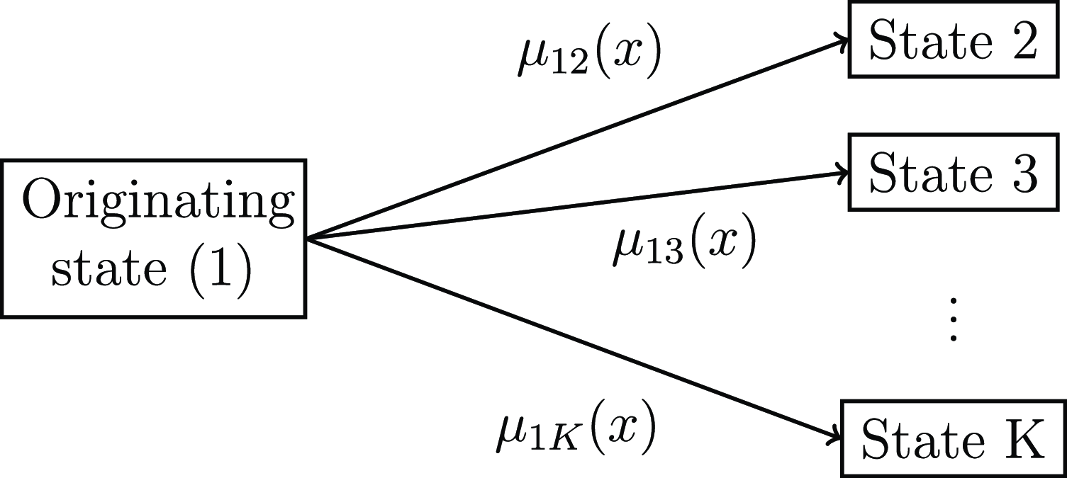
Figure 3. Multiple-decrement model. Note that states $2,3, \ldots, K$
are absorbing states with no transitions out once entered.
$2,3, \ldots, K$
are absorbing states with no transitions out once entered.
Therefore the model is specified completely by a product of infinitesimal Bernoulli trials as in Rule 1, and a simple ratio of intensities as in Rule 2.
If, however, the analyst begins by specifying a binomial-type model, for example based on a time unit of a year, then it is not easy to obtain a convincing representation of behaviour over shorter time periods, and there is certainly no unique solution. The classical actuarial approach (see Neill (Reference Neill1977) or Bowers et al. (Reference Bowers, Gerber, Hickman, Jones and Nesbitt1997)) involves specifying a hypothetical model of each decrement acting alone, leading to a “gross” hazard rate acting in the presence of the other decrements, and a “net” hazard rate acting in their absenceFootnote 5 . Except in some special cases, further progress is impossible unless “gross” and “net” hazard rates are assumed to be equal, but then since “gross” hazard rates can be shown to be those of the Markov multiple-state model anyway, the modeller is drawn ineluctably towards that destination. Going into more detail would require too much notation, see Macdonald et al. (Reference Macdonald, Richards and Currie2018), Chapter 16.
This illustrates vividly the contrast between the simplicity of the model specified at the “micro” level, from which, by aggregation, behaviour at the “macro” level can be deduced; and the perils of specifying the model at the “macro” level, and then trying to disaggregate it to deduce or intuit behaviour on smaller scales.
4.10. Further Applications
We mentioned in Section 4.9 the extension of the counting process representation to multiple-state models, see Macdonald et al. (Reference Macdonald, Richards and Currie2018). We mention here other advances and applications based on counting processes, which can be found in the references below:
-
(a) counting process compensators, martingales, stochastic integrals and central limit theorems (Andersen et al., Reference Andersen, Borgan, Gill and Keiding1993, Chapter III);
-
(b) non-parametric estimates including the Nelson-Aalen and Kaplan-Meier estimates (Andersen et al., Reference Andersen, Borgan, Gill and Keiding1993, Chapters IV.1 and IV.3), (Kalbfleisch & Prentice, Reference Kalbfleisch and Prentice2002);
-
(c) non-parametric kernel smoothing methods (Andersen et al., Reference Andersen, Borgan, Gill and Keiding1993, Chapter IV.2);
-
(d) semi-parametric regression models including the Cox model and partial likelihoods (Andersen et al., Reference Andersen, Borgan, Gill and Keiding1993, Chapter VII), (Kalbfleisch & Prentice, Reference Kalbfleisch and Prentice2002);
-
(e) log-rank comparison tests of survival models (Andersen et al., Reference Andersen, Borgan, Gill and Keiding1993, Chapter V), (Kalbfleisch & Prentice, Reference Kalbfleisch and Prentice2002);
-
(f) stochastic reserving models in life insurance Norberg (Reference Norberg1991); and
-
(g) stochastic models of surplus in life insurance, including Hattendorff’s theorem (Norberg, Reference Norberg1991; Ramlau-Hansen, Reference Ramlau-Hansen1988 a, Reference Ramlau-Hansen1988 b).
5. Conclusions
In search of sound foundations for mortality models, we began with binomial and Poisson models for grouped counts (Section 2), the basis of traditional graduations of mortality data for actuarial use. Both being models for “count” data – the number of deaths during a time period, typically a year – they naturally invite questions about mortality at a smaller scale, over a fraction of the time unit. The Poisson model has an answer; its parameter is a hazard rate ${\mu _x}$
, assumed to be constant over the time period, and that defines mortality over short time intervals
${\mu _x}$
, assumed to be constant over the time period, and that defines mortality over short time intervals $h$
as
$h$
as $h \to {0^ + }$
. The binomial model has no such answer; it is up to the modeller to assume how mortality behaves over shrinking time intervals
$h \to {0^ + }$
. The binomial model has no such answer; it is up to the modeller to assume how mortality behaves over shrinking time intervals $h$
as
$h$
as $h \to {0^ + }$
. While this is unsatisfactory, the binomial model does decompose into a sum of Bernoulli trials, each representing the mortality of an individual over the time period.
$h \to {0^ + }$
. While this is unsatisfactory, the binomial model does decompose into a sum of Bernoulli trials, each representing the mortality of an individual over the time period.
Modelling the lifetime of a single individual (Section 3) gives the vital insight that the associated likelihood, as in equation (13), has the same form as a Poisson likelihood. Indeed we get the same Poisson-like likelihood if we model individual life histories, or group the data by age (Section 3.5), but in neither case do Poisson random variables feature as part of the model. That is, inference proceeds correctly as if the death counts we observe were Poisson random variables, but they are not. We suggest that all such mortality models based on age-grouped data – which includes most published models – should be called pseudo-Poisson models. Finally, we identify the fundamental element of a mortality model as the infinitesimal Bernoulli trial; heuristically, an individual alive at age $x$
will die in small time
$x$
will die in small time $h$
with probability
$h$
with probability $h{\rm{\,}}{\mu _x}$
, or survive with probability
$h{\rm{\,}}{\mu _x}$
, or survive with probability $1 - h{\rm{\,}}{\mu _x}$
. To write down probabilities of events over extended time intervals, we need to know how to aggregate such trials, and that requires three ideas new to most actuaries: the product-integral (Section 4.2 and Appendix B), as the method of aggregating probabilities of infinitesimal Bernoulli trials over extended intervals; counting processes (Section 4.3), giving us the natural notation to describe the events in a life history; and the stochastic hazard rate
$1 - h{\rm{\,}}{\mu _x}$
. To write down probabilities of events over extended time intervals, we need to know how to aggregate such trials, and that requires three ideas new to most actuaries: the product-integral (Section 4.2 and Appendix B), as the method of aggregating probabilities of infinitesimal Bernoulli trials over extended intervals; counting processes (Section 4.3), giving us the natural notation to describe the events in a life history; and the stochastic hazard rate ${Y^i}\left( x \right){\rm{\,}}{\mu _x}$
tailored to the life history of the
${Y^i}\left( x \right){\rm{\,}}{\mu _x}$
tailored to the life history of the $i$
th individual including left-truncation and right-censoring (Section 4.6).
$i$
th individual including left-truncation and right-censoring (Section 4.6).
Equation (29), with ${Y^i}\left( x \right)$
as in equation (30), is the “atom” of a “continuous-time” survival model, with the qualities listed in Section 1.5 and reproduced below.
${Y^i}\left( x \right)$
as in equation (30), is the “atom” of a “continuous-time” survival model, with the qualities listed in Section 1.5 and reproduced below.
-
(a) It is irreducible, in the sense that it is composed of (infinitesimal) Bernoulli trials.
-
(b) It is based on behaviour at the “micro” time scale.
-
(c) It is based on individual lives.
-
(d) Aggregated, over time and over individuals, it explains the Poisson-like nature of likelihoods, therefore estimation based on the collective at the “macro” time scale.
-
(e) It allows for left-truncation and right-censoring.
-
(f) It is easily extended to multiple-decrement and multiple-state models.
We began by asking what we mean by a “continuous-time” model of mortality? Our answer is: we mean the class of models with Poisson-like likelihoods built up, by product integration, out of infinitesimal Bernoulli trials (see Section 4.8 and Figure 2). The class extends easily to multiple-state models, which we have not described here, but see Andersen et al. (Reference Andersen, Borgan, Gill and Keiding1993).
Acknowledgements
We are grateful to Stefan Ramonat, Gavin Ritchie and an anonymous scrutineer for comments on a draft of this paper.
Competing interests
None.
Appendix A. The Likelihoods for Individual and Age-Grouped Data
We show that the likelihood obtained by modelling individual lifetimes (see Section 3.5) is the same as that obtained from age-grouped data for each rate interval. To do so we use the factorization in Section 3.3. Note three points before we begin:
The equality of likelihoods means that inference has the same results using either approach, although each may have advantages for other reasons.
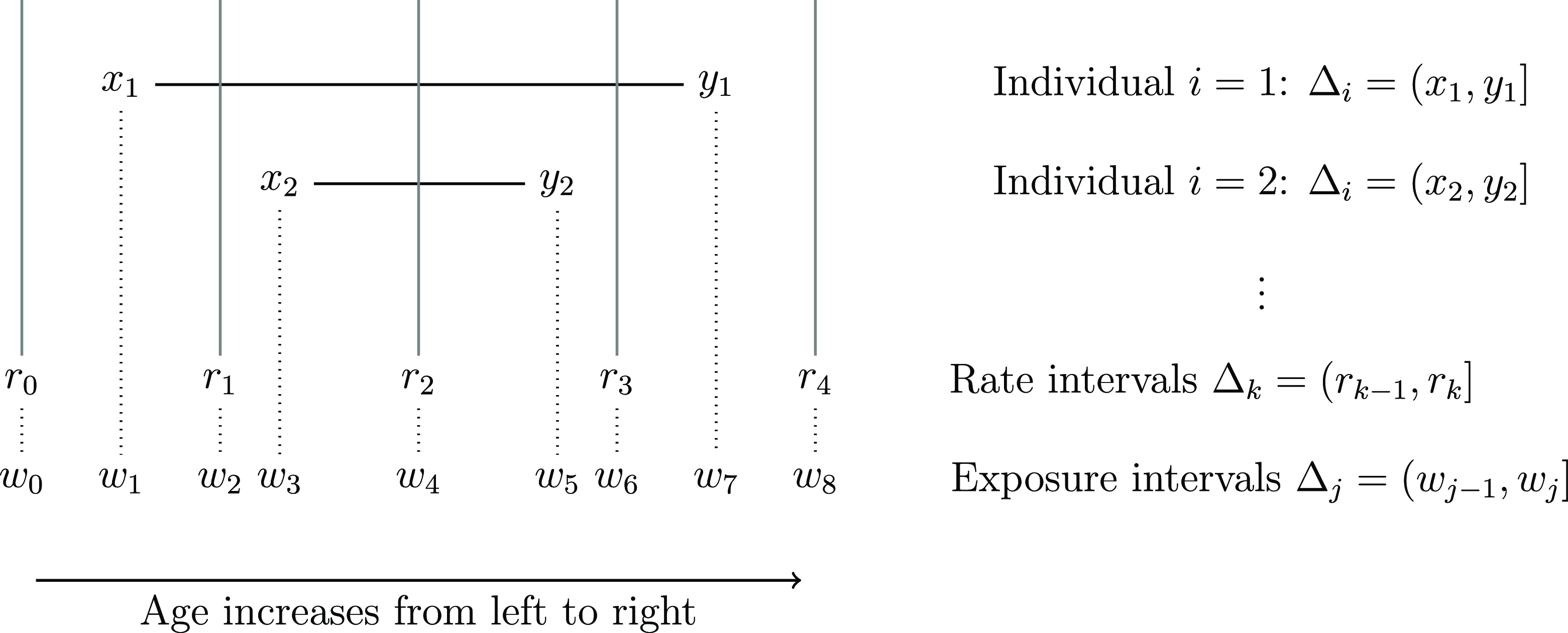
Figure A1. Rate intervals, individual observations and exposure intervals. Rate-interval boundaries, $\left\{ {{r_k}} \right\}$
, are set by the analyst, and here are not necessarily integers, nor evenly spaced. The data are paired ages of the start and end of individual observations,
$\left\{ {{r_k}} \right\}$
, are set by the analyst, and here are not necessarily integers, nor evenly spaced. The data are paired ages of the start and end of individual observations, $\left( {{x_i},{y_i}} \right)$
. The set of exposure interval boundaries,
$\left( {{x_i},{y_i}} \right)$
. The set of exposure interval boundaries, $\left\{ {{w_j}} \right\}$
, is defined as the ordered union of
$\left\{ {{w_j}} \right\}$
, is defined as the ordered union of $\left\{ {{r_k}} \right\}$
,
$\left\{ {{r_k}} \right\}$
, $\left\{ {{x_i}} \right\}$
and
$\left\{ {{x_i}} \right\}$
and $\left\{ {{y_i}} \right\}$
. One consequence is that each exposure interval
$\left\{ {{y_i}} \right\}$
. One consequence is that each exposure interval ${{\rm{\Delta }}_j}$
is always completely contained within a corresponding rate interval
${{\rm{\Delta }}_j}$
is always completely contained within a corresponding rate interval ${{\rm{\Delta }}_k}$
.
${{\rm{\Delta }}_k}$
.
We show equality assuming an arbitrary form of hazard rate ${\mu _x}$
, making no parametric assumptions. This includes as a special case the assumption of piecewise-constant hazard rates, constant on each rate interval, usually made in conjunction with the assumption that total deaths
${\mu _x}$
, making no parametric assumptions. This includes as a special case the assumption of piecewise-constant hazard rates, constant on each rate interval, usually made in conjunction with the assumption that total deaths ${D_x}$
in each rate interval are Poisson random variables.
${D_x}$
in each rate interval are Poisson random variables.
The result here, which resides in the equality of expressions in equations (A5) and (A6), is quite detailed, and follows by selecting elements of three different partitions of the age range in precise ways. This contrasts with Section 4.7, where the same result follows as an easy consequence of the definitions in the counting process representation of the data.
Suppose we have $M$
lives, not all identical, the
$M$
lives, not all identical, the $i$
th individual being observed between ages
$i$
th individual being observed between ages ${x_i}$
and
${x_i}$
and ${x_i} + {v_i}$
and the random variable
${x_i} + {v_i}$
and the random variable ${d_i}$
indicating death or censoring at age
${d_i}$
indicating death or censoring at age ${x_i} + {v_i}$
. Define
${x_i} + {v_i}$
. Define ${y_i} = {x_i} + {v_i}$
, and let
${y_i} = {x_i} + {v_i}$
, and let ${{\rm{\Delta }}_i}$
be the interval
${{\rm{\Delta }}_i}$
be the interval $\left( {{x_i},{y_i}} \right]$
on which the
$\left( {{x_i},{y_i}} \right]$
on which the $i$
th individual is observed.
$i$
th individual is observed.
We wish to introduce a set of rate intervals and write down contributions to the likelihood for the $i$
th individual over those rate intervals that intersect
$i$
th individual over those rate intervals that intersect ${{\rm{\Delta }}_i}$
. We need some detailed definitions, which we introduce in three steps.
${{\rm{\Delta }}_i}$
. We need some detailed definitions, which we introduce in three steps.
Step 1: Intervals: Let the sequence of ages ${r_0} \lt {r_1} \lt \ldots \lt {r_K}$
, with
${r_0} \lt {r_1} \lt \ldots \lt {r_K}$
, with ${r_0} \le {\rm{mi}}{{\rm{n}}_i}{\,}{x_i}$
and
${r_0} \le {\rm{mi}}{{\rm{n}}_i}{\,}{x_i}$
and ${r_K} \ge {\rm{ma}}{{\rm{x}}_i}{\,}{y_i}$
, define the rate intervals
${r_K} \ge {\rm{ma}}{{\rm{x}}_i}{\,}{y_i}$
, define the rate intervals ${{\rm{\Delta }}_k} = \left( {{r_{k - 1}},{r_k}} \right]$ $\left( {k = 1, \ldots, K} \right)$
. Let
$\left( {k = 1, \ldots, K} \right)$
. Let ${w_0} \lt {w_1} \lt \ldots \lt {w_J}$
be the sequence formed by the (ordered) union of the three sequences
${w_0} \lt {w_1} \lt \ldots \lt {w_J}$
be the sequence formed by the (ordered) union of the three sequences ${x_1}, \ldots, {x_M}$
,
${x_1}, \ldots, {x_M}$
, ${y_1}, \ldots, {y_M}$
and
${y_1}, \ldots, {y_M}$
and ${r_0}, \ldots, {r_K}$
and define
${r_0}, \ldots, {r_K}$
and define ${{\rm{\Delta }}_j} = \left( {{w_{j - 1}},{w_j}} \right]$ $\left( {j = 1, \ldots, J} \right)$
. Hence we have rate intervals
$\left( {j = 1, \ldots, J} \right)$
. Hence we have rate intervals ${{\rm{\Delta }}_k}$
, and the
${{\rm{\Delta }}_k}$
, and the $i$
th individual exposed to risk on interval
$i$
th individual exposed to risk on interval ${{\rm{\Delta }}_i}$
, and the intervals
${{\rm{\Delta }}_i}$
, and the intervals ${{\rm{\Delta }}_j}$
are formed from the intersections of all
${{\rm{\Delta }}_j}$
are formed from the intersections of all ${{\rm{\Delta }}_i}$
and
${{\rm{\Delta }}_i}$
and ${{\rm{\Delta }}_k}$
. Figure A1 illustrates these three sequences of intervals.
${{\rm{\Delta }}_k}$
. Figure A1 illustrates these three sequences of intervals.
Step 2: Indicators: For $\left( {j = 1, \ldots, J} \right)$
, define the sequences of indicators:
$\left( {j = 1, \ldots, J} \right)$
, define the sequences of indicators:
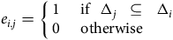 $${e_{i,j}} = \left\{ {\matrix{ 1 \hfill & {{\rm{\;if\;\;}}{{\rm{\Delta }}_j}{\rm{\;\;}} \subseteq {\rm{\;\;}}{{\rm{\Delta }}_i}{\rm{\;}}} \hfill \cr 0 \hfill & {{\rm{\;otherwise\;}}} \hfill \cr } } \right.$$
and:
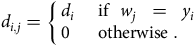 $${d_{i,j}} = \left\{ {\matrix{ {{d_i}} \hfill & {{\rm{\;if\;\;}}{w_j}{\rm{\;\;}} = {\rm{\;\;}}{y_i}{\rm{\;}}} \hfill \cr 0 \hfill & {{\rm{\;otherwise\;}}.} \hfill \cr } } \right.$$
Therefore ${e_{i,j}}$
indicates that the
${e_{i,j}}$
indicates that the $i$
th individual was exposed to risk during
$i$
th individual was exposed to risk during $\left( {{w_{j - 1}},{w_j}} \right]$
, and
$\left( {{w_{j - 1}},{w_j}} \right]$
, and ${d_{i,j}}$
indicates death or censoring of the
${d_{i,j}}$
indicates death or censoring of the $i$
th individual at age
$i$
th individual at age ${w_j}$
.
${w_j}$
.
Step 3: Likelihoods: We can now replace likelihood (13) with the following:
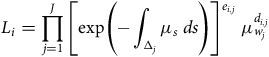 $${L_i} = \mathop \prod \limits_{j = 1}^J {\left[ {{\rm{exp}}\left( { - \mathop \int \nolimits_{{{\rm{\Delta }}_j}} {\mu _s}{\rm{\;}}ds} \right)} \right]^{{e_{i,j}}}}{\rm{\;}}\mu _{{w_j}}^{{d_{i,j}}}$$
and collect together all those intervals ${{\rm{\Delta }}_j}$
that are part of the rate interval
${{\rm{\Delta }}_j}$
that are part of the rate interval ${{\rm{\Delta }}_k}$
:
${{\rm{\Delta }}_k}$
:
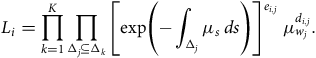 $${L_i} = \mathop \prod \limits_{k = 1}^K \mathop \prod \limits_{{{\rm{\Delta }}_j} \subseteq {{\rm{\Delta }}_k}} {\left[ {{\rm{exp}}\left( { - \mathop \int \nolimits_{{{\rm{\Delta }}_j}} {\mu _s}{\rm{\;}}ds} \right)} \right]^{{e_{i,j}}}}{\rm{\;}}\mu _{{w_j}}^{{d_{i,j}}}.$$
The payoff from all this careful defining of points and intervals comes when we form the total likelihood over all $M$
individuals, denoted by
$M$
individuals, denoted by $L$
:
$L$
:
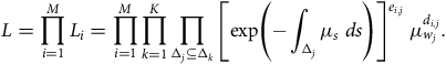 $$L = \mathop \prod \limits_{i = 1}^M {L_i} = \mathop \prod \limits_{i = 1}^M \mathop \prod \limits_{k = 1}^K \mathop \prod \limits_{{{\rm{\Delta }}_j} \subseteq {{\rm{\Delta }}_k}} {\left[ {{\rm{exp}}\left( { - \mathop \int \nolimits_{{{\rm{\Delta }}_j}} {\mu _s}{\rm{\;}}ds} \right)} \right]^{{e_{i,j}}}}{\rm{\;}}\mu _{{w_j}}^{{d_{i,j}}}.$$
Then by reversing the order of the two outer products, we can collect together contributions to each rate interval instead of contributions to each lifetime:
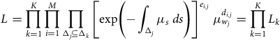 $$L = \mathop \prod \limits_{k = 1}^K \mathop \prod \limits_{i = 1}^M \mathop \prod \limits_{{{\rm{\Delta }}_j} \subseteq {{\rm{\Delta }}_k}} {\left[ {{\rm{exp}}\left( { - \mathop \int \nolimits_{{{\rm{\Delta }}_j}} {\mu _s}{\rm{\;}}ds} \right)} \right]^{{e_{i,j}}}}{\rm{\;}}\mu _{{w_j}}^{{d_{i,j}}} = \mathop \prod \limits_{k = 1}^K {L_k}$$
where we define ${L_k}$
as:
${L_k}$
as:
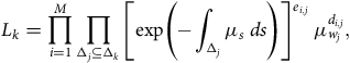 $${L_k} = \mathop \prod \limits_{i = 1}^M \mathop \prod \limits_{{{\rm{\Delta }}_j} \subseteq {{\rm{\Delta }}_k}} {\left[ {{\rm{exp}}\left( { - \mathop \int \nolimits_{{{\rm{\Delta }}_j}} {\mu _s}{\rm{\;}}ds} \right)} \right]^{{e_{i,j}}}}{\rm{\;}}\mu _{{w_j}}^{{d_{i,j}}},$$
which we recognize as the total contribution for rate interval ${{\rm{\Delta }}_k}$
. The desired equality is shown above, namely
${{\rm{\Delta }}_k}$
. The desired equality is shown above, namely $\mathop \prod \nolimits_i {L_i} = \mathop \prod \nolimits_k {L_k}$
. We note that the intricacy of the definitions and the argument (including the presence of two sets of indicators
$\mathop \prod \nolimits_i {L_i} = \mathop \prod \nolimits_k {L_k}$
. We note that the intricacy of the definitions and the argument (including the presence of two sets of indicators ${d_{i,j}}$
and
${d_{i,j}}$
and ${e_{i,j}}$
) stems from the need to handle both points and intervals of time, in different combinations. This need is largely abolished, as far as algebra is concerned, by the definition of the process
${e_{i,j}}$
) stems from the need to handle both points and intervals of time, in different combinations. This need is largely abolished, as far as algebra is concerned, by the definition of the process ${Y^i}\left( x \right)$
in Section 4.3.
${Y^i}\left( x \right)$
in Section 4.3.
Appendix B. The Product-integral
The ordinary integral is familiar to actuaries, the product-integral less so. However, every time an actuary multiplies survival probabilities of the form ${{\rm{\;}}_t}{p_x}$
, she uses a product-integral. It is clear that she uses an ordinary integral, and moreover uses its additive property, since:
${{\rm{\;}}_t}{p_x}$
, she uses a product-integral. It is clear that she uses an ordinary integral, and moreover uses its additive property, since:
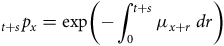 $${{\rm{\;}}_{t + s}}{p_x} = {\rm{exp}}\left( { - \mathop \int \nolimits_0^{t + s} {\mu _{x + r}}{\rm{\;}}dr} \right)$$
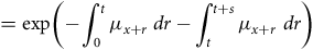 $$ \hskip 79pt= {\rm{exp}}\left( { - \mathop \int \nolimits_0^t {\mu _{x + r}}{\rm{\;}}dr - \mathop \int \nolimits_t^{t + s} {\mu _{x + r}}{\rm{\;}}dr} \right)$$
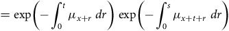 $$ \hskip 108pt= {\rm{exp}}\left( { - \mathop \int \nolimits_0^t {\mu _{x + r}}{\rm{\;}}dr} \right){\rm{\;exp}}\left( { - \mathop \int \nolimits_0^s {\mu _{x + t + r}}{\rm{\;}}dr} \right)$$
 $${ \hskip -25pt= \,_t}{p_x}{{\rm{\;}}_s}{p_{x + t}}.$$
This suggests the exponential function as a link between functions with additive and multiplicative properties, and indeed it is. Start with the following identity, proved in most courses on real analysis (see Hardy (Reference Hardy1992, pp. 410–411)):
 $$\mathop {{\rm{lim}}}\limits_{n \to \infty } {\left( {1 + {1 \over n}} \right)^n} = e.$$
More generally, assuming we may exchange logarithms and limits and then taking just the first-order term of the Taylor expansion ${\rm{log}}\left( {1 + s} \right) = s - {s^2}/2 + {s^3}/3 - \ldots $
(convergent on
${\rm{log}}\left( {1 + s} \right) = s - {s^2}/2 + {s^3}/3 - \ldots $
(convergent on $ - 1 \lt s \le 1$
):
$ - 1 \lt s \le 1$
):
 $${\rm{log}}\mathop {{\rm{lim}}}\limits_{n \to \infty } {\left( {1 + {s \over n}} \right)^n} \approx \mathop {{\rm{lim}}}\limits_{n \to \infty } n{\rm{\;}}{s \over n} = s$$
implying (B2) and more. This is homogeneous, in the sense that $n \times s/n = \mathop \sum \nolimits_1^n s/n$
is a sum of
$n \times s/n = \mathop \sum \nolimits_1^n s/n$
is a sum of $n$
equal summands. Suppose we have a well-behaved function
$n$
equal summands. Suppose we have a well-behaved function $f\left( s \right)$
on an interval
$f\left( s \right)$
on an interval $\left( {a,b} \right]$
. Partition the interval into
$\left( {a,b} \right]$
. Partition the interval into $n$
equal sub-intervals denoted by
$n$
equal sub-intervals denoted by ${{\rm{\Delta }}_1} = \left[ {a,a + h} \right), \ldots, {{\rm{\Delta }}_n} = \left( {b - h,b} \right]$
where
${{\rm{\Delta }}_1} = \left[ {a,a + h} \right), \ldots, {{\rm{\Delta }}_n} = \left( {b - h,b} \right]$
where $h = \left( {b - a} \right)/n$
, and let
$h = \left( {b - a} \right)/n$
, and let $f\left( {{s_k}} \right)$
be the function value at an arbitrarily chosen
$f\left( {{s_k}} \right)$
be the function value at an arbitrarily chosen ${s_k} \in {{\rm{\Delta }}_k}$
(
${s_k} \in {{\rm{\Delta }}_k}$
( $k = 1,2, \ldots, n$
). Then by the same reasoning:
$k = 1,2, \ldots, n$
). Then by the same reasoning:
 $${\rm{log}}\mathop {{\rm{lim}}}\limits_{n \to \infty } \mathop \prod \limits_{k = 1}^n \left( {1 + f\left( {{s_k}} \right){\rm{\,}}h} \right) \approx \mathop {{\rm{lim}}}\limits_{n \to \infty } \mathop \sum \limits_{k = 1}^n f\left( {{s_k}} \right){\rm{\,}}h = \mathop \int \nolimits_a^b f\left( s \right){\rm{\,}}ds.$$
It only remains to replace the interval length $h$
with the more general
$h$
with the more general $ds$
in the limit and exponentiate both sides, giving us the important representation:
$ds$
in the limit and exponentiate both sides, giving us the important representation:
 $$\mathop \prod \limits_{s \in \left( {a,b} \right]} \left( {1 + f\left( s \right){\rm{\,}}ds} \right) = {\rm{exp}}\left( {\mathop \int \nolimits_a^b f\left( s \right){\rm{\,}}ds} \right).$$
Choose the function $f\left( s \right) = - {\mu _{x + s}}$
on the interval
$f\left( s \right) = - {\mu _{x + s}}$
on the interval $\left( {0,t} \right]$
as in a survival probability, and we have the product-integral representation of the familiar identity:
$\left( {0,t} \right]$
as in a survival probability, and we have the product-integral representation of the familiar identity:
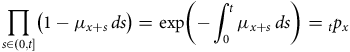 $$\mathop \prod \limits_{s \in \left( {0,t} \right]} \left( {1 - {\mu _{x + s}}{\rm{\,}}ds} \right) = {\rm{exp}}\left( { - \mathop \int \nolimits_0^t {\mu _{x + s}}{\rm{\,}}ds} \right) = {_t}{p_x}$$
which is equation (24).
The above is intuitive and heuristic; for a rigorous account see Gill and Johansen (Reference Gill and Johansen1990) and references therein.


 Open access