


1 Introduction
We will study the following space–time fractional equation:
 $$ \begin{align} \left\{\begin{aligned} &\partial^{\beta}_{t}u(t,x)=-\nu(-\Delta)^{\alpha/2}u(t,x)+f(t,x),\quad (t,x)\in\mathbb R^{1+n}_{+}:=[0,\infty)\times\mathbb R^{n},\\ &u(0,x)=\varphi(x),\ x\in\mathbb R^{n}, \end{aligned} \right. \end{align} $$
with the initial condition $\varphi (\cdot )$
and the nonhomogeneous term
$\varphi (\cdot )$
and the nonhomogeneous term $f(\cdot ,\cdot )$
. Here,
$f(\cdot ,\cdot )$
. Here, $(-\Delta )^{\alpha /2}$
denotes the fractional Laplacian, and the symbol
$(-\Delta )^{\alpha /2}$
denotes the fractional Laplacian, and the symbol $\partial ^{\beta }_{t}$
denotes the Caputo fractional derivative defined as
$\partial ^{\beta }_{t}$
denotes the Caputo fractional derivative defined as
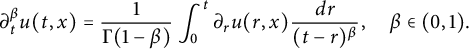 $$ \begin{align*} \partial^{\beta}_{t}u(t,x)=\frac{1}{\Gamma(1-\beta)}\int^{t}_{0}\partial_{r}u(r,x)\frac{dr}{(t-r)^{\beta}},\quad \beta\in(0,1). \end{align*} $$
When $\beta =1$
and
$\beta =1$
and $\alpha =2,$
(1.1) is the classical heat equation, which is extremely important in many areas of mathematics, physics, fluid dynamics, and engineering. When
$\alpha =2,$
(1.1) is the classical heat equation, which is extremely important in many areas of mathematics, physics, fluid dynamics, and engineering. When ${\beta =1}$
and
${\beta =1}$
and $\alpha \in (0,2),$
(1.1) reduces to the space-fractional heat equation, which has been applied to the research of fluid dynamics (see [Reference Constantin and Wu18, Reference Li and Zhai48, Reference Miao, Yuan and Zhang52, Reference Tran, Yu and Zhai60, Reference Wang and Xiao62] and the references therein). When
$\alpha \in (0,2),$
(1.1) reduces to the space-fractional heat equation, which has been applied to the research of fluid dynamics (see [Reference Constantin and Wu18, Reference Li and Zhai48, Reference Miao, Yuan and Zhang52, Reference Tran, Yu and Zhai60, Reference Wang and Xiao62] and the references therein). When $\beta \in (0,1)$
and
$\beta \in (0,1)$
and $\alpha =2,$
(1.1) becomes the time-fractional heat equation
$\alpha =2,$
(1.1) becomes the time-fractional heat equation
 $$ \begin{align} \partial_{t}^{\beta}u(t,x)-\Delta u(t,x)=0, \end{align} $$
which exhibits the subdiffusive behavior and is related with anomalous diffusion, or diffusion in nonhomogeneous media, with random fractal structures (cf. [Reference Meerschaert, Nane and Xiao51]).
The time–space fractional dissipative operator
 $$ \begin{align*} L_{\alpha,\beta}:=\partial^{\beta}_{t}+\nu(-\Delta)^{\alpha},\quad \alpha>0\ \&\ \beta\in(0,1), \end{align*} $$
has the salient significance and backgrounds in mathematical physics. The fractional Laplacian $(-\Delta )^{\alpha }$
plays a significant role in many areas of mathematics, such as harmonic analysis and PDEs. In addition, the fractional Laplacian has been applied to study a wide class of physical systems and engineering problems, including Lévy flights, stochastic interfaces, and anomalous diffusion problems. For example, in fluid mechanics,
$(-\Delta )^{\alpha }$
plays a significant role in many areas of mathematics, such as harmonic analysis and PDEs. In addition, the fractional Laplacian has been applied to study a wide class of physical systems and engineering problems, including Lévy flights, stochastic interfaces, and anomalous diffusion problems. For example, in fluid mechanics, $(-\Delta )^{\alpha }$
is often applied to describe many complicated phenomena via partial differential equations. Caffarelli and Silvestre showed in [Reference Caffarelli and Silvestre10] that any fractional power of the Laplacian can be determined as an operator that maps a Dirichlet boundary condition to a Neumann-type condition via an extension problem. This characterization of
$(-\Delta )^{\alpha }$
is often applied to describe many complicated phenomena via partial differential equations. Caffarelli and Silvestre showed in [Reference Caffarelli and Silvestre10] that any fractional power of the Laplacian can be determined as an operator that maps a Dirichlet boundary condition to a Neumann-type condition via an extension problem. This characterization of $(-\Delta )^{\alpha }$
via the local (degenerate) PDE was first used in [Reference Caffarelli, Salsa and Silvestre9] to get regularity estimates of the obstacle problem for the fractional Laplacian. We also refer the reader to [Reference Caffarelli and Stinga11, Reference Caffarelli and Vasseur12, Reference Herrmann34, Reference Ros-Oton and Serra56] for further information on applications of the fractional Laplacian in PDEs.
$(-\Delta )^{\alpha }$
via the local (degenerate) PDE was first used in [Reference Caffarelli, Salsa and Silvestre9] to get regularity estimates of the obstacle problem for the fractional Laplacian. We also refer the reader to [Reference Caffarelli and Stinga11, Reference Caffarelli and Vasseur12, Reference Herrmann34, Reference Ros-Oton and Serra56] for further information on applications of the fractional Laplacian in PDEs.
The Caputo fractional derivative $\partial ^{\beta }_{t}$
was introduced by Caputo [Reference Caputo13] when studying some anelastic materials and soon became a popular tool in engineering (see also [Reference Bernardis, Martín-Reyes, Stinga and Torrea8, Reference Gorenflo, Luchko and Yamamoto30, Reference Kilbas, Srivastava and Trujillo41, Reference Li and Liu45] for generalizations of Caputo derivatives). Similar to the ordinary derivative
$\partial ^{\beta }_{t}$
was introduced by Caputo [Reference Caputo13] when studying some anelastic materials and soon became a popular tool in engineering (see also [Reference Bernardis, Martín-Reyes, Stinga and Torrea8, Reference Gorenflo, Luchko and Yamamoto30, Reference Kilbas, Srivastava and Trujillo41, Reference Li and Liu45] for generalizations of Caputo derivatives). Similar to the ordinary derivative $\partial _{t}$
, the Caputo derivative is suitable for initial value problems, and is extremely important in physical systems (cf. [Reference Li, Liu and Lu46]) since the derivatives paired with fractional Brownian noise must be Caputo derivatives in physical systems which are different from those in the financial model (see [Reference Dung21]). For this reason, the time-fractional calculus is widely used in a rather large number of scientific branches, such as statistical mechanics, theoretical physics, theoretical neuroscience, the theory of complex chemical reactions, fluid dynamics, hydrology, and mathematical finance (see, e.g., [Reference Khoshnevisan40] for an extensive list of references).
$\partial _{t}$
, the Caputo derivative is suitable for initial value problems, and is extremely important in physical systems (cf. [Reference Li, Liu and Lu46]) since the derivatives paired with fractional Brownian noise must be Caputo derivatives in physical systems which are different from those in the financial model (see [Reference Dung21]). For this reason, the time-fractional calculus is widely used in a rather large number of scientific branches, such as statistical mechanics, theoretical physics, theoretical neuroscience, the theory of complex chemical reactions, fluid dynamics, hydrology, and mathematical finance (see, e.g., [Reference Khoshnevisan40] for an extensive list of references).
In recent years, fractional partial differential equations with Caputo time derivatives have attracted the attention of many researchers. There exist many related results on this topic. In [Reference Allen, Caffarelli and Vasseur6], Allen et al. established a De Giorgi–Nash–Moser Hölder regularity theorem for solutions and also proved results regarding the existence, the uniqueness, and higher regularities in time. Eidelman and Kochubei in [Reference Eidelman and Kochubei22] provided fundamental solutions of the Cauchy problem of fractional diffusion equations. Chen et al. [Reference Chen, Kim and Kim17] proved the existence and uniqueness of solutions to a class of SPDEs with time-fractional derivatives. Li and Liu in [Reference Li and Liu44] developed some compactness criteria that are analogies of the Aubin–Lions lemma for the existence of weak solutions to time-fractional PDEs. In [Reference Allen5], Allen proved the uniqueness for weak solutions to abstract parabolic equations with fractional Caputo or Marchaud time derivatives. Interested readers can also refer to [Reference Dung21, Reference El-Borai23, Reference Feng, Li, Liu and Xu24, Reference Ford, Xiao and Yan26, Reference Galeone and Garrappa27, Reference Gorenflo, Mainardi, Moretti and Paradisi31, Reference Hairer32, Reference Nualart and Ouknine55, Reference Sakthivel, Suganya and Anthoni57, Reference Taylor59, Reference Wang and Zhou61].
Compared with the aforesaid achievements, the study of space–time fractional PDEs with the Caputo time derivative and the fractional Laplacian on spatial variables is relatively few. In [Reference Kolokoltsov and Veretennikova42], Kolokoltsov and Veretennikova studied the Cauchy problem for nonlinear in time and space pseudo-differential equations and analyzed the well-posedness and smoothing properties of the corresponding linear equation. For a nonlocal heat equation with fractional order both in space and time, Kemppainen et al. [Reference Kemppainen, Siljander and Zacher39] proved a representation formula for classical solutions, a quantitative decay rate at which the solution tends to the fundamental solution, an optimal $L^2$
-decay of mild solutions in all dimensions, and
$L^2$
-decay of mild solutions in all dimensions, and $L^2$
-decay of weak solutions via energy methods. For a system of nonlinear space–time fractional SPDEs, Mijena and Nane in [Reference Mijena and Nane53] proved the existence and the uniqueness of the mild solution, and the bounds for intermittency fronts solutions to these equations were investigated in [Reference Mijena and Nane54]. For space–time fractional SPDEs in a Gaussian noisy environment, Chen et al. in [Reference Chen, Hu, Hu and Huang16] proved the existence and the uniqueness of solutions. Foondun and Nane [Reference Foondun and Nane25] studied the asymptotic properties of space–time fractional SPDEs. Time-fractional Hamilton–Jacobi equations and the notion of viscosity solutions have been discussed in [Reference Giga and Namba28, Reference Kolokoltsov and Veretennikova43].
$L^2$
-decay of weak solutions via energy methods. For a system of nonlinear space–time fractional SPDEs, Mijena and Nane in [Reference Mijena and Nane53] proved the existence and the uniqueness of the mild solution, and the bounds for intermittency fronts solutions to these equations were investigated in [Reference Mijena and Nane54]. For space–time fractional SPDEs in a Gaussian noisy environment, Chen et al. in [Reference Chen, Hu, Hu and Huang16] proved the existence and the uniqueness of solutions. Foondun and Nane [Reference Foondun and Nane25] studied the asymptotic properties of space–time fractional SPDEs. Time-fractional Hamilton–Jacobi equations and the notion of viscosity solutions have been discussed in [Reference Giga and Namba28, Reference Kolokoltsov and Veretennikova43].
Different from the abovementioned works on space–time fractional equations, in this paper, we aim to investigate the regularity properties and the blow-up set of solutions to equation (1.1) via capacities. This work is closely motivated by [Reference Chang and Xiao15, Reference Jiang, Xiao, Yang and Zhai35, Reference Johnson36, Reference Xiao64, Reference Xiao65]. Using the fractional Duhamel principle, the mild solution of (1.1) is represented as
 $$ \begin{align*} u(t,x)=\int_{\mathbb R^{n}}G_{t}(x-y)\varphi(y)dy+\int^{t}_{0}\int_{\mathbb R^{n}}G_{t-s}(x-y)\partial^{1-\beta}_{s}f(s,y)dyds. \end{align*} $$
Let $f(t,x)=I^{1-\beta }_{t}g(t,x)$
, where
$f(t,x)=I^{1-\beta }_{t}g(t,x)$
, where $I^{1-\beta }_{t}$
denotes the fractional integral corresponding to the time variable t. Then
$I^{1-\beta }_{t}$
denotes the fractional integral corresponding to the time variable t. Then
 $$ \begin{align} u(t,x)=\int_{\mathbb R^{n}}G_{t}(x-y)\varphi(y)dy+\int^{t}_{0}\int_{\mathbb R^{n}}G_{t-s}(x-y)g(s,y)dyds. \end{align} $$
Set
 $$ \begin{align*}\left\{\begin{aligned} R_{\alpha,\beta}(\varphi)(t,x)&:=\int_{\mathbb R^{n}}G_{t}(x-y)\varphi(y)dy,\\ G_{\alpha,\beta}(g)(t,x)&:=\int^{t}_{0}\int_{\mathbb R^{n}}G_{t-s}(x-y)g(s,y)dyds. \end{aligned}\right.\end{align*} $$
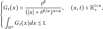
Under the assumption that $\alpha>n$
and
$\alpha>n$
and $\beta \in (0,1)$
, we first establish the homogeneous and inhomogeneous Strichartz-type estimates for (1.1), some other space–time estimates of
$\beta \in (0,1)$
, we first establish the homogeneous and inhomogeneous Strichartz-type estimates for (1.1), some other space–time estimates of $G_{\alpha ,\beta }(g)$
, and the regularity of
$G_{\alpha ,\beta }(g)$
, and the regularity of $R_{\alpha ,\beta }(\varphi )$
and
$R_{\alpha ,\beta }(\varphi )$
and $G_{\alpha ,\beta }(g),$
respectively. Strichartz-type estimates are significant tools for PDEs, such as nonlinear wave equations and Schrödinger equations (see [Reference Ginibre and Velo29, Reference Kato37, Reference Keel and Tao38, Reference Miao, Yuan and Zhang52, Reference Staffilani and Tataru58, Reference Zhai66]). In [Reference Foondun and Nane25], Foondun and Nane proved that the space–time fractional heat kernel
$G_{\alpha ,\beta }(g),$
respectively. Strichartz-type estimates are significant tools for PDEs, such as nonlinear wave equations and Schrödinger equations (see [Reference Ginibre and Velo29, Reference Kato37, Reference Keel and Tao38, Reference Miao, Yuan and Zhang52, Reference Staffilani and Tataru58, Reference Zhai66]). In [Reference Foondun and Nane25], Foondun and Nane proved that the space–time fractional heat kernel $G_{t}(\cdot )$
satisfies the following estimate:
$G_{t}(\cdot )$
satisfies the following estimate:
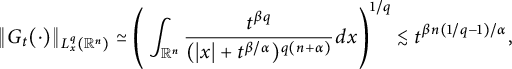
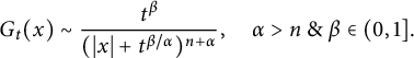 $$ \begin{align} G_{t}(x)\sim \frac{t^{\beta}}{(|x|+t^{\beta/\alpha})^{n+\alpha}},\quad \alpha>n\ \&\ \beta\in(0,1]. \end{align} $$
It follows from (1.4) and the Young inequality that
 $$ \begin{align} \|R_{\alpha,\beta}(\varphi)\|_{L^{p}_{x}(\mathbb R^{n})}\lesssim t^{-n\beta(1/r-1/p)/\alpha}\|\varphi\|_{L^{r}_{x}(\mathbb R^{n})},\quad 1\leq r\leq p\leq\infty. \end{align} $$
Inequality (1.5) allows us, in Section 2.2, to deduce the Strichartz-type estimates and the space–time estimates for $R_{\alpha ,\beta }$
and
$R_{\alpha ,\beta }$
and $G_{\alpha ,\beta }$
related to
$G_{\alpha ,\beta }$
related to $L^{q}_{t}(I; L^{p}_{x}(\mathbb R^{n}))$
, respectively. Here, the mixed norm Lebesgue space
$L^{q}_{t}(I; L^{p}_{x}(\mathbb R^{n}))$
, respectively. Here, the mixed norm Lebesgue space $L^{q}_{t}(I; L^{p}_{x}(\mathbb R^{n}))$
,
$L^{q}_{t}(I; L^{p}_{x}(\mathbb R^{n}))$
, $1\leq p,q\leq \infty ,$
is defined as the set of all measurable functions
$1\leq p,q\leq \infty ,$
is defined as the set of all measurable functions $g(\cdot ,\cdot )$
over an interval
$g(\cdot ,\cdot )$
over an interval $I\subseteq (0,\infty )$
satisfying
$I\subseteq (0,\infty )$
satisfying
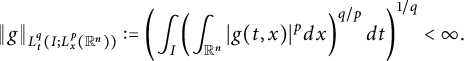 $$ \begin{align*} \|g\|_{L^{q}_{t}(I; L^{p}_{x}(\mathbb R^{n}))}:=\left(\int_{I}\left(\int_{\mathbb R^{n}}|g(t,x)|^{p}dx\right)^{q/p}dt\right)^{1/q}<\infty. \end{align*} $$
Specially, for $I=(0,\infty )$
, we denote
$I=(0,\infty )$
, we denote $L^{q}_{t}((0,\infty ); L^{p}_{x}(\mathbb R^{n}))$
by
$L^{q}_{t}((0,\infty ); L^{p}_{x}(\mathbb R^{n}))$
by $L^{q}_{t}L^{p}_{x}(\mathbb R^{1+n}_{+}).$
These space–time estimates obtained in Section 2.2 will be used to compute the lower bound of the capacities of fractional parabolic balls. Moreover, we investigate the regularities of
$L^{q}_{t}L^{p}_{x}(\mathbb R^{1+n}_{+}).$
These space–time estimates obtained in Section 2.2 will be used to compute the lower bound of the capacities of fractional parabolic balls. Moreover, we investigate the regularities of $R_{\alpha ,\beta }$
and
$R_{\alpha ,\beta }$
and $G_{\alpha ,\beta }$
. By the aid of fractional heat kernels
$G_{\alpha ,\beta }$
. By the aid of fractional heat kernels $K_{\alpha ,t}(\cdot )$
, in Proposition 2.11, we prove that there exist positive constants C and
$K_{\alpha ,t}(\cdot )$
, in Proposition 2.11, we prove that there exist positive constants C and $\delta $
such that for
$\delta $
such that for $|h|<t^{\beta /\alpha }$
,
$|h|<t^{\beta /\alpha }$
,
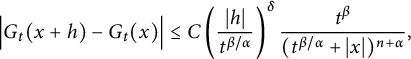 $$ \begin{align*} \Big|G_{t}(x+h)-G_{t}(x)\Big|\leq C\left(\frac{|h|}{t^{\beta/\alpha}}\right)^{\delta}\frac{t^{\beta}}{(t^{\beta/\alpha}+|x|)^{n+\alpha}}, \end{align*} $$
which, together with the estimate
 $$ \begin{align*} &\left|R_{\alpha,\beta}(\varphi)(t_{1},x)-R_{\alpha,\beta}(\varphi)(t_{2},x)\right| \\&\quad\lesssim\|\varphi\|_{L^{p}_{x}(\mathbb R^{n})}\left|t_{1}^{\beta(1-1/\alpha-n/\alpha p)}-t_{2}^{\beta(1-1/\alpha-n/\alpha p)}\right|,\quad 1\leq p\leq \infty, \end{align*} $$
implies that $R_{\alpha ,\beta }(\varphi )$
is continuous on
$R_{\alpha ,\beta }(\varphi )$
is continuous on $\mathbb R^{1+n}_{+}$
for
$\mathbb R^{1+n}_{+}$
for $\varphi \in L^{p}_{x}(\mathbb R^{n})$
(see Theorem 2.12). Let
$\varphi \in L^{p}_{x}(\mathbb R^{n})$
(see Theorem 2.12). Let $p\in [1,\infty )$
,
$p\in [1,\infty )$
, $1<q<\infty $
,
$1<q<\infty $
, $n\beta /p+\alpha /q<\alpha $
,
$n\beta /p+\alpha /q<\alpha $
, $(t,x)\in \mathbb R^{1+n}_{+}$
, and
$(t,x)\in \mathbb R^{1+n}_{+}$
, and $\|g\|_{L^{q}_{t}L^{p}_{x}(\mathbb R^{1+n}_{+})}<\infty $
. For the inhomogeneous part
$\|g\|_{L^{q}_{t}L^{p}_{x}(\mathbb R^{1+n}_{+})}<\infty $
. For the inhomogeneous part $G_{\alpha ,\beta }$
, under the assumption that
$G_{\alpha ,\beta }$
, under the assumption that $(t,x)$
is sufficiently close to
$(t,x)$
is sufficiently close to $(t_{0}, x_{0})$
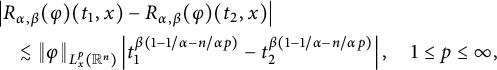
, the following Hölder continuity holds, precisely:
$(t_{0}, x_{0})$
, the following Hölder continuity holds, precisely:
 $$ \begin{align*} &\left|G_{\alpha,\beta}(g)(t,x)-G_{\alpha,\beta}(g)(t_{0}, x_{0})\right|\\&\quad\lesssim \|g\|_{L^{q}_{t}L^{p}_{x}(\mathbb R^{1+n}_{+})}\left(|t-t_{0}|^{1-1/q-\beta n/p\alpha} +|x-x_{0}|^{\alpha(1-1/q)/\beta-n/p}\right) \end{align*} $$
(see Theorem 2.13).
Theorems 2.12 and 2.13 indicate that the blow-up phenomenon of mild solutions to (1.1) merely occurs on the nonlinear part of (1.3), i.e., $G_{\alpha ,\beta }(g)$
for
$G_{\alpha ,\beta }(g)$
for $n\beta /p+\alpha /q>\alpha $
. Based on this observation, in Section 3, we introduce the following blow-up set, denoted by
$n\beta /p+\alpha /q>\alpha $
. Based on this observation, in Section 3, we introduce the following blow-up set, denoted by $\mathcal {B}[G_{\alpha ,\beta }(g), p,q]$
, of solutions to equation (1.1):
$\mathcal {B}[G_{\alpha ,\beta }(g), p,q]$
, of solutions to equation (1.1):
 $$ \begin{align*} \mathcal{B}[G_{\alpha,\beta}(g), p,q]:=\left\{(t,x)\in\mathbb R^{1+n}_{+}:\ G_{\alpha,\beta}(g)(t,x)=\infty\right\} \end{align*} $$
for nonnegative functions $g(\cdot ,\cdot )\in L^{q}_{t}L^{p}_{x}(\mathbb R^{1+n}_{+})$
. We apply capacities to measure the size, i.e., the Hausdorff dimension, of
$g(\cdot ,\cdot )\in L^{q}_{t}L^{p}_{x}(\mathbb R^{1+n}_{+})$
. We apply capacities to measure the size, i.e., the Hausdorff dimension, of $\mathcal {B}[G_{\alpha ,\beta }(g), p,q]$
. In the literature, capacities related to operators and given function spaces are widely applied in the research of the potential theory and partial differential equations. For example, the Besov-type capacities
$\mathcal {B}[G_{\alpha ,\beta }(g), p,q]$
. In the literature, capacities related to operators and given function spaces are widely applied in the research of the potential theory and partial differential equations. For example, the Besov-type capacities $cap(\cdot; \dot {\Lambda }^{p,q}_{\alpha })$
were used to establish the embedding of homogeneous Besov spaces into Lorentz spaces with respect to nonnegative Borel measures (see [Reference Adams and Xiao4, Reference Maz’ya50, Reference Wu63, Reference Xiao65]). The embedding of Sobolev spaces via heat equations and the p-variational capacity was due to Xiao [Reference Xiao64, Reference Xiao65]. In [Reference Dafni, Karadzhov and Xiao20], Dafni et al. introduced a class of measures generated by Riesz, or Bessel, or Besov capacities, and established geometric characterizations of these measures. For further information on this topic, we refer the reader to [Reference Adams1, Reference Chang and Xiao15, Reference Costea19, Reference Li, Shi, Hu and Zhai47, Reference Zhai67] and the references therein.
$cap(\cdot; \dot {\Lambda }^{p,q}_{\alpha })$
were used to establish the embedding of homogeneous Besov spaces into Lorentz spaces with respect to nonnegative Borel measures (see [Reference Adams and Xiao4, Reference Maz’ya50, Reference Wu63, Reference Xiao65]). The embedding of Sobolev spaces via heat equations and the p-variational capacity was due to Xiao [Reference Xiao64, Reference Xiao65]. In [Reference Dafni, Karadzhov and Xiao20], Dafni et al. introduced a class of measures generated by Riesz, or Bessel, or Besov capacities, and established geometric characterizations of these measures. For further information on this topic, we refer the reader to [Reference Adams1, Reference Chang and Xiao15, Reference Costea19, Reference Li, Shi, Hu and Zhai47, Reference Zhai67] and the references therein.
To measure the Hausdorff dimension of the blow-up set of the wave equation, in [Reference Adams2], Adams introduced a class of capacities related to the wave operator $\square $
and
$\square $
and $L^{q}_{t}L^{p}_{x}$
-norm spaces, and studied the size (in terms of Hausdorff content) of the blow-up sets of weak solutions to the nonhomogeneous wave equation in three space dimensions. By a similar idea, Jiang et al. [Reference Jiang, Xiao, Yang and Zhai35] applied the
$L^{q}_{t}L^{p}_{x}$
-norm spaces, and studied the size (in terms of Hausdorff content) of the blow-up sets of weak solutions to the nonhomogeneous wave equation in three space dimensions. By a similar idea, Jiang et al. [Reference Jiang, Xiao, Yang and Zhai35] applied the $L^{q}_{t}L^{p}_{x}$
-type capacities to investigate the blow-up set of a weak solution to the special case
$L^{q}_{t}L^{p}_{x}$
-type capacities to investigate the blow-up set of a weak solution to the special case $\beta =1$
of equation (1.1). Following the idea of [Reference Adams2, Reference Jiang, Xiao, Yang and Zhai35], we introduce the following
$\beta =1$
of equation (1.1). Following the idea of [Reference Adams2, Reference Jiang, Xiao, Yang and Zhai35], we introduce the following $L^{q}_{t}L^p_{x}$
-capacity associated with
$L^{q}_{t}L^p_{x}$
-capacity associated with $G_{\alpha ,\beta }.$
Definition 1.1 Let $1\leq p,q<\infty $
. Denote by
$1\leq p,q<\infty $
. Denote by $p\wedge q:=\min \{p,q\}$
. For any set
$p\wedge q:=\min \{p,q\}$
. For any set $E\subset \mathbb R^{n+1}_{+}$
, define
$E\subset \mathbb R^{n+1}_{+}$
, define
 $$ \begin{align*} C^{(\alpha,\beta)}_{p,q}(E):=\inf\Big\{\|g\|^{p\wedge q}_{L^{q}_{t}L^{p}_{x}(\mathbb R^{1+n}_{+})}:\ g\geq 0\ \&\ G_{\alpha,\beta}(g)\geq 1_{E}\Big\} \end{align*} $$
be the $L^{q}_{t}L^{p}_{x}$
-capacity of E for the space–time fractional dissipative operator, where
$L^{q}_{t}L^{p}_{x}$
-capacity of E for the space–time fractional dissipative operator, where $1_{E}$
is the characteristic function of E.
$1_{E}$
is the characteristic function of E.
In Sections 3.1–3.3, we study the dual form, the basic properties of the $L^{q}_{t}L^p_{x}$
-capacity
$L^{q}_{t}L^p_{x}$
-capacity $C^{(\alpha ,\beta )}_{p,q}(\cdot )$
, and further, utilize Theorem 2.6 to estimate the
$C^{(\alpha ,\beta )}_{p,q}(\cdot )$
, and further, utilize Theorem 2.6 to estimate the $L^{q}_{t}L^p_{x}$
-capacities of fractional parabolic balls
$L^{q}_{t}L^p_{x}$
-capacities of fractional parabolic balls $B^{(\alpha ,\beta )}_{r_{0}}(t_{0},x_{0})$
. In Section 3.4, denote by
$B^{(\alpha ,\beta )}_{r_{0}}(t_{0},x_{0})$
. In Section 3.4, denote by $E_{\lambda }$
with
$E_{\lambda }$
with $ \lambda>0,$
the distribution set of
$ \lambda>0,$
the distribution set of $G_{\alpha ,\beta }$
, i.e.,
$G_{\alpha ,\beta }$
, i.e.,
 $$ \begin{align*} E_{\lambda}:=\left\{(t,x)\in\mathbb R^{1+n}_{+}:\quad G_{\alpha,\beta}(g)(t,x)>\lambda\right\}. \end{align*} $$
Let $1\leq p,q<\infty $
,
$1\leq p,q<\infty $
, $\alpha>n$
and
$\alpha>n$
and $\beta \in (0,1)$
. We obtain the following capacitary strong-type inequality:
$\beta \in (0,1)$
. We obtain the following capacitary strong-type inequality:
 $$ \begin{align*} \int^{\infty}_{0}\lambda^{p\wedge q}C^{(\alpha,\beta)}_{p,q}(E_{\lambda})\frac{d\lambda}{\lambda}\lesssim \|g\|^{p\wedge q}_{L^{q}_{t}L^{p}_{x}(\mathbb R^{1+n}_{+})}\quad \forall\ g(\cdot,\cdot)\in L^{q}_{t}L^{p}_{x}(\mathbb R^{1+n}_{+}) \end{align*} $$
(see Theorem 3.8). As a corollary of Theorem 3.8, in Theorem 3.10, we deduce an equivalent condition of the embedding from $L^{q}_{t}L^{p}_{x}(\mathbb R^{1+n}_{+})$
to Lorentz spaces
$L^{q}_{t}L^{p}_{x}(\mathbb R^{1+n}_{+})$
to Lorentz spaces $L^{(r,s)}(\mathbb R^{1+n}_{+},\mu )$
. By use of the results obtained in Sections 3.2 and 3.3, we obtain that the Hausdorff dimension of
$L^{(r,s)}(\mathbb R^{1+n}_{+},\mu )$
. By use of the results obtained in Sections 3.2 and 3.3, we obtain that the Hausdorff dimension of $\mathcal {B}[G_{\alpha ,\beta }(g), p,q]$
is dominated by
$\mathcal {B}[G_{\alpha ,\beta }(g), p,q]$
is dominated by $n\beta -\alpha (p\wedge q-1)$
under the assumption that
$n\beta -\alpha (p\wedge q-1)$
under the assumption that $1\leq p<\infty $
and
$1\leq p<\infty $
and $1<q<\infty $
with
$1<q<\infty $
with $\alpha>n$
and
$\alpha>n$
and $(p\wedge q)(n\beta /p+\alpha /q-\alpha )>0$
(see Theorem 4.2).
$(p\wedge q)(n\beta /p+\alpha /q-\alpha )>0$
(see Theorem 4.2).
Remark 1.2
-
(i) In the main results of this paper, we restrict the scope of the index $(\alpha ,\beta )$
to
$(n,\infty )\times (0,1)$
. For equation (1.1), there are many important cases concerning
$\alpha \leq n$
. However, for the characterization of (1.1) via the capacity, we need the convolution kernel
$G_{t}(\cdot )$
satisfies the upper bound estimate:
$$ \begin{align*} G_{t}(x)\leq \frac{Ct^{\beta}}{(|x|+t^{\beta/\alpha})^{n+\alpha}}, \end{align*} $$
$(\alpha ,\beta )$
to
$(n,\infty )\times (0,1)$
. For equation (1.1), there are many important cases concerning
$\alpha \leq n$
. However, for the characterization of (1.1) via the capacity, we need the convolution kernel
$G_{t}(\cdot )$
satisfies the upper bound estimate:
$$ \begin{align*} G_{t}(x)\leq \frac{Ct^{\beta}}{(|x|+t^{\beta/\alpha})^{n+\alpha}}, \end{align*} $$
which is true for
$\alpha>n$
. -
(ii) The results in the paper are stated for assumptions on
$g(\cdot ,\cdot )\in L^{q}_{t}L^{p}_{x}(\mathbb R^{n+1}_{+})$
. In fact, we can replace this assumption by the assumption that the nonhomogeneous term
$f(\cdot ,\cdot )$
satisfies
$$ \begin{align*} \left(\int_{0}^{\infty}\left(\int_{\mathbb R^{n}}|\partial_{t}^{1-\beta}f(t,x)|^{p}dx\right)^{q/p}dt\right)^{1/q}<\infty, \end{align*} $$
which indicates
$g(\cdot ,\cdot )\in L^{q}_{t}L^{p}_{x}(\mathbb R^{n+1}_{+})$
.


Some notations:
-
• Let
$\Omega \subseteq \mathbb R^{n}$
. Throughout this article, we use
${C}(\Omega )$
to denote the space of all continuous functions on
$\Omega $
. Let
$k\in \mathbb {N}_{+}\cup \{\infty \}$
. The symbol
${C}^{k}(\Omega )$
denotes the class of all functions
$f:\ \Omega \rightarrow \mathbb {R}$
with k continuous partial derivatives. Let
$C^{\infty }_{0}(\Omega )$
stand for all infinitely smooth functions with compact supports in
$\Omega $
. -
• For
$1\leq p\leq \infty $
, denote by
$p'$
the conjugate number of p, i.e.,
$1/p+1/p'=1$
.
${\mathsf U}\simeq {\mathsf V}$
represents that there is a constant
$c>0$
such that
$c^{-1}{\mathsf V}\le {\mathsf U}\le c{\mathsf V}$
whose right inequality is also written as
${\mathsf U}\lesssim {\mathsf V}$
. Similarly, one writes
${\mathsf V}\gtrsim {\mathsf U}$
for
${\mathsf V}\ge c{\mathsf U}$
. -
• For convenience, the positive constant C may change from one line to another and usually depends on the dimension n,
$\alpha $
,
$\beta $
, and other fixed parameters. For
$f\in \mathscr {S}(\mathbb {R}^{n})$
,
$\widehat {f}$
means the Fourier transform of f.


2 Regularity estimates
In this section, we investigate the regularity of solutions to (1.1). We first state some preliminaries which will be used in the sequel. For further information, we refer the reader to [Reference Foondun and Nane25] and the references therein.
2.1 Basic estimates of the space–time fractional heat kernel
Let $X_{t}$
denote a symmetric
$X_{t}$
denote a symmetric $\alpha $
stable process with the density function denoted by
$\alpha $
stable process with the density function denoted by $K_{\alpha /2,t}(\cdot )$
. This is characterized through the Fourier transform, which is given by
$K_{\alpha /2,t}(\cdot )$
. This is characterized through the Fourier transform, which is given by
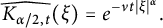 $$ \begin{align*} \widehat{K_{\alpha/2,t}}(\xi)=e^{-\nu t|\xi|^{\alpha}}. \end{align*} $$
Let $D=\{D_{r}, r\geq 0\}$
denote a
$D=\{D_{r}, r\geq 0\}$
denote a $\beta $
-stable subordinator, and let
$\beta $
-stable subordinator, and let $E_{t}$
be its first passage time. It is well known that the density of the time changed
$E_{t}$
be its first passage time. It is well known that the density of the time changed $X_{E_{t}}$
is given by
$X_{E_{t}}$
is given by $G_{t}(x)$
. By conditioning, we have
$G_{t}(x)$
. By conditioning, we have
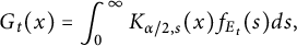 $$ \begin{align} G_{t}(x)=\int^{\infty}_{0}K_{\alpha/2,s}(x)f_{E_{t}}(s)ds, \end{align} $$
where
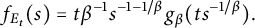 $$ \begin{align*} f_{E_{t}}(s)=t\beta^{-1}s^{-1-1/\beta}g_{\beta}(ts^{-1/\beta}). \end{align*} $$
Here, $g_{\beta }(\cdot )$
is the density function of
$g_{\beta }(\cdot )$
is the density function of $D_{1}$
and is infinitely differentiable on the entire real line, with
$D_{1}$
and is infinitely differentiable on the entire real line, with $g_{\beta }(u)=0$
for
$g_{\beta }(u)=0$
for $u\leq 0$
. Moreover,
$u\leq 0$
. Moreover,
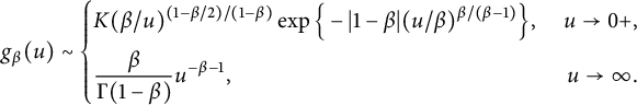 $$ \begin{align}\qquad g_{\beta}(u)\sim\left\{ \begin{aligned} &K(\beta/u)^{(1-\beta/2)/(1-\beta)}\exp\Big\{-|1-\beta|(u/\beta)^{\beta/(\beta-1)}\Big\},\ &u\rightarrow0+,\\ &\frac{\beta}{\Gamma(1-\beta)}u^{-\beta-1},\ &u\rightarrow\infty. \end{aligned}\right. \end{align} $$
Another explicit description of the heat kernel $G_{t}(\cdot )$
is as follows. Denote by
$G_{t}(\cdot )$
is as follows. Denote by $\widetilde {(\cdot )}$
the Laplace transform. Then
$\widetilde {(\cdot )}$
the Laplace transform. Then
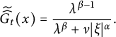 $$ \begin{align*} \widetilde{\widehat{G_{t}}}(x)=\frac{\lambda^{\beta-1}}{\lambda^{\beta}+\nu|\xi|^{\alpha}}. \end{align*} $$
Inverting the Laplace transform yields the Fourier transform of $G_{t}(\cdot )$
is
$G_{t}(\cdot )$
is $\widehat {G_{t}}(\xi )=E_{\beta }(-\nu |\xi |^{\beta }t^{\beta }),$
where
$\widehat {G_{t}}(\xi )=E_{\beta }(-\nu |\xi |^{\beta }t^{\beta }),$
where $E_{\beta }(\cdot )$
is the Mittag–Leffler function, which is defined as
$E_{\beta }(\cdot )$
is the Mittag–Leffler function, which is defined as
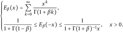 $$ \begin{align*} \left\{\begin{aligned} & E_{\beta}(x)=\sum^{\infty}_{k=0}\frac{x^{k}}{\Gamma(1+\beta k)},\\ &\frac{1}{1+\Gamma(1-\beta)}\leq E_{\beta}(-x)\leq\frac{1}{1+\Gamma(1+\beta)^{-1}x},\quad x>0. \end{aligned}\right. \end{align*} $$
Let $H^{m,n}_{p,q}$
denote the H-function given in [Reference Mathai and Haubold49, Definition 1.9.1, p. 55]. By the formula
$H^{m,n}_{p,q}$
denote the H-function given in [Reference Mathai and Haubold49, Definition 1.9.1, p. 55]. By the formula
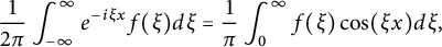 $$ \begin{align*} \frac{1}{2\pi}\int^{\infty}_{-\infty}e^{-i\xi x}f(\xi)d\xi=\frac{1}{\pi}\int^{\infty}_{0}f(\xi)\cos(\xi x)d\xi, \end{align*} $$
it can be deduced from the cosine transform of the H-function (cf. [Reference Haubold, Mathai and Saxena33, equation (12.9)]) that
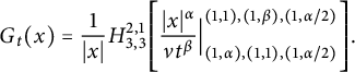 $$ \begin{align*} G_{t}(x)=\frac{1}{|x|}H^{2,1}_{3,3}\Bigg[\frac{|x|^{\alpha}}{\nu t^{\beta}}\Big|^{(1,1),(1,\beta),(1,\alpha/2)}_{(1,\alpha),(1,1),(1,\alpha/2)}\Bigg]. \end{align*} $$
Specially, by reduction formula for the H-function, we can get, for $\alpha =2$
,
$\alpha =2$
,
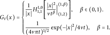 $$ \begin{align*}G_{t}(x)=\left\{\begin{aligned} &\frac{1}{|x|}H^{1,0}_{1,1}\Bigg[\frac{|x|^{2}}{\nu t^{\beta}}\Big|^{(1,\beta)}_{(1,2)}\Bigg],\quad \beta\in (0,1).\\ &\frac{1}{(4\nu\pi t)^{1/2}}\exp(-{|x|^{2}}/{4\nu t}),\quad \beta=1. \end{aligned}\right. \end{align*} $$
Foondun and Nane [Reference Foondun and Nane25] obtained the following estimate for $G_{t}(\cdot )$
.
$G_{t}(\cdot )$
.
Proposition 2.1 [Reference Foondun and Nane25, Lemma 2.1]
Let $\beta \in (0,1)$
.
$\beta \in (0,1)$
.
-
(i) There exists a positive constant
$C_{1}$
such that for all
$x\in \mathbb R^{n}$
, (2.3)
$$ \begin{align} G_{t}(x)\geq C_{1}\min\left\{t^{-\beta n/\alpha},\ \frac{t^{\beta}}{|x|^{n+\alpha}}\right\}. \end{align} $$
-
(ii) If we further suppose that
$\alpha>n$
, then there exists a positive constant
$C_{2}$
such that for all
$x\in \mathbb R^{n}$
, (2.4)
$$ \begin{align} G_{t}(x)\leq C_{2}\min\left\{t^{-\beta n/\alpha},\ \frac{t^{\beta}}{|x|^{n+\alpha}}\right\}. \end{align} $$


The following is an immediate corollary of Proposition 2.1.
Corollary 2.2 Let $\alpha>n$
and
$\alpha>n$
and $\beta \in (0,1)$
. Then
$\beta \in (0,1)$
. Then
 $$ \begin{align} \left\{\begin{aligned} &G_{t}(x)\simeq \frac{t^{\beta}}{(|x|+t^{\beta/\alpha})^{n+\alpha}},\quad (x,t)\in\mathbb R^{1+n}_{+},\\ &\int_{\mathbb R^{n}}G_{t}(x)dx\lesssim 1. \end{aligned}\right. \end{align} $$
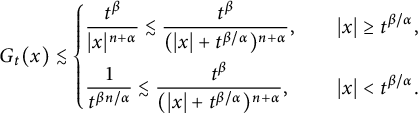
Proof Below, we always assume that $\alpha>n$
. By (i) of Proposition 2.1, it holds
$\alpha>n$
. By (i) of Proposition 2.1, it holds
 $$ \begin{align*} G_{t}(x)\gtrsim\left\{\begin{aligned} &\frac{t^{\beta}}{|x|^{n+\alpha}}\gtrsim \frac{t^{\beta}}{(|x|+t^{\beta/\alpha})^{n+\alpha}},\quad &|x|\geq t^{\beta/\alpha},\\ &\frac{1}{t^{n\beta/\alpha}}\gtrsim\frac{t^{\beta}}{(|x|+t^{\beta/\alpha})^{n+\alpha}},\quad &|x|<t^{\beta/\alpha}. \end{aligned} \right.\end{align*} $$
On the other hand, it can be deduced from (ii) of Proposition 2.1 that
 $$ \begin{align*} G_{t}(x)\lesssim\left\{\begin{aligned} &\frac{t^{\beta}}{|x|^{n+\alpha}}\lesssim \frac{t^{\beta}}{(|x|+t^{\beta/\alpha})^{n+\alpha}},\quad &|x|\geq t^{\beta/\alpha},\\ &\frac{1}{t^{\beta n/\alpha}}\lesssim\frac{t^{\beta}}{(|x|+t^{\beta/\alpha})^{n+\alpha}},\quad &|x|<t^{\beta/\alpha}. \end{aligned}\right.\end{align*} $$
Finally,
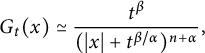 $$ \begin{align*} G_{t}(x)\simeq \frac{t^{\beta}}{(|x|+t^{\beta/\alpha})^{n+\alpha}}, \end{align*} $$
which, via a direct computation, gives
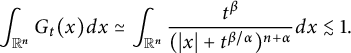 $$ \begin{align*} \int_{\mathbb R^{n}}G_{t}(x)dx \simeq \int_{\mathbb R^{n}}\frac{t^{\beta}}{(|x|+t^{\beta/\alpha})^{n+\alpha}} dx\lesssim 1.\\[-42pt] \end{align*} $$
In the following, we assume $\alpha>n.$
We can deduce the following lemma from Corollary 2.2.
$\alpha>n.$
We can deduce the following lemma from Corollary 2.2.
Lemma 2.3 Let $1\leq r\leq p\leq \infty $
and
$1\leq r\leq p\leq \infty $
and $\varphi \in L^{r}(\mathbb R^{n})$
. For
$\varphi \in L^{r}(\mathbb R^{n})$
. For $\alpha>n$
,
$\alpha>n$
, $\beta \in (0,1)$
, and
$\beta \in (0,1)$
, and $t>0$
,
$t>0$
,
 $$ \begin{align*} \|R_{\alpha,\beta}(\varphi)\|_{L^{p}_{x}(\mathbb R^{n})}\lesssim t^{-n\beta(1/r-1/p)/\alpha}\|\varphi\|_{L^{r}_{x} (\mathbb R^{n})}. \end{align*} $$
Proof Let q obey $1/r+1/q=1/p+1$
. By Young’s inequality,
$1/r+1/q=1/p+1$
. By Young’s inequality,
 $$ \begin{align*} \|R_{\alpha,\beta}(\varphi)\|_{L^{p}_{x}(\mathbb R^{n})} = \|G_{t}\ast\varphi\|_{L^{p}_{x}(\mathbb R^{n})}\lesssim\|\varphi\|_{L^{r}_{x}(\mathbb R^{n})}\|G_{t}(\cdot)\|_{L^{q}_{x}(\mathbb R^{n})}. \end{align*} $$
It follows from Corollary 2.2 that
 $$ \begin{align*} \|G_{t}(\cdot)\|_{L^{q}_{x}(\mathbb R^{n})} \simeq \Bigg(\int_{\mathbb R^{n}}\frac{t^{\beta q}}{(|x|+t^{\beta/\alpha})^{q(n+\alpha)}}dx\Bigg)^{1/q}\lesssim t^{\beta n(1/q-1)/\alpha}, \end{align*} $$
which implies
 $$ \begin{align*} \|R_{\alpha,\beta}(\varphi)\|_{L^{p}_{x}(\mathbb R^{n})} \lesssim t^{\beta n(1/q-1)/\alpha}\|\varphi\|_{L^{r}_{x}(\mathbb R^{n})}=t^{-\beta n(1/r-1/p)/\alpha}\|\varphi\|_{L^{r}_{x}(\mathbb R^{n})}.\\[-35pt] \end{align*} $$
2.2 Strichartz-type estimates
In this section, we establish homogeneous and inhomogeneous Strichartz-type estimates.
Definition 2.4 Let $\mathbb X$
be a Banach space, and let
$\mathbb X$
be a Banach space, and let $I=[0, T)$
.
$I=[0, T)$
.
-
(i) The space
$C_{\sigma }(I, \mathbb X)$
is defined as the set of all
$f\in C(I; \mathbb X)$
such that
$$ \begin{align*} \|f\|_{C_{\sigma}(I; \mathbb X)}:=\sup_{t\in I}t^{1/\sigma}\|f(t,\cdot)\|_{\mathbb X}<\infty. \end{align*} $$
-
(ii) The space
$C_{0}(I; \mathbb X)$
is defined as the set of all bounded continuous functions from I to
$\mathbb X$
.


For $R_{\alpha ,\beta }(\varphi )$
, we can prove the following Strichartz-type estimates.
$R_{\alpha ,\beta }(\varphi )$
, we can prove the following Strichartz-type estimates.
Theorem 2.5 Assume that $\alpha>n$
and
$\alpha>n$
and $0<\beta <1$
. Let
$0<\beta <1$
. Let $1\leq r\leq p<\infty $
satisfying
$1\leq r\leq p<\infty $
satisfying $1/q=\beta n(1/r-1/p)/\alpha $
. Given
$1/q=\beta n(1/r-1/p)/\alpha $
. Given $\varphi \in L^{r}(\mathbb R^{n})$
and
$\varphi \in L^{r}(\mathbb R^{n})$
and $I=[0,T)$
with
$I=[0,T)$
with $0<T\leq \infty $
.
$0<T\leq \infty $
.
-
(i)
$R_{\alpha ,\beta }(\varphi )\in L^{q}_{t}(I; L^{p}_{x}(\mathbb R^{n}))\cap C_{0}(I; L^{r}_{x}(\mathbb R^{n}))$
with the estimate
$$ \begin{align*} \|R_{\alpha,\beta}(\varphi)\|_{L^{q}_{t}(I; L^{p}_{x}(\mathbb R^{n}))}\lesssim \|\varphi\|_{L^{r}_{x}(\mathbb R^{n})}. \end{align*} $$
-
(ii)
$R_{\alpha ,\beta }(\varphi )\in C_{q}(I; L^{p}_{x}(\mathbb R^{n}))\cap C_{0}(I; L^{r}_{x}(\mathbb R^{n}))$
with the estimate
$$ \begin{align*} \|R_{\alpha,\beta}(\varphi)\|_{C_{q}(I; L^{p}_{x}(\mathbb R^{n}))}\lesssim \|\varphi\|_{L^{r}_{x}(\mathbb R^{n})}. \end{align*} $$


Proof (i) We divide the argument into two cases.
Case 1: $p=r$
and
$p=r$
and $q=\infty $
. By Lemma 2.3, we obtain
$q=\infty $
. By Lemma 2.3, we obtain
 $$ \begin{align*} \|R_{\alpha,\beta}(\varphi)\|_{L^{\infty}_{t}(I; L^{r}_{x}(\mathbb R^{n}))} \lesssim \sup_{t>0}t^{-n\beta(1/r-1/r)/\alpha}\|\varphi\|_{L^{r}_{x}(\mathbb R^{n})}\lesssim \|\varphi\|_{L^{r}_{x}(\mathbb R^{n})}. \end{align*} $$
Case 2: $p\neq r$
. Denote
$p\neq r$
. Denote $F(t)(\varphi )=\|R_{\alpha ,\beta }(\varphi )\|_{L^{p}_{x}(\mathbb R^{n})}$
. Since
$F(t)(\varphi )=\|R_{\alpha ,\beta }(\varphi )\|_{L^{p}_{x}(\mathbb R^{n})}$
. Since $1/q=\beta n(1/r-1/p)/\alpha $
, a further use of Lemma 2.3 can deduce that
$1/q=\beta n(1/r-1/p)/\alpha $
, a further use of Lemma 2.3 can deduce that
 $$ \begin{align} \qquad F(t)(\varphi)= \|R_{\alpha,\beta}(\varphi)\|_{L^{p}_{x}(\mathbb R^{n})}\lesssim t^{-n\beta(1/r-1/p)/\alpha}\|\varphi\|_{L^{r}_{x}(\mathbb R^{n})} =t^{-1/q}\|\varphi\|_{L^{r}_{x}(\mathbb R^{n})}. \end{align} $$
It follows from (2.6) that $F(t)$
is a weak
$F(t)$
is a weak $(r,q)$
-type operator since
$(r,q)$
-type operator since
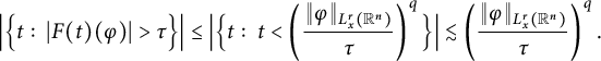 $$ \begin{align*} \Big|\Big\{t:\ |F(t)(\varphi)|>\tau\Big\}\Big| \leq \Big|\Big\{t:\ t<\left(\frac{\|\varphi\|_{L^{r}_{x}(\mathbb R^{n})}}{\tau}\right)^{q}\Big\}\Big| \lesssim\left(\frac{\|\varphi\|_{L^{r}_{x}(\mathbb R^{n})}}{\tau}\right)^{q}. \end{align*} $$
On the other hand, the inequality
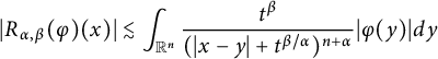 $$ \begin{align*} |R_{\alpha,\beta}(\varphi)(x)|\lesssim\int_{\mathbb R^{n}}\frac{t^{\beta}}{(|x-y|+t^{\beta/\alpha})^{n+\alpha}}|\varphi(y)|dy \end{align*} $$
implies that
 $$ \begin{align*} \|F(t)(\varphi)\|_{L^{\infty}_{t}(I)}=\sup_{t>0}\|R_{\alpha,\beta}(\varphi)\|_{L^{p}_{x}(\mathbb R^{n})}\lesssim t^{-n\beta(1/p-1/p)/\alpha}\|\varphi\|_{L^{p}_{x}(\mathbb R^{n})}, \end{align*} $$
which means that $F(t)$
is a
$F(t)$
is a $(p,\infty )$
-type operator.
$(p,\infty )$
-type operator.
We can find another triplet $(q_{1}, p, r_{1})$
such that
$(q_{1}, p, r_{1})$
such that $q_{1}<q<\infty $
and
$q_{1}<q<\infty $
and $r_{1}<r<p$
satisfying
$r_{1}<r<p$
satisfying
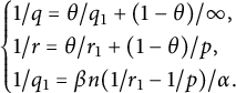 $$ \begin{align*}\begin{cases} 1/q=\theta/q_{1}+(1-\theta)/\infty,\\ 1/r=\theta/r_{1}+(1-\theta)/p,\\ 1/q_{1}=\beta n(1/r_{1}-1/p)/\alpha. \end{cases} \end{align*} $$
The Marcinkiewicz interpolation theorem implies that $F(t)$
is a strong
$F(t)$
is a strong $(r,q)$
-type operator and
$(r,q)$
-type operator and
 $$ \begin{align*} \|R_{\alpha,\beta}(\varphi)\|_{L^{q}_{t}(I; L^{p}_{x}(\mathbb R^{n}))}\lesssim\|\varphi\|_{L^{r}_{x}(\mathbb R^{n})}. \end{align*} $$
(ii) The argument can be also divided into two cases.
Case 3: $p=r$
and
$p=r$
and $q=\infty $
. We have
$q=\infty $
. We have
 $$ \begin{align*} \|R_{\alpha,\beta}(\varphi)\|_{L^{\infty}_{t}(I; L^{p}_{x}(\mathbb R^{n}))}=\sup_{t>0}\|R_{\alpha,\beta}(\varphi)\|_{L^{p}_{x}(\mathbb R^{n})}\lesssim\|\varphi\|_{L^{p}_{x}(\mathbb R^{n})}. \end{align*} $$
Case 4: $p\neq r$
. Because
$p\neq r$
. Because $1/q=\beta n(1/r-1/p)/\alpha $
, upon taking
$1/q=\beta n(1/r-1/p)/\alpha $
, upon taking $q^\ast $
such that
$q^\ast $
such that $1/p+1=1/r+1/q^\ast $
, we obtain
$1/p+1=1/r+1/q^\ast $
, we obtain
 $$ \begin{align*} \|R_{\alpha,\beta}(\varphi)\|_{C_{q}(I; L^{p}_{x}(\mathbb R^{n}))} \lesssim\sup_{t>0}t^{1/q}t^{-\beta n(1/r-1/p)/\alpha}\|\varphi\|_{L^{r}_{x}(\mathbb R^{n})}\lesssim\|\varphi\|_{L^{r}_{x}(\mathbb R^{n})}. \end{align*} $$
On the other hand, for $t\in I$
,
$t\in I$
, $\|R_{\alpha ,\beta }(\varphi )\|_{L^{r}_{x}(\mathbb R^{n})}\lesssim \|\varphi \|_{L^{r}_{x}(\mathbb R^{n})}.$
Consequently,
$\|R_{\alpha ,\beta }(\varphi )\|_{L^{r}_{x}(\mathbb R^{n})}\lesssim \|\varphi \|_{L^{r}_{x}(\mathbb R^{n})}.$
Consequently, $R_{\alpha ,\beta }(\varphi )\in C_{0}(I; L^{r}_{x}(\mathbb R^{n}))$
.
$R_{\alpha ,\beta }(\varphi )\in C_{0}(I; L^{r}_{x}(\mathbb R^{n}))$
.
We then give the following Strichartz-type estimate for $G_{\alpha ,\beta }(g).$
Theorem 2.6 Assume that $\alpha>n$
and
$\alpha>n$
and $0<\beta <1$
. If
$0<\beta <1$
. If $(q,p)$
and
$(q,p)$
and $(\widetilde {q}, \widetilde {p}\kern1pt)$
satisfy
$(\widetilde {q}, \widetilde {p}\kern1pt)$
satisfy
 $$ \begin{align*}\begin{cases} 1\leq \widetilde{p}<p\leq \infty\ \&\ 1<\widetilde{q}<q<\infty,\\ (1/\widetilde{q}-1/q)+ {\beta n}(1/\widetilde{p}-1/p)/{\alpha}=1, \end{cases}\end{align*} $$
then
 $$ \begin{align*}\left\|\int^{t}_{0}\int_{\mathbb R^{n}}G_{t-s}(x-y)g(s,y)dyds\right\|_{L^{q}_{t}(I; L^{p}_{x}(\mathbb R^{n}))}\lesssim \|g\|_{L^{\widetilde{q}}_{t}(I; L^{\widetilde{p}}_{x}(\mathbb R^{n}))}.\end{align*} $$
Proof An application of Lemma 2.3 yields
 $$ \begin{align*} \left\|\int_{\mathbb R^{n}}G_{t-s}(x-y)g(s,y)dy\right\|_{L^{p}_{x}(\mathbb R^{n})}\lesssim |t-s|^{-n\beta(1/\widetilde{p}-1/p)/\alpha}\|g(s,\cdot)\|_{L_{x}^{\widetilde{p}}(\mathbb R^{n})}. \end{align*} $$
It follows from the boundedness of fractional integrals that
 $$ \begin{align*} &\left\|\int^{t}_{0}\int_{\mathbb R^{n}}G_{t-s}(x-y)g(s,y)dyds\right\|_{L^{q}_{t}(I; L^{p}_{x}(\mathbb R^{n}))} \\&\quad\lesssim \left\|\int^{t}_{0}\left\|\int_{\mathbb R^{n}}G_{t-s}(x-y)g(s,y)dy\right\|_{L^{p}_{x}(\mathbb R^{n})}ds\right\|_{L^{q}_{t}(I)}\\ &\quad\lesssim \left\|\int^{t}_{0}|t-s|^{-n\beta(1/\widetilde{p}-1/p)/\alpha}\|g(s,\cdot)\|_{L_{x}^{\widetilde{p}}(\mathbb R^{n})}ds\right\|_{L^{q}_{t}(I)}\\ &\quad\lesssim \|g\|_{L^{\widetilde{q}}_{t}(I; L^{\widetilde{p}}_{x}(\mathbb R^{n}))}, \end{align*} $$
which finishes the proof.
2.3 Other space–time estimates for
$G_{\alpha ,\beta }$

We will establish the following space–time estimate for $G_{\alpha ,\beta }.$
Theorem 2.7 Given $\alpha>n$
and
$\alpha>n$
and $0<\beta <1$
. For
$0<\beta <1$
. For $b>0$
and
$b>0$
and $T>0$
, let
$T>0$
, let $r_{0}=n\beta b/\alpha $
and
$r_{0}=n\beta b/\alpha $
and $I=[0, T)$
. Assume that
$I=[0, T)$
. Assume that $r\geq r_{0}>1$
and that
$r\geq r_{0}>1$
and that $(q,p,r)$
is a triplet satisfying
$(q,p,r)$
is a triplet satisfying $1\leq r\leq p<\infty $
,
$1\leq r\leq p<\infty $
, $1/q=\beta n(1/r-1/p)/\alpha $
, and
$1/q=\beta n(1/r-1/p)/\alpha $
, and $p>b+1$
.
$p>b+1$
.
-
(i) If
$g(\cdot ,\cdot )\in L^{q/(b+1)}_{t}(I; L^{p/(b+1)}_{x}(\mathbb R^{n}))$
, then
$$ \begin{align*} &\|G_{\alpha,\beta}(g)\|_{L^{\infty}_{t}(I; L^{r}_{x}(\mathbb R^{n}))}\\&\quad\lesssim \left\{\begin{aligned} &T^{1-\beta nb/(r\alpha)}\|g\|_{L^{q/(b+1)}_{t}(I; L^{p/(b+1)}_{x}(\mathbb R^{n}))}, &p<r(b+1),\\ &T^{1-n\beta b/(r\alpha)}\Big\||g|^{1/(b+1)}\Big\|^{\theta(b+1)}_{L^{\infty}_{t}(I; L^{r}_{x}(\mathbb R^{n}))}\cdot\Big\||g|^{1/(b+1)}\Big\|^{(1-\theta)(b+1)}_{L^{q}_{t}(I; L^{p}_{x}(\mathbb R^{n}))}, &p\geq r(b+1), \end{aligned}\right. \end{align*} $$
where
$\theta =(p/(b+1)-r)/(p-r)$
. -
(ii) If
$g(\cdot ,\cdot )\in L^{q/(b+1)}_{t}(I; L^{p/(b+1)}_{x}(\mathbb R^{n}))$
, then
$$ \begin{align*}&\|G_{\alpha,\beta}(g)\|_{L^{q}_{t}(I; L^{p}_{x}(\mathbb R^{n}))}\\&\quad\lesssim \left\{\begin{aligned} &T^{1-nb\beta/(r\alpha)}\|g\|_{L^{q/(b+1)}_{t}(I; L^{p/(b+1)}_{x}(\mathbb R^{n}))}, &p<r(b+1),\\ &T^{1-nb\beta/(r\alpha)}\Big\||g|^{1/(b+1)}\Big\|^{\theta(b+1)}_{L^{\infty}_{t}(I; L^{r}_{x}(\mathbb R^{n}))}\cdot\Big\||g|^{1/(b+1)}\Big\|^{(1-\theta)(b+1)}_{L^{q}_{t}(I; L^{p}_{x}(\mathbb R^{n}))}, &p\geq r(b+1), \end{aligned}\right.\end{align*} $$
where
$\theta =(p/(b+1)-r)/(p-r)$
.


Proof (i) For the case $p<r(b+1)$
, we have
$p<r(b+1)$
, we have
 $$ \begin{align*} \|G_{\alpha,\beta}(g)\|_{L^{\infty}_{t}(I; L^{r}_{x}(\mathbb R^{n}))}&= \sup_{t\in I}\left\|\int^{t}_{0}\int_{\mathbb R^{n}}G_{t-s}(x-y)g(s,y)dyds\right\|_{L^{r}_{x}(\mathbb R^{n})}\\ &\lesssim \sup_{t\in I}\int^{t}_{0}\left\|\int_{\mathbb R^{n}}G_{t-s}(x-y)g(s,y)dy\right\|_{L^{r}_{x}(\mathbb R^{n})}ds. \end{align*} $$
Take $q^\ast $
such that
$q^\ast $
such that $(b+1)/p+1/q^{\ast }=1+1/r$
. Then, by Lemma 2.3,
$(b+1)/p+1/q^{\ast }=1+1/r$
. Then, by Lemma 2.3,
 $$ \begin{align*} \left\|\int_{\mathbb R^{n}}G_{t-s}(x-y)g(s,y)dy\right\|_{L^{r}_{x}(\mathbb R^{n})}\lesssim (t-s)^{-n\beta(1-1/q^\ast)/\alpha}\|g(s,\cdot)\|_{L^{p/(b+1)}_{x}(\mathbb R^{n})}, \end{align*} $$
which implies that
 $$ \begin{align*}\|G_{\alpha,\beta}(g)\|_{L^{\infty}_{t}(I; L^{r}(\mathbb R^{n}))}\lesssim\sup_{t\in I}\int^{t}_{0}(t-s)^{-n\beta((b+1)/p-1/r)/\alpha}\|g(s,\cdot)\|_{L^{p/(b+1)}_{x}(\mathbb R^{n})}ds.\end{align*} $$
Let $\widetilde {q}$
be the conjugate of
$\widetilde {q}$
be the conjugate of $q/(b+1)$
, i.e.,
$q/(b+1)$
, i.e., $(b+1)/q+1/\widetilde {q}=1$
. Because
$(b+1)/q+1/\widetilde {q}=1$
. Because $r>r_{0}:=b\beta n/\alpha $
, then
$r>r_{0}:=b\beta n/\alpha $
, then
 $$ \begin{align*} 0<1-n\beta((b+1)/p-1/r)\widetilde{q}/\alpha=\widetilde{q}(1-b\beta n/r\alpha)<1. \end{align*} $$
A direct computation, together with change of variables, gives
 $$ \begin{align*} \Bigg(\int^{t}_{0}(t-s)^{-n\beta((b+1)/p-1/r)\widetilde{q}/\alpha}ds\Bigg)^{1/\widetilde{q}}\lesssim T^{1/\widetilde{q}-n\beta((b+1)/p-1/r)/\alpha}. \end{align*} $$
Then we obtain
 $$ \begin{align*} &\|G_{\alpha,\beta}(g)\|_{L^{\infty}(I; L^{r})}\\&\quad\lesssim \sup_{t\in I}\Bigg(\int^{t}_{0}(t-s)^{-n\beta((b+1)/p-1/r)\widetilde{q}/\alpha}ds\Bigg)^{1/\widetilde{q}} \Bigg(\int^{t}_{0}\|g(s,\cdot)\|^{q/(b+1)}_{L^{p/(b+1)}_{x}(\mathbb R^{n})}ds\Bigg)^{(b+1)/q}\\ &\quad\lesssim T^{1/\widetilde{q}-n\beta((b+1)/p-1/r)/\alpha}\|g\|_{L^{q/(b+1)}_{t}(I; L^{p/(b+1)}_{x}(\mathbb R^{n}))}\\ &\quad\lesssim T^{1-b\beta n/r\alpha}\|g\|_{L^{q/(b+1)}_{t}(I; L^{p/(b+1)}_{x}(\mathbb R^{n}))}, \end{align*} $$
where in the last inequality we have used the fact that
 $$ \begin{align*} 1/\widetilde{q}-n\beta[(b+1)/p-1/r]/\alpha=1-b\beta n/r\alpha. \end{align*} $$
When $p\geq r(b+1)$
, Lemma 2.3 gives
$p\geq r(b+1)$
, Lemma 2.3 gives
 $$ \begin{align*} &\|G_{\alpha,\beta}(g)\|_{L^{\infty}_{t}(I; L^{r}_{x}(\mathbb R^{n}))}\lesssim\sup_{t\in I}\int^{t}_{0}\left\|\int_{\mathbb R^{n}}G_{t-s}(x-y)g(s,y)dy\right\|_{L^{r}_{x}(\mathbb R^{n})}ds\\&\quad\lesssim\sup_{t\in I}\int^{t}_{0}\big\|g(s,\cdot)\big\|_{L^{r}_{x}(\mathbb R^{n})}ds. \end{align*} $$
Notice that $\|g(s,\cdot )\|_{L^{r}_{x}(\mathbb R^{n})}=\||g(s,\cdot )|^{1/(b+1)}\|_{L^{r(b+1)}_{x}(\mathbb R^{n})}^{b+1}.$
Hence,
$\|g(s,\cdot )\|_{L^{r}_{x}(\mathbb R^{n})}=\||g(s,\cdot )|^{1/(b+1)}\|_{L^{r(b+1)}_{x}(\mathbb R^{n})}^{b+1}.$
Hence,
 $$ \begin{align*} \|G_{\alpha,\beta}(g)\|_{L^{\infty}_{t}(I; L^{r}_{x}(\mathbb R^{n}))}\lesssim\sup_{t\in I}\int^{t}_{0}\Big\||g(s,\cdot)|^{1/(b+1)}\Big\|_{L^{r(b+1)}_{x}(\mathbb R^{n})}^{b+1}ds. \end{align*} $$
Take $\theta \in (0,1)$
such that
$\theta \in (0,1)$
such that $1/(rb+r)=\theta /r+(1-\theta )/p$
. Let
$1/(rb+r)=\theta /r+(1-\theta )/p$
. Let $p_{1}=(b(1+\theta ))^{-1}$
and
$p_{1}=(b(1+\theta ))^{-1}$
and $q_{1}=p/(r(b+1)(1-\theta ))$
such that
$q_{1}=p/(r(b+1)(1-\theta ))$
such that $1/p_{1}+1/q_{1}=1$
. Applying Hölder’s inequality on the spatial variable, we obtain
$1/p_{1}+1/q_{1}=1$
. Applying Hölder’s inequality on the spatial variable, we obtain
 $$ \begin{align*} &\||g(s,\cdot)|^{1/(b+1)}\|_{L^{r(b+1)}_{x}(\mathbb R^{n})}^{b+1}\\&\quad\lesssim \left\{\int_{\mathbb R^{n}}|g(s,x)|^{r\theta p_{1}}dx\right\}^{1/(rp_{1})}\left\{\int_{\mathbb R^{n}}|g(s,x)|^{r(1-\theta) q_{1}}dx\right\}^{1/(rq_{1})}\\ &\quad\lesssim \left\{\int_{\mathbb R^{n}}|g(s,x)|^{r/(b+1)}dx\right\}^{\theta(b+1)/r}\left\{\int_{\mathbb R^{n}}|g(s,x)|^{p/(b+1)}dx\right\}^{(b+1)(1-\theta)/p}, \end{align*} $$
which indicates that
 $$ \begin{align*} &\|G_{\alpha,\beta}(g)\|_{L^{\infty}_{t}(I; L^{r}_{x}(\mathbb R^{n}))}\\[4pt]&\quad\lesssim \sup_{t\in I}\int^{t}_{0}\big\||g(s,\cdot)|^{1/(b+1)}\big\|_{L^{r}_{x}(\mathbb R^{n})}^{\theta(b+1)}\cdot \big\||g(s,\cdot)|^{1/(b+1)}\big\|_{L^{p}_{x}(\mathbb R^{n})}^{(1-\theta)(b+1)}ds\\[4pt] &\quad\lesssim \big\||g(\cdot,\cdot)|^{1/(b+1)}\big\|^{(b+1)\theta}_{L^{\infty}_{t}(I; L^{r}_{x}(\mathbb R^{n}))}\sup_{t\in I}\int^{t}_{0}\big\||g(s,\cdot)|^{1/(b+1)}\big\|_{L^{p}_{x}(\mathbb R^{n})}^{(1-\theta)(b+1)}ds\\[4pt] &\quad\lesssim \big\||g(\cdot,\cdot)|^{1/(b+1)}\big\|^{(b+1)\theta}_{L^{\infty}_{t}(I; L^{r}_{x}(\mathbb R^{n}))}\sup_{t\in I}\left\{\left(\int^{t}_{0}1ds\right)^{1-(b+1)(1-\theta)/q}\right.\\[4pt] &\qquad \times\left.\left(\int^{t}_{0}\big\||g(s,\cdot)|^{1/(b+1)}\big\|_{L^{p}_{x}(\mathbb R^{n})}^{(1-\theta)(b+1)q/(1-\theta)(1+b)}ds\right)^{(b+1)(1-\theta)/q}\right\}\\[4pt] &\quad\lesssim T^{1-(b+1)(1-\theta)/q}\big\||g(\cdot,\cdot)|^{1/(b+1)}\big\|^{(b+1)\theta}_{L^{\infty}_{t}(I; L^{r}_{x}(\mathbb R^{n}))}\big\||g|^{1/(b+1)}\big\|^{(b+1)(1-\theta)}_{L^{q}_{t}(I; L^{p}(\mathbb R^{n}))}. \end{align*} $$
Since $1/q=\beta n(1/r-1/p)/\alpha $
and
$1/q=\beta n(1/r-1/p)/\alpha $
and $\theta =(p-rb-r)/((p-r)(b+1))$
, then
$\theta =(p-rb-r)/((p-r)(b+1))$
, then
 $$ \begin{align*} \|G_{\alpha,\beta}(g)\|_{L^{\infty}_{t}(I; L^{r}_{x}(\mathbb R^{n}))}\lesssim T^{1-n\beta b/(r\alpha)}\Big\||g|^{1/(b+1)}\Big\|^{\theta(b+1)}_{L^{\infty}_{t}(I; L^{r}_{x}(\mathbb R^{n}))}\Big\||g|^{1/(b+1)}\Big\|^{(1-\theta)(b+1)}_{L^{q}_{t}(I; L^{p}_{x}(\mathbb R^{n}))}. \end{align*} $$
This completes the proof of (i).
(ii) For the case $p<r(b+1)$
, using Minkowski’s inequality and Lemma 2.3, we obtain
$p<r(b+1)$
, using Minkowski’s inequality and Lemma 2.3, we obtain
 $$ \begin{align*} &\|G_{\alpha,\beta}(g)\|_{L^{q}_{t}(I; L^{p}_{x}(\mathbb R^{n}))} \\[4pt]&\quad\lesssim \left\{\int^{T}_{0}\left(\int^{t}_{0}\Big\|\int_{\mathbb R^{n}}G_{t-s}(x-y)g(s,y)dy\Big\|_{L^{p}_{x}(\mathbb R^{n})}ds\right)^{q}dt\right\}^{1/q}\\[4pt] &\quad\lesssim \left\{\int^{T}_{0} \left(\int^{t}_{0}(t-s)^{-n\beta((b+1)/p-1/p)/\alpha}\|g(s,\cdot)\|_{L^{p/(b+1)}_{x}(\mathbb R^{n})}ds\right)^{q}dt\right\}^{1/q}\\[4pt] &\quad= \left\|\int^{t}_{0}(t-s)^{-n\beta b/p\alpha}\|g(s,\cdot)\|_{L^{p/(b+1)}_{x}(\mathbb R^{n})}ds\right\|_{L^{q}_{t}(I)}. \end{align*} $$
Let $\chi $
be the number such that
$\chi $
be the number such that $1/q+1=(1+b)/q+1/\chi $
. An application of Young’s inequality gives
$1/q+1=(1+b)/q+1/\chi $
. An application of Young’s inequality gives
 $$ \begin{align*} \|G_{\alpha,\beta}(g)\|_{L^{q}_{t}(I; L^{p}_{x}(\mathbb R^{n}))}&\lesssim \|g(\cdot,\cdot)\|_{L^{q/(b+1)}_{t}(I; L^{p/(b+1)}_{x}(\mathbb R^{n}))}\Bigg(\int^{T}_{0}t^{-n\beta b\chi/p\alpha}dt\Bigg)^{1/\chi}\\[4pt] &\lesssim T^{1-n\beta b/r\alpha}\|g(\cdot,\cdot)\|_{L^{q/(b+1)}_{t}(I; L^{p/(b+1)}_{x}(\mathbb R^{n}))}, \end{align*} $$
where in the last inequality we have used the fact that $1/q=n\beta (1/r-1/p)/\alpha $
.
$1/q=n\beta (1/r-1/p)/\alpha $
.
For the case $p\geq r(b+1)$
, we apply Lemma 2.3 again to get
$p\geq r(b+1)$
, we apply Lemma 2.3 again to get
 $$ \begin{align*} \|G_{\alpha,\beta}(g)\|_{L^{q}_{t}(I; L^{p}_{x}(\mathbb R^{n}))}&\lesssim \left\|\int^{t}_{0}\left\|\int_{\mathbb R^{n}}G_{t-s}(x-y)g(s,y)dy\right\|_{L^{p}_{x}(\mathbb R^{n})}ds\right\|_{L^{q}_{t}(I)}\\ &\lesssim \left\|\int^{t}_{0}(t-s)^{-n\beta(1/r-1/p)/\alpha} \left\||g(s,\cdot)|^{1/(b+1)}\right\|_{L^{p}_{x}(\mathbb R^{n})}ds\right\|_{L^{q}_{t}(I)}. \end{align*} $$
Choose $\theta \in (0,1)$
such that
$\theta \in (0,1)$
such that $1/(b+1)=\theta +(1-\theta )r/p$
. Letting
$1/(b+1)=\theta +(1-\theta )r/p$
. Letting $p_{2}=(b+b\theta )^{-1}$
and
$p_{2}=(b+b\theta )^{-1}$
and $q_{2}=p/(r(b+1)(1-\theta ))$
, we use Hölder’s inequality on the spatial variable to deduce
$q_{2}=p/(r(b+1)(1-\theta ))$
, we use Hölder’s inequality on the spatial variable to deduce
 $$ \begin{align*} &\int^{t}_{0}(t-s)^{-\beta(1/r-1/p)/\alpha}\Big\||g(s,\cdot)|^{1/(b+1)}\Big\|_{L^{r(b+1)}_{x}(\mathbb R^{n})}^{b+1}ds\\ &\lesssim\int^{t}_{0}(t-s)^{-n\beta(1/r-1/p)/\alpha}\Bigg(\int_{\mathbb R^{n}}|g(s,x)|^{r\theta p_{2}}dx\Bigg)^{1/(rp_{2})}\Bigg(\int_{\mathbb R^{n}}|g(s,x)|^{r(1-\theta)q_{2}}dx\Bigg)^{1/(rq_{2})}ds\\ &\lesssim\int^{t}_{0}(t-s)^{-n\beta(1/r-1/p)/\alpha}\big\||g(s,\cdot)|^{1/(b+1)}\big\|^{\theta(b+1)}_{L^{r}_{x}(\mathbb R^{n})} \big\||g(s,\cdot)|^{1/(b+1)}\big\|^{(1-\theta)(b+1)}_{L^{p}_{x}(\mathbb R^{n})}ds\\ &\lesssim\big\||g(s,\cdot)|^{1/(b+1)}\big\|^{\theta(b+1)}_{L^{\infty}_{t}(I;L^{r}_{x}(\mathbb R^{n}))}\int^{t}_{0}(t-s)^{-n\beta(1/r-1/p)/\alpha} \big\||g(s,\cdot)|^{1/(b+1)}\big\|^{(1-\theta)(b+1)}_{L^{p}_{x}(\mathbb R^{n})}ds, \end{align*} $$
which gives
 $$ \begin{align*} \|G_{\alpha,\beta}(g)\|_{L^{q}_{t}(I; L^{p}_{x}(\mathbb R^{n}))}&\lesssim \big\||g(\cdot,\cdot)|^{1/(b+1)}\big\|^{\theta(b+1)}_{L^{\infty}_{t}(I;L^{r}_{x}(\mathbb R^{n}))}\\ &\quad\times\left\|\int^{t}_{0}\!(t\kern1.3pt{-}\kern1.3pts)^{-n\beta(1/r-1/p)/\alpha} \big\||g(s,\cdot)|^{1/(b+1)}\big\|^{(1-\theta)(b+1)}_{L^{p}_{x}(\mathbb R^{n})}ds\right\|_{L^{q}_{t}(I)}\!\kern-1pt. \end{align*} $$
Suppose that $\widetilde {\chi }$
obeys
$\widetilde {\chi }$
obeys $1/q+1=(1+b)(1-\theta )/q+1/\widetilde {\chi }$
. Young’s inequality on the time variable gives
$1/q+1=(1+b)(1-\theta )/q+1/\widetilde {\chi }$
. Young’s inequality on the time variable gives
 $$ \begin{align*} &\|G_{\alpha,\beta}(g)\|_{L^{q}_{t}(I; L^{p}_{x}(\mathbb R^{n}))}\\&\quad\lesssim \big\||g(\cdot,\cdot)|^{1/(b+1)}\big\|^{\theta(b+1)}_{L^{\infty}_{t}(I;L^{r}_{x}(\mathbb R^{n}))}\big\||g(\cdot,\cdot)|^{1/(b+1)}\big\|^{(b+1)(1-\theta)}_{L^{q}_{t}(I; L^{p}_{x}(\mathbb R^{n}))}\\ &\qquad\times\Bigg(\int^{T}_{0}t^{-n\beta(1/r-1/p)\widetilde{\chi}/\alpha}dt\Bigg)^{1/\widetilde{\chi}}\\ &\quad\lesssim T^{1-b\beta n/(r\alpha)}\||g(\cdot,\cdot)|^{1/(b+1)}\big\|^{\theta(b+1)}_{L^{\infty}_{t}(I;L^{r}_{x}(\mathbb R^{n}))}\big\||g(\cdot,\cdot)|^{1/(b+1)}\big\|^{(b+1)(1-\theta)}_{L^{q}_{t}(I; L^{p}_{x}(\mathbb R^{n}))}, \end{align*} $$
where in the last inequality we have used the fact that $1/\widetilde {\chi }-n\beta (1/r-1/p)/\alpha =1-b\beta n/(r\alpha )$
. This completes the proof of Theorem 2.7.
$1/\widetilde {\chi }-n\beta (1/r-1/p)/\alpha =1-b\beta n/(r\alpha )$
. This completes the proof of Theorem 2.7.
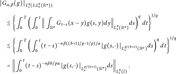
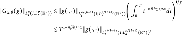
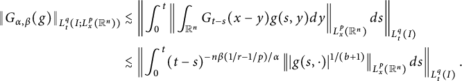
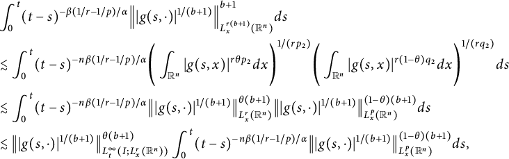
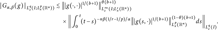
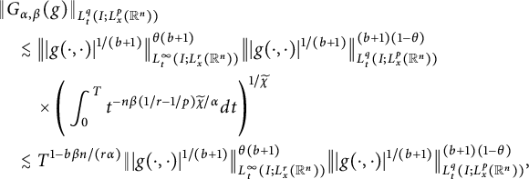
Theorem 2.8 Let $\alpha>n$
and
$\alpha>n$
and $0<\beta <1$
. For
$0<\beta <1$
. For $b>0$
and
$b>0$
and $T>0$
, let
$T>0$
, let $r_{0}=bn\beta /\alpha $
,
$r_{0}=bn\beta /\alpha $
, $I=[0,T)$
. Assume that
$I=[0,T)$
. Assume that $r\geq r_{0}>1$
and
$r\geq r_{0}>1$
and $(q,p,r)$
is a triplet satisfying
$(q,p,r)$
is a triplet satisfying $1\leq r\leq p<\infty $
,
$1\leq r\leq p<\infty $
, $1/q=\beta n(1/r-1/p)/\alpha $
, and
$1/q=\beta n(1/r-1/p)/\alpha $
, and $p>b+1$
.
$p>b+1$
.
-
(i) If
$g\in C_{q/(b+1)}(I; L^{p/(b+1)}_{x}(\mathbb R^{n}))$
, then
$$ \begin{align*} &\|G_{\alpha,\beta}(g)\|_{L^{\infty}_{t}(I; L^{r}_{x}(\mathbb R^{n}))}\\&\quad\lesssim \left\{\begin{aligned} &T^{1-b\beta n/(r\alpha)}\|g\|_{C_{q/(b+1)}(I; L^{p/(b+1)}_{x}(\mathbb R^{n}))},\ &p<r(b+1),\\ &T^{1-bn\beta/(r\alpha)}\big\||g|^{1/(b+1)}\big\|^{\theta(b+1)}_{L^{\infty}_{t}(I; L^{r}_{x}(\mathbb R^{n}))} \big\||g|^{1/(b+1)}\big\|^{(1-\theta)(b+1)}_{C_{q}(I; L^{r}_{x}(\mathbb R^{n}))},\ &p\geq r(b+1), \end{aligned} \right.\end{align*} $$
where
$\theta =(p/(b+1)-r)/(p-r)$
. -
(ii) If
$g\in C_{q/(b+1)}(I; L^{p/(b+1)}_{x}(\mathbb R^{n}))$
, then
$$ \begin{align*}&\|G_{\alpha,\beta}(g)\|_{C_{q}(I; L^{p}_{x}(\mathbb R^{n}))}\\&\quad\lesssim \left\{\begin{aligned} &T^{1-b\beta n/(r\alpha)}\|g\|_{C_{q/(b+1)}(I; L^{p/(b+1)}_{x}(\mathbb R^{n}))},\ &p<r(b+1),\\ &T^{1-bn\beta/(r\alpha)}\big\||g|^{1/(b+1)}\big\|^{\theta(b+1)}_{L^{\infty}_{t}(I; L^{r}_{x}(\mathbb R^{n}))} \big\||g|^{1/(b+1)}\big\|^{(1-\theta)(b+1)}_{C_{q}(I; L^{p}_{x}(\mathbb R^{n}))},\ &p\geq r(b+1), \end{aligned} \right.\end{align*} $$
where
$\theta =(p/(b+1)-r)/(p-r)$
.


Proof (i) We first consider the case $p<r(b+1)$
, and it follows from Lemma 2.3 that
$p<r(b+1)$
, and it follows from Lemma 2.3 that
 $$ \begin{align*}\left\|\int_{\mathbb R^{n}}G_{t-s}(x-y)g(s,y)dy\right\|_{L^{r}_{x}(\mathbb R^{n})}\lesssim (t-s)^{-n\beta[(b+1)/p-1/r]/\alpha}\|g(s,\cdot)\|_{L^{p/(b+1)}_{x}(\mathbb R^{n})},\end{align*} $$
which implies that
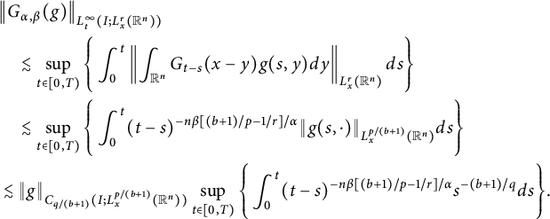 $$ \begin{align*} &\big\|G_{\alpha,\beta}(g)\big\|_{L^{\infty}_{t}(I; L^{r}_{x}(\mathbb R^{n}))}\\&\quad\lesssim \sup_{t\in[0, T)}\Bigg\{\int^{t}_{0}\left\|\int_{\mathbb R^{n}}G_{t-s}(x-y)g(s,y)dy\right\|_{L^{r}_{x}(\mathbb R^{n})}ds\Bigg\}\\ &\quad\lesssim \sup_{t\in[0, T)}\Bigg\{\int^{t}_{0}(t-s)^{-n\beta[(b+1)/p-1/r]/\alpha}\|g(s,\cdot)\|_{L^{p/(b+1)}_{x}(\mathbb R^{n})}ds\Bigg\}\\ &\lesssim \|g\|_{C_{q/(b+1)}(I; L^{p/(b+1)}_{x}(\mathbb R^{n}))}\sup_{t\in[0, T)}\Bigg\{\int^{t}_{0}(t-s)^{-n\beta[(b+1)/p-1/r]/\alpha}s^{-(b+1)/q}ds\Bigg\}. \end{align*} $$
A direct computation, together with the change of variables: $u=s/t$
, gives
$u=s/t$
, gives
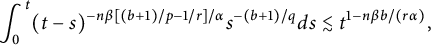 $$ \begin{align*} \int^{t}_{0}(t-s)^{-n\beta[(b+1)/p-1/r]/\alpha}s^{-(b+1)/q}ds\lesssim t^{1-n\beta b/(r\alpha)}, \end{align*} $$
which indicates that
 $$ \begin{align*} \|G_{\alpha,\beta}(g)\|_{L^{\infty}_{t}(I; L^{r}_{x}(\mathbb R^{n}))}\lesssim T^{1-n\beta b/r\alpha}\|g\|_{C_{q/(b+1)}(I; L^{p/(b+1)}_{x}(\mathbb R^{n}))}. \end{align*} $$
Now, we consider the case $p\geq (b+1)r$
. By Lemma 2.3, we have
$p\geq (b+1)r$
. By Lemma 2.3, we have
 $$ \begin{align*} \left\|\int_{\mathbb R^{n}}G_{t-s}(x-y)g(s,y)dy\right\|_{L^{r}_{x}(\mathbb R^{n})}\lesssim \|g(s,\cdot)\|_{L^{r}_{x}(\mathbb R^{n})}. \end{align*} $$
If $\theta \in (0,1)$
,
$\theta \in (0,1)$
, $p_{3}=\frac {1}{(b+1)\theta }$
, and
$p_{3}=\frac {1}{(b+1)\theta }$
, and $ q_{3}=\frac {p}{r(b+1)(1-\theta )}$
, then we obtain
$ q_{3}=\frac {p}{r(b+1)(1-\theta )}$
, then we obtain
 $$ \begin{align*} \|G_{\alpha,\beta}(g)\|_{L^{\infty}_{t}(I; L^{r}_{x}(\mathbb R^{n}))}&= \sup_{t\in I}\Bigg\|\int^{t}_{0}\int_{\mathbb R^{n}}G_{t-s}(x-y)g(s,y)dyds\Bigg\|_{L^{r}_{x}(\mathbb R^{n})}\\ &\lesssim \sup_{t\in I}\int^{t}_{0}\|g(s,\cdot)\|_{L^{r}_{x}(\mathbb R^{n})}ds. \end{align*} $$
Notice that $1-(b+1)(1-\theta )/q=1-b\beta n/(r\alpha )$
. An application of Hölder’s inequality gives
$1-(b+1)(1-\theta )/q=1-b\beta n/(r\alpha )$
. An application of Hölder’s inequality gives
 $$ \begin{align*} &\|G_{\alpha,\beta}(g)\|_{L^{\infty}_{t}(I; L^{r}_{x}(\mathbb R^{n}))}\\&\lesssim \sup_{t\in I}\int^{t}_{0}\big\||g(s,\cdot)|^{1/(b+1)}\big\|^{b+1}_{L^{r(b+1)}_{x}(\mathbb R^{n})}ds\\ &\lesssim \sup_{t\in [0,T)}\left\{\int^{t}_{0}\big\||g(s,\cdot)|^{1/(b+1)}\big\|^{\theta(b+1)}_{L^{r}_{x}(\mathbb R^{n})}\big\||g(s,\cdot)|^{1/(b+1)}\big\|^{(1-\theta)(b+1)}_{L^{p}_{x}(\mathbb R^{n})}ds\right\}\\ &\lesssim \big\||g|^{1/(b+1)}\big\|^{\theta(b+1)}_{L^{\infty}_{t}(I;L^{r}_{x}(\mathbb R^{n}))}\big\||g|^{1/(b+1)}\big\|^{(1-\theta)(b+1)}_{C_{q}(I;L^{p}_{x}(\mathbb R^{n}))}\sup_{t\in [0,T)}\left\{\int^{t}_{0}s^{-(b+1)(1-\theta)/q}ds\right\}\\ &\lesssim T^{1-(b+1)(1-\theta)/q}\big\||g|^{1/(b+1)}\big\|^{\theta(b+1)}_{L^{\infty}_{t}(I;L^{r}_{x}(\mathbb R^{n}))}\big\||g|^{1/(b+1)}\big\|^{(1-\theta)(b+1)}_{C_{q}(I;L^{p}_{x}(\mathbb R^{n}))}. \end{align*} $$
We begin to prove (ii). Let $g\in C_{q/(b+1)}(I; L^{p/(b+1)}_{x}(\mathbb R^{n}))$
. For the case
$g\in C_{q/(b+1)}(I; L^{p/(b+1)}_{x}(\mathbb R^{n}))$
. For the case $p<r(b+1)$
, we have
$p<r(b+1)$
, we have
 $$ \begin{align*} \Bigg\|\int_{\mathbb R^{n}}G_{t-s}(x-y)g(s,y)dy\Bigg\|_{L^{p}_{x}(\mathbb R^{n})}\lesssim (t-s)^{-n\beta b/p\alpha}\|g(s,\cdot)\|_{L^{p/(b+1)}_{x}(\mathbb R^{n})}, \end{align*} $$
and hence
 $$ \begin{align*} \Big\|G_{\alpha,\beta}(g)\Big\|_{C_{q}(I; L^{p}_{x}(\mathbb R^{n}))} &\lesssim \sup_{t\in [0,T)}t^{1/q}\int^{t}_{0}\left\|\int_{\mathbb R^{n}}G_{t-s}(x-y)g(s,y)dy\right\|_{L^{p}_{x}(\mathbb R^{n})}ds\\ &\lesssim \sup_{t\in [0,T)}t^{1/q}\int^{t}_{0}(t-s)^{-n\beta b/p\alpha}\|g(s,\cdot)\|_{L^{p/(b+1)}_{x}(\mathbb R^{n})} ds\\ &\lesssim \|g\|_{C_{q/(b+1)}(I; L^{p/(b+1)}_{x}(\mathbb R^{n}))}\sup_{t\in [0,T)}t^{1/q}\int^{t}_{0}(t-s)^{-n\beta b/p\alpha}s^{-(b+1)/q} ds\\ &\lesssim \|g\|_{C_{q/(b+1)}(I; L^{p/(b+1)}_{x}(\mathbb R^{n}))}T^{1-\beta bn/p\alpha}. \end{align*} $$
For the case $p\geq r(b+1)$
, it holds
$p\geq r(b+1)$
, it holds
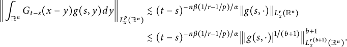 $$ \begin{align*} \left\|\int_{\mathbb R^{n}}G_{t-s}(x-y)g(s,y)dy\right\|_{L^{p}_{x}(\mathbb R^{n})}&\lesssim (t-s)^{-n\beta(1/r-1/p)/\alpha}\|g(s,\cdot)\|_{L^{r}_{x}(\mathbb R^{n})}\\ &\lesssim (t-s)^{-n\beta(1/r-1/p)/\alpha}\big\||g(s,\cdot)|^{1/(b+1)}\big\|^{b+1}_{L^{r(b+1)}_{x}(\mathbb R^{n})}. \end{align*} $$
Taking $\theta =(p-r(b+1))/(p-r)$
, we use the Hölder inequality to deduce
$\theta =(p-r(b+1))/(p-r)$
, we use the Hölder inequality to deduce
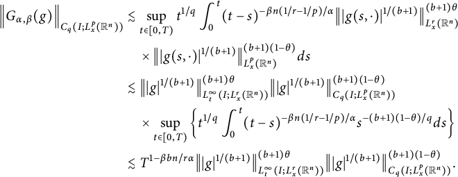 $$ \begin{align*} \Big\|G_{\alpha,\beta}(g)\Big\|_{C_{q}(I; L^{p}_{x}(\mathbb R^{n}))}&\lesssim \sup_{t\in [0,T)}t^{1/q}\int^{t}_{0}(t-s)^{-\beta n(1/r-1/p)/\alpha}\big\||g(s,\cdot)|^{1/(b+1)}\big\|^{(b+1)\theta}_{L^{r}_{x}(\mathbb R^{n})}\\ &\quad\times \big\||g(s,\cdot)|^{1/(b+1)}\big\|^{(b+1)(1-\theta)}_{L^{p}_{x}(\mathbb R^{n})}ds\\ &\lesssim \big\||g|^{1/(b+1)}\big\|^{(b+1)\theta}_{L^{\infty}_{t}(I; L^{r}_{x}(\mathbb R^{n}))} \big\||g|^{1/(b+1)}\big\|^{(b+1)(1-\theta)}_{C_{q}(I;L^{p}_{x}(\mathbb R^{n}))}\\ &\quad\times\sup_{t\in [0, T)}\left\{t^{1/q}\int^{t}_{0}(t-s)^{-\beta n(1/r-1/p)/\alpha}s^{-(b+1)(1-\theta)/q}ds\right\}\\ &\lesssim T^{1-\beta bn/r\alpha}\big\||g|^{1/(b+1)}\big\|^{(b+1)\theta}_{L^{\infty}_{t}(I; L^{r}_{x}(\mathbb R^{n}))} \big\||g|^{1/(b+1)}\big\|^{(b+1)(1-\theta)}_{C_{q}(I;L^{p}_{x}(\mathbb R^{n}))}. \end{align*} $$
This completes the proof of Theorem 2.8.
2.4 Regularities of
$R_{\alpha ,\beta }$
and
$G_{\alpha ,\beta }$


At first, let us recall the following well-known estimates for the fractional heat kernel $K_{\alpha ,t}(\cdot )$
.
$K_{\alpha ,t}(\cdot )$
.
Proposition 2.9 [Reference Miao, Yuan and Zhang52, Lemmas 2.1 and 2.2]
Let $\alpha>0$
.
$\alpha>0$
.
-
(i) There exists a constant C such that
$$ \begin{align*} \Big|K_{\alpha,t}(x)\Big|\simeq C\min\Bigg\{t^{-n/2\alpha},\ \frac{t}{|x|^{n+2\alpha}}\Bigg\}\simeq \frac{Ct}{(t^{1/2\alpha}+|x|)^{n+2\alpha}}. \end{align*} $$
-
(ii) For
$\epsilon>0$
, there exists a constant
$C>0$
such that for
$|h|<t^{1/2\alpha }$
,
$$ \begin{align*} \Big|K_{\alpha,t}(x+h)-K_{\alpha,t}(x)\Big|\leq \frac{Ct}{(t^{1/2\alpha}+|x|)^{n+2\alpha}}\left(\frac{|h|}{t^{1/2\alpha}}\right)^{\epsilon}. \end{align*} $$


Remark 2.10 It is easy to see that in (ii) of Proposition 2.9, the condition $|h|<t^{1/2\alpha }$
can be replaced by
$|h|<t^{1/2\alpha }$
can be replaced by $|h|<|x|/2$
.
$|h|<|x|/2$
.
Below, we investigate the Hölder continuity of the kernel $G_{t}(\cdot )$
.
$G_{t}(\cdot )$
.
Proposition 2.11 Assume that $\alpha>n$
and
$\alpha>n$
and $0<\beta <1$
. For
$0<\beta <1$
. For $\epsilon \in (0, \alpha -n)$
, there exists a positive constant C such that for all
$\epsilon \in (0, \alpha -n)$
, there exists a positive constant C such that for all $x\in \mathbb R^{n}$
and
$x\in \mathbb R^{n}$
and $|h|<t^{\beta /\alpha }$
,
$|h|<t^{\beta /\alpha }$
,
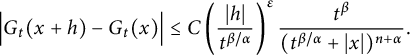 $$ \begin{align} \Big|G_{t}(x+h)-G_{t}(x)\Big|\leq C\left(\frac{|h|}{t^{\beta/\alpha}}\right)^{\epsilon}\frac{t^{\beta}}{(t^{\beta/\alpha}+|x|)^{n+\alpha}}. \end{align} $$
Proof We first verify (2.7) for $|h|<|x|/2$
. Recall that
$|h|<|x|/2$
. Recall that
 $$ \begin{align*} G_{t}(x)=\int^{\infty}_{0}K_{\alpha/2,s}(x)f_{E_{t}}(s)ds, \end{align*} $$
where $f_{E_{t}}(x)=t\beta ^{-1}x^{-1-1/\beta }g_{\beta }(tx^{-1/\beta })$
. An application of change of variables gives
$f_{E_{t}}(x)=t\beta ^{-1}x^{-1-1/\beta }g_{\beta }(tx^{-1/\beta })$
. An application of change of variables gives
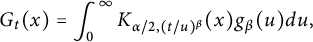 $$ \begin{align*} G_{t}(x)=\int^{\infty}_{0}K_{\alpha/2, (t/u)^{\beta}}(x)g_{\beta}(u)du, \end{align*} $$
which, together with Proposition 2.9(i) with $\epsilon \in (0,\alpha -n)$
, implies that
$\epsilon \in (0,\alpha -n)$
, implies that
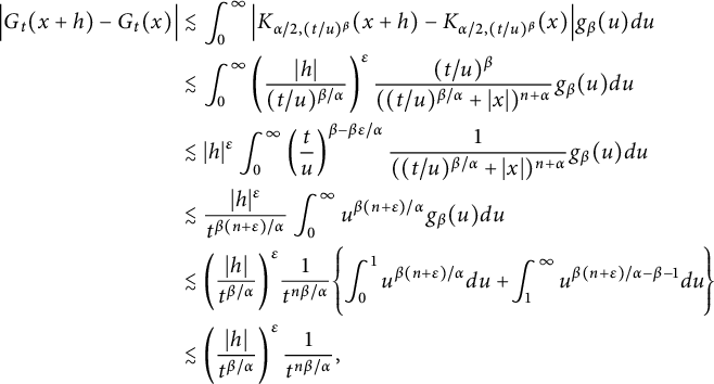 $$ \begin{align} \qquad\!\Big|G_{t}(x+h)-G_{t}(x)\Big|&\lesssim \int^{\infty}_{0}\Big|K_{\alpha/2, (t/u)^{\beta}}(x+h)-K_{\alpha/2, (t/u)^{\beta}}(x)\Big|g_{\beta}(u)du\\ &\lesssim \int^{\infty}_{0}\left(\frac{|h|}{({t}/{u})^{\beta/\alpha}}\right)^{\epsilon} \frac{(t/u)^{\beta}}{((t/u)^{\beta/\alpha}+|x|)^{n+\alpha}}g_{\beta}(u)du\nonumber\\ &\lesssim |h|^{\epsilon}\int^{\infty}_{0}\left(\frac{t}{u}\right)^{\beta-\beta\epsilon/\alpha}\frac{1}{((t/u)^{\beta/\alpha}+|x|)^{n+\alpha}}g_{\beta}(u)du\nonumber\\ &\lesssim \frac{|h|^{\epsilon}}{t^{\beta(n+\epsilon)/\alpha}}\int^{\infty}_{0}u^{\beta(n+\epsilon)/\alpha}g_{\beta}(u)du\nonumber\\ &\lesssim \left(\frac{|h|}{t^{\beta/\alpha}}\right)^{\epsilon}\!\frac{1}{t^{n\beta/\alpha}}\Bigg\{\!\kern-1pt\int^{1}_{0}u^{\beta(n+\epsilon)/\alpha}du+ \!\int^{\infty}_{1}u^{\beta(n+\epsilon)/\alpha-\beta-1}du\kern-1.5pt\Bigg\}\nonumber\\ &\lesssim \left(\frac{|h|}{t^{\beta/\alpha}}\right)^{\epsilon}\frac{1}{t^{n\beta/\alpha}},\nonumber \end{align} $$
where in the last inequality we have used the facts that $\alpha>n$
and
$\alpha>n$
and $0<\epsilon <\alpha -n$
.
$0<\epsilon <\alpha -n$
.
On the other hand, by Proposition 2.9,
 $$ \begin{align*} \Big|K_{\alpha/2,s}(x+h)-K_{\alpha/2,s}(x) \Big|\lesssim\frac{s}{(s^{1/\alpha}+|x|)^{n+\alpha}}\left(\frac{|h|}{s^{1/\alpha}}\right)^{\epsilon} \lesssim\left(\frac{|h|}{s^{1/\alpha}}\right)^{\epsilon}\frac{s}{|x|^{n+\alpha}}, \end{align*} $$
and we have
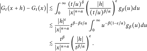 $$ \begin{align} \Big|G_{t}(x+h)-G_{t}(x)\Big|&\lesssim \int^{\infty}_{0}\frac{(t/u)^{\delta}}{|x|^{n+\alpha}}\left(\frac{|h|}{(t/u)^{\beta/\alpha}}\right)^{\epsilon}g_{\beta}(u)du\\ &\lesssim \frac{|h|^{\epsilon}}{|x|^{n+\alpha}}t^{\beta-\beta\epsilon/\alpha}\int^{\infty}_{0}u^{-\beta(1-\epsilon/\alpha)}g_{\beta}(u)du\nonumber\\ &\lesssim \frac{t^{\beta}}{|x|^{n+\alpha}}\left(\frac{|h|}{t^{\beta/\alpha}}\right)^{\epsilon}.\nonumber \end{align} $$
Finally, it can be deuced from (2.8) and (2.9) that
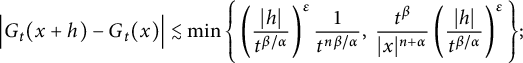 $$ \begin{align*} \Big|G_{t}(x+h)-G_{t}(x)\Big|\lesssim\min\Bigg\{\left(\frac{|h|}{t^{\beta/\alpha}}\right)^{\epsilon}\frac{1}{t^{n\beta/\alpha}},\ \frac{t^{\beta}}{|x|^{n+\alpha}}\left(\frac{|h|}{t^{\beta/\alpha}}\right)^{\epsilon}\Bigg\}; \end{align*} $$
equivalently,
 $$ \begin{align*} \Big|G_{t}(x+h)-G_{t}(x)\Big|\leq C\left(\frac{|h|}{t^{\beta/\alpha}}\right)^{\epsilon}\frac{t^{\beta}}{(t^{\beta/\alpha}+|x|)^{n+\alpha}}. \end{align*} $$
Now, we assume that $|h|<t^{\beta /\alpha }$
. If
$|h|<t^{\beta /\alpha }$
. If $|h|<|x|/2<t^{\beta /\alpha }$
or
$|h|<|x|/2<t^{\beta /\alpha }$
or $|h|<t^{\beta /\alpha }<|x|/2$
, it is obvious that (2.7) holds. Now, we consider the case
$|h|<t^{\beta /\alpha }<|x|/2$
, it is obvious that (2.7) holds. Now, we consider the case $|x|/2<|h|<t^{\beta /\alpha }$
. We split
$|x|/2<|h|<t^{\beta /\alpha }$
. We split $|G_{t}(x+h)-G_{t}(x)|\leq S_{1}+S_{2},$
where
$|G_{t}(x+h)-G_{t}(x)|\leq S_{1}+S_{2},$
where
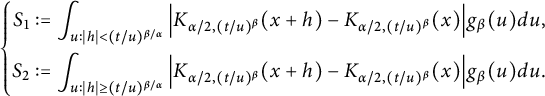 $$ \begin{align*}\left\{\begin{aligned} S_{1}&:=\int_{u: |h|<(t/u)^{\beta/\alpha}}\Big|K_{\alpha/2, (t/u)^{\beta}}(x+h)-K_{\alpha/2, (t/u)^{\beta}}(x)\Big|g_{\beta}(u)du,\\ S_{2}&:=\int_{u: |h|\geq(t/u)^{\beta/\alpha}}\Big|K_{\alpha/2, (t/u)^{\beta}}(x+h)-K_{\alpha/2, (t/u)^{\beta}}(x)\Big|g_{\beta}(u)du. \end{aligned}\right.\end{align*} $$
For $S_{1}$
, since
$S_{1}$
, since $|h|<(t/u)^{\beta /\alpha }$
, it follows from (ii) of Proposition 2.9 that
$|h|<(t/u)^{\beta /\alpha }$
, it follows from (ii) of Proposition 2.9 that
 $$ \begin{align*} S_{1}&\lesssim \int_{u: |h|<(t/u)^{\beta/\alpha}}\left(\frac{|h|}{({t}/{u})^{\beta/\alpha}}\right)^{\epsilon} \frac{(t/u)^{\beta}}{((t/u)^{\beta/\alpha}+|x|)^{n+\alpha}}g_{\beta}(u)du\nonumber\\ &\lesssim \left(\frac{|h|}{t^{\beta/\alpha}}\right)^{\epsilon}\frac{1}{t^{n\beta/\alpha}}\Bigg\{\int^{1}_{0}u^{\beta(n+\epsilon)/\alpha}du+ \int^{\infty}_{1}u^{\beta(n+\epsilon)/\alpha-\beta-1}du\Bigg\}\nonumber\\ &\lesssim \left(\frac{|h|}{t^{\beta/\alpha}}\right)^{\epsilon}\frac{1}{t^{n\beta/\alpha}}. \end{align*} $$
We further divide $S_{2}$
as
$S_{2}$
as $S_{2}\leq S_{2,1}+S_{2,2}$
, where
$S_{2}\leq S_{2,1}+S_{2,2}$
, where
 $$ \begin{align*}\left\{\begin{aligned} S_{2,1}&:=\int_{u: |h|\geq(t/u)^{\beta/\alpha}}\Big|K_{\alpha/2, (t/u)^{\beta}}(x)\Big|g_{\beta}(u)du,\\ S_{2,2}&:=\int_{u: |h|\geq(t/u)^{\beta/\alpha}}\Big|K_{\alpha/2, (t/u)^{\beta}}(x+h)\Big|g_{\beta}(u)du. \end{aligned}\right.\end{align*} $$
Noticing that $|h|\geq (t/u)^{\beta /\alpha }$
, we deduce from (2.5) that
$|h|\geq (t/u)^{\beta /\alpha }$
, we deduce from (2.5) that
 $$ \begin{align*} S_{2,1}&\lesssim \int_{u: |h|\geq(t/u)^{\beta/\alpha}}\left(\frac{|h|}{(t/u)^{\beta/\alpha}}\right)^{\epsilon}\frac{(t/u)^{\beta}}{(|x|+(t/u)^{\beta/\alpha})^{n+\alpha}}g_{\beta}(u)du\\ &\lesssim \left(\frac{|h|}{t^{\beta/\alpha}}\right)^{\epsilon}\frac{1}{t^{n\beta/\alpha}}\int^{\infty}_{0}u^{\beta(n+\epsilon)/\alpha}g_{\beta}(u)du\\ &\lesssim \left(\frac{|h|}{t^{\beta/\alpha}}\right)^{\epsilon}\frac{1}{t^{n\beta/\alpha}}. \end{align*} $$
The term $S_{2,2}$
can be dealt with similar to
$S_{2,2}$
can be dealt with similar to $S_{2,1}$
. Finally, due to
$S_{2,1}$
. Finally, due to $|x|/2<t^{\beta /\alpha }$
, it holds
$|x|/2<t^{\beta /\alpha }$
, it holds
 $$ \begin{align*} \Big|G_{t}(x+h)-G_{t}(x)\Big| \lesssim \left(\frac{|h|}{t^{\beta/\alpha}}\right)^{\epsilon}\frac{1}{t^{n\beta/\alpha}}\lesssim \left(\frac{|h|}{t^{\beta/\alpha}}\right)^{\epsilon}\frac{t^{\beta}}{(t^{\beta/\alpha}+|x|)^{n+\alpha}}, \end{align*} $$
which completes the proof of Proposition 2.11.
Theorem 2.12 Assume that $\alpha>n$
and
$\alpha>n$
and $0<\beta <1$
. If
$0<\beta <1$
. If $p\in [1,\infty ]$
and
$p\in [1,\infty ]$
and $\varphi \in L^{p}(\mathbb R^{n})$
, then
$\varphi \in L^{p}(\mathbb R^{n})$
, then $R_{\alpha ,\beta }(\varphi )(\cdot ,\cdot )$
is continuous on
$R_{\alpha ,\beta }(\varphi )(\cdot ,\cdot )$
is continuous on $\mathbb R^{1+n}_{+}$
.
$\mathbb R^{1+n}_{+}$
.
Proof At first, for fixed $t_{0}>0$
, choose
$t_{0}>0$
, choose $(t_{0},x), ( t_{0},x_{0})\in \mathbb R^{1+n}_{+}$
. By Proposition 2.9 and Hölder’s inequality, we can get
$(t_{0},x), ( t_{0},x_{0})\in \mathbb R^{1+n}_{+}$
. By Proposition 2.9 and Hölder’s inequality, we can get
 $$ \begin{align*} &\left|R_{\alpha,\beta}(\varphi)(t_{0},x)-R_{\alpha,\beta}(\varphi)(t_{0},x_{0})\right| \\&\quad\lesssim \int_{\mathbb R^{n}}\left\{\int^{\infty}_{0}\Big|K_{\alpha/2, (t_{0}/u)^{\beta}}(x-y)-K_{\alpha/2,(t_{0}/u)^{\beta}}(x_{0}-y)\Big|g_{\beta}(u)du\right\}|\varphi(y)|dy\\ &\quad\lesssim \int^{\infty}_{0}\left\{\int_{\mathbb R^{n}}\Big|K_{\alpha/2, (t_{0}/u)^{\beta}}(x-y)-K_{\alpha/2,(t_{0}/u)^{\beta}}(x_{0}-y)\Big|\cdot|\varphi(y)|dy\right\}g_{\beta}(u)du\\ &\quad\lesssim M_{1}+M_{2}, \end{align*} $$
where
 $$ \begin{align*}\left\{\begin{aligned}\! M_{1}&:=\!\int_{u: (t_{0}/u)^{\beta/\alpha}>|x-x_{0}|}\!\left\{\!\int_{\mathbb R^{n}}\Big|K_{\alpha/2, (t_{0}/u)^{\beta}}(x\kern1.3pt{-}\kern1.3pt y)\kern1.3pt{-}\kern1.3pt K_{\alpha/2,(t_{0}/u)^{\beta}}(x_{0}\kern1.3pt{-}\kern1.3pt y)\Big|\cdot |\varphi(y)|dy\!\right\}g_{\beta}(u)du,\\ \!M_{2}&:=\!\int_{u: (t_{0}/u)^{\beta/\alpha}\leq|x-x_{0}|}\!\left\{\!\int_{\mathbb R^{n}}\Big|K_{\alpha/2, (t_{0}/u)^{\beta}}(x\kern1.3pt{-}\kern1.3pt y)\kern1.3pt{-}\kern1.3pt K_{\alpha/2,(t_{0}/u)^{\beta}}(x_{0}\kern1.3pt{-}\kern1.3pt y)\Big| \cdot |\varphi(y)|dy\!\right\}g_{\beta}(u)du.\\ \end{aligned}\right.\end{align*} $$
For $M_{1}$
, since
$M_{1}$
, since $|x-x_{0}|<(t_{0}/u)^{\beta /\alpha }$
, it follows from (ii) of Proposition 2.9 that for
$|x-x_{0}|<(t_{0}/u)^{\beta /\alpha }$
, it follows from (ii) of Proposition 2.9 that for $\epsilon \in (0, \alpha -n/p)$
,
$\epsilon \in (0, \alpha -n/p)$
,
 $$ \begin{align*}\Big|K_{\alpha/2, (t_{0}/u)^{\beta}}(x\kern1.2pt{-}\kern1.2pt y)\kern1.2pt{-}\kern1.2pt K_{\alpha/2,(t_{0}/u)^{\beta}}(x_{0}\kern1.2pt{-}\kern1.2pt y)\Big|\lesssim \left(\frac{|x-x_{0}|}{(t_{0}/u)^{\beta/\alpha}}\right)^{\epsilon} \kern-1pt\!\frac{(t_{0}/u)^{\beta}}{((t_{0}/u)^{\beta/\alpha}+|x\kern1.2pt{-}\kern1.2pt y|)^{n+\alpha}}, \end{align*} $$
and hence
 $$ \begin{align} M_{1}&\lesssim \!\int_{u: (t_{0}/u)^{\beta/\alpha}>|x-x_{0}|}\!\left\{\kern-2pt\int_{\mathbb R^{n}}\!\left(\kern-1.2pt\frac{|x\kern1.2pt{-}\kern1.2pt x_{0}|}{(t_{0}/u)^{\beta/\alpha}}\kern-1.2pt\right)^{\epsilon} \kern-1pt\!\frac{(t_{0}/u)^{\beta}}{((t_{0}/u)^{\beta/\alpha}+|x\kern1.2pt{-}\kern1.2pt y|)^{n+\alpha}}|\varphi(y)|dy\!\right\}g_{\beta}(u)du\\ &\lesssim \int_{u: (t_{0}/u)^{\beta/\alpha}>|x-x_{0}|}\left(\frac{|x-x_{0}|}{(t_{0}/u)^{\beta/\alpha}}\right)^{\epsilon}\frac{(t_{0}/u)^{\beta}}{(t_{0}/u)^{\beta(1+n/\alpha)}} \|\varphi\|_{L_{x}^{p}}(t_{0}/u)^{\beta n/(\alpha p')}g_{\beta}(u)du\nonumber\\ &\lesssim \|\varphi\|_{L_{x}^{p}}\frac{|x-x_{0}|^{\epsilon}}{t_{0}^{\beta(\epsilon+n/p)/\alpha}}\int_{0}^{\infty}u^{\beta(\epsilon+n/p)/\alpha}g_{\beta}(u)du\nonumber\\ &\lesssim \|\varphi\|_{L_{x}^{p}}{t_{0}^{-\beta(\epsilon+n/p)/\alpha}}{|x-x_{0}|^{\epsilon}},\nonumber \end{align} $$
where in the last inequality we have applied (2.2) to estimate the integral as
 $$ \begin{align*} \int_{0}^{\infty}u^{\beta(\epsilon+n/p)/\alpha}g_{\beta}(u)du\lesssim\int_{0}^{1}u^{\beta(\epsilon+n/p)/\alpha} du+\int^{\infty}_{1}u^{\beta(\epsilon+n/ p)/\alpha-\beta-1}du<\infty. \end{align*} $$
For $M_{2}$
, noticing that
$M_{2}$
, noticing that $|x-x_{0}|\geq (t/u)^{\beta /\alpha }$
, we can use (i) of Proposition 2.9 to get
$|x-x_{0}|\geq (t/u)^{\beta /\alpha }$
, we can use (i) of Proposition 2.9 to get
 $$ \begin{align*} &\Big|K_{\alpha/2, (t_{0}/u)^{\beta}}(x-y)-K_{\alpha/2,(t_{0}/u)^{\beta}}(x_{0}-y)\Big|\\ &\lesssim \left(\frac{|x-x_{0}|}{(t_{0}/u)^{\beta/\alpha}}\right)^{\epsilon} \left\{\frac{(t_{0}/u)^{\beta}}{((t_{0}/u)^{\beta/\alpha}+|x-y|)^{n+\alpha}}+\frac{(t_{0}/u)^{\beta}}{((t_{0}/u)^{\beta/\alpha}+|x_{0}-y|)^{n+\alpha}}\right\}. \end{align*} $$
We split $M_{2}\leq M_{2,1}+M_{2,2}$
, where
$M_{2}\leq M_{2,1}+M_{2,2}$
, where
 $$ \begin{align*}\left\{\begin{aligned}\! M_{2,1}&:=\!\int_{u: (t_{0}/u)^{\beta/\alpha}>|x-x_{0}|}\!\left\{\kern-1.2pt\int_{\mathbb R^{n}}\kern-2pt\left(\frac{|x\kern-1.3pt{-}\kern-1.3pt x_{0}|}{(t_{0}/u)^{\beta/\alpha}}\right)^{\epsilon} \!\frac{(t_{0}/u)^{\beta}}{((t_{0}/u)^{\beta/\alpha}+|x-y|)^{n+\alpha}}|\varphi(y)|dy\kern-1.2pt\right\}g_{\beta}(u)du,\\ \!M_{2,2}&:=\!\int_{u: (t_{0}/u)^{\beta/\alpha}>|x-x_{0}|}\!\left\{\kern-1.2pt\int_{\mathbb R^{n}}\kern-2pt\left(\frac{|x\kern-1.3pt{-}\kern-1.3pt x_{0}|}{(t_{0}/u)^{\beta/\alpha}}\right)^{\epsilon} \!\frac{(t_{0}/u)^{\beta}}{((t_{0}/u)^{\beta/\alpha}+|x-y|)^{n+\alpha}}|\varphi(y)|dy\kern-1.2pt\right\}g_{\beta}(u)du. \end{aligned}\right.\end{align*} $$
We can follow the procedure of (2.10) to deduce that
 $$ \begin{align*}M_{2,1}+M_{2,2}\lesssim \|g\|_{L_{x}^{p}}{t_{0}^{-\beta(\epsilon+n/p)/\alpha}}{|x-x_{0}|^{\epsilon}}.\end{align*} $$
This means
 $$ \begin{align} \left|R_{\alpha,\beta}(\varphi)(t_{0},x)-R_{\alpha,\beta}(\varphi)(t_{0},x_{0})\right|\lesssim \|g\|_{L_{x}^{p}}{t_{0}^{-\beta(\epsilon+n/p)/\alpha}}{|x-x_{0}|^{\epsilon}}, \end{align} $$
which indicates that $R_{\alpha ,\beta }(\varphi )(t_{0}, x)$
is continuous with respect to the spatial variable x. Now, we investigate the continuity respect to the time variable t. For fixed
$R_{\alpha ,\beta }(\varphi )(t_{0}, x)$
is continuous with respect to the spatial variable x. Now, we investigate the continuity respect to the time variable t. For fixed $x\in \mathbb R^{n}$
,
$x\in \mathbb R^{n}$
,
 $$ \begin{align*} &R_{\alpha,\beta}(\varphi)(t,x)-R_{\alpha,\beta}(\varphi)(t_{0},x) \\&\quad= \int_{\mathbb R^{n}}\left(G_{t}(x-y)-G_{t_{0}}(x-y)\right)\varphi(y)dy\\ &\quad= \int_{\mathbb R^{n}}\left\{\int^{\infty}_{0}\left(K_{\alpha/2, (t/u)^{\beta}}(x-y)-K_{\alpha/2,(t_{0}/u)^{\beta}}(x-y)\right)g_{\beta}(u)du\right\}\varphi(y)dy\\ &\quad= \int^{\infty}_{0}\left\{\int_{\mathbb R^{n}}\left(K_{\alpha/2,(t/u)^{\beta}}(x-y)-K_{\alpha/2,(t_{0}/u)^{\beta}}(x-y)\right)\varphi(y)dy\right\}g_{\beta}(u)du\\ &\quad= \int^{\infty}_{0} \left(e^{-(t/u)^{\beta}(-\Delta)^{\alpha/2}}\varphi(x)-e^{-(t_{0}/u)^{\beta}(-\Delta)^{\alpha/2}}\varphi(x)\right)g_{\beta}(u)du, \end{align*} $$
which gives
 $$ \begin{align*} &\left|R_{\alpha,\beta}(\varphi)(t,x)-R_{\alpha,\beta}(\varphi)(t_{0},x)\right| \\&\quad\lesssim \int^{\infty}_{0}\left|e^{-(t/u)^{\beta}(-\Delta)^{\alpha/2}} \varphi(x)-e^{-(t_{0}/u)^{\beta}(-\Delta)^{\alpha/2}}\varphi(x)\right|g_{\beta}(u)du. \end{align*} $$
Case 1: $p\in [1,\infty )$
. We have
$p\in [1,\infty )$
. We have
 $$ \begin{align*} &\left|e^{-(t/u)^{\beta}(-\Delta)^{\alpha/2}}\varphi(x)-e^{-(t_{0}/u)^{\beta}(-\Delta)^{\alpha/2}}f(x)\right|\\ &\lesssim \|\varphi\|_{L^{p}_{x}(\mathbb R^{n})}\left|\left({t}/{u}\right)^{\beta(1-1/\alpha-n/\alpha p)}-\left({t_{0}}/{u}\right)^{\beta(1-1/\alpha-n/\alpha p)}\right|\\ &\lesssim \|\varphi\|_{L^{p}_{x}(\mathbb R^{n})}u^{-\beta(1-1/\alpha-n/\alpha p)}\left|t^{\beta(1-1/\alpha-n/\alpha p)}-t_{0}^{\beta(1-1/\alpha-n/\alpha p)}\right|. \end{align*} $$
Because $\alpha>n$
and
$\alpha>n$
and $p\geq 1$
, then
$p\geq 1$
, then $1+n/p\leq 1+n<\alpha $
. The above estimate gives
$1+n/p\leq 1+n<\alpha $
. The above estimate gives
 $$ \begin{align*} &\left|R_{\alpha,\beta}(\varphi)(t,x)-R_{\alpha,\beta}(\varphi)(t_{0},x)\right|\\ &\lesssim\|\varphi\|_{L^{p}_{x}(\mathbb R^{n})}\left|t^{\beta(1-1/\alpha-n/\alpha p)}-t_{0}^{\beta(1-1/\alpha-n/\alpha p)}\right|\int^{\infty}_{0}g_{\beta}(u)u^{-\beta(1-1/\alpha-n/\alpha p)}du. \end{align*} $$
It can be seen from (2.2) that if $u\in (0,1)$
, for any
$u\in (0,1)$
, for any $N>0$
,
$N>0$
,
 $$ \begin{align*} g_{\beta}(u)&\sim K(\beta/u)^{(1-\beta/2)/(1-\beta)}\exp\{-|1-\beta|(u/\beta)^{\beta/(\beta-1)}\}\\ &\lesssim u^{-(1-\beta/2)/(1-\beta)}\frac{1}{u^{\beta N/(\beta-1)}}\\ &\lesssim u^{(N\beta-1+\beta/2)/(1-\beta)}. \end{align*} $$
Then, we split the integral
 $$ \begin{align*} \int^{\infty}_{0}g_{\beta}(u)u^{-\beta(1-1/\alpha-n/\alpha p)}du\lesssim I_{1}+I_{2}, \end{align*} $$
where
 $$ \begin{align*}\left\{\begin{aligned} I_{1}&:=\int^{1}_{0}u^{(N\beta-1+\beta/2)/(1-\beta)}u^{-\beta(1-1/\alpha-n/\alpha p)}du,\\ I_{2}&:=\int^{\infty}_{1}u^{-\beta-1}u^{-\beta(1-1/\alpha-n/\alpha p)}du. \end{aligned}\right.\end{align*} $$
Taking N large enough, we have $I_{1}<\infty $
. For
$I_{1}<\infty $
. For $I_{2}$
, because
$I_{2}$
, because $\beta \in (0,1)$
and
$\beta \in (0,1)$
and $\alpha>n$
, then
$\alpha>n$
, then $1/\alpha +n/\alpha p-2<0$
and
$1/\alpha +n/\alpha p-2<0$
and
 $$ \begin{align*}I_{2}=\int^{\infty}_{1}u^{-\beta(2-1/\alpha-n/\alpha p)-1}du<\infty,\end{align*} $$
which indicates that
 $$ \begin{align} \left|R_{\alpha,\beta}(\varphi)(t,x)-R_{\alpha,\beta}(\varphi)(t_{0},x)\right| \lesssim\|\varphi\|_{L^{p}_{x}(\mathbb R^{n})}\left|t^{\beta(1-1/\alpha-n/\alpha p)}-t_{0}^{\beta(1-1/\alpha-n/\alpha p)}\right|. \end{align} $$
Case 2: $p=\infty $
. We can also get
$p=\infty $
. We can also get
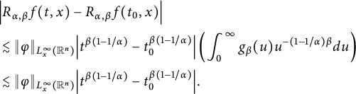 $$ \begin{align} &\Big|R_{\alpha,\beta}f(t,x)-R_{\alpha,\beta}f(t_{0},x)\Big| \\&\lesssim \|\varphi\|_{L^{\infty}_{x}(\mathbb R^{n})}\Big|t^{\beta(1-1/\alpha)}-t_{0}^{\beta(1-1/\alpha)}\Big|\left(\int^{\infty}_{0}g_{\beta}(u)u^{-(1-1/\alpha)\beta}du\right)\nonumber\\ &\lesssim \|\varphi\|_{L^{\infty}_{x}(\mathbb R^{n})}\Big|t^{\beta(1-1/\alpha)}-t_{0}^{\beta(1-1/\alpha)}\Big|.\nonumber \end{align} $$
Now, fix $(t_{0}, x_{0})\in \mathbb R^{1+n}_{+}$
. Since
$(t_{0}, x_{0})\in \mathbb R^{1+n}_{+}$
. Since
 $$ \begin{align*} &\Big|R_{\alpha,\beta}\varphi(t,x)-R_{\alpha,\beta}\varphi(t_{0},x_{0})\Big|\\&\quad\leq \Big|R_{\alpha,\beta}\varphi(t,x)-R_{\alpha,\beta}\varphi(t_{0},x)\Big|+\Big|R_{\alpha,\beta}f(t_{0},x)-R_{\alpha,\beta}\varphi(t_{0},x_{0})\Big|, \end{align*} $$
it follows from (2.11)–(2.13) that
 $$ \begin{align*} \lim_{(t,x)\rightarrow(t_{0},x_{0})}R_{\alpha,\beta}\varphi(t,x)=R_{\alpha,\beta}\varphi(t_{0},x).\\[-42pt] \end{align*} $$
Theorem 2.13 Assume that $(\alpha ,\beta ,p,q)\in (n,\infty )\times (0,1)\times [1,\infty )\times (1,\infty )$
satisfying
$(\alpha ,\beta ,p,q)\in (n,\infty )\times (0,1)\times [1,\infty )\times (1,\infty )$
satisfying $n\beta /p+\alpha /q<\alpha $
. For
$n\beta /p+\alpha /q<\alpha $
. For $g\in L^{q}_{t}L^{p}_{x}(\mathbb R^{1+n}_{+})$
,
$g\in L^{q}_{t}L^{p}_{x}(\mathbb R^{1+n}_{+})$
, $G_{\alpha ,\beta }(g)$
is Hölder continuous in the sense that for any two sufficient close points
$G_{\alpha ,\beta }(g)$
is Hölder continuous in the sense that for any two sufficient close points $(t,x), (t_{0},x_{0})\in \mathbb R^{1+n}_{+}$
,
$(t,x), (t_{0},x_{0})\in \mathbb R^{1+n}_{+}$
,
 $$ \begin{align*} \Big|G_{\alpha,\beta}(g)(t,x)\kern1.1pt{-}\kern1.1pt G_{\alpha,\beta}(t_{0}, x_{0})\Big| \kern1.3pt{\lesssim}\kern1.3pt\|g\|_{L^{q}_{t}L^{p}_{x}(\mathbb R^{n})}\!\left\{|t\kern1.3pt{-}\kern1.3pt t_{0}|^{1-1/q-n\beta/(\alpha p)}\kern1.1pt{+}\kern1.3pt|x\kern1.3pt{-}\kern1.3pt x_{0}|^{\alpha(1-1/q)/\beta-n/p}\kern-1.5pt\right\}\kern-1.2pt. \end{align*} $$
Proof Given a point $(t_{0}, x_{0})\in \mathbb R^{1+n}_{+}$
, let
$(t_{0}, x_{0})\in \mathbb R^{1+n}_{+}$
, let $x\in \mathbb R^{n}$
be sufficiently close to
$x\in \mathbb R^{n}$
be sufficiently close to $x_{0}$
such that
$x_{0}$
such that $\delta =|x-x_{0}|$
small enough. Then
$\delta =|x-x_{0}|$
small enough. Then $|G_{\alpha ,\beta }(g)(t_{0},x)-G_{\alpha ,\beta }(t_{0}, x_{0})|\lesssim I+II,$
where
$|G_{\alpha ,\beta }(g)(t_{0},x)-G_{\alpha ,\beta }(t_{0}, x_{0})|\lesssim I+II,$
where
 $$ \begin{align*}\left\{\begin{aligned} I&:=\int_{0}^{t_{0}}\int_{B(x_{0}, 3\delta)}\Big|G_{t_{0}-s}(x_{0}-y)-G_{t_{0}-s}(x-y)\Big||g(s,y)|dyds,\\ II&:=\int_{0}^{t_{0}}\int_{\mathbb R^{n}\setminus B(x_{0}, 3\delta)}\Big|G_{t_{0}-s}(x_{0}-y)-G_{t_{0}-s}(x-y)\Big||g(s,y)|dyds. \end{aligned}\right.\end{align*} $$
We first estimate I. Write
 $$ \begin{align*} I \lesssim \!\int^{t_{0}}_{0}\!\int_{B(x_{0}, 3\delta)}\kern-1pt\Big|G_{t_{0}-s}(x_{0}-y)\Big||g(s,y)|dyds+\!\int^{t_{0}}_{0}\!\int_{B(x_{0}, 3\delta)}\Big|G_{t_{0}-s}(x-y)\Big||g(s,y)|dyds. \end{align*} $$
We further split
 $$ \begin{align*}\int^{t_{0}}_{0}\int_{B(x_{0}, 3\delta)}\Big|G_{t_{0}-s}(x_{0}-y)\Big||g(s,y)|dyds\lesssim I_{1}+I_{2},\end{align*} $$
where
 $$ \begin{align*}\left\{\begin{aligned} I_{1}&:=\int^{t_{0}-(2\delta)^{\alpha/\beta}}_{0}\int_{B(x_{0}, 3\delta)}\Big|G_{t_{0}-s}(x_{0}-y)\Big||g(s,y)|dyds,\\ I_{2}&:=\int^{t_{0}}_{t_{0}-(2\delta)^{\alpha/\beta}}\int_{B(x_{0}, 3\delta)}\Big|G_{t_{0}-s}(x_{0}-y)\Big||g(s,y)|dyds.\\ \end{aligned}\right.\end{align*} $$
Applying Hölder’s inequality to the variables y and s, respectively, we have
 $$ \begin{align*} I_{1}&\lesssim \int^{t_{0}-(2\delta)^{\alpha/\beta}}_{0}\int_{B(x_{0}, 3\delta)}\frac{|t_{0}-s|^{\beta}}{(|t_{0}-s|^{\beta/\alpha}+|x_{0}-y|)^{n+\alpha}}|g(s,y)|dyds\\ &\lesssim \int^{t_{0}-(2\delta)^{\alpha/\beta}}_{0}\frac{1}{|t_{0}-s|^{\beta n/\alpha}}\Bigg(\int_{B(x_{0}, 3\delta)}|g(y,s)|^{p}dy\Bigg)^{1/p} \Bigg(\int_{B(x_{0}, 3\delta)}1 dy\Bigg)^{1-1/p}ds\\ &\lesssim \int^{t_{0}-(2\delta)^{\alpha/\beta}}_{0}\frac{1}{|t_{0}-s|^{\beta n/\alpha}}\|g(s,\cdot)\|_{L^{p}_{x}(\mathbb R^{n})}\delta^{n(1-1/p)}ds\\ &\lesssim \|g(\cdot,\cdot)\|_{L^{q}_{t}L^{p}_{x}(\mathbb R^{1+n}_{+})}\delta^{\alpha(1-1/q)/\beta-n/p}. \end{align*} $$
Similarly, for $I_{2}$
, we have
$I_{2}$
, we have
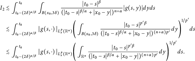 $$ \begin{align*} I_{2}&\lesssim \int^{t_{0}}_{t_{0}-(2\delta)^{\alpha/\beta}}\int_{B(x_{0}, 3\delta)}\frac{|t_{0}-s|^{\beta}}{(|t_{0}-s|^{\beta/\alpha}+|x_{0}-y|)^{n+\alpha}}|g(s,y)|dyds\\ &\lesssim \int^{t_{0}}_{t_{0}-(2\delta)^{\alpha/\beta}}\|g(s,\cdot)\|_{L^{p}_{x}(\mathbb R^{n})}\Bigg(\int_{B(x_{0}, 3\delta)}\frac{|t_{0}-s|^{p'\beta}}{(|t_{0}-s|^{\beta/\alpha}+|x_{0}-y|)^{(n+\alpha)p'}}dy\Bigg)^{1/p'}ds\\ &\lesssim \int^{t_{0}}_{t_{0}-(2\delta)^{\alpha/\beta}}\|g(s,\cdot)\|_{L^{p}_{x}(\mathbb R^{n})}\Bigg(\int_{\mathbb R^{n}}\frac{|t_{0}-s|^{p'\beta}}{(|t_{0}-s|^{\beta/\alpha}+|x_{0}-y|)^{(n+\alpha)p'}}dy\Bigg)^{1/p'}ds. \end{align*} $$
Split
 $$ \begin{align*} &\int_{\mathbb R^{n}}\frac{|t_{0}-s|^{p'\beta}}{(|t_{0}-s|^{\beta/\alpha}+|x_{0}-y|)^{(n+\alpha)p'}}dy\\ &\lesssim \int_{|y-x_{0}|<|t_{0}-s|^{\beta/\alpha}}\frac{|t_{0}-s|^{p'\beta}}{(|t_{0}-s|^{\beta/\alpha}+|x_{0}-y|)^{(n+\alpha)p'}}dy\\ &\quad+\sum^{\infty}_{k=0}\int_{2^{k}|t_{0}-s|^{\beta/\alpha}\leq|y-x_{0}|<2^{k+1}|t_{0}-s|^{\beta/\alpha}} \frac{|t_{0}-s|^{p'\beta}}{(|t_{0}-s|^{\beta/\alpha}+|x_{0}-y|)^{(n+\alpha)p'}}dy\\ &\lesssim \int_{|y-x_{0}|<|t_{0}-s|^{\beta/\alpha}}\frac{|t_{0}-s|^{p'\beta}}{|t_{0}-s|^{\beta(n+\alpha)p'/\alpha}}dy\\ &\quad+\sum^{\infty}_{k=0}\int_{2^{k}|t_{0}-s|^{\beta/\alpha}\leq|y-x_{0}|<2^{k+1}|t_{0}-s|^{\beta/\alpha}} \frac{|t_{0}-s|^{p'\beta}}{(2^{k}|t_{0}-s|^{\beta/\alpha})^{(n+\alpha)p'}}dy\\ &\lesssim \frac{|t_{0}-s|^{p'\beta}}{|t_{0}-s|^{\beta(n+\alpha)p'/\alpha}}|t_{0}-s|^{n\beta/\alpha} +\sum^{\infty}_{k=0}\frac{|t_{0}-s|^{p'\beta}}{(2^{k}|t_{0}-s|)^{\beta(n+\alpha)p'/\alpha}}(2^{k+1}|t_{0}-s|^{\beta/\alpha})^{n}\\ &\lesssim \frac{1}{|t_{0}-s|^{n\beta(p'-1)/\alpha}}. \end{align*} $$
Then we obtain
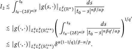 $$ \begin{align*} I_{2}&\lesssim \int^{t_{0}}_{t_{0}-(2\delta)^{\alpha/\beta}}\|g(s,\cdot)\|_{L^{p}_{x}(\mathbb R^{n})}\frac{ds}{|t_{0}-s|^{n\beta/\alpha p}}\\ &\lesssim \|g(\cdot,\cdot)\|_{L^{q}_{t}L^{p}_{x}(\mathbb R^{1+n}_{+})}\Bigg(\int^{t_{0}}_{t_{0}-(2\delta)^{\alpha/\beta}}\frac{ds}{|t_{0}-s|^{n\beta q'/\alpha p}}\Bigg)^{1/q'}\\ &\lesssim \|g(\cdot,\cdot)\|_{L^{q}_{t}L^{p}_{x}(\mathbb R^{1+n}_{+})}\delta^{\alpha(1-1/q)/\beta-n/p}. \end{align*} $$
Now, we estimate $II$
. It follows from (ii) of Proposition 2.9 that there exists a constant
$II$
. It follows from (ii) of Proposition 2.9 that there exists a constant $\epsilon>0$
such that for
$\epsilon>0$
such that for $|x-x_{0}|<|x|/2$
,
$|x-x_{0}|<|x|/2$
,
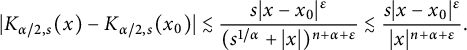 $$ \begin{align*} |K_{\alpha/2,s}(x)-K_{\alpha/2,s}(x_{0})|\lesssim\frac{s|x-x_{0}|^{\epsilon}}{(s^{1/\alpha}+|x|)^{n+\alpha+\epsilon}}\lesssim \frac{s|x-x_{0}|^{\epsilon}}{|x|^{n+\alpha+\epsilon}}. \end{align*} $$
We have
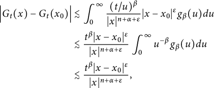 $$ \begin{align*} \Big|G_{t}(x)-G_{t}(x_{0})\Big|&\lesssim \int^{\infty}_{0}\frac{(t/u)^{\beta}}{|x|^{n+\alpha+\epsilon}}|x-x_{0}|^{\epsilon}g_{\beta}(u)du\\ &\lesssim \frac{t^{\beta}|x-x_{0}|^{\epsilon}}{|x|^{n+\alpha+\epsilon}}\int^{\infty}_{0}u^{-\beta}g_{\beta}(u)du\\ &\lesssim \frac{t^{\beta}|x-x_{0}|^{\epsilon}}{|x|^{n+\alpha+\epsilon}}, \end{align*} $$
which implies that
 $$ \begin{align*} \Big|G_{t}(x)-G_{t}(x_{0})\Big|\lesssim\min\left\{\left(\frac{|x-x_{0}|}{t^{\beta/\alpha}}\right)^{\epsilon} \frac{1}{t^{n\beta/\alpha}},\ \frac{t^{\beta}|x-x_{0}|^{\epsilon}}{|x|^{n+\alpha+\epsilon}}\right\}. \end{align*} $$
If $|x|\leq t^{\beta /\alpha }$
, we have
$|x|\leq t^{\beta /\alpha }$
, we have
 $$ \begin{align*} \Big|G_{t}(x)-G_{t}(x_{0})\Big|\lesssim\frac{|x-x_{0}|^{\epsilon}t^{\beta}}{t^{\beta(n+\alpha+\epsilon)/\alpha}}\lesssim \frac{|x-x_{0}|^{\epsilon}t^{\beta}}{(t^{\beta/\alpha}+|x|)^{n+\alpha+\epsilon}}. \end{align*} $$
If $|x|> t^{\beta /\alpha }$
, it still holds
$|x|> t^{\beta /\alpha }$
, it still holds
 $$ \begin{align} \Big|G_{t}(x)-G_{t}(x_{0})\Big|\lesssim\frac{|x-x_{0}|^{\epsilon}t^{\beta}}{|x|^{n+\alpha+\epsilon}}\lesssim \frac{|x-x_{0}|^{\epsilon}t^{\beta}}{(t^{\beta/\alpha}+|x|)^{n+\alpha+\epsilon}}. \end{align} $$
Applying (2.14), we can deduce that
 $$ \begin{align*} II&\lesssim \int^{t_{0}}_{0}\int_{\mathbb R^{n}\setminus B(x_{0}, 3\delta)}\frac{\delta^{\epsilon}|t_{0}-s|^{\beta}}{(|t_{0}-s|^{\beta/\alpha}+|x_{0}-y|)^{n+\alpha+\epsilon}}|g(s,y)|dyds\\ &\lesssim \int^{t_{0}-(2\delta)^{\alpha/\beta}}_{0}\int_{\mathbb R^{n}\setminus B(x_{0}, 3\delta)}\frac{\delta^{\epsilon}|t_{0}-s|^{\beta}}{(|t_{0}-s|^{\beta/\alpha}+|x_{0}-y|)^{n+\alpha+\epsilon}}|g(s,y)|dyds\\ &\quad +\int^{t_{0}}_{t_{0}-(2\delta)^{\alpha/\beta}}\int_{\mathbb R^{n}\setminus B(x_{0}, 3\delta)}\frac{\delta^{\epsilon}|t_{0}-s|^{\beta}}{(|t_{0}-s|^{\beta/\alpha}+|x_{0}-y|)^{n+\alpha+\epsilon}}|g(s,y)|dyds\\ &:= II_{1}+II_{2}, \end{align*} $$
where
 $$ \begin{align*} II_{1}&\lesssim \int^{t_{0}-(2\delta)^{\alpha/\beta}}_{0}\int_{\mathbb R^{n}\setminus B(x_{0}, 3\delta)}\frac{\delta^{\epsilon}|t_{0}-s|^{\beta}}{(|t_{0}-s|^{\beta/\alpha}+|x_{0}-y|)^{n+\alpha+\epsilon}}|g(s,y)|dyds\\ &\lesssim \int^{t_{0}-(2\delta)^{\alpha/\beta}}_{0}\!\delta^{\epsilon}|t_{0}-s|^{\beta}\|g(s,\cdot)\|_{L^{p}_{x}(\mathbb R^{n})}\Bigg(\kern-2pt\int_{\mathbb R^{n}\setminus B(x_{0}, 3\delta)} \!\frac{dy}{(|t_{0}-s|^{\beta/\alpha}+|x_{0}-y|)^{p'(n+\alpha+\epsilon)}}\kern-1pt\Bigg)^{\kern-0.1pt1/p'}ds \end{align*} $$
and, similarly,
 $$ \begin{align*} II_{2} \lesssim \int_{t_{0}-(2\delta)^{\alpha/\beta}}^{t_0}\delta^{\epsilon}|t_{0}-s|^{\beta}\|g(s,\cdot)\|_{L^{p}_{x} (\mathbb R^{n})}\Bigg(\int_{\mathbb R^{n}\setminus B(x_{0}, 3\delta)}\frac{dy}{|x_{0}-y|^{p'(n+\alpha+\epsilon)}}\Bigg)^{1/p'}ds. \end{align*} $$
We first estimate $II_{1}$
. The following integral can be estimated as
$II_{1}$
. The following integral can be estimated as
 $$ \begin{align*} \int_{\mathbb R^{n}\setminus B(x_{0}, 3\delta)}\frac{\delta^{p'\epsilon}|t_{0}-s|^{p'\beta}dy}{(|t_{0}-s|^{\beta/\alpha}+|x_{0}-y|)^{p'(n+\alpha+\epsilon)}} &\lesssim \sum^{\infty}_{j=1}\frac{\delta^{p'\epsilon}|t_{0}-s|^{p'\beta}(3^{j}\delta)^{n}} {(|t_{0}-s|^{\beta/\alpha}+3^{j}\delta)^{p'(n+\alpha+\epsilon)}}\\ &\lesssim \sum^{\infty}_{j=1}\frac{1}{3^{j}}\int^{3^{j+1}\delta}_{3^{j}\delta} \frac{\delta^{p'\epsilon-1}|t_{0}-s|^{p'\beta}}{(|t_{0}-s|^{\beta/\alpha}+r)^{p'(n+\alpha+\epsilon)-n}}dr\\ &\lesssim \int^{\infty}_{3\delta} \frac{\delta^{p'\epsilon-1}|t_{0}-s|^{p'\beta}}{(|t_{0}-s|^{\beta/\alpha}+r)^{p'(n+\alpha+\epsilon)-n}}dr. \end{align*} $$
A direct computation gives
 $$ \begin{align*} \int^{\infty}_{3\delta} \frac{\delta^{p'\epsilon-1}|t_{0}-s|^{p'\beta}}{(|t_{0}-s|^{\beta/\alpha}+r)^{p'(n+\alpha+\epsilon)-n}}dr &\lesssim \delta^{p'\epsilon-1}|t_{0}-s|^{p'\beta}\int^{\infty}_{3\delta+|t_{0}-s|^{\beta/\alpha}} \frac{1}{u^{p'(n+\alpha+\epsilon)-n}}du\\ &\lesssim \frac{\delta^{p'\epsilon-\beta}|t_{0}-s|^{p'\beta}}{(3\delta+|t_{0}-s|^{\beta/\alpha})^{p'(n+\alpha+\epsilon)-n-1}}, \end{align*} $$
which yields
 $$ \begin{align*} II_{1}&\lesssim \int^{t_{0}-(2\delta)^{\alpha/\beta}}_{0}\|g(s,\cdot)\|_{L^{p}_{x}(\mathbb R^{n})} \frac{\delta^{\epsilon-1/p'}|t_{0}-s|^{\beta}}{(\delta+|t_{0}-s|^{\beta/\alpha})^{(n+\alpha+\epsilon)-(n+1)/p'}}ds\\ &\lesssim \int^{t_{0}-(2\delta)^{\alpha/\beta}}_{0}\|g(s,\cdot)\|_{L^{p}_{x}(\mathbb R^{n})} \frac{\delta^{\epsilon-1/p'}}{(\delta+|t_{0}-s|^{\beta/\alpha})^{n/p+\epsilon-1/p'}}ds\\ &\lesssim \delta^{\epsilon-1/p'}\|g\|_{L^{q}_{t}L^{p}_{x}(\mathbb R^{1+n}_{+})}\Bigg(\int^{t_{0}-(2\delta)^{\alpha}}_{0}\frac{1}{(\delta+|t_{0}-s|^{\beta/\alpha})^{(n/p+\epsilon-1/p')q'}}ds\Bigg)^{1/q'}\\ &\lesssim \delta^{\alpha(1-1/q)/\beta-n/p}\|g\|_{L^{q}_{t}L^{p}_{x}(\mathbb R^{1+n}_{+})}. \end{align*} $$
For the term $II_{2}$
, an application of Hölder’s inequality yields
$II_{2}$
, an application of Hölder’s inequality yields
 $$ \begin{align*} II_{2}&\lesssim \int^{t_{0}}_{t_{0}-(2\delta)^{\alpha/\beta}}|t_{0}-s|^{\beta}\delta^{\epsilon} \|g(s,\cdot)\|_{L^{p}_{x}(\mathbb R^{n})}\Bigg(\int_{\mathbb R^{n}\setminus B(x_{0},3\delta)}\frac{dy}{|x_{0}-y|^{p'(n+\epsilon+\alpha)}}\Bigg)^{p'}ds\\ &\lesssim \int^{t_{0}}_{t_{0}-(2\delta)^{\alpha/\beta}}\|g(s,\cdot)\|_{L^{p}_{x}(\mathbb R^{n})}|t_{0}-s|^{\beta}\delta^{-(n+\epsilon+\alpha)+n/p'}\delta^{\epsilon}ds\\ &\lesssim \delta^{-(n+\epsilon+\alpha)+n/p'}\delta^{\epsilon}\|g\|_{L^{q}_{t}L^{p}_{x}(\mathbb R^{1+n}_{+})}\Bigg(\int^{t_{0}}_{t_{0}-(2\delta)^{\alpha/\beta}}|t_{0}-s|^{\beta q'}ds\Bigg)^{1/q'}\\ &\lesssim \|g\|_{L^{q}_{t}L^{p}_{x}(\mathbb R^{1+n}_{+})}\delta^{\alpha(1-1/q)/\beta-n/p}. \end{align*} $$
The estimates for I and $II$
imply that
$II$
imply that
 $$ \begin{align*} \Big|G_{\alpha,\beta}(g)(t_{0},x_{0})-G_{\alpha,\beta}(g)(t_{0},x)\Big| \lesssim \|g\|_{L^{q}_{t}L^{p}_{x}(\mathbb R^{1+n}_{+})}\delta^{\alpha(1-1/q)/\beta-n/p}. \end{align*} $$
For fixed $x\in \mathbb R^{n}$
and
$x\in \mathbb R^{n}$
and $t_{1}>t_{2}$
, we can see that
$t_{1}>t_{2}$
, we can see that
 $$ \begin{align*} \Big|G_{\alpha,\beta}(g)(t_{1},x)-G_{\alpha,\beta}(g)(t_{2},x)\Big|\lesssim III+IV, \end{align*} $$
where
 $$ \begin{align*}\left\{\begin{aligned} III&:=\Bigg|\int^{t_{2}}_{0}\int_{\mathbb R^{n}}\left(G_{t_{1}-s}(x-y)-G_{t_{2}-s}(x-y)\right)g(s,y)dsdy\Bigg|,\\ IV&:=\Bigg|\int^{t_{1}}_{t_{2}}\int_{\mathbb R^{n}}G_{t_{1}-s}(x-y)g(s,y)dyds\Bigg|. \end{aligned}\right.\end{align*} $$
It follows from Hölder’s inequality that
 $$ \begin{align*} IV&\lesssim \int^{t_{1}}_{t_{2}}\int_{\mathbb R^{n}}|G_{t_{1}-s}(x-y)||g(s,y)|dyds\\ &\lesssim \int^{t_{1}}_{t_{2}}\|g(s,\cdot)\|_{L^{p}_{x}(\mathbb R^{n})}\left\{\int_{\mathbb R^{n}}\frac{|t_{1}-s|^{\beta p'}}{(|t_{1}-s|^{\beta/\alpha}+|x-y|)^{(n+\alpha)p'}}dy\right\}^{1/p'}ds\\ &\lesssim \int^{t_{1}}_{t_{2}}\|g(s,\cdot)\|_{L^{p}_{x}(\mathbb R^{n})}|t_{1}-s|^{-\beta n/(\alpha p)}ds\\ &\lesssim \|g\|_{L^{q}_{t}L^{p}_{x}(\mathbb R^{1+n}_{+})}\Bigg(\int^{t_{1}}_{t_{2}}|t_{1}-s|^{-\beta nq'/(\alpha p)}ds\Bigg)^{1/q'}\\ &\lesssim \|g\|_{L^{q}_{t}L^{p}_{x}(\mathbb R^{1+n}_{+})}|t_{1}-t_{2}|^{1-1/q-n\beta/(\alpha p)}. \end{align*} $$
To estimate $III$
, we first investigate the Lipschitz continuity of
$III$
, we first investigate the Lipschitz continuity of $G_{t}(\cdot )$
on the time variable t. Because
$G_{t}(\cdot )$
on the time variable t. Because
 $$ \begin{align*} G_{t_{1}-s}(x-y)-G_{t_{2}-s}(x-y) = \!\int^{\infty}_{0}\!\left(K_{\alpha,\left(\frac{t_{1}-s}{u}\right)^{\beta}} (x-y)-K_{\alpha,\left(\frac{t_{2}-s}{u}\right)^{\beta}}(x-y)\kern-1pt\right) g_{\beta}(u)du, \end{align*} $$
it holds
 $$ \begin{align*} III&= \Bigg|\int^{t_{2}}_{0}\int_{\mathbb R^{n}}\left\{\int^{\infty}_{0}\left(K_{\alpha/2,\left(\frac{t_{1}-s}{u}\right)^{\beta}}(x-y)-K_{\alpha/2,\left(\frac{t_{2}-s}{u}\right)^{\beta}}(x-y)\right)g_{\beta}(u)du\right\} g(s,y)dsdy\Bigg|\\ &= \Bigg|\int^{t_{2}}_{0}\int^{\infty}_{0}\left\{\int_{\mathbb R^{n}}\left(K_{\alpha/2,\left(\frac{t_{1}-s}{u}\right)^{\beta}}(x-y)-K_{\alpha/2,\left(\frac{t_{2}-s}{u}\right)^{\beta}}(x-y)\right)g(s,y)dy\right\}g_{\beta}(u)dsdu\Bigg|\\ &= \Bigg|\int^{\infty}_{0}\int^{t_{2}}_{0}\Bigg\{e^{-\left(\frac{t_{1}-s}{u}\right)^{\beta}(-\Delta)^{\alpha/2}}(\varphi)(s,x)- e^{-\left(\frac{t_{2}-s}{u}\right)^{\beta}(-\Delta)^{\alpha/2}}(\varphi)(s,x)\Bigg\}g_{\beta}(u)dsdu\Bigg|. \end{align*} $$
Noticing that
 $$ \begin{align*} &\left|e^{-\left(\frac{t_{1}-s}{u}\right)^{\beta}(-\Delta)^{\alpha/2}}(\varphi)(s,x)- e^{-\left(\frac{t_{2}-s}{u}\right)^{\beta}(-\Delta)^{\alpha/2}} (\varphi)(s,x)\right|\\ &\quad= \left|\int^{\left(\frac{t_{1}-s}{u}\right)^{\beta}}_{\left(\frac{t_{2}-s}{u}\right)^{\beta}} \frac{\partial}{\partial_{r}}e^{-r(-\Delta)^{\alpha/2}}(\varphi)(s,x)dr\right|\\ &\quad\lesssim \int^{\left(\frac{t_{1}-s}{u}\right)^{\beta}}_{\left(\frac{t_{2}-s}{u}\right)^{\beta}} \left|(-\Delta)^{\alpha/2} e^{-r(-\Delta)^{\alpha/2}}(\varphi)(s,x)\right|dr\\ &\quad\lesssim \int^{\left(\frac{t_{1}-s}{u}\right)^{\beta}}_{\left(\frac{t_{2}-s}{u}\right)^{\beta}}r^{-1-n/(\alpha p)}\|g(s,\cdot)\|_{L^{p}_{x}(\mathbb R^{n})}dr, \end{align*} $$
we can obtain
 $$ \begin{align*} III&\lesssim \int^{\infty}_{0}\left\{\int^{t_{2}}_{0} \left(\int^{\left(\frac{t_{1}-s}{u}\right)^{\beta}}_{\left(\frac{t_{2}-s}{u}\right)^{\beta}}r^{-1-\frac{n}{\alpha p}}\|g(s,\cdot)\|_{L^{p}_{x}(\mathbb R^{n})}dr\right)ds\right\}g_{\beta}(u)du\\ &\lesssim \int^{\infty}_{0}\left\{\int^{t_{2}}_{0}\left(\int^{\left(\frac{t_{1}-s}{u}\right)^{\beta}}_{\left(\frac{t_{2}-s}{u}\right)^{\beta}}r^{-1-\frac{n}{\alpha p}}dr\right)\|g(s,\cdot)\|_{L^{p}_{x}(\mathbb R^{n})}ds\right\}g_{\beta}(u)du\\ &\lesssim \int^{\infty}_{0}\left\{\int^{t_{2}}_{0}\left(\int^{\left(\frac{t_{1}-s}{u}\right)^{\beta}- \left(\frac{t_{2}-s}{u}\right)^{\beta}}_{0} \frac{dr}{\left(r+\left(\frac{t_{2}-s}{u}\right)^{\beta}\right)^{1+\frac{n}{\alpha p}}}\right)\|g(s,\cdot)\|_{L^{p}_{x}(\mathbb R^{n})}ds\right\}g_{\beta}(u)du. \end{align*} $$
Since for $\beta \in (0,1)$
,
$\beta \in (0,1)$
,
 $$ \begin{align*} (t_{1}/u-s/u)^{\beta}-(t_{2}/u-s/u)^{\beta}\leq \left(t_{1}/u-t_{2}/{u}\right)^{\beta}, \end{align*} $$
applying Fubini’s theorem and Hölder’s inequality, we can get
 $$ \begin{align*} III&\lesssim \int^{\infty}_{0}\Bigg\{\int^{t_{2}}_{0}\left(\int^{(\frac{t_{1}-t_{2}}{u})^{\beta}}_{0}\frac{dr}{\left(r+\left(\frac{t_{2}-s}{u}\right)^{\beta}\right)^{1+\frac{n}{\alpha p}}}\right)\|g(s,\cdot)\|_{L^{p}_{x}(\mathbb R^{n})}ds\Bigg\}g_{\beta}(u)du\\ &\lesssim \int^{\infty}_{0}\left\{\int^{(\frac{t_{1}-t_{2}}{u})^{\beta}}_{0}\left(\int^{t_{2}}_{0}\frac{\|g(s,\cdot)\|_{L^{p}_{x}(\mathbb R^{n})}}{\left(r+\left(\frac{t_{2}-s}{u}\right)^{\beta}\right)^{1+\frac{n}{\alpha p}}}ds\right)dr\right\}g_{\beta}(u)du\\ &\lesssim \|g\|_{L^{q}_{t}L^{p}_{x}(\mathbb R^{1+n}_{+})}\int^{\infty}_{0}\Bigg\{\int^{(\frac{t_{1}-t_{2}}{u})^{\beta}}_{0} \Bigg(\int^{t_{2}}_{0}\frac{ds}{\left(r+\left(\frac{t_{2}-s}{u}\right)^{\beta}\right)^{(1+\frac{n}{\alpha p})q'}}\Bigg)^{1/q'}dr\Bigg\}g_{\beta}(u)du. \end{align*} $$
By change of variables, we obtain
 $$ \begin{align*} \int^{t_{2}}_{0}\frac{ds}{\left(r+\left(\frac{t_{2}-s}{u}\right)^{\beta}\right)^{(1+\frac{n}{\alpha p})q'}} = u\int^{(t_{2}/u)^{\beta}}_{0}\frac{s^{1/\beta-1}_{1}ds_{1}}{(r+s_{1})^{(1+\frac{n}{\alpha p})q'}} \lesssim u r^{-(1+\frac{n}{\alpha p})q'+\frac{1}{\beta}}. \end{align*} $$
Finally, we have, upon $1/q'\beta -n/(\alpha p)>0$
,
$1/q'\beta -n/(\alpha p)>0$
,
 $$ \begin{align*} III&\lesssim \|g\|_{L^{q}_{t}L^{p}_{x}(\mathbb R^{1+n}_{+})}\int^{\infty}_{0}\Bigg\{\int^{(t_{1}/u-t_{2}/u)^{\beta}}_{0} r^{-(1+\frac{n}{\alpha p})+\frac{1}{q'\beta}}dr\Bigg\}u^{1/q'}g_{\beta}(u)du\\ &\lesssim \|g\|_{L^{q}_{t}L^{p}_{x}(\mathbb R^{1+n}_{+})}\int^{\infty}_{0}\left(\frac{t_{1}-t_{2}}{u}\right)^{(\frac{1}{q'}-\frac{\beta n}{\alpha p})}u^{1/q'}g_{\beta}(u)du\\ &\lesssim \|g\|_{L^{q}_{t}L^{p}_{x}(\mathbb R^{1+n}_{+})}|t_{1}-t_{2}|^{1-1/q-n\beta/(\alpha p)}, \end{align*} $$
where in the last inequality we have used the following estimate: $\int ^{\infty }_{0}u^{\beta n/\alpha p}g_{\beta }(u)du<\infty $
. In fact, by (2.2),
$\int ^{\infty }_{0}u^{\beta n/\alpha p}g_{\beta }(u)du<\infty $
. In fact, by (2.2), $g_{\beta }(u)\lesssim u^{(N\beta -1+\beta /2)/(1-\beta )}$
for
$g_{\beta }(u)\lesssim u^{(N\beta -1+\beta /2)/(1-\beta )}$
for $u\in (0,1)$
and N being large enough, which indicates that
$u\in (0,1)$
and N being large enough, which indicates that
 $$ \begin{align*} \int^{1}_{0}u^{\beta n/\alpha p}g_{\beta}(u)du \lesssim\int^{1}_{0}u^{\beta n/\alpha p}u^{(N\beta-1+\beta/2)/(1-\beta)}du<\infty. \end{align*} $$
On the other hand, under the assumption that $\alpha>n$
and
$\alpha>n$
and $\beta \in (0,1)$
, we can see that
$\beta \in (0,1)$
, we can see that $\beta n/(\alpha p)-\beta -1<-1 $
and therefore
$\beta n/(\alpha p)-\beta -1<-1 $
and therefore
 $$ \begin{align*} \int^{\infty}_{1}u^{\beta n/(\alpha p)}g_{\beta}(u)du\lesssim\int^{\infty}_{1}u^{\beta n/(\alpha p)}u^{-\beta-1}du<\infty.\\[-42pt] \end{align*} $$
Theorems 2.12 and 2.13 show that, for the case $\alpha (1-1/q)-\beta n/p>0$
, the solution for (1.2) is continuous. For the endpoint case
$\alpha (1-1/q)-\beta n/p>0$
, the solution for (1.2) is continuous. For the endpoint case $\alpha (1-1/q)-\beta n/p=0$
, we can obtain the following Moser–Trudinger-type estimate for
$\alpha (1-1/q)-\beta n/p=0$
, we can obtain the following Moser–Trudinger-type estimate for $G_{\alpha ,\beta }$
.
$G_{\alpha ,\beta }$
.
Theorem 2.14 Given $\alpha>n$
and
$\alpha>n$
and $0<\beta <1$
. Assume that
$0<\beta <1$
. Assume that $p\in [1,\infty )$
,
$p\in [1,\infty )$
, $1<q<\infty $
, and
$1<q<\infty $
, and $n\beta /(\alpha p)+1/q=1$
. Let
$n\beta /(\alpha p)+1/q=1$
. Let $(t_{0}, x_{0})\in \mathbb R^{1+n}_{+}$
,
$(t_{0}, x_{0})\in \mathbb R^{1+n}_{+}$
, $r_{0}=t_{0}^{1/(2\alpha )}$
, and
$r_{0}=t_{0}^{1/(2\alpha )}$
, and $0<\|g\|_{L^{q}_{t}L^{p}_{x}(\mathbb R^{1+n}_{+})}$
. There exists a constant
$0<\|g\|_{L^{q}_{t}L^{p}_{x}(\mathbb R^{1+n}_{+})}$
. There exists a constant $C>0$
such that
$C>0$
such that
 $$ \begin{align*} \frac{1}{r^{2\alpha}|B^{(\alpha)}_{r_{0}}(t_{0},x_{0})|}\iint_{B^{(\alpha)}_{r_{0}}(t_{0},x_{0})} \exp\left(\frac{G_{\alpha,\beta}(g)(t,x)}{C\|g\|_{L^{q}_{t}L^{p}_{x}(\mathbb R^{1+n}_{+})}}\right)^{q/(q-1)}dxdt\lesssim1. \end{align*} $$
Proof Let $(t,x)\in \mathbb R^{1+n}_{+}$
be fixed. Then
$(t,x)\in \mathbb R^{1+n}_{+}$
be fixed. Then $|G_{\alpha ,\beta }(g)(t,x)|\lesssim I+II,$
where
$|G_{\alpha ,\beta }(g)(t,x)|\lesssim I+II,$
where
 $$ \begin{align*}\left\{\begin{aligned} I:=\int^{r}_{0}\int_{\mathbb R^{n}}G_{t-s}(x-y)|g(s,y)|dyds,\\ II:=\int^{t}_{r}\int_{\mathbb R^{n}}G_{t-s}(x-y)|g(s,y)|dyds. \end{aligned}\right.\end{align*} $$
Below, we deal with the terms I and $II$
, separately. By Hölder’s inequality, we get
$II$
, separately. By Hölder’s inequality, we get
 $$ \begin{align*} I&\lesssim \int^{r}_{0}\int_{\mathbb R^{n}}\frac{(t-s)^{\beta}}{(|t-s|^{\beta/\alpha}+|x-y|)^{n+\alpha}}g(s,y)dyds\\ &\lesssim \int^{r}_{0}(t-s)^{\beta}\|g(s,\cdot)\|_{L^{p}_{x}(\mathbb R^{n})}\left\{\int_{\mathbb R^{n}}\frac{dy}{(|t-s|^{\beta/\alpha}+|x-y|)^{p(n+\alpha)/(p-1)}}\right\}^{1-1/p}ds. \end{align*} $$
It can be deduced from the integral
 $$ \begin{align*} \int_{\mathbb R^{n}}\frac{dy}{(|t-s|^{\beta/\alpha}+|x-y|)^{p(n+\alpha)/(p-1)}} \lesssim\frac{|t-s|^{n\beta/\alpha}}{|t-s|^{\beta(n/\alpha+1)p/(p-1)}} \end{align*} $$
that
 $$ \begin{align*} I \lesssim \int^{r}_{0}(t-s)^{\beta}\|g(s,\cdot)\|_{L^{p}_{x}(\mathbb R^{n})}\frac{|t-s|^{n\beta (1-/p)/\alpha}}{|t-s|^{\beta(n+\alpha)/\alpha}}ds \lesssim\int^{r}_{0}\|g(s,\cdot)\|_{L^{p}_{x}(\mathbb R^{n})}\frac{ds}{|t-s|^{n\beta/(\alpha p)}}. \end{align*} $$
By the fact that $1/q+n\beta /(\alpha p)=1$
, we apply Hölder’s inequality on s to obtain
$1/q+n\beta /(\alpha p)=1$
, we apply Hölder’s inequality on s to obtain
 $$ \begin{align*} I \lesssim \|g\|_{L^{q}_{t}L^{p}_{x}(\mathbb R^{1+n}_{+})}\left(\int^{r}_{0}\frac{ds}{|t-s|^{n\beta q'/(\alpha p)}}\right)^{1-1/q} \lesssim\|g\|_{L^{q}_{t}L^{p}_{x}(\mathbb R^{1+n}_{+})}\left(\ln\frac{t}{t-r}\right)^{1-1/q}. \end{align*} $$
Denote by $M_{\mathbb R}$
the Hardy–Littlewood maximal function on
$M_{\mathbb R}$
the Hardy–Littlewood maximal function on $\mathbb R$
. Then, since
$\mathbb R$
. Then, since $1-n\beta /(p\alpha )=1/q$
, it holds
$1-n\beta /(p\alpha )=1/q$
, it holds
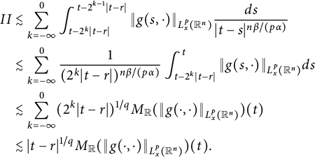 $$ \begin{align*} II&\lesssim \sum^{0}_{k=-\infty}\int^{t-2^{k-1}|t-r|}_{t-2^{k}|t-r|}\|g(s,\cdot)\|_{L^{p}_{x}(\mathbb R^{n})}\frac{ds}{|t-s|^{n\beta/(p\alpha)}}\\ &\lesssim \sum^{0}_{k=-\infty} \frac{1}{(2^{k}|t-r|)^{n\beta/(p\alpha)}}\int^{t}_{t-2^{k}|t-r|}\|g(s,\cdot)\|_{L^{p}_{x}(\mathbb R^{n})}ds\\ &\lesssim\sum^{0}_{k=-\infty}(2^{k}|t-r|)^{1/q}M_{\mathbb R}(\|g(\cdot,\cdot)\|_{L^{p}_{x}(\mathbb R^{n})})(t)\\ &\lesssim|t-r|^{1/q}M_{\mathbb R}(\|g(\cdot,\cdot)\|_{L^{p}_{x}(\mathbb R^{n})})(t). \end{align*} $$
The estimates for I and $II$
indicate that
$II$
indicate that
 $$ \begin{align*}|G_{\alpha,\beta}(g)(t,x)|\lesssim \|g\|_{L^{q}_{t}L^{p}_{x}(\mathbb R^{1+n}_{+})}\left(\ln\frac{t}{t-r}\right)^{1-1/q}+|t-r|^{1/q}M_{\mathbb R}(\|g(\cdot,\cdot)\|_{L^{p}_{x}(\mathbb R^{n})})(t).\end{align*} $$
Via choosing $r\in (0,t)$
such that
$r\in (0,t)$
such that
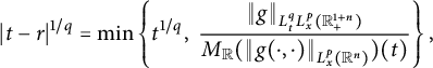 $$ \begin{align*}|t-r|^{1/q}=\min\left\{t^{1/q},\ \frac{\|g\|_{L^{q}_{t}L^{p}_{x}(\mathbb R^{1+n}_{+})}}{M_{\mathbb R}(\|g(\cdot,\cdot)\|_{L^{p}_{x}(\mathbb R^{n})})(t)}\right\}, \end{align*} $$
we get
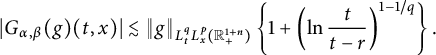 $$ \begin{align*}|G_{\alpha,\beta}(g)(t,x)|\lesssim \|g\|_{L^{q}_{t}L^{p}_{x}(\mathbb R^{1+n}_{+})}\left\{1+\left(\ln\frac{t}{t-r}\right)^{1-1/q}\right\}. \end{align*} $$
Case 1: $|t-r|^{1/q}=t^{1/q}$
. Then
$|t-r|^{1/q}=t^{1/q}$
. Then
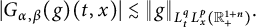 $$ \begin{align*}|G_{\alpha,\beta}(g)(t,x)|\lesssim \|g\|_{L^{q}_{t}L^{p}_{x}(\mathbb R^{1+n}_{+})}.\end{align*} $$
Case 2: $|t-r|^{1/q}=\|g\|_{L^{q}_{t}L^{p}_{x}(\mathbb R^{1+n}_{+})}M^{-1}_{\mathbb R}(\|g(\cdot ,\cdot )\|_{L^{p}_{x}(\mathbb R^{n})})(t)$
. We have
$|t-r|^{1/q}=\|g\|_{L^{q}_{t}L^{p}_{x}(\mathbb R^{1+n}_{+})}M^{-1}_{\mathbb R}(\|g(\cdot ,\cdot )\|_{L^{p}_{x}(\mathbb R^{n})})(t)$
. We have
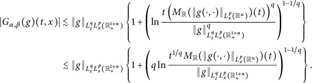 $$ \begin{align*} |G_{\alpha,\beta}(g)(t,x)|&\lesssim \|g\|_{L^{q}_{t}L^{p}_{x}(\mathbb R^{1+n}_{+})}\left\{1+\left(\ln\frac{t\left(M_{\mathbb R}(\|g(\cdot,\cdot)\|_{L^{p}_{x}(\mathbb R^{n})})(t)\right)^{q}}{\|g\|^{q}_{L^{q}_{t}L^{p}_{x}(\mathbb R^{1+n}_{+})}}\right)^{1-1/q}\right\}\\ &\lesssim \|g\|_{L^{q}_{t}L^{p}_{x}(\mathbb R^{1+n}_{+})}\left\{1+\left(q\ln\frac{t^{1/q}M_{\mathbb R}(\|g(\cdot,\cdot)\|_{L^{p}_{x}(\mathbb R^{n})})(t)}{\|g\|_{L^{q}_{t}L^{p}_{x}(\mathbb R^{1+n}_{+})}}\right)^{1-1/q}\right\}. \end{align*} $$
Let $r_{0}=t_{0}^{1/2\alpha }$
. Then
$r_{0}=t_{0}^{1/2\alpha }$
. Then
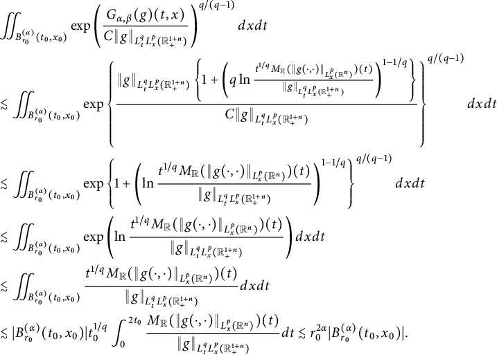 $$ \begin{align*} &\iint_{B^{(\alpha)}_{r_{0}}(t_{0},x_{0})} \exp\left(\frac{G_{\alpha,\beta}(g)(t,x)}{C\|g\|_{L^{q}_{t}L^{p}_{x}(\mathbb R^{1+n}_{+})}}\right)^{q/(q-1)}dxdt\\ &\lesssim \iint_{B^{(\alpha)}_{r_{0}}(t_{0},x_{0})} \exp\left\{\frac{\|g\|_{L^{q}_{t}L^{p}_{x}(\mathbb R^{1+n}_{+})}\left\{1+\left(q\ln\frac{t^{1/q}M_{\mathbb R}(\|g(\cdot,\cdot)\|_{L^{p}_{x}(\mathbb R^{n})})(t)}{\|g\|_{L^{q}_{t}L^{p}_{x}(\mathbb R^{1+n}_{+})}}\right)^{1-1/q}\right\}}{C\|g\|_{{L^{q}_{t}L^{p}_{x}(\mathbb R^{1+n}_{+})}}}\right\}^{q/(q-1)}dxdt\\ &\lesssim \iint_{B^{(\alpha)}_{r_{0}}(t_{0},x_{0})}\exp\left\{1+\left(\ln\frac{t^{1/q}M_{\mathbb R}(\|g(\cdot,\cdot)\|_{L^{p}_{x}(\mathbb R^{n})})(t)}{\|g\|_{L^{q}_{t}L^{p}_{x}(\mathbb R^{1+n}_{+})}}\right)^{1-1/q}\right\}^{q/(q-1)}dxdt\\ &\lesssim \iint_{B^{(\alpha)}_{r_{0}}(t_{0},x_{0})}\exp \left(\ln\frac{t^{1/q}M_{\mathbb R}(\|g(\cdot,\cdot)\|_{L^{p}_{x}(\mathbb R^{n})})(t)}{\|g\|_{L^{q}_{t}L^{p}_{x}(\mathbb R^{1+n}_{+})}}\right)dxdt\\ &\lesssim \iint_{B^{(\alpha)}_{r_{0}}(t_{0},x_{0})}\frac{t^{1/q}M_{\mathbb R}(\|g(\cdot,\cdot)\|_{L^{p}_{x}(\mathbb R^{n})})(t)}{\|g\|_{L^{q}_{t}L^{p}_{x}(\mathbb R^{1+n}_{+})}}dxdt\\ &\lesssim|B^{(\alpha)}_{r_{0}}(t_{0},x_{0})|t^{1/q}_{0}\int^{2t_{0}}_{0}\frac{M_{\mathbb R}(\|g(\cdot,\cdot)\|_{L^{p}_{x}(\mathbb R^{n})})(t)}{\|g\|_{L^{q}_{t}L^{p}_{x}(\mathbb R^{1+n}_{+})}}dt \lesssim r^{2\alpha}_{0}|B^{(\alpha)}_{r_{0}}(t_{0},x_{0})|. \end{align*} $$
This completes the proof of Theorem 2.14.
3
$L^{q}_{t}L^p_{x}$
-capacities associated with space–time fractional equations

In this section, we study the $L^{q}_{t}L^p_{x}$
-capacity associated with
$L^{q}_{t}L^p_{x}$
-capacity associated with $G_{\alpha ,\beta }$
defined in Definition 1.1. We establish the dual form, some basic properties, and the
$G_{\alpha ,\beta }$
defined in Definition 1.1. We establish the dual form, some basic properties, and the $L^{q}_{t}L^p_{x}$
-capacity of fractional parabolic balls in
$L^{q}_{t}L^p_{x}$
-capacity of fractional parabolic balls in $\mathbb {R}^{n+1}_+.$
As a by-product, a strong-type inequality is also obtained.
$\mathbb {R}^{n+1}_+.$
As a by-product, a strong-type inequality is also obtained.
3.1 The dual form of the
$L^{q}_{t}L^p_{x}$
-capacity

First, let us introduce the adjoint operator of $G_{\alpha ,\beta }.$
For any
$G_{\alpha ,\beta }.$
For any $f, g\in C^{\infty }_{0}(\mathbb R^{1+n}_{+})$
, since
$f, g\in C^{\infty }_{0}(\mathbb R^{1+n}_{+})$
, since
 $$ \begin{align*} &\iint_{\mathbb R^{1+n}_{+}}G_{\alpha,\beta}(f)(t,x)g(t,x)dxdt \\&\quad= \iint_{\mathbb R^{1+n}_{+}}\Bigg(\int^{t}_{0}\int_{\mathbb R^{n}}G_{t-s}(x-y)f(s,y)dyds\Bigg)g(t,x)dxdt\\ &\quad= \int^{\infty}_{0}\int_{\mathbb R^{n}}\Bigg(\int^{t}_{0}\int_{\mathbb R^{n}}G_{t-s}(x-y)f(s,y)dyds\Bigg)g(t,x)dxdt\\ &\quad= \int^{\infty}_{0}\int_{\mathbb R^{n}}f(t,x)\Bigg(\int^{\infty}_{t}\int_{\mathbb R^{n}}G_{s-t}(y-x)g(s,y)dsdy\Bigg)dxdt, \end{align*} $$
the adjoint operator $G^{\ast }_{\alpha ,\beta }$
of
$G^{\ast }_{\alpha ,\beta }$
of $G_{\alpha ,\beta }$
is defined via
$G_{\alpha ,\beta }$
is defined via
 $$ \begin{align} G^{\ast}_{\alpha,\beta}(g)(t,x):=\int^{\infty}_{t}\int_{\mathbb R^{n}}G_{s-t}(y-x)g(s,y)dyds. \end{align} $$
The definition of $G^{\ast }_{\alpha ,\beta }$
can be extended to the family of Borel measures
$G^{\ast }_{\alpha ,\beta }$
can be extended to the family of Borel measures $\mu $
with compact supports in
$\mu $
with compact supports in $\mathbb R^{1+n}_{+}$
. Let
$\mathbb R^{1+n}_{+}$
. Let $\|\mu \|_{1}$
denote the total variants of
$\|\mu \|_{1}$
denote the total variants of $\mu $
. If F is continuous and compactly supported in
$\mu $
. If F is continuous and compactly supported in $\mathbb R^{1+n}_{+}$
, then
$\mathbb R^{1+n}_{+}$
, then
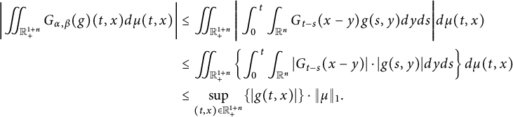 $$ \begin{align*} \left|\iint_{\mathbb R^{1+n}_{+}}G_{\alpha,\beta}(g)(t,x)d\mu(t,x)\right|&\leq \iint_{\mathbb R^{1+n}_{+}}\Bigg|\int^{t}_{0}\int_{\mathbb R^{n}}G_{t-s}(x-y)g(s,y)dyds\Bigg|d\mu(t,x)\\&\leq \iint_{\mathbb R^{1+n}_{+}}\left\{\int^{t}_{0}\int_{\mathbb R^{n}}|G_{t-s}(x-y)|\cdot|g(s,y)|dyds\right\}d\mu(t,x)\\&\leq \sup_{(t,x)\in \mathbb R^{1+n}_{+}}\{|g(t,x)|\}\cdot\|\mu\|_{1}. \end{align*} $$
Hence, an application of the Riesz representation theorem yields that there exists a Borel measure $\nu (\cdot ,\cdot )$
on
$\nu (\cdot ,\cdot )$
on $\mathbb R^{1+n}_{+}$
such that
$\mathbb R^{1+n}_{+}$
such that
 $$ \begin{align*} \iint_{\mathbb R^{1+n}_{+}}G_{\alpha,\beta}(g)(t,x)d\mu(t,x)=\iint_{\mathbb R^{1+n}_{+}}g(t,x)d\nu(t,x). \end{align*} $$
Proposition 3.1 For a compact subset $K\subset \mathbb R^{1+n}_{+}$
, let
$K\subset \mathbb R^{1+n}_{+}$
, let $\mathcal {M}_{+}(K)$
be the class of all positive measures on
$\mathcal {M}_{+}(K)$
be the class of all positive measures on $\mathbb R^{1+n}_{+}$
supported by K. If
$\mathbb R^{1+n}_{+}$
supported by K. If $1<p,q<\infty $
,
$1<p,q<\infty $
, $p'=p/(p-1)$
, and
$p'=p/(p-1)$
, and $q'=q/(q-1)$
, then
$q'=q/(q-1)$
, then
 $$ \begin{align*} C^{(\alpha,\beta)}_{p,q}(K)=\sup \left\{ \|\mu\|_{1}^{p\wedge q}:\, \mu\in \mathcal{M}_{+}(K)\ \&\ \|G^{\ast}_{\alpha,\beta}\mu\|_{L^{q'}_{t}L^{p'}_{x}(\mathbb R^{1+n}_{+})}\leq 1\right\}. \end{align*} $$
Proof Set
 $$ \begin{align*} \widetilde{C^{(\alpha,\beta)}_{p,q}}(K):=\sup\left\{\|\mu\|_{1}^{p\wedge q}:\, \mu\in \mathcal{M}_{+}(K)\ \&\ \|G^{\ast}_{\alpha,\beta}\mu\|_{L^{q'}_{t}L^{p'}_{x}(\mathbb R^{1+n}_{+})}\leq1\right\}. \end{align*} $$
For any $g\geq 0$
such that
$g\geq 0$
such that $\ G_{\alpha ,\beta }(g)\geq 1_{K}$
, by (3.1) and Hölder’s inequality, we have
$\ G_{\alpha ,\beta }(g)\geq 1_{K}$
, by (3.1) and Hölder’s inequality, we have
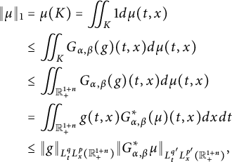 $$ \begin{align*} \|\mu\|_{1}&= \mu(K)=\iint_{K}1d\mu(t,x)\\ &\leq \iint_{K}G_{\alpha,\beta}(g)(t,x)d\mu(t,x)\\ &\leq \iint_{\mathbb R^{1+n}_{+}}G_{\alpha,\beta}(g)(t,x)d\mu(t,x)\\ &= \iint_{\mathbb R^{1+n}_{+}}g(t,x)G^{\ast}_{\alpha,\beta}(\mu)(t,x)dxdt\\ &\leq \|g\|_{L^{q}_{t}L^{p}_{x}(\mathbb R^{1+n}_{+})}\|G^{\ast}_{\alpha,\beta}\mu\|_{L^{q'}_{t}L^{p'}_{x}(\mathbb R^{1+n}_{+})}, \end{align*} $$
which implies that if $\mu $
satisfies
$\mu $
satisfies $\|G^{\ast }_{\alpha ,\beta }\mu \|_{L^{q'}_{t}L^{p'}_{x}(\mathbb R^{1+n}_{+})}\leq 1$
, then
$\|G^{\ast }_{\alpha ,\beta }\mu \|_{L^{q'}_{t}L^{p'}_{x}(\mathbb R^{1+n}_{+})}\leq 1$
, then $\|\mu \|_{1}^{p\wedge q}\leq \|g\|^{p\wedge q}_{L^{q}_{t}L^{p}_{x}(\mathbb R^{1+n}_{+})}$
, i.e.,
$\|\mu \|_{1}^{p\wedge q}\leq \|g\|^{p\wedge q}_{L^{q}_{t}L^{p}_{x}(\mathbb R^{1+n}_{+})}$
, i.e.,
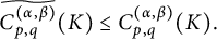 $$ \begin{align*} \widetilde{C^{(\alpha,\beta)}_{p,q}}(K)\leq C^{(\alpha,\beta)}_{p,q}(K). \end{align*} $$
Moreover, let
 $$ \begin{align*}\left\{\begin{aligned} &\mathcal X:=\Big\{\mu:\ \mu\in\mathcal M_{+}(K)\ \&\ \mu(K)=1\Big\},\\ &\mathcal Y:=\Big\{g:\ 0\leq g\in L^{q}_{t}L^{p}_{x}(\mathbb R^{1+n}_{+})\ \&\ \|g\|_{L^{q}_{t}L^{p}_{x}(\mathbb R^{1+n}_{+})}\leq 1\Big\},\\ &\mathcal Z:=\Big\{g:\ 0\leq g\in L^{q}_{t}L^{p}_{x}(\mathbb R^{1+n}_{+})\ \&\ G_{\alpha,\beta}(g)\geq 1_{K}\Big\}. \end{aligned}\right.\end{align*} $$
We have
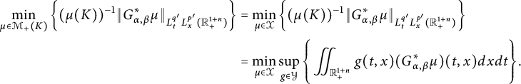 $$ \begin{align*} \min_{\mu\in\mathcal{M}_{+}(K)}\left\{(\mu(K))^{-1}\|G^{\ast}_{\alpha,\beta}\mu\|_{L^{q'}_{t}L^{p'}_{x}(\mathbb R^{1+n}_{+})}\right\} &= \min_{\mu\in\mathcal{X}} \left\{(\mu(K))^{-1}\|G^{\ast}_{\alpha,\beta} \mu\|_{L^{q'}_{t}L^{p'}_{x} (\mathbb R^{1+n}_{+})}\right\} \\ &= \min_{\mu\in\mathcal{X}}\sup_{g\in\mathcal{Y}}\Bigg\{\iint_{\mathbb R^{1+n}_{+}}g(t,x) (G^{\ast}_{\alpha,\beta}\mu)(t,x)dxdt\Bigg\}. \end{align*} $$
By [Reference Adams and Hedberg3, Theorem 2.4.1], we can deduce that
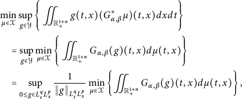 $$ \begin{align*} &\min_{\mu\in\mathcal{X}}\sup_{g\in\mathcal{Y}}\Bigg\{\iint_{\mathbb R^{1+n}_{+}}g(t,x)(G^{\ast}_{\alpha,\beta}\mu)(t,x)dxdt\Bigg\}\\ &\quad= \sup_{g\in\mathcal Y}\min_{\mu\in\mathcal{X}}\Bigg\{\iint_{\mathbb R^{1+n}_{+}} G_{\alpha,\beta}(g)(t,x)d\mu(t,x)\Bigg\}\\ &\quad= \sup_{0\leq g\in L^{q}_{t}L^{p}_{x}}\frac{1}{\|g\|_{L^{q}_{t}L^{p}_{x}}}\min_{\mu\in\mathcal{X}}\left\{\iint_{\mathbb R^{1+n}_{+}} G_{\alpha,\beta}(g)(t,x)d\mu(t,x)\right\}, \end{align*} $$
which implies
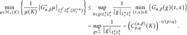 $$ \begin{align*} \min_{\mu\in\mathcal{M}_{+}(K)}\left\{\frac{1}{\mu(K)}\|G^{\ast}_{\alpha,\beta}\mu\|_{L^{q'}_{t}L^{p'}_{x}(\mathbb R^{1+n}_{+})}\right\} &\leq \sup_{0\leq g\in L^{q}_{t}L^{p}_{x}}\frac{1}{\|g\|_{L^{q}_{t}L^{p}_{x}}}\min_{(t,x)\in K}\left\{G_{\alpha,\beta}(g)(t,x)\right\}\\ &= \sup_{g\in\mathcal Z}\frac{1}{\|g\|_{L^{q}_{t}L^{p}_{x}}}=\left(C^{(\alpha,\beta)}_{p,q}(K)\right)^{-1/(p\wedge q)}. \end{align*} $$
Hence, it follows
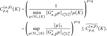 $$ \begin{align*} C^{(\alpha,\beta)}_{p,q}(K) &= \left(\frac{1}{\min\limits_{\mu\in\mathcal{M}_{+}(K)}{\|G^{\ast}_{\alpha,\beta} \mu\|_{L^{q}_{t}L^{p}_{x}}}/{\mu(K)}}\right)^{p\wedge q}\\ &=\left(\sup_{\mu\in\mathcal{M}_{+}(K)} \frac{\|\mu\|_{1}}{\|G^{\ast}_{\alpha,\beta}\mu \|_{L^{q}_{t}L^{p}_{x}}}\right)^{p\wedge q}\lesssim\widetilde{C^{(\alpha,\beta)}_{p,q}}(K).\\[-45pt] \end{align*} $$
3.2 Basic properties of the
$L^{q}_{t}L^p_{x}$
-capacity

Now, we are ready to establish the following basic properties of the $L^{q}_{t}L^p_{x}$
-capacities.
$L^{q}_{t}L^p_{x}$
-capacities.
Theorem 3.2 Assume that $\alpha>n$
and
$\alpha>n$
and $0<\beta <1$
. Let
$0<\beta <1$
. Let $1\leq p<\infty $
and
$1\leq p<\infty $
and $1<q<\infty $
.
$1<q<\infty $
.
-
(i)
$C^{(\alpha ,\beta )}_{p,q}(\emptyset )=0$
. Moreover, under
$K\subset \mathbb R^{1+n}_{+}$
and
$K\neq \emptyset $
,
$C^{(\alpha ,\beta )}_{p,q}(K)=0$
if and only if there exists
$0\leq g\in L^{q}_{t}L^{p}_{x}(\mathbb R^{1+n}_{+})$
such that
$$ \begin{align*} K\subseteq \Big\{(t,x)\in \mathbb R^{1+n}_{+}:\ G_{\alpha,\beta}(g)(t,x)=\infty\Big\}. \end{align*} $$
-
(ii) If
$E_{1}\subseteq E_{2}\subset \mathbb R^{1+n}_{+}$
,
$$ \begin{align*} C^{(\alpha,\beta)}_{p,q}(E_{1})\leq C^{(\alpha,\beta)}_{p,q}(E_{2}). \end{align*} $$
-
(iii) Let
$\{E_{j}\}^{\infty }_{j=1}$
be any sequence of subsets of
$\mathbb R^{1+n}_{+}$
,
$$ \begin{align*} C^{(\alpha,\beta)}_{p,q}\left(\bigcup^{\infty}_{j=1}E_{j}\right)\leq \sum^{\infty}_{j=1}C^{(\alpha,\beta)}_{p,q}(E_{j}). \end{align*} $$
-
(iv) For any
$K\subset \mathbb R^{1+n}_{+}$
and any
$x_{0}\in \mathbb R^{n}$
,
$$ \begin{align*} C^{(\alpha,\beta)}_{p,q}(K+(0, x_{0}))=C^{(\alpha,\beta)}_{p,q}(K). \end{align*} $$


Proof (i) If $K=\emptyset $
, then for
$K=\emptyset $
, then for $g(t,x)\equiv 0$
,
$g(t,x)\equiv 0$
, $1_{K}\equiv 0$
and
$1_{K}\equiv 0$
and $G_{\alpha ,\beta }(g)=1_{K}=0$
, which indicates that
$G_{\alpha ,\beta }(g)=1_{K}=0$
, which indicates that $C^{(\alpha ,\beta )}_{p,q}(\emptyset )=0$
. Set
$C^{(\alpha ,\beta )}_{p,q}(\emptyset )=0$
. Set
 $$ \begin{align*}K_{\lambda}=\Big\{(t,x)\in\mathbb R^{1+n}_{+}:\ g\geq 0\ \&\ G_{\alpha,\beta}(g)\geq \lambda\Big\}.\end{align*} $$
We can see that
 $$ \begin{align*} C^{(\alpha,\beta)}_{p,q}\kern-2pt\left(\kern-1pt\Big\{(t,x)\in\mathbb R^{1+n}_{+}:\ g\geq 0 \ \& \ G_{\alpha,\beta}(g)\geq \lambda\Big\}\kern-1pt\right) :=\inf\Big\{\|g\|_{L^{q}_{t}L^{p}_{x}}^{p\wedge q}:\ G\geq 0\ \& \ G_{\alpha,\beta}(G)\geq 1_{K_{\lambda}}\Big\}. \end{align*} $$
Take $g\geq 0$
and
$g\geq 0$
and $G_{\alpha ,\beta }(g)\geq \lambda $
on
$G_{\alpha ,\beta }(g)\geq \lambda $
on $K_{\lambda }$
such that the function
$K_{\lambda }$
such that the function $G=g/\lambda $
satisfies
$G=g/\lambda $
satisfies $G_{\alpha ,\beta }(G)\geq {(G_{\alpha ,\beta }(g))}/{\lambda }\geq 1_{K_{\lambda }},$
which means
$G_{\alpha ,\beta }(G)\geq {(G_{\alpha ,\beta }(g))}/{\lambda }\geq 1_{K_{\lambda }},$
which means
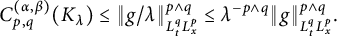 $$ \begin{align*}C^{(\alpha,\beta)}_{p,q}(K_{\lambda})\leq \|{g}/{\lambda}\|^{p\wedge q}_{L^{q}_{t}L^{p}_{x}}\leq \lambda^{-p\wedge q} \|g\|^{p\wedge q}_{L^{q}_{t}L^{p}_{x}}.\end{align*} $$
For any $(t,x)\in \mathcal {B}(G_{\alpha ,\beta }(g), p,q)$
,
$(t,x)\in \mathcal {B}(G_{\alpha ,\beta }(g), p,q)$
, $G_{\alpha ,\beta }(g)(t,x)=\infty $
. For any j,
$G_{\alpha ,\beta }(g)(t,x)=\infty $
. For any j, $G_{\alpha ,\beta }(g)(t,x)>2^{j}$
. Then
$G_{\alpha ,\beta }(g)(t,x)>2^{j}$
. Then
 $$ \begin{align*}(t,x)\in\Big\{(t,x)\in\mathbb R^{1+n}_{+}:\ g\geq 0\ \&\ G_{\alpha,\beta}(g)(t,x)>2^{j}\Big\},\end{align*} $$
that is,
 $$ \begin{align*}\mathcal{B}(G_{\alpha,\beta}(g), p,q)\subset \Big\{(t,x)\in\mathbb R^{1+n}_{+}:\ g\geq 0\ \&\ G_{\alpha,\beta}(g)(t,x)>2^{j}\Big\}.\end{align*} $$
We obtain
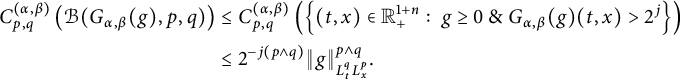 $$ \begin{align*} C^{(\alpha,\beta)}_{p,q}\left(\mathcal{B}(G_{\alpha,\beta}(g), p,q)\right)&\leq C^{(\alpha,\beta)}_{p,q}\left(\Big\{(t,x)\in\mathbb R^{1+n}_{+}:\ g\geq 0\ \&\ G_{\alpha,\beta}(g)(t,x)>2^{j}\Big\}\right)\\ &\leq 2^{-j(p\wedge q)}\|g\|^{p\wedge q}_{L^{q}_{t}L^{p}_{x}}. \end{align*} $$
Letting $j\rightarrow \infty $
gives
$j\rightarrow \infty $
gives $C^{(\alpha ,\beta )}_{p,q}(\mathcal {B}(G_{\alpha ,\beta }(g), p,q))=0.$
This shows that
$C^{(\alpha ,\beta )}_{p,q}(\mathcal {B}(G_{\alpha ,\beta }(g), p,q))=0.$
This shows that $C^{(\alpha ,\beta )}_{p,q}(K)=0$
if
$C^{(\alpha ,\beta )}_{p,q}(K)=0$
if $K\subseteq \mathcal {B}(G_{\alpha ,\beta }(g), p,q)$
.
$K\subseteq \mathcal {B}(G_{\alpha ,\beta }(g), p,q)$
.
Conversely, if $C^{(\alpha ,\beta )}_{p,q}(K)=0$
, from the definition of
$C^{(\alpha ,\beta )}_{p,q}(K)=0$
, from the definition of $C^{(\alpha ,\beta )}_{p,q}(\cdot )$
, we can see that
$C^{(\alpha ,\beta )}_{p,q}(\cdot )$
, we can see that
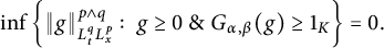 $$ \begin{align*} \inf\left\{\|g\|^{p\wedge q}_{L^{q}_{t}L^{p}_{x}}:\ g\geq 0\ \& \ G_{\alpha,\beta}(g)\geq 1_{K}\right\}=0. \end{align*} $$
Then, for any $j\in \mathbb Z$
, there exists
$j\in \mathbb Z$
, there exists $g_{j}$
such that
$g_{j}$
such that $g_{j}\geq 0$
and
$g_{j}\geq 0$
and $G_{\alpha ,\beta }(g_{j})\geq 1$
on K satisfying
$G_{\alpha ,\beta }(g_{j})\geq 1$
on K satisfying $\|g_{j}\|^{p\wedge q}_{L^{q}_{t}L^{p}_{x}}<2^{-j}$
. Let
$\|g_{j}\|^{p\wedge q}_{L^{q}_{t}L^{p}_{x}}<2^{-j}$
. Let $g=\sum ^{\infty }_{j=1}g_{j}$
. It is obvious that
$g=\sum ^{\infty }_{j=1}g_{j}$
. It is obvious that $g\geq 0$
and
$g\geq 0$
and $G_{\alpha ,\beta }(g)=\infty $
on K, which implies that
$G_{\alpha ,\beta }(g)=\infty $
on K, which implies that $K\subset \mathcal {B}(G_{\alpha ,\beta }, g, p,q)$
.
$K\subset \mathcal {B}(G_{\alpha ,\beta }, g, p,q)$
.
(ii) Let $K_{1}\subseteq K_{2}$
. Then
$K_{1}\subseteq K_{2}$
. Then $1_{K_{1}}(t,x)\leq 1_{K_{2}}(t,x)$
and
$1_{K_{1}}(t,x)\leq 1_{K_{2}}(t,x)$
and
 $$ \begin{align} \qquad\ \Big\{\|g\|^{p\wedge q}_{L^{q}_{t}L^{p}_{x}}:\ g\geq 0\ \& \ G_{\alpha,\beta}(g)\geq 1_{K_{2}}\Big\}\subseteq \Big\{\|g\|^{p\wedge q}_{L^{q}_{t}L^{p}_{x}}:\ g\geq 0\ \& \ G_{\alpha,\beta}(g)\geq 1_{K_{1}}\Big\}.\!\!\!\!\!\!\!\!\!\!\!\! \end{align} $$
Taking the infimum on both sides of (3.2) yields $C^{(\alpha ,\beta )}_{p,q}(K_{1})\leq C^{(\alpha ,\beta )}_{p,q}(K_{2}).$
(iii) The proof of this assertion is divided into two cases.
Case 1: $p\ge q$
, i.e.,
$p\ge q$
, i.e., $q=p\wedge q$
. Let
$q=p\wedge q$
. Let $\{g_{j}\}$
be a sequence of functions such that
$\{g_{j}\}$
be a sequence of functions such that $G_{\alpha ,\beta }(g_{j})\geq 1$
on
$G_{\alpha ,\beta }(g_{j})\geq 1$
on $E_{j}$
. Define
$E_{j}$
. Define $g:=\sup _{j}g_{j}$
which satisfies
$g:=\sup _{j}g_{j}$
which satisfies $G_{\alpha ,\beta }(g)\geq 1$
on
$G_{\alpha ,\beta }(g)\geq 1$
on $\bigcup ^{\infty }_{j=1}E_{j}$
. We can get
$\bigcup ^{\infty }_{j=1}E_{j}$
. We can get
 $$ \begin{align*} \|g\|^{q}_{L^{q}_{t}L^{p}_{x}(\mathbb R^{1+n}_{+})} = \Bigg\{\kern-1.5pt\!\int^{\infty}_{0}\Bigg(\kern-1.5pt\!\int_{\mathbb R^{n}}|g(t,x)|^{p}dx\kern-1pt\Bigg)^{q/p}dt\Bigg\} \leq\sum^{\infty}_{j=1}\Bigg\{\!\kern-1.5pt\int^{\infty}_{0}\!\Bigg(\!\int_{\mathbb R^{n}}|g_{j}(t,x)|^{p}dx\kern-1.5pt\Bigg)^{q/p}dt\Bigg\}. \end{align*} $$
This implies that
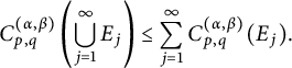 $$ \begin{align*} C^{(\alpha,\beta)}_{p,q}\left(\bigcup^{\infty}_{j=1}E_{j}\right)\leq \sum^{\infty}_{j=1}C^{(\alpha,\beta)}_{p,q}(E_{j}). \end{align*} $$
Case 2: $p<q$
, i.e.,
$p<q$
, i.e., $p\wedge q=p$
. For
$p\wedge q=p$
. For $\{g_{j}\}$
such that
$\{g_{j}\}$
such that $g_{j}\geq 0$
and
$g_{j}\geq 0$
and $G_{\alpha ,\beta }(g_{j})\geq 1$
on
$G_{\alpha ,\beta }(g_{j})\geq 1$
on $E_{j}$
, let
$E_{j}$
, let $g=\sup _{j}g_{j}$
. For
$g=\sup _{j}g_{j}$
. For $(t,x)\in \bigcup ^{\infty }_{j=1}E_{j}$
, there exists a
$(t,x)\in \bigcup ^{\infty }_{j=1}E_{j}$
, there exists a $j_{0}$
such that
$j_{0}$
such that $(t,x)\in E_{j_{0}}$
. Then
$(t,x)\in E_{j_{0}}$
. Then $g(t,x)\geq g_{j_{0}}(t,x)\geq 0$
, i.e.,
$g(t,x)\geq g_{j_{0}}(t,x)\geq 0$
, i.e., $g\ge 0$
on
$g\ge 0$
on $\bigcup ^{\infty }_{j=1}E_{j}$
. We get
$\bigcup ^{\infty }_{j=1}E_{j}$
. We get $G_{\alpha ,\beta }(g)(t,x)\geq G_{\alpha ,\beta }(g_{j_{0}})(t,x)\geq 0$
for
$G_{\alpha ,\beta }(g)(t,x)\geq G_{\alpha ,\beta }(g_{j_{0}})(t,x)\geq 0$
for $ (t,x)\in \bigcup ^{\infty }_{j=1}E_{j}.$
This indicates that
$ (t,x)\in \bigcup ^{\infty }_{j=1}E_{j}.$
This indicates that
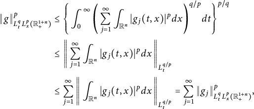 $$ \begin{align*} \|g\|^{p}_{L^{q}_{t}L^{p}_{x}(\mathbb R^{1+n}_{+})} &\leq \Bigg\{\int^{\infty}_{0}\Bigg(\sum^{\infty}_{j=1}\int_{\mathbb R^{n}}|g_{j}(t,x)|^{p}dx\Bigg)^{q/p}dt\Bigg\}^{p/q}\\ &\leq \Bigg\|\sum^{\infty}_{j=1}\int_{\mathbb R^{n}}|g_{j}(t,x)|^{p}dx\Bigg\|_{L^{q/p}_{t}}\\ &\leq \sum^{\infty}_{j=1}\Bigg\|\int_{\mathbb R^{n}}|g_{j}(t,x)|^{p}dx\Bigg\|_{L^{q/p}_{t}} =\sum^{\infty}_{j=1}\|g_{j}\|^{p}_{L^{q}_{t}L^{p}_{x}(\mathbb R^{1+n}_{+})}, \end{align*} $$
which gives
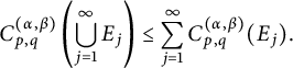 $$ \begin{align*} C^{(\alpha,\beta)}_{p,q}\left(\bigcup^{\infty}_{j=1}E_{j}\right)\leq \sum^{\infty}_{j=1}C^{(\alpha,\beta)}_{p,q}(E_{j}). \end{align*} $$
(iv) Because $g_{x_{0}}(x,t)=g(t, x+x_{0})$
, it is easy to see that
$g_{x_{0}}(x,t)=g(t, x+x_{0})$
, it is easy to see that $\|g_{x_{0}}\|_{L^{q}_{t}L^{p}_{x}}=\|g\|_{L^{q}_{t}L^{p}_{x}}$
and
$\|g_{x_{0}}\|_{L^{q}_{t}L^{p}_{x}}=\|g\|_{L^{q}_{t}L^{p}_{x}}$
and
 $$ \begin{align*}C^{(\alpha,\beta)}_{p,q}(K+(0, x_{0}))=C^{(\alpha,\beta)}_{p,q}(K).\\[-36pt]\end{align*} $$
At the end of this subsection, we investigate the inner and outer capacitary properties of $C^{(\alpha ,\beta )}_{p,q}(\cdot )$
. We first prove that the capacity
$C^{(\alpha ,\beta )}_{p,q}(\cdot )$
. We first prove that the capacity $C^{(\alpha ,\beta )}_{p,q}(\cdot )$
is an outer capacity.
$C^{(\alpha ,\beta )}_{p,q}(\cdot )$
is an outer capacity.
Proposition 3.3 For any $E\subset \mathbb R^{n+1}_{+}$
,
$E\subset \mathbb R^{n+1}_{+}$
,
 $$ \begin{align*}C^{(\alpha,\beta)}_{p,q}(E)=\inf\Big\{C^{(\alpha,\beta)}_{p,q}(O):\ O\supset E\ \& \ O\text{ open}\Big\}.\end{align*} $$
Proof Without loss of generality, we assume that $C^{(\alpha ,\beta )}_{p,q}(E)<\infty $
. By (ii) of Theorem 3.2,
$C^{(\alpha ,\beta )}_{p,q}(E)<\infty $
. By (ii) of Theorem 3.2,
 $$ \begin{align*}C^{(\alpha,\beta)}_{p,q}(E)\leq\inf\Big\{C^{(\alpha,\beta)}_{p,q}(O):\ O\supset E \ \& \ O\text{ open}\Big\}.\end{align*} $$
For $\epsilon \in (0,1)$
, there exists a measurable, nonnegative function f such that
$\epsilon \in (0,1)$
, there exists a measurable, nonnegative function f such that $G_{\alpha ,\beta }f\geq 1$
on E and
$G_{\alpha ,\beta }f\geq 1$
on E and $\|f\|_{L^{q}_{t}L^{p}_{x}}^{p\wedge q}\leq C^{(\alpha ,\beta )}_{p,q}(E)+\epsilon .$
Since
$\|f\|_{L^{q}_{t}L^{p}_{x}}^{p\wedge q}\leq C^{(\alpha ,\beta )}_{p,q}(E)+\epsilon .$
Since $G_{\alpha ,\beta }f$
is lower semicontinuous, then the set
$G_{\alpha ,\beta }f$
is lower semicontinuous, then the set $O_{\epsilon }:=\{(x,t)\in \mathbb R^{n+1}_{+}:\ G_{\alpha ,\beta }f(x,t)>1-\epsilon \}$
is an open set. On the other hand,
$O_{\epsilon }:=\{(x,t)\in \mathbb R^{n+1}_{+}:\ G_{\alpha ,\beta }f(x,t)>1-\epsilon \}$
is an open set. On the other hand, $E\subset O_{\epsilon }$
. This implies that
$E\subset O_{\epsilon }$
. This implies that
 $$ \begin{align*}C^{(\alpha,\beta)}_{p,q}(O_{\epsilon})&\leq \frac{1}{(1-\epsilon)^{p\wedge q}}\left(\int^{\infty}_{0}\left(\int_{\mathbb R^{n}}|f(x)|^{p}dx\right)^{q/p}dt\right)^{(p\wedge q)/q}\\&<\frac{1}{(1-\epsilon)^{p\wedge q}}(C^{(\alpha,\beta)}_{p,q}(E)+\epsilon).\end{align*} $$
The arbitrariness of $\epsilon $
indicates that
$\epsilon $
indicates that
 $$ \begin{align*}C^{(\alpha,\beta)}_{p,q}(E)\geq\inf\Big\{C^{(\alpha,\beta)}_{p,q}(O):\ O\supset E \ \& \ O\text{ open}\Big\}.\\[-37pt]\end{align*} $$
The following result can be deduced from Proposition 2.1 as an immediate corollary.
Corollary 3.4 If $K_{j}$
is a decreasing sequence of compact sets, then
$K_{j}$
is a decreasing sequence of compact sets, then
 $$ \begin{align*}C^{(\alpha,\beta)}_{p,q}(\cap^{\infty}_{j=1}K_{j})=\lim_{j\rightarrow\infty} C^{(\alpha,\beta)}_{p,q}(K_{j}).\end{align*} $$
Proposition 3.5 Let $1<p<\infty $
and
$1<p<\infty $
and $1<q<\infty $
. If
$1<q<\infty $
. If $\{E_{j}\}^{\infty }_{j=1}$
is an increasing sequence of arbitrary subsets of
$\{E_{j}\}^{\infty }_{j=1}$
is an increasing sequence of arbitrary subsets of $\mathbb R^{n}$
, then
$\mathbb R^{n}$
, then
 $$ \begin{align*}C^{(\alpha,\beta)}_{p,q}(\cup^{\infty}_{j=1}E_{j})=\lim_{j\rightarrow\infty}C^{(\alpha,\beta)}_{p,q}(E_{j}).\end{align*} $$
Proof Since $\{E_{j}\}^{\infty }_{j=1}$
is increasing, then
$\{E_{j}\}^{\infty }_{j=1}$
is increasing, then
 $$ \begin{align*}C^{(\alpha,\beta)}_{p,q}(\cup^{\infty}_{j=1}E_{j})\geq\lim_{j\rightarrow\infty}C^{(\alpha,\beta)}_{p,q}(E_{j}).\end{align*} $$
Conversely, without loss of generality, we assume that $\lim \limits _{j\rightarrow \infty }C^{(\alpha ,\beta )}_{p,q}(E_{j})$
is finite. For each j, let
$\lim \limits _{j\rightarrow \infty }C^{(\alpha ,\beta )}_{p,q}(E_{j})$
is finite. For each j, let $f_{E_{j}}$
be the unique function such that
$f_{E_{j}}$
be the unique function such that $f_{E_{j}}\geq 1$
on
$f_{E_{j}}\geq 1$
on $E_{j}$
and
$E_{j}$
and $\|f_{E_{j}}\|^{p\wedge q}_{L^{q}_{t}L^{p}_{x}}=C^{(\alpha ,\beta )}_{p,q}(E_{j})$
. Then, for
$\|f_{E_{j}}\|^{p\wedge q}_{L^{q}_{t}L^{p}_{x}}=C^{(\alpha ,\beta )}_{p,q}(E_{j})$
. Then, for $i<j$
, it holds that
$i<j$
, it holds that $G_{\alpha ,\beta }f_{E_{j}}\geq 1$
on
$G_{\alpha ,\beta }f_{E_{j}}\geq 1$
on $E_{i}$
and further,
$E_{i}$
and further, $G_{\alpha ,\beta }((f_{E_{i}}+f_{E_{j}})/2)\geq 1$
on
$G_{\alpha ,\beta }((f_{E_{i}}+f_{E_{j}})/2)\geq 1$
on $E_{i}$
, which means that
$E_{i}$
, which means that
 $$ \begin{align*} \left(\int^{\infty}_{0}\left(\int_{\mathbb R^{n}}((f_{E_{i}}+f_{E_{j}})(x,t)/2)^{p}dx\right)^{q/p}dt\right)^{(p \wedge q)/q}\geq C^{(\alpha,\beta)}_{p,q}(E_{i}). \end{align*} $$
Since the space $L^{q}_{t}L^{p}_{x}(\mathbb R^{n+1}_{+})$
is a uniformly convex Banach space for
$L^{q}_{t}L^{p}_{x}(\mathbb R^{n+1}_{+})$
is a uniformly convex Banach space for $1<p<\infty $
and
$1<p<\infty $
and $1<q<\infty $
(cf. [Reference Benedek and Panzone7, Theorem 1, p. 317]), by [Reference Adams and Hedberg3, Corollary 1.3.3], the sequence
$1<q<\infty $
(cf. [Reference Benedek and Panzone7, Theorem 1, p. 317]), by [Reference Adams and Hedberg3, Corollary 1.3.3], the sequence $\{f_{E_{j}}\}^{\infty }_{j=1}$
converges strongly to a function f satisfying
$\{f_{E_{j}}\}^{\infty }_{j=1}$
converges strongly to a function f satisfying
 $$ \begin{align*} \|f\|^{p\wedge q}_{L^{q}_{t}L^{p}_{x}}=\lim_{j\rightarrow\infty}C^{(\alpha,\beta)}_{p,q}(E_{j}). \end{align*} $$
Similar to [Reference Adams and Hedberg3, Proposition 2.3.12], we can prove that $G_{\alpha ,\beta }f\geq 1$
on
$G_{\alpha ,\beta }f\geq 1$
on $\cup ^{\infty }_{j=1}E_{j}$
, except possibly on a countable union of sets with
$\cup ^{\infty }_{j=1}E_{j}$
, except possibly on a countable union of sets with $C^{(\alpha ,\beta )}_{p,q}(\cdot )$
zero. Hence,
$C^{(\alpha ,\beta )}_{p,q}(\cdot )$
zero. Hence,
 $$ \begin{align*} \lim_{j\rightarrow\infty}C^{(\alpha,\beta)}_{p,q}(E_{j})\geq\|f\|^{p\wedge q}_{L^{q}_{t}L^{p}_{x}}\geq C^{(\alpha,\beta)}_{p,q}(\cup^{\infty}_{j=1}E_{j}).\\[-40pt] \end{align*} $$
As a corollary of Proposition 3.5, we can get the following result.
Corollary 3.6 Assume that $1<p<\infty $
and
$1<p<\infty $
and $1<q<\infty $
. Let O be an open subset of
$1<q<\infty $
. Let O be an open subset of $\mathbb R^{n+1}_{+}$
. Then
$\mathbb R^{n+1}_{+}$
. Then
 $$ \begin{align*} C^{(\alpha,\beta)}_{p,q}(O)=\sup\left\{C^{(\alpha,\beta)}_{p,q}(K):\ \text{ compact }K\subset O\right\}.\end{align*} $$
3.3
$L^{q}_{t}L^p_{x}$
-capacity of fractional parabolic balls in
$\mathbb R^{1+n}_{+}$


For $(t_{0}, x_{0}, r)\in (0,\infty )\times \mathbb R^{n}\times (0,\infty )$
, the fractional parabolic ball is defined as
$(t_{0}, x_{0}, r)\in (0,\infty )\times \mathbb R^{n}\times (0,\infty )$
, the fractional parabolic ball is defined as
 $$ \begin{align*} B^{(\alpha,\beta)}_{r}(t_{0}, x_{0})=\Big\{(t,x)\in\mathbb R^{1+n}_{+},\ r^{\alpha}<t-t_{0}<2r^{\alpha}, |x-x_{0}|<r^{\beta}/2\Big\}. \end{align*} $$
Theorem 3.7 Assume that $(\alpha ,\beta ,p,q)\in (n,\infty )\times (0,1)\times [1,\infty )\times (1,\infty )$
satisfying
$(\alpha ,\beta ,p,q)\in (n,\infty )\times (0,1)\times [1,\infty )\times (1,\infty )$
satisfying $n\beta /p+\alpha /q-\alpha>0$
. Then, as
$n\beta /p+\alpha /q-\alpha>0$
. Then, as $r_{0}\rightarrow 0$
and
$r_{0}\rightarrow 0$
and $(t_{0},x_{0})\in \mathbb R^{1+n}_{+}$
,
$(t_{0},x_{0})\in \mathbb R^{1+n}_{+}$
,
 $$ \begin{align*} C^{(\alpha,\beta)}_{p,q}(B^{(\alpha,\beta)}_{r_{0}}(t_{0},x_{0}))\simeq r_{0}^{(p\wedge q)(n\beta/p+\alpha/q-\alpha)}. \end{align*} $$
Proof We first assume that $(t_{0},x_{0})=(0,0)$
. Let
$(t_{0},x_{0})=(0,0)$
. Let $g\geq 0$
satisfying
$g\geq 0$
satisfying $G_{\alpha ,\beta }(g)(t,x)\geq 1_{B_{r_{0}}^{(\alpha ,\beta )}(0,0)}(t,x)$
. If
$G_{\alpha ,\beta }(g)(t,x)\geq 1_{B_{r_{0}}^{(\alpha ,\beta )}(0,0)}(t,x)$
. If $(t,x)\in B_{r_{0}}^{(\alpha ,\beta )}(0,0)$
, then
$(t,x)\in B_{r_{0}}^{(\alpha ,\beta )}(0,0)$
, then $|t|<2r_{0}^{\alpha }$
and
$|t|<2r_{0}^{\alpha }$
and $|x|<r^{\beta }_{0}/2$
. We can see that
$|x|<r^{\beta }_{0}/2$
. We can see that $(t,x)\in B_{r_{0}}^{(\alpha ,\beta )}(0,0)$
if and only if
$(t,x)\in B_{r_{0}}^{(\alpha ,\beta )}(0,0)$
if and only if $(s,y)\in B_{1}^{(\alpha ,\beta )}(0,0)$
, where
$(s,y)\in B_{1}^{(\alpha ,\beta )}(0,0)$
, where $s=t/r^{\alpha }_{0}$
and
$s=t/r^{\alpha }_{0}$
and $y=x/r_{0}^{\beta }$
. Then, by (2.5), we utilize the change of variables
$y=x/r_{0}^{\beta }$
. Then, by (2.5), we utilize the change of variables $r^{-\alpha }_{0}u=v\ \&\ r^{-\beta }_{0}z=w$
to deduce that
$r^{-\alpha }_{0}u=v\ \&\ r^{-\beta }_{0}z=w$
to deduce that
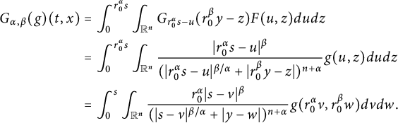 $$ \begin{align*} G_{\alpha,\beta}(g)(t,x) &= \int^{r^{\alpha}_{0}s}_{0}\int_{\mathbb R^{n}}G_{r^{\alpha}_{0}s-u}(r^{\beta}_{0}y-z)F(u,z)dudz\\ &= \int^{r^{\alpha}_{0}s}_{0}\int_{\mathbb R^{n}}\frac{|r^{\alpha}_{0}s-u|^{\beta}}{(|r^{\alpha}_{0}s-u|^{\beta/\alpha}+|r^{\beta}_{0}y-z|)^{n+\alpha}}g(u,z)dudz\\ &= \int^{s}_{0}\int_{\mathbb R^{n}}\frac{r^{\alpha}_{0}|s-v|^{\beta}}{(|s-v|^{\beta/\alpha}+|y-w|)^{n+\alpha}} g(r^{\alpha}_{0}v, r^{\beta}_{0}w)dvdw. \end{align*} $$
Denote $r^{\alpha }_{0}g(r^{\alpha }_{0}t, r^{\beta }_{0}x)$
by
$r^{\alpha }_{0}g(r^{\alpha }_{0}t, r^{\beta }_{0}x)$
by $g^{\ast }(t,x)$
. The above computation gives
$g^{\ast }(t,x)$
. The above computation gives
 $$ \begin{align*}G_{\alpha,\beta}(g)(t,x)=G_{\alpha,\beta}(g^{\ast})(s,y).\end{align*} $$
This means that $G_{\alpha ,\beta }(g)(t,x)\geq 1$
for
$G_{\alpha ,\beta }(g)(t,x)\geq 1$
for $(t,x)\in B_{r_{0}}^{(\alpha ,\beta )}(0,0)$
if and only if
$(t,x)\in B_{r_{0}}^{(\alpha ,\beta )}(0,0)$
if and only if $G_{\alpha ,\beta }(g^{\ast })(s,y)\geq 1$
for
$G_{\alpha ,\beta }(g^{\ast })(s,y)\geq 1$
for $(s,y)\in B_{1}^{(\alpha ,\beta )}(0,0)$
. It is easy to get
$(s,y)\in B_{1}^{(\alpha ,\beta )}(0,0)$
. It is easy to get
 $$ \begin{align*}C^{(\alpha,\beta)}_{p,q}(B_{1}^{(\alpha,\beta)}(0,0))\leq \|g^{\ast}\|_{L^{q}_{t}L^{p}_{x}(\mathbb R^{1+n}_{+})}^{p\wedge q} =\|r^{\alpha}_{0}g(r^{\alpha}_{0}\cdot, r^{\beta}_{0}\cdot)\|_{L^{q}_{t}L^{p}_{x}(\mathbb R^{1+n}_{+})}^{p\wedge q}.\end{align*} $$
Below a change of variables gives
 $$ \begin{align*} \|r^{\alpha}_{0}g(r^{\alpha}_{0}\cdot, r^{\beta}_{0}\cdot)\|_{L^{q}_{t}L^{p}_{x}(\mathbb R^{1+n}_{+})}^{p\wedge q} &=\Bigg\{\int^{\infty}_{0}\Bigg(\int_{\mathbb R^{n}}|r^{\alpha}_{0}g(r^{\alpha}_{0}t, r^{\beta}_{0}x)|^{p}dx\Bigg)^{q/p}dt\Bigg\}^{(p\wedge q)/q} \\&= r^{(\alpha-\beta n/p-\alpha/q)(p\wedge q)}\|g\|_{L^{q}_{t}L^{p}_{x}(\mathbb R^{1+n}_{+})}^{p\wedge q}, \end{align*} $$
which indicates that
 $$ \begin{align*}C^{(\alpha,\beta)}_{p,q}(B_{1}^{(\alpha,\beta)}(0,0))\leq \|g^{\ast}\|_{L^{q}_{t}L^{p}_{x}(\mathbb R^{1+n}_{+})}^{p\wedge q}\leq r^{(\alpha-\beta n/p-\alpha/q)(p\wedge q)}\|g\|_{L^{q}_{t}L^{p}_{x}(\mathbb R^{1+n}_{+})}^{p\wedge q}.\end{align*} $$
By the arbitrariness of g, we know
 $$ \begin{align*} C^{(\alpha,\beta)}_{p,q}(B_{1}^{(\alpha,\beta)}(0,0))\leq r^{(\alpha-\beta n/p-\alpha/q)(p\wedge q)}C^{(\alpha,\beta)}_{p,q}(B_{r_{0}}^{(\alpha,\beta)}(0,0)). \end{align*} $$
Changing the order of $B_{r_{0}}^{(\alpha ,\beta )}(0,0)$
and
$B_{r_{0}}^{(\alpha ,\beta )}(0,0)$
and $B_{1}^{(\alpha ,\beta )}(0,0)$
, similarly, it holds
$B_{1}^{(\alpha ,\beta )}(0,0)$
, similarly, it holds
 $$ \begin{align*} C^{(\alpha,\beta)}_{p,q}(B_{r_{0}}^{(\alpha,\beta)}(0,0))\leq r^{-(\alpha-\beta n/p-\alpha/q)(p\wedge q)}C^{(\alpha,\beta)}_{p,q}(B_{1}^{(\alpha,\beta)}(0,0)). \end{align*} $$
This shows that
 $$ \begin{align*} C^{(\alpha,\beta)}_{p,q}(B_{r_{0}}^{(\alpha,\beta)}(0,0))\simeq r_{0}^{(p\wedge q)(n\beta/p+\alpha/q-\alpha)}. \end{align*} $$
Now, for arbitrary $(t_{0},x_{0})\in \mathbb R^{1+n}_{+}$
, let
$(t_{0},x_{0})\in \mathbb R^{1+n}_{+}$
, let $g\geq 0$
and
$g\geq 0$
and $G_{\alpha ,\beta }(g)\geq 1_{B^{(\alpha ,\beta )}_{r_{0}}(t_{0},x_{0})}$
. Then, for
$G_{\alpha ,\beta }(g)\geq 1_{B^{(\alpha ,\beta )}_{r_{0}}(t_{0},x_{0})}$
. Then, for $1\leq p<\infty $
and
$1\leq p<\infty $
and $1<q<\infty $
, there exist
$1<q<\infty $
, there exist $\widetilde {p}$
and
$\widetilde {p}$
and $\widetilde {q}$
such that
$\widetilde {q}$
such that
 $$ \begin{align*}\begin{cases} 1\leq p<\widetilde{p}<\infty,\\ 1<q<\widetilde{q}<\infty,\\ (1/q-1/\widetilde{q})+({\beta n}/{\alpha})(1/p-1/\widetilde{p})=1. \end{cases}\end{align*} $$
By Theorem 2.6, $\|G_{\alpha ,\beta }(g)\|_{L^{\widetilde {q}}_{t}L^{\widetilde {p}}_{x}(\mathbb R^{1+n}_{+})}\lesssim \|g\|_{L^{q}_{t}L^{p}_{x}(\mathbb R^{1+n}_{+})}.$
It is obvious that
$\|G_{\alpha ,\beta }(g)\|_{L^{\widetilde {q}}_{t}L^{\widetilde {p}}_{x}(\mathbb R^{1+n}_{+})}\lesssim \|g\|_{L^{q}_{t}L^{p}_{x}(\mathbb R^{1+n}_{+})}.$
It is obvious that
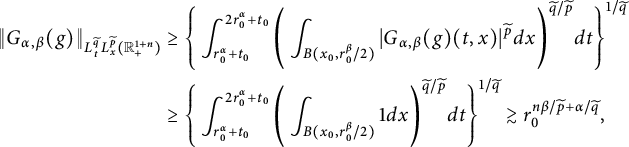 $$ \begin{align*} \|G_{\alpha,\beta}(g)\|_{L^{\widetilde{q}}_{t}L^{\widetilde{p}}_{x}(\mathbb R^{1+n}_{+})} &\geq \Bigg\{\int^{2r^{\alpha}_{0}+t_{0}}_{r_{0}^{\alpha}+t_{0}}\Bigg(\int_{B(x_{0}, r^{\beta}_{0}/2)}|G_{\alpha,\beta}(g)(t,x)|^{\widetilde{p}}dx\Bigg)^{\widetilde{q}/\widetilde{p}}dt\Bigg\}^{1/\widetilde{q}}\\ &\geq \Bigg\{\int^{2r^{\alpha}_{0}+t_{0}}_{r_{0}^{\alpha}+t_{0}}\Bigg(\int_{B(x_{0}, r^{\beta}_{0}/2)}1dx\Bigg)^{\widetilde{q}/\widetilde{p}}dt\Bigg\}^{1/\widetilde{q}} \gtrsim r_{0}^{n\beta/\widetilde{p}+\alpha/\widetilde{q}}, \end{align*} $$
which implies $r_{0}^{(n\beta /\widetilde {p}+\alpha /\widetilde {q})(p\wedge q)}\lesssim \|g\|^{p\wedge q}_{L^{q}_{t}L^{p}_{x}(\mathbb R^{1+n}_{+})}.$
Since
$r_{0}^{(n\beta /\widetilde {p}+\alpha /\widetilde {q})(p\wedge q)}\lesssim \|g\|^{p\wedge q}_{L^{q}_{t}L^{p}_{x}(\mathbb R^{1+n}_{+})}.$
Since $(1/q-1/\widetilde {q})+(\beta n/\alpha )(1/p-1/\widetilde {p})=1$
, the arbitrariness of g shows that
$(1/q-1/\widetilde {q})+(\beta n/\alpha )(1/p-1/\widetilde {p})=1$
, the arbitrariness of g shows that
 $$ \begin{align*} r_{0}^{(\alpha/q+n\beta/p-\alpha)(p\wedge q)}\lesssim C^{(\alpha,\beta)}_{p,q}(B^{(\alpha,\beta)}_{r_{0}}(t_{0},x_{0})). \end{align*} $$
Below, we investigate the upper bound of $C^{(\alpha ,\beta )}_{p,q}(B^{(\alpha ,\beta )}_{r_{0}}(t_{0},x_{0}))$
. Consider the ball
$C^{(\alpha ,\beta )}_{p,q}(B^{(\alpha ,\beta )}_{r_{0}}(t_{0},x_{0}))$
. Consider the ball
 $$ \begin{align*} B^{(\alpha,\beta)}_{r_{0},\eta}(t_{0},x_{0})=\left\{(t,x)\in\mathbb R^{1+n}_{+}:\ |t-t_{0}|<(\eta r_{0})^{\alpha}\ \& \ |x-x_{0}|<r^{\beta}_{0}\right\}, \end{align*} $$
where $\eta $
is a sufficiently large constant. Since
$\eta $
is a sufficiently large constant. Since $(t,x)\in B^{(\alpha ,\beta )}_{r_{0},\eta }(t_{0},x_{0})$
ensures that we have, for
$(t,x)\in B^{(\alpha ,\beta )}_{r_{0},\eta }(t_{0},x_{0})$
ensures that we have, for $r_{0}> 0$
small enough,
$r_{0}> 0$
small enough,
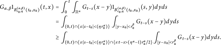 $$ \begin{align*} G_{\alpha,\beta}1_{B^{(\alpha,\beta)}_{r_{0},\eta}(t_{0},x_{0})}(t,x)&= \int^{t}_{0}\int_{\mathbb R^{n}}G_{t-s}(x-y)1_{B^{(\alpha,\beta)}_{r_{0},\eta}(t_{0},x_{0})}(s,y)dyds\\ &= \int_{(0,t)\cap\{s: |s-t_{0}|<(\eta r_{0}^{\alpha})\}}\int_{|y-x_{0}|<r^{\beta}_{0}}G_{t-s}(x-y)dyds\\ &\geq \int_{(0,t)\cap\{s: |s-t_{0}|<(\eta r_{0}^{\alpha})\}\cap \{s: t-s>(\eta^{\alpha}-1)r_{0}^{\alpha}/2\}}\!\int_{|y-x_{0}|<r^{\beta}_{0}}G_{t-s}(x\kern1.3pt{-}\kern1.3pt y)dyds. \end{align*} $$
Because $t-s>(\frac {\eta ^{\alpha }-1}{2})r_{0}^{\alpha }$
and
$t-s>(\frac {\eta ^{\alpha }-1}{2})r_{0}^{\alpha }$
and $|y-x_{0}|<r^{\beta }_{0}$
, then
$|y-x_{0}|<r^{\beta }_{0}$
, then $|y-x_{0}|< (\frac {\eta ^{\alpha }-1}{2})^{-\beta /\alpha }(t-s)^{\beta /\alpha }$
and
$|y-x_{0}|< (\frac {\eta ^{\alpha }-1}{2})^{-\beta /\alpha }(t-s)^{\beta /\alpha }$
and
 $$ \begin{align*} G_{t-s}(x-y)\gtrsim\frac{(t-s)^{\beta}}{(|x-y|+|t-s|^{\beta/\alpha})^{n+\alpha}} \gtrsim(\frac{\eta^{\alpha}-1}{2})^{\beta(n/\alpha+1)} (t-s)^{-n\beta/\alpha}. \end{align*} $$
If $|t-t_{0}|<r^{\alpha }_{0}$
,
$|t-t_{0}|<r^{\alpha }_{0}$
,
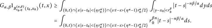 $$ \begin{align*} G_{\alpha,\beta}1_{B^{(\alpha,\beta)}_{r_{0},\eta}(t_{0},x_{0})}(t,x)&\geq \int_{(0,t)\cap\{s: |s-t_{0}|<(\eta r_{0}^{\alpha})\}\cap \{s: t-s>(\eta^{\alpha}-1)r_{0}^{\alpha}/2\}}\int_{|y-x_{0}|<r^{\beta}_{0}}|t-s|^{-n\beta/\alpha}dyds\\ &= \int_{(0,t)\cap\{s: |s-t_{0}|<(\eta r_{0}^{\alpha})\}\cap \{s: t-s>(\eta^{\alpha}-1)r_{0}^{\alpha}/2\}}r_{0}^{\beta n}|t-s|^{-n\beta/\alpha}ds. \end{align*} $$
It is easy to see that if $\eta>> 1$
and
$\eta>> 1$
and
 $$ \begin{align*}\begin{cases} 0<s<t,\\ t_{0}-(\eta r_{0})^{\alpha}<s<t_{0}+(\eta r_{0})^{\alpha},\\ s>t+\frac{\eta^{\alpha}-1}{2}r^{\alpha}_{0}\text{ or }s<\frac{\eta^{\alpha}-1}{2}r^{\alpha}_{0}-t, \end{cases}\end{align*} $$
then
 $$ \begin{align*}\begin{cases} 0<s<t,\\ t_{0}-(\eta r_{0})^{\alpha}<s<t_{0}+(\eta r_{0})^{\alpha},\\ s<\frac{\eta^{\alpha}-1}{2}r^{\alpha}_{0}-t. \end{cases}\end{align*} $$
On the other hand, it can be deduced from $r^{\alpha }_{0}<t-t_{0}<2r^{\alpha }_{0}$
and
$r^{\alpha }_{0}<t-t_{0}<2r^{\alpha }_{0}$
and $t_{0}\lesssim r^{\alpha }_{0}$
that
$t_{0}\lesssim r^{\alpha }_{0}$
that $t\simeq t_{0}+r_{0}^{\alpha }\leq 2r^{\alpha }_{0}$
. If
$t\simeq t_{0}+r_{0}^{\alpha }\leq 2r^{\alpha }_{0}$
. If $t_{0}\lesssim r^{\alpha }_{0}$
, then
$t_{0}\lesssim r^{\alpha }_{0}$
, then $t_{0}-(\eta r_{0})^{\alpha }<0$
, which implies that
$t_{0}-(\eta r_{0})^{\alpha }<0$
, which implies that $0<s<t$
and
$0<s<t$
and $s<\frac {\eta ^{\alpha }-1}{2}r^{\alpha }_{0}-t$
. For
$s<\frac {\eta ^{\alpha }-1}{2}r^{\alpha }_{0}-t$
. For $\eta $
large enough, we can see that
$\eta $
large enough, we can see that $\frac {\eta ^{\alpha }-1}{2}r^{\alpha }_{0}-t\geq \frac {\eta ^{\alpha }-1}{2}r^{\alpha }_{0}-2r_{0}^{\alpha }\geq r^{\alpha }_{0}\geq t.$
Hence, we obtain
$\frac {\eta ^{\alpha }-1}{2}r^{\alpha }_{0}-t\geq \frac {\eta ^{\alpha }-1}{2}r^{\alpha }_{0}-2r_{0}^{\alpha }\geq r^{\alpha }_{0}\geq t.$
Hence, we obtain
 $$ \begin{align*} G_{\alpha,\beta}\left(1_{B^{(\alpha,\beta)}_{r_{0},\eta}(t_{0},x_{0})}\right)(t,x)\gtrsim\int^{t}_{0}r_{0}^{\beta n}|t-s|^{-n\beta/\alpha}ds \gtrsim r_{0}^{\beta n}(r^{\alpha}_{0}+t_{0})^{(1-\beta n/\alpha)} \gtrsim r_{0}^{\alpha}. \end{align*} $$
Equivalently, there exists a constant c independent of $r_{0}$
such that
$r_{0}$
such that $G_{\alpha ,\beta }\left(cr^{-\alpha }_{0}1_{B^{(\alpha ,\beta )}_{r_{0},\eta }(t_{0},x_{0})}\right)(t,x)\geq 1$
for
$G_{\alpha ,\beta }\left(cr^{-\alpha }_{0}1_{B^{(\alpha ,\beta )}_{r_{0},\eta }(t_{0},x_{0})}\right)(t,x)\geq 1$
for $(t,x)\in B^{(\alpha ,\beta )}_{r_{0},\eta }(t_{0},x_{0})$
. Therefore,
$(t,x)\in B^{(\alpha ,\beta )}_{r_{0},\eta }(t_{0},x_{0})$
. Therefore,
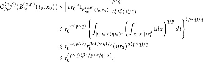 $$ \begin{align*} C^{(\alpha,\beta)}_{p,q}(B^{(\alpha,\beta)}_{r_{0}}(t_{0},x_{0}))&\leq \Big\|cr^{-\alpha}_{0}1_{B^{(\alpha,\beta)}_{r_{0},\eta}(t_{0},x_{0})}\Big\|^{p\wedge q}_{L^{q}_{t}L^{p}_{x}(\mathbb R^{1+n}_{+})}\\ &\lesssim r_{0}^{-\alpha(p\wedge q)}\left\{\int_{|t-t_{0}|<(\eta r_{0})^{\alpha}}\left(\int_{|x-x_{0}|<r^{\beta}_{0}}1dx\right)^{q/p}dt\right\}^{(p\wedge q)/q}\\ &\lesssim r_{0}^{-\alpha(p\wedge q)}r_{0}^{\beta n(p\wedge q)/p}(\eta r_{0})^{\alpha(p\wedge q)/q}\\ &\lesssim r_{0}^{(p\wedge q)(\beta n/p+\alpha/q-\alpha)}.\\[-38pt] \end{align*} $$
3.4 A strong-type inequality related to
$L^{q}_{t}L^{p}_{x}$
-capacity

Theorem 3.8 Given $1\leq p,q<\infty $
,
$1\leq p,q<\infty $
, $\alpha>n$
, and
$\alpha>n$
, and $\beta \in (0,1)$
, for any
$\beta \in (0,1)$
, for any $g\in L^{q}_{t}L^{p}_{x}(\mathbb R^{1+n}_{+})$
, we have
$g\in L^{q}_{t}L^{p}_{x}(\mathbb R^{1+n}_{+})$
, we have
 $$ \begin{align*}\int^{\infty}_{0}\lambda^{p\wedge q}C^{(\alpha,\beta)}_{p,q}(E_{\lambda})\frac{d\lambda}{\lambda}\lesssim \|g\|^{p\wedge q}_{L^{q}_{t}L^{p}_{x}(\mathbb R^{1+n}_{+})},\end{align*} $$
where $E_{\lambda }:=\Big \{(t,x)\in \mathbb R^{1+n}_{+}:\ G_{\alpha ,\beta }(g)(t,x)>\lambda \Big \}$
.
$E_{\lambda }:=\Big \{(t,x)\in \mathbb R^{1+n}_{+}:\ G_{\alpha ,\beta }(g)(t,x)>\lambda \Big \}$
.
Proof Without loss of generality, we assume that $\|g\|_{L^{q}_{t}L^{p}_{x}(\mathbb R^{1+n}_{+})}<\infty $
. For fixed
$\|g\|_{L^{q}_{t}L^{p}_{x}(\mathbb R^{1+n}_{+})}<\infty $
. For fixed $g\in L^{q}_{t}L^{p}_{x}(\mathbb R^{1+n}_{+})$
and any
$g\in L^{q}_{t}L^{p}_{x}(\mathbb R^{1+n}_{+})$
and any $K=K_{t}\times K_{x}\subset \mathbb R^{1+n}_{+}$
, define
$K=K_{t}\times K_{x}\subset \mathbb R^{1+n}_{+}$
, define
 $$ \begin{align*}\Phi_{g}(K):=\frac{\|g\mid_{K}\|^{p\wedge q}_{L^{q}_{t}L^{p}_{x}(\mathbb R^{1+n}_{+})}}{\|g\|^{p\wedge q}_{L^{q}_{t}L^{p}_{x}(\mathbb R^{1+n}_{+})}},\end{align*} $$
where
 $$ \begin{align*} \|g\mid_{K}\|_{L^{q}_{t}L^{p}_{x}(\mathbb R^{1+n}_{+})}&:= \Bigg\{\int_{K_{t}}\Bigg(\int_{K_{x}}|g(t,x)|^{p}dx\Bigg)^{q/p}dt\Bigg\}^{1/q}\\ &= \Bigg\{\int_{0}^{\infty}\Bigg(\int_{\mathbb R^{n}}|g(t,x)|^{p}\chi_{K_{x}}(x)dx\Bigg)^{q/p}\chi_{K_{t}}(t)dt\Bigg\}^{1/q}. \end{align*} $$
For any disjoint sets A and B, it follows from the identity $\chi _{A\cup B}(t,x)=\chi _{A_{t}}(t)\chi _{A_{x}}(x)+\chi _{B_{t}}(t)\chi _{B_{x}}(x)$
that
$\chi _{A\cup B}(t,x)=\chi _{A_{t}}(t)\chi _{A_{x}}(x)+\chi _{B_{t}}(t)\chi _{B_{x}}(x)$
that
 $$ \begin{align*} &\|g\mid_{A\cup B}\|_{L^{q}_{t}L^{p}_{x}(\mathbb R^{1+n}_{+})} \\&\quad\leq \Bigg\{\int_{A_{t}}\Bigg(\int_{A_{x}}|g(t,x)|^{p}dx\Bigg)^{q/p}dt\Bigg\}^{1/q}+ \Bigg\{\int_{B_{t}}\Bigg(\int_{B_{x}}|g(t,x)|^{p}dx\Bigg)^{q/p}dt\Bigg\}^{1/q}\\ &\quad\leq \|g\mid_{A}\|_{L^{q}_{t}L^{p}_{x}(\mathbb R^{1+n}_{+})}+ \|g\mid_{B}\|_{L^{q}_{t}L^{p}_{x}(\mathbb R^{1+n}_{+})}, \end{align*} $$
which means $\Phi _{F}(A\cup B)\leq \Phi _{F}(A)+\Phi _{F}(B)$
. Below, we prove the reverse inequality in two cases.
$\Phi _{F}(A\cup B)\leq \Phi _{F}(A)+\Phi _{F}(B)$
. Below, we prove the reverse inequality in two cases.
Case 1: $p<q$
. For this case,
$p<q$
. For this case, $q/p>1$
. Then we obtain
$q/p>1$
. Then we obtain
 $$ \begin{align*} &\|g\mid_{A\cup B}\|^{p\wedge q}_{L^{q}_{t}L^{p}_{x}(\mathbb R^{1+n}_{+})} \\&\quad= \Bigg\{\int_{(A\cup B)_{t}}\Bigg(\int_{(A\cup B)_{x}}|g(t,x)|^{p}dx\Bigg)^{q/p}dt\Bigg\}^{p/q}\\ &\quad= \Bigg\{\int_{0}^{\infty}\Bigg(\int_{\mathbb R^{n}}|g(t,x)|^{p}\chi_{A\cup B}(t,x)dx\Bigg)^{q/p}dt\Bigg\}^{p/q}\\ &\quad= \Bigg\{\int_{0}^{\infty}\Bigg(\int_{\mathbb R^{n}}|g(t,x)|^{p}\Bigg(\chi_{A}(t,x)+\chi_{B}(t,x)\Bigg)dx\Bigg)^{q/p}dt\Bigg\}^{p/q}\\ &\quad= \Bigg\{\int_{0}^{\infty}\Bigg(\int_{\mathbb R^{n}}|g(t,x)|^{p}\chi_{A}(x,t)dx+\int_{\mathbb R^{n}}|g(t,x)|^{p}\chi_{B}(t,x)dx\Bigg)^{q/p}dt\Bigg\}^{p/q}, \end{align*} $$
which, together with the inequality: $(a+b)^{q/p}\geq a^{q/p}+b^{q/p}, a, b>0$
, implies that
$(a+b)^{q/p}\geq a^{q/p}+b^{q/p}, a, b>0$
, implies that
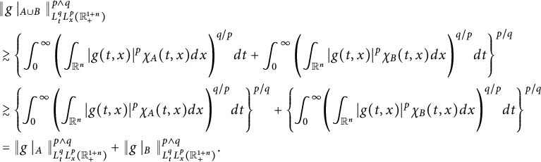 $$ \begin{align*} &\|g\mid_{A\cup B}\|^{p\wedge q}_{L^{q}_{t}L^{p}_{x}(\mathbb R^{1+n}_{+})}\\ &\gtrsim \Bigg\{\!\int_{0}^{\infty}\Bigg(\!\int_{\mathbb R^{n}}|g(t,x)|^{p}\chi_{A}(t,x)dx\Bigg)^{q/p}dt +\int^{\infty}_{0}\Bigg(\!\int_{\mathbb R^{n}}|g(t,x)|^{p}\chi_{B}(t,x)dx\Bigg)^{q/p}dt\Bigg\}^{p/q}\\ &\gtrsim \Bigg\{\!\kern-1pt\int_{0}^{\infty}\Bigg(\!\kern-1pt\int_{\mathbb R^{n}}|g(t,x)|^{p}\chi_{A}(t,x)dx\Bigg)^{q/p}dt\Bigg\}^{p/q} +\Bigg\{\!\kern-1pt\int^{\infty}_{0}\!\Bigg(\!\int_{\mathbb R^{n}}|g(t,x)|^{p}\chi_{B}(t,x)dx\Bigg)^{q/p}dt\Bigg\}^{p/q}\\ &=\|g\mid_{A}\|^{p\wedge q}_{L^{q}_{t}L^{p}_{x}(\mathbb R^{1+n}_{+})}+\|g\mid_{B}\|^{p\wedge q}_{L^{q}_{t}L^{p}_{x}(\mathbb R^{1+n}_{+})}. \end{align*} $$
Case 2: $p\geq q$
. For this case,
$p\geq q$
. For this case, $p\wedge q=q$
. Then
$p\wedge q=q$
. Then
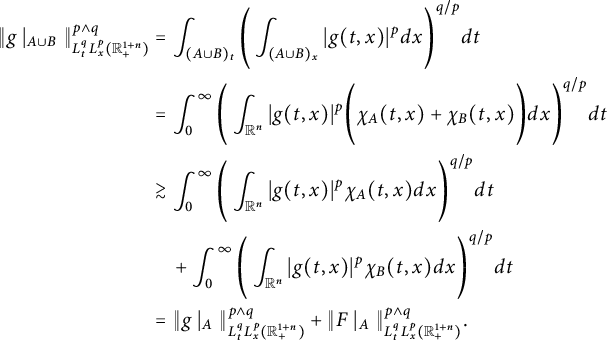 $$ \begin{align*} \|g\mid_{A\cup B}\|^{p\wedge q}_{L^{q}_{t}L^{p}_{x}(\mathbb R^{1+n}_{+})} &= \int_{(A\cup B)_{t}}\Bigg(\int_{(A\cup B)_{x}}|g(t,x)|^{p}dx\Bigg)^{q/p}dt\\ &= \int_{0}^{\infty}\Bigg(\int_{\mathbb R^{n}}|g(t,x)|^{p}\Bigg(\chi_{A}(t,x)+\chi_{B}(t,x)\Bigg)dx\Bigg)^{q/p}dt\\ &\gtrsim \int_{0}^{\infty}\Bigg(\int_{\mathbb R^{n}}|g(t,x)|^{p}\chi_{A}(t,x)dx\Bigg)^{q/p}dt\\ &\quad +\int_{0}^{\infty}\Bigg(\int_{\mathbb R^{n}}|g(t,x)|^{p}\chi_{B}(t,x)dx\Bigg)^{q/p}dt\\ &= \|g\mid_{A}\|^{p\wedge q}_{L^{q}_{t}L^{p}_{x}(\mathbb R^{1+n}_{+})}+\|F\mid_{A}\|^{p\wedge q}_{L^{q}_{t}L^{p}_{x}(\mathbb R^{1+n}_{+})}. \end{align*} $$
Finally, we prove that
 $$ \begin{align*} \Phi_{g}(A\cup B)\simeq \Phi_{g}(A)+\Phi_{g}(B). \end{align*} $$
By [Reference Cerdá, Martín and Silvestre14, Corollary 2.3, p. 187], there exists a measure $\psi $
on
$\psi $
on $\mathbb R^{1+n}_{+}$
such that
$\mathbb R^{1+n}_{+}$
such that $\Phi \leq \psi $
and
$\Phi \leq \psi $
and $\psi (\mathbb R^{1+n}_{+})\leq c(n)$
, where
$\psi (\mathbb R^{1+n}_{+})\leq c(n)$
, where $c(n)$
is a constant only depending on n. For
$c(n)$
is a constant only depending on n. For $E_{\lambda }\setminus E_{a\lambda }$
with
$E_{\lambda }\setminus E_{a\lambda }$
with $a\in (1,2)$
, noting that
$a\in (1,2)$
, noting that $E_{\infty }=\emptyset $
, we have
$E_{\infty }=\emptyset $
, we have
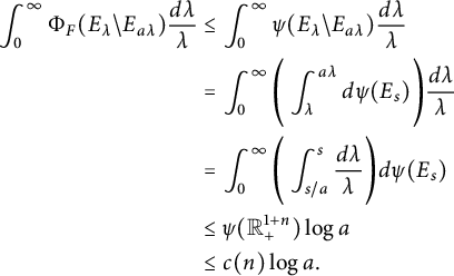 $$ \begin{align*} \int^{\infty}_{0}\Phi_{F}(E_{\lambda}\setminus E_{a\lambda})\frac{d\lambda}{\lambda}&\leq \int^{\infty}_{0}\psi(E_{\lambda}\setminus E_{a\lambda})\frac{d\lambda}{\lambda}\\ &= \int^{\infty}_{0}\Bigg(\int^{a\lambda}_{\lambda}d\psi(E_{s})\Bigg)\frac{d\lambda}{\lambda}\\ &= \int^{\infty}_{0}\Bigg(\int^{s}_{s/a}\frac{d\lambda}{\lambda}\Bigg)d\psi(E_{s})\\ &\leq \psi(\mathbb R^{1+n}_{+})\log a\\ &\leq c(n)\log a. \end{align*} $$
Thus,
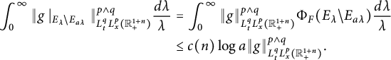 $$ \begin{align*} \int^{\infty}_{0}\|g\mid_{E_{\lambda}\setminus E_{a\lambda}}\|^{p\wedge q}_{L^{q}_{t}L^{p}_{x}(\mathbb R^{1+n}_{+})}\frac{d\lambda}{\lambda} &= \int^{\infty}_{0}\|g\|^{p\wedge q}_{L^{q}_{t}L^{p}_{x}(\mathbb R^{1+n}_{+})}\Phi_{F}(E_{\lambda}\setminus E_{a\lambda})\frac{d\lambda}{\lambda}\\&\leq c(n)\log a \|g\|^{p\wedge q}_{L^{q}_{t}L^{p}_{x}(\mathbb R^{1+n}_{+})}. \end{align*} $$
By (1.3), $u(t,x):=G_{\alpha ,\beta }(g)(t,x)$
is a solution to the space–time fractional dissipative equation:
$u(t,x):=G_{\alpha ,\beta }(g)(t,x)$
is a solution to the space–time fractional dissipative equation:
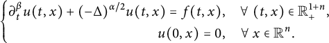 $$ \begin{align*}\left\{\begin{aligned} \partial^{\beta}_{t}u(t,x)+(-\Delta)^{\alpha/2}u(t,x)=f(t,x),&\quad \forall\ (t,x)\in\mathbb R^{1+n}_{+},\\ u(0,x)=0,&\quad \forall\ x\in\mathbb R^{n}. \end{aligned}\right.\end{align*} $$
Set a function $\widetilde {g}$
as
$\widetilde {g}$
as
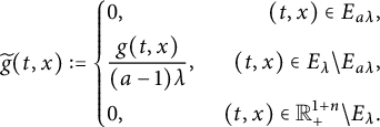 $$ \begin{align*}\widetilde{g}(t,x):=\left\{\begin{aligned} &0,\ &(t,x)\in E_{a\lambda},\\ &\frac{g(t,x)}{(a-1)\lambda},\ &(t,x)\in E_{\lambda}\setminus E_{a\lambda},\\ &0,\ &(t,x)\in \mathbb R^{1+n}_{+}\setminus E_{\lambda}. \end{aligned}\right.\end{align*} $$
Define $\widetilde {f}(t,x)=I^{1-\beta }_{t}\widetilde {g}(t,x).$
Then a direct computation indicates that the following function
$\widetilde {f}(t,x)=I^{1-\beta }_{t}\widetilde {g}(t,x).$
Then a direct computation indicates that the following function
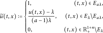 $$ \begin{align*}\widetilde{u}(t,x):=\left\{\begin{aligned} &1,\ &(t,x)\in E_{a\lambda},\\ &\frac{u(t,x)-\lambda}{(a-1)\lambda},\ &(t,x)\in E_{\lambda}\setminus E_{a\lambda},\\ &0,\ &(t,x)\in \mathbb R^{1+n}_{+}\setminus E_{\lambda} \end{aligned}\right.\end{align*} $$
is a solution to the equation
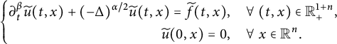 $$ \begin{align*}\left\{\begin{aligned} \partial^{\beta}_{t}\widetilde{u}(t,x)+(-\Delta)^{\alpha/2}\widetilde{u}(t,x)=\widetilde{f}(t,x),&\quad \forall\ (t,x)\in\mathbb R^{1+n}_{+},\\ \widetilde{u}(0,x)=0,&\quad \forall\ x\in\mathbb R^{n}. \end{aligned}\right.\end{align*} $$
Based on the definition of $C^{(\alpha ,\beta )}_{p,q}(\cdot )$
, we obtain
$C^{(\alpha ,\beta )}_{p,q}(\cdot )$
, we obtain
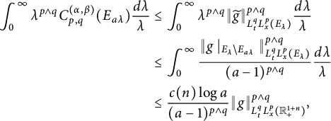 $$ \begin{align*} \int^{\infty}_{0}\lambda^{p\wedge q}C^{(\alpha,\beta)}_{p,q}(E_{a\lambda})\frac{d\lambda}{\lambda}&\leq \int^{\infty}_{0}\lambda^{p\wedge q}\|\widetilde{g}\|^{p\wedge q}_{L^{q}_{t}L^{p}_{x}(E_{\lambda})}\frac{d\lambda}{\lambda}\\ &\leq \int^{\infty}_{0}\frac{\|g\mid_{E_{\lambda}\setminus E_{a\lambda}}\|^{p\wedge q}_{L^{q}_{t}L^{p}_{x}(E_{\lambda})}}{(a-1)^{p\wedge q}}\frac{d\lambda}{\lambda}\\ &\leq \frac{c(n)\log a}{(a-1)^{p\wedge q}} \|g\|^{p\wedge q}_{L^{q}_{t}L^{p}_{x}(\mathbb R^{1+n}_{+})}, \end{align*} $$
which, via a change of variables, implies that
 $$ \begin{align*} \int^{\infty}_{0}\lambda^{p\wedge q}C^{(\alpha,\beta)}_{p,q}(E_{\lambda})\frac{d\lambda}{\lambda}\lesssim \|g\|^{p\wedge q}_{L^{q}_{t}L^{p}_{x}(\mathbb R^{1+n}_{+})}.\\[-42pt] \end{align*} $$
The following weak-type estimate is an immediate corollary of Theorem 3.8.
Corollary 3.9 Let $1\leq p,q<\infty $
,
$1\leq p,q<\infty $
, $\alpha>n$
, and
$\alpha>n$
, and $\beta \in (0,1)$
. For all
$\beta \in (0,1)$
. For all $\lambda>0$
, it holds
$\lambda>0$
, it holds
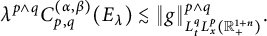 $$ \begin{align*} \lambda^{p\wedge q}C^{(\alpha,\beta)}_{p,q}(E_{\lambda})\lesssim \|g\|^{p\wedge q}_{L^{q}_{t}L^{p}_{x}(\mathbb R^{1+n}_{+})}. \end{align*} $$
As an application of Theorem 3.8, we deduce the embedding from $L^{q}_{t}L^{p}_{x}(\mathbb R^{1+n}_{+})$
to
$L^{q}_{t}L^{p}_{x}(\mathbb R^{1+n}_{+})$
to $L^{(r,s)}(\mathbb R^{1+n}_{+},\mu )$
, which is the Lorentz space of all functions
$L^{(r,s)}(\mathbb R^{1+n}_{+},\mu )$
, which is the Lorentz space of all functions $u(\cdot ,\cdot )$
satisfying
$u(\cdot ,\cdot )$
satisfying
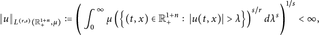 $$ \begin{align*} \|u\|_{L^{(r,s)}(\mathbb R^{1+n}_{+},\mu)}:=\Bigg(\int^{\infty}_{0}\mu\left(\Big\{(t,x)\in\mathbb R^{1+n}_{+}:\ |u(t,x)|>\lambda\Big\}\right)^{s/r}d\lambda^{s}\Bigg)^{1/s}<\infty, \end{align*} $$
where $r,s\in (0,\infty )$
and
$r,s\in (0,\infty )$
and $\mu $
is a nonnegative Borel measure on
$\mu $
is a nonnegative Borel measure on $\mathbb R^{1+n}_{+}$
.
$\mathbb R^{1+n}_{+}$
.
Theorem 3.10 Assume that $1\leq p,q<\infty $
,
$1\leq p,q<\infty $
, $\alpha>n$
, and
$\alpha>n$
, and $\beta \in (0,1)$
. Let
$\beta \in (0,1)$
. Let $\mu $
be a nonnegative Borel measure on
$\mu $
be a nonnegative Borel measure on $\mathbb R^{1+n}_{+}$
. Then
$\mathbb R^{1+n}_{+}$
. Then
 $$ \begin{align} \|G_{\alpha,\beta}(g)\|_{L^{(p\vee q, p\wedge q)}(\mathbb R^{1+n}_{+},\mu)}\lesssim \|g\|_{L^{q}_{t}L^{p}_{x}(\mathbb R^{1+n}_{+})} \end{align} $$
holds for all $g\in L^{q}_{t}L^{p}_{x}(\mathbb R^{1+n}_{+})$
if and only if
$g\in L^{q}_{t}L^{p}_{x}(\mathbb R^{1+n}_{+})$
if and only if
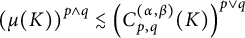 $$ \begin{align} \left(\mu(K)\right)^{p\wedge q}\lesssim \left(C^{(\alpha,\beta)}_{p,q}(K)\right)^{p\vee q} \end{align} $$
holds for all compact sets $K\subset \mathbb R^{1+n}_{+}$
.
$K\subset \mathbb R^{1+n}_{+}$
.
Proof Assume that (3.4) holds. Then it follows from Theorem 3.8 that
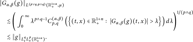 $$ \begin{align*} &\|G_{\alpha,\beta}(g)\|_{L^{(p\vee q, p\wedge q)}(\mathbb R^{1+n}_{+},\mu)} \\&\quad\lesssim \Bigg(\int^{\infty}_{0}\lambda^{p\wedge q-1}C^{(\alpha,\beta)}_{p,q}\left(\Big\{(t,x)\in\mathbb R^{1+n}_{+}:\ |G_{\alpha,\beta}(g)(t,x)|>\lambda\Big\}\right)d\lambda\Bigg)^{1/(p\wedge q)}\\ &\quad\lesssim \|g\|_{L^{q}_{t}L^{p}_{x}(\mathbb R^{1+n}_{+})}. \end{align*} $$
Conversely, suppose that (3.3) holds for all $g\in L^{q}_{t}L^{p}_{x}(\mathbb R^{1+n}_{+})$
. Fix a compact set
$g\in L^{q}_{t}L^{p}_{x}(\mathbb R^{1+n}_{+})$
. Fix a compact set $K\subset \mathbb R^{1+n}_{+}$
. By the definition of
$K\subset \mathbb R^{1+n}_{+}$
. By the definition of $C^{(\alpha ,\beta )}_{p,q}(\cdot )$
, for any
$C^{(\alpha ,\beta )}_{p,q}(\cdot )$
, for any $\epsilon>0$
, there exists a function
$\epsilon>0$
, there exists a function $g\in L^{q}_{t}L^{p}_{x}(\mathbb R^{1+n}_{+})$
such that
$g\in L^{q}_{t}L^{p}_{x}(\mathbb R^{1+n}_{+})$
such that
 $$ \begin{align*}\left\{\begin{aligned} &G_{\alpha,\beta}(g)\geq 1_{K},\\ &\|g\|^{p\wedge q}_{L^{q}_{t}L^{p}_{x}(\mathbb R^{1+n}_{+})}+\epsilon<C^{(\alpha,\beta)}_{p,q}(K). \end{aligned}\right.\end{align*} $$
Hence, $K\subset \Big \{(t,x)\in \mathbb R^{1+n}_{+}:\ |G_{\alpha ,\beta }(g)(t,x)|>1\Big \}$
. We get
$K\subset \Big \{(t,x)\in \mathbb R^{1+n}_{+}:\ |G_{\alpha ,\beta }(g)(t,x)|>1\Big \}$
. We get
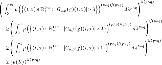 $$ \begin{align*} &\Bigg(\int^{\infty}_{0}\mu\left(\Big\{(t,x)\in\mathbb R^{1+n}_{+}:\ |G_{\alpha,\beta}(g)(t,x)|>\lambda\Big\}\right)^{(p\wedge q)/(p\vee q)}d\lambda^{p\wedge q}\Bigg)^{1/(p\wedge q)}\\ &\quad\geq \Bigg(\int^{1}_{0}\mu\left(\Big\{(t,x)\in\mathbb R^{1+n}_{+}:\ |G_{\alpha,\beta}(g)(t,x)|>\lambda\Big\}\right)^{(p\wedge q)/(p\vee q)}d\lambda^{p\wedge q}\Bigg)^{1/(p\wedge q)}\\ &\quad\geq \Bigg(\int^{1}_{0}\mu\left(\Big\{(t,x)\in\mathbb R^{1+n}_{+}:\ |G_{\alpha,\beta}(g)(t,x)|>1\Big\}\right)^{(p\wedge q)/(p\vee q)}d\lambda^{p\wedge q}\Bigg)^{1/(p\wedge q)}\\ &\quad\geq \left(\mu(K)\right)^{1/(p\vee q)}, \end{align*} $$
which implies that
 $$ \begin{align*} \left(\mu(K)\right)^{(p\wedge q)/(p\vee q)} \leq \|G_{\alpha,\beta}(g)\|^{p\wedge q}_{L^{(p\vee q, p\wedge q)}(\mathbb R^{1+n}_{+},\mu)} \lesssim \|g\|^{p\wedge q}_{L^{q}_{t}L^{p}_{x}(\mathbb R^{1+n}_{+})} \lesssim C^{(\alpha,\beta)}_{p,q}(K)-\epsilon. \end{align*} $$
Then (3.4) follows from the arbitrariness of $\epsilon $
. This completes the proof of Theorem 3.10.
$\epsilon $
. This completes the proof of Theorem 3.10.
4 Hausdorff dimension of the blow-up set
In this section, we estimate the size of the blow-up set of the so-called fractional time–space dissipative potential $G_{\alpha ,\beta }$
: for
$G_{\alpha ,\beta }$
: for $0\leq g\in L^{q}_{t}L^{p}_{x}(\mathbb R^{1+n}_{+})$
,
$0\leq g\in L^{q}_{t}L^{p}_{x}(\mathbb R^{1+n}_{+})$
,
 $$ \begin{align*} \mathcal{B}[G_{\alpha,\beta}(g), p,q]:=\Big\{(t,x)\in\mathbb R^{1+n}_{+}:\ G_{\alpha,\beta}(g)(t,x)=\infty\Big\}. \end{align*} $$
Let $\phi : [0,\infty )\mapsto [0,\infty ]$
be an increasing function with
$\phi : [0,\infty )\mapsto [0,\infty ]$
be an increasing function with $\phi (0)=0$
. For any compact subset
$\phi (0)=0$
. For any compact subset $K\subset \mathbb R^{1+n}_{+}$
, let
$K\subset \mathbb R^{1+n}_{+}$
, let
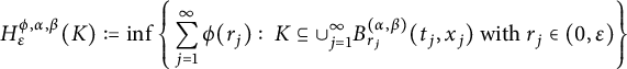 $$ \begin{align*} H^{\phi,\alpha,\beta}_{\epsilon}(K):=\inf\Bigg\{\sum^{\infty}_{j=1}\phi(r_{j}):\ K\subseteq\cup^{\infty}_{j=1}B^{(\alpha,\beta)}_{r_{j}}(t_{j}, x_{j}) \text{ with }r_{j}\in(0,\epsilon)\Bigg\} \end{align*} $$
be the $L^{\alpha ,\beta }$
-based
$L^{\alpha ,\beta }$
-based $(\phi ,\epsilon )$
-Hausdorff capacity of K. Specially, for
$(\phi ,\epsilon )$
-Hausdorff capacity of K. Specially, for $\epsilon =\infty $
,
$\epsilon =\infty $
,
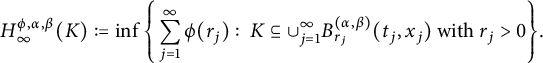 $$ \begin{align*} H^{\phi,\alpha,\beta}_{\infty}(K):=\inf\Bigg\{\sum^{\infty}_{j=1}\phi(r_{j}):\ K\subseteq\cup^{\infty}_{j=1}B^{(\alpha,\beta)}_{r_{j}}(t_{j}, x_{j}) \text{ with }r_{j}>0\Bigg\}. \end{align*} $$
Then the $(\phi ,\epsilon )$
-Hausdorff measure of K is defined by
$(\phi ,\epsilon )$
-Hausdorff measure of K is defined by
 $$ \begin{align*} H^{\phi,\alpha,\beta}(K):=\lim_{\epsilon\rightarrow0}H^{\phi,\alpha,\beta}_{\epsilon}(K). \end{align*} $$
If $\phi (r)=r^{d}$
for all
$\phi (r)=r^{d}$
for all $r\in (0,\infty )$
, then
$r\in (0,\infty )$
, then
 $$ \begin{align*}\left\{\begin{aligned} &H^{\phi,\alpha,\beta}_{\epsilon}(K):=H^{d,\alpha,\beta}_{\epsilon}(K),\\ &H^{\phi,\alpha,\beta}_{\infty}(K):=H^{d,\alpha,\beta}_{\infty}(K),\\ &H^{\phi,\alpha,\beta}(K):=H^{d,\alpha,\beta}(K). \end{aligned}\right.\end{align*} $$
The Hausdorff dimension of K is defined as
 $$ \begin{align*} \text{dim}^{(\alpha,\beta)}_{H}(K):=\inf\Big\{d:\ H^{d,\alpha,\beta}(K)=0\Big\}. \end{align*} $$
Theorem 4.1 $\mathscr {L}^{1}(A)$
and
$\mathscr {L}^{1}(A)$
and $\mathscr {L}^{n}(B)$
stand for the one-dimensional and n-dimensional Lebesgue measures of bounded Borel sets
$\mathscr {L}^{n}(B)$
stand for the one-dimensional and n-dimensional Lebesgue measures of bounded Borel sets $A\subset \mathbb R_{+}$
and
$A\subset \mathbb R_{+}$
and $B\subset \mathbb R^{n}$
, respectively. If
$B\subset \mathbb R^{n}$
, respectively. If $\alpha>n$
,
$\alpha>n$
, $\beta \in (0,1)$
,
$\beta \in (0,1)$
,
 $$ \begin{align*}\left\{\begin{aligned} &1\leq p<\widetilde{p}<\infty,\\ &1<q<\widetilde{q}<\infty,\\ &(1/q-1/\widetilde{q})+n\beta(1/p-1/\widetilde{p})/\alpha=1, \end{aligned}\right.\end{align*} $$
then there exists a $\delta \in (0,1)$
such that
$\delta \in (0,1)$
such that
 $$ \begin{align*}(\mathscr{L}^{1}(A))^{{(p\wedge q)}/{\widetilde{q}}}(\mathscr{L}^{n}(B))^{{(p\wedge q)}/{\widetilde{p}}}\lesssim C^{(\alpha,\beta)}_{p,q}(A\times B)\lesssim H^{(p\wedge q)(n\beta/p+\alpha/q-\alpha),\alpha,\beta}_{\delta}(A\times B).\end{align*} $$
Proof For any $0\leq F$
such that
$0\leq F$
such that $G_{\alpha ,\beta }(g)\geq 1_{A\times B}$
, we can get
$G_{\alpha ,\beta }(g)\geq 1_{A\times B}$
, we can get
 $$ \begin{align*} \|G_{\alpha,\beta}(g)\|_{L^{\widetilde{q}}((0,\infty)), L^{\widetilde p}} &= \Bigg\{\int^{\infty}_{0}\Bigg(\int_{\mathbb R^{n}}|G_{\alpha,\beta}(g)(t,x)|^{\widetilde{p}}dx\Bigg)^{\tilde{q}/\widetilde{p}}dt\Bigg\}^{1/\widetilde{q}}\\&\gtrsim (\mathscr{L}^{1}(A))^{{1}/{\widetilde{q}}}(\mathscr{L}^{n}(B))^{{1}/{\widetilde{p}}}. \end{align*} $$
On the other hand, it follows from Theorem 2.6 that
 $$ \begin{align*} \|G_{\alpha,\beta}(g)\|_{L^{\widetilde{q}}((0,\infty)), L^{\widetilde p}}\lesssim \|g\|_{L^{q}((0,\infty), L^{p})}, \end{align*} $$
which implies
 $$ \begin{align} (\mathscr{L}^{1}(A))^{{(p\wedge q)}/{\widetilde{q}}}(\mathscr{L}^{n}(B))^{{(p\wedge q)}/{\widetilde{p}}}\lesssim \|g\|^{p\wedge q}_{L^{q}((0,\infty), L^{p})}. \end{align} $$
Taking the infimum on the right-hand side of (4.1), we obtain
 $$ \begin{align*} (\mathscr{L}^{1}(A))^{{(p\wedge q)}/{\widetilde{q}}}(\mathscr{L}^{n}(B))^{{(p\wedge q)}/{\widetilde{p}}}\lesssim C^{(\alpha,\beta)}_{p,q}(A\times B). \end{align*} $$
Let $\Big \{B^{(\alpha ,\beta )}_{r_{j}}(t_{j}, x_{j})\Big \}$
be a covering of
$\Big \{B^{(\alpha ,\beta )}_{r_{j}}(t_{j}, x_{j})\Big \}$
be a covering of $A\times B$
with
$A\times B$
with $r_{j}\in (0,\delta )$
. Then, by Theorem 3.7, we get
$r_{j}\in (0,\delta )$
. Then, by Theorem 3.7, we get
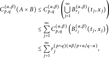 $$ \begin{align*} C^{(\alpha,\beta)}_{p,q}(A\times B)&\leq C^{(\alpha,\beta)}_{p,q}\left(\bigcup^{\infty}_{j=1}B^{(\alpha,\beta)}_{r_{j}}(t_{j}, x_{j})\right)\\ &\leq \sum^{\infty}_{j=1}C^{(\alpha,\beta)}_{p,q}\left(B^{(\alpha,\beta)}_{r_{j}}(t_{j}, x_{j})\right)\\ &\lesssim \sum^{\infty}_{j=1} r_{j}^{(p\wedge q)(n\beta/p+\alpha/q-\alpha)}, \end{align*} $$
which gives
 $$ \begin{align*}C^{(\alpha,\beta)}_{p,q}(A\times B)\lesssim H^{(p\wedge q)(n\beta/p+\alpha/q-\alpha),\alpha,\beta}_{\delta}(A\times B).\end{align*} $$
This completes the proof of Theorem 4.1.
Theorem 4.2 Let K be a compact subset of $\mathbb R^{1+n}_{+}$
. If
$\mathbb R^{1+n}_{+}$
. If $\alpha>n$
,
$\alpha>n$
, $\beta \in (0,1)$
,
$\beta \in (0,1)$
,
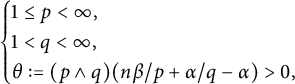 $$ \begin{align*}\begin{cases} 1\leq p<\infty,\\ 1<q<\infty,\\ \theta:=(p\wedge q)(n\beta/p+\alpha/q-\alpha)>0, \end{cases}\end{align*} $$
there exists a $\delta \in (0,1)$
such that
$\delta \in (0,1)$
such that $C^{(\alpha ,\beta )}_{p,q}(K)\lesssim H^{\theta ,\alpha ,\beta }_{\delta }(K)$
and hence
$C^{(\alpha ,\beta )}_{p,q}(K)\lesssim H^{\theta ,\alpha ,\beta }_{\delta }(K)$
and hence
 $$ \begin{align*}\mathrm{dim}_{H}^{(\alpha,\beta)}\left(\mathcal{B}[G_{\alpha,\beta}(g), p,q]\right)\leq n\beta-\alpha(p\wedge q-1).\end{align*} $$
Proof The first assertion follows from Theorem 3.7. Now, we estimate the Hausdorff dimension of the blow-up set. Let $g\geq 0\in L^{q}_{t}L^{p}_{x}(\mathbb R^{1+n}_{+})$
. For any
$g\geq 0\in L^{q}_{t}L^{p}_{x}(\mathbb R^{1+n}_{+})$
. For any $(t,x)\in \mathcal {B}[G_{\alpha ,\beta }(g), p,q]$
,
$(t,x)\in \mathcal {B}[G_{\alpha ,\beta }(g), p,q]$
, $G_{\alpha ,\beta }(g)(t,x)=\infty $
, which means that for
$G_{\alpha ,\beta }(g)(t,x)=\infty $
, which means that for $j\in \mathbb N$
,
$j\in \mathbb N$
, $G_{\alpha ,\beta }(g)(t,x)>2^{j}$
on
$G_{\alpha ,\beta }(g)(t,x)>2^{j}$
on $\mathcal {B}[G_{\alpha ,\beta }(g), p,q]$
. Set
$\mathcal {B}[G_{\alpha ,\beta }(g), p,q]$
. Set $g_{j}=2^{-j}g, j\in \mathbb N$
. Hence,
$g_{j}=2^{-j}g, j\in \mathbb N$
. Hence, $G_{\alpha ,\beta }(g_{j})>1$
on
$G_{\alpha ,\beta }(g_{j})>1$
on $\mathcal {B}[G_{\alpha ,\beta }(g), p,q]$
and
$\mathcal {B}[G_{\alpha ,\beta }(g), p,q]$
and $\|g_{j}\|_{L^{q}_{t}L^{p}_{x}}=2^{-j}\|g\|_{L^{q}_{t}L^{p}_{x}}$
. Then, by the definition of
$\|g_{j}\|_{L^{q}_{t}L^{p}_{x}}=2^{-j}\|g\|_{L^{q}_{t}L^{p}_{x}}$
. Then, by the definition of $C^{(\alpha ,\beta )}_{p,q}(\cdot )$
, it holds
$C^{(\alpha ,\beta )}_{p,q}(\cdot )$
, it holds
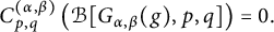 $$ \begin{align*}C^{(\alpha,\beta)}_{p,q}\left(\mathcal{B}[G_{\alpha,\beta}(g), p,q]\right)=0.\end{align*} $$
Let K be any compact subset of $\mathcal {B}[G_{\alpha ,\beta }(g), p,q]$
. By (ii) of Theorem 3.2, we obtain
$\mathcal {B}[G_{\alpha ,\beta }(g), p,q]$
. By (ii) of Theorem 3.2, we obtain $C^{(\alpha ,\beta )}_{p,q}(K)=0$
since
$C^{(\alpha ,\beta )}_{p,q}(K)=0$
since
 $$ \begin{align*}C^{(\alpha,\beta)}_{p,q}(K)\leq C^{(\alpha,\beta)}_{p,q}(\mathcal{B}[G_{\alpha,\beta}(g), p,q]).\end{align*} $$
We need the following Frostman-type lemma: if $\phi : [0,\infty )\mapsto [0,\infty ]$
increases and
$\phi : [0,\infty )\mapsto [0,\infty ]$
increases and $\phi (0)=0$
, then for any given compact
$\phi (0)=0$
, then for any given compact $K\subset \mathbb R^{1+n}_{+}$
, there exists a measure
$K\subset \mathbb R^{1+n}_{+}$
, there exists a measure $\mu \in \mathcal {M}^{+}(K)$
such that
$\mu \in \mathcal {M}^{+}(K)$
such that
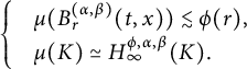 $$ \begin{align*}\begin{cases} &\!\mu(B^{(\alpha,\beta)}_{r}(t,x))\lesssim \phi(r),\\ &\!\mu(K)\simeq H^{\phi,\alpha,\beta}_{\infty}(K). \end{cases}\end{align*} $$
Because K is a compact subset, we assume that K is contained in a ball $B^{(\alpha ,\beta )}_{R}(t_{0},x_{0})$
. Let
$B^{(\alpha ,\beta )}_{R}(t_{0},x_{0})$
. Let $0\leq G\leq L^{q}_{t}L^{p}_{x}(\mathbb R^{1+n}_{+})$
such that
$0\leq G\leq L^{q}_{t}L^{p}_{x}(\mathbb R^{1+n}_{+})$
such that $G_{\alpha ,\beta }(G)\geq 1$
on K. By the Fubini theorem, we get
$G_{\alpha ,\beta }(G)\geq 1$
on K. By the Fubini theorem, we get
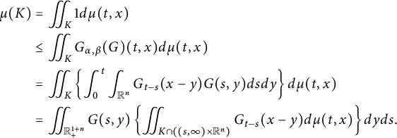 $$ \begin{align*} \mu(K)&= \iint_{K}1d\mu(t,x)\\ &\leq \iint_{K}G_{\alpha,\beta}(G)(t,x)d\mu(t,x)\\ &= \iint_{K}\left\{\int^{t}_{0}\int_{\mathbb R^{n}}G_{t-s}(x-y)G(s,y)dsdy\right\}d\mu(t,x)\\ &= \iint_{\mathbb R^{1+n}_{+}}G(s,y)\left\{\iint_{K\cap ((s,\infty)\times\mathbb R^{n})}G_{t-s}(x-y)d\mu(t,x)\right\}dyds. \end{align*} $$
Applying Proposition 2.1, we obtain
 $$ \begin{align*} \mu(K) \lesssim \iint_{\mathbb R^{1+n}_{+}}G(s,y)\left\{\iint_{K\cap ((s,\infty)\times\mathbb R^{n})}\frac{|t-s|^{\beta}}{(|t-s|^{\beta/\alpha}+|x-y|)^{n+\alpha}}d\mu(t,x)\right\}dyds:= M_{1}+M_{2}, \end{align*} $$
where
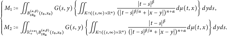 $$ \begin{align*}\left\{\begin{aligned} M_{1}&:=\iint_{B^{(\alpha,\beta)}_{2R_{0}}(t_{0},x_{0})}G(s,y)\left\{\iint_{K\cap ((s,\infty)\times\mathbb R^{n})}\frac{|t-s|^{\beta}}{(|t-s|^{\beta/\alpha}+|x-y|)^{n+\alpha}}d\mu(t,x)\right\}dyds,\\ M_{2}&:=\iint_{\mathbb R^{1+n}_{+}\setminus B^{(\alpha,\beta)}_{2R_{0}}(t_{0},x_{0})}G(s,y)\left\{\iint_{K\cap ((s,\infty)\times\mathbb R^{n})}\frac{|t-s|^{\beta}}{(|t-s|^{\beta/\alpha}+|x-y|)^{n+\alpha}}d\mu(t,x)\right\}dyds. \end{aligned}\right.\end{align*} $$
Now, we estimate the term $M_{2}$
. Write
$M_{2}$
. Write $\mathbb R^{1+n}_{+}\setminus B^{(\alpha ,\beta )}_{2R_{0}}(t_{0},x_{0})\subset S_{1}\cup S_{2}\cup S_{3},$
where
$\mathbb R^{1+n}_{+}\setminus B^{(\alpha ,\beta )}_{2R_{0}}(t_{0},x_{0})\subset S_{1}\cup S_{2}\cup S_{3},$
where
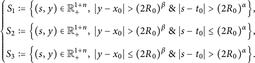 $$ \begin{align*}\left\{\begin{aligned} S_{1}&:=\Big\{(s,y)\in \mathbb R^{1+n}_{+},\ |y-x_{0}|>(2R_{0})^{\beta}\ \&\ |s-t_{0}|>(2R_{0})^{\alpha}\Big\},\\ S_{2}&:=\Big\{(s,y)\in \mathbb R^{1+n}_{+},\ |y-x_{0}|>(2R_{0})^{\beta}\ \&\ |s-t_{0}|\leq(2R_{0})^{\alpha}\Big\},\\ S_{3}&:=\Big\{(s,y)\in \mathbb R^{1+n}_{+},\ |y-x_{0}|\leq(2R_{0})^{\beta}\ \&\ |s-t_{0}|>(2R_{0})^{\alpha}\Big\}. \end{aligned}\right.\end{align*} $$
Hence, $M_{2}\lesssim M_{2,1}+M_{2,2}+M_{2,3}$
, where
$M_{2}\lesssim M_{2,1}+M_{2,2}+M_{2,3}$
, where
 $$ \begin{align*}M_{2,i}:=\iint_{S_{i}}G(s,y)\left\{\iint_{K\cap ((s,\infty)\times\mathbb R^{n})}\frac{|t-s|^{\beta}}{(|t-s|^{\beta/\alpha}+|x-y|)^{n+\alpha}}d\mu(t,x)\right\}dyds,\quad i=1,2,3.\end{align*} $$
For $M_{2,1}$
, if
$M_{2,1}$
, if $(s,y)\in S_{1}$
and
$(s,y)\in S_{1}$
and $(t,x)\in K\cap ((s,\infty )\times \mathbb R^{n})\subset K\subset B^{(\alpha ,\beta )}_{R}(t_{0},x_{0}),$
then
$(t,x)\in K\cap ((s,\infty )\times \mathbb R^{n})\subset K\subset B^{(\alpha ,\beta )}_{R}(t_{0},x_{0}),$
then $|y-x_{0}|\simeq |y-x|$
and
$|y-x_{0}|\simeq |y-x|$
and $|t-s|\simeq |s-t_{0}|$
. We have
$|t-s|\simeq |s-t_{0}|$
. We have
 $$ \begin{align*} \iint_{K\cap ((s,\infty)\times\mathbb R^{n})}\frac{|t-s|^{\beta}}{(|t-s|^{\beta/\alpha}+|x-y|)^{n+\alpha}}d\mu(t,x) \lesssim \frac{|t_{0}-s|^{\beta}}{(|t_{0}-s|^{\beta/\alpha}+|x_{0}-y|)^{n+\alpha}}\mu(K). \end{align*} $$
On the other hand, a direct computation gives
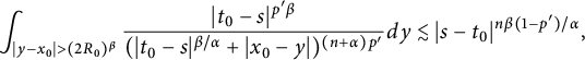 $$ \begin{align*} \int_{|y-x_{0}|>(2R_{0})^{\beta}} \frac{|t_{0}-s|^{p'\beta}}{(|t_{0}-s|^{\beta/\alpha}+|x_{0}-y|)^{(n+\alpha)p'}}dy\lesssim |s-t_{0}|^{n\beta(1-p')/\alpha}, \end{align*} $$
which, together with the Hölder inequality, implies that
 $$ \begin{align*} M_{2,1}&\lesssim \mu(K)\iint_{S_{1}} G(s,y)\frac{|t_{0}-s|^{\beta}}{(|t_{0}-s|^{\beta/\alpha}+|x_{0}-y|)^{n+\alpha}}dyds\\ &\lesssim \mu(K)\|G\|_{L^{q}_{t}L^{p}_{x}(\mathbb R^{1+n}_{+})}\kern-2pt\left\{\kern-2pt\int_{|s-t_{0}|>(2R_{0})^{\alpha}}\kern-1pt\left(\kern-1pt\int_{|y-x_{0}|>(2R_{0})^{\beta}} \kern-1pt\frac{|t_{0}-s|^{p'\beta}}{(|t_{0}-s|^{\beta/\alpha}+|x_{0}-y|)^{(n+\alpha)p'}}dy\kern-1pt\right)^{q'/p'}ds\kern-1pt\right\}^{1/q'}\\ &\lesssim \mu(K)\|G\|_{L^{q}_{t}L^{p}_{x}(\mathbb R^{1+n}_{+})}\left\{\int_{|s-t_{0}|>(2R_{0})^{\alpha}}|s-t_{0}|^{nq'\beta(1-p')/p'\alpha}ds\right\}^{1/q'}\\ &\lesssim \mu(K)\|G\|_{L^{q}_{t}L^{p}_{x}(\mathbb R^{1+n}_{+})}R_{0}^{\alpha-\alpha/q-n\beta/p}. \end{align*} $$
Similarly, for $S_{3}$
, we can see that
$S_{3}$
, we can see that $|t-s|\simeq |s-t_{0}|$
and
$|t-s|\simeq |s-t_{0}|$
and $|t_{0}-s|^{\beta /\alpha }\gtrsim |y-x_{0}|$
. Then
$|t_{0}-s|^{\beta /\alpha }\gtrsim |y-x_{0}|$
. Then
 $$ \begin{align*} \frac{|t-s|^{\beta}}{(|t-s|^{\beta/\alpha}+|x-y|)^{(n+\alpha)}} \lesssim |t_{0}-s|^{\beta-\beta(n+\alpha)/\alpha} \lesssim\frac{|t_{0}-s|^{\beta}}{(|t_{0}-s|^{\beta/\alpha}+|x_{0}-y|)^{n+\alpha}}. \end{align*} $$
We can follow the procedure of $M_{2,1}$
to get
$M_{2,1}$
to get
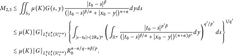 $$ \begin{align*} M_{2,3}&\lesssim \iint_{S_{3}}\mu(K) G(s,y)\frac{|t_{0}-s|^{\beta}}{(|t_{0}-s|^{\beta/\alpha}+|x_{0}-y|)^{n+\alpha}}dyds\\ &\lesssim \mu(K)\|G\|_{L^{q}_{t}L^{p}_{x}(\mathbb R^{1+n}_{+})}\left\{\int_{|s-t_{0}|>(2R_{0})^{\alpha}}\left(\int_{\mathbb R^{n}} \frac{|t_{0}-s|^{p'\beta}}{(|t_{0}-s|^{\beta/\alpha}+|x_{0}-y|)^{(n+\alpha)p'}}dy\right)^{q'/p'}ds\right\}^{1/q'}\\ &\lesssim \mu(K)\|G\|_{L^{q}_{t}L^{p}_{x}(\mathbb R^{1+n}_{+})}R_{0}^{\alpha-\alpha/q-n\beta/p}. \end{align*} $$
Then we estimate $M_{2,2}$
. For
$M_{2,2}$
. For $(s,y)\in S_{2}$
,
$(s,y)\in S_{2}$
, $|y-x_{0}|>|s-t_{0}|^{\beta /\alpha }$
,
$|y-x_{0}|>|s-t_{0}|^{\beta /\alpha }$
, $|y-x_{0}|\simeq |x-y|$
, and
$|y-x_{0}|\simeq |x-y|$
, and $|s-t|\lesssim R^{\alpha }_{0}$
. Then
$|s-t|\lesssim R^{\alpha }_{0}$
. Then
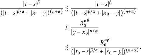 $$ \begin{align*} \frac{|t-s|^{\beta}}{(|t-s|^{\beta/\alpha}+|x-y|)^{(n+\alpha)}}&\lesssim \frac{|t-s|^{\beta}}{(|t-s|^{\beta/\alpha} + |x_{0}-y|)^{(n+\alpha)}}\\ &\lesssim \frac{R_{0}^{\alpha\beta}}{|y-x_{0}|^{n+\alpha}}\\ &\lesssim \frac{R_{0}^{\alpha\beta}}{(|t_{0}-s|^{\beta/\alpha}+|x_{0}-y|)^{(n+\alpha)}}. \end{align*} $$
We can get
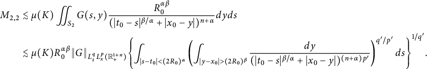 $$ \begin{align*} M_{2,2}&\lesssim \mu(K)\iint_{S_{2}} G(s,y)\frac{R_{0}^{\alpha\beta}}{(|t_{0}-s|^{\beta/\alpha}+|x_{0}-y|)^{n+\alpha}}dyds\\ &\lesssim \mu(K)R^{\alpha\beta}_{0}\|G\|_{L^{q}_{t}L^{p}_{x}(\mathbb R^{1+n}_{+})}\kern-1pt\left\{\kern-1pt\int_{|s-t_{0}|<(2R_{0})^{\alpha}}\left(\kern-1pt\int_{|y-x_{0}|>(2R_{0})^{\beta}} \kern-1pt\frac{dy}{(|t_{0}-s|^{\beta/\alpha}+|x_{0}-y|)^{(n+\alpha)p'}}\kern-1pt\right)^{q'/p'}ds\right\}^{1/q'}\!. \end{align*} $$
The change of variables gives
 $$ \begin{align*} \int_{|y-x_{0}|>(2R_{0})^{\beta}}\frac{1}{(|t_{0}-s|^{\beta/\alpha}+|x_{0}-y|)^{(n+\alpha)p'}}dy\lesssim (|t_{0}-s|^{\beta/\alpha}+|x_{0}-y|)^{-(n+\alpha)p'+n}, \end{align*} $$
which, together with the change of variable: $u=|t_{0}-s|/R^{\alpha }_{0}$
, indicates that
$u=|t_{0}-s|/R^{\alpha }_{0}$
, indicates that
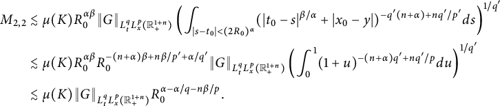 $$ \begin{align*} M_{2,2}&\lesssim \mu(K)R^{\alpha\beta}_{0}\|G\|_{L^{q}_{t}L^{p}_{x}(\mathbb R^{1+n}_{+})}\left(\int_{|s-t_{0}|<(2R_{0})^{\alpha}}(|t_{0}-s|^{\beta/\alpha}+|x_{0}-y|)^{-q'(n+\alpha)+nq'/p'}ds\right)^{1/q'}\\ &\lesssim \mu(K)R^{\alpha\beta}_{0}R_{0}^{-(n+\alpha)\beta+n\beta/p'+\alpha/q'}\|G\|_{L^{q}_{t}L^{p}_{x}(\mathbb R^{1+n}_{+})}\left(\int^{1}_{0}(1+u)^{-(n+\alpha)q'+nq'/p}du\right)^{1/q'}\\ &\lesssim \mu(K)\|G\|_{L^{q}_{t}L^{p}_{x}(\mathbb R^{1+n}_{+})}R_{0}^{\alpha-\alpha/q-n\beta/p}. \end{align*} $$
The estimates for $M_{2,i}, i=1,2,3,$
imply that
$M_{2,i}, i=1,2,3,$
imply that $M_{2}\lesssim \mu (K)\|G\|_{L^{q}_{t}L^{p}_{x}(\mathbb R^{1+n}_{+})}R_{0}^{\alpha -\alpha /q-n\beta /p}.$
Now, we estimate $M_{1}$
. If
$M_{1}$
. If $(s,y)\in B^{(\alpha ,\beta )}_{2R_{0}}(t_{0},x_{0})$
and
$(s,y)\in B^{(\alpha ,\beta )}_{2R_{0}}(t_{0},x_{0})$
and $(t,x)\in B^{(\alpha ,\beta )}_{2R_{0}}(t_{0},x_{0})$
, then
$(t,x)\in B^{(\alpha ,\beta )}_{2R_{0}}(t_{0},x_{0})$
, then $|t-s|<(4R_{0})^{\alpha }$
and
$|t-s|<(4R_{0})^{\alpha }$
and $|y-x|\leq (4R_{0})^{\beta }$
, which indicate that
$|y-x|\leq (4R_{0})^{\beta }$
, which indicate that $(t,x)\in B^{(\alpha ,\beta )}_{4R_{0}}(s,y)$
. We can get
$(t,x)\in B^{(\alpha ,\beta )}_{4R_{0}}(s,y)$
. We can get
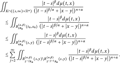 $$ \begin{align*} &\iint_{K\cap ((s,\infty)\times\mathbb R^{n})}\frac{|t-s|^{\beta}d\mu(t,x)}{(|t-s|^{\beta/\alpha}+|x-y|)^{n+\alpha}} \\&\quad\lesssim \iint_{B^{(\alpha,\beta)}_{2R_{0}}(t_{0},x_{0})}\frac{|t-s|^{\beta}d\mu(t,x)}{(|t-s|^{\beta/\alpha}+|x-y|)^{n+\alpha}}\\ &\quad\lesssim \iint_{B^{(\alpha,\beta)}_{4R_{0}}(s,y)}\frac{|t-s|^{\beta}d\mu(t,x)}{(|t-s|^{\beta/\alpha}+|x-y|)^{n+\alpha}}\\ &\quad\lesssim \sum^{\infty}_{j=2}\iint_{B^{(\alpha,\beta)}_{2^{-j}R_{0}}(s,y)\setminus B^{(\alpha,\beta)}_{2^{-j-1}R_{0}}(s,y)}\frac{|t-s|^{\beta}d\mu(t,x)}{(|t-s|^{\beta/\alpha}+|x-y|)^{n+\alpha}}. \end{align*} $$
Let $(t,x)\in B^{(\alpha ,\beta )}_{2^{-j}R_{0}}(s,y)\setminus B^{(\alpha ,\beta )}_{2^{-j-1}R_{0}}(s,y)$
. If
$(t,x)\in B^{(\alpha ,\beta )}_{2^{-j}R_{0}}(s,y)\setminus B^{(\alpha ,\beta )}_{2^{-j-1}R_{0}}(s,y)$
. If $|t-s|\simeq (2^{-j_{0}}R_{0})^{\alpha }$
and
$|t-s|\simeq (2^{-j_{0}}R_{0})^{\alpha }$
and $|x-x_{0}|<(2^{-j_{0}}R_{0})^{\beta }$
, then
$|x-x_{0}|<(2^{-j_{0}}R_{0})^{\beta }$
, then
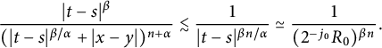 $$ \begin{align*} \frac{|t-s|^{\beta}}{(|t-s|^{\beta/\alpha}+|x-y|)^{n+\alpha}}\lesssim \frac{1}{|t-s|^{\beta n/\alpha}}\simeq \frac{1}{(2^{-j_{0}}R_{0})^{\beta n}}. \end{align*} $$
If $|t-s|< (2^{-j_{0}}R_{0})^{\alpha }$
and
$|t-s|< (2^{-j_{0}}R_{0})^{\alpha }$
and $|x-x_{0}|\simeq (2^{-j_{0}}R_{0})^{\beta }$
, then
$|x-x_{0}|\simeq (2^{-j_{0}}R_{0})^{\beta }$
, then
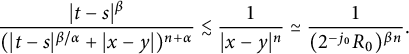 $$ \begin{align*} \frac{|t-s|^{\beta}}{(|t-s|^{\beta/\alpha}+|x-y|)^{n+\alpha}}\lesssim \frac{1}{|x-y|^{n}}\simeq \frac{1}{(2^{-j_{0}}R_{0})^{\beta n}}. \end{align*} $$
We have
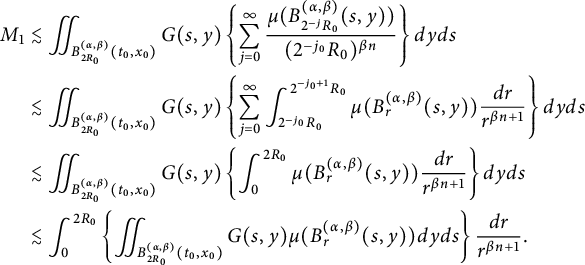 $$ \begin{align*} M_{1}&\lesssim \iint_{B^{(\alpha,\beta)}_{2R_{0}}(t_{0},x_{0})}G(s,y) \left\{\sum^{\infty}_{j=0}\frac{\mu(B^{(\alpha,\beta)}_{2^{-j}R_{0}}(s,y))}{(2^{-j_{0}}R_{0})^{\beta n}}\right\}dyds\\ &\lesssim \iint_{B^{(\alpha,\beta)}_{2R_{0}}(t_{0},x_{0})}G(s,y) \left\{\sum^{\infty}_{j=0}\int^{2^{-j_{0}+1}R_{0}}_{2^{-j_{0}}R_{0}} \mu(B^{(\alpha,\beta)}_{r}(s,y))\frac{dr}{r^{\beta n+1}}\right\}dyds\\ &\lesssim \iint_{B^{(\alpha,\beta)}_{2R_{0}}(t_{0},x_{0})}G(s,y) \left\{\int^{2R_{0}}_{0} \mu(B^{(\alpha,\beta)}_{r}(s,y))\frac{dr}{r^{\beta n+1}}\right\}dyds\\ &\lesssim \int^{2R_{0}}_{0} \left\{\iint_{B^{(\alpha,\beta)}_{2R_{0}}(t_{0},x_{0})}G(s,y)\mu(B^{(\alpha,\beta)}_{r}(s,y))dyds\right\}\frac{dr}{r^{\beta n+1}}. \end{align*} $$
Case 1: $p\leq q$
. Applying Hölder’s inequality, we get
$p\leq q$
. Applying Hölder’s inequality, we get
 $$ \begin{align} &\|G\|_{L^{p}_{t}L^{p}_{x}(B^{(\alpha,\beta)}_{2R_{0}}(t_{0},x_{0}))}\\&\qquad\leq \left\{\int_{|s-t_{0}|<(2R_{0})^{\alpha}}\left(\int_{|y-x_{0}| <(2R_{0})^{\beta}}|G(s,y)|^{p}dy\right)ds\right\}^{1/p}\nonumber\\ &\qquad \lesssim \left\{\int_{|s-t_{0}|<(2R_{0})^{\alpha}} \left(\int_{|y-x_{0}|<(2R_{0})^{\beta}}|G(s,y)|^{p}dy\right)^{q/p}ds\right\}^{1/q}\left(\int_{|s-t_{0}|<(2R_{0})^{\alpha}}1ds\right)^{1/p-1/q}\nonumber\\ &\qquad \lesssim \|G\|_{L^{q}_{t}L^{p}_{x}(\mathbb R^{1+n}_{+})}R_{0}^{\alpha(1/p-1/q)}.\nonumber \end{align} $$
On the other hand, it follows from the condition $\mu (B^{(\alpha ,\beta )}_{r}(s,y))\lesssim \phi (r)$
that
$\mu (B^{(\alpha ,\beta )}_{r}(s,y))\lesssim \phi (r)$
that
 $$ \begin{align} \left(\mu(B^{(\alpha,\beta)}_{r}(s,y))\right)^{p/(p-1)} \lesssim\left(\phi(r)\right)^{1/(p-1)}\mu(B^{(\alpha,\beta)}_{r}(s,y)). \end{align} $$
The estimates (4.2) and (4.3) imply that
 $$ \begin{align*} M_{1}&\lesssim \int^{2R_{0}}_{0}\|G\|_{L^{p}_{t}L^{p}_{x}(B^{(\alpha,\beta)}_{2R_{0}}(t_{0},x_{0}))} \left\{\iint_{B^{(\alpha,\beta)}_{2R_{0}}(t_{0},x_{0})}\left(\mu(B^{(\alpha,\beta)}_{r}(s,y))\right)^{p/(p-1)}dyds\right\}^{1-1/p}\frac{dr}{r^{\beta n+1}}\\ &\lesssim \|G\|_{L^{q}_{t}L^{p}_{x}(\mathbb R^{1+n}_{+})}R_{0}^{\alpha(1/p-1/q)}\int^{2R_{0}}_{0} \left\{\iint_{B^{(\alpha,\beta)}_{2R_{0}}(t_{0},x_{0})} \mu(B^{(\alpha,\beta)}_{r}(s,y))dyds\right\}^{1-1/p}\frac{(\phi(r))^{1/p}dr}{r^{\beta n+1}}. \end{align*} $$
Since $\mu \in \mathcal {M}^{+}(K)$
,
$\mu \in \mathcal {M}^{+}(K)$
, $\mu (B^{(\alpha ,\beta )}_{r}(s,y))\leq \mu (K)$
. For any
$\mu (B^{(\alpha ,\beta )}_{r}(s,y))\leq \mu (K)$
. For any $0<r<2R_{0}$
and
$0<r<2R_{0}$
and $(t,x)\in B^{(\alpha ,\beta )}_{r}(s,y)$
, it holds
$(t,x)\in B^{(\alpha ,\beta )}_{r}(s,y)$
, it holds
 $$ \begin{align*} \iint_{B^{(\alpha,\beta)}_{2R_{0}}(t_{0},x_{0})} \mu(B^{(\alpha,\beta)}_{r}(s,y))dyds &=\iint_{B^{(\alpha,\beta)}_{2R_{0}}(t_{0},x_{0})} \left(\iint_{B^{(\alpha,\beta)}_{r}(s,y)}1d\mu(t,x)\right)dyds\\ &\lesssim\iint_{\mathbb R^{1+n}_{+}}\left(\iint_{B^{(\alpha,\beta)}_{r}}1dyds\right)d\mu(t,x) \lesssim r^{\alpha+\beta n}\mu(K). \end{align*} $$
Hence,
 $$ \begin{align*} M_{1}&\lesssim \|G\|_{L^{q}_{t}L^{p}_{x}(\mathbb R^{1+n}_{+})}R_{0}^{\alpha(1/p-1/q)}\int^{2R_{0}}_{0} \left(r^{\alpha+\beta n}\mu(K)\right)^{1-1/p}\frac{(\phi(r))^{1/p}dr}{r^{\beta n+1}}\\ &\lesssim \|G\|_{L^{q}_{t}L^{p}_{x}(\mathbb R^{1+n}_{+})}R_{0}^{\alpha(1/p-1/q)}\left(\mu(K)\right)^{1-1/p} \int^{2R_{0}}_{0}\left(\phi(r)\right)^{1/p}r^{\alpha(1-1/p)-\beta n/p-1}dr. \end{align*} $$
Case 2: $p>q$
. Similar to Case 1, we have
$p>q$
. Similar to Case 1, we have
 $$ \begin{align*} M_{1}&\lesssim \int^{2R_{0}}_{0} \left\{\iint_{B^{(\alpha,\beta)}_{2R_{0}}(t_{0},x_{0})}G(s,y)\mu(B^{(\alpha,\beta)}_{r}(s,y))dyds\right\}\frac{dr}{r^{1+\beta n}}\\ &\lesssim \|G\|_{L^{q}_{t}L^{q}_{x}(B^{(\alpha,\beta)}_{2R_{0}}(t_{0},x_{0}))}\int^{2R_{0}}_{0} \left(\iint_{B^{(\alpha,\beta)}_{2R_{0}}(t_{0},x_{0})}\left(\mu(B^{(\alpha,\beta)}_{r}(s,y))\right)^{q/(q-1)}dyds\right)^{1-1/q}\frac{dr}{r^{\beta n+1}}\\ &\lesssim R_{0}^{n(1/q-1/p)}\|G\|_{L^{q}_{t}L^{p}_{x}(\mathbb R^{1+n}_{+})}\int^{2R_{0}}_{0} \left(\iint_{B^{(\alpha,\beta)}_{2R_{0}}(t_{0},x_{0})}\mu(B^{(\alpha,\beta)}_{r}(s,y))dyds\right)^{1-1/q}\frac{(\phi(r))^{1/q}dr}{r^{\beta n+1}}\\ &\lesssim R_{0}^{n(1/q-1/p)}\|G\|_{L^{q}_{t}L^{p}_{x}(\mathbb R^{1+n}_{+})}(\mu(K))^{1-1/q}\int^{2R_{0}}_{0}(\phi(r))^{1/q}r^{\alpha(1-1/q)\beta n/q-1}dr. \end{align*} $$
Hence, there exists a constant $c_{0}$
depending on
$c_{0}$
depending on $p,q,\alpha , \beta , R_{0}$
such that
$p,q,\alpha , \beta , R_{0}$
such that
 $$ \begin{align*} \mu(K) \leq c_{0}\|G\|_{L^{q}_{t}L^{p}_{x}(\mathbb R^{1+n}_{+})}\left\{\mu(K)+(\mu(K))^{1-1/(p\wedge q)}\int^{2R_{0}}_{0}(\phi(r))^{1/(p\wedge q)}r^{-1+\alpha-(\alpha+\beta n)/(p\wedge q)}dr\right\}. \end{align*} $$
Take $\phi (r):=r^\eta $
,
$\phi (r):=r^\eta $
, $\eta>n\beta -\alpha (p\wedge q-1)$
, such that
$\eta>n\beta -\alpha (p\wedge q-1)$
, such that
 $$ \begin{align*} \int^{2R_{0}}_{0}(\phi(r))^{1/(p\wedge q)}r^{-1+\alpha-(\alpha+\beta n)/(p\wedge q)}dr<\infty. \end{align*} $$
This gives
 $$ \begin{align*} \frac{(\mu(K))^{1/(p\wedge q)}}{1+(\mu(K))^{1/(p\wedge q)}}\leq c_{0}\|G\|_{L^{q}_{t}L^{p}_{x}(\mathbb R^{1+n}_{+})}, \end{align*} $$
and therefore
 $$ \begin{align*} \frac{(\mu(K))^{1/(p\wedge q)}}{1+(\mu(K))^{1/(p\wedge q)}}\leq c_{0}C^{(\alpha,\beta)}_{p,q}(K)=0, \end{align*} $$
which implies that $\mu (K)=0$
and
$\mu (K)=0$
and $H^{\phi ,\alpha ,\beta }_{\infty }(K)=0$
. Hence,
$H^{\phi ,\alpha ,\beta }_{\infty }(K)=0$
. Hence, $H^{\phi ,\alpha ,\beta }(K)=0$
. By the arbitrariness of
$H^{\phi ,\alpha ,\beta }(K)=0$
. By the arbitrariness of $K\subset \mathcal {B}(G_{\alpha ,\beta }(g),p,q)$
,
$K\subset \mathcal {B}(G_{\alpha ,\beta }(g),p,q)$
,
 $$ \begin{align*} H^{\phi,\alpha,\beta}(\mathcal{B}(G_{\alpha,\beta}(g),p,q))=0, \end{align*} $$
which indicates that
 $$ \begin{align*} \text{dim}_{H}^{(\alpha,\beta)}\left(\mathcal{B}[G_{\alpha,\beta}(g), p,q]\right)\leq n\beta-\alpha(p\wedge q-1).\\[-35pt] \end{align*} $$


 Open access