Physics-constrained machine learning for reduced composition space chemical kinetics

Abstract

Modeling detailed chemical kinetics is a primary challenge in combustion simulations. We present a novel framework to enforce physical constraints, specifically total mass and elemental conservation, during the reaction of ML models’ training for the reduced composition space chemical kinetics of large chemical mechanisms in combustion. In these models, the transport equations for a subset of representative species are solved with the ML approaches, while the remaining nonrepresentative species are “recovered” with a separate artificial neural network trained on data. Given the strong correlation between full and reduced solution vectors, our method utilizes a small neural network to establish an accurate and physically consistent mapping. By leveraging this mapping, we enforce physical constraints in the training process of the ML model for reduced composition space chemical kinetics. The framework is demonstrated here for methane, CH₄, and oxidation. The resulting solution vectors from our deep operator networks (DeepONet)-based approach are accurate and align more consistently with physical laws.

Impact statement

The integration of complex fuel chemistry in practical computational fluid dynamics (CFD) applications requires extensive computational resources. We integrate two machine-learning frameworks to accelerate chemistry integration, reduce the dimensionality of the solution vector, reconstruct the full chemical system, and enforce mass and element conservation. The first framework, React-DeepONet, advances the solution of representative species by mapping it across small time increments. The second framework, Correlation Net, reconstructs the remaining species and implements mass and element conservation to evaluate training loss. The integrated framework reduces the computational cost and memory requirements associated with advancing a full chemical system. At the same time, Correlation Net emulates the output of a full chemical system solution with mass and element conservation constraints.

1. Introduction

The detailed modeling of chemical kinetics is the principal bottleneck in the combustion simulations. Recently, several efforts have been made to learn the chemical kinetics and accelerate its integration in a simulation using machine learning (ML) tools (Blasco et al., 1998, 2000; Haghshenas et al., 2021; Ji and Deng, 2021; Ranade et al., 2019). However, due to the high dimensionality of the chemical systems for complex fuels, the ML models have predominantly been restricted to simpler fuels and mechanisms. For larger and more complex reaction mechanisms that have a high-dimensional solution vector of thermo-chemical scalars, chemical kinetics may be learned in the reduced composition space (Dikeman et al., 2022; Kumar and Echekki, 2024, either through dimensionality reduction techniques by advancing solutions of the chemical system in latent space (see, for example, (Goswami et al., 2024; Kumar and Echekki, 2024) or by transporting a subset of the chemical system through representative species (Kumar and Echekki, 2024.

While ML models have demonstrated significant potential for capturing chemical kinetics in the reduced composition space, the temporal evolution of the reduced solution vector may not conform to certain physical constraints, like total mass and elemental conservation. These physical constraints are typically essential for CFD solvers, potentially hindering the integration of ML models with such solvers.

Recent efforts have explored incorporating domain-specific physical principles or laws into neural network training by adjusting the loss function (Raissi et al., 2019), allowing the models to rely on data and established physical knowledge. An obvious step of incorporating the physical constraint of total mass and elemental conservation in the ML training process for reduced composition space chemical kinetics is hindered by the unavailability of the full solution vector representing all species in a chemical mechanism. Enforcing these constraints during training often requires the recovery of the full solution vector.

In this article, we introduce a framework that enables the implementation of a chemistry acceleration tool based on predicting a subset of species within the chemical system. This subset is referred to as representative species from which other nonrepresentative species can be recovered. Using training data, this framework recovers nonrepresentative species using an artificial neural network (ANN) called Correlation Net and implements mass and element conservation within the loss evaluation.

This framework is readily adaptable to any ML model aiming to capture the chemical kinetics of complex combustion fuels with a subset of the species. However, in this study, we integrate it with the React-DeepONet of Kumar and Echekki (2024). The React-DeepONet architecture is based on deep operator networks (DeepONets) by Lu et al. (2021). React-DeepONet is designed to map a solution vector of a subset of the thermo-chemical scalars, temperature, and representative species at a prescribed time onto a solution at a later small time increment. Representative species are selected because of their role as markers for the evolution of fuel oxidation and their strong correlation with the remaining (nonrepresentative species) (Pope, 2013). Similar approaches using DeepONets, albeit with the integration of the full chemical systems, have been proposed by Venturi and Casey (2023) and Goswami et al. (2024). As in these two approaches, React-DeepONet is trained on simulation data. Its implementation with a reduced set of chemical systems is designed to overcome the challenges of integrating a full thermo-chemical system with stiff ODEs for large and complex fuels. The React-DeepONet-based scheme results in up to three orders of magnitude accelerations in the chemistry prediction of complex fuels (Kumar and Echekki, 2024.

In this study, we first establish a physically consistent mapping from the reduced set of representative species to the full solution vector. Subsequently, we incorporate the physical constraints of total mass and elemental conservation into the training of React-DeepONet, which learns chemical kinetics in a reduced composition space. As a result, the solution vector produced by React-DeepONet achieves greater physical consistency, retaining its predictive accuracy.

2. Methodology

2.1. Chemical kinetics identification through a deep operator network

This section discusses the proposed framework for the physics-informed enforcement of mass and element conservation. As stated earlier, we integrate the framework with our recently developed React-DeepONet framework for chemistry acceleration. The framework is designed to predict the solution of a subset of the thermo-chemical scalars’ vectors between two prescribed time increments. Therefore, the framework is designed to advance the chemical source operator that can be coupled with transport in a CFD simulation. We illustrate the framework using data for a 0D, homogeneous mixture with prescribed pressure, composition (through an equivalence ratio), and initial temperature. The corresponding system of ODEs, which are solved as an initial value problem, takes the form:

(2.1) $$ \frac{d{\phi}_i}{dt}=f(\phi, \hskip.4em {p}_0),\hskip1em i=1,2,3,\dots, n $$

(2.2) $$ \phi (0)={\phi}_0 $$

where $ \phi $ is the thermo-chemical composition vector, which includes species mass fractions and temperature, the chemical source term $ f(\phi, \hskip.4em {p}_0) $ is a function of thermo-chemical scalars, $ \phi $ , and is typically modeled using the law of mass action. The chemical kinetics presented by the above system of stiff ODEs is learned through the React-DeepONet framework of Kumar and Echekki (2024), where a reduced set of representative species is considered instead of the full thermochemical solution vector. This choice yields significant savings in computational time and memory, but accounting for a partial solution of the chemical system must also address mass and element conservation.

The dimensionality of the reduced composition space ( $ {\phi}_i,i=1,2,\dots m\in {R}^m $ ) is far smaller than the dimensionality of the original solution vector ( $ {\phi}_i,i=1,2,\dots m,m+1,m+2,\dots n\in {R}^n $ ). In the Kumar and Echekki study (2024), the React-DeepONet that was used to capture the two-stage ignition process of n-dodecane at various initial conditions was implemented with seven representative species and temperature (i.e., $ m= $ 8), and the full mechanism required the integration of 348 species and temperature (i.e., $ n= $ 349).

It is important to note that for implementing the proposed approach in CFD calculations, the training data should be suitable for the targeted composition space in CFD. This data can be generated using 0D (Nguyen et al., 2021; Mehl and Aubagnac-Karkar, 2023) or 1D (e.g., 1D flamelets) reactors. Simpler 2D or 3D direct numerical simulations or a reduced scale or dimension represent alternatives to construct the targeted composition space (Owoyele and Echekki, 2017; Kumar et al., 2023).

The React-DeepONet architecture adopted by Kumar and Echekki (2024) is shown in Figure 1. It consists of two subnetworks, the Branch Net and the Trunk Net, which include as inputs the solution vector for the representative species and temperature at a time, $ t $ , and a prescribed time step, $ \delta t $ , on the Branch and Trunk nets, respectively. The outputs of the two subnetworks are combined in a concatenation layer, resulting in output for the solution vector for the representative species and temperature at a later time increment, $ t+\delta t $ . Based on its architecture, React-DeepONet maps the solution vector of a set of representative species and temperature at a time of the evolution of this solution across a time step $ \delta t $ , thus avoiding the costly direct chemistry integration and enabling the time step, $ \delta t $ , to be prescribed primarily by transport time scale requirements in reacting flow simulations. To train the React-DeepONet, the following loss function is evaluated, which compares the React-DeepONet predictions to the training data, which corresponds to the numerically integrated solution of the full chemical system:

(2.3) $$ {\mathcal{L}}_{\mathrm{DATA}}=\frac{1}{m}\sum \limits_{i=1}^m{({\phi}_i(t+\delta t)-{\phi}_i^{\ast }(t+\delta t))}^2 $$

where $ \delta t $ varies from $ 0 $ to a large fixed time step $ \Delta t $ and $ {\phi}_i^{\ast}\left(t+\delta t\right) $ is the corresponding ground-truth value. Therefore, React-DeepONet accommodates training for a range of values for $ \delta t $ within $ \Delta t $ . During prediction, any value of $ \delta t $ within this range can be used or adaptively changed during the simulation. The training prescribed above acts as a preconditioner for the model parameters, and additional refined training is implemented based on an autoregressive procedure (Kumar and Echekki, 2024. Within the process, the refined model is trained to predict the solution vector at multiple time steps, $ {N}_l $ . Accordingly, the loss function of the refined training model combines the loss functions corresponding to steps from 1 to N $ {}_l $ .

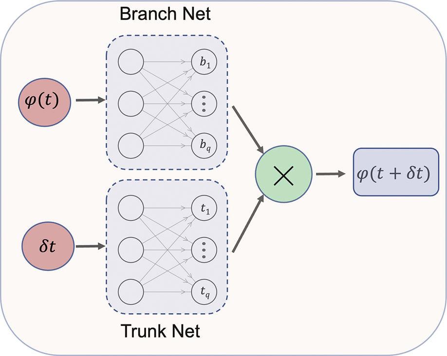
Figure 1. React-DeepONet: ANN for predicting the evolution of representative species and temperature.

2.2. Mapping nonrepresentative species from the reduced set: Correlation Net

The objective of the proposed approach is twofold: (1) to constrain the React-DeepONet predictions to satisfy mass and element conservation and (2) to predict nonrepresentative species, which are not predicted using React-DeepONet or transported in CFD. These species, combined with the representative species, may account for the bulk of the mass in the mixture. Although the dimensionality of the full solution vector is very large, it resides on a low-dimensional manifold since most of the scalars are highly correlated (Pope, 2013; Coussement et al., 2016). The reduced set ( $ {\phi}_i,i=1,2,\dots m $ ), identified based on principal component analysis (PCA) of reaction rate data as proposed by Alqahtani and Echekki (2021), is representative of the thermo-chemical manifold. It strongly correlates with the nonrepresentative species ( $ {\phi}_i,i=m+1,m+2,\dots n $ ). However, other methods for selecting the representative species can be used including directed relations graphs (DRGs) methods (Lu and Law, 2005), the global pathway selection (GPS) algorithm (Gao et al., 2016), or the more recent manifold-informed state vector subset (Zdybał et al., 2023). Recently, we showed that the PCA-based technique and the other three techniques yield similar representative species for chemical systems (Gitushi and Echekki, 2024).

Leveraging their high correlation, nonrepresentative species can be mapped from the reduced set of representative species using an ANN denoted as Correlation Net as shown in Figure 2. The training of the ANNs is implemented using training data from simulations that capture the accessed composition space of the target simulations in CFD. Inputs and outputs to Correlation Net are the representative species and temperature and nonrepresentative species, respectively, as shown in Figure 2. The loss that is evaluated during training is expressed as

(2.4) $$ {\mathrm{\mathcal{L}}}_{\mathrm{C}-\mathrm{DATA}}=\frac{1}{\left(m-n\right)}\sum \limits_{i=m+1}^n{\left({\phi}_i-{\phi}_i^{\ast}\right)}^2 $$

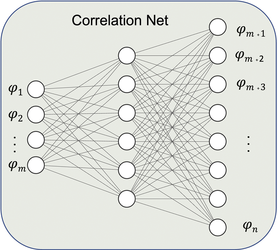
Figure 2. Correlation Net: ANN for recovering nonrepresentative species.

Again, the loss compares predictions by Correlation Net with values obtained from the training data and resulting from the direct integration of the full thermo-chemical scalars’ solution vector. Since the full thermo-chemical space obeys certain physical laws, such as the sum of species mass fractions is one and elements remain conserved during the reaction as the solution vector evolves, Correlation Net is trained with additional losses corresponding to these physical constraints.

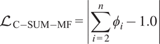(2.5) $$ {\mathrm{\mathcal{L}}}_{\mathrm{C}-\mathrm{SUM}-\mathrm{MF}}=\left|\sum \limits_{i=2}^n{\phi}_i-1.0\right| $$

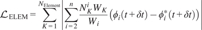
(2.6) $$ {\mathrm{\mathcal{L}}}_{\mathrm{C}-\mathrm{ELEM}}=\sum \limits_{K=1}^{N_{\mathrm{Element}}}\left|\sum \limits_{i=2}^n\frac{N_K^i{W}_K}{W_i}\left({\phi}_i-{\phi}_i^{\ast}\right)\right|, $$

where $ {N}_K^i $ is the Kth element contribution in ith species, $ {W}_K $ is the atomic weight of Kth element, and $ {W}_i $ is the molecular weight of the ith species. Also, $ {\phi}_1 $ is essentially temperature and is excluded from the conservation loss formulations. It should be noted that these two losses include the Correlation Net output and its input. The total loss function for Correlation Net takes this form:

(2.7) $$ {\mathrm{\mathcal{L}}}_C={W}_1\;{\mathrm{\mathcal{L}}}_{\mathrm{C}-\mathrm{DATA}}+{W}_2\;{\mathrm{\mathcal{L}}}_{\mathrm{C}-\mathrm{SUM}-\mathrm{MF}}+{W}_3\;{\mathrm{\mathcal{L}}}_{\mathrm{C}-\mathrm{ELEM}}, $$

which combines losses associated with correlations and mass and element conservation. In this expression, $ {W}_1 $ , $ {W}_2 $ , and $ {W}_3 $ are the weights for each loss term. The choice of the weights is dictated by the magnitudes of the various loss terms within Eq. (2.7) as discussed below. Although mass and element conservation may be redundant for reactions, they represent two useful constraints to enforce during the Correlation Net training. The results discussed below will investigate whether implementing both constraints improves the training of Correlation Net.

It is important to note that alternative approaches have been developed in the literature to reinforce mass and element conservation within the framework of ANN-based predictions of chemistry. Readshaw et al. (2023) implemented mass conservation in different steps. In the first step, the species are predicted by training an ANN without mass conservation constraints. The subsequent steps are implemented outside the ANN predictions. In these steps, residual species representing the main contributions to the elements are determined based on the ANN predictions. Then, the mass fractions of these species are recalculated to conserve their corresponding elements across the integration time step. An additional step is implemented if the new value of the residual species is negative by setting its value to zero and enforcing element conservation using two rectifying species.

Mehl and Aubagnac-Karkar (2023) also adopted a correction scheme for element conservation on selected species. For H₂ oxidation, H and O elements are corrected by adding to or removing mass from H₂ and O₂ from the ANN predictions. They also implemented an element-based hybrid model to replace the ANN evaluation with direct integration predictions when an error proxy exceeded a threshold value. This error proxy is based on the relative errors achieved by the predictions of H and O elements’ mass fractions during the reaction.

Rohrhofer et al. (2024) implemented mass conservation within the network architecture by adding a softmax or a Sigmoid activation function to the last layer of the network to predict species from an input represented by a mixture fraction, a progress variable, and a dissipation rate using flamelet libraries. In contrast to the above studies, the present study implements the physical constraints of mass and element conservation through the loss function. While no additional constraints are imposed beyond the training process, the present results indicate that imposing these constraints can still significantly improve the predictions of our solution mapping approach. More importantly, it provides, within the same loss formulation, the option to weigh in the species predictions versus their mass/element constraints differently.

2.3. Physics-constrained chemical kinetics identification

As stated earlier, the prediction of the representative species and temperature is implemented through a DeepONet. The nonrepresentative solution vector can be reconstructed through the pre-trained Correlation Net for any reduced solution vector. The mapping from Correlation Net extends the reduced set to the full solution vector as shown in Figure 3. This figure illustrates the prediction of the entire thermo-chemical state solution vector using React-DeepONet for temperature and representative species and augmented with a pretrained correlation net to recover nonrepresentative species while enforcing conservation principles through loss evaluations. Utilizing the mapping provided by pretrained Correlation Net, the training process of React-DeepONet can now be enriched with the physical constraints of species and elemental mass conservation, as formulated in Section 2, with the corresponding losses defined:

(2.8) $$ {\mathrm{\mathcal{L}}}_{\mathrm{SUM}-\mathrm{MF}}=\left|\sum \limits_{i=2}^n{\phi}_i\left(t+\delta t\right)-1.0\right| $$

(2.9) $$ {\mathrm{\mathcal{L}}}_{\mathrm{ELEM}}=\sum \limits_{K=1}^{N_{\mathrm{Element}}}\left|\sum \limits_{i=2}^n\frac{N_K^i{W}_K}{W_i}\left({\phi}_i\left(t+\delta t\right)-{\phi}_i^{\ast}\left(t+\delta t\right)\right)\right| $$

in addition to the data loss that is defined as

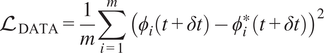(2.10) $$ {\mathrm{\mathcal{L}}}_{\mathrm{DATA}}=\frac{1}{m}\sum \limits_{i=1}^m{\left({\phi}_i\left(t+\delta t\right)-{\phi}_i^{\ast}\left(t+\delta t\right)\right)}^2 $$

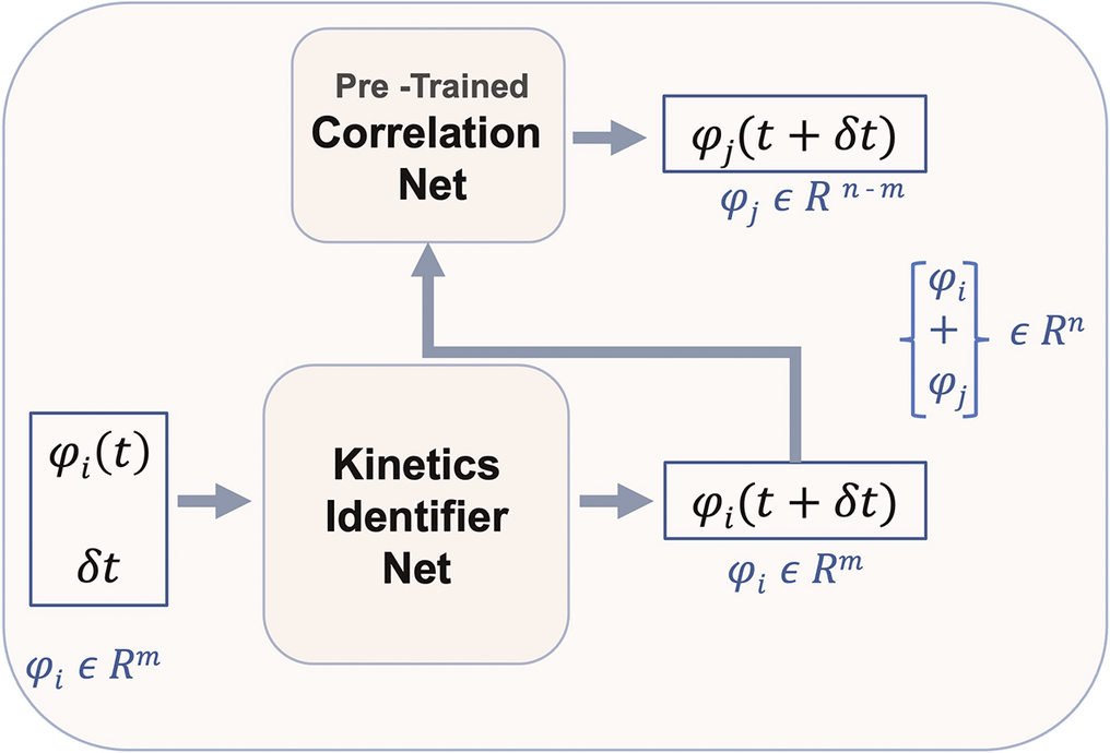
Figure 3. Full ANN coupling of React-DeepONet and Correlation Net.

The total loss becomes

(2.11) $$ \mathrm{\mathcal{L}}={W}_1{\mathrm{\mathcal{L}}}_{\mathrm{DATA}}+{W}_2{\mathrm{\mathcal{L}}}_{\mathrm{SUM}-\mathrm{MF}}+{W}_3{\mathrm{\mathcal{L}}}_{\mathrm{ELEM}} $$

where $ {W}_1 $ , $ {W}_2 $ , and $ {W}_3 $ are the weights for each loss term. Again, element and mass conservation as in Eq. (2.7) may be redundant. Therefore, enforcing element conservation loss alone is sufficient to establish mass and element conservation, and either weight, $ {W}_1 $ or $ {W}_2 $ , can be set to zero. Although, preferably, $ {W}_2 $ should be kept and $ {W}_1 $ can be set to zero. We will again investigate whether enforcing this redundancy in mass and element conservation can improve the training in the Results section.

Finally, we note that the solution vector in the network shown in Figure 3 is subjected to both a transformation and a normalization. The main exception is where we implement the loss function evaluation, where we need to transform the species mass fractions to their actual values to impose mass and element conservation. The transformation and scaling procedure is implemented as follows:

• • A fifth-order transformation is implemented on the species profiles and temperature to accommodate their strong variations. For example, for the $ k $ th species mass fraction, $ {Y}_k $ , this transformation is implemented as follows:

  (2.12) $$ {y}_k={Y}_k^{1/5} $$

• • In a second step, we normalize the transformed variables, $ {y}_k $ , to yield values in the range of −1 to 1 among all the training data by using the minimum and maximum values of each transformed quantity.

3. Results

This section presents validation results for our proposed framework to predict species profiles and reduce enforced mass and element conservation. As stated above, we demonstrate the framework using our React-DeepONet approach (Kumar and Echekki, 2024. The data is generated using 0D homogeneous chemistry simulations at constant atmospheric pressure for CH $ {}_4 $ oxidation. We have chosen to validate our approach using 0D data and without advective or diffusive transport typical of 3D reacting flow simulations to unambiguously establish element and mass conservation with the proposed framework. Although Mehl and Aubagnac-Karkar (2023) relied on a model that involves 0D stochastic particles with mixing, the enforcement of mass conservation is implemented on the reaction source operator only. A similar strategy was adopted by Readshaw et al. (2023), who used unsteady premixed flames but enforced mass conservation on the reaction source operator. It is equally important to note that the proposed framework can be extended to a broad range of chemical states (including states that result from reaction and transport) by using multiple React-DeepONets with mass/element conservation for different regions of the composition space of interest using clustering techniques.

The solution profiles for training purposes are generated using Cantera (Goodwin et al., 2022) with the GRI-Mech 3.0 (Smith et al., 1999) mechanism with 53 species and 325 reversible reactions. The solution vector consisting of species mass fractions and temperature is evolved in time for a total of 100 initial conditions of methane–air mixtures with 10 initial temperatures equally spaced from $ {T}_i $ = 1100 K to 1150 K and 10 equivalence ratios equally spaced from 0.8 to 1.2. Of these 100 profiles, 90 are used for training and 10 for testing. This data corresponds to outputs of the solution vector at increments of $ {10}^{-6} $ s from 0 to 8 ms.

Instead of the full thermo-chemical vector (54 scalars), the reduced set of eight representative species, including H₂, H₂O, CH₄, CO₂, CH₃OH, O₂, CO, and NO, and temperature are considered for the chemical kinetics learning through the React-DeepONet model. The list of representative species is chosen based on the two-step PCA process of Alqahtani and Echekki (2021). The method is designed to select species whose reactions contribute the most to all species in the chemical system. The list also includes all the major species involved during methane oxidation. The remaining 45 species in the GRI-Mech 3.0 are modeled as nonrepresentative species within the proposed framework. Their mass fractions are modeled using Correlation Net based on the input of the temperature and eight representative species listed above.

Other methods can be used to determine representative scalars. They include the use of DRGs (Lu and Law, 2005), the GPS algorithm of Gao et al. (2016), or the manifold-informed representative species selection method by Zdybał et al. (2023).

As discussed above, Correlation Net is pretrained with the physical constraints on the full dataset, where the representative and nonrepresentative species are inputs and outputs to the model, respectively. Then, utilizing the mapping from the pretrained Correlation Net, the React-DeepONet model is trained with the physical constraints of mass and elemental conservation.

Both Correlation Net and React-DeepONet are modeled and trained with the JAX framework (Frostig et al., 2018) on an NVIDIA RTX A5500 GPU with the Adamax optimizer (Kingma and Ba, 2014). The size of trainable parameters of Correlation Net is around 2000, and for React-DeepONet, it is around 200,000. Correlation Net and React-DeepONet are trained for 300,000 and 80,000 iterations, taking around 3.3 minutes and 10.5 minutes, respectively, of GPU time. The detail of architectures and training hyperparameters for both React-DeepONet and Correlation Net are listed in Table 1. As the table shows, much of the network complexity resides in the React-DeepONet network, while the reconstruction of the nonrepresentative species is implemented with only two hidden layers. However, the total training time is comparable. Moreover, the same activation function, Tanh, and the same loss function, MSE, are used in both networks.

Table 1. ML models and training hyperparameters

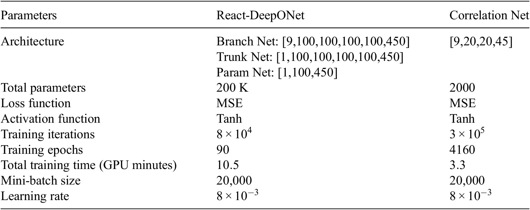
Note. The architecture of each network or subnetwork is indicated within square brackets, showing the number of neurons per layer.

The obtained input–output pairs from training initial conditions are further broken down in an 80/20 ratio to extract the validation dataset. Figure 4 shows the decay of data loss, the sum of mass fraction loss, and elemental conservation loss during the training of Correlation Net and React-DeepONet for training as well as the validation dataset. Different observations can be made related to the trends of the different loss terms. First, the validation loss decay is almost identical between training and validation losses, indicating that the model hyperparameters are well optimized. Second, the mass and element conservation losses exhibit the same trends in their rate of convergence and magnitude in the Correlation Net and the combined network losses. Note that the weights for these losses are assigned the same values. Therefore, as suggested above, the element and mass conservation losses are redundant, and enforcing mass and element conservation simultaneously is not needed. Therefore, we can eliminate considerations for the mass conservation losses in both the pretrained Correlation Net and the combined networks. Finally, by adding conservation losses (see Figure 4), the errors associated with these losses are significantly reduced relative to the data loss contributions.

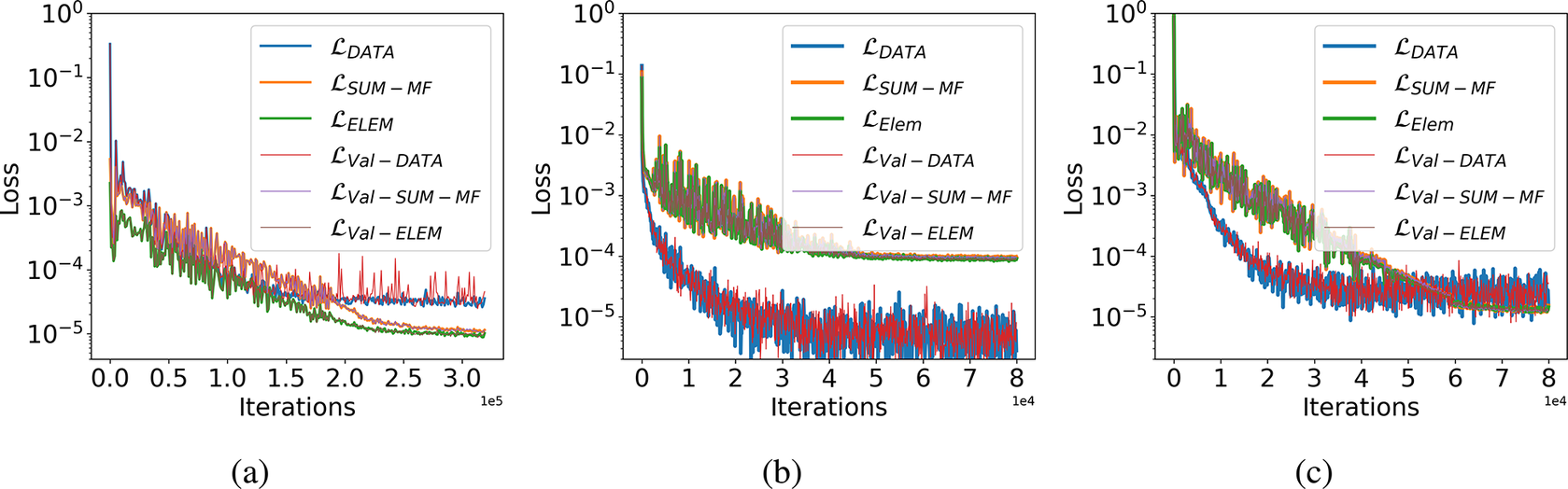
Figure 4. Loss decay for training and validation dataset. (a) Correlation Net training loss decay with physical constraints of species and elemental mass conservation. (b) React-DeepONet training loss decay without physical constraints. (c) React-DeepONet training loss decay with physical constraints.

In Figure 4a, the decay in the loss corresponding to the species and elemental mass conservation in the training of Correlation Net ensures that the trained model is physically more compliant. Figure 4b,c shows the React-DeepONet training loss with and without constraints of conservation laws, respectively. It is evident that, during the kinetics learning from React-DeepONet, losses corresponding to the conservation laws further decay by more than one order of magnitude when corresponding conservation constraints are imposed during the training. Figure 4 suggests that a range of values for the weights in Eq. (2.7) can be adapted to highlight a particular loss contribution. With equal weights, the dominant loss terms may correspond primarily to those of the solution mapping or the sum of the mass fractions constraints. In this study, we selected the following weights for individual losses in the total loss formulation: $ {W}_1 $ , $ {W}_2 $ and $ {W}_3 $ are 0.6, 0.2, and 0.2, respectively, for the training of both Correlation Net and React-DeepONet. We find that a range of values of these weights, within a factor of 2 or 3, yields similar outcomes in mapping solution vectors across time steps while enforcing mass conservation constraints.

3.1. Validation of Correlation Net

In this section, we first validate the standalone Correlation Net before its integration with React-DeepONet. In this validation study, we construct the Correlation Net model using the Cantera simulations on test data, where nonrepresentative species (the output of Correlation Net) are evaluated in terms of the representative species (the input of Correlation Net). The comparisons are carried out using the Cantera predictions for the nonrepresentative species. Individual temporal profiles of species are compared for one run condition, corresponding to an initial methane-air mixture at 1135 K and an equivalence ratio of 1.1. This condition is part of the testing data, not the training data. Similar trends are observed for other initial temperatures and mixture conditions. We will also present comparisons of the different test cases by integrating errors across the entire time evolution of individual profiles.

Figure 5 compares the temporal profiles of three nonrepresentative and minor species, OH, C₂H₄, and NH₃, mass fractions based on the Cantera solutions (solid lines) and their recovery using Correlation Net (symbols). Note that the solutions are normalized using minimum and maximum values to illustrate the results for the various species in one plot. The results show an initial methane–air mixture at 1135 K and an equivalence ratio of 1.1. They correspond to the case where mass and element conservation are integrated with the loss evaluations of Correlation Net. The comparison of the three nonrepresentative species shows an excellent agreement, indicating that Correlation Net provides an adequate prediction of nonrepresentative species. Similar results are obtained for other nonrepresentative species in the methane mechanism but are not shown here. More importantly, implementing mass and element conservation constraints significantly reduces the prediction errors of Correlation Net.

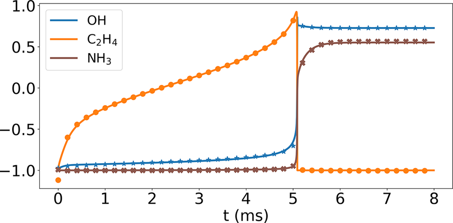
Figure 5. (Correlation Net) Reconstruction of three nonrepresentative species temporal profiles for $ {T}_i $ =1135 K and an equivalence ratio of 1.1.

Figure 6 shows comparisons of the temporal profiles of the NH₃ mass fraction from the Cantera solution (blue lines) and the Correlation Net predictions with (green lines) and without (red lines) mass and element conservation enforced. The figure also illustrates the errors in the predictions of the mass and element conservation with and without the mass/element conservation constraints. For mass conservation, the reported value corresponds to the sum of the mass fractions of the representative and nonrepresentative species, recovered by Correlation Net. With mass conservation, this sum should have a value of 1. For element conservation, the results are shown for the elemental mass fraction, which can be expressed for the element $ i $ as follows:

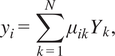(3.1) $$ {y}_i=\sum \limits_{k=1}^N{\mu}_{ik}{Y}_k, $$

where $ {y}_i $ is the elemental mass fraction for element $ i $ , $ {Y}_k $ is the mass fraction of the $ k $ the species, and $ {\mu}_{ik} $ is the mass fraction of element $ i $ in the $ k $ th species. This elemental mass fraction must remain constant for homogeneous chemistry since reactions do not alter elements. Moreover, the sum of all elemental mass fractions must also be 1.

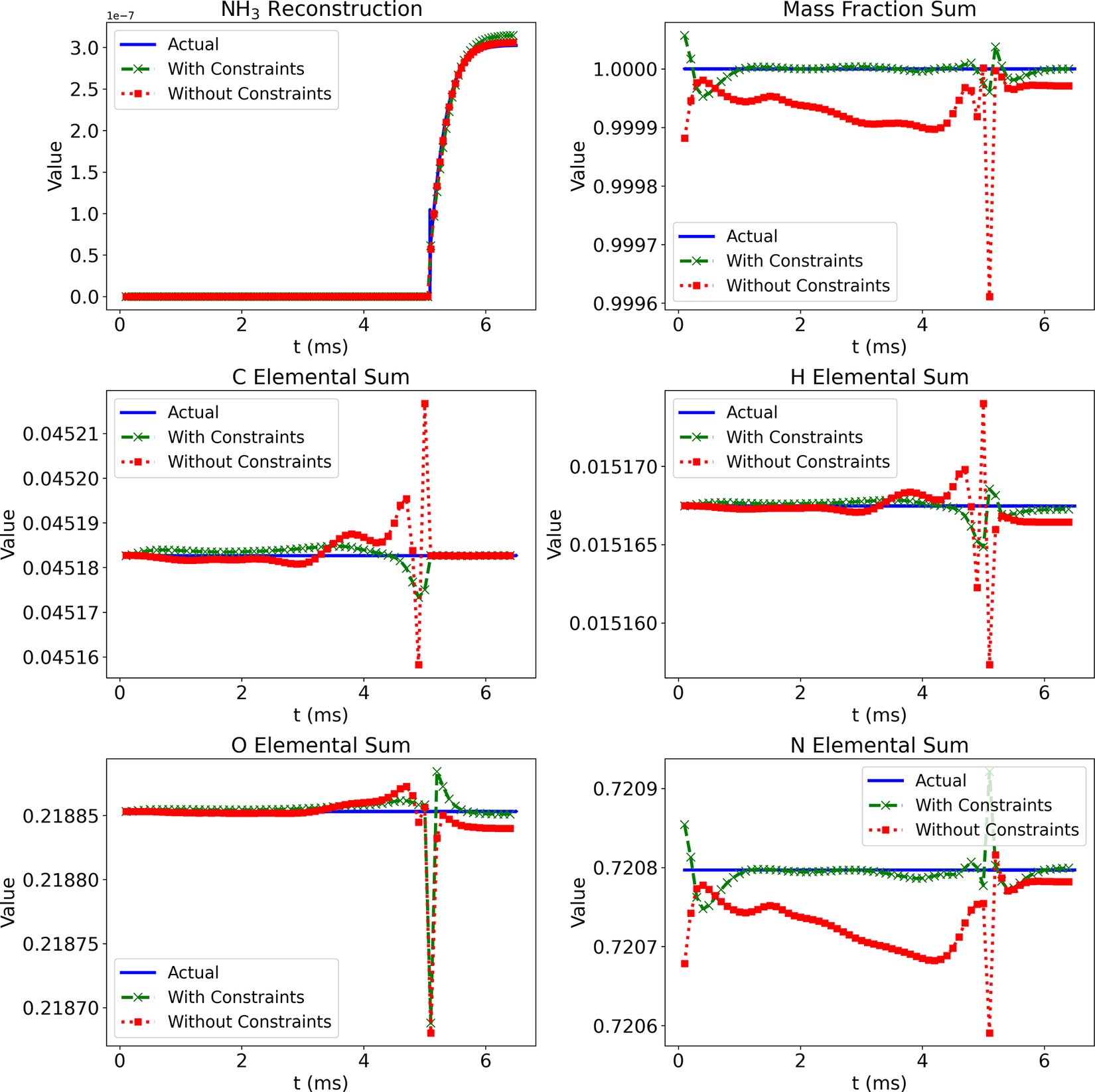
Figure 6. (Correlation Net) Prediction of NH $ {}_3 $ profiles and validation of mass and element conservation with and without physical constraints ( $ {T}_i $ = 1135 K and an equivalence ratio of 1.1).

The NH₃ mass fraction profiles for the Correlation Net with and without conservation constraints are indistinguishable. The difference between the two sets of predictions can only be seen when looking closely at the errors incurred for mass and element conservation. From the profiles, it is clear that imposing these errors is much lower when mass and element conservation are incorporated within the loss evaluations of Correlation Net.

As expected, the elemental mass fractions from the Cantera solution remain fixed for all elements considered. With Correlation Net, incorporating the mass and element conservation losses significantly reduces the deviation from the expected constant predictions. Yet, this deviation remains reasonably small whether conservation constraints are imposed or not.

So far, we have presented the above results based on one test case corresponding to a prescribed initial temperature and equivalence ratio. Figure 7 shows the mean absolute errors (MAEs) associated with mass and element conservation for the 10 test cases considered using Correlation Net with and without incorporating conservation losses. The MAEs are based on averages across different states along the integration trajectory for each solution using the original denormalized quantities. For mass conservation, the MAE is based on the deviation of the sum of representative and nonrepresentative species relative to 1. For element conservation, the MAE is based on the deviation of the elemental mass fraction from the constant value computed in Cantera for each element.

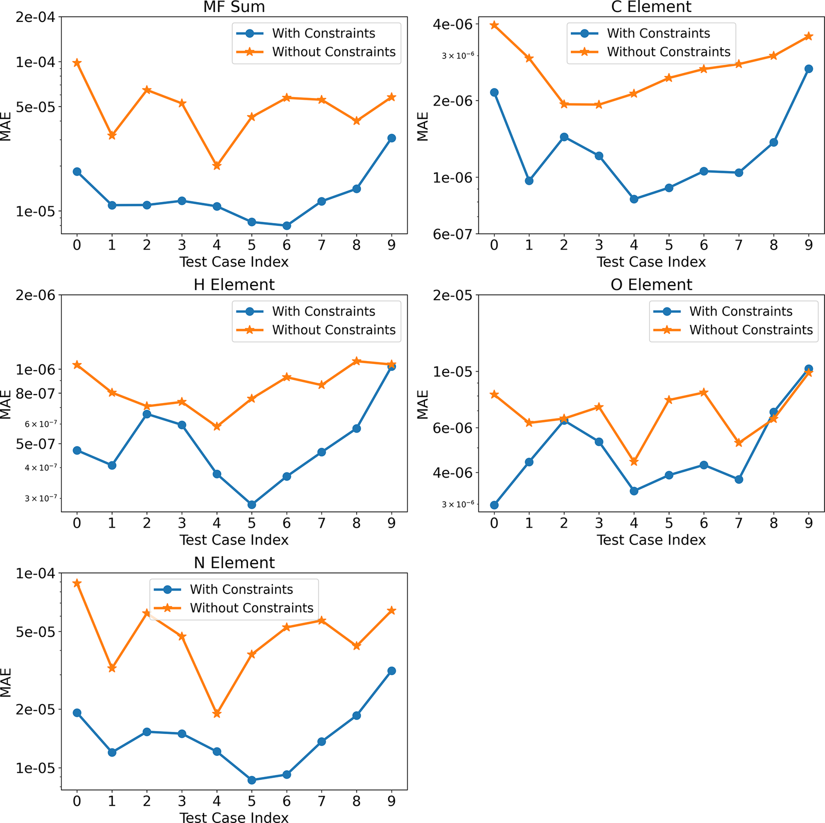
Figure 7. (Correlation Net) Time-averaged mean absolute errors for mass and element conservation with and without conservation constraints for all test cases.

The results clearly show that Correlation Net with and without the incorporation of losses can still result in errors that are less than 0.1% of the fixed values for the sum of mass fractions or elemental mass. As expected, incorporating mass and element conservation significantly reduces the error of recovering nonrepresentative species with Correlation Net. This reduction in error is approximately one order of magnitude for C, H, O, and N.

Figure 8 shows the MAE for species and temperature predictions for all test cases based on the training of Correlation Net and corresponding to the scenarios of implementing mass/element constraints or not implementing them. Recall that both scenarios are trained with an MSE loss formulation. The reconstruction MAE tends to be slightly higher with the implementation of the constraints, given the additional contributions to the loss function. Nonetheless, the predictions tend to be uniform across all test cases.

Figure 8. (Correlation Net) Time-averaged MAE for species and temperature predictions from Correlation Net with and without constraints for all the test cases.

Finally, it is important to note that the Correlation Net predictions of the species presented in Figure 5 are typical for all solution profiles within the range of the training data and for all species evaluated through Correlation Net. No discernable variations exist between OH, C₂H₄ and NH₃ predictions and those of other species in the mechanism. Therefore, the time-averaged MAE plots shown in Figure 8 represent the performance of the individual species reconstructed using Correlation Net.

3.2. A posteriori comparisons with COrrelation Net and React-DeepONet

Next, we present the results of the a posteriori predictions of Correlation Net with and without mass and element conservation with its integration of React-DeepONet. In contrast with the previous discussion, the a posteriori calculation of the species involves the evaluation of the evolution of the representative species in time and is implemented using React-DeepONet. The nonrepresentative species are again recovered using Correlation Net with an input corresponding to the predicted representative species.

Figures 9–11 illustrate the same results presented in Figures 5–7, respectively. As shown in Figure 9, the a posteriori results for combining Correlation Net and React-DeepONet can accurately reproduce profiles of nonrepresentative species. Similar to earlier observations, Figure 10 also shows that adding mass and element conservation in Correlation Net achieves its desired objectives. This is demonstrated in one case in Figure 10 in addition to 10 cases, as shown in Figure 11. We observe similar trends for the MAE error reduction for mass and element conservation as obtained using Correlation Net alone.

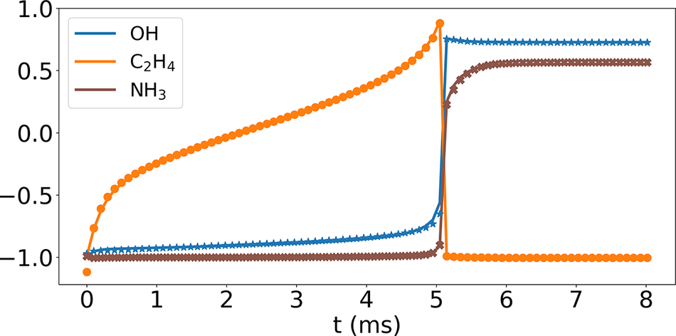
Figure 9. (Correlation Net + React-DeepONet) Reconstruction of three nonrepresentative species temporal profiles for $ {T}_i $ = 1135 K and an equivalence ratio of 1.1.

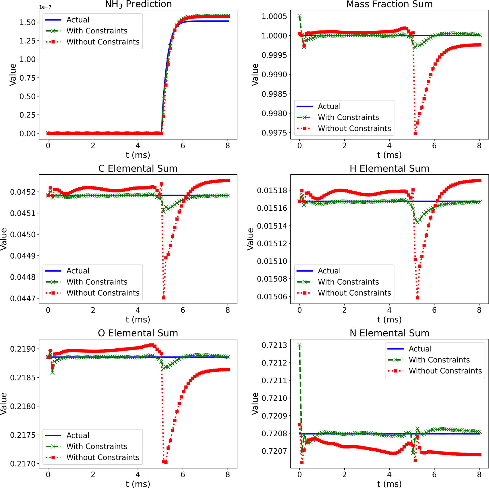
Figure 10. (Correlation Net + React-DeepONet) Prediction of NH $ {}_3 $ profiles and validation of mass and element conservation with and without physical constraints ( $ {T}_i $ = 1135 K an equivalence ratio of 1.1).

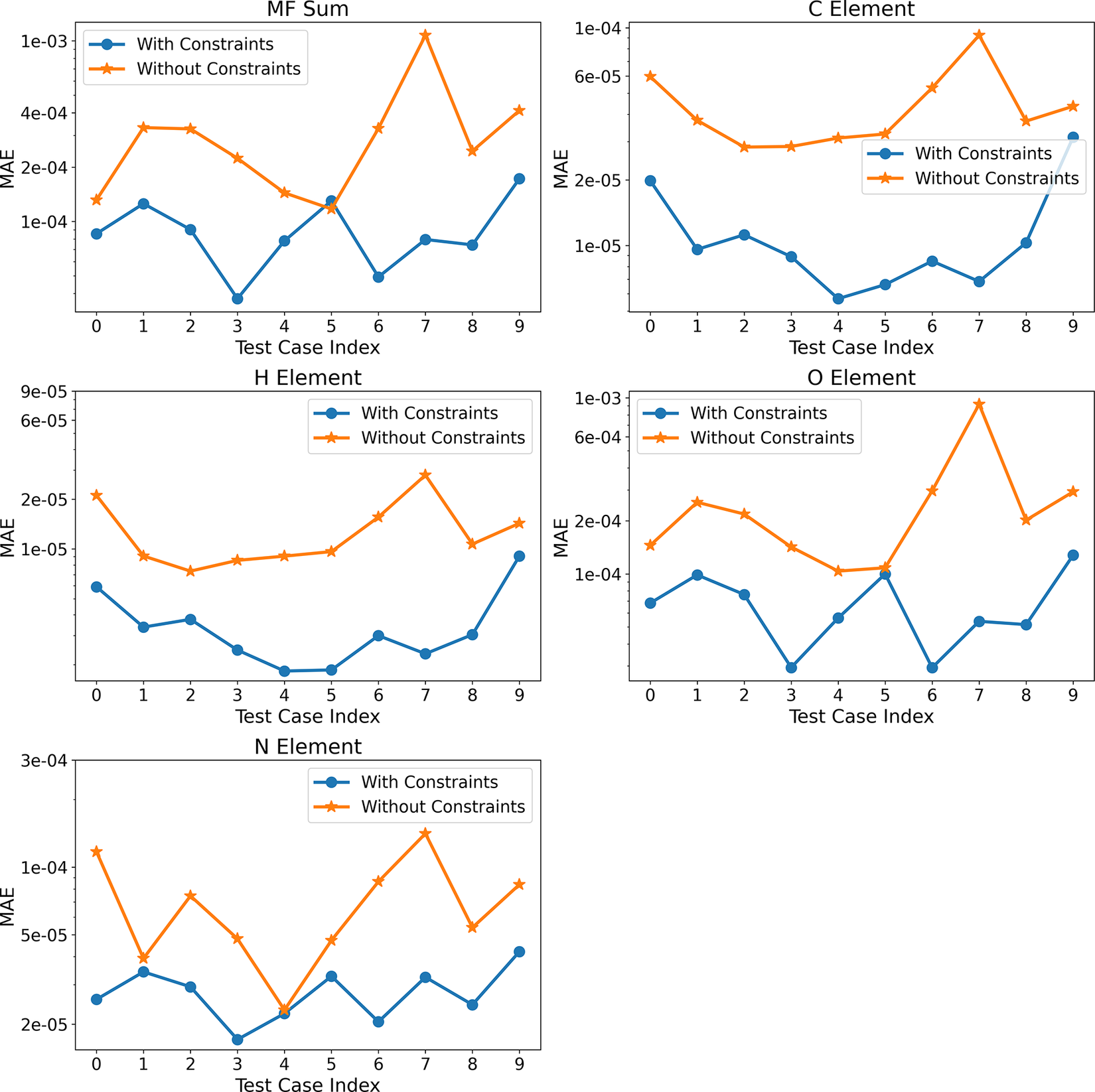
Figure 11. (Correlation Net + React-DeepONet) Time-averaged mean absolute errors for mass and element conservation with and without conservation constraints for all test cases.

Figure 12 shows the time-averaged MAE for species and temperature predictions from the entire network combining React-DeepONet and Correlation Net for all test cases considered for the two scenarios, where mass/element conservation is implemented or not. Again, both scenarios are trained with an MSE loss formulation. In contrast with the predictions based on Correlation Net alone, as shown in Figure 8, the MAE values can be higher or lower between the two scenarios. Yet, their magnitudes are again comparable and do not vary significantly among the different test cases.

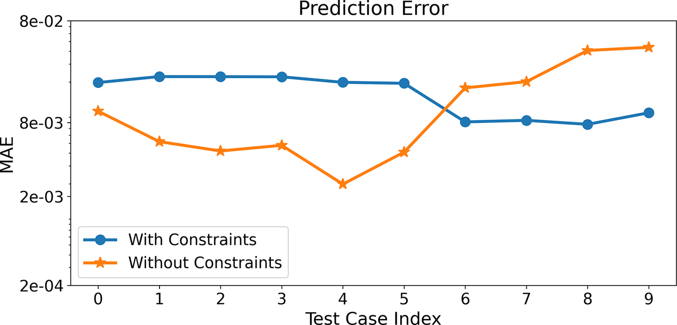
Figure 12. (Correlation Net + React-DeepONet)Time-averaged MAE for species and temperature predictions from React-DeepONet with and without constraints for all the test cases.

4. Conclusions

In this study, we propose and implement a physics-constrained model for mass and element conservation within a framework of chemistry integration and an approach to recover nonrepresentative species while advancing the solution of a subset of the chemical system. The implementation involves the coupling of the reduced-state framework with a Correlation Net to recover nonrepresentative species and constraints on mass and element conservation implemented on the overall network. The coupled framework significantly improves mass and element conservation and can predict (representative and nonrepresentative) species as a potentially reduced computational cost.

The principal advantage of the proposed approach is the potential implementation of the chemistry integration framework with element and mass conservation in reacting flow simulations. With a choice of a subset of the chemical species and mapping solutions across time increments, computational and memory savings can be achieved. The advantage of this framework for complex combustion fuels can be critical as the solution vector can be reduced from hundreds or thousands of transported species to a range from 10 to 20 representative species. The proposed scheme is also able to recover nonrepresentative species. With the use of Correlation Net, the nonrepresentative species can be used for postprocessing purposes in addition to the accurate evaluation of thermodynamic and transport properties during a simulation.