1 Introduction
Collaboration across organizational boundaries in engineered systems presents an important tradeoff during conceptual design. Distributed architectures where multiple actors cooperate for mutual benefit seek superior performance compared to independent architectures. Potential improvement may derive from increased flexibility (de Weck et al. Reference de Weck, de Neufville and Chaize2004), robustness (Brown and Eremenko Reference Brown and Eremenko2006), or efficiency (Oates Reference Oates, Auerbach and Shaviro2008). However, collaborative architectures also introduce new interdependencies between constituent systems which can lead to degraded performance or failure if not treated as a system of systems (Maier Reference Maier1998).
Understanding and reasoning about the tradeoff between risk and reward in collaborative system architectures remains a critical area of research. It underlies ongoing challenges in managing inter-agency collaboration in joint projects (National Research Council 2011) as well as new laws requiring public agencies such as the National Oceanic and Atmospheric Administration (NOAA) to consider purchasing data from commercial providers to supplement government missions (United States of America 2017). Improved methods to understand fundamental collaborative dynamics early in the conceptual design and architecture selection phase could help avoid costly coordination failures.
Risk fundamentally deals with the interaction between probability and consequence of alternative scenarios (Kaplan and Garrick Reference Kaplan and Garrick1981). In engineering design, decision-makers routinely employ risk analysis methods to help choose among alternative design concepts (Lough et al. Reference Lough, Stone and Tumer2009). Traditional perspectives on risk for engineered systems consider potential impacts of external factors such as natural disasters or attacks and internal factors such as component fatigue, failure, or error. However, collaborative systems exhibit an additional source of uncertainty attributed to coordination failures among interacting decision-makers. This strategic source of risk is not addressed by methods that view engineering design as a centralized decision-making process.
This paper transitions the analytical concept of risk dominance from equilibrium selection in game theory to engineering design to measure the relative risk of coordination failures in collaborative systems at a level suitable for conceptual trade studies. Risk dominance recognizes the fragility of joint decisions and seeks to balance potential rewards with downside risk of coordination failure. This paper contributes a method to formulate collective design problems as a strategic design game and measure risk dominance. This paper provides a rigorous treatment of risk dominance in engineering design with two or more asymmetric players and overcomes barriers in transitioning fundamental theory to application. Results of this work can be used to inform conceptual phase architecture trades between collaborative and independent alternatives.
The remainder of this paper is organized as follows. Section 2 reviews applications of economics and game theory in engineering design literature and introduces the stag hunt game as the intellectual foundation for collaborative systems. Section 3 proposes a method to formulate collective systems design as strategic design games to assess strategic risk dominance with two or more players. Section 4 introduces an application case to show how risk dominance can identify and mitigate potential sources of coordination failure in an asymmetric three-player design scenario. Finally, a conclusion summarizes contributions, assumptions and limitations, and future work.
2 Background
2.1 Utility-based methods in systems design
This section builds on a line of literature dating to early works by Simon (Reference Simon1959) that develop and apply economic methods for decision-making to a broad class of problems including engineering design. From this perspective, engineering design selects the alternative concept with highest value (under expectation) measured using von Neumann–Morgenstern utility (Hazelrigg Reference Hazelrigg1998). This approach is normative to organize and process individual preferences to support decision-making rather than descriptive to explain why certain decisions were made (Thurston Reference Thurston2001). Multi-criteria decision analysis methods including multi-attribute utility theory, analytic hierarchy process, and others help to formulate decisions for complex problems (Velasquez and Hester Reference Velasquez and Hester2013).
Applying multi-criteria decision analysis to collective systems design problems characteristically transforms each participating actor’s preferences into objective functions, defining an optimization problem. Although arguments have been made both against and in favor of this approach, most engineering design literature does not address essential uncertainty resulting from interactive effects between independent decision-makers. For instance, comparing engineering design to a social choice problem and grounded on Arrow’s (Reference Arrow1963) Impossibility Theorem, Hazelrigg (Reference Hazelrigg1997) argues that an optimal solution can only be reached if all actors share the same utility function; otherwise, any attempt to maximize aggregated individual gains is bound to result in ‘irrational’ outcomes – assuming that a ‘rational’ design maximizes every designer’s expected utility. In contrast, Scott and Antonsson (Reference Scott and Antonsson1999) state the purpose of engineering problems is to meet requirements, not individuals’ wishes, and thus engineering design exists on a continuum between single- and multi-actor problems and any disparity between system requirements and decision-makers’ preferences should be made explicit. However, in a collective systems design process with independent decision authority, actors strategically retain information and, as a result, do not have full knowledge about each other’s preferences.
Recent design research emphasizes value-centric or value-driven design methods building on rational decision-making theory to maximize system value rather than meeting requirements at minimum cost (Collopy and Hollingsworth Reference Collopy and Hollingsworth2011). A related class of methods for tradespace exploration enumerate a design space and evaluate one or more design attributes to visualize a set of alternatives (Ross et al. Reference Ross, Hastings, Warmkessel and Diller2004). These approaches generally treat risk as uncertainty or variation in value which can be analyzed with Monte Carlo sampling of a stochastic value function (Walton and Hastings Reference Walton and Hastings2004; O’Neill et al. Reference O’Neill, Yue, Nag, Grogan and de Weck2010; Daniels and Paté-Cornell Reference Daniels and Paté-Cornell2017). When applied to collective systems design, tradespace exploration results in computationally intense calculations due to combinatorial factors of a large design space coupled with interactive effects between actors. More importantly, this type of risk should not be considered as an explicit attribute to be traded during concept evaluation but only as uncertainty on other attributes (Abbas and Cadenbach Reference Abbas and Cadenbach2018). More focused analysis of strategic dynamics is necessary to understand risk in collaborative systems.
2.2 Game-theoretic methods in systems design
In an attempt to reconcile multi-criteria decision analysis methods and limitations imposed from social choice applied to engineering design, Franssen and Bucciarelli (Reference Franssen and Bucciarelli2004) demonstrate how a game-theoretic approach to collective systems design can help designers reach satisfactory outcomes without disregarding the implications of conflicting actors’ preferences. Game theory analyzes strategic decision-making among multiple interacting actors or players. In the context of engineering design, the players are the design actors – cognizant individuals, computational agents, design organizations, or indirect stakeholders with undefined strategic interests (usually modeled as players from ‘nature’). Individual utility functions, typically referred to as payoff functions, describe the players’ preferences over the possible outcomes resulting from their actions. Each player also has a set of complete contingent plans or sequences of actions, i.e. strategies, from which to choose to maximize their expected gains depending on how much information they have about the other players’ actions.
Game-theoretical approaches to engineering design frequently do not provide enough details about what aspects of the problem equate to ‘strategies’ and what other elements constitute the strategic setting of collective action or ‘game’ to be studied. An existing body of work applies game theory to engineering design by equating design alternatives to strategy spaces (Vincent Reference Vincent1983; Lewis and Mistree Reference Lewis and Mistree1997; Briceño Reference Briceño2008; Wernz and Deshmukh Reference Wernz and Deshmukh2010). In these works, the strategy set is composed of continuous functions linked to the functional attributes of the system and game-theoretical methods inform design decision-making at a low level of abstraction. Normative methods evaluate and select design decisions based on idealistic scenarios of cooperative or non-cooperative strategic equilibria (Papageorgiou et al. Reference Papageorgiou, Eres and Scanlan2016).
The majority of contributions to engineering design literature grounded in game-theoretic methods search for stable design sets under strong assumptions of rationality – namely Nash equilibria – as solutions to the multi-actor design problem. To improve outcomes designated by Nash equilibria, some works develop methods to further explore the strategy space beyond rational reaction strategy sets (Gurnani and Lewis Reference Gurnani and Lewis2008; Herrmann Reference Herrmann2010). Other works explore subgame perfect equilibria as solution concepts to game-theoretical models of engineering design (Bhatia et al. Reference Bhatia, Kannan and Bloebaum2016; Kang et al. Reference Kang, Ren, Feinberg and Papalambros2016). Finding equilibria is computationally intense and sensitive to the strategy space definition, thus the number of design alternatives to be assessed should be kept at a minimum to allow for the best use of classical game-theoretical methods. Moreover, the existence of more than one equilibrium still leaves selection of a ‘best’ option in the air and rekindles the debate about what an optimal solution means from an rational/objective perspective.
2.3 Stag hunt game and risk dominance
In contrast to existing works applying game theory to engineering design which conflate design and strategy decisions for general problems, this paper adopts a simple strategic context to evaluate dynamics for a specific class of problems related to collective systems design. Analysis of risk dominance, a concept from equilibrium selection literature, provides insights about the relationships between interacting design actors and the relative stability of collaborative systems.
The stag hunt is a canonical game theory problem that models fundamental challenges in collective decision-making (Skryms Reference Skryms2004). It follows the narrative of two hunters deciding between two alternatives to either hunt stag or hare. A stag hunt provides a desirable reward but requires joint participation of both hunters (i.e. a single stag hunter goes home hungry). A hare hunt yields a modest reward and can either be performed alone or jointly. Depending on the particular game, an independent hare hunt may be more or less rewarding than a joint hare hunt; however, both cases must be preferred to a failed stag hunt and less desirable than a successful stag hunt.
Table 1. Stag hunt game with
![]() $u_{i}=\frac{2}{3}$
$u_{i}=\frac{2}{3}$

Table 1 shows a normal form payoff matrix for an example symmetric two-player stag hunt game with payoffs of 2 for a joint hare hunt, 3 for an individual hare hunt, 4 for a successful stag hunt, and 0 for a failed stag hunt. Rather than absolute wealth or resource quantities (e.g. amount of food), this paper treats payoff values as von Neumann–Morgenstern utilities that already account for behavioral factors such as loss aversion and diminishing sensitivity within each strategic context (Arrow Reference Arrow1971; Tversky and Kahneman Reference Tversky and Kahneman1992).
The strategy space
![]() ${\mathcal{S}}_{i}=\{\unicode[STIX]{x1D719}_{i},\unicode[STIX]{x1D713}_{i}\}$
denotes the hare and stag strategies, respectively, for player
${\mathcal{S}}_{i}=\{\unicode[STIX]{x1D719}_{i},\unicode[STIX]{x1D713}_{i}\}$
denotes the hare and stag strategies, respectively, for player
![]() $i$
. Inspection of selected strategy sets for two players (
$i$
. Inspection of selected strategy sets for two players (
![]() $s_{1},s_{2}$
) shows both
$s_{1},s_{2}$
) shows both
![]() $\unicode[STIX]{x1D719}=(\unicode[STIX]{x1D719}_{1},\unicode[STIX]{x1D719}_{2})$
and
$\unicode[STIX]{x1D719}=(\unicode[STIX]{x1D719}_{1},\unicode[STIX]{x1D719}_{2})$
and
![]() $\unicode[STIX]{x1D713}=(\unicode[STIX]{x1D713}_{1},\unicode[STIX]{x1D713}_{2})$
are Nash equilibria because neither player has unilateral incentive to deviate away from these points. From an equilibrium perspective both stag and hare strategies are stable; however, there are clear differences in risk and reward.
$\unicode[STIX]{x1D713}=(\unicode[STIX]{x1D713}_{1},\unicode[STIX]{x1D713}_{2})$
are Nash equilibria because neither player has unilateral incentive to deviate away from these points. From an equilibrium perspective both stag and hare strategies are stable; however, there are clear differences in risk and reward.
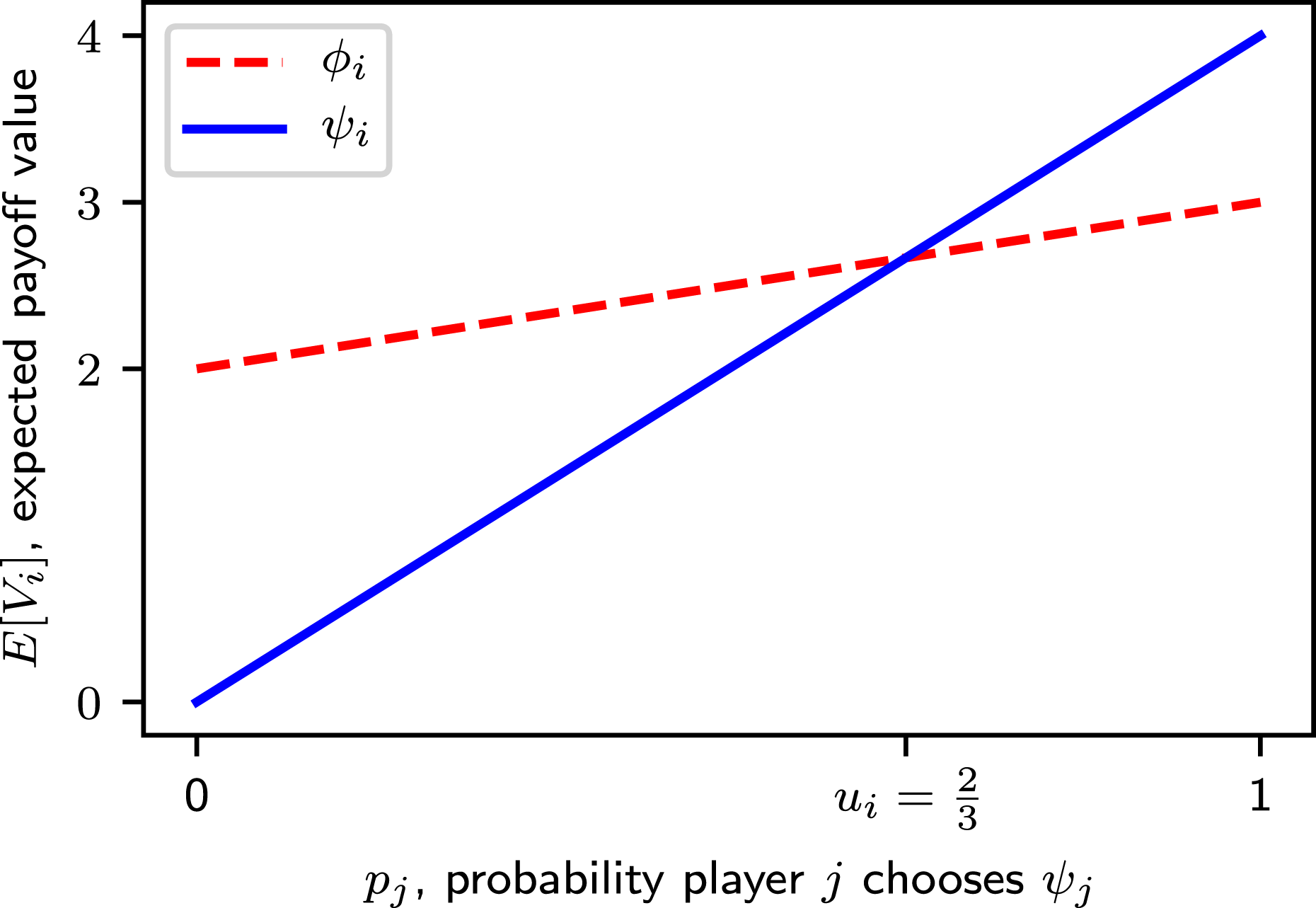
Figure 1. The expected value of strategies for player
![]() $i$
as a function of
$i$
as a function of
![]() $p_{j}$
, the probability that player
$p_{j}$
, the probability that player
![]() $j$
chooses
$j$
chooses
![]() $\unicode[STIX]{x1D713}_{j}$
for the example game in Table 1.
$\unicode[STIX]{x1D713}_{j}$
for the example game in Table 1.
Harsanyi and Selten (Reference Harsanyi and Selten1988) develop theory for equilibrium selection in bipolar games based on the concept of risk dominance. Similar to how some equilibria exhibit payoff dominance (i.e. the stag equilibrium
![]() $\unicode[STIX]{x1D713}$
yields higher payoffs), risk dominance is a desirable feature that captures resistance to losses.
$\unicode[STIX]{x1D713}$
yields higher payoffs), risk dominance is a desirable feature that captures resistance to losses.
In specific games such as the stag hunt with two strategies and two Nash equilibria (bipolar games), further analysis compares alternative strategies from a rational (expected value maximization) perspective. Figure 1 visualizes the expected value for player
![]() $i$
as a function of the probability that player
$i$
as a function of the probability that player
![]() $j$
chooses strategy
$j$
chooses strategy
![]() $\unicode[STIX]{x1D713}_{j}$
(i.e.
$\unicode[STIX]{x1D713}_{j}$
(i.e.
![]() $p_{j}=Pr\{s_{j}=\unicode[STIX]{x1D713}_{j}\}$
). For low values of
$p_{j}=Pr\{s_{j}=\unicode[STIX]{x1D713}_{j}\}$
). For low values of
![]() $p_{j}$
the hare strategy
$p_{j}$
the hare strategy
![]() $\unicode[STIX]{x1D719}_{i}$
provides the highest expected value. Similarly, for high values of
$\unicode[STIX]{x1D719}_{i}$
provides the highest expected value. Similarly, for high values of
![]() $p_{j}$
the stag strategy
$p_{j}$
the stag strategy
![]() $\unicode[STIX]{x1D713}_{i}$
provides the highest expected value. However, the two lines intersect at a point
$\unicode[STIX]{x1D713}_{i}$
provides the highest expected value. However, the two lines intersect at a point
![]() $0<u_{i}<1$
which measures the minimum probability of player
$0<u_{i}<1$
which measures the minimum probability of player
![]() $j$
choosing strategy
$j$
choosing strategy
![]() $\unicode[STIX]{x1D713}_{j}$
for it to be rational for player
$\unicode[STIX]{x1D713}_{j}$
for it to be rational for player
![]() $i$
to choose strategy
$i$
to choose strategy
![]() $\unicode[STIX]{x1D713}_{i}$
.
$\unicode[STIX]{x1D713}_{i}$
.
A closed-form expression in Eq. (1) computes
![]() $u_{i}$
for any two-player bipolar game for a given payoff function
$u_{i}$
for any two-player bipolar game for a given payoff function
![]() $V$
.
$V$
.
For the example in Table 1,
![]() $u_{1}=u_{2}=2/3$
. In other words, the expected value-maximizing decision for either player is to choose a stag hunt if and only if they estimate a better than two-in-three chance that their partner chooses a stag hunt.
$u_{1}=u_{2}=2/3$
. In other words, the expected value-maximizing decision for either player is to choose a stag hunt if and only if they estimate a better than two-in-three chance that their partner chooses a stag hunt.
Variations on the stag hunt game produce different values of
![]() $u_{i}$
. For example, Table 2 shows an alternative game for a scenario with a ‘trophy’ stag which increases the upside payoff from 4 to 11, lowering the threshold for economic collaboration to
$u_{i}$
. For example, Table 2 shows an alternative game for a scenario with a ‘trophy’ stag which increases the upside payoff from 4 to 11, lowering the threshold for economic collaboration to
![]() $u_{i}=0.2$
. Alternatively, Table 3 shows a scenario with an ‘injury’ incurred from a solitary stag hunt which decreases the downside payoff from 0 to
$u_{i}=0.2$
. Alternatively, Table 3 shows a scenario with an ‘injury’ incurred from a solitary stag hunt which decreases the downside payoff from 0 to
![]() $-2$
, raising the threshold for economic collaboration to
$-2$
, raising the threshold for economic collaboration to
![]() $u_{i}=0.8$
. These scenarios show that the structure of the payoff function influences perception of collaboration and is central to the concept of risk dominance.
$u_{i}=0.8$
. These scenarios show that the structure of the payoff function influences perception of collaboration and is central to the concept of risk dominance.
Table 2. Stag hunt game with
![]() $u_{i}=0.2$
$u_{i}=0.2$

Table 3. Stag hunt game with
![]() $u_{i}=0.8$
$u_{i}=0.8$

In the literature,
![]() $u_{i}$
is called the normalized deviation loss because its mathematical expression resembles a loss associated with deviating away from the equilibrium
$u_{i}$
is called the normalized deviation loss because its mathematical expression resembles a loss associated with deviating away from the equilibrium
![]() $\unicode[STIX]{x1D719}$
in the numerator normalized by the total losses associated with deviating away both equilibria in the denominator. Counter-intuitively, large deviation losses insulate a decision. The example in Table 2 shows the deviation loss from 11 to 3 promotes the stag strategy while the example in Table 3 shows the large deviation loss from 2 to
$\unicode[STIX]{x1D719}$
in the numerator normalized by the total losses associated with deviating away both equilibria in the denominator. Counter-intuitively, large deviation losses insulate a decision. The example in Table 2 shows the deviation loss from 11 to 3 promotes the stag strategy while the example in Table 3 shows the large deviation loss from 2 to
![]() $-2$
promotes the hare strategy.
$-2$
promotes the hare strategy.
Selten (Reference Selten1995) proposes a quantitative metric to measure risk dominance for bipolar games with linear incentives called the weighted average log measure (WALM) of risk dominance (see Appendix A for details). Linear incentives assume each player’s payoff can be expressed as a linear combination of whether other players participate in the collective strategy and is further addressed in Appendix B. Equation (2) defines the WALM of risk dominance for an
![]() $n$
-player game, where
$n$
-player game, where
![]() $u_{i}$
are normalized deviation losses and
$u_{i}$
are normalized deviation losses and
![]() $w_{i}$
are influence weights based on an influence matrix
$w_{i}$
are influence weights based on an influence matrix
![]() $A$
which measures player interdependence (Selten Reference Selten1995).
$A$
which measures player interdependence (Selten Reference Selten1995).
This expression maps bipolar games to a real-number scale that measures the risk dominance of the collective strategy
![]() $\unicode[STIX]{x1D713}$
relative to the independent strategy
$\unicode[STIX]{x1D713}$
relative to the independent strategy
![]() $\unicode[STIX]{x1D719}$
. For the objective case with no knowledge of other players’ actions (equivalent to
$\unicode[STIX]{x1D719}$
. For the objective case with no knowledge of other players’ actions (equivalent to
![]() $p_{j}=0.5$
),
$p_{j}=0.5$
),
![]() $R>0$
indicates
$R>0$
indicates
![]() $\unicode[STIX]{x1D719}$
is risk dominant while
$\unicode[STIX]{x1D719}$
is risk dominant while
![]() $R<0$
indicates
$R<0$
indicates
![]() $\unicode[STIX]{x1D713}$
is risk dominant. In all other cases with partial information leading to a probability distribution
$\unicode[STIX]{x1D713}$
is risk dominant. In all other cases with partial information leading to a probability distribution
![]() $f(p_{j})$
,
$f(p_{j})$
,
![]() $R$
provides a relative measure of risk dominance.
$R$
provides a relative measure of risk dominance.
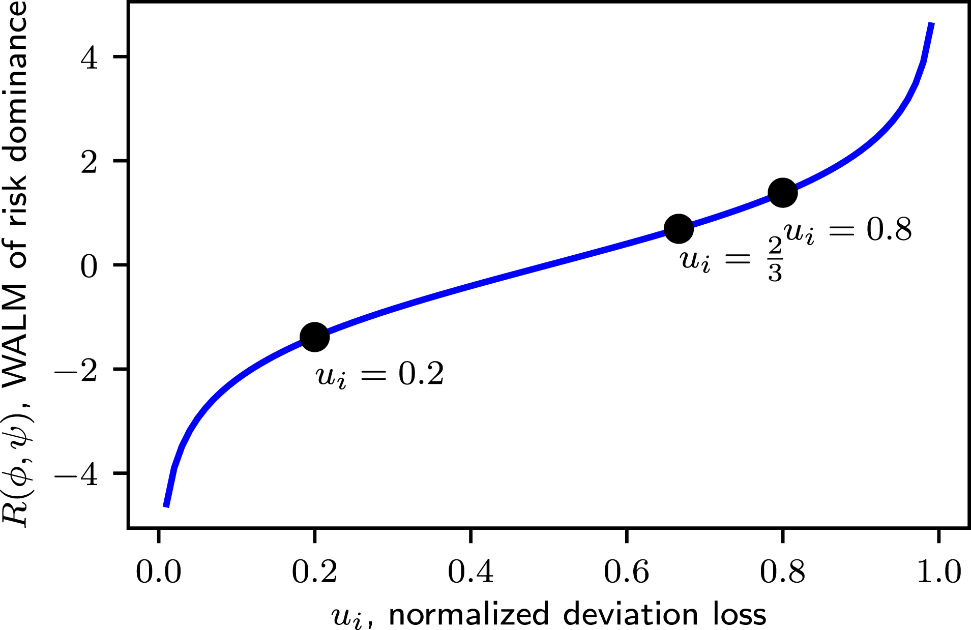
Figure 2. WALM of risk dominance is the logit function of the normalized deviation loss
![]() $u_{i}$
for symmetric games with
$u_{i}$
for symmetric games with
![]() $n=2$
players.
$n=2$
players.
WALM risk dominance can be simplified for games with
![]() $n=2$
players because weights are defined as
$n=2$
players because weights are defined as
![]() $w_{1}=w_{2}=1/2$
. Furthermore, payoff symmetry with
$w_{1}=w_{2}=1/2$
. Furthermore, payoff symmetry with
![]() $u_{1}=u_{2}=u_{i}$
further reduces the expression to Eq. (3) which is simply the logit function of
$u_{1}=u_{2}=u_{i}$
further reduces the expression to Eq. (3) which is simply the logit function of
![]() $u_{i}$
visualized in Figure 2.
$u_{i}$
visualized in Figure 2.
The stag hunt games in Tables 1–3 have
![]() $R_{1}=\ln 2\approx 0.69$
,
$R_{1}=\ln 2\approx 0.69$
,
![]() $R_{2}=\ln 0.25\approx -1.39$
, and
$R_{2}=\ln 0.25\approx -1.39$
, and
![]() $R_{3}=\ln 4\approx 1.39$
. In Table 2,
$R_{3}=\ln 4\approx 1.39$
. In Table 2,
![]() $R_{2}<0$
indicates the collective strategy
$R_{2}<0$
indicates the collective strategy
![]() $\unicode[STIX]{x1D713}$
is risk dominant. In Table 1 and Table 3,
$\unicode[STIX]{x1D713}$
is risk dominant. In Table 1 and Table 3,
![]() $R_{3}>R_{1}>0$
indicates the independent strategy
$R_{3}>R_{1}>0$
indicates the independent strategy
![]() $\unicode[STIX]{x1D719}$
is risk dominant and more strongly so in Table 3 compared to Table 1. Risk dominance is normative for strategy selection in non-cooperative cases; however, in other cases it is only a relative measure of strategic dynamics across games.
$\unicode[STIX]{x1D719}$
is risk dominant and more strongly so in Table 3 compared to Table 1. Risk dominance is normative for strategy selection in non-cooperative cases; however, in other cases it is only a relative measure of strategic dynamics across games.
While direct analysis of individual incentives in Figure 1 provides an intuitive explanation of strategic dynamics in two-player bipolar games, the more general formulation for WALM of risk dominance detailed in Appendix A handles asymmetric games with
![]() $n\geqslant 2$
players where players may express different or conflicting normalized deviation losses and pairwise interactions.
$n\geqslant 2$
players where players may express different or conflicting normalized deviation losses and pairwise interactions.
3 Risk dominance for collaborative systems
This section develops a method to convert a collective system design problem into a strategic design game to formulate and measure risk dominance.
3.1 Strategic design games
Game theory is a strategic analysis method that works at a high level of abstraction. In the context of engineering design, strategic decision-making best corresponds to architecture selection in conceptual design rather than more detailed design decisions in preliminary design. This section defines the concept of a strategic design game as a multi-actor value model for engineering decision-making to permit strategic analysis (Grogan et al. Reference Grogan, Ho, Golkar and de Weck2018).
Table 4. Stag hunt design utilities

Table 5. Stag hunt game with
![]() $u_{i}=0.5$
$u_{i}=0.5$

A strategic design game distinguishes between two levels of decisions: strategy decisions
![]() $s_{i}\in {\mathcal{S}}_{i}$
govern collective behavior among players and design decisions
$s_{i}\in {\mathcal{S}}_{i}$
govern collective behavior among players and design decisions
![]() $d_{i}\in {\mathcal{D}}_{i}$
specify system configurations. A corresponding multi-actor value function
$d_{i}\in {\mathcal{D}}_{i}$
specify system configurations. A corresponding multi-actor value function
![]() $[V_{i}^{s_{1},\ldots ,s_{n}}(d_{1},\ldots ,d_{n})]$
for
$[V_{i}^{s_{1},\ldots ,s_{n}}(d_{1},\ldots ,d_{n})]$
for
![]() $n$
players in Eq. (4) maps design and strategy decisions to values (utilities) for each player.
$n$
players in Eq. (4) maps design and strategy decisions to values (utilities) for each player.
While the design spaces
![]() ${\mathcal{D}}_{i}$
may be large or unbounded and unique to each player, the strategy space
${\mathcal{D}}_{i}$
may be large or unbounded and unique to each player, the strategy space
![]() ${\mathcal{S}}_{i}=\{\unicode[STIX]{x1D719}_{i},\unicode[STIX]{x1D713}_{i}\}$
is limited to two options: choosing between independent (
${\mathcal{S}}_{i}=\{\unicode[STIX]{x1D719}_{i},\unicode[STIX]{x1D713}_{i}\}$
is limited to two options: choosing between independent (
![]() $\unicode[STIX]{x1D719}_{i}$
) or collective (
$\unicode[STIX]{x1D719}_{i}$
) or collective (
![]() $\unicode[STIX]{x1D713}_{i}$
) action. Within each strategy space, design decisions are evaluated based on the context of the governing strategy.
$\unicode[STIX]{x1D713}_{i}$
) action. Within each strategy space, design decisions are evaluated based on the context of the governing strategy.
To illustrate this concept, reconsider the stag hunt game from Table 1 with design variables to choose the hunting weapon from the symmetric design space
![]() ${\mathcal{D}}=\{\text{Atlatl},\text{Bow},\text{Club},\text{Dog}\}$
. A multi-actor value model in Table 4 evaluates each design alternative in possible strategic contexts. Within fixed equilibrium contexts the best hare-hunting design is
${\mathcal{D}}=\{\text{Atlatl},\text{Bow},\text{Club},\text{Dog}\}$
. A multi-actor value model in Table 4 evaluates each design alternative in possible strategic contexts. Within fixed equilibrium contexts the best hare-hunting design is
![]() $\text{Dog}$
with utility 2 and the best stag-hunting design is
$\text{Dog}$
with utility 2 and the best stag-hunting design is
![]() $\text{Atlatl}$
with utility 4. However, as previously investigated in Table 1, this combination requires a probability greater than
$\text{Atlatl}$
with utility 4. However, as previously investigated in Table 1, this combination requires a probability greater than
![]() $u_{i}=2/3$
to pursue a stag hunt. In cases with unreliable partners, the stag-hunting design
$u_{i}=2/3$
to pursue a stag hunt. In cases with unreliable partners, the stag-hunting design
![]() $\text{Bow}$
in Table 5 may be more desirable because it only requires a probability greater than
$\text{Bow}$
in Table 5 may be more desirable because it only requires a probability greater than
![]() $u_{i}=0.5$
to pursue a stag hunt, although it only provides utility 3.5 if successful.
$u_{i}=0.5$
to pursue a stag hunt, although it only provides utility 3.5 if successful.
Applied to engineering design, the independent strategy
![]() $\unicode[STIX]{x1D719}_{i}$
corresponds to systems designed and operated with few external dependencies. The collective strategy
$\unicode[STIX]{x1D719}_{i}$
corresponds to systems designed and operated with few external dependencies. The collective strategy
![]() $\unicode[STIX]{x1D713}_{i}$
represents potential performance gains from collaborative systems having numerous interdependencies which operate at risk of degraded performance due to coordination failures. The resulting strategic design game resembles a binary game with zero, one, or two pure strategy Nash equilibria. Games with zero equilibria have no stable strategy sets, limiting the use of normative analysis. Games with one equilibrium exhibit a dominant strategy and do not benefit from further analysis. Therefore, only cases with two equilibria (i.e. bipolar games) benefit from and are valid to measure risk dominance.
$\unicode[STIX]{x1D713}_{i}$
represents potential performance gains from collaborative systems having numerous interdependencies which operate at risk of degraded performance due to coordination failures. The resulting strategic design game resembles a binary game with zero, one, or two pure strategy Nash equilibria. Games with zero equilibria have no stable strategy sets, limiting the use of normative analysis. Games with one equilibrium exhibit a dominant strategy and do not benefit from further analysis. Therefore, only cases with two equilibria (i.e. bipolar games) benefit from and are valid to measure risk dominance.
More detailed analysis of a strategic design game benefits from two simplifying assumptions in Eq. (5) and shown in Table 6 for a normal form strategic design game with
![]() $n=3$
players.
$n=3$
players.
 $$\begin{eqnarray}V_{i}^{s_{1},\ldots ,s_{n}}(d_{1},\ldots ,d_{n})=\left\{\begin{array}{@{}ll@{}}V_{i}^{\unicode[STIX]{x1D719}}(d_{i})\quad & \text{if}\,s_{i}=\unicode[STIX]{x1D719}_{i}\\ V_{i}^{\unicode[STIX]{x1D713}}(d_{k}:s_{k}=\unicode[STIX]{x1D713}_{k})\quad & \text{otherwise}.\end{array}\right.\end{eqnarray}$$
These assumptions limit interaction effects between participants inside and outside a collective strategy and are not strictly required for analysis but help to communicate the method and results using simplified notation.
The first simplification approximates the multi-actor value function by a single-actor value function
![]() $V_{i}^{\unicode[STIX]{x1D719}}$
when player
$V_{i}^{\unicode[STIX]{x1D719}}$
when player
![]() $i$
chooses an independent strategy
$i$
chooses an independent strategy
![]() $\unicode[STIX]{x1D719}_{i}$
. This assumes no strong interaction effects between independent players and others and allows local design optimization in Eq. (6).
$\unicode[STIX]{x1D719}_{i}$
. This assumes no strong interaction effects between independent players and others and allows local design optimization in Eq. (6).
The second simplification aggregates all candidate designs for players participating in a collective strategy
![]() $\unicode[STIX]{x1D713}$
including player
$\unicode[STIX]{x1D713}$
including player
![]() $i$
. For the special case where no other players select the collective strategy (i.e.
$i$
. For the special case where no other players select the collective strategy (i.e.
![]() $s_{j}=\unicode[STIX]{x1D719}_{j}\;\forall j\neq i$
), a single-actor value function
$s_{j}=\unicode[STIX]{x1D719}_{j}\;\forall j\neq i$
), a single-actor value function
![]() $V_{i}^{\unicode[STIX]{x1D713}}(d_{i})$
replaces the multi-actor one. This formulation emphasizes interaction effects among participants in a collective strategy but assumes no strong interaction effects with players outside.
$V_{i}^{\unicode[STIX]{x1D713}}(d_{i})$
replaces the multi-actor one. This formulation emphasizes interaction effects among participants in a collective strategy but assumes no strong interaction effects with players outside.
Table 6. Strategic design game for three players

3.2 Strategic risk dominance
This section uses the strategic design game concept to explain and measure risk dominance in collaborative systems design. Risk dominance is only meaningful in bipolar games which requires a specific ordering of value quantities such that
![]() $V_{i}^{\unicode[STIX]{x1D713}}(d_{1},\ldots ,d_{n})>{\mathcal{V}}_{i}^{\unicode[STIX]{x1D719}}>V_{i}^{\unicode[STIX]{x1D713}}(d_{i})\;\forall i$
. This is a reasonable requirement because it represents the cases of most interest where the collaborative system has a higher upside potential but also downside risk to an independent alternative.
$V_{i}^{\unicode[STIX]{x1D713}}(d_{1},\ldots ,d_{n})>{\mathcal{V}}_{i}^{\unicode[STIX]{x1D719}}>V_{i}^{\unicode[STIX]{x1D713}}(d_{i})\;\forall i$
. This is a reasonable requirement because it represents the cases of most interest where the collaborative system has a higher upside potential but also downside risk to an independent alternative.
As introduced in Section 2.3 and detailed in Appendix A, risk dominance first depends on normalized deviation losses. Equation (7) shows the normalized deviation loss for player
![]() $i$
by substituting the strategic design game notation into Eq. (1).
$i$
by substituting the strategic design game notation into Eq. (1).
 $$\begin{eqnarray}\displaystyle u_{i} & = & \displaystyle \frac{{\mathcal{V}}_{i}^{\unicode[STIX]{x1D719}}-V_{i}^{\unicode[STIX]{x1D713}}(d_{i})}{\left({\mathcal{V}}_{i}^{\unicode[STIX]{x1D719}}-V_{i}^{\unicode[STIX]{x1D713}}(d_{i})\right)+\left(V_{i}^{\unicode[STIX]{x1D713}}(d_{1},\ldots ,d_{n})-{\mathcal{V}}_{i}^{\unicode[STIX]{x1D719}}\right)}\nonumber\\ \displaystyle & = & \displaystyle \frac{{\mathcal{V}}_{i}^{\unicode[STIX]{x1D719}}-V_{i}^{\unicode[STIX]{x1D713}}(d_{i})}{V_{i}^{\unicode[STIX]{x1D713}}(d_{1},\ldots ,d_{n})-V_{i}^{\unicode[STIX]{x1D713}}(d_{i})}.\end{eqnarray}$$
The simplest form of strategic risk dominance assumes symmetric design spaces and utility functions for all players. Symmetry yields equal weighting factors
![]() $w_{i}$
, producing the risk dominance measure in Eq. (8) as a function of the collaborative design
$w_{i}$
, producing the risk dominance measure in Eq. (8) as a function of the collaborative design
![]() $d$
(note: all value subscripts dropped due to symmetry).
$d$
(note: all value subscripts dropped due to symmetry).
Symmetric risk dominance requires three function evaluations to quantify the upside value of a successful collective strategy
![]() $V^{\unicode[STIX]{x1D713}}(d,\ldots ,d)$
, downside value of a failed collective strategy
$V^{\unicode[STIX]{x1D713}}(d,\ldots ,d)$
, downside value of a failed collective strategy
![]() $V^{\unicode[STIX]{x1D713}}(d)$
, and the value of the independent alternative
$V^{\unicode[STIX]{x1D713}}(d)$
, and the value of the independent alternative
![]() ${\mathcal{V}}^{\unicode[STIX]{x1D719}}$
.
${\mathcal{V}}^{\unicode[STIX]{x1D719}}$
.
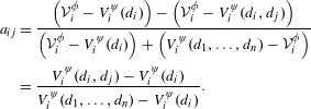
More general forms of strategic risk dominance assume asymmetric design spaces or utility functions. As detailed in Appendix A, influence elements
![]() $a_{ij}$
measure the dependence between players
$a_{ij}$
measure the dependence between players
![]() $i$
and
$i$
and
![]() $j$
. Equation (9) shows the influence elements
$j$
. Equation (9) shows the influence elements
![]() $a_{ij}$
between players
$a_{ij}$
between players
![]() $i$
and
$i$
and
![]() $j$
, assuming linear incentives, by substituting the notation for strategic design games into Eq. (27).
$j$
, assuming linear incentives, by substituting the notation for strategic design games into Eq. (27).
 $$\begin{eqnarray}\displaystyle a_{ij} & = & \displaystyle \frac{\left({\mathcal{V}}_{i}^{\unicode[STIX]{x1D719}}-V_{i}^{\unicode[STIX]{x1D713}}(d_{i})\right)-\left({\mathcal{V}}_{i}^{\unicode[STIX]{x1D719}}-V_{i}^{\unicode[STIX]{x1D713}}(d_{i},d_{j})\right)}{\left({\mathcal{V}}_{i}^{\unicode[STIX]{x1D719}}-V_{i}^{\unicode[STIX]{x1D713}}(d_{i})\right)+\left(V_{i}^{\unicode[STIX]{x1D713}}(d_{1},\ldots ,d_{n})-{\mathcal{V}}_{i}^{\unicode[STIX]{x1D719}}\right)}\nonumber\\ \displaystyle & = & \displaystyle \frac{V_{i}^{\unicode[STIX]{x1D713}}(d_{i},d_{j})-V_{i}^{\unicode[STIX]{x1D713}}(d_{i})}{V_{i}^{\unicode[STIX]{x1D713}}(d_{1},\ldots ,d_{n})-V_{i}^{\unicode[STIX]{x1D713}}(d_{i})}.\end{eqnarray}$$
Linear incentives enforce a constraint that all row sums total one, i.e.
![]() $\sum _{j\neq i}a_{ij}=1\,\forall \,i$
. In cases with nonlinear incentives for
$\sum _{j\neq i}a_{ij}=1\,\forall \,i$
. In cases with nonlinear incentives for
![]() $n=3$
players, as in Table 6, Eq. (10) expresses linearized influence elements
$n=3$
players, as in Table 6, Eq. (10) expresses linearized influence elements
![]() $\bar{a}_{ij}$
between players
$\bar{a}_{ij}$
between players
![]() $i$
and
$i$
and
![]() $j$
by substituting strategic design game notation into Eq. (2) (see Appendix B for details).
$j$
by substituting strategic design game notation into Eq. (2) (see Appendix B for details).
After computing elements of the influence matrix
![]() $A$
using linear incentives
$A$
using linear incentives
![]() $a_{ij}$
or the linear approximation
$a_{ij}$
or the linear approximation
![]() $\bar{a}_{ij}$
, subsequent analysis finds weighting factors
$\bar{a}_{ij}$
, subsequent analysis finds weighting factors
![]() $w_{i}$
to measure player importance. As detailed in Appendix A, weighting factors are the eigenvector corresponding to the unit eigenvalue of the influence matrix
$w_{i}$
to measure player importance. As detailed in Appendix A, weighting factors are the eigenvector corresponding to the unit eigenvalue of the influence matrix
![]() $A$
.
$A$
.
The risk dominance measure in Eq. (11) computes the WALM in Eq. (2) as a function of collaborative designs
![]() $(d_{1},\ldots ,d_{n})$
.
$(d_{1},\ldots ,d_{n})$
.
In general, asymmetric risk dominance requires
![]() $1+\sum _{k=1}^{n}\binom{n}{k}=2^{n}$
multi-actor value function evaluations to consider all possible combinations of players joining the collective strategy (required to compute
$1+\sum _{k=1}^{n}\binom{n}{k}=2^{n}$
multi-actor value function evaluations to consider all possible combinations of players joining the collective strategy (required to compute
![]() $\bar{a}_{ij}$
terms) plus the independent alternative. While not burdensome for small games, this combinatorial factor may limit the use of similar methods for large games with many decision-makers.
$\bar{a}_{ij}$
terms) plus the independent alternative. While not burdensome for small games, this combinatorial factor may limit the use of similar methods for large games with many decision-makers.
3.3 Assumptions and limitations
This work includes several key assumptions and limitations which must be discussed. First, measuring risk dominance assumes a strategic decision-making process structured as a bipolar game. The strategic design game is an abstraction of the design process where, in reality, lower-level design and higher-level strategy decisions are coupled and iterative. Results from this work thus provide a baseline result which must be considered in the context of a specific design problem. While a limiting constraint, bipolar games are interesting cases to study because they present a fundamental tradeoff between risk and reward.
Second, this work represents an analytical and rational/objective method to measure strategic risk dominance which is both a significant limitation and a significant strength. The strategic-level analysis only aims to maximize expected value – although utility functions to compute payoff values can incorporate risk attitudes. No subjective information is required to determine or assess the likelihood of other players’ actions nor are there any elements of cooperative game theory to enforce contracts or share or divide benefits (although
![]() $R$
is closely related to the Nash product and
$R$
is closely related to the Nash product and
![]() $\bar{a}_{ij}$
terms resemble Shapley value). If additional subjective information were available, a more thorough analysis leveraging Bayesian games could be performed, as pioneered by Harsanyi (Reference Harsanyi1967). In light of this limitation, relative values of the WALM risk dominance measure (e.g. during an architecture trade study) are more important than absolute values.
$\bar{a}_{ij}$
terms resemble Shapley value). If additional subjective information were available, a more thorough analysis leveraging Bayesian games could be performed, as pioneered by Harsanyi (Reference Harsanyi1967). In light of this limitation, relative values of the WALM risk dominance measure (e.g. during an architecture trade study) are more important than absolute values.
Third, the existing equilibrium selection theory imposes a few restrictions on the types of problems modeled. As discussed in Appendix A, it assumes linear incentives which are unlikely to hold in most engineering applications due to economies of scale; however, the linear approximation methods and error analysis introduced mitigate some of this concern. Developing utility functions to quantify payoff values while accommodating behavioral factors such as risk attitudes remains a practical challenge which is out of the scope of this paper.
Two other notational limitations can be relaxed for further analysis. The risk metric in Eq. (11) only assesses one set of collaborative architectures (
![]() $d_{1},\ldots ,d_{n}$
) under one collective strategy (
$d_{1},\ldots ,d_{n}$
) under one collective strategy (
![]() $\unicode[STIX]{x1D713}$
) relative to the independent baseline. However, as a real number,
$\unicode[STIX]{x1D713}$
) relative to the independent baseline. However, as a real number,
![]() $R$
can compare multiple design candidates relative to the same independent baseline (e.g.
$R$
can compare multiple design candidates relative to the same independent baseline (e.g.
![]() $R_{\unicode[STIX]{x1D713}}(d_{1},\ldots ,d_{n})$
vs.
$R_{\unicode[STIX]{x1D713}}(d_{1},\ldots ,d_{n})$
vs.
![]() $R_{\unicode[STIX]{x1D713}}(d_{1}^{\prime },\ldots ,d_{n}^{\prime })$
) to guide the design search process. Similarly,
$R_{\unicode[STIX]{x1D713}}(d_{1}^{\prime },\ldots ,d_{n}^{\prime })$
) to guide the design search process. Similarly,
![]() $R$
can compare multiple collective strategy candidates for a fixed set of federated alternatives (e.g.
$R$
can compare multiple collective strategy candidates for a fixed set of federated alternatives (e.g.
![]() $R_{\unicode[STIX]{x1D713}}(d_{1},\ldots ,d_{n})$
vs.
$R_{\unicode[STIX]{x1D713}}(d_{1},\ldots ,d_{n})$
vs.
![]() $R_{\unicode[STIX]{x1D713}^{\prime }}(d_{1},\ldots ,d_{n})$
) to guide the strategy formulation process.
$R_{\unicode[STIX]{x1D713}^{\prime }}(d_{1},\ldots ,d_{n})$
) to guide the strategy formulation process.
4 Illustrative application case
4.1 Multi-actor value model and design scenarios
This section develops an application case based on a stylized model of federated Earth-observing space systems paired with an existing simulation model. Orbital Federates Simulation – Python (OFSPY) (Grogan Reference Grogan2019) acts as a multi-actor value function by mapping design and strategy sets (inputs) to net present value earned by each player over a simulated system lifetime (outputs). The model includes stochastic features to capture operational uncertainty such that results must be sampled using Monte Carlo methods. While many model details are clearly fictional, the underlying model was developed to have structural and process isomorphic features to help understand strategic player behavior for space systems (Grogan and de Weck Reference Grogan and de Weck2015).
This application case only evaluates how to model collaborative design scenarios as a strategic design game and compute measures of risk dominance. The implementation details of the multi-actor value model are outside the scope of this paper; however, Appendix C provides more details for replication.
The design scenario considers
![]() $n=3$
players who operate space systems to collect and downlink data to satisfy demands and earn revenue. Figure 3 illustrates designs selected from a large combinatorial design space for a baseline (independent) strategic context and two federated alternatives. The independent case includes small standalone observing spacecraft for players 2 and 3 who specialize in synthetic aperture radar (SAR) and visual light (VIS) sensors, respectively. Player 1 does not participate in the baseline system. Federated designs consider an opportunistic data exchange policy with a fixed price for inter-satellite link (ISL) and space-to-ground (SGL) services among players. Federated scenario A includes participation by player 1 with a data relay spacecraft and SGL receiver and ISL adoption among all three players. Federated scenario B eliminates the ISL technology option and establishes an independent observing spacecraft for player 1 with the SGL receiver.
$n=3$
players who operate space systems to collect and downlink data to satisfy demands and earn revenue. Figure 3 illustrates designs selected from a large combinatorial design space for a baseline (independent) strategic context and two federated alternatives. The independent case includes small standalone observing spacecraft for players 2 and 3 who specialize in synthetic aperture radar (SAR) and visual light (VIS) sensors, respectively. Player 1 does not participate in the baseline system. Federated designs consider an opportunistic data exchange policy with a fixed price for inter-satellite link (ISL) and space-to-ground (SGL) services among players. Federated scenario A includes participation by player 1 with a data relay spacecraft and SGL receiver and ISL adoption among all three players. Federated scenario B eliminates the ISL technology option and establishes an independent observing spacecraft for player 1 with the SGL receiver.
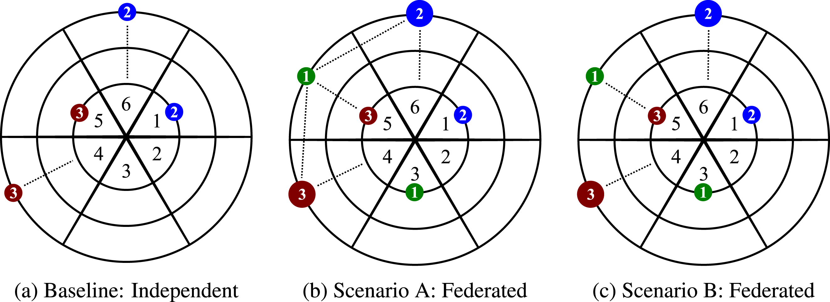
Figure 3. Initial ground station and satellite locations in a two-dimensional space numbered by player for (a) baseline, (b) scenario A, and (c) scenario B. Dotted lines indicate SGL or ISL for the initial conditions.
Table 7 shows the expected net present value for each strategic context using a discount rate of 2
![]() $\%$
per turn evaluated using 1000 seeded runs of the multi-actor value function. For clarity in presentation, players are assumed to be risk neutral such that expected net present value is equivalent to utility; however, alternative assumptions of risk attitudes would modify the resulting payoff values following a nonlinear utility curve. In practice, sensitivity analyses may help understand how unknown behavioral quantities such as risk attitudes influence results.
$\%$
per turn evaluated using 1000 seeded runs of the multi-actor value function. For clarity in presentation, players are assumed to be risk neutral such that expected net present value is equivalent to utility; however, alternative assumptions of risk attitudes would modify the resulting payoff values following a nonlinear utility curve. In practice, sensitivity analyses may help understand how unknown behavioral quantities such as risk attitudes influence results.
Table 7. Orbital federates design scenarios
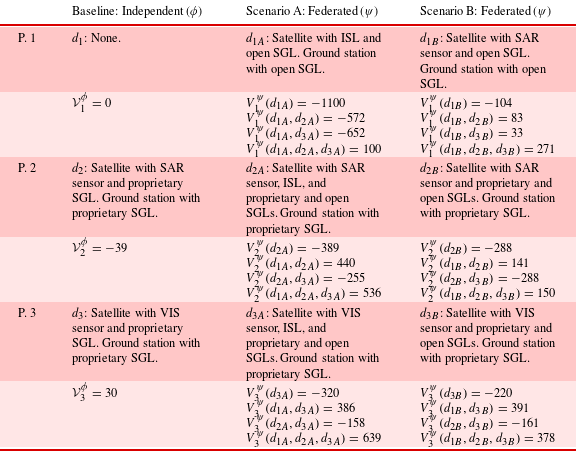
Table 8. Strategic design game for scenario A
4.2 Risk dominance analysis of scenario A
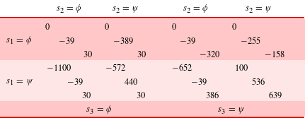
Table 8 populates a strategic design game for federated scenario A which constitutes a bipolar game with asymmetric players. Using Eq. (7), the normalized deviation losses are
 $$\begin{eqnarray}u=\left[\begin{array}{@{}c@{}}u_{1}\\ u_{2}\\ u_{3}\end{array}\right]=\left[\begin{array}{@{}c@{}}0.917\\ 0.378\\ 0.365\end{array}\right].\end{eqnarray}$$
Using Eq. (10), the linearized influence matrix is
 $$\begin{eqnarray}A=\left[\begin{array}{@{}ccc@{}}0 & \bar{a}_{12} & \bar{a}_{13}\\ \bar{a}_{21} & 0 & \bar{a}_{23}\\ \bar{a}_{31} & \bar{a}_{32} & 0\end{array}\right]=\left[\begin{array}{@{}ccc@{}}0 & 0.533 & 0.467\\ 0.876 & 0 & 0.124\\ 0.784 & 0.216 & 0\end{array}\right].\end{eqnarray}$$
Incentive function linearization error analysis using Eq. (9) shows small errors for all three players:
![]() $\unicode[STIX]{x1D700}=\left[0.047,0.010,0.024\right]$
.
$\unicode[STIX]{x1D700}=\left[0.047,0.010,0.024\right]$
.
Eigenvector analysis of the transposed influence matrix
![]() $A^{\intercal }$
yields the eigenvector (rescaled to unit norm)
$A^{\intercal }$
yields the eigenvector (rescaled to unit norm)
 $$\begin{eqnarray}w(A)=\left[\begin{array}{@{}c@{}}w_{1}(A)\\ w_{2}(A)\\ w_{3}(A)\end{array}\right]=\left[\begin{array}{@{}c@{}}0.455\\ 0.296\\ 0.249\end{array}\right]\end{eqnarray}$$
corresponding to the unit eigenvalue. Computing WALM as
shows the independent strategy
![]() $\unicode[STIX]{x1D719}$
to be risk dominant.
$\unicode[STIX]{x1D719}$
to be risk dominant.
Normalized deviation losses show the independent strategy is preferred for player 1 in all but high probabilities of collaboration (
![]() $u_{1}=0.917$
) because of large downside losses incurred if no other players choose the collective strategy. This risk fundamentally arises because player 1 has no independent source of revenue to recover the high cost of the federated design. However, the collective strategy has a lower threshold of collaboration for players 2 and 3 (
$u_{1}=0.917$
) because of large downside losses incurred if no other players choose the collective strategy. This risk fundamentally arises because player 1 has no independent source of revenue to recover the high cost of the federated design. However, the collective strategy has a lower threshold of collaboration for players 2 and 3 (
![]() $u_{2}=0.378,u_{3}=0.365$
) because large upside gains realized from shared data services overcome the additional cost of larger spacecraft and extra modules.
$u_{2}=0.378,u_{3}=0.365$
) because large upside gains realized from shared data services overcome the additional cost of larger spacecraft and extra modules.
Weighting factors identify player 1 as the most influential (
![]() $w_{1}=0.455$
) which can be explained by their central role in both providing shared ISL relay and SGL downlink services via the spacecraft and ground station, respectively. Smaller but similar weights for players 2 and 3 (
$w_{1}=0.455$
) which can be explained by their central role in both providing shared ISL relay and SGL downlink services via the spacecraft and ground station, respectively. Smaller but similar weights for players 2 and 3 (
![]() $w_{2}=0.296,w_{3}=0.249$
) reflect their similarity in operational mission.
$w_{2}=0.296,w_{3}=0.249$
) reflect their similarity in operational mission.
Given player 1’s aversion to the collective strategy and strong influence, the independent strategy is risk dominant in this design scenario. In particular, the collective strategy is prone to failure due to disengagement by player 1. A visualization of value surfaces in Figure 4 emphasizes the disparity between players 1 compared to 2 and 3 with respect to overall stability of the collective strategy.

Figure 4. Value surfaces for independent strategy
![]() $\unicode[STIX]{x1D719}_{i}$
versus collective strategy
$\unicode[STIX]{x1D719}_{i}$
versus collective strategy
![]() $\unicode[STIX]{x1D713}_{i}$
under federated scenario A. The independent strategy
$\unicode[STIX]{x1D713}_{i}$
under federated scenario A. The independent strategy
![]() $\unicode[STIX]{x1D719}$
is more dominant for player 1 while the collective strategy
$\unicode[STIX]{x1D719}$
is more dominant for player 1 while the collective strategy
![]() $\unicode[STIX]{x1D713}$
is more dominant for players 2 and 3.
$\unicode[STIX]{x1D713}$
is more dominant for players 2 and 3.
Table 9. Strategic design game for scenario B
4.3 Risk dominance analysis of scenario B
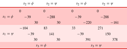
Table 9 populates a strategic design game for the federated scenario B which constitutes a bipolar game with asymmetric players. Using Eq. (7), the normalized deviation losses are
 $$\begin{eqnarray}u=\left[\begin{array}{@{}c@{}}u_{1}\\ u_{2}\\ u_{3}\end{array}\right]=\left[\begin{array}{@{}c@{}}0.277\\ 0.568\\ 0.418\end{array}\right].\end{eqnarray}$$
Using in Eq. (10), the linearized influence matrix is
 $$\begin{eqnarray}A=\left[\begin{array}{@{}ccc@{}}0 & \bar{a}_{12} & \bar{a}_{13}\\ \bar{a}_{21} & 0 & \bar{a}_{23}\\ \bar{a}_{31} & \bar{a}_{32} & 0\end{array}\right]=\left[\begin{array}{@{}ccc@{}}0 & 0.566 & 0.434\\ 0.990 & 0 & 0.010\\ 0.962 & 0.038 & 0\end{array}\right].\end{eqnarray}$$
Incentive function linearization error analysis using Eq. (9) shows small errors for all three players:
![]() $\unicode[STIX]{x1D700}=\left[0.034,0.005,0.030\right]$
.
$\unicode[STIX]{x1D700}=\left[0.034,0.005,0.030\right]$
.
Eigenvector analysis of the transposed influence matrix
![]() $A^{\intercal }$
yields the eigenvector (rescaled to unit norm)
$A^{\intercal }$
yields the eigenvector (rescaled to unit norm)
 $$\begin{eqnarray}w(A)=\left[\begin{array}{@{}c@{}}w_{1}(A)\\ w_{2}(A)\\ w_{3}(A)\end{array}\right]=\left[\begin{array}{@{}c@{}}0.494\\ 0.288\\ 0.217\end{array}\right]\end{eqnarray}$$
corresponding to the unit eigenvalue. Computing WALM as
shows the collective strategy
![]() $\unicode[STIX]{x1D713}$
is risk dominant.
$\unicode[STIX]{x1D713}$
is risk dominant.
Normalized deviation losses show the collective strategy is preferred for player 1 for a wide range of probabilities of collaboration (
![]() $u_{1}=0.277$
). The threshold for collaboration is higher for players 2 and 3 (
$u_{1}=0.277$
). The threshold for collaboration is higher for players 2 and 3 (
![]() $u_{2}=0.568,u_{3}=0.418$
) compared to scenario A. The goal of reducing upfront costs and providing an independent source of revenue successfully changed the strategic risk posture of player 1. However, the loss of ISL relay services and associated revenue disincentivize the collective strategy for players 2 and 3.
$u_{2}=0.568,u_{3}=0.418$
) compared to scenario A. The goal of reducing upfront costs and providing an independent source of revenue successfully changed the strategic risk posture of player 1. However, the loss of ISL relay services and associated revenue disincentivize the collective strategy for players 2 and 3.
Weighting factors still identify player 1 as the most influential (
![]() $w_{1}=0.494$
) and more influential compared to scenario A. Player 1 retains a key role in providing downlink services and, without ISL services among players 2 and 3, takes an even stronger role because other players lack the relay components to interact with each other directly. Players 2 and 3 retain similar weights (
$w_{1}=0.494$
) and more influential compared to scenario A. Player 1 retains a key role in providing downlink services and, without ISL services among players 2 and 3, takes an even stronger role because other players lack the relay components to interact with each other directly. Players 2 and 3 retain similar weights (
![]() $w_{2}=0.288,w_{3}=0.217$
) though both are less influential than in scenario A.
$w_{2}=0.288,w_{3}=0.217$
) though both are less influential than in scenario A.
Combining these factors, the collective strategy is risk dominant in this design scenario. This result indicates scenario B has preferable strategic dynamics to scenario A at the cost of slightly lower value. Notably, in the event that player 2 disengages, players 1 and 3 still enjoy moderate returns from the collective strategy. A visualization of value surfaces in Figure 5 shows a clear difference for player 1 compared to scenario A in Figure 4.
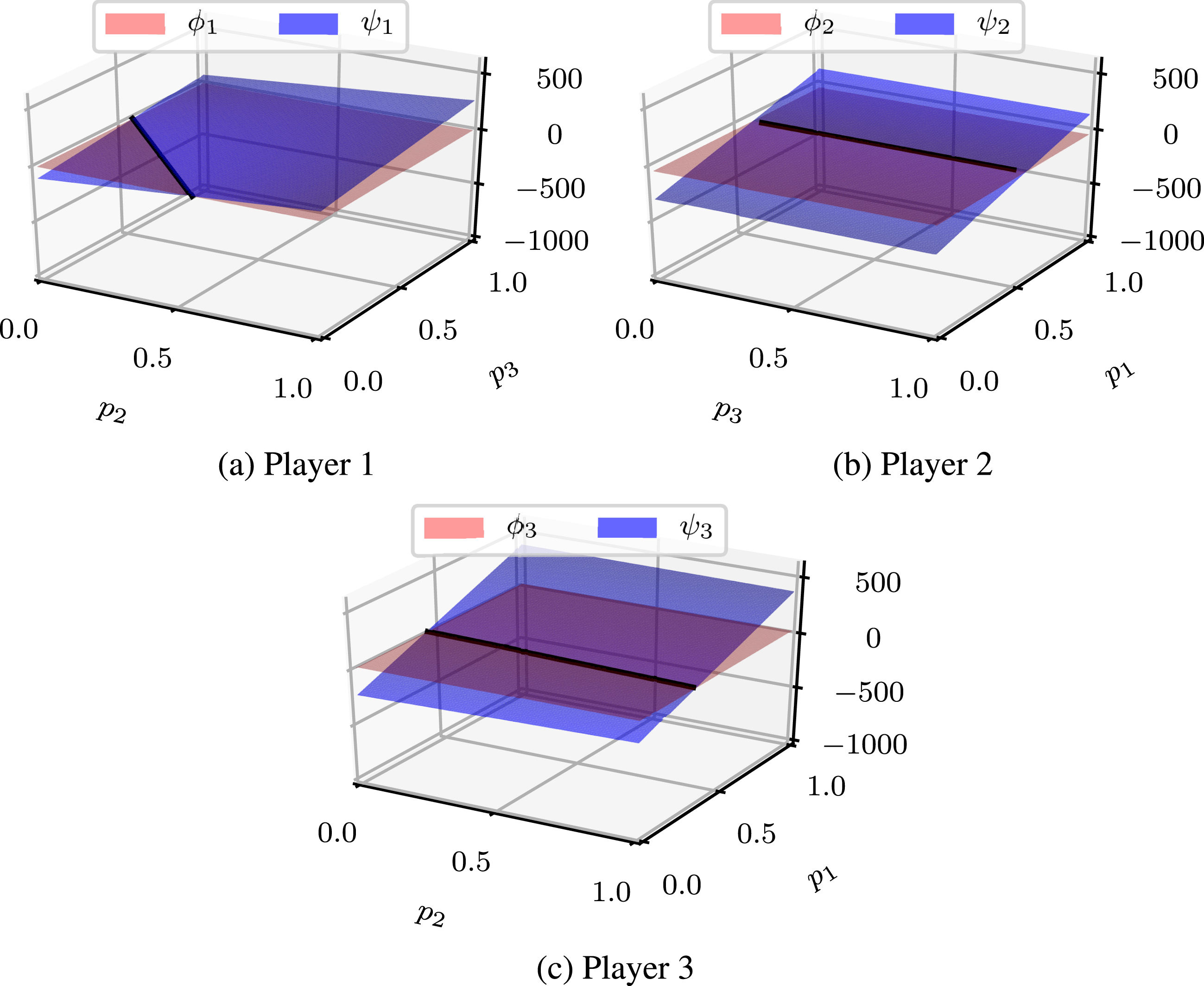
Figure 5. Value surfaces for independent strategy
![]() $\unicode[STIX]{x1D719}_{i}$
versus collective strategy
$\unicode[STIX]{x1D719}_{i}$
versus collective strategy
![]() $\unicode[STIX]{x1D713}_{i}$
under federated scenario B. The independent strategy
$\unicode[STIX]{x1D713}_{i}$
under federated scenario B. The independent strategy
![]() $\unicode[STIX]{x1D719}$
is dominant for player 2 while the collective strategy
$\unicode[STIX]{x1D719}$
is dominant for player 2 while the collective strategy
![]() $\unicode[STIX]{x1D713}$
is dominant for players 1 and 3.
$\unicode[STIX]{x1D713}$
is dominant for players 1 and 3.
4.4 Comparative analysis of results
This case illustrates how high-value (but also high-risk) designs emerge from optimization-oriented activities and how analysis of risk dominance has the potential to mitigate strategic instabilities by selecting more conservative alternatives. If successful, scenario A provides superior value for all three players by taking advantage of new technology and operational concepts. However, focusing on maximizing upside potential can yield unstable design solutions more susceptible to coordination failures. Player 1 experiences a significantly higher threshold for collaboration than others under scenario A and is most likely to disengage from a collective strategy.
Scenario B reduces the level of technological ambition and establishes an independent value source for all players. While its potential payoffs are smaller than A, scenario B exhibits superior strategic stability and is robust to disengagement by player 2, the most likely to disengage from a collective strategy. These results echo Maier’s principles for system-of-systems architecting emphasizing stable intermediate forms and ensuring cooperating among all actors (Maier Reference Maier1998). Risk dominance helps assess designs for a balance between value maximization if successful and risk minimization for coordination failures.
Although not considered in this analysis for clarity in presentation, incorporating risk attitudes would influence the absolute (but not relative) interpretation of risk dominance across scenarios A and B. For example, an exponential utility function of the form
![]() $U(c)=(1-e^{-\unicode[STIX]{x1D6FC}c})/\unicode[STIX]{x1D6FC}$
for consumption level
$U(c)=(1-e^{-\unicode[STIX]{x1D6FC}c})/\unicode[STIX]{x1D6FC}$
for consumption level
![]() $c$
, equivalent to expected net present value in this example, assumes constant risk aversion for
$c$
, equivalent to expected net present value in this example, assumes constant risk aversion for
![]() $\unicode[STIX]{x1D6FC}>0$
(Arrow Reference Arrow1971). Applying this transformation to the payoff values in Table 7 penalizes the high-value (but uncertain) collaborative outcomes and increases risk dominance measures across both scenarios. More detailed analysis would benefit from specific knowledge about risk attitudes on behalf of individual players.
$\unicode[STIX]{x1D6FC}>0$
(Arrow Reference Arrow1971). Applying this transformation to the payoff values in Table 7 penalizes the high-value (but uncertain) collaborative outcomes and increases risk dominance measures across both scenarios. More detailed analysis would benefit from specific knowledge about risk attitudes on behalf of individual players.
Alternative probabilistic analysis methods may evaluate expected value and variance under uncertain strategy selections. For example, defining
![]() $p_{i}$
as the probability player
$p_{i}$
as the probability player
![]() $i$
deviates from
$i$
deviates from
![]() $\unicode[STIX]{x1D719}$
to
$\unicode[STIX]{x1D719}$
to
![]() $\unicode[STIX]{x1D713}$
, the value function
$\unicode[STIX]{x1D713}$
, the value function
![]() $V_{i}$
is
$V_{i}$
is
 $$\begin{eqnarray}\displaystyle V_{i}(p_{i},p_{j},p_{k}) & = & \displaystyle {\mathcal{V}}_{i}^{\unicode[STIX]{x1D719}}(1-p_{i})+V_{i}^{\unicode[STIX]{x1D713}}(d_{i})p_{i}(1-p_{j})(1-p_{k})\nonumber\\ \displaystyle & & \displaystyle +\,V_{i}^{\unicode[STIX]{x1D713}}(d_{i},d_{k})p_{i}(1-p_{j})p_{k}+V_{i}^{\unicode[STIX]{x1D713}}(d_{i},d_{j})p_{i}p_{j}(1-p_{k})\nonumber\\ \displaystyle & & \displaystyle +\,V_{i}^{\unicode[STIX]{x1D713}}(d_{i},d_{j},d_{k})p_{i}p_{j}p_{k}.\end{eqnarray}$$
Assuming
![]() $p_{i}$
are independent and identically distributed with
$p_{i}$
are independent and identically distributed with
![]() $p_{i}\sim \text{uniform}(0,1)$
, Table 10 reports expected value
$p_{i}\sim \text{uniform}(0,1)$
, Table 10 reports expected value
![]() $E\left[V_{i}\right]$
and variance
$E\left[V_{i}\right]$
and variance
![]() $\text{Var}(V_{i})$
for scenarios A and B. The analysis concurs that player 1 in scenario A and player 2 in scenario B observe negative expected value and scenario B overall decreases variance for all players. However, this analysis: 1) does not provide any tradeoff between expected value and variance, 2) only provides a relative comparison between the two cases without a scalar quantitative metric of stability, and 3) does not provide further insights for the interdependency or influence between or among players.
$\text{Var}(V_{i})$
for scenarios A and B. The analysis concurs that player 1 in scenario A and player 2 in scenario B observe negative expected value and scenario B overall decreases variance for all players. However, this analysis: 1) does not provide any tradeoff between expected value and variance, 2) only provides a relative comparison between the two cases without a scalar quantitative metric of stability, and 3) does not provide further insights for the interdependency or influence between or among players.
Table 10. Comparative analysis of expected value and variance

5 Discussion and conclusion
Understanding of both the upside potential and downside risk associated with coordination failures are critical to assess sources of strategic risk in collaborative systems. As demonstrated in the application case, the concepts of strategic design games and measures of risk dominance can influence concept selection in early design activities by identifying unfavorable strategic dynamics and shifting the design focus to include economic stability in addition to economic efficiency.
The core contributions of this paper establish: 1) a method to formulate and measure strategic risk dominance for collaborative engineered systems with two or more asymmetric players and 2) a linear approximation to incentives required for problems with more than two players. This work extends prior work on multi-actor value functions (Grogan et al. Reference Grogan, Ho, Golkar and de Weck2018) and transfers fundamental economic theory to the domain of systems engineering to study issues of strategic risk dominance in multi-actor systems.
Building on equilibrium selection literature and WALM as a quantitative metric to assess risk dominance provide a solid foundation for strategic design games. The relative simplicity of the proposed method permits analysis of strategic dynamics during conceptual design, allowing systems engineers to identify, avoid, or rework high-value joint architectures that carry unfavorable strategic dynamics. This perspective may help avoid costly development programs with structural problems leading to schedule and cost growth and, ultimately, cancelation. However, there remain several key assumptions regarding linearized incentive structures and information availability discussed in Section 3.3 which limit more detailed analysis of strategic dynamics in engineering design.
Future work follows two directions. First, additional theoretical work to incorporate concepts from Bayesian games would help bring subjective information into context-specific design problems. Second, additional practical or applied work is required to further validate the proposed method in a realistic system context by developing a multi-actor value function, enumerating and evaluating candidate architectures to identify those with desirable strategic dynamics, and contextualize results by selectively forming and dissolving coalitions.
Acknowledgments
Thanks to Abbas Ehsanfar for his initial efforts and general contributions to exploring this topic. This material is based on work supported, in whole or in part, by the U.S. Department of Defense through the Systems Engineering Research Center (SERC) under Contract No. HQ0034-13-D-0004. SERC is a federally funded University Affiliated Research Center managed by Stevens Institute of Technology. Any opinions, findings, and conclusions or recommendations expressed in this material are those of the authors and do not necessarily reflect the views of the United States Department of Defense.
Appendix A. Detailed WALM formulation
This section summarizes key results from Selten (Reference Selten1995) to formulate and explain the weighted average log measure (WALM) of risk dominance. It does not produce any new results but introduces some more convenient notation and insights. Please refer to the original article for axioms and proofs.
Binary games have a strategy space with two alternatives
![]() ${\mathcal{S}}_{i}=\{\unicode[STIX]{x1D719}_{i},\unicode[STIX]{x1D713}_{i}\}$
. Bipolar games are a subclass of binary games with two Nash equilibria defined by shared strategies among all players
${\mathcal{S}}_{i}=\{\unicode[STIX]{x1D719}_{i},\unicode[STIX]{x1D713}_{i}\}$
. Bipolar games are a subclass of binary games with two Nash equilibria defined by shared strategies among all players
![]() $\unicode[STIX]{x1D719}=(\unicode[STIX]{x1D719}_{1},\ldots ,\unicode[STIX]{x1D719}_{n})$
and
$\unicode[STIX]{x1D719}=(\unicode[STIX]{x1D719}_{1},\ldots ,\unicode[STIX]{x1D719}_{n})$
and
![]() $\unicode[STIX]{x1D713}=(\unicode[STIX]{x1D713}_{1},\ldots ,\unicode[STIX]{x1D713}_{n})$
. Note that, for example,
$\unicode[STIX]{x1D713}=(\unicode[STIX]{x1D713}_{1},\ldots ,\unicode[STIX]{x1D713}_{n})$
. Note that, for example,
![]() $\unicode[STIX]{x1D719}$
denotes the strategy set and
$\unicode[STIX]{x1D719}$
denotes the strategy set and
![]() $\unicode[STIX]{x1D719}_{i}$
denotes the strategy selected by player
$\unicode[STIX]{x1D719}_{i}$
denotes the strategy selected by player
![]() $i$
. Notation with negative subscripts on strategy sets denotes non-participation, for example,
$i$
. Notation with negative subscripts on strategy sets denotes non-participation, for example,
![]() $\unicode[STIX]{x1D719}_{-1}=(\unicode[STIX]{x1D713}_{1},\unicode[STIX]{x1D719}_{2},\ldots ,\unicode[STIX]{x1D719}_{n})$
. Without loss of generality, this section labels strategy sets such that
$\unicode[STIX]{x1D719}_{-1}=(\unicode[STIX]{x1D713}_{1},\unicode[STIX]{x1D719}_{2},\ldots ,\unicode[STIX]{x1D719}_{n})$
. Without loss of generality, this section labels strategy sets such that
![]() $\unicode[STIX]{x1D713}$
is payoff dominant as the collective strategy.
$\unicode[STIX]{x1D713}$
is payoff dominant as the collective strategy.
For greater generality, WALM of risk dominance is defined in terms of a biform that describes the essential dynamics of a game rather than the direct payoff or utility function. The biform is given by a vector of normalized deviation losses
![]() $u=u(\unicode[STIX]{x1D719},\unicode[STIX]{x1D713})=\left[u_{i}(\unicode[STIX]{x1D719},\unicode[STIX]{x1D713})\right]$
and an influence matrix
$u=u(\unicode[STIX]{x1D719},\unicode[STIX]{x1D713})=\left[u_{i}(\unicode[STIX]{x1D719},\unicode[STIX]{x1D713})\right]$
and an influence matrix
![]() $A=A(\unicode[STIX]{x1D719},\unicode[STIX]{x1D713})=\left[a_{ij}(\unicode[STIX]{x1D719},\unicode[STIX]{x1D713})\right]$
capturing interdependencies between players.Footnote
1
Together, these factors attribute potential losses to global and local deviations from a baseline strategy.
$A=A(\unicode[STIX]{x1D719},\unicode[STIX]{x1D713})=\left[a_{ij}(\unicode[STIX]{x1D719},\unicode[STIX]{x1D713})\right]$
capturing interdependencies between players.Footnote
1
Together, these factors attribute potential losses to global and local deviations from a baseline strategy.
The most intuitive explanation of risk dominance starts by formulating an incentive function
![]() $D_{i}$
for player
$D_{i}$
for player
![]() $i$
to choose
$i$
to choose
![]() $\unicode[STIX]{x1D719}_{i}$
over
$\unicode[STIX]{x1D719}_{i}$
over
![]() $\unicode[STIX]{x1D713}_{i}$
. Player
$\unicode[STIX]{x1D713}_{i}$
. Player
![]() $i$
prefers
$i$
prefers
![]() $\unicode[STIX]{x1D719}_{i}$
for
$\unicode[STIX]{x1D719}_{i}$
for
![]() $D_{i}>0$
and prefers
$D_{i}>0$
and prefers
![]() $\unicode[STIX]{x1D713}_{i}$
for
$\unicode[STIX]{x1D713}_{i}$
for
![]() $D_{i}<0$
. An expected value expression expanded in Eq. (21) describes the incentive function from a global perspective as a function of
$D_{i}<0$
. An expected value expression expanded in Eq. (21) describes the incentive function from a global perspective as a function of
![]() $p$
, the probability that all other players choose
$p$
, the probability that all other players choose
![]() $\unicode[STIX]{x1D713}$
.
$\unicode[STIX]{x1D713}$
.
 $$\begin{eqnarray}\displaystyle D_{i}(p) & \propto & \displaystyle E\left[V_{i}|\unicode[STIX]{x1D719}_{i}\right]-E\left[V_{i}|\unicode[STIX]{x1D713}_{i}\right]\nonumber\\ \displaystyle & = & \displaystyle \left[V_{i}(\unicode[STIX]{x1D719})(1-p)+V_{i}(\unicode[STIX]{x1D713}_{-i})p\right]-\left[V_{i}(\unicode[STIX]{x1D719}_{-i})(1-p)+V_{i}(\unicode[STIX]{x1D713})p\right]\nonumber\\ \displaystyle & = & \displaystyle V_{i}(\unicode[STIX]{x1D719})-V_{i}(\unicode[STIX]{x1D719}_{-i})-\left[V_{i}(\unicode[STIX]{x1D719})-V_{i}(\unicode[STIX]{x1D719}_{-i})+V_{i}(\unicode[STIX]{x1D713})-V_{i}(\unicode[STIX]{x1D713}_{-i})\right]p.\qquad\end{eqnarray}$$
Equation (22) defines deviation loss
![]() $L_{i}$
as a function of a strategy set
$L_{i}$
as a function of a strategy set
![]() $\unicode[STIX]{x1D709}\in \{\unicode[STIX]{x1D719},\unicode[STIX]{x1D713}\}$
up to a constant of proportionality.
$\unicode[STIX]{x1D709}\in \{\unicode[STIX]{x1D719},\unicode[STIX]{x1D713}\}$
up to a constant of proportionality.
The deviation loss captures sensitivity to deviating away from a stable strategy set through one’s own actions; however, for the purpose of this formulation consider it an algebraic expression only. The normalized deviation loss
![]() $u_{i}$
in Eq. (23) transforms
$u_{i}$
in Eq. (23) transforms
![]() $L_{i}$
to a unit scale.
$L_{i}$
to a unit scale.
Returning to the global incentive function, Eq. (24) normalizes both sides and substitutes expressions for
![]() $L_{i}$
and
$L_{i}$
and
![]() $u_{i}$
to achieve a simplified incentive function.
$u_{i}$
to achieve a simplified incentive function.
In other words, player
![]() $i$
prefers
$i$
prefers
![]() $\unicode[STIX]{x1D719}_{i}$
for
$\unicode[STIX]{x1D719}_{i}$
for
![]() $D_{i}>0\;\Longleftrightarrow \;p<u_{i}$
and prefers
$D_{i}>0\;\Longleftrightarrow \;p<u_{i}$
and prefers
![]() $\unicode[STIX]{x1D713}_{i}$
for
$\unicode[STIX]{x1D713}_{i}$
for
![]() $D_{i}<0\;\Longleftrightarrow \;p>u_{i}$
. The normalized deviation loss
$D_{i}<0\;\Longleftrightarrow \;p>u_{i}$
. The normalized deviation loss
![]() $u_{i}$
(also referred to as the diagonal probability
$u_{i}$
(also referred to as the diagonal probability
![]() $\unicode[STIX]{x1D70B}_{i}$
in literature) marks the intersection between the lines in Figure 6 where
$\unicode[STIX]{x1D70B}_{i}$
in literature) marks the intersection between the lines in Figure 6 where
![]() $D_{i}(u_{i})=0$
(i.e. player
$D_{i}(u_{i})=0$
(i.e. player
![]() $i$
is indifferent about which strategy to select).
$i$
is indifferent about which strategy to select).
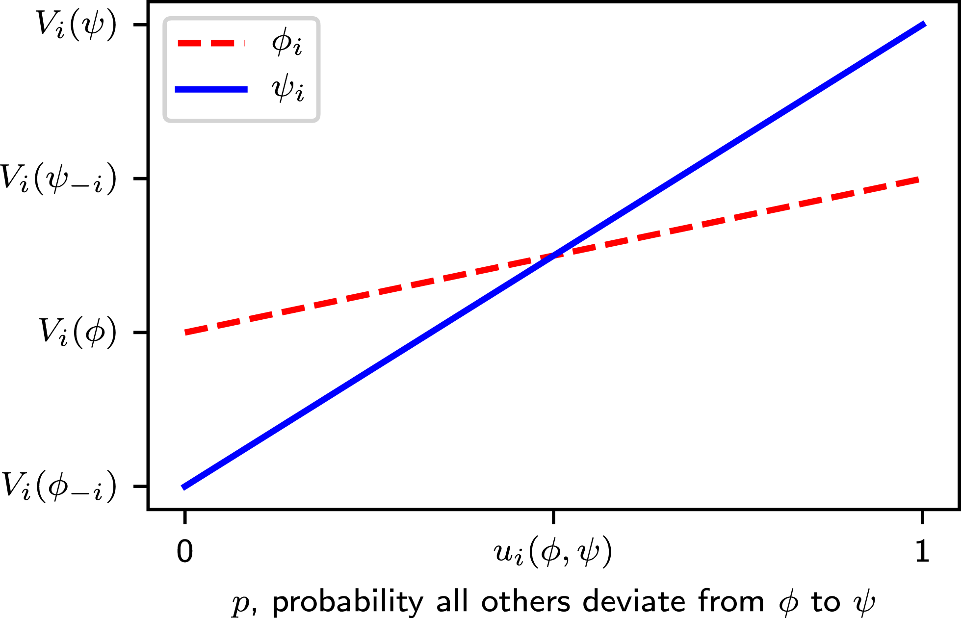
Figure 6. The normalized deviation loss in bipolar games marks the intersection between strategy-specific value functions shown here for player
![]() $i$
as a function of
$i$
as a function of
![]() $p$
, the probability that all others deviate from
$p$
, the probability that all others deviate from
![]() $\unicode[STIX]{x1D719}$
to
$\unicode[STIX]{x1D719}$
to
![]() $\unicode[STIX]{x1D713}$
.
$\unicode[STIX]{x1D713}$
.
A more detailed incentive function can be written from a local perspective specific to each players’ strategy to capture interaction effects and interdependencies. An expected value expression expanded in Eq. (25) for a game with
![]() $n=3$
players describes the incentive function as a function of
$n=3$
players describes the incentive function as a function of
![]() $p_{j}$
and
$p_{j}$
and
![]() $p_{k}$
, the probability that players
$p_{k}$
, the probability that players
![]() $i$
and
$i$
and
![]() $j$
choose
$j$
choose
![]() $\unicode[STIX]{x1D713}_{i}$
and
$\unicode[STIX]{x1D713}_{i}$
and
![]() $\unicode[STIX]{x1D713}_{k}$
, respectively.
$\unicode[STIX]{x1D713}_{k}$
, respectively.
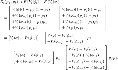 $$\begin{eqnarray}\displaystyle & & \displaystyle D_{i}(p_{j},p_{k})\propto E\left[V_{i}|\unicode[STIX]{x1D719}_{i}\right]-E\left[V_{i}|\unicode[STIX]{x1D713}_{i}\right]\nonumber\\ \displaystyle & & \displaystyle \quad =\left[\begin{array}{@{}ll@{}} & V_{i}(\unicode[STIX]{x1D719})(1-p_{j})(1-p_{k})\\ & +V_{i}(\unicode[STIX]{x1D719}_{-j})p_{j}(1-p_{k})\\ & +V_{i}(\unicode[STIX]{x1D719}_{-k})(1-p_{j})p_{k}\\ & +V_{i}(\unicode[STIX]{x1D713}_{-i})p_{j}p_{k}\end{array}\right]-\left[\begin{array}{@{}ll@{}} & V_{i}(\unicode[STIX]{x1D719}_{-i})(1-p_{j})(1-p_{k})\\ & +V_{i}(\unicode[STIX]{x1D719}_{-ij})p_{j}(1-p_{k})\\ & +V_{i}(\unicode[STIX]{x1D719}_{-ik})(1-p_{j})p_{k}\\ & +V_{i}(\unicode[STIX]{x1D713})p_{j}p_{k}\end{array}\right]\nonumber\\ \displaystyle & & \displaystyle \quad =\left[V_{i}(\unicode[STIX]{x1D719})-V_{i}(\unicode[STIX]{x1D719}_{-i})\right]-\left[\begin{array}{@{}ll@{}} & V_{i}(\unicode[STIX]{x1D719})-V_{i}(\unicode[STIX]{x1D719}_{-i})\\ & +V_{i}(\unicode[STIX]{x1D719}_{-ij})-V_{i}(\unicode[STIX]{x1D719}_{-j})\end{array}\right]p_{j}\nonumber\\ \displaystyle & & \displaystyle \qquad -\,\left[\begin{array}{@{}ll@{}} & V_{i}(\unicode[STIX]{x1D719})-V_{i}(\unicode[STIX]{x1D719}_{-i})\\ & +V_{i}(\unicode[STIX]{x1D719}_{-ik})-V_{i}(\unicode[STIX]{x1D719}_{-k})\end{array}\right]p_{k}-\left[\begin{array}{@{}ll@{}} & V_{i}(\unicode[STIX]{x1D713})-V_{i}(\unicode[STIX]{x1D713}_{-i})\\ & -V_{i}(\unicode[STIX]{x1D719})+V_{i}(\unicode[STIX]{x1D719}_{-i})\\ & +V_{i}(\unicode[STIX]{x1D719}_{-j})-V_{i}(\unicode[STIX]{x1D719}_{-ij})\\ & +V_{i}(\unicode[STIX]{x1D719}_{-k})-V_{i}(\unicode[STIX]{x1D719}_{-ik})\end{array}\right]p_{j}p_{k}.\qquad\end{eqnarray}$$
Equation (26) defines pairwise deviation loss
![]() $L_{ij}$
as a function of a strategy set
$L_{ij}$
as a function of a strategy set
![]() $\unicode[STIX]{x1D709}\in \{\unicode[STIX]{x1D719},\unicode[STIX]{x1D713}\}$
up to a constant of proportionality.
$\unicode[STIX]{x1D709}\in \{\unicode[STIX]{x1D719},\unicode[STIX]{x1D713}\}$
up to a constant of proportionality.
Similar to deviation loss, pairwise deviation loss captures sensitivity to deviating away from a stable strategy set through pairwise actions but for the purpose of this formulation consider it an algebraic expression only. Influence elements
![]() $a_{ij}$
in Eq. (27) normalize pairwise deviation losses
$a_{ij}$
in Eq. (27) normalize pairwise deviation losses
![]() $L_{ij}$
to a common scale with
$L_{ij}$
to a common scale with
![]() $u_{i}$
.
$u_{i}$
.
Returning to the local incentive function, normalizing both sides yields the simplified form in Eq. (28).
 $$\begin{eqnarray}\displaystyle D_{i}(p_{j},p_{k}) & = & \displaystyle \frac{1}{L_{i}(\unicode[STIX]{x1D719})+L_{i}(\unicode[STIX]{x1D713})}\nonumber\\ \displaystyle & & \displaystyle \times \,\left[\begin{array}{@{}ll@{}} & L_{i}(\unicode[STIX]{x1D719})-\left(L_{i}(\unicode[STIX]{x1D719})-L_{ij}(\unicode[STIX]{x1D719})\right)p_{j}-\left(L_{i}(\unicode[STIX]{x1D719})-L_{ik}(\unicode[STIX]{x1D719})\right)p_{k}\\ & -\left(L_{i}(\unicode[STIX]{x1D713})-L_{i}(\unicode[STIX]{x1D719})+L_{ij}(\unicode[STIX]{x1D719})+L_{ik}(\unicode[STIX]{x1D719})\right)p_{j}p_{k}\end{array}\right]\nonumber\\ \displaystyle & = & \displaystyle u_{i}-a_{ij}p_{j}-a_{ik}p_{k}-\left(1-a_{ij}-a_{ik}\right)p_{j}p_{k}.\end{eqnarray}$$
Under the assumption of linear incentives,
![]() $1-a_{ij}-a_{ik}=0$
such that
$1-a_{ij}-a_{ik}=0$
such that
![]() $D=u-Ap$
which is the general result applicable to games with any number of players.
$D=u-Ap$
which is the general result applicable to games with any number of players.
Finally, influence weights measure the overall importance of one player on others’ stability. Weights
![]() $w=\left[w_{i}(A)\right]$
are defined implicitly by properties in Eq. (29) based on the influence matrix
$w=\left[w_{i}(A)\right]$
are defined implicitly by properties in Eq. (29) based on the influence matrix
![]() $A=\left[a_{ij}\right]$
.
$A=\left[a_{ij}\right]$
.
Weights are interpreted as the eigenvector (rescaled to unit norm) of
![]() $A^{\intercal }$
corresponding to the unit eigenvalue, guaranteed to exist by the assumption of linear incentives which forces the row sum of
$A^{\intercal }$
corresponding to the unit eigenvalue, guaranteed to exist by the assumption of linear incentives which forces the row sum of
![]() $A$
to unity for all rows. Note that weights are equivalent to the limiting stochastic distribution for the Markov chain with state transition probabilities
$A$
to unity for all rows. Note that weights are equivalent to the limiting stochastic distribution for the Markov chain with state transition probabilities
![]() $a_{ij}$
.
$a_{ij}$
.
Appendix B. Approximation to linear incentives
Selten’s work focuses on games with linear incentives which allow pairwise interactions to be quantified without third party effects (e.g. the effect of player
![]() $j$
on player
$j$
on player
![]() $i$
is not a function of player
$i$
is not a function of player
![]() $k$
). This simplifying assumption, similar to a first order approximation, greatly reduces complexity for a narrow class of problems but cannot directly represent increasing or decreasing returns to scale (i.e. network effects) common in engineering applications. Furthermore, linear incentives is a critical assumption to find weighting factors which require a unit eigenvalue of the influence matrix
$k$
). This simplifying assumption, similar to a first order approximation, greatly reduces complexity for a narrow class of problems but cannot directly represent increasing or decreasing returns to scale (i.e. network effects) common in engineering applications. Furthermore, linear incentives is a critical assumption to find weighting factors which require a unit eigenvalue of the influence matrix
![]() $A$
. Although there may be extensions of the influence matrix
$A$
. Although there may be extensions of the influence matrix
![]() $A$
to higher dimensions (e.g. tensors), there is currently no such existing theory. Thus, this section introduces a novel linear approximation for greater applicability to design problems with nonlinear incentives.
$A$
to higher dimensions (e.g. tensors), there is currently no such existing theory. Thus, this section introduces a novel linear approximation for greater applicability to design problems with nonlinear incentives.
Linear incentives can be visualized as planar value surfaces in Figure 7 for a game with
![]() $n=3$
players as a function of
$n=3$
players as a function of
![]() $p_{j}$
and
$p_{j}$
and
![]() $p_{k}$
, the probability players
$p_{k}$
, the probability players
![]() $j$
and
$j$
and
![]() $k$
choose strategy
$k$
choose strategy
![]() $\unicode[STIX]{x1D713}$
over
$\unicode[STIX]{x1D713}$
over
![]() $\unicode[STIX]{x1D719}$
, respectively. The incentive function
$\unicode[STIX]{x1D719}$
, respectively. The incentive function
![]() $D_{i}(p_{j},p_{k})$
is the difference between the two planes. The intersection between the two planes (black line) traces the indifference curve where player
$D_{i}(p_{j},p_{k})$
is the difference between the two planes. The intersection between the two planes (black line) traces the indifference curve where player
![]() $i$
does not prefer either strategy, similar to
$i$
does not prefer either strategy, similar to
![]() $u_{i}$
for
$u_{i}$
for
![]() $n=2$
players. Games with nonlinear incentives visualized in Figure 7 for an exaggerated case include interaction terms with third parties and yield non-planar value surfaces and nonlinear indifference curves.
$n=2$
players. Games with nonlinear incentives visualized in Figure 7 for an exaggerated case include interaction terms with third parties and yield non-planar value surfaces and nonlinear indifference curves.
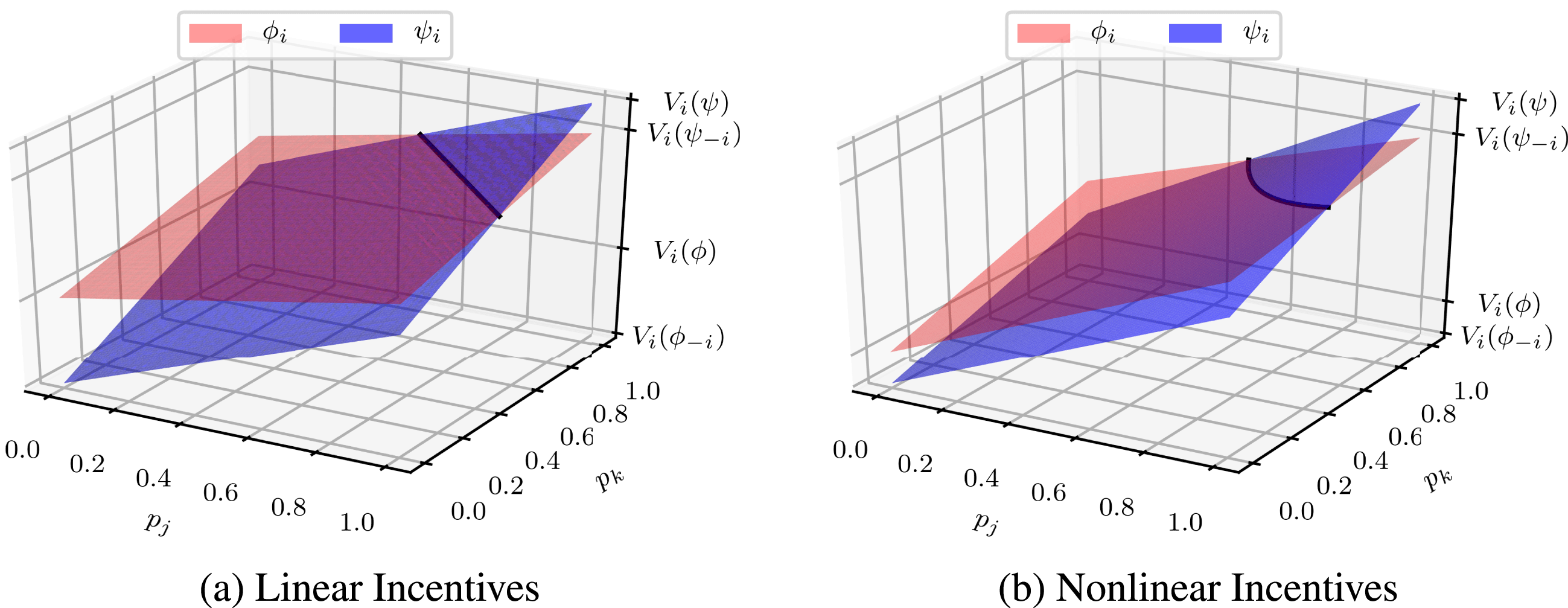
Figure 7. Value surfaces for player
![]() $i$
as a function of player
$i$
as a function of player
![]() $j$
’s and
$j$
’s and
![]() $k$
’s probability of choosing
$k$
’s probability of choosing
![]() $\unicode[STIX]{x1D713}_{j}$
and
$\unicode[STIX]{x1D713}_{j}$
and
![]() $\unicode[STIX]{x1D713}_{k}$
(
$\unicode[STIX]{x1D713}_{k}$
(
![]() $p_{j}$
and
$p_{j}$
and
![]() $p_{k}$
). Linear incentives produce planar value surfaces while nonlinear incentives produce non-planar (curved) surfaces representing third party effects.
$p_{k}$
). Linear incentives produce planar value surfaces while nonlinear incentives produce non-planar (curved) surfaces representing third party effects.
Consider the simplest possible game with nonlinear incentives with
![]() $n=3$
players and incentive function in Eq. (28). Linear incentives require
$n=3$
players and incentive function in Eq. (28). Linear incentives require
![]() $a_{ij}+a_{ik}=1$
to eliminate the interaction term between
$a_{ij}+a_{ik}=1$
to eliminate the interaction term between
![]() $p_{j}$
and
$p_{j}$
and
![]() $p_{k}$
. A linearized incentive function in Eq. (1) proposes modified
$p_{k}$
. A linearized incentive function in Eq. (1) proposes modified
![]() $a_{ij}$
terms such that
$a_{ij}$
terms such that
![]() $\sum _{j=1}^{n}\bar{a}_{ij}=1\;\forall \;i$
to satisfy the linear incentives condition.
$\sum _{j=1}^{n}\bar{a}_{ij}=1\;\forall \;i$
to satisfy the linear incentives condition.
Preserving influence elements as a coefficient for the effect of player
![]() $j$
’s probability of choosing
$j$
’s probability of choosing
![]() $\unicode[STIX]{x1D713}_{j}$
on player
$\unicode[STIX]{x1D713}_{j}$
on player
![]() $i$
’s incentive to choose
$i$
’s incentive to choose
![]() $\unicode[STIX]{x1D719}_{i}$
(specifically,
$\unicode[STIX]{x1D719}_{i}$
(specifically,
![]() $-\unicode[STIX]{x2202}D_{i}/\unicode[STIX]{x2202}p_{j}$
), Eq. (2) defines the linearized influence element
$-\unicode[STIX]{x2202}D_{i}/\unicode[STIX]{x2202}p_{j}$
), Eq. (2) defines the linearized influence element
![]() $\bar{a}_{ji}$
as the expected value of the partial derivative of the incentive function with respect to
$\bar{a}_{ji}$
as the expected value of the partial derivative of the incentive function with respect to
![]() $p_{j}$
.
$p_{j}$
.
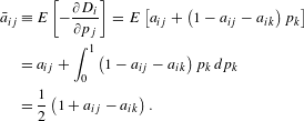 $$\begin{eqnarray}\displaystyle \bar{a}_{ij} & \equiv & \displaystyle E\left[-\frac{\unicode[STIX]{x2202}D_{i}}{\unicode[STIX]{x2202}p_{j}}\right]=E\left[a_{ij}+\left(1-a_{ij}-a_{ik}\right)p_{k}\right]\nonumber\\ \displaystyle & = & \displaystyle a_{ij}+\int _{0}^{1}\left(1-a_{ij}-a_{ik}\right)p_{k}\,dp_{k}\nonumber\\ \displaystyle & = & \displaystyle \frac{1}{2}\left(1+a_{ij}-a_{ik}\right).\end{eqnarray}$$
For more general games with
![]() $n>3$
players, linearizing incentive functions using this approximation becomes a combinatorial problem based on
$n>3$
players, linearizing incentive functions using this approximation becomes a combinatorial problem based on
![]() ${\mathcal{K}}_{ij}$
, the power set
${\mathcal{K}}_{ij}$
, the power set
![]() ${\mathcal{P}}$
of third parties (i.e. set of all subsets of players except
${\mathcal{P}}$
of third parties (i.e. set of all subsets of players except
![]() $i$
and
$i$
and
![]() $j$
and including the empty set) in Eq. (3) with cardinality
$j$
and including the empty set) in Eq. (3) with cardinality
![]() $|{\mathcal{K}}_{ij}|$
in Eq. (4) given by the binomial theorem.
$|{\mathcal{K}}_{ij}|$
in Eq. (4) given by the binomial theorem.
Revised notation in Eq. (5) defines combinatorial deviation losses between player
![]() $i$
and a set of players
$i$
and a set of players
![]() $\mathbf{k}$
as a function of a strategy set
$\mathbf{k}$
as a function of a strategy set
![]() $\unicode[STIX]{x1D709}\in \{\unicode[STIX]{x1D719},\unicode[STIX]{x1D713}\}$
up to a constant of proportionality.
$\unicode[STIX]{x1D709}\in \{\unicode[STIX]{x1D719},\unicode[STIX]{x1D713}\}$
up to a constant of proportionality.
Note that this expression simplifies to previously established forms of
![]() $L_{i\{\}}(\unicode[STIX]{x1D709})=L_{i}(\unicode[STIX]{x1D709})$
in Eq. (22) for
$L_{i\{\}}(\unicode[STIX]{x1D709})=L_{i}(\unicode[STIX]{x1D709})$
in Eq. (22) for
![]() $\mathbf{k}=\{\}$
and
$\mathbf{k}=\{\}$
and
![]() $L_{i\{j\}}(\unicode[STIX]{x1D709})=L_{ij}(\unicode[STIX]{x1D709})$
in Eq. (26) for
$L_{i\{j\}}(\unicode[STIX]{x1D709})=L_{ij}(\unicode[STIX]{x1D709})$
in Eq. (26) for
![]() $\mathbf{k}=\{j\}$
. Using this notation, Eq. (6) states a conjecture for linearized influence elements.
$\mathbf{k}=\{j\}$
. Using this notation, Eq. (6) states a conjecture for linearized influence elements.
While proof of this conjecture is not available, the result above has been manually verified for
![]() $n=3$
(see Eq. (2) recognizing that
$n=3$
(see Eq. (2) recognizing that
![]() $L_{ij}(\unicode[STIX]{x1D719})=-L_{ik}(\unicode[STIX]{x1D713})$
) and
$L_{ij}(\unicode[STIX]{x1D719})=-L_{ik}(\unicode[STIX]{x1D713})$
) and
![]() $n=4$
cases.
$n=4$
cases.

Figure 8. Incentive function
![]() $D_{i}(p_{j},p_{k})$
for player
$D_{i}(p_{j},p_{k})$
for player
![]() $i$
as a function of
$i$
as a function of
![]() $p_{j}$
and
$p_{j}$
and
![]() $p_{k}$
for (a) nonlinear and (b) linearized cases with (c) difference
$p_{k}$
for (a) nonlinear and (b) linearized cases with (c) difference
![]() $\unicode[STIX]{x1D6FF}_{i}(p_{j},p_{k})$
and mean error
$\unicode[STIX]{x1D6FF}_{i}(p_{j},p_{k})$
and mean error
![]() $\unicode[STIX]{x1D700}_{i}=0.125$
.
$\unicode[STIX]{x1D700}_{i}=0.125$
.
Linearizing influence elements introduces errors into the risk dominance analysis. Error manifests as differences between the incentive function
![]() $D_{i}(p_{j},p_{k})$
and its linearized form in Eq. (7) for games with
$D_{i}(p_{j},p_{k})$
and its linearized form in Eq. (7) for games with
![]() $n=3$
players.
$n=3$
players.
 $$\begin{eqnarray}\displaystyle \unicode[STIX]{x1D6FF}_{i}(p_{j},p_{k}) & = & \displaystyle D_{i}(p_{j},p_{k})-\left(u_{i}-\bar{a}_{ij}p_{j}-\bar{a}_{ik}p_{k}\right)\nonumber\\ \displaystyle & = & \displaystyle \left(\bar{a}_{ij}-a_{ij}\right)p_{j}+\left(\bar{a}_{ik}-a_{ik}\right)p_{k}-\left(1-a_{ij}-a_{ik}\right)p_{j}p_{k}\nonumber\\ \displaystyle & = & \displaystyle \left(1-a_{ij}-a_{ik}\right)\left(\frac{p_{j}}{2}+\frac{p_{k}}{2}+p_{j}p_{k}\right).\end{eqnarray}$$
For example, Figure 8 visualizes contours of player
![]() $i$
’s incentive function for a notional symmetric
$i$
’s incentive function for a notional symmetric
![]() $n=3$
game with value function
$n=3$
game with value function
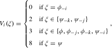 $$\begin{eqnarray}V_{i}(\unicode[STIX]{x1D709})=\left\{\begin{array}{@{}ll@{}}0\quad & \text{if }\unicode[STIX]{x1D709}=\unicode[STIX]{x1D719}_{-i}\\ 2\quad & \text{if }\unicode[STIX]{x1D709}\in \{\unicode[STIX]{x1D713}_{-k},\unicode[STIX]{x1D713}_{-j}\}\\ 3\quad & \text{if }\unicode[STIX]{x1D709}\in \{\unicode[STIX]{x1D719},\unicode[STIX]{x1D719}_{-j},\unicode[STIX]{x1D719}_{-k},\unicode[STIX]{x1D713}_{-i}\}\\ 8\quad & \text{if }\unicode[STIX]{x1D709}=\unicode[STIX]{x1D713}\end{array}\right.,\end{eqnarray}$$
influence elements
![]() $a_{ij}=0.25$
, and linearized influence elements
$a_{ij}=0.25$
, and linearized influence elements
![]() $\bar{a}_{ij}=0.5$
for (a) initially (highly) nonlinear incentives, (b) linearized incentives following the recommended method, and (c) the subsequent absolute difference
$\bar{a}_{ij}=0.5$
for (a) initially (highly) nonlinear incentives, (b) linearized incentives following the recommended method, and (c) the subsequent absolute difference
![]() $\unicode[STIX]{x1D6FF}_{i}$
.
$\unicode[STIX]{x1D6FF}_{i}$
.
Equation (9) derives a simple error metric
![]() $\unicode[STIX]{x1D700}_{i}$
for cases with
$\unicode[STIX]{x1D700}_{i}$
for cases with
![]() $n=3$
players that measures the average absolute difference in incentive value.
$n=3$
players that measures the average absolute difference in incentive value.
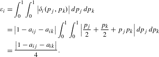 $$\begin{eqnarray}\displaystyle \unicode[STIX]{x1D700}_{i} & = & \displaystyle \int _{0}^{1}\int _{0}^{1}\left|\unicode[STIX]{x1D6FF}_{i}(p_{j},p_{k})\right|dp_{j}\,dp_{k}\nonumber\\ \displaystyle & = & \displaystyle \left|1-a_{ij}-a_{ik}\right|\int _{0}^{1}\int _{0}^{1}\left|\frac{p_{j}}{2}+\frac{p_{k}}{2}+p_{j}p_{k}\right|dp_{j}\,dp_{k}\nonumber\\ \displaystyle & = & \displaystyle \frac{\left|1-a_{ij}-a_{ik}\right|}{4}.\end{eqnarray}$$
Note that
![]() $D_{i}(p_{j},p_{k})\in \left[u_{i}-1,u_{i}\right]$
so
$D_{i}(p_{j},p_{k})\in \left[u_{i}-1,u_{i}\right]$
so
![]() $\unicode[STIX]{x1D700}_{i}$
can be roughly interpreted as percent error. For the example in Figure 8,
$\unicode[STIX]{x1D700}_{i}$
can be roughly interpreted as percent error. For the example in Figure 8,
![]() $\unicode[STIX]{x1D700}_{i}=0.125$
which is a relatively high value indicating potential errors in interpreting results, especially in regions with high estimates of one partner’s probability of collaboration but low estimates for the other.
$\unicode[STIX]{x1D700}_{i}=0.125$
which is a relatively high value indicating potential errors in interpreting results, especially in regions with high estimates of one partner’s probability of collaboration but low estimates for the other.
Appendix C. Application case data
Data for the application case was generated using the publicly available distribution of Orbital Federates Simulation – Python (OFSPY) (Grogan Reference Grogan2019). This software simulation computes cash flows obtained from an initial space systems design in a version of the multi-player game Orbital Federates. The software program contains a command line interface (CLI) to run specific design scenarios. Automated operational policies based on mixed integer linear programs determine how to use available space systems to observe, store, transmit, and downlink data to complete contracts and earn revenue each turn.
The spatial context is reduced to two dimensions with six sectors (1–6) and layers representing the surface (SUR), low Earth orbit (LEO), and medium Earth orbit (MEO) shown in Figure 9. Satellites move clockwise between orbital sectors each turn while ground stations remain fixed at the surface. Space-to-ground links (SGLs) require a satellite to be in the same sector as a ground station for data transfer. Inter-satellite links (ISLs) require satellites to be in adjacent sectors for data transfer. Proprietary links only permit data transfer within a player’s assets while open links permit data transfer between players as paid services.
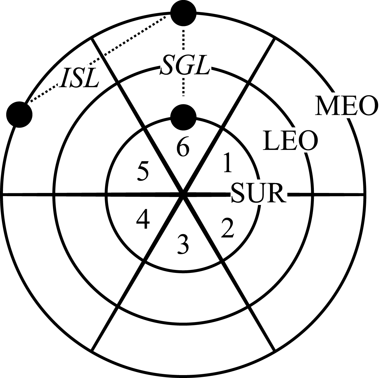
Figure 9. The Orbital Federates context includes six sectors with surface (SUR), low Earth orbit (LEO) and medium Earth orbit (MEO) layers. Satellite and ground station elements transfer data using space-to-ground (SGL) and inter-satellite (ISL) links.
Designs evaluated under the independent strategy follow the CLI template: ofs.py -d 24 -p 3 -i 0 -s <SEED> -o d6,a,1 -f n <DESIGN> where -d 24 indicates a game with 24 turns, -p 3 indicates three players, -i 0 indicates no initial cash constraints, -s <SEED> indicates the random number generator seed (integer), -o d6,a,1 indicates to use a dynamic operations policy with a six turn horizon using an automatically computed opportunity cost for storage and a nominal penalty of 1 for ISLs, -f n indicates no federation operations policy, and <DESIGN> is the design specification.
The baseline scenario considers the design specification:
(i) 2.SmallSat@MEO6,SAR,pSGL 2.GroundSta@SUR1,pSGL
(ii) 3.SmallSat@MEO4,VIS,pSGL 3.GroundSta@SUR5,pSGL
Player 1 has no elements. Player 2 has a small satellite initially in MEO sector 6 with a synthetic aperture radar (SAR) and proprietary SGL (pSGL) and a ground station at surface sector 1 with a pSGL. Player 3 has a small satellite initially in MEO sector 4 with a visual light sensor (VIS) and pSGL and a ground station at surface sector 5 with a pSGL.
Designs evaluated under the collective strategy follow the CLI template: ofs.py -d 24 -p 3 -i 0 -s <SEED> -o d6,a,1 -f x100,100,6,a,1 <DESIGN> where -f x100,100,6,a,1 indicates to use an opportunistic federation operations policy with fixed prices of 100 for SGL and ISL, a six turn horizon, an automatically computed opportunity cost for storage, and a nominal penalty of 1 for ISLs.
Scenario A considers the design specification:
(i) 1.SmallSat@MEO5,oISL,oSGL 1.GroundSta@SUR3,oSGL
(ii) 2.MediumSat@MEO6,SAR,oISL,pSGL,oSGL 2.GroundSta@SUR1,pSGL
(iii) 3.MediumSat@MEO4,VIS,oISL,pSGL,oSGL 3.GroundSta@SUR5,pSGL
Player 1 has a small satellite in MEO sector 5 with an open ISL (oISL) and an open SGL (oSGL) and a ground station at surface sector 3 with oSGL. Player 2 has a medium satellite in MEO sector 6 with SAR, oISL, pSGL, and oSGL and a ground station at surface sector 1 with pSGL. Player 3 has a medium satellite in MEO sector 4 with VIS, oISL, pSGL, and OSGL and a ground station at surface sector 5 with pSGL.
Scenario B considers the design specification:
(i) 1.SmallSat@MEO5,SAR,oSGL 1.GroundSta@SUR3,oSGL
(ii) 2.MediumSat@MEO6,SAR,pSGL,oSGL 2.GroundSta@SUR1,pSGL
(iii) 3.MediumSat@MEO4,VIS,pSGL,oSGL 3.GroundSta@SUR5,pSGL
Player 1 has a small satellite in MEO sector 5 with SAR and oSGL and a ground station at surface sector 3 with oSGL. Players 2 and 3 are identical to Scenario A except removing the oISL modules.
Note that scenario A relies on close proximity between players to enable ISLs. The above design strings were modified in cases with only partial participation in the federation: MEO5 is replaced by MEO3 if only players 1 and 3 join a federation and MEO4 is replaced by MEO5 if only players 2 and 3 join a federation. Outputs reported in Table 7 compute net present values using a discount rate of 2% (per turn) averaged over the first 1000 seeds (from 0 to 999).
