Variation and change in the productivity of be going to V in the Corpus of Historical American English, 1810–2009

Abstract

This article focuses on the poster child of grammaticalization, be going to V. First expressing ‘motion with intention’, in Early Modern English the construction came to signify ‘motionless intention’. The grammaticalization process continued in Late Modern English with subjectification, so that ‘intention’ was gradually replaced by ‘prediction’. We study the process from Late Modern to Present-Day English in the 200-million-word fiction section of the Corpus of Historical American English (COHA), 1810–2009, for which we have gender metadata on the authors. We focus on the productivity of the construction by comparing type frequencies, i.e., the number of different verbs following be going to. Our research questions are how the grammaticalization is reflected in the productivity of the construction, and whether the social factor of gender played a role in the process. We study the internal factors of mental verbs, inanimate subjects and passive voice; to this end, we use robust statistical methods to compare type frequencies and proportions of types over time. We also investigate the semantics of the verb types by drawing on techniques from distributional semantics. Our wider aim is to enrich the cognitively oriented theory of Construction Grammar with insights from historical sociolinguistics.

1. Introduction

Our article focuses on the poster child of grammaticalization, be going to V (e.g. Bybee & Pagliuca 1987; Danchev & Kytö 1994; Hopper & Traugott 2003; Hilpert 2008; Traugott & Trousdale 2013; Budts & Petré 2016; Petré & Van de Velde 2018). First expressing ‘motion with intention’, as in I’m going to the market to buy bananas, in Early Modern English the construction came to signify ‘motionless intention’, as in I’m going to read your work tomorrow. The grammaticalization process continued in Late Modern English with subjectification, so that ‘intention’ was gradually replaced by ‘prediction’, as in There’s going to be some serious trouble here (Budts & Petré 2016). Wu et al. (2016) conducted a quantitative analysis of the grammaticalization of be going to V in the Corpus of Historical American English (COHA), 1810–2009. They found that the frequency of the construction continued to increase in COHA from Late Modern to Present-Day English, also in terms of the use of mental verbs, inanimate subjects and passive voice, all of which can be linked to the ‘prediction’ sense.

We study this juncture in the 200-million-word fiction section of COHA, using gender metadata developed by Öhman et al. (2019). Whereas Wu et al. (2016) analysed the grammaticalization process in terms of token frequency, we focus on the productivity of the construction by comparing type frequencies, i.e. the number of different verbs following be going to. Our research questions are how the grammaticalization is reflected in the productivity of the construction, and whether the social factor of gender played a role in the process. Following Wu et al. (2016), we study the internal factors of mental verbs, inanimate subjects and passive voice; we also investigate the semantics of the verb types by drawing on techniques from distributional semantics (Perek 2016), which allows us to measure the semantic spread of the construction at different points in time. To compare type frequencies and proportions of types over time and across factors, we use robust statistical methods building upon the work of Rodríguez-Puente et al. (2022) and Säily et al. (2024).

Although the research reported in this study is not dependent on any particular theoretical framework, our wider aim is to enrich the cognitively oriented theory of Diachronic Construction Grammar (DCxG; e.g. Traugott & Trousdale 2013) with insights from historical sociolinguistics. Studies in both present-day and historical sociolinguistics have found the social category of gender to be key in language change. In particular, it is often women who tend to lead language change (e.g. Labov 2001: 262; Nevalainen & Raumolin-Brunberg 2003: 131). Previous sociolinguistic work on variation and change in morphological productivity, however, has tended to show a male advantage (e.g. Säily 2014), the reasons for which are as yet unclear. It is therefore of interest to study the patterning of gender in the productivity of syntactic constructions as well, particularly in combination with language-internal factors (cf. Säily et al. 2024).

The rest of this article is organized as follows. Section 2 surveys previous research on the construction, while section 3 discusses our material. Section 4 presents our methods and analysis, and section 5 concludes the article with a discussion of the results and their implications for future research.

2. Background

Movement is one of the main sources of future constructions cross-linguistically (e.g. Bybee & Pagliuca 1987: 110–11; this also applies to temporal adverb constructions, as in Silvennoinen 2025). Bybee & Pagliuca (1987: 116–18) propose that the meaning of be going to V grammaticalized from concrete movement to figurative movement (including a sense of intention) and ultimately to prediction, similarly to many other future constructions (Bybee et al. 1991: 32). Hopper & Traugott (2003: 2–3) argue that the starting point of the process was a directional use that already included a sense of intention or purpose. Budts & Petré (2016: 2, 16) provide examples of the stages of grammaticalization of the construction, summarized in (1)–(3) below.

Previous research indicates that the ‘motionless intention’ sense arose in Early Modern English by the late seventeenth century (e.g. Danchev & Kytö 1994; Núñez Pertejo 1999), while the ‘prediction’ sense developed in Late Modern to Present-Day English (e.g. Budts & Petré 2016; Wu et al. 2016). The stages overlap, and in fact all of the senses still coexist today, which is not the case with all movement-based future constructions (Traugott 2012: 241). Rather than absolute distinctions, the change therefore chiefly operates on the relative proportions of the different senses, as also noted by Danchev & Kytö (1994: 68–9). In DCxG terms, the emergence of the motionless intention sense corresponds to an instance of constructionalization (Traugott & Trousdale 2013), i.e. the creation of a new form–meaning pair in the network of constructions and its conventionalization across the speech community. In other words, the be going to V pattern comes to be directly associated with the meaning of intention found in instances of go as a motion verb such as (1), and thus loses the entailment of motion. As discussed by Traugott & Trousdale (2013), constructionalization is typically followed by constructional changes, i.e. changes in the form of the construction (e.g. reduction), its meaning (in particular semantic bleaching), and its productivity.

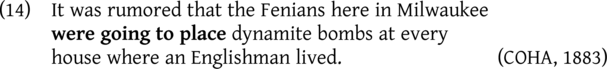
The semantic change of the be going to V construction from intention to prediction can be regarded as a process of subjectification, by which constructions begin to be used to express the speaker’s attitudes and beliefs (Traugott 2010: 33). The subjectification of be going to V in Late Modern English was analysed in a relatively large-scale empirical study by Budts & Petré (2016), who found in the Corpus of Late Modern English Texts (CLMET) a number of indicators of change from the late eighteenth to the early nineteenth century. These included a decrease in first-person subjects and imminent future contexts (I am going to entrust you with a secret) as well as an increase in non-agentive subjects and infinitival complements expressing events of low agentivity (It’s going to rain; our example from COHA, 1811).

Wu et al. (2016) also examined the later development of the construction, focusing on American English in COHA from the nineteenth century onwards. They investigated the frequencies of mental verbs, the inanimate subject it and passive voice in the construction over time, as in (4)–(6) (our examples). All of these can be linked to the change from intention to prediction, as ‘this usage decreases the intention and purposiveness of the subject as well as the directionality of the verb go’ (Wu et al. 2016: 321). Wu et al. (2016) found that the frequencies of these contexts increased throughout the time period covered by the corpus, from 1810 to 2009, which to us indicates continued grammaticalization, even if Wu et al. (2016: 324) consider the construction to have been ‘fully grammaticalized’ in the late seventeenth century, as determined by the first occurrence of mental verbs in the construction in their Google Books data. ¹

It has often been noted that changes in the meaning of a grammaticalizing construction are typically correlated with what Himmelmann (2004: 32) terms ‘host-class expansion’, i.e. an increase in the range of lexical items attested in the slots of the construction. In a DCxG approach, these changes may directly follow from semantic change in the construction: as the meaning of a construction becomes more schematic, a wider set of lexical items become compatible with it and may thus be used in the construction (Perek 2018, 2020). An example of this for the be going to V construction is the case of mental verbs investigated by Wu et al. (2016), as already mentioned above: mental predicates such as forget and amuse do not easily lend themselves to the original ‘motion with intention’ meaning of the be going to V pattern, or to the newly grammaticalized meaning ‘motionless intention’. Hence, their occurrence in the construction speaks to the increased availability of the more abstract prediction sense. Importantly, host-class expansion does not typically occur abruptly but is rather gradual and probabilistic (Traugott & Trousdale 2013: 114–15), hence it can be documented in diachronic corpora. Mental verbs are but one example of host-class expansion in be going to V; more broadly, Hilpert (2008: 119–21) reports from a diachronic distinctive collexeme analysis of the construction in CLMET that verbs with high agentivity such as fight and speak are most prominent in the earlier periods of the corpus (i.e. eighteenth to mid nineteenth century), while more schematic verbs like be, do, have and verbs referring to non-intentional events like die and happen are most distinctive of the last period (see also Budts & Petré 2016: 20–1). However, while these studies do confirm the grammaticalization path of be going to V through some of its distributional changes, a more detailed description of host-class expansion in the history of construction is lacking.

We build upon the work of Budts & Petré (2016) and Wu et al. (2016) by considering two hitherto unexamined perspectives on the process in Late Modern and Present-Day English. First, we focus on changes in the productivity of the construction, in terms of overall type frequencies of the verb slot, the proportions of types occurring in the three contexts exemplified in (4)–(6) above, as well as host-class expansion, in terms of new semantic types of verbs joining the distribution of the construction. ² Second, we combine our constructional approach with historical sociolinguistics by considering the influence of gender on the change. For this purpose, we utilize the fiction section of COHA, which has identifiable authors.

3. Material

We use the first version of COHA (Davies 2010–), which contains approximately 400 million words from the period 1810–2009. Aside from it being the version to which our institutions had access, the choice of the first version was motivated by comparability with previous research (Wu et al. 2016) as well as by the availability of fiction-specific genre and gender metadata for this version (see below). The instances of the construction were retrieved from the downloadable version of the corpus licensed by the University of Helsinki, which makes the data more easily accessible but has the downside that 5 per cent of the tokens, or ten consecutive words in every 200 words, have been replaced with @ signs for copyright reasons. ³ The corpus nevertheless remains usable for linguistic research, and its large size enables the study of lower-frequency constructions over time.

COHA is divided into four genres: fiction (c. 50 per cent of the data), magazines, newspapers and other non-fiction. As fiction is usually written by identifiable authors, it was used as the basis for our sociolinguistic study. Furthermore, fiction represents informal language use with elements of speech-like interaction (Culpeper & Kytö 2010: 16–18), where many kinds of language change are expected to show up earlier than in more formal genres. The fiction section of COHA comes with metadata on the names of the authors, although these are not in a completely consistent format. This metadata was used by Öhman et al. (2019) to generate gender information for the authors. ⁴ The identification was based on extracting the first names of the authors, which were then compared with historical parish records as well as modern name lists using a machine learning approach to label the author as male or female, with uncertain cases labelled as unknown. This resulted in a highly accurate classification which enabled Öhman et al. (2019) to discover consistent gender patterns in the use of the indefinite pronouns -body and -one over time. For the present study, we did some further spot-checking and manually corrected the coding of the ambiguous name Robin, and one case in which the author was a husband-and-wife pair, for which we set the gender to unknown. The size of the fiction dataset for which gender is known is c. 186 million words out of a total of 197 million words.

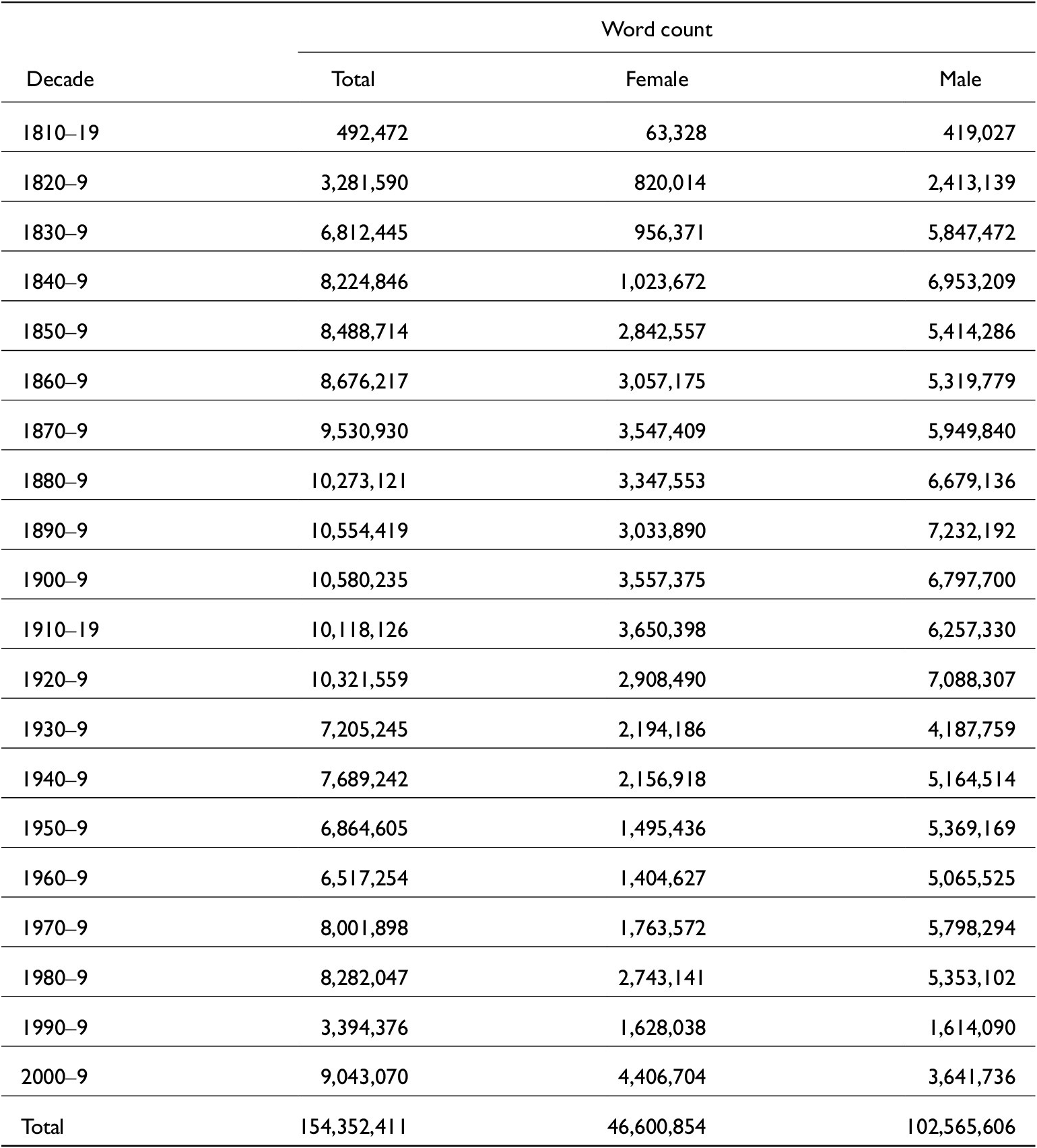
There are, however, some issues with the balance of the fiction section of COHA, in that different kinds of fiction are unevenly distributed over time. While novels form the majority of the corpus, it also contains for instance short stories, drama and movie scripts, the proportion of which increases in the twentieth century. Säily & Vartiainen (forthcoming) noticed that this skewed their results on the change from much -ed to very -ed, so that there seemed to be a gender difference in the latter part of the corpus which disappeared when the dataset was restricted to novels alone. Following their lead, we have decided to restrict our dataset to novels only. The size of this dataset by gender and decade is shown in table 1. Note that for most of our analyses we use a sliding window of forty years with ten-year increments: the forty-year window ensures that we have enough data for each window position, while moving it by such a small increment enables us to more accurately identify periods of significant variation and change.

Table 1. Size of the dataset by decade and author gender. Total word counts include authors of unknown gender

We acknowledge that the use of this dataset to analyse gender differences in language change is somewhat problematic. The dataset is not a socially representative or balanced corpus of American men and women’s language use in 1810–2009; rather, it represents the language use of the highly selective group of published authors of fiction included in COHA, the sampling of which has been influenced by such issues as availability and copyright. Moreover, the language use in novels varies not only by the gender of the author, but also by the gender of the characters as well as by subgenre, on which we have no metadata. Nevertheless, as novels tend to be informal and speech-like, and there are plenty of them in the corpus, this is arguably the best dataset currently available for the gender-based analysis of this 200-year stretch of American English. Encouraged by the results of Öhman et al. (2019), we embrace Labov’s (1994: 11) definition of historical linguistics as ‘the art of making the best use of bad data’ and proceed with our analysis, while keeping the limitations of the dataset in mind and returning to them in section 5.

Our data retrieval and cleanup process was as follows. We used the ‘database form’ of COHA, ⁵ including the ‘db’, ‘lexicon’ and ‘sources’ (metadata) files. We combined the metadata from the database with fiction-specific genre metadata provided in the ‘cohaTexts.xls’ file downloaded from the English-Corpora.org site, as well as with the gender metadata produced by Öhman et al. (2019). We did some manual cleanup of the metadata as described above and turned it into a machine-readable (JSON) form.

To find relevant instances of the construction, we automatically extracted data from the COHA database files using a Rust program. The search query was VB*, “going”, “to”, V?I*. We also searched for the gonna form (“gon”, “na”, *), which emerges in the 1920s in the novels of our corpus and represents the final stage of grammaticalization of be going to V, in which the complex auxiliary has been reanalysed to a single morpheme (Hopper & Traugott 2003: 68), but the dataset ended up being too small for our study. ⁶ We then cleaned up the results for the fiction section manually in Excel. In total, 1,861 be going to V types were checked, and verb types like market, which was actually a noun (as in I was going to market to get some of the best fruit), were removed. In a later step, instances of the be-passive (defined as VB*, V?N) and get-passive (“get”, V?N) were classified and corrected so that the verb that was counted was the lexical verb, e.g. ask rather than be in was going to be asked. Other classifications added to the data were mental verbs (using a list from Halliday & Matthiessen (2014: 256–7), with ambiguous types like strike removed) and the inanimate subject it (defined as “it” at the end of the context preceding the node). Our software library for querying COHA, as well as the dataset with our classifications and metadata in a JSON format, are freely available for download. ⁷

4. Methods and analysis

4.1. Type frequencies

4.1.1. Challenges in analysing type frequencies

To study how the productivity of the be going to V construction has changed over time, we analyse type frequencies: we count how many different verbs follow be going to in each time period. However, here we face three main challenges.

First, we have vastly different amounts of text from different time periods, and different amounts of text from men and women (see table 1). Type frequencies cannot be directly compared across corpora of different sizes: for example, if a 1-million-word corpus has 100 different verbs in be going to V constructions, it is not at all obvious how many types we would expect in a 10-million-word corpus. Normalization is not an option because type frequencies grow nonlinearly with corpus size (Säily & Suomela 2009: 96–7).

Second, we would like to be able to make a distinction between the be going to V construction being used more frequently vs. it being used in a more diverse manner. Even if two texts have the same number of words, one of them might use be going to V more frequently but in a repetitive manner, while another one could use it less frequently but in a productive manner. Merely counting the number of types will miss this distinction.

Third, even if we had the same amount of data and the same token frequency, and we observed differences in the type frequencies, we would still need to be able to assess whether the differences are statistically significant.

4.1.2. Methods for analysing type frequencies

We address these challenges in our study by building upon the methodology developed by Säily & Suomela (2009, 2017), Rodríguez-Puente et al. (2022), and Säily et al. (2024). The methods build on the idea of resampling (more precisely, permutation testing): to assess whether women use be going to V in a significantly productive manner, we compare the number of types in the subcorpus that consists of women’s texts with the number of types in a randomly constructed subcorpus of the same size. For example, if we have 1 million words written by women and we have 100 different types in their texts, we can construct a random subcorpus with 1 million words and see if we get as many types there. We can repeat this process a large number of times, and this way conclude whether 100 types is an unusually high number in this corpus for a subcorpus of such length. We can directly assess the statistical significance of this finding by counting which fraction of random subcorpora have such a high number of types. For example, if fewer than 0.1 per cent of random subcorpora have at least as high a number of types as the texts written by women, then we can conclude that gender indeed is significant with p < 0.001 for a one-tailed test or with p < 0.002 for a two-tailed test; in the two-tailed version the null hypothesis is simply that gender is unrelated to type diversity. The numbers we report here are for a one-tailed test.

In a similar manner, we can construct a subcorpus of texts written in a certain time period, and assess whether the number of types there is unusually high or low in comparison with a random subcorpus of a similar size. Here random sampling is done at the level of texts (as opposed to sampling random words), to ensure that any single text cannot have a large impact on the results, and to ensure that the randomly constructed corpus contains meaningful textual units, similar to the original corpus.

A direct application of the above idea already addresses the first and third issues listed in section 4.1.1 above: we are comparing subcorpora of the same size, and by constructing a large number of random subcorpora we can assess statistical significance. However, the technique can also be adapted to different measures of corpus size: instead of sampling random subcorpora with a given number of running words, we can sample random subcorpora with a given token frequency of the target construction. This enables us to address the second issue.

4.1.3. The types3 software

For this work, we have developed a computer program that we call types3, which makes it possible to explore trends in type frequencies and to assess the statistical significance of the trends (see figure 1). The software loads a JSON file that describes the composition of the corpus – in our case, the JSON file lists all distinct texts of the corpus, and for each text it contains text-level metadata (e.g. the gender of the author) and a list of all instances of be going to V in the text. For each instance we have the lemmatized verb and possible token-level or type-level classifications (e.g. whether it is considered a mental verb). With types3 we can then start to explore the use of the construction from different perspectives: we can see not only the number of types but also the number of hapax legomena, and we can compare the numbers with random subcorpora that have the same number of running words or the same number of be going to V instances. These measures are similar to the productivity measures proposed by Baayen (1993, 2009) but designed for comparability across subcorpora of unequal size. To analyse the proportion of types of a specific kind (such as mental verbs) out of all types over time, we can also compare subcorpora with the same number of types. Finally, we can compare token frequencies of be going to V in subcorpora with the same number of running words. We can explore different periodizations, zoom into various subcorpora, and visualize the results both over time and across genders.

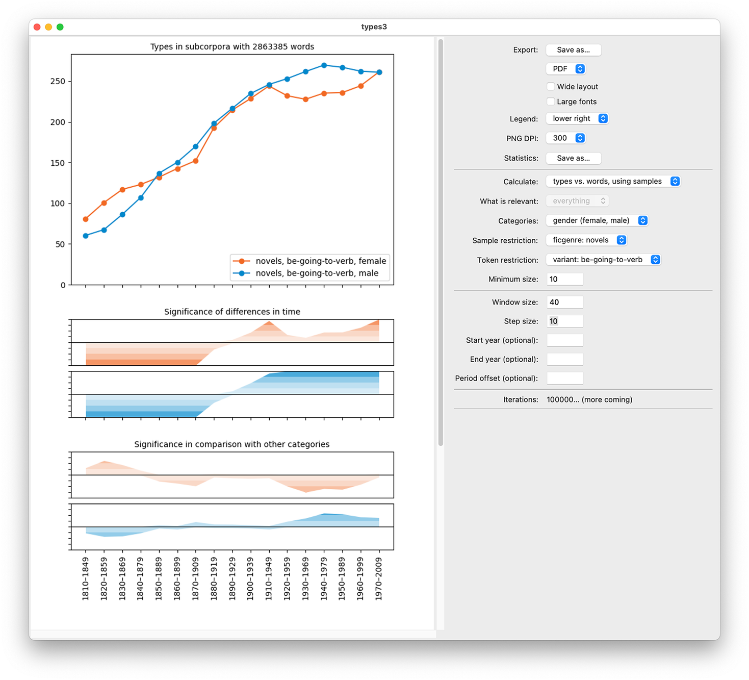
Figure 1. The user interface of types3 on macOS

In addition to the features discussed above, types3 differs from prior tools in terms of the user experience and the way the results are visualized and presented. First, the entire tool is developed for exploring variation in productivity over time, and all visualizations aim at providing a clear overview of diachronic trends and their statistical significance. Second, even though resampling statistics in general require a significant amount of computation (the results presented here are based on 1 million randomly constructed subcorpora), types3 makes it possible to conduct interactive exploration without doing any computation in advance: the user can adjust the settings, and approximate results based on a smaller number of random samples are presented almost instantly, while more accurate statistics are automatically computed in the background. The computationally intensive parts of the tool are written in Rust, while the user interface is written in Python; the program is freely available for download. ⁸

4.1.4. Overall trends

Figure 2 shows the results that we obtain when we compare the type frequencies of the verb slot in the be going to V construction in terms of the number of running words in the corpus. In the trend view on the left, types3 shows how the number of types evolves over time. The trend curve is computed as follows: First, we find the period with the smallest number of words; in this case it was the period 1810–49 with 18.8 million words. Then for each period we randomly reorder the texts, and see how many types we accumulate in the first 18.8 million words (and as the cutoff point is typically in the middle of a text, we record the number of types both before and after the final text). We repeat this process for each period 1 million times, and take the average number of types. This way we will get a trend curve that is useful for human inspection and easy to interpret: roughly speaking, it shows how many types we get if we take 18.8 million words of text from each period. This approach is similar to the one used by Berg (2021), and the idea of taking a sample of equal size from each subcorpus (though not the resampling and averaging) seems to have been first presented by Gaeta & Ricca (2006); see further Säily et al. (2024: 11).

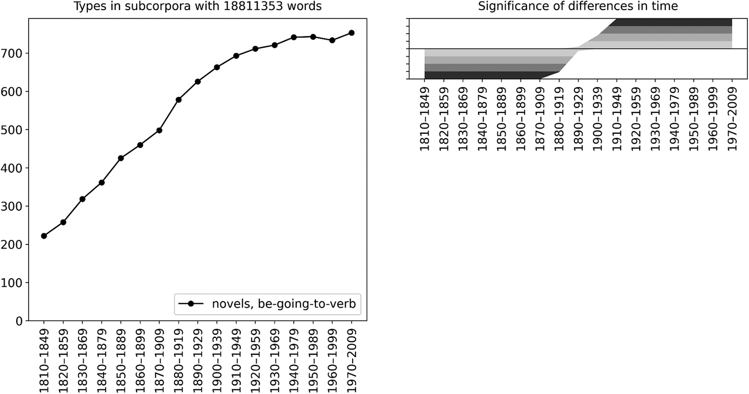
Figure 2. Change in the type frequency of be going to V by the number of running words in COHA novels

However, while there is a clear increase in the number of types in the trend curve, it does not yet tell us whether the findings are statistically significant – we would never expect a perfectly flat line in any real-world corpus, but is the trend that we see here strong enough that we can say it is unlikely to be a random artefact unrelated to any genuine diachronic trend? This is where we need the significance curve that is shown on the right in figure 2. Here we have used permutation testing for each period to test the following hypotheses: (1) the number of types in this period is significantly high in comparison with the corpus as a whole, and (2) the number of types in this period is significantly low in comparison with the corpus as a whole (the null hypothesis being that the time period of a text does not influence the number of types).

To do such testing for one period, for example, period 1940–79, we take all data that we have in this period (it turns out to be 29.1 million words and 916 types); note that this is different from the way the trend curve is produced. We then randomly sample texts from the entire corpus so that we accumulate a total of 29.1 million words, and calculate how many types we get that way. We repeat this process 1 million times and see how many times we get fewer than 916 types this way, and how many times we get more than 916 types this way (again keeping in mind that the exact cutoff point may be in the middle of a text, and we need to correct in the right direction so as not to overestimate significance). It turns out that almost all 29.1-million-word collections of text from the entire corpus have fewer than 916 types; we can conclude that the type diversity in 1940–79 is indeed significantly high in comparison with the corpus as a whole, with p < 0.0001. This is indicated in the significance plot with the dark shading for 1940–79; different shades correspond to p = 0.1, 0.01, 0.001, and 0.0001. We can see from the significance plot that early periods (until around 1870–1909) have significantly few types in comparison with the corpus as a whole, while later periods (starting around 1910–49) have significantly many types. ⁹ The basic principle of using permutation testing to assess significance this way in the context of type diversity has been used in prior work by Säily & Suomela (2017), but the way we visualize the results over time is, to our knowledge, new.

4.1.5. Gender differences

Figure 2 indicates that the productivity of the construction increases over time in the corpus as a whole. Next, let us consider the social factor of gender. Figure 3 shows that the productivity increases for both male and female authors. This is evident in both the trend view on the left and the significance view on the top right, which shows that the productivity is significantly low for men of the early periods compared to all men, and significantly high for men of the later periods compared to all men, and the same holds for women. On the other hand, the trend view of figure 3 does not indicate a consistent gender difference over time. Rather, women appear to lead the change at first, after which both genders advance in tandem, with women falling behind by the latter half of the twentieth century. This is corroborated by the significance view on the bottom right, which shows that the productivity is significantly low for women of the later periods compared to men of the same periods.

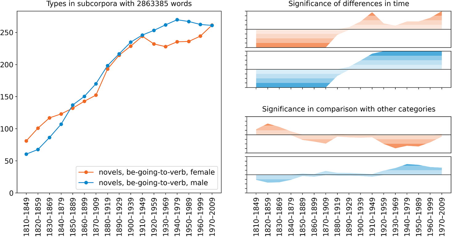
Figure 3. Gender variation and change in the type frequency of be going to V by the number of running words in COHA novels

4.1.6. Focus on diversity

Figures 2 and 3 consider the number of types in terms of the number of running words in the corpus. As noted by Säily (2011: 148), this in essence conflates two measures: how often and how diversely the construction is used. If we want to focus our attention on diversity alone, we can assess the number of different verb types that we encounter in terms of the number of instances (tokens) of the construction: when the construction is used, how diversely is it used? This perspective is presented in figure 4. Interestingly, by this measure the productivity of the construction displays no increase whatsoever over time. In fact, the productivity becomes significantly low in the early twentieth century compared to the corpus as a whole.

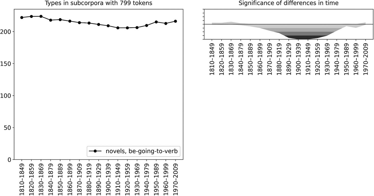
Figure 4. Change in the type frequency of be going to V by the number of tokens of the construction in COHA novels

Figure 5 shows the situation by gender, and this time there is a consistent gender difference: men tend to use the construction more productively than women throughout the two centuries. While the trend view indicates that this difference decreases over time, there are still significant gender differences in periods representing the late twentieth century. This is probably because we have more data from these periods, which enables us to reject the null hypothesis with more certainty, even if the difference might not be as large. When we consider hapax legomena rather than types, the trend remains similar, indicating that male and female authors differ not only in their extent of use of different verbs in the construction but also in what Baayen (2009: 902) calls potential productivity, which estimates the construction’s potential for expansion to new verbs.

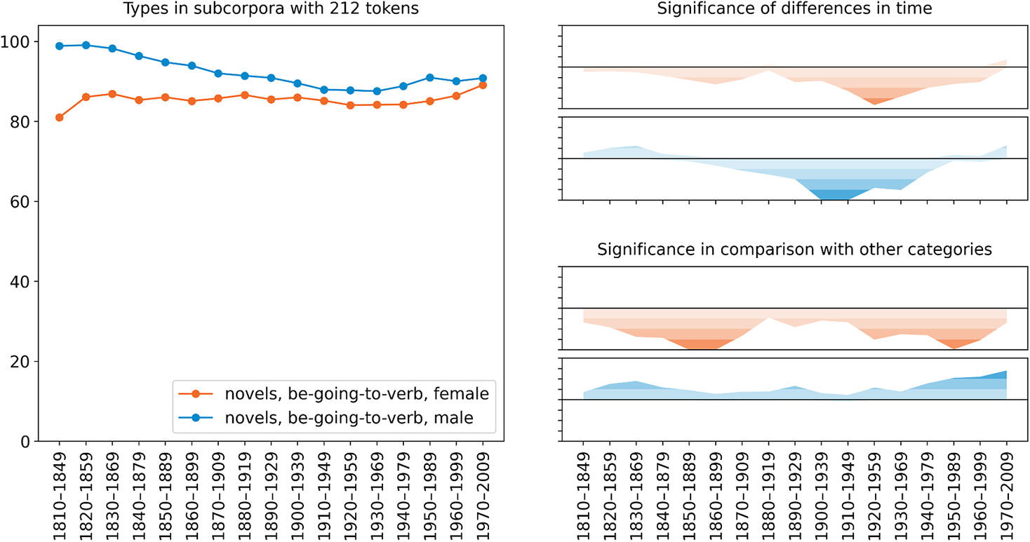
Figure 5. Gender variation and change in the type frequency of be going to V by the number of tokens of the construction in COHA novels

4.1.7. Internal factors

Let us next move on to the internal factors, which paint a rather different picture of variation and change in the productivity of the construction. Here we analyse the proportion of verb types representing the factor in question out of all verb types used in the construction. Firstly, the proportion of mental verb types out of all verb types in the construction shows an increasing trend over time, which is supported by the proportion being significantly low in the initial periods, particularly 1830–69 (figure 6). Moreover, the change is clearly led by women, which is the opposite of what we saw in the overall type frequency. While the gender difference is not very significant, it is quite consistent, which speaks for its being a real phenomenon in the corpus.

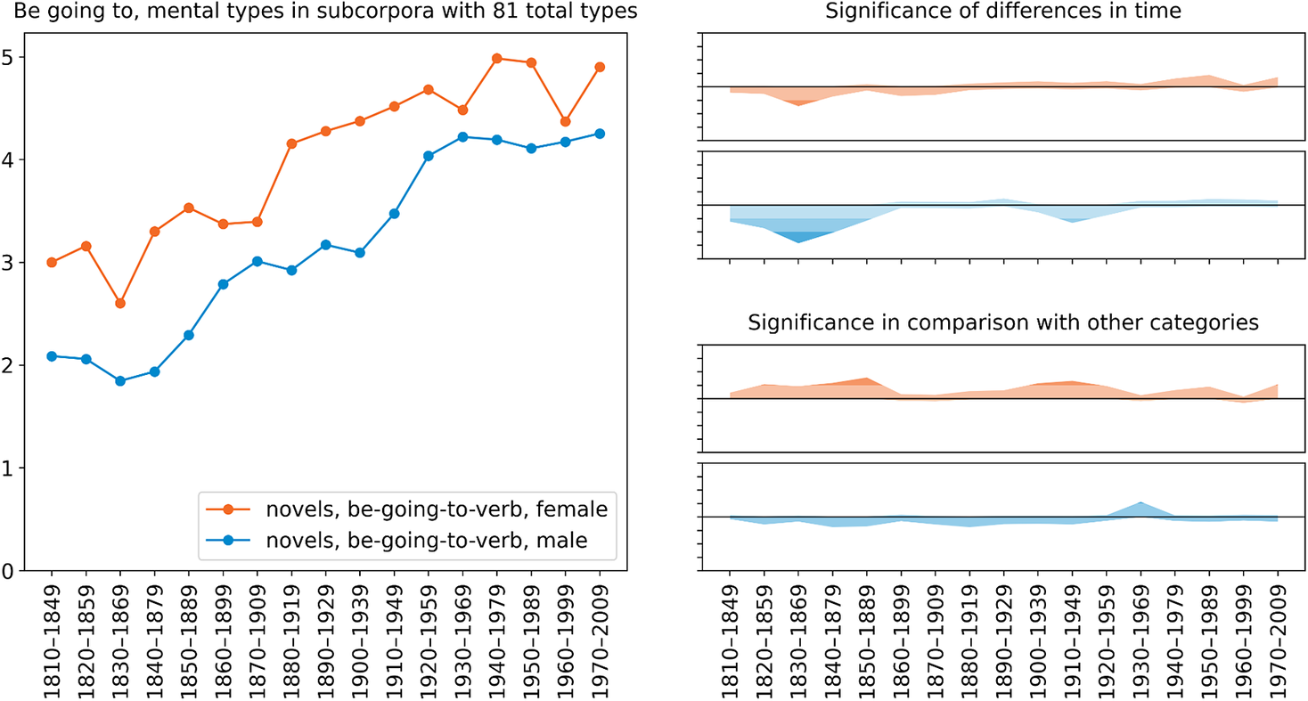
Figure 6. Gender variation and change in the proportion of mental verb types in the be going to V construction in COHA novels

The proportion of verb types used with the inanimate subject it behaves in a similar manner (figure 7). There is an increasing trend over time, and the process appears to be female-led, although this is somewhat less clear in the trend line than in the case of mental verbs. Both of these internal factors indicate increasing productivity of the ‘prediction’ sense of the construction, as in examples (4) and (5) in section 2 above.

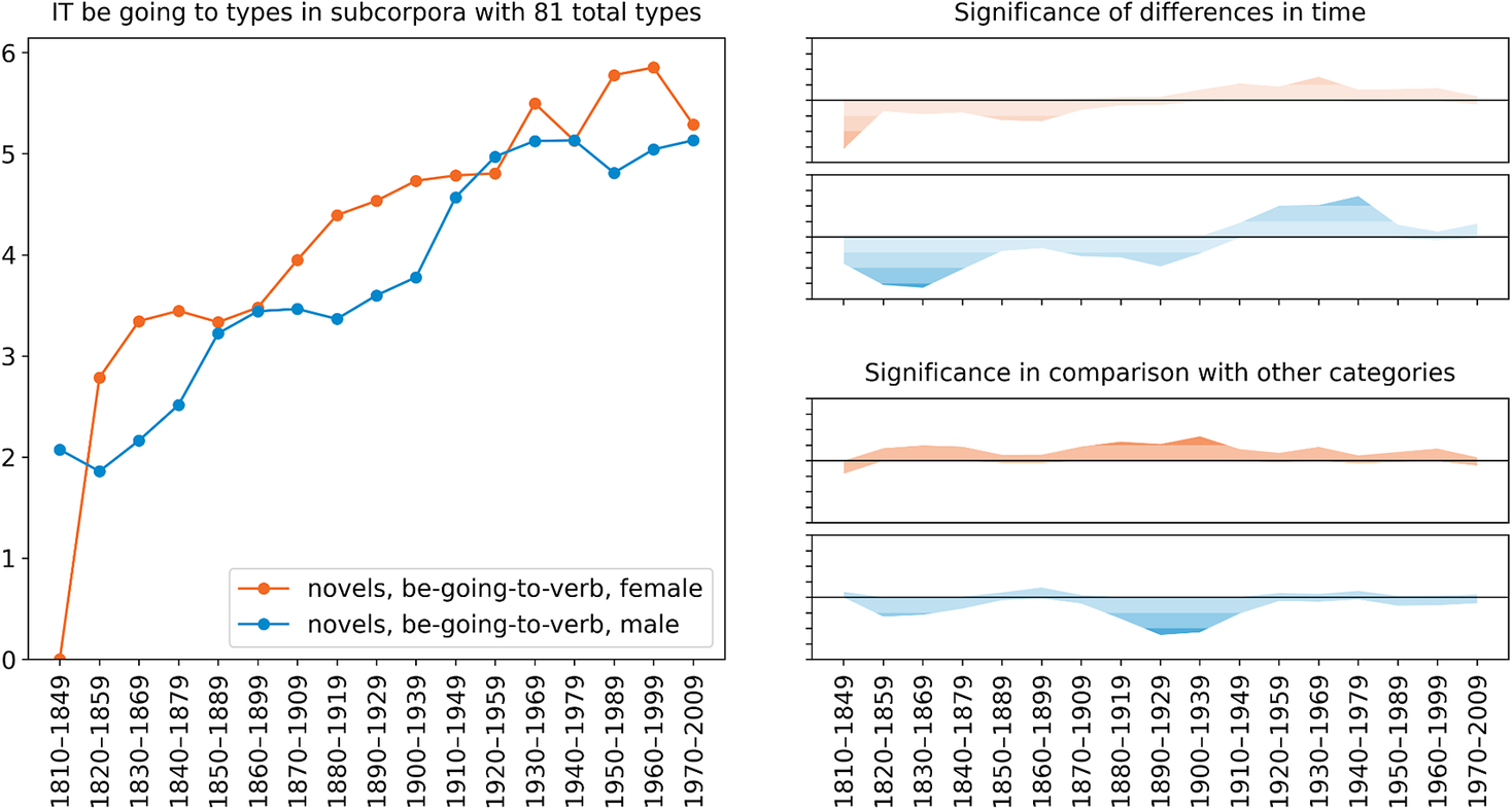
Figure 7. Gender variation and change in the proportion of verb types used with the inanimate subject it in the be going to V construction in COHA novels

Figures 8 and 9 focus on the proportion of verb types used with passive voice (the be-passive) in the construction, as in example (6). The latter figure indicates that overall, the proportion increases over time, peaking around 1930–69. Figure 8 displays no consistent gender difference, although women’s usage is somewhat high in the late nineteenth to the early twentieth century (1870–1909, 1880–1929 and 1890–1939). Furthermore, it is only men for whom we see an increasing trend over time, excepting the first few decades. Women seem rather to have a decreasing trend, but this is not supported by the significance analysis.

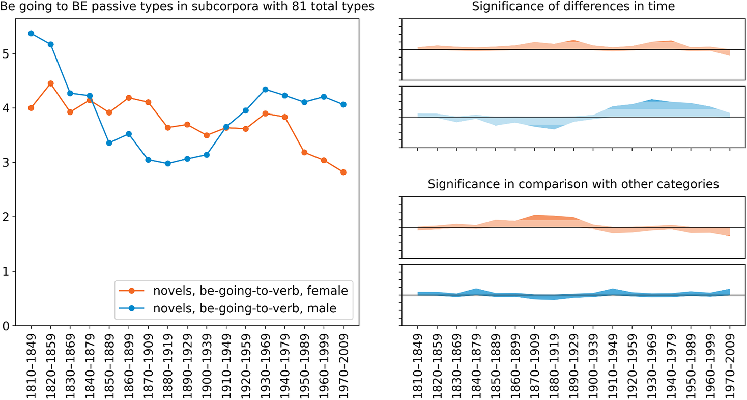
Figure 8. Gender variation and change in the proportion of verb types used with passive voice in the be going to V construction in COHA novels

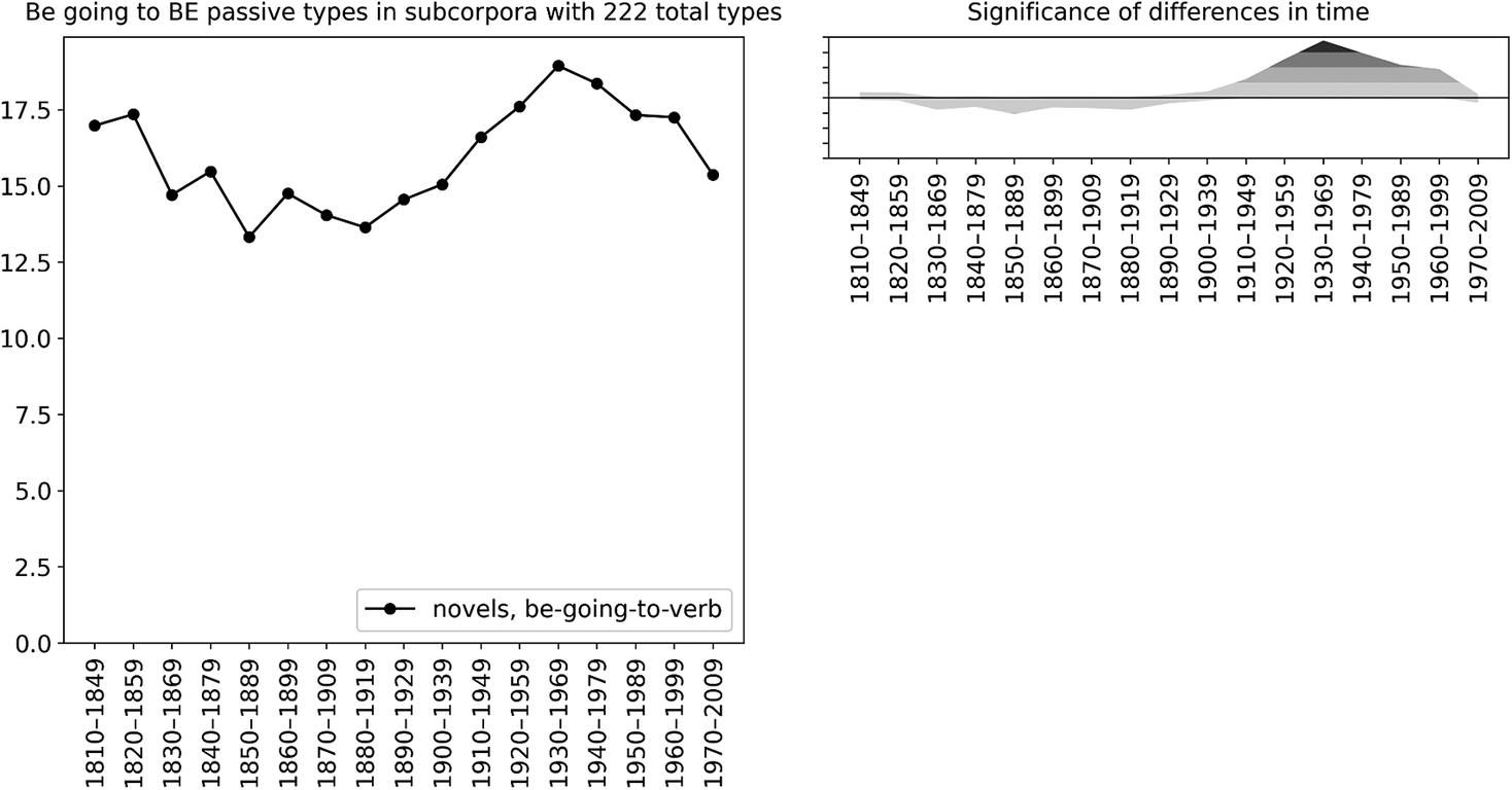
Figure 9. Change in the proportion of verb types used with passive voice in the be going to V construction in COHA novels

4.2. Distributional semantic analysis

Our analysis of the be going to V construction so far has enabled us to identify quantitative differences between female and male writers in their use of the construction. In particular, we detected differences in the type frequency of the verb slot, which is traditionally considered to provide an indication of the degree of openness of a slot. However, a growing number of studies suggest that it is also important to consider what kind of types are in the distribution of a construction. For instance, Suttle & Goldberg (2011) argue that it is primarily variability, i.e. the diversity in the types attested with a construction, that drives the productivity of constructions. The underlying intuition is that some constructions might be restricted to only certain specific semantic areas and others might be compatible with a wide range of meanings, but these differences may not be reflected in type frequency counts.

Against this backdrop, in this section we explore the semantics of the items used in the verb slot of the be going to V construction, and we examine changes to the semantic areas occupied by the construction. In particular, we seek to gauge to what extent the construction becomes increasingly used with verbs that do not align with the ‘motion with purpose’ source of the constructions, and whether this differs between men and women. In this, we expand on the study of mental verbs reported in the last section (see also Wu et al. 2016) by looking at a wider range of semantic areas, and we do so in a more data-driven way. To achieve this, we follow Perek (2016, 2018) and Hilpert & Perek (2022) in adopting a distributional approach to lexical semantics for the study of syntactic productivity. We use distributional semantic representations to measure the semantic spread of the construction over time and between genders.

4.2.1. Distributional semantic model

Distributional semantics is an approach to lexical semantics that aims to capture the meaning of words through their lexical collocates in large text corpora, following Firth’s (1957: 11) oft-cited intuition that ‘you shall know a word by the company it keeps’. It is based on the idea that semantically similar words are expected to have the same collocates. For instance, the verbs drink and sip refer to similar actions (ingestion of fluids), and therefore are expected to co-occur with the same set of words, for instance words for beverages (wine, water, coffee, beer), containers (cup, glass, bottle), as well as words related to drinking or dining practices (restaurant, bar, table, party, etc.). In distributional semantics, words are considered similar in meaning to the extent that they are similar in distribution. In a Distributional Semantic Model (hereafter DSM), the meaning of each word is typically captured as a vector, i.e. an array of numerical values, from which various kinds of quantitative information can be derived. In particular, the semantic similarity between words can be measured by quantifying the similarity between vectors; studies in the field typically achieve this by means of the cosine similarity measure, i.e. the cosine of the angle between two vectors, which thus captures the extent to which two vectors ‘point’ in the same direction in the hyper-dimensional semantic space (cf. Turney & Pantel 2010). The main advantages of the cosine measure are its conceptual simplicity and low computational complexity, and it has been shown to achieve the best results for this purpose over other available measures (cf. Bullinaria & Levy 2007).

For this study, we used a DSM from Perek (2022) created with word2vec, a computational approach to distributional semantics that aims to quantify the relation between a word and its contexts of occurrence in a corpus by means of a neural network (Mikolov et al. 2013); the semantic vectors are derived from the weights of nodes in the layers of the neural network. This model was trained on a PoS-tagged version of the whole COHA corpus; as such, it provides a kind of ‘historical average’ of the meaning of words over the time span of the corpus. While we would ideally need to use different models trained on different sections of the corpus to account for possible lexical semantic change, using a single model means that we use the maximum amount of data for each word, leading to more robust and reliable semantic representations, and it also presents the advantage of facilitating comparisons between periods, since the location of words with respect to each other in the semantic space is held constant. New meanings of verbs have obviously appeared over the past 200 years, but given the relatively shallow time depth and the advanced stage of standardization in English over the period of interest, we can be reasonably confident that the overall meaning of most verbs in our sample has not changed dramatically and that the ‘historical average’ approach should not substantially distort our findings.

The DSM was created with the SkipGram algorithm of word2vec using 1000 dimensions. Given a word, SkipGram attempts to predict its context of occurrence, defined here as the surrounding words in a two-word window (i.e. two words to the left and two words to the right); words are considered similar to the extent that they predict similar contexts. Using the lemma annotations of the corpus, all forms of verbs were grouped together as one word in the model; in other words, each verb was assigned a single vector corresponding to the distribution of all forms of the verb taken together.

4.2.2. Measuring the semantic range of constructions

The method pioneered by Perek (2016, 2018) consists in extracting from a DSM pairwise cosine similarity scores between verbs occurring in a construction at different points in time, and using this information to plot these verbs in two dimensions with multidimensional scaling or t-SNE (Van der Maaten & Hinton 2008). These distributional semantic plots are used to visualize the semantic space populated by these verbs and identify semantically coherent classes of verbs in different time periods, thus showing how the semantic spread of a construction changes over time. However, in its original form, this way of assessing the productivity of constructions suffers from the same issues as measuring type frequency, as discussed in section 4.1.1: since the number of types does not vary linearly with sample size, we cannot compare semantic plots of types found in samples of different sizes, as we cannot be sure that the presence or absence of certain types can genuinely be interpreted as differences in productivity or is simply due to differences in sample size. A possible solution to this issue is to randomly select tokens of the construction so as to match sample size for every time period. For instance, Perek (2018) normalizes samples of the way-construction in the entire COHA corpus by randomly selecting texts from each decade in the corpus so that the set of texts for each decade matches the size of the smallest decade in the entire corpus. The tokens of the construction and thus the corresponding types to be used for the distributional semantic plots are then extracted from the selected texts. However, this approach is only appropriate when the corpus is not too imbalanced, i.e. there is relatively little variation between samples, and in particular the difference in size between the smallest sample and the other samples is not too great. Unfortunately, neither of these conditions are met by the gender-annotated COHA corpus of novels we are using in this study, as described in section 3. Hence, a different approach is needed.

In this study, we adapted the general logic of types3 to the study of the semantic range of a construction in diachrony. In the previous work cited above, semantic change in a construction was assessed by considering individual types and how they relate to the rest of the distribution, but such a qualitative assessment is not possible over randomly selected samples, as specific types may vary widely from one sample to the next, and the range of individual types cannot be straightforwardly averaged over samples in the same way that overall type frequency is in types3. The solution to this issue that we describe below is to sort the types into discrete semantic categories, and then to calculate average type counts in each category across random samples. The distribution of the average type counts over semantic categories provides a representation of the average ‘semantic spread’ of the construction, which can be used to quantify semantic variation in the construction, both between time periods and between genders (see Hilpert & Perek 2022 for a similar approach).

This approach was implemented as follows; all the steps in this procedure were done in R. We used the same dataset as in the types3 analysis presented above. From this data, we extracted randomly selected samples containing the same number of tokens of the construction. We repeated this random sampling 1,000 times for each time period and each gender. To maximize the number of tokens in each sample, we use forty-year periods from 1820 to 1979, hence 1820–59, 1860–99, 1900–39 and 1940–79; changes happening in the three decades after 1979 are thus ignored. The number of tokens in each random sample is set to match the minimum sample size found in our dataset across the whole periodization, i.e. 534 (corresponding to the number of tokens contributed by female writers in the 1820–59 period). As in types3, to preserve the textual units of the corpus, we sample tokens from the same text together.

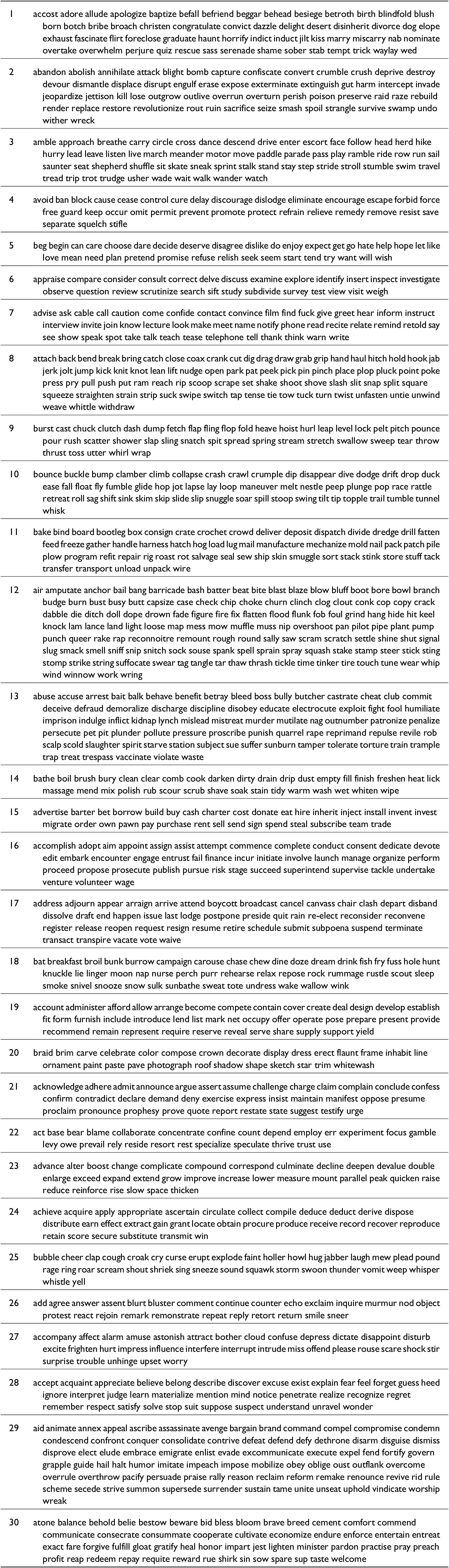
We collected all the types attested in these random samples. We then extracted pairwise semantic similarity scores (using the cosine measure) between these 1,419 types from the DSM described above, and we used these scores to automatically group types into semantic categories using cluster analysis, using the Partitioning Around Medoids (PAM) algorithm from the ‘cluster’ R package. This allowed us to identify semantic classes automatically in a data-driven way, without assuming any prior categorization.

As a variant of k-means, PAM requires the user to specify a target number of clusters when running the algorithm. The ‘right’ number of clusters is typically chosen by comparing different clustering solutions with different numbers of clusters, and deciding which one is most appropriate; our criteria for appropriateness were mostly qualitative. ¹⁰ For our present purposes, we need to divide the verbs into clusters that are large enough for us to measure changes in type frequency, and at the same time are still semantically coherent, i.e. we are able to assign a relatively precise semantic definition that covers most members of each cluster. The total number of clusters should also not be too high, so that we are able to examine change in each cluster individually and compare it to other clusters. We tried clustering solutions of increasing numbers of clusters (namely, 10, 20, 30 and 40) and checked each solution qualitatively for these criteria. We found a thirty-cluster solution to strike a good balance between a reasonably low number of clusters that at the same time were still largely semantically coherent. This number was also low enough to enable individual analysis. The full list of clusters with all their verbs can be found in the appendix.

For each of the thirty clusters of verbs thus identified, we calculated the average number of types attested in each period and for each gender across the 1,000 samples. For instance, sample 1 contains two types belonging to cluster 1 in period 1 (1820–59) for men, sample 2 two types as well, sample 3 four types, etc., and when we average over all the samples, we find a mean of 2.824 types in period 1 for men. The outcome of this procedure is two matrixes of average type counts per time period and per cluster, one for men and one for women. Because the total average type counts vary slightly from one period to the next, as a final step we converted the average type counts into type proportions, by dividing the type count of each cluster by the total type count of the relevant time period. This provides an indication of the prominence of each semantic class within the distribution of the construction. Two types of analysis can be applied to this data: (i) a general quantitative analysis comparing the distribution of the construction between periods and between genders, i.e. the columns of the matrixes, and (ii) a fine-grained, more qualitative analysis focusing on particular semantic classes and measuring type frequency variation in these classes for each gender. We present each type of analysis in turn.

4.2.3. Overall results

Tables 2 and 3 report similarity scores between the type distributions of the construction for different periods or genders as measured by Pearson’s correlation coefficient (ρ). Pearson’s ρ measures correlations between vectors and varies between -1 and 1, with -1 indicating a negative correlation, 1 a positive correlation, and 0 no correlation; hence, the closer to 1 ρ is, the more similar the two distributions are. Table 2 reports comparisons between adjacent periods, for men and for women; in this table, a lower ρ indicates change over time, and a higher ρ indicates stability. Table 3 reports comparisons between genders in the same period; in this case, a lower ρ indicates divergence, and a higher ρ indicates similarity in usage.

Table 2. Change in the semantic distribution of be going to V for each gender, as measured by Pearson’s ρ

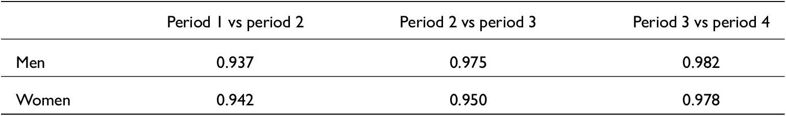
Table 3. Comparison of the semantic distribution of be going to V between genders over time, as measured by Pearson’s ρ

Table 2 shows that change is happening in the distribution of the construction from period 1 to period 2 to a similar extent for both genders, although the degree of change is arguably very modest, as ρ is over 0.9. This lines up with the finding that, by the early nineteenth century, the be going to V construction has fully acquired its modern meaning (though not its full Present-Day English distribution) and is thus already open to a very wide range of verbs, leaving few semantic areas that have not yet been covered. At the same time, the amount of change decreases over time (i.e. ρ increases), especially for men, as distributions become more similar from one period to the next. Table 3 shows that the way men and women use the be going to V construction is already very similar from the first period on, but it becomes even more similar throughout the nineteenth and early twentieth centuries, which indicates that the two genders are converging in their use of the construction.

Figure 10 focuses on each of the thirty semantic classes individually, as it plots the variation in type count proportions in each class over time separately, for men (blue) and women (red). This allows us to identify which classes show gender differences in productivity, i.e. cases in which one gender uses more types in one class than the other gender at a given point in time.

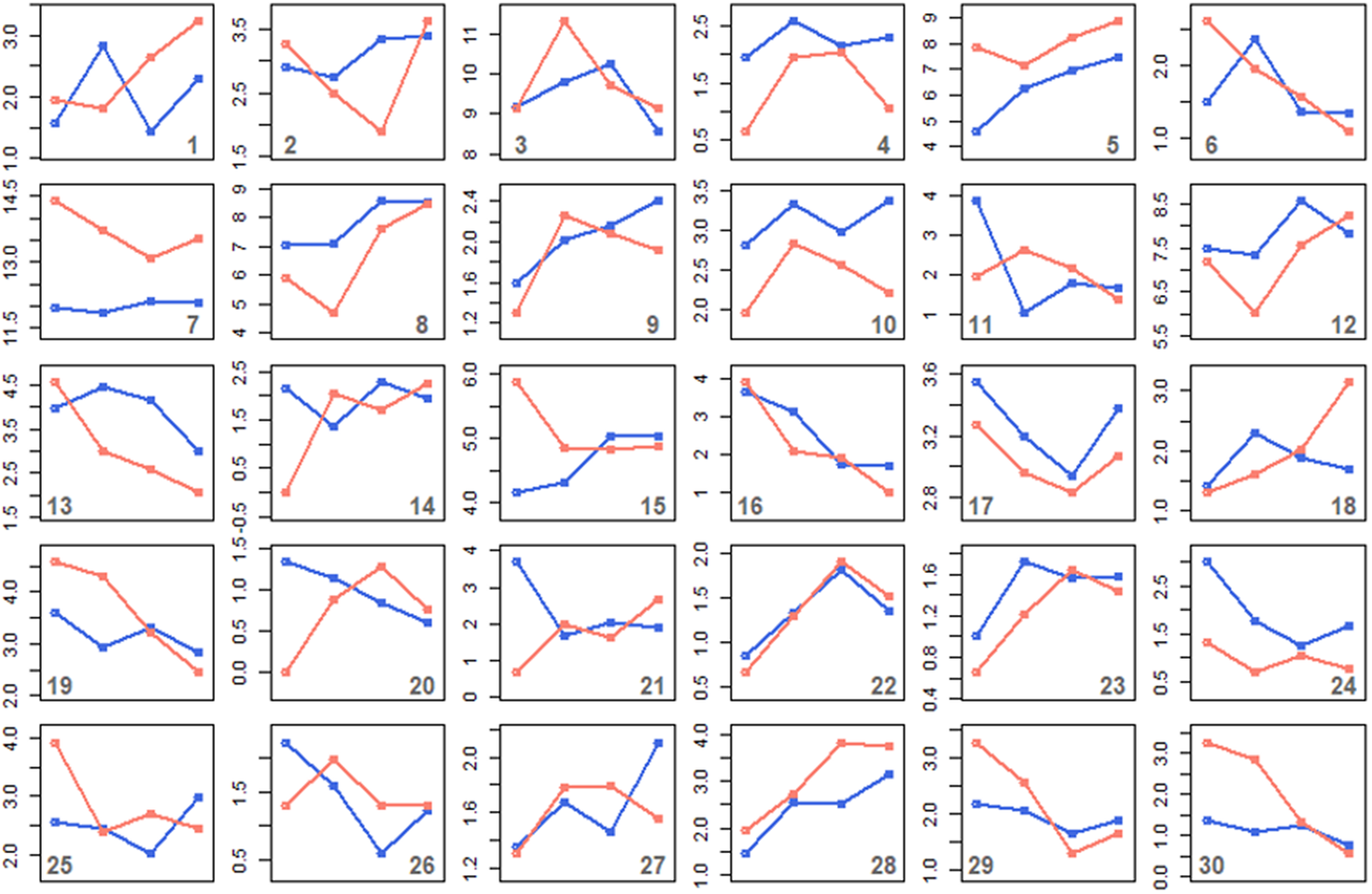
Figure 10. Variation in type proportions in each class over time, for men (blue) vs women (red). Samples are taken from four periods: 1820–59, 1860–99, 1900–39, 1940–79

As can be seen in figure 10, while in some classes the type proportions are roughly similar between genders and follow the same trends (e.g. clusters 9, 16, 22), many others do show some gender differences. It is beyond the scope of this case study to discuss each of them in detail, and another reason why it might be difficult to do so anyway is that, while many of the clusters can indeed be interpreted semantically and can clearly be assigned to a particular semantic class of verbs, not all of them can; some correspond to a collection of various classes rather than a single coherent semantic category. Such an outcome is not unexpected given the low number of clusters and the high number of verbs, but it makes it difficult to interpret changes in type frequency for such heterogeneous classes. Therefore, we will only focus on a small selection of classes that do receive a clear semantic interpretation, but this should not be taken as an exhaustive representation of the changes happening to the distribution of the construction.

4.2.4. Analysis of individual semantic classes

Table 4 lists the six clusters chosen for the analysis, which we discuss in turn below. In each cluster, most verbs can be seen to correspond to a broad semantic class, identified in the first column, although there are also some outliers, listed in brackets below the main group. In some cases, even the outliers can be seen to relate somehow to the meaning of the group, for instance many of the outliers to the sound emission verbs (cluster 25) do refer to events that typically involve some sound, e.g. clap.

Table 4. Semantic clusters of verbs chosen for the analysis

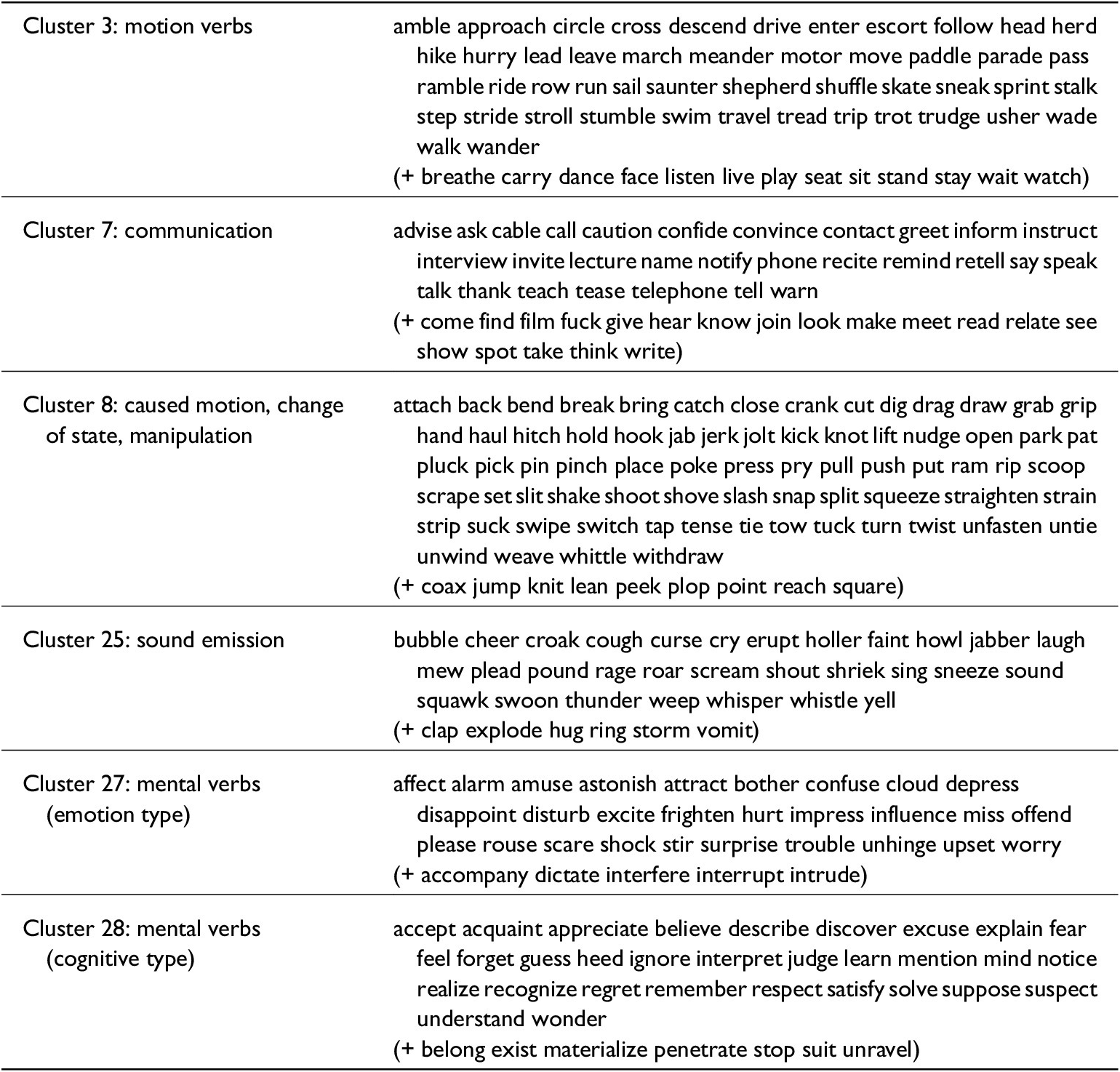
First, cluster 3 contains verbs of motion, including many verbs encoding manner of motion, e.g. amble, meander, sneak, run, as exemplified by (7) and (8). We would argue that such a group is especially relevant to the study of the productivity of be going to V, given the semantic source of the construction. In the original ‘motion with purpose’ meaning of be going to V, it would seem incongruent to make the purpose of motion another form of motion: one does not normally go somewhere in order to go somewhere else. Hence, occurrence of verbs of motion in the construction can be seen as a sign that it has grammaticalized into its futurity meaning (cf. Traugott & Trousdale 2013: 118), and increased productivity in this class indicates a weakening of lexical persistence effects and further abstraction of the constructional meaning. As seen in figure 10, women seem to be ahead of men in using this class productively in the middle of the nineteenth century, though men quickly catch up in the twentieth century. If we examine this cluster of verbs in types3 by looking at the proportion of cluster 3 types out of all verb types in the construction over time, we obtain very similar results. This can be taken to suggest that the construction initially shows a higher degree of grammaticalization for female writers than for male writers, at least with respect to this class.

Similar comments can be made in relation to cluster 27 and cluster 28. Both clusters correspond to a general class of mental verbs, and indeed many verbs from Halliday & Matthiessen’s (2014: 256–7) list are found in them. The two clusters can be distinguished in that the former mostly corresponds to what Halliday & Matthiessen term the emotion type (e.g. fear, impress, shock), and the latter mostly corresponds to the cognitive type (e.g. believe, suspect, understand), as exemplified by (9) and (10) respectively. As argued above, these verbs too are relevant to the grammaticalization of be going to V, as they are predicates that are a priori not tied to spatial location, and thus the ‘motion with purpose’ source meaning of the construction is not readily compatible with them. Women seem to be slightly more productive with these verbs than men, albeit in different ways. In the emotion type, women are ahead in periods 2 and 3 (i.e. from 1860 to 1939), but they are overtaken by men in the mid twentieth century. In the cognitive type, the female preference is initially quite small, but women are consistently in the lead, and the gap between men and women markedly widens after 1940, with women using the cognitive type much more productively. These findings roughly follow the same trends as the analysis using the types3 software reported in section 4.1.7, but they also suggest that not all mental verbs behave in exactly the same way, which shows the benefits of the distributional semantic approach in identifying verb classes. It is not clear how the difference between these two groups should be explained, but it could be related to the fact that women also seem to be ahead of men in using the construction with an inanimate subject, as reported earlier (see figure 7): most verbs in the emotion group take a stimulus argument as subject that can be inanimate, and thus are more likely to have an inanimate subject than the verbs in the cognitive group, which predominantly take an animate experiencer as subject.

Cluster 7 and cluster 25 exemplify two related domains: the former contains communication verbs (e.g. ask, talk, warn), the latter includes some manner of speaking verbs (e.g. whisper, yell) as well as various verbs conveying sound emission, which can often be used in a communication or social interaction sense (e.g. croak, laugh, roar, scream); see examples (11) through (13). Interpreting these verbs with respect to the degree of grammaticalization of the construction is less straightforward than with the classes discussed so far, but since many of these verbs are of a relatively abstract type and their meaning is not necessarily tied to spatial location, it is fair to assume that they at least occupy an intermediate position between verbs that lend themselves well to the ‘motion with purpose’ interpretation, and verbs that are incompatible with it. Although the general diachronic trend in both classes is one of decline relative to other classes, women seem to use both classes markedly more productively than men, at all times for verbs of communication, and only up until the twentieth century for verbs of sound emission.

Women seem to show a higher degree of productivity in the classes discussed so far, but this is not always the case, and in some clusters it is men who are in the lead. A particularly good example of this is cluster 8, a diverse class of loosely related items which are unified by a high degree of physicality: verbs of caused motion (e.g. bring, place, pull), change of state verbs (e.g. break, cut, open), and verbs of forceful contact and manipulation (e.g. attach, kick, squeeze). Men consistently use this class more productively than women up until the mid twentieth century. With regards to the grammaticalization of the construction, these verbs arguably lend themselves more readily to the original ‘motion with purpose’ meaning than the other classes discussed so far, as they are simply more tied to the physical realm. Hence, the productivity of the construction in this class can be interpreted as an effect of lexical persistence, and conversely, it does not suggest a higher degree of grammaticalization of the construction. A possible explanation for the gender difference in this class could thus be that men generally use the construction more conservatively than women, which directly mirrors the more innovative behaviour displayed by women in the classes discussed above.

5. Discussion and conclusion

Our findings indicate that contrary to the results of Wu et al. (2016) on token frequency, the overall type frequency of be going to V does not increase over time in the Late Modern and Present-Day American English of our dataset, and there is even a slight decrease in the early twentieth century. It would then seem that productivity-wise, the grammaticalization process has stalled since the nineteenth century. Moreover, we have found that men’s usage of the construction is more productive than women’s, with a converging trend over time.

However, the situation is reversed when we consider intralinguistic factors related to subjectification: the proportion of mental verb types, verb types used with the inanimate subject it, and verb types used with passive voice in the construction all exhibit an increasing trend over time. Moreover, the first two changes appear to be led by women. Thus, by zooming in on the internal factors, we can see that the ongoing process of subjectification manifests itself not only as increases in token frequency (Wu et al. 2016; Budts & Petré 2016) but also in productivity, and far from stagnating, the grammaticalization process is still ongoing from this perspective. The fact that two out of three of the proportional changes are led by women is in accordance with previous sociolinguistic research (e.g. Labov 2001), and the contrary findings from morphological productivity (e.g. Säily 2014; Säily et al. 2024) are not replicated for syntactic productivity. More research is, however, needed to verify these tendencies regarding different levels of linguistic organization.

Supporting and augmenting the results on mental verb types, our data-driven type-based semantic analysis also identifies areas of growth. These include a cluster involving verbs of motion, which indicates grammaticalization in terms of futurity, as well as two clusters of mental verbs, which roughly map onto Halliday & Matthiessen’s (2014: 256–7) emotive and cognitive categories. The emotion verbs in particular could be linked to the ‘prediction’ sense indicating subjectification. All of these changes appear to be female-led, although male authors catch up in the twentieth century first in terms of motion and then emotion.

If we assume that the fiction data used in this study is a faithful reflection of men and women’s knowledge and usage of the construction, in a DCxG account our results would suggest slightly different representations of the construction over time for these two groups of speakers. Both the higher prominence of inanimate subjects and the higher diversity of verbs in particular semantic classes (namely mental verbs as well as other narrow classes identified in the distributional semantic analysis) could indicate that the construction is initially slightly more schematic for female authors than male authors (Perek 2020), in that it more readily sanctions uses that are in line with the more general ‘prediction’ sense, but not with the more narrow ‘intention sense’, much less with the original ‘motion with purpose’ meaning of be going to V. More research is certainly needed to confirm this interpretation, for instance by including a wider range of internal factors.

We have seen that at the stage of grammaticalization of be going to V displayed by our dataset, the overall type diversity of the construction stagnates but internal factors linked to grammaticalization indicate increasing productivity. This implies that internal factors are important to account for in analyses of productivity. Furthermore, we have found consistent gender differences in our dataset. While many of the changes seem to be female-led, there is a caveat here: male and female authors may tend to write in different subgenres of novels, which could influence the results. For instance, if women wrote more in genres characterized by a personally involved style, they would have more occasion to utilize mental verbs in general. When comparing the overall token frequencies of these verbs by gender, however, we observed no consistent correlation with their usage within the construction. Therefore, gender cannot be ignored as a possible factor, and many diachronic constructional analyses would benefit from considering it (cf. Säily et al. 2024).