Impact of increased anthropogenic Amazon wildfires on Antarctic Sea ice melt via albedo reduction

Abstract

This study shows the impact of black carbon (BC) aerosol atmospheric rivers (AAR) on the Antarctic Sea ice retreat. We detect that a higher number of BC AARs arrived in the Antarctic region due to increased anthropogenic wildfire activities in 2019 in the Amazon compared to 2018. Our analyses suggest that the BC AARs led to a reduction in the sea ice albedo, increased the amount of sunlight absorbed at the surface, and a significant reduction of sea ice over the Weddell, Ross Sea (Ross), and Indian Ocean (IO) regions in 2019. The Weddell region experienced the largest amount of sea ice retreat ($ \sim \mathrm{33,000} $ km²) during the presence of BC AARs as compared to $ \sim \mathrm{13,000} $ km² during non-BC days. We used a suite of data science techniques, including random forest, elastic net regression, matrix profile, canonical correlations, and causal discovery analyses, to discover the effects and validate them. Random forest, elastic net regression, and causal discovery analyses show that the shortwave upward radiative flux or the reflected sunlight, temperature, and longwave upward energy from the earth are the most important features that affect sea ice extent. Canonical correlation analysis confirms that aerosol optical depth is negatively correlated with albedo, positively correlated with shortwave energy absorbed at the surface, and negatively correlated with Sea Ice Extent. The relationship is stronger in 2019 than in 2018. This study also employs the matrix profile and convolution operation of the Convolution Neural Network (CNN) to detect anomalous events in sea ice loss. These methods show that a higher amount of anomalous melting events were detected over the Weddell and Ross regions.

Impact Statement

Sea ice protects ice sheets, which are melting at a very high rate to raise the sea level. In addition to global warming, this study is indicative that black carbon aerosols transported from anthropogenic wildfire events, such as from the Amazon, darken the snow, reduce their reflectance, increase the absorption of solar energy incident on the surface, and exacerbate the sea ice retreat. Thus, this study points out that anthropogenic wildfire impacts far away from a region can have a severe impact on sea ice and ice sheets over the Antarctic which has a sea level rise potential of 60 m. Our study shows that only over the Weddell region, sea ice retreat was 20,000 $ {km}^2 $ higher during the presence of BC transport events than other days in 2019.

1. Introduction

With $ \sim 60\% $ of the global population living within 100 km of a sea or oceanic coast Barragán and De Andrés (2015), the melting of ice sheets over the Antarctic has raised a concern among the scientific community. Ice sheets in the Antarctic region are losing ice mass ( $ \sim 146 $ Gt per year) at a much lower rate than the Arctic region ( $ \sim 250 $ Gt per year) Nasa Climate Change (Accessed: Feb. 26, 2024). This can be attributed to the vast sea ice over the Southern Ocean that was able to maintain its extent Nsidc Sea Ice Matters (Accessed: Feb. 26, 2024) till 2014 with a record winter high extent noticed in 2010 Parkinson (2014). The presence of vast sea ice cover over the Southern Ocean provides a thermal buffer to the ice sheets on land as well as the floating portion of the ice sheets and dampens the wave and wind action Nsidc Sea Ice Matters (Accessed: Feb. 26, 2024). Unfortunately, the Antarctic Sea ice is now retreating faster and has reached a new record low of 1.965 million $ {km}^2 $ in 2023 ( $ \sim 32\% $ below climatological values) Raphael and Handcock (2022). The ice sheet melt has accelerated in recent times as the Antarctic region has lost $ \sim 300,\sim 575, $ and $ \sim 250 $ Gt of ice in 2019, 2020, and 2021, respectively, Nasa Climate Change (Accessed: Feb. 26, 2024). This is important to note that the Antarctic ice has the potential of sea level rise by 60 m as compared to Greenland, which has a sea level rise potential of 7 m. Thus, the recent acceleration in sea ice as well as ice sheet melting is of great concern to the human community and ecosystem.

It is still not known what the reason behind the recent retreat of sea ice and the acceleration of the ice sheet melting over Antarctica is. So far, most of the studies and tools have focused on the ice sheet melting and sea level rise due to the $ {CO}_2 $ concentration and global temperature rise based on various measurements from different observational sources and different Shared Socioeconomic Pathways (SSP) and the Representative Concentration Pathways (RCP) scenarios Tamura et al. (2019); Rohmer et al. (2021); Nasa Sea Level Tool (Accessed: Feb. 26, 2024); Sea Level Rise Projections (Accessed: Feb. 26, 2024). When sea ice melts, darker-colored liquid water is left exposed to absorb sunlight. As the snow albedo (a measure of light reflection) decreases, the amount of reflected sunlight to the space decreases, a higher amount of incident sunlight is absorbed at the surface, and leads to sea ice melting Tamura et al. (2019).

Incidentally, this period of accelerated ice sheet melting and vanishing sea ice extent coincides with the rapid increases in the slash-and-burn practices over the Amazon rainforest between 2018 and 2022 Escobar (2019). Wildfires generate several Black Carbon (BC) particles that are capable of absorbing solar energy and darkening the snow Hansen and Nazarenko (2004); Flanner et al. (2007). Snow darkening by black carbon (BC) aerosols significantly amplifies the greenhouse effect by two times and accelerates ice sheet melting Hansen and Nazarenko (2004) because they absorb sunlight, warm the surface where they deposit, and darken the snow and ice surface Hansen and Nazarenko (2004); RFASAC (Accessed: Feb. 26, 2024). The satellite era shows that aerosol atmospheric rivers (AAR), long and elongated channels of strong wind and extreme mass transport, can transport these aerosols to long distances—often intercontinental Chakraborty et al. (2022, 2021). A reduction in ice albedo diminishes the reflection and steers towards a higher absorption of the incoming solar energy, increases the surface temperature, accelerates the melting process, and further reduces albedo—leading to a positive feedback loop Hansen and Nazarenko (2004); Flanner et al. (2007). In 2019, the Amazon rainforest witnessed the worst-ever deforestation and man-made wildfire events Escobar (2019) for agricultural purposes Lovejoy and Nobre (2019). Owing to such an acceleration of the sea ice melting, it is of primary importance to investigate if the Antarctic Sea ice is vulnerable to forest fire-generated aerosols from the Amazon. If the aerosol deposition over the sea ice has exacerbated the ongoing sea ice melting due to global warming, it is of utmost importance for the climate community to focus on the imminent threat of Amazon wildfires not only on the sea ice but also on the land ice melting over the Antarctic region.

This article takes advantage of the multiyear remote sensing measurements from various satellites (Table 1) over the Antarctic region (60° S–90° S; 180° W–180° E). We use various measurements of radiative properties, precipitation, humidity, and AAR, aerosol optical depth to infer the plausible reasons for the extreme sea ice melt. In this study, we estimate the change in the sea ice extent (SIE) over the Antarctic. The sea ice extent data has been obtained from the National Snow and Ice Data Center. The sea ice extent data has been obtained from various sensors (Table 1) and has been extensively used to study sea ice changes Fetterer et al. (2002); Diebold et al. (2021); Fetterer and Knowles (2004). We employ various machine learning and anomaly detection techniques that can model spatial and temporal processes such as McGuire et al. (2008); Janeja and Atluri (2005); Walkikar et al. (2024); McGuire et al. (2014); Chandola et al. (2009) to understand the role of aerosols on the exacerbated sea ice loss in terms of their extent in $ {km}^2 $ , such as random forest, elastic net regression, convolutional operation of CNN, and matrix profile analyses that are described in detail in the methodology section. The choice of machine learning techniques has been adopted based on their usefulness for this particular kind of study and the previous studies that have successfully implemented these techniques to study and address various climate change-related problems Gaál et al. (2012); Guyennon et al. (2021); Zhai et al. (2023); Chakraborty et al. (2015); El Khansa et al. (2022).

Table 1. Satellites and list of the parameters used with acronyms and units

Note. All the datasets are between 2018 and 2020 and have been preprocessed at $ 0.25{}^{\circ} $ resolution at a daily scale.

Table 2. Longitudinal range for five regions in different Antarctic regions

2. Datasets

See Table 1.

3. Methodology

3.1. Data preprocessing and domain

While satellite data is immensely helpful for this study, datasets from various sensors onboard multiple satellites have different temporal resolutions. For example, the IMERG data from the Global Precipitation Measurement Mission, which provides information about global precipitation, has a resolution of $ 0.1{}^{\circ} $ . In contrast, the global cloud cover measured by the CERES satellite onboard NASA’s A-train constellation has a resolution of $ 1{}^{\circ} $ . This poses a significant hindrance in data analysis for the scientific community, including data scientists. Owing to the different resolutions of the datasets used in this study (Table 1), we converted all the datasets to $ 0.25{}^{\circ} $ .

Python xESMF is a powerful and popular package that is often used for re-gridding Zhuang (2023); Ali and Wang (2022); Ali et al. (2022) various datasets used in climate change-related studies from sea ice prediction to weather forecasting Ali and Wang (2022); Rasp et al. (2020). Moreover, it is often used to re-grid various data formats, especially the netCDF format Wilson and Artioli (2023) which is often used to store satellite datasets. The package can handle both curvilinear and rectilinear grids, allowing datasets to be re-gridded between any grid types, such as from curvilinear to rectilinear or vice versa. The package has been successfully implemented for Lagrangian as well as Eulerian interpolations Jiang et al. (2023) for the oceanic datasets from various climate simulations The package gained so much popularity that a study shows that events like weather forecasting using data Rasp et al. (2020) can be used after re-gridding using the Python xESMF package. Thus, this study leverages the usefulness of the package to re-grid various datasets available from multiple sensors that have been measured by space agencies like NASA, JAXA, and ESA. After processing the data into a uniform $ 0.25{}^{\circ} $ spatial and daily temporal resolution, thorough and careful checks have been performed to assess if any loss has occurred during processing the data from different resolutions to $ 0.25{}^{\circ} $ over different regions in Antarctica by comparing the datasets between their native resolution and the processed data. Figure 1c and Table 2 summarize the longitudinal range for all five regions in the Antarctic namely the Ross Sea (Ross), the Weddell region (Weddell), the Indian Ocean (IO), the Bell-Amundsen (BA) region, and the Pacific Ocean (PC). Longitudinal interval is assigned to each of the five different polar regions of the Antarctic basin. An $ N\times P $ matrix is created for each region where N represents the number of days with no missing values in each data and P denotes the number of features. Similarly, we have created a matrix of the SIE parameter containing data from N number of days.

Figure 1. Mean and standard errors of SIE loss over different regions in season18 and season19 during BC and non-BC days.

Figure 2. (a) Differences in the number of BC AAR occurrences over the Antarctic region during season19 and season18. (b) same as in (a), but for albedo reduction between season19 and season18, and (c) same as in (a), but for differences in SWD-SWU (solar energy absorbed) between season19 and season18.

It is important to note that the sea ice melt is stronger during the Austral spring and summer. An example is included in Figure 2 showing the SIE between 2018 and 2020 over the Weddell region is prone to sea ice loss. Thus, we focus on the SIE loss from August 2018 to February 2019 (season18) and August 2019–February 2020 (season19) to assess the impact of the BC aerosols transported from the Amazon region. We calculate the differences in the number of AARs arrived, SIE loss, and number of discords in SIE over the region between the two-time frames mentioned above. We also show our interpretation of the possible causes of the SIE loss during 2018–2020 by using random forest, elastic net regression, and causal discovery analysis.

3.2. Matrix profile

In time series analysis (such as Dey et al. (2009); Atluri et al. (2018)), a matrix profile is a data mining tool that quantifies the similarity between various data subsequences in the time series Zhu et al. (2018, 2016). In essence, it represents the shortest distance between each subsequence in the time series and the match that is most similar to it. A subsequence is defined as any segment of the time series that is continuous in nature. For instance, if daily temperature measurements are available for an entire year, the temperatures from January could be a subsequence. Motifs are recurring patterns identified in time series data. The subsequent sequences are exceedingly similar and symbolize frequent patterns of behavior within the dataset. In contrast to motifs, discords consist of subsequences that deviate substantially from one another Barz et al. (2017); Imani and Keogh (2021). For example, unusual melt time periods may be identified as discords.

The discords are discerned by locating the subsequences in the matrix profile that have the highest values, signifying their greatest degree of dissimilarity from the remaining data. In this study, we employed a matrix profile over the sea ice extent variable on each grid cell across Antarctica to obtain the discords. This aids in discovering the regions within Antarctica that experienced high sea ice retreats. This approach effectively identifies irregularities in extensive time series datasets. Interquartile range (IQR) was employed to further distinguish the most exceptional discords. Using the IQR, we determined upper and lower bounds or thresholds used to detect anomalous discords: the upper bounds are the 75th percentile plus 1.5 times the IQR, and the lower bounds are the 25th percentile minus 1.5 times the IQR.

3.3. Causal discovery

This research employed the Partial Correlation-based causal discovery Algorithm (PCMCI +) Runge (2020) as the foundational tool for examining causal connections between various variables within five distinct polar regions in the Antarctic basin. The PCMCI + method is known for its effectiveness in identifying causal relationships in datasets with multiple variables over time. To assess the statistical significance of these causal relationships, we adopted a p-value criterion of 0.05. Recognizing the intrinsic delays in variables’ responses, the research design incorporated time lags of 1, 2, and 3 days. This consideration was crucial for capturing the potential delayed effects among variables, allowing us to account for the temporal dynamics that characterize the Antarctic environment. This approach was carefully designed to examine the complex causal interactions among the variables under investigation, with the sea ice extent variable. Through the application of the PCMCI + algorithm, our objective was to reveal the essential causal mechanisms that influence the interactions among the variables and their consequent impact on sea ice extent, thereby providing insights into the dynamic processes shaping the Antarctic environment.

3.4. Random forest

Random forests are often used in climate studies for various tasks such as climate modeling to identify the most important features when there are a number of predictor variables Gaál et al. (2012); Guyennon et al. (2021); Zhai et al. (2023) as in this study. This can provide valuable insights into the drivers of the target variable and also rank the effects of the features on the target variable. Random forests can be used to predict and analyze the likelihood and severity of these events based on historical climate data and other relevant variables.

3.5. Elastic net regression

Elastic net regression is another machine learning technique largely used in climate studies, particularly in the context of statistical modeling and data analysis Chakraborty et al. (2015). As compared to the traditional multiple linear regression, elastic net regression is a mixed Lasso and Ridge regression technique, which allows it to handle multiple features targeting a predictive variable (here, SIE). It considers the inter-dependency among the features where features can also be correlated with each other. In climate-related studies, features are often related to each other making elastic net regression suitable for such studies. Elastic net regression automatically identifies and gives appropriate coefficients to important features.

3.6. Convolutional operation of CNN

CNN has been used in numerous fields Bouvrie (2006); Paul et al. (2024); Devnath et al. (2023) including classification and prediction of sea ice extent Alzubaidi et al. (2021); Huang et al. (2023); Kareem et al. (2021). Inspired by CNN, our method is based on a recently developed inverse max pooling concept in the convolutional operation of CNN Devnath et al. (2024) to detect anomalies. Our method is developed to offer a solution without using a neural network, and unlike a full CNN, it follows a systematic approach to detect anomalous melting events in a series of RGB satellite images. Initial preprocessing involves converting images to grayscale and creating consecutive grayscale images. The algorithm then calculates difference matrices between successive images, representing spatial and temporal changes, followed by resolution reduction through zero-padding. Statistical analysis of the reshaped array from the reduced resolution matrices list yields essential metrics such as the first quartile (Q1) and the lower bound of the interquartile range ( $ Q1-1.5\times IQR $ ), crucial for defining anomaly criteria.

Specific conditions related to the typical and extreme behaviors of sea ice data are applied, and the algorithm proceeds to identify regions with anomalous melting. This is achieved by comparing mean-pooled and max-pooled (absolute values of the SIE loss) values from the reduced resolution matrix against the expected statistical range and anomaly criteria. An innovative condition, expressed as the ratio of mean-pooled to max-pooled values, is introduced. For each pixel in the reduced resolution matrix, this ratio captures the relationship between the mean behavior and extreme deviations of the sea ice data.

The anomaly detection condition is formulated as follows: if the ratio surpasses a predefined threshold, determined by Q1 and the lower bound of IQR, the corresponding pixel is flagged as exhibiting anomalous melting. The anomalies detected in this process are superimposed onto the original RGB images, offering a visual representation of areas experiencing anomalous melting patterns. This holistic approach, combining statistical metrics, convolutional operations, and pooling techniques, significantly enhances the algorithm’s ability to discern anomalous melting events within the dynamics of Antarctic Sea ice.

We have refrained from employing the training and testing phases of a CNN in our approach. We aim to identify anomalous melting events in satellite images depicting Antarctic Sea ice dynamics. Traditional CNNs are often employed in tasks that involve learning from labeled datasets through training phases, followed by testing on unseen data to evaluate their generalization performance. However, our anomaly detection task is inherently different. We focus on discerning anomalous patterns, regions, and subtle changes in Sea Ice Extent (SIE) from a series of satellite images, where anomalies may not be easily labeled or follow a conventional training/testing paradigm. Anomalous melting events often manifest in diverse and unpredictable ways, making it challenging to establish a comprehensive labeled dataset for training a CNN effectively.

State-of-the-art methods can cluster similar melting regions based on specified parameters, but they cannot differentiate between anomalous and normal events. Our method offers several advantages compared to the state of the art including the following: (a) Our method does not need any parameter setting, a major issue in many clustering methods; (b) Our method is the first, compared to state-of-the-art methods, to detect the anomalous retreats of sea ice; (c) Our method uses images, for applications where datasets are sparse because of the lack of human presence and rely on satellite images only, our method will be very effective. Other satellites provide information over narrow swaths (like CryoSat 1 and 2, IceSat 1 and 2, etc. Kacimi and Kwok (2020); Bouffard et al. (2018); Meloni et al. (2020); Yi et al. (2005); Klotz et al. (2020); Laxon et al. (2013)) that cannot provide spatial information over the entire domain, which will be facilitated by our method—thus image processing is a must for this study; (d) Traditional methods may detect anomalous events over a grid using statistical outliers on a grid-by-grid basis. However, the detection of anomalous sea ice melting is a cluster of grids that melt together at a high rate rather than the individual grids. An individual grid can show anomalous sea ice melting if the sea ice from that grid propagates to the next grid, which will show a cluster of anomalous events. Thus, a cluster of grids is more important because it shows that the melt is over a wider region and not just a discrete point event. Our method does this job by clustering via pooling, convolutional operation, and detecting anomalies. A detailed discussion of this method is shown in Devnath et al. (2024).

In the future, we plan to make a labeled dataset that will encompass full CNN. This idea can be extended by applying multiple hidden layers in a full CNN model leveraging the pooling concept to predict anomalous events.

3.7. Canonical correlation analysis (CCA)

CCA is a renowned method in climate studies, including forecasting SSTs Landman and Mason (2001), seasonal temperatures over land Shabbar and Barnston (1996), and climate prediction Fernando et al. (2019). CCA maximizes the correlations between canonical variates and the target variable using the empirical orthogonal functions. It identifies a sequence of pairs of cross-loadings and canonical loadings between a set of features and the target variable Wilks (2011). The relationships between cross-loadings of the features and the scaled target variable show the relationships between the target variable and the features. In our case, we use multiple features that can influence our target variable SIE. The purpose of CCA in our study is to identify the influence of BC AAR-induced aerosol atmospheric depth on SIE via albedo reduction and solar energy absorption.

We use these methods to comprehensively evaluate the impact of black carbon on the SIE change. We next outline results to discuss these changes and their potential overlap with the Amazon wildfire events.

4. Results

4.1. Changes in the SIE during the presence and absence of BC AARs

Figure 1 shows the SIE loss that occurred in season18 (August 2018 to February 2019) and season19 (August 2019 to February 2020) during the presence and absence of BC AARs. The SIE loss is calculated by estimating the differences in SIE on a given day from its previous day. The bars represent the loss in SIE during BC (red) and non-BC days (blue) and the error bars represent two standard errors in SIE loss during BC and non-BC days. For the geographical locations of the five regions, please see Figure 1c. The selection of February month is based on the fact that the sea ice reaches the yearly minimum. The SIE loss is higher over the Weddell region during the BC days compared to other regions in season18; however, not statistically significant at a 95% confidence level. Figure 1a also shows that the SIE loss was higher over the IO and Ross regions during the absence of BC AARs (non-BC days) in season18. This difference is statistically significant over the Ross region based on the two times the standard errors (95% significant) of SIE loss during BC days and non-BC days. The SIE loss over BA and PC regions during BC days is higher during the presence of the BC AARs but is statistically insignificant.

In season19 (Figure 1b), the SIE loss in Weddell increased over the Weddell region with an incurred loss of 33,000 $ {km}^2 $ of sea ice on days when BC AARs were present as compared to $ \sim 13000 $ $ {km}^2 $ of sea ice loss during the non-BC days (Figure 1). This finding suggests that the loss in SIE on a day when one BC AAR arrives over the Weddell region is higher by 2.5 times compared to a non-BC day. These differences in SIE loss during BC and non-BC days become significant in season19. Very interesting changes in sea ice extent retreat have been noticed during the BC days (when BC AARs are present over the region) and non-BC days over the other four regions. The Ross and IO regions experienced a significantly higher loss in SIE during BC days in season19. In season18, these two regions experienced less SIE loss on BC days (Figure 1a). The BA area is least affected but also shows a reversal in the SIE loss with higher loss (although statistically insignificant) during BC days in season18 as compared to season19 when non-BC days experienced a higher SIE loss, presumably due to higher precipitation in 2019 Adusumilli et al. (2021). The PC region appears to be least affected by the presence or absence of BC AARs as the number of BC AARs arriving over the PC region in season19 is less than that in season18 (Figure 2a) and is also the farthest from the Amazonia. These results show the importance of the BC AARs on SIE loss over the regions that experienced higher BC AARs in 2019, especially over the Weddell, IO, and Ross regions.

4.2. AAR-Albedo-Absorbed net solar energy

To further untangle the role of BC AARs on higher sea ice retreat in season19, we investigate the differences in the number of BC AARs, sea ice albedo during clear-sky conditions, and net shortwave energy (SWD-SWU), which is the differences between the incoming sunlight (SWD) and reflected sunlight by ice (SWU). A higher amount of net solar energy indicates a lesser reflection of sunlight. Figure 2a shows the differences in the occurrences of BC AARs that arrived over the Antarctic region between season18 and season19 (warm color shows the increase in BC AARs). Figure 2a shows that over the BA, Weddele, IO, and Ross Sea regions, the numbers of BC AARs arriving during season19 than the previous season are higher by 5–10 AARs with the Ross region experiencing more than 10 AARs than the previous season. It is important to note that the region receives an average of 5–10 AARs every year according to Chakraborty et al. (2021); Adusumilli et al. (2021); Chakraborty et al. (2022). The IO region experiences an increase in the number of BC AARs by 3–5 AARs compared to season18. The PC region receives less (<10) BC AARs in season19. The regional variability of the differences in the BC AARs can be explained by a large-scale transport pathway Chakraborty et al. (2022) of AARs.

Figure 2b shows the differences in the sea ice albedo. It shows that the Weddell, IO, Ross, and BA regions experienced a lower albedo during season19, especially over the sea ice region adjacent to the land. On the other hand, the PC region experienced an increase in albedo in season19 when the BC AAR activity was fewer in season19. It is expected that the regions with lower albedo will experience a reduction in SWU or reflected sunlight. Figure 2c shows that the net solar energy is higher in season19 than season18 except for the PC region. The net solar energy is the energy absorbed at the surface and is calculated by subtracting the reflected sunlight (SWU) from the incident solar energy (SWD). Overall, in the regions where BC AAR activities have increased in season19, the albedo decreases, and the net solar energy increases (SWD-SWU) up to 2 $ w/{m}^2 $ . In this regard, it is important to note that the RCP4.5 and 8.5 scenarios assume that the radiative forcing level stabilizes at 4.5 and 8.5 $ w/{m}^2 $ , respectively Chen et al. (2020). Thus, the impact of albedo on net solar energy is significantly large. This result suggests the role of BC AARs on sea ice albedo reduction and a decrease in the reflected sunlight (or gain in net solar energy) since the incoming sunlight is constant during clear-sky conditions for a given day every year. The PC region being least affected by BC AARs and albedo reduction, we remove that from our analysis for the discussion in the next set of results.

4.3. Causality and feature importance behind the relationships

Although Figures 1 and 2 may suggest a connection between SIE and AARs via albedo reduction and reduced SWU compared to SWD, it is important to explore the importance of various atmospheric features and causality behind such an impact on sea ice extent change during BC days in season19 when the number of AAR activities increased by twofold or more. We adopt four different methods to validate our interpretation—random forest regression (Figure 3), elastic net regression (Figure 4), causal discovery (Table 3), and Canonical correlation analysis (Figures 5 and 6) for this purpose. In addition to using SWD and SWU, we also include temperature (T), LWU (longwave upward or emitted radiative flux), LWD (longwave downward radiative flux), meridional as well as zonal wind (U and V), and precipitation (PPT) in the analyses to consider all important factors that might also influence SIE and explore their relative influence on SIE.

Figure 3. Feature importance from random forest analysis over (a) Weddell, (b) IO, (c) Ross, and (d) BA regions.

Figure 4. Coefficients of the elastic net regression over (a) Weddell, (b) IO, (c) Ross, and (d) BA regions.

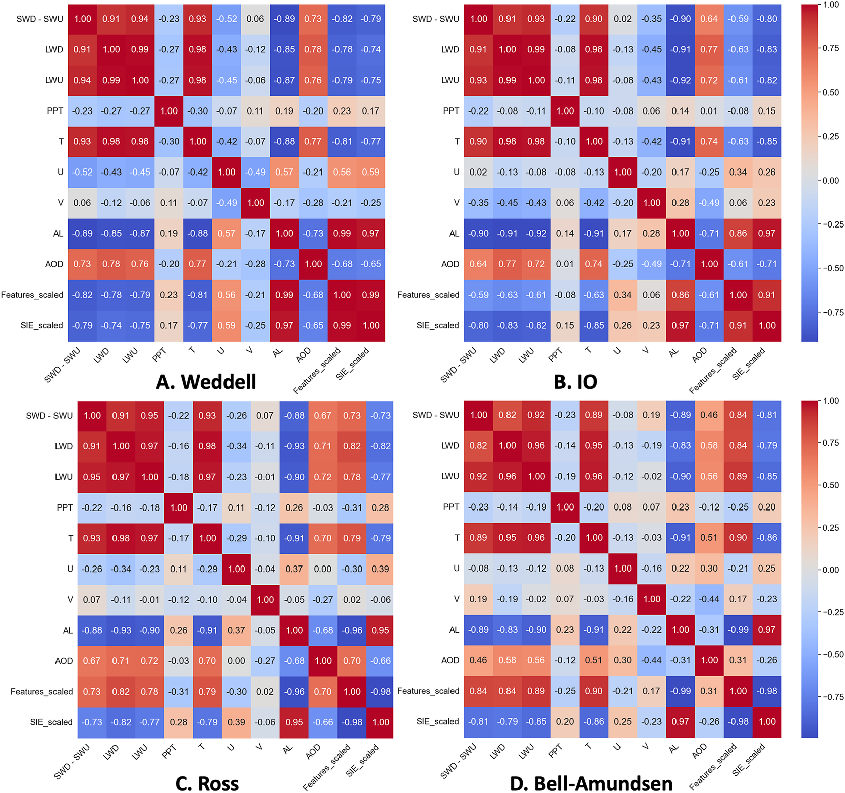
Figure 5. Heatmap showing the correlation among the features, SIE, Canonical loadings, and cross-loadings using canonical correlation analysis for the 2018 season. The correlations between the features and the canonical variate $ {Features}_{scaled} $ are called the canonical loadings. The correlations between the features and the canonical variate $ {SIE}_{scaled} $ are called the cross loadings. The color bar shows the strength of the positive (red) and negative (blue) correlations.

Table 3. Key features directly cause Sea Ice Extent in five different polar regions of the Antarctic basin

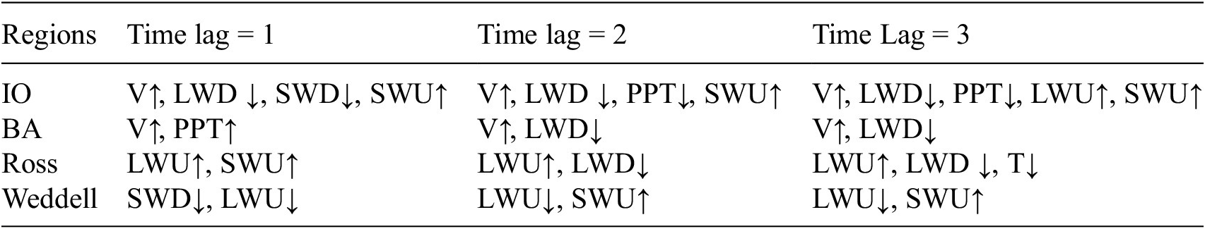
Note. The symbol $ \downarrow $ indicates negative inter-dependency and the symbol $ \uparrow $ indicates positive inter-dependency strength.

Figure 6. Heatmap showing the correlation among the features, SIE, Canonical loadings, and cross-loadings using canonical correlation analysis for the 2019 season. The correlations between the features and the canonical variate $ {Features}_{scaled} $ are called the canonical loadings. The correlations between the features and the canonical variate $ {SIE}_{scaled} $ are called cross-loadings. The color bar shows the strength of the positive (red) and negative (blue) correlations.

Figure 3a shows that over the Weddell region, SWD-SWU, LWU (longwave upward or emitted radiative flux), LWD (longwave downward radiative flux), Temperature (T), and relative humidity (Q) are the major factors impacting the SIE loss. In elastic net regression analysis, we use SWD and SWU separately to show the importance of SWU on SIE. The regression coefficients (Figure 4a) also match with the random forest analysis. SWU, LWU, LWD, T, and Q appear to have the largest coefficients. LWD is the LWU radiated back to the planet due to cloud cover and greenhouse gases. Owing to a strong dependency between LWU and T, the model penalizes the coefficient of T.

Similar feature importance is also observed over the IO region (Figure 3b). From random forest analysis, the most important features are SWD-SWU, LWD, and Q. Elastic net regression analysis also shows (Figure 4b) that the coefficients of SWU, LWD, and Q are the largest among all the parameters. Over the Ross region, the most important factors from random forest analysis (Figure 3c) appear to be SWD-SWU, LWD, and Q. From the elastic net regression analysis (Figure 4c), SWU, LWD, LWU, T, and Q are the most important factors that govern the melting. Over the BA region, SWD-SWU, LWD, LWU, and Q are the dominant features (Figures 3d and 4d). It appears that SWU or the reflected sunlight is a feature that consistently appears to be important from various methods. Although linear regression determines the coefficients of the features based on their correlation with the target variable (SIE) and the interdependency among the features, the signs of the features with larger coefficients bear some meaningful representation of their physical relationships. It is important to note that the coefficient of SWU is positive, which shows that SIE increases as more and more sunlight is reflected. Among other features that have higher coefficients, such as LWD, LWU, and T have negative coefficients since they have melting impacts on SIE.

The PCMCI + analysis aimed to unravel the intricate interactions governing these relationships, particularly concerning the sea ice extent as the parameter of interest. Table 3 summarizes the results from the causal discovery for three different lag times. In the Weddell Sea region, shortwave downward radiation (SWD) and longwave upward radiation (LWU) negatively influence sea ice extent ( $ \downarrow $ ) during lag = 1, while longwave upward radiation (LWU) negatively and shortwave upward radiation (SWU) positively impact sea ice extent ( $ \uparrow $ ) during lag =2 and 3. Thus, the causal discovery also confirms that the albedo effect (SWU) and temperature (or LWU and T) are two primary factors governing the SIE loss. As Table 3 shows, in the Indian Ocean region, the results indicate that increased wind speed (V) and SWU positively influence sea ice extent ( $ \uparrow $ ), while longwave downward radiation (LWD) negatively influences sea ice extent ( $ \downarrow $ ) at all-time lags. From causal discovery analysis, SWU, LWU, LWD, and T are directly causing SIE loss. Causal discovery analysis also shows that PPT (precipitation) and V (meridional wind) are directly related to SIE. However, their importance is not captured in the random forest and elastic net regression analyses. Over the Ross Sea region, longwave upward radiation (LWU) demonstrates a positive influence on sea ice extent ( $ \uparrow $ ) at all the time lags, while LWU has a negative influence over the Weddell region.

It appears that LWU has a positive impact only where LWD also appears to be important (Ross and IO). When LWD does not appear as an important feature, LWU has a negative impact on SIE due to LWU’s association with temperature. Both longwave downward radiation (LWD) and temperature (T) show negative effects ( $ \downarrow $ ) on SIE. It is interesting to note that over the BA region, SWU does not appear in the causal discovery despite a strong reduction in albedo and an increase in SWD-SWU (Figure 2). For the Bel/Amundsen Sea, wind speed (V) is found to have a positive influence on sea ice extent ( $ \uparrow $ ) at different time lags, where lag reflects the temporal variation of a feature’s effect on SIE. While longwave downward radiation (LWD) exhibits a negative impact ( $ \downarrow $ ) at time lags 2 and 3. Also, the results show precipitation (PPT) has a positive impact ( $ \uparrow $ ) at a time lag 1 on sea ice.

These findings shed light on the specific features and their causal influences on sea ice extent in the different polar regions of the Antarctic basin, highlighting the complex dynamics involved. The symbols $ \downarrow $ and $ \uparrow $ in Table 3 represent negative inter-dependency and positive inter-dependency strength, respectively, providing a clear representation of the causal relationships uncovered by the analysis. Although random forest and elastic net regression analyses are unable to capture that relationship, Table 3 indicates that SIE over the BA region depends on the large-scale features, cloud cover, and precipitation. Even though BA is located between the Ross and Weddell Seas, this did not appear to amplify the unusual behavior of sea ice extent. BC AARs and SIE loss over the BA region appear to be least connected possibly due to the heavy precipitation from atmospheric rivers in 2019 that contributed to a rapid increase in the snow height over the west Antarctic region Adusumilli et al. (2021). Rapid precipitation over the BA region appears to offset the impact of the BC aerosols.

It appears from random forest, elastic net regression, and causal discovery analyses that SWU has a strong effect on SIE over many of the regions over the Southern Ocean. Thus, the reduction in SIE in season19 is related to an increase in SWD-SWU over the ocean. An increase in SWD-SWU indicates an increase (decrease) in the absorption (reflection) of the incoming sunlight. This phenomenon should be connected with the albedo and aerosol optical depth (AOD) if the sea ice retreat in season19 is tied to the BC AARs. As a result, we now include two more features (albedo or Al and AOD) in our CCA analysis for season18 and season19 (Figures 5 and 6).

It is important to note that the findings on the feature importance from various methods used in this study (Random Forest Regression, Elastic Net Regression, and Causal Discovery) are in tandem with each other and also supported by multiple literature that used physics-based analysis to identify the importance of various features on sea ice retreat. Abrupt shifts in sea ice extent (SIE) are driven by record-breaking anomalous sea ice behavior, leading to a 28% reduction in SIE compared to the climatological mean in 2016—just one year after the retreat began Schroeter et al. (2023); Turner et al. (2017). But, studies are lacking to identify the reasons behind such abrupt loss in sea ice, especially the relative importance of various features that can affect SIE. Recent studies Eayrs et al. (2021); Purich et al. (2023) identify early spring advection of atmospheric heat and warm ocean waters as two key factors behind this rapid decline in SIE. Research has shown that anomalous atmospheric and sea ice circulation played a crucial role in the abrupt recessions of the Larsen A and B ice shelves Christie et al. (2022). Anomalous events can drastically accelerate the loss of both SIE and the Antarctic Ice Sheet compared to non-anomalous events. Studies have also reported that the changes in sea ice retreat is also due to strengthening poleward wind component, snow-darkening effects of aerosols Laluraj et al. (2020), weakening of the Southern Hemisphere mid-latitude westerlies, algal blooms Khan et al. (2021), El-Nino Southern Oscillation or ENSO, and the doubling of $ {CO}_2 $ Andrews and Forster (2020). Another recent study shows that the reflected solar radiation from Antarctic sea ice to space increased between 1991 and 2015, but started decreasing after 2016 due to surface albedo reduction in response to the reduced sea ice area. This highlights the importance of sea ice loss on radiative forcing Riihelä et al. (2021). However, no study has compared the relative influence of various atmospheric and oceanic features on sea ice retreat as shown in our study. This is a significant advancement that this study achieves by analyzing the satellite data sets using machine learning methods. To our knowledge, this has not been reported in previous studies.

Figure 5 shows the correlation heatmap of different features, SIE, and their canonical loadings as well as cross-loadings from CCA analysis. We have used nine different features, SWD-SWU or net solar energy, LWD, LWU, PPT, T, U, V, AL, and AOD. The correlations between the features and the canonical variate $ {Features}_{scaled} $ are called the canonical loadings. The correlations between the features and the canonical variate $ {SIE}_{scaled} $ are called the cross loadings (last column). From Figure 5, it appears that the radiative features (SWD-SWU, LWD, and LWU) are positively related to each other and temperature (T). Radiative features are negatively correlated with Albedo (AL) and the cross-loading ( $ {SIE}_{scaled} $ ). The correlation between AL and $ {SIE}_{scaled} $ (cross-loading) is the largest and almost close to 1 (0.97–0.98) over all the regions. These results suggest that as AL decreases, SWD-SWU increases, T increases, and SIE decreases. AOD is negatively correlated with AL. These results are expected and confirm the findings of Figure 2 that AOD due to the arrival of BC AARs decreases AL. Radiative features including T and net solar energy are also positively correlated with AOD, which indicates that AOD leads to a higher absorption of incoming solar energy or net solar energy (SWD-SWU). AOD is also strongly and negatively correlated with the cross-loading or $ {SIE}_{scaled} $ . As a result, as AOD increases due to the arrival of BC AARs, AL decreases, SWD-SWU increases, T increases, and SIE decreases. The strong negative correlation of features like AOD and net solar energy with the cross loading ( $ {SIE}_{scaled} $ ), positive correlations between AL the cross loading ( $ {SIE}_{scaled} $ ), and negative correlations between AOD and net solar energy with AL bolster our previous results and confirm the role of BC AARs on reductions in AL as well as reflected SWU and loss of SIE.

This is further confirmed in season19 (Figure 6) when it is observed that the correlations between AL and AOD also increase from −0.73, −0.71, −0.68, −0.31 in season18 to −0.86, −0.84, −0.87, −0.66 in season19 over the Weddell, IO, Ross, and BA regions, respectively. The correlations between SWD-SWU and AOD also increase in season19. AL continues to have a very strong ( $ \sim 1 $ ) correlation with $ {SIE}_{scaled} $ in season19. Moreover, the correlations between AOD and $ {SIE}_{scaled} $ increases from −0.65, −0.71, −0.66, and −0.26 in season18 to −0.84, −0.82, −0.85, and −0.67 in season19 over the Weddell, IO, Ross, and BA regions, respectively, as season19 experienced higher appearances of BC AARs. Our findings confirm the interconnections of BC AARs, AL, SWD-SWU, and SIE retreat over the Weddell, IO, and Ross regions. These correlations are the weakest over the BA region and are expected due to heavy precipitation leading to offsetting effects of snowfall on SIE as stated before. Moreover, a higher precipitation leads to the scavenging of aerosols. It appears that BA region is not affected by the presence of BC AARs in season19.

4.4. Anomalous melt events

In this study, we use various satellite SIE images and datasets to investigate the differences in anomalous melting events using the convolutional operation of CNN and discords using matrix profile, respectively. This is because, in addition to steady-state melting, anomalous melting events can contribute to a significantly higher melt in a short period of time. Figures 7a,b show that there was a higher number of discords noticed in season19, especially over the Weddell and Ross regions as expected from our results and also in tandem with the previous studies that cite that these two regions have been heavily impacted compared to any other regions Turner et al. (2020, 2022). The matrix profile was used for each grid cell using a time series of SIC data for a period of 23 years. Only the discords detected during season18 and season19 are shown here for interest. These findings are again confirmed by our convolutional operation of CNN analysis that shows a higher amount of anomalous melting events have been detected in season19 (Figures 7c,d). The matrix profile analysis is carried out on uniform 25 km resolution data, whereas the convolutional operation of CNN uses SIE images that have undergone through a discrete convolutional layer by $ 2\times 2 $ kernel and a pooling layer with pool size = (2, 2), stride = 2. We have selected the $ 2\times 2 $ kernel because each pixel represents a 25 km area, so the kernel covers a total of 100 km. Using a larger $ 3\times 3 $ kernel would cover 225 km, potentially losing precision. We have also evaluated other kernel sizes, such as $ 3\times 3 $ and $ 4\times 4 $ , but found that the $ 2\times 2 $ kernel provided the best results for our analysis. As a result, Figures 7c,d show a coarser resolution when we detect anomalous events as compared to Figures 7a,b that show discords at 25 km resolution. The reason behind the convolution and pooling operation is to identify neighborhoods with contiguous grids—all of which have experienced a similar high amount of SIE loss instead of a discrete grid as identified by the matrix profile. It appears from Figure 7 that some grids experience 5–20 anomalous and discord events, especially over the PC and BA regions. Other regions like the Weddell and Ross can experience as high as 30–50 anomalous events and discords. These results suggest that BC AARs might also have a significant impact on sea ice retreat. Both the metrics agree with each other in terms of the number of anomalous events and discords as well as the region where the effects are seen the most. It appears from the convolutional operation of CNN analysis that the anomalous melting events begin at the outer boundary of the sea ice extent in August and gradually engulf the entire region by the end of December, and by February, the number of anomalous events further intensifies (not shown). After February, the anomalous events decrease as austral winter approaches.

Figure 7. Anomalous melt events were detected by matrix profile for (a) season18 and (b) season19 and by convolutional operation of CNN for (c) season18 and (d) season19. The color bars show the number of such events.

5. Conclusion and discussion

This study detects the relationships between the role of the presence of BC AARs, darkening of the snow and ice or albedo reduction, and the relationship between the reflected sunlight to the SIE loss over Weddell, Ross, and IO region using various methods (random forest, elastic net regression, causal discovery, canonical correlation, matrix profile, and convolutional operation of CNN). Our results show that unusually higher numbers ( $ \sim 10 $ ) BC AARs arrived over the Antarctic region in season19 from the Amazon wildfire region as compared to season18. The Weddell region experienced the largest reduction in the sea ice extent during the presence of BC AARs. SIE losses over the Ross and IO regions were insignificantly different in season18 but were significantly higher during the presence of BC AARs in season19. The regions that experienced the presence of a higher number of BC AARs show a reduction in albedo and an increase in the net solar energy absorbed, except the Pacific Ocean Region. A higher number of BC AARs, high aerosol optical depth, reduced albedo, and enhanced absorbed sunlight are related to SIE loss over the Weddell, IO, and Ross regions along with LWU or the emitted longwave energy at the surface and temperature (T). AL is strongly correlated ( $ \sim 1 $ ) with SIE. AOD is negatively and strongly correlated with AL. A higher number of BC AARs are observed over the Ross, Weddell, and IO regions in season19, higher coefficients of SWU in the elastic net regression analysis, higher importance of SWU from the random forest analysis, and a positive and direct relationship between SWU and SIE in the causal discovery, and increased correlation coefficients between AOD with SWD-SWU, AL, and SIE in CCA analysis suggest that the sea ice albedo, as well as ice darkening by BC aerosols, are very important for sea ice extent over these regions.

Convolutional operation of CNN and matrix profile analyses were employed to visualize the anomalous melting events and discords over the region. Both the metrics using sea ice extent images and sea ice concentration data agree that a higher number of anomalous melting events have occurred during season19. Such findings also hint that there might be a connection between BC AARs and anomalous melting events or discords. Such an effect might be able to exacerbate the global warming effect and cause a larger number of anomalous melting in the future. This emphasizes the need to focus on this problem and take preventive actions to stop anthropogenic wildfires that may wreak havoc on sea ice extent and ice sheets in the future.

This is an unprecedented study that untangled an important fact about sea ice retreat using multiple satellite measurements. Our study points out that despite the fact that the Amazon is thousands of kilometers away from the Antarctic region, the slash-and-burn practices over the Amazon rainforest can severely impact the SIE that protects the land ice. We have employed six different methods, random forest regression, elastic net regression, causal discovery analysis, canonical correlation analysis, matrix profile analysis, and the convolutional operation of CNN. All the methods confirm the same findings. This effect can amplify the global warming effect on sea ice that is already causing extensive sea ice as well as ice sheet disappearances. The relative influence of BC aerosols, global warming, and associated changes in other features on SIE needs to be explored to untangle their role in sea level rise. In the future, such practices will severely impact the already shrinking ice concentration, amplify the ice sheet melting both over the land and sea, and amplify the sea level rise.

Further analysis is needed to understand how precipitation offsets the BC AAR effect over the BA region despite a strong presence of enhanced numbers of BC AARs. BA regions show the weakest relationships between AOD, AL, SWD-SWU, and SIE loss. LWD represents a fraction of LWU radiated back to Earth by clouds. LWU has a positive impact on SIE only when the coefficient of LWD is high, presumably because LWU acts as a measure of getting rid of the heat in cloudy conditions. Further analysis is required to tease out the impacts from LWD and LWU under clear-sky and cloudy conditions. However, this is beyond the scope of this study. Our study detects anomalous melting events using the convolutional operation of the CNN method, which is an adaptation from our article Devnath et al. (2024). In the future, we will employ our convolutional operation of the CNN method to detect the steady state melting (melting rate close to the mean melting) over these regions and will extend the concept of the inverse max pooling method by applying multiple hidden layers in a full CNN model to predict anomalous melting events and detect neighborhood that are prone to anomalous melting events during and presence of BC AARs. These will be addressed in future studies with a focus on the similar effects on ice sheets that cause the sea level to rise. Furthermore, it appears from the causal discovery that some features become important as the lag time varies. It needs further analysis to identify how different features become important after the BC AAR occurrences.

Sudip Chakraborty designed the research, analyzed the data, and wrote the article. Maloy Kumar Devnath analyzed the data, Atefeh Jabeli analyzed the data, Chhaya Kulkarni analyzed the data, Gehan Boteju analyzed the data, Jianwu Wang contributed to writing the article and designing the research, Vandana P. Janeja contributed to writing the article and designing the research.