


1 Introduction
Imagine you are faced with a challenging decision and you have the option of assembling a large group of people whose goal is to identify the best possible choice with a high degree of accuracy. Would you prefer to assemble a group of more competent individuals or one that is more diverse? According to the well-known Diversity-Trumps-Ability Theorem (DTA), when comparing two groups of similar size, the more diverse group will generally outperform the more competent group.
Since its publication nearly two decades ago (Hong and Page Reference Hong and Page2004), the DTA has received considerable attention, though it has also faced substantial criticism regarding its mathematical rigor (Thompson Reference Thompson2014). Nevertheless, the theorem has sparked widespread discussion in a number of disciplines, including the social sciences, humanities, and computer science.
Most notably, Hélène Landemore (Reference Landemore2012) employs the DTA in defense of democracy. Interpreting the theorem to suggest that a diverse group of less competent individuals can generally outperform a group of highly skilled experts, she argues that democratic processes are likely to produce superior decisions compared to those made by a small group of experts (Christiano and Bajaj Reference Christiano, Bajaj, Zalta and Nodelman2024). In doing so, Landemore aligns the DTA with similar arguments within the realm of epistemic democracy, which studies and defends democracy based on its ability to effectively track the truth (Sakai Reference Sakai2020). This is akin to the Condorcet Jury Theorem (CJT) (Genta Reference Genta2024), which, under fairly restrictive assumptions, posits that as the number of voters increases, the probability of the group identifying the correct option converges toward 1.
Discussions of DTA and diversity in decision-making typically focus on three different epistemic frameworks: search problems, deliberation, and voting (Niesen et al. Reference Niesen, Spiekermann, Herzog, Girard and Vogelmann2024). In this paper, we focus specifically on voting, understood as an election mechanism involving a set of voters, a set of options, and the aggregation of the voters’ selected choices (Niesen et al. Reference Niesen, Spiekermann, Herzog, Girard and Vogelmann2024).
While most works discussing the DTA tend to either (i) explore its implications within their respective fields, (ii) highlight its formal limitations, or (iii) perform experimental simulations to validate or challenge its claims, our contribution focuses on offering mathematically rigorous bounds that specify the conditions under which diversity truly exceeds ability.
More specifically, we first embed the DTA problem in a voting model that operates within the framework of the CJT. This serves three purposes: (1) it forms a bridge between two of the main arguments in the field of epistemic democracy, (2) it allows to clearly define diversity in a voting setting, associating the increasing influence of a so-called opinion leader on the electorate with a decrease in diversity, (3) it provides probabilistic guarantees for the identification of the correct option, which depend on this notion of diversity.
Second, within this model we derive a precise threshold for when diversity truly exceeds ability, inspired by techniques recently introduced by Karge (Reference Karge, Arisaka, Sanchez-Anguix, Stein, Aydoğan, van der Torre and Ito2024), where similar bounds are derived for a scenario involving the aggregation of imprecise probabilistic beliefs.
Finally, we devote a section to positioning our results within the philosophical framework of epistemic democracy. In this section, we (1) revisit the long-standing relationship between epistemic democracy and the CJT, (2) provide an overview of key generalizations of the CJT, and (3) examine its connection to the DTA. In each case, we highlight how our results contribute to the ongoing discussion.
2 Preliminaries
In this section, we introduce the notation and formal foundations of this paper. To ensure accessibility, we present the preliminaries to our framework in natural language wherever possible, focusing only on the parameters essential to the main discussion. For a formal treatment of the underlying framework, we refer the reader to section 7.1 in the appendix.
We begin by introducing the CJT, a central result from the epistemic view of voting. This is done in three parts: First, we present the original CJT result, and second, we discuss a recently proposed generalization that simultaneously weakens all of the original assumptions. Finally, we define diversity and ability within this framework.
The CJT. As a fundamental theorem in voting theory, the CJT provides probabilistic guarantees for determining the presumed correct alternative among a set of alternatives under certain conditions. Originally, the CJT assumed that agents are equally competent (homogeneity), that they are more likely to vote for the correct alternative than for a competitor (reliability), that they do not influence each other or be influenced by an external factor in the voting process (independence), and that they choose exactly one (completeness) out of two alternatives (dichotomy) in majority voting. Thus the classic CJT (Condorcet Reference Condorcet1785) states the following.
Theorem 1 (Condorcet Reference Condorcet1785). For odd-numbered, homogeneous groups of independent and reliable agents in a dichotomic voting setting, the probability that majority voting identifies the correct alternative
-
(1) increases monotonically with the number of agents and
-
(2) converges to $1$
as the number of agents goes to infinity.
$1$
as the number of agents goes to infinity.

Since the real world cannot guarantee these ideal conditions, it is essential in CJT research to seek generalizations that maintain the asymptotic part under weakened assumptions, while the monotonic increase fails once heterogeneously competent agents are allowed (Owen et al. Reference Owen, Grofman and Feld1989).
Recently, a novel generalization of CJT has been proposed that simultaneously weakens all of the assumptions underlying the original CJT (Karge et al. Reference Karge, Arisaka, Sanchez-Anguix, Stein, Aydoğan, van der Torre and Ito2024). In this generalization, agents are allowed to vote for an arbitrary finite number of alternatives, while allowing for heterogeneous competence levels and a degree of correlation among voters modeled by an opinion leader (OL), the classic dependency model in the CJT literature (Boland et al. Reference Boland, Proschan and Tong1989).
The opinion leader (OL) serves as an abstract external influence in the voting process, without actively participating in it. Instead, the OL approves or disapproves presented alternatives based on her own competence $\hat p$
, which represents the probability of approving the correct alternative. Subsequently, her choice influences the votes of the agents: each agent votes according to the preference of the OL rather than her own “inner voice” with a certain probability
$\hat p$
, which represents the probability of approving the correct alternative. Subsequently, her choice influences the votes of the agents: each agent votes according to the preference of the OL rather than her own “inner voice” with a certain probability $\pi $
. In the standard OL model, this probability
$\pi $
. In the standard OL model, this probability $\pi $
is identical for all agents, i.e., it is uniformly distributed.
$\pi $
is identical for all agents, i.e., it is uniformly distributed.
2.1 Voting probabilistic framework
We now introduce the underlying voting and probabilistic framework.
Let $\;{\cal W} = \left\{ {{\omega _1}, \ldots, {\omega _m}} \right\}$
denote a finite set of
$\;{\cal W} = \left\{ {{\omega _1}, \ldots, {\omega _m}} \right\}$
denote a finite set of $m$
alternatives. For example, in a political context, each
$m$
alternatives. For example, in a political context, each ${\omega _j}$
could represent a policy that can be voted on. Moreover, we define a finite set
${\omega _j}$
could represent a policy that can be voted on. Moreover, we define a finite set ${\cal N} = \left\{ {{a_1}, \ldots, {a_n}} \right\}$
consisting of
${\cal N} = \left\{ {{a_1}, \ldots, {a_n}} \right\}$
consisting of $n$
agents. The underlying voting method in our model is approval voting, where each agent
$n$
agents. The underlying voting method in our model is approval voting, where each agent ${a_i}$
can vote for any number of alternatives from the set
${a_i}$
can vote for any number of alternatives from the set ${\cal W}$
. In a given election, the alternative that receives the most votes wins the approval vote.
${\cal W}$
. In a given election, the alternative that receives the most votes wins the approval vote.
Example 1. Suppose we have $m = 3$
alternatives, i.e.,
$m = 3$
alternatives, i.e., $\;{\cal W} = \left\{ {{\omega _1},{\omega _2},{\omega _3}} \right\}$
and that we have
$\;{\cal W} = \left\{ {{\omega _1},{\omega _2},{\omega _3}} \right\}$
and that we have $n = 2$
agents, i.e.,
$n = 2$
agents, i.e., ${\cal N} = \left\{ {{a_1},{a_2}} \right\}$
. Suppose
${\cal N} = \left\{ {{a_1},{a_2}} \right\}$
. Suppose ${a_1}$
votes for the alternatives
${a_1}$
votes for the alternatives ${\omega _1},{\omega _2},$
and
${\omega _1},{\omega _2},$
and ${a_2}$
votes only for
${a_2}$
votes only for ${\omega _1}$
. Then
${\omega _1}$
. Then ${\omega _1}$
has a strictly higher score than either of the competing alternatives and wins the approval vote.
${\omega _1}$
has a strictly higher score than either of the competing alternatives and wins the approval vote.
Within the set ${\cal W}$
, we assume that exactly one alternative is correct, denoted as
${\cal W}$
, we assume that exactly one alternative is correct, denoted as ${\omega _{\rm{*}}}$
. Given this fixed alternative, the voting scenario unfolds as a random process that determines both the opinion leader’s (OL) approved choices and the agents’ votes. First, the OL endorses a subset of alternatives without directly participating in the voting process. The probability that the OL includes the correct alternative in this subset is given by
${\omega _{\rm{*}}}$
. Given this fixed alternative, the voting scenario unfolds as a random process that determines both the opinion leader’s (OL) approved choices and the agents’ votes. First, the OL endorses a subset of alternatives without directly participating in the voting process. The probability that the OL includes the correct alternative in this subset is given by $\hat p$
, representing her competency. Second, each agent independently selects a subset of alternatives before casting their vote, with the probability of correctly identifying
$\hat p$
, representing her competency. Second, each agent independently selects a subset of alternatives before casting their vote, with the probability of correctly identifying ${\omega _{\rm{*}}}$
determined by the parameter
${\omega _{\rm{*}}}$
determined by the parameter $p_i^{{\omega _{\rm{*}}}}$
. Finally, a fraction of the agents follows the OL’s endorsements, meaning their final votes align with the alternatives approved by the OL. The likelihood of an agent adhering to the OL’s choices is captured by the parameter
$p_i^{{\omega _{\rm{*}}}}$
. Finally, a fraction of the agents follows the OL’s endorsements, meaning their final votes align with the alternatives approved by the OL. The likelihood of an agent adhering to the OL’s choices is captured by the parameter $\pi $
, which is assumed to be uniform across all agents. Once the subset of OL-following agents is established, the final voting occurs: each agent either votes according to their private selection or adopts the OL’s approved alternatives.
$\pi $
, which is assumed to be uniform across all agents. Once the subset of OL-following agents is established, the final voting occurs: each agent either votes according to their private selection or adopts the OL’s approved alternatives.
Example 2. We provide some example values for each parameter: Suppose that the OL has a rather high probability of approving the correct alternative $\hat p = 0.6$
and that agents are relatively inclined to follow the OL
$\hat p = 0.6$
and that agents are relatively inclined to follow the OL $\pi = 0.4$
. Suppose also that
$\pi = 0.4$
. Suppose also that ${a_1}$
has a high probability of voting for the first two alternatives when uninfluenced, but never votes for the third:
${a_1}$
has a high probability of voting for the first two alternatives when uninfluenced, but never votes for the third: $p_1^{{\omega _1}} = 0.8,p_1^{{\omega _1}} = 0.75,p_1^{{\omega _1}} = 0$
.
$p_1^{{\omega _1}} = 0.8,p_1^{{\omega _1}} = 0.75,p_1^{{\omega _1}} = 0$
.
To derive the generalized CJT result, two additional assumptions are required. The first, known as $\Delta p$
-group reliability, is defined in terms of the average probability that an agent privately approves the correct alternative, denoted as
$\Delta p$
-group reliability, is defined in terms of the average probability that an agent privately approves the correct alternative, denoted as ${{\bar p}^{{\omega _{\rm{*}}}}}$
, and the corresponding probability for any incorrect alternative, denoted as
${{\bar p}^{{\omega _{\rm{*}}}}}$
, and the corresponding probability for any incorrect alternative, denoted as ${{\bar p}^{{\omega _\dagger}}}$
. The
${{\bar p}^{{\omega _\dagger}}}$
. The ${\rm{\Delta }}p$
-group reliability assumption states that
${\rm{\Delta }}p$
-group reliability assumption states that ${{\bar p}^{{\omega _{\rm{*}}}}}$
must exceed
${{\bar p}^{{\omega _{\rm{*}}}}}$
must exceed ${{\bar p}^{{\omega _\dagger}}}$
by at least a margin of
${{\bar p}^{{\omega _\dagger}}}$
by at least a margin of ${\rm{\Delta }}p$
for any incorrect alternative.
${\rm{\Delta }}p$
for any incorrect alternative.
The second assumption, referred to as private agent approval independence, requires that each agent’s private selection of an alternative occurs independently, ensuring that agents do not influence one another in this process. However, this does not imply independence in the final election outcome; agents’ choices may still be correlated through the influence of the opinion leader.
Based on these assumptions, a bound on the worst-case minimum probability of success, ${P_{{\rm{min}}}}$
, for identifying the correct alternative through approval voting can be established (Karge et al. Reference Karge, Arisaka, Sanchez-Anguix, Stein, Aydoğan, van der Torre and Ito2024). Throughout this paper, we interpret an increase in
${P_{{\rm{min}}}}$
, for identifying the correct alternative through approval voting can be established (Karge et al. Reference Karge, Arisaka, Sanchez-Anguix, Stein, Aydoğan, van der Torre and Ito2024). Throughout this paper, we interpret an increase in ${\rm{\Delta }}p$
as a rise in average competence, while a higher
${\rm{\Delta }}p$
as a rise in average competence, while a higher $\pi $
reflects greater correlation among agents.
$\pi $
reflects greater correlation among agents.
Theorem 2 Consider an approval voting setting with $m \gt 1$
alternatives, satisfying private agent approval independence and
$m \gt 1$
alternatives, satisfying private agent approval independence and $\Delta p$
-group reliability for some
$\Delta p$
-group reliability for some $\Delta p \in \left( {0,1} \right]$
, influenced by an opinion leader with
$\Delta p \in \left( {0,1} \right]$
, influenced by an opinion leader with $\pi \in \left[ {0,{{\Delta p} \over {\Delta p + 1}}} \right)$
and
$\pi \in \left[ {0,{{\Delta p} \over {\Delta p + 1}}} \right)$
and $\hat p \in \left[ {0,1} \right]$
. Then it is guaranteed that the success probability of the approval voting process is at least
$\hat p \in \left[ {0,1} \right]$
. Then it is guaranteed that the success probability of the approval voting process is at least
 $$1 - \left( {m - 1} \right)\left( {\hat p{e^{ - {1 \over 2}n{\rm{\Delta }}{p^2}{{(1 - \pi )}^2}}} + \left( {1 - \hat p} \right){e^{ - {1 \over 2}n{{({\rm{\Delta }}p\left( {1 - \pi } \right) - \pi )}^2}}}} \right).$$
Observe that, in order to guarantee that the minimal success probability converges to one as the number of agents goes to infinity, a bound on the probability of following the OL is required, i.e., $\pi \in \left[ {0,{{\Delta p} \over {\Delta p + 1}}} \right)$
. This theorem will play a crucial role in determining the threshold for when DTA later in the paper. To see how a combination of different parameters yields a minimum probability of success, called
$\pi \in \left[ {0,{{\Delta p} \over {\Delta p + 1}}} \right)$
. This theorem will play a crucial role in determining the threshold for when DTA later in the paper. To see how a combination of different parameters yields a minimum probability of success, called ${P_{min}}$
, consider the following example:
${P_{min}}$
, consider the following example:
Example 3. Consider the following parameters: Suppose we have a relatively large number of alternatives, $m = 20$
, and a set of agents who, on average, are 40% more likely to vote for the correct alternative than for any other,
$m = 20$
, and a set of agents who, on average, are 40% more likely to vote for the correct alternative than for any other, ${\rm{\Delta }}p = 0.4$
. Suppose also that we have a very competent OL who approves the correct alternative with a probability of 80%, i.e.,
${\rm{\Delta }}p = 0.4$
. Suppose also that we have a very competent OL who approves the correct alternative with a probability of 80%, i.e., $\hat p = 0.8$
. Finally, suppose we have 100 agents, where each agent has a 10% chance of following the OL:
$\hat p = 0.8$
. Finally, suppose we have 100 agents, where each agent has a 10% chance of following the OL: $\pi = 0.1$
, and
$\pi = 0.1$
, and $n = 100$
. This gives a minimum probability of success for the correct alternative to win the approval vote of
$n = 100$
. This gives a minimum probability of success for the correct alternative to win the approval vote of ${P_{{\rm{min}}}} = 0.85$
.
${P_{{\rm{min}}}} = 0.85$
.
Naturally, the minimum probability of success can be adjusted by modifying these parameters. Intuitively, ${P_{{\rm{min}}}}$
increases with a larger number of agents, as this amplifies the wisdom of the crowds effect, and with higher competency levels among both the agents and the opinion leader. Additionally, reducing the number of alternatives improves the likelihood of identifying the correct one, as fewer options generally make the correct choice easier to discern. Finally, the success probability increases when the likelihood of agents following the opinion leader decreases. This is because our bound represents a worst-case scenario where, in the worst case, the opinion leader selects only incorrect alternatives, causing the electorate to be misled toward these wrong choices.
${P_{{\rm{min}}}}$
increases with a larger number of agents, as this amplifies the wisdom of the crowds effect, and with higher competency levels among both the agents and the opinion leader. Additionally, reducing the number of alternatives improves the likelihood of identifying the correct one, as fewer options generally make the correct choice easier to discern. Finally, the success probability increases when the likelihood of agents following the opinion leader decreases. This is because our bound represents a worst-case scenario where, in the worst case, the opinion leader selects only incorrect alternatives, causing the electorate to be misled toward these wrong choices.
Having defined the underlying formal framework, we now define the two concepts central to this work, diversity and ability.
When it comes to diversity, there are a variety of ways to find an appropriate model. Within voting, a common approach is to model diversity as a lack of positive correlation that affects all voters in the same way, as in the OL model (Niesen et al. Reference Niesen, Spiekermann, Herzog, Girard and Vogelmann2024). Ability, on the other hand, is more straightforward. In a truth-tracking voting setting, we let ability refer to the probability of an agent identifying the correct alternative, i.e., with the agent’s uninfluenced competence.
Definition 1 (Diverse Groups). Consider two groups of equal size, i.e., both groups compromise the same number of agents. Let ${\pi _1}$
and
${\pi _1}$
and ${\pi _2}$
denote the uniformly distributed probabilities of following the OL for group 1 and group 2, respectively. We say that group 1 is more diverse than group 2 if
${\pi _2}$
denote the uniformly distributed probabilities of following the OL for group 1 and group 2, respectively. We say that group 1 is more diverse than group 2 if ${\pi _1} \lt {\pi _2}$
, i.e., if the first group has a lower positive correlation than the second.
${\pi _1} \lt {\pi _2}$
, i.e., if the first group has a lower positive correlation than the second.
In the subsequent step, a group of agents with higher levels of competence or expertise is defined.
Definition 2 (Competent Groups). Given two groups of equal size. Let $\Delta {p_1}$
and
$\Delta {p_1}$
and $\Delta {p_2}$
denote the margins by which each group is, on average, more likely to vote for the correct alternative than a competitor. We say that group 1 is more competent than group 2 if
$\Delta {p_2}$
denote the margins by which each group is, on average, more likely to vote for the correct alternative than a competitor. We say that group 1 is more competent than group 2 if $\Delta {p_1} \gt \Delta {p_2}$
.
$\Delta {p_1} \gt \Delta {p_2}$
.
With these definitions in hand, we proceed to derive a threshold for when diversity exceeds ability or competence.
3 A diversity threshold
In this section, our goal is to delineate an exact threshold for when diversity truly exceeds ability within the Condorcet voting model.
Recall the original problem statement: You want to assemble a group of experts that is either more diverse or more competent. Suppose your group already consists of a few agents, and you want to increase the diversity, i.e., reduce the uniformly distributed probability, $\pi $
, of following the OL. Since it may not seem reasonable on a conceptual level to claim that adding another agent will reduce this uniform value across the group, we resort to a recent extension (Karge Reference Karge, Arisaka, Sanchez-Anguix, Stein, Aydoğan, van der Torre and Ito2024) of the CJT model of Theorem 2. This extension generalizes the bound on the minimum probability of success for a uniform
$\pi $
, of following the OL. Since it may not seem reasonable on a conceptual level to claim that adding another agent will reduce this uniform value across the group, we resort to a recent extension (Karge Reference Karge, Arisaka, Sanchez-Anguix, Stein, Aydoğan, van der Torre and Ito2024) of the CJT model of Theorem 2. This extension generalizes the bound on the minimum probability of success for a uniform $\pi $
-value to allow for an average probability of following the OL and also allows for a meaningful discussion of the potential increase or decrease in correlation within a group of agents. In the following, we first introduce this generalization, following the exposition of Karge (Reference Karge, Arisaka, Sanchez-Anguix, Stein, Aydoğan, van der Torre and Ito2024), and then use this bound to derive the desired threshold.
$\pi $
-value to allow for an average probability of following the OL and also allows for a meaningful discussion of the potential increase or decrease in correlation within a group of agents. In the following, we first introduce this generalization, following the exposition of Karge (Reference Karge, Arisaka, Sanchez-Anguix, Stein, Aydoğan, van der Torre and Ito2024), and then use this bound to derive the desired threshold.
3.1 Extending the CJT to average opinion leader influence
As a first step towards this generalization, the original OL framework is extended to allow for a finite number of different $\pi $
-values (
$\pi $
-values ( ${\pi _1}, \ldots, {\pi _k}, \ldots {\pi _s}$
), where
${\pi _1}, \ldots, {\pi _k}, \ldots {\pi _s}$
), where $1 \le s \le n$
. This means that at most each agent can have its own
$1 \le s \le n$
. This means that at most each agent can have its own $\pi $
value. In a next step, the whole electorate is divided into different subgroups, where each subgroup compromises exactly those agents that have the same
$\pi $
value. In a next step, the whole electorate is divided into different subgroups, where each subgroup compromises exactly those agents that have the same $\pi $
-value.
$\pi $
-value.
Each subgroup is denoted by ${{\cal G}_{{\pi _k}}}$
, where
${{\cal G}_{{\pi _k}}}$
, where ${\pi _k}$
represents the exact
${\pi _k}$
represents the exact $\pi $
-value of that subgroup, such that
$\pi $
-value of that subgroup, such that
 $${{\cal G}_{{\pi _1}}} \cup \ldots {{\cal G}_{{\pi _k}}} \ldots \cup {{\cal G}_{{\pi _s}}} = {\cal N} = \left\{ {{a_1}, \ldots, {a_n}} \right\}.$$
This is illustrated in the following example.
Example 4. Let’s consider ten agents ( ${a_1}, \ldots, {a_{10}}$
) and four different
${a_1}, \ldots, {a_{10}}$
) and four different $\pi - $
values (
$\pi - $
values ( ${\pi _1} = 0.05,{\pi _2} = 0.1,{\pi _3} = 0.15,{\pi _4} = 0.9$
). One possible distribution of agents to subgroups could be:
${\pi _1} = 0.05,{\pi _2} = 0.1,{\pi _3} = 0.15,{\pi _4} = 0.9$
). One possible distribution of agents to subgroups could be: ${{\cal G}_{{\pi _1}}} = \left\{ {{a_1},{a_2},{a_3}} \right\},{{\cal G}_{{\pi _2}}} = \left\{ {{a_4},{a_5}} \right\},{{\cal G}_{{\pi _3}}} = \left\{ {{a_6},{a_7},{a_8},{a_9}} \right\},{{\cal G}_{{\pi _4}}}$ $ = \left\{ {{a_{10}}} \right\}$
.
$ = \left\{ {{a_{10}}} \right\}$
.
In this case, agents 1-3 follow the OL with probability 0.05, agents 4 and 5 with probability 0.1, and so on.
For each subgroup ${{\cal G}_{{\pi _k}}}$
, the number of agents in that subgroup is referred to as
${{\cal G}_{{\pi _k}}}$
, the number of agents in that subgroup is referred to as $\left| {{{\cal G}_{{\pi _k}}}} \right|$
. From this, it is straightforward to define the average
$\left| {{{\cal G}_{{\pi _k}}}} \right|$
. From this, it is straightforward to define the average $\pi $
-value,
$\pi $
-value, ${\bar \pi }$
as follows.
${\bar \pi }$
as follows.
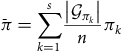 $$\bar \pi = \mathop \sum \limits_{k = 1}^s {{\left| {{{\cal G}_{{\pi _k}}}} \right|} \over n}{\pi _k}$$
That is, the average probability of following the opinion leader across all subgroups is the sum of all $\pi $
values, one for each subgroup, weighted by the number of agents in that subgroup.
$\pi $
values, one for each subgroup, weighted by the number of agents in that subgroup.
Finally, this leads to a bound on the minimal success probability that accounts for average OL influence (Karge Reference Karge, Arisaka, Sanchez-Anguix, Stein, Aydoğan, van der Torre and Ito2024).
Theorem 3 Consider an approval voting setting as described in Theorem 2, but allowing for different ${\pi _k}$
-values as defined above. Then it is guaranteed that the success probability of the approval voting process is at least
${\pi _k}$
-values as defined above. Then it is guaranteed that the success probability of the approval voting process is at least
 $$1 - \left( {m - 1} \right)\left( {\hat p\left( {{e^{ - {2 \over {4n}}{{\left( {\Delta p\left( {\sum\nolimits_{k = 1}^s {\left| {{G_{{\pi _k}}}} \right|} \left( {1 - {\pi _k}} \right)} \right)} \right)}^2}}}} \right) + \left( {1 - \hat p} \right){e^{ - {2 \over {4n}}\left( {\sum\nolimits_{k = 1}^s {\left| {{G_{{\pi _k}}}} \right|} (\Delta p\left( {1 - {\pi _k}} \right) - {\pi _k}){)^2}} \right).}}} \right.$$
Similar to Karge (Reference Karge, Arisaka, Sanchez-Anguix, Stein, Aydoğan, van der Torre and Ito2024), this bound can be shown to be equivalent in the worst case to the bound in Theorem 2. That is, if the uniformly distributed $\pi $
-value is equal to the average
$\pi $
-value is equal to the average $\bar \pi $
, then the minimum probability of success is the same, denoted by
$\bar \pi $
, then the minimum probability of success is the same, denoted by ${P_{min,\pi }} = {P_{min,\bar \pi }}$
. This result then allows to use the bound of Theorem 2 for actual calculations, as it is somewhat easier to work with, but also allows to discuss an increase or decrease of the correlation on a conceptual level when using Theorem 2.
${P_{min,\pi }} = {P_{min,\bar \pi }}$
. This result then allows to use the bound of Theorem 2 for actual calculations, as it is somewhat easier to work with, but also allows to discuss an increase or decrease of the correlation on a conceptual level when using Theorem 2.
Theorem 4 If $\pi = \bar \pi $
, then
$\pi = \bar \pi $
, then ${P_{min,\pi }} = {P_{min,\bar \pi }}$
.
${P_{min,\pi }} = {P_{min,\bar \pi }}$
.
Proof The proof can be found in the appendix, section 1. The implications of this theorem are illustrated in the following example.
Example 5. Consider again the group of ten agents and four subgroups from the previous example. The average probability of following the OL is $\bar \pi = 0.185$
. Suppose we have a very competent OL and a highly competent group of agents voting on three alternatives:
$\bar \pi = 0.185$
. Suppose we have a very competent OL and a highly competent group of agents voting on three alternatives: $\hat p = 0.9,{\rm{\Delta }}p = 0.7,m = 3$
. Due to Theorem 4, we may now invoke Theorem 2 to compute
$\hat p = 0.9,{\rm{\Delta }}p = 0.7,m = 3$
. Due to Theorem 4, we may now invoke Theorem 2 to compute ${P_{min}}$
, the minimal success probability. This yields that worst-case minimum probability of identifying the correct alternative according to Theorem 2 is then 0.55.
${P_{min}}$
, the minimal success probability. This yields that worst-case minimum probability of identifying the correct alternative according to Theorem 2 is then 0.55.
3.2 A diversity threshold
Next, we want to determine the threshold at which increased diversity increases the group’s capabilities relative to a more competent group. The derivation for this threshold can be found in the Appendix in section 7.3. Intuitively, to determine this threshold we introduce the parameter $\varepsilon $
, which represents the amount by which the average correlation is smaller in the more diverse group. Similarly,
$\varepsilon $
, which represents the amount by which the average correlation is smaller in the more diverse group. Similarly, $\lambda $
represents the increase in competency in the less diverse group. The more diverse group outperforms the more competent one as soon as the minimal success probability,
$\lambda $
represents the increase in competency in the less diverse group. The more diverse group outperforms the more competent one as soon as the minimal success probability, ${P_{min}}$
is greater. This is the case when the increase in
${P_{min}}$
is greater. This is the case when the increase in ${P_{min}}$
due to the increase in diversity exceeds the increase in
${P_{min}}$
due to the increase in diversity exceeds the increase in ${P_{min}}$
due to the increase in the competence of the agents. This is the case when:
${P_{min}}$
due to the increase in the competence of the agents. This is the case when:
 $$\varepsilon \ge {{\lambda - \pi \lambda } \over {\Delta p + 1}}$$
This directly yields the following corollary which specifies when exactly DTA in our model.
Corollary 1 In an approval voting setting as described in Theorem 2, and provided diversity and ability are defined as in Definitions 1 and 2, DTA if inequality 1 is true.
We illustrate this threshold for an example setting in Figure 1, where we have 100 fairly competent agents voting on five alternatives with a moderately influential OL, where the first group is slightly more competent and where we vary the increase in diversity for the second group, i.e., $n = 100,m = 5,{\rm{\Delta }}p = 0.5,\pi = 0.2,\lambda = 0.1$
.
$n = 100,m = 5,{\rm{\Delta }}p = 0.5,\pi = 0.2,\lambda = 0.1$
.
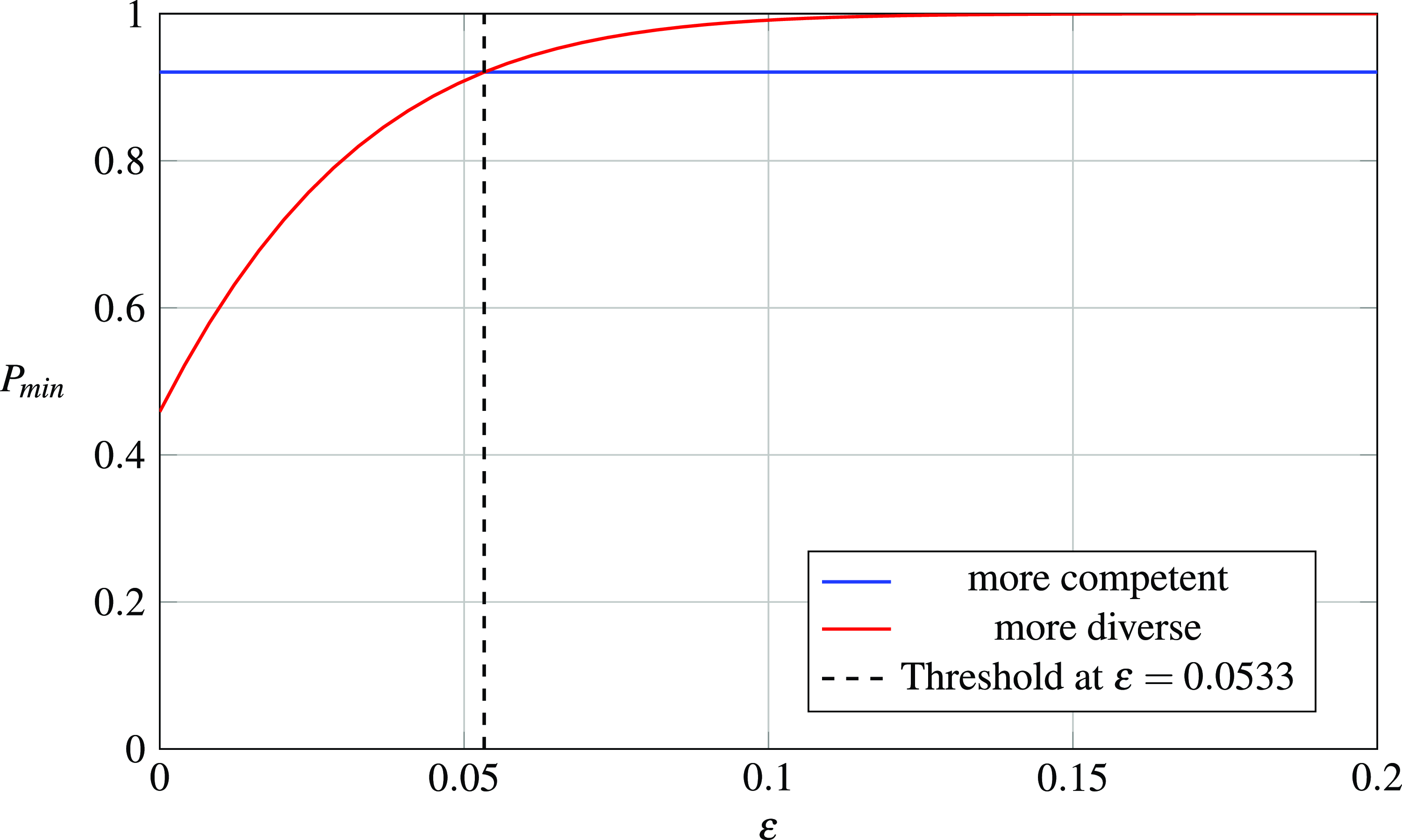
Figure 1. Plot of success probability of a more competent group (blue) and a more diverse group (red) for varying $\varepsilon $
.
$\varepsilon $
.
From the plot, we can see that in this particular setting, even a small increase in diversity (decrease in $\pi $
) causes the more diverse group to outperform the more competent group.
$\pi $
) causes the more diverse group to outperform the more competent group.
We further illustrate in Figure 2 for the same scenario, i.e., $n = 100,m = 5,{\rm{\Delta }}p = 0.5,\pi = 0.2$
, a simultaneous increase in competence and diversity. In this plot, a value greater than 0 indicates that the more competent group outperforms the more diverse group (e.g., at
$n = 100,m = 5,{\rm{\Delta }}p = 0.5,\pi = 0.2$
, a simultaneous increase in competence and diversity. In this plot, a value greater than 0 indicates that the more competent group outperforms the more diverse group (e.g., at $\lambda = 0.2,\varepsilon = 0$
), and conversely, a value less than 0 indicates that the more diverse group outperforms the more competent group (e.g., at
$\lambda = 0.2,\varepsilon = 0$
), and conversely, a value less than 0 indicates that the more diverse group outperforms the more competent group (e.g., at $\lambda = 0.1,\varepsilon = 0.2$
).
$\lambda = 0.1,\varepsilon = 0.2$
).
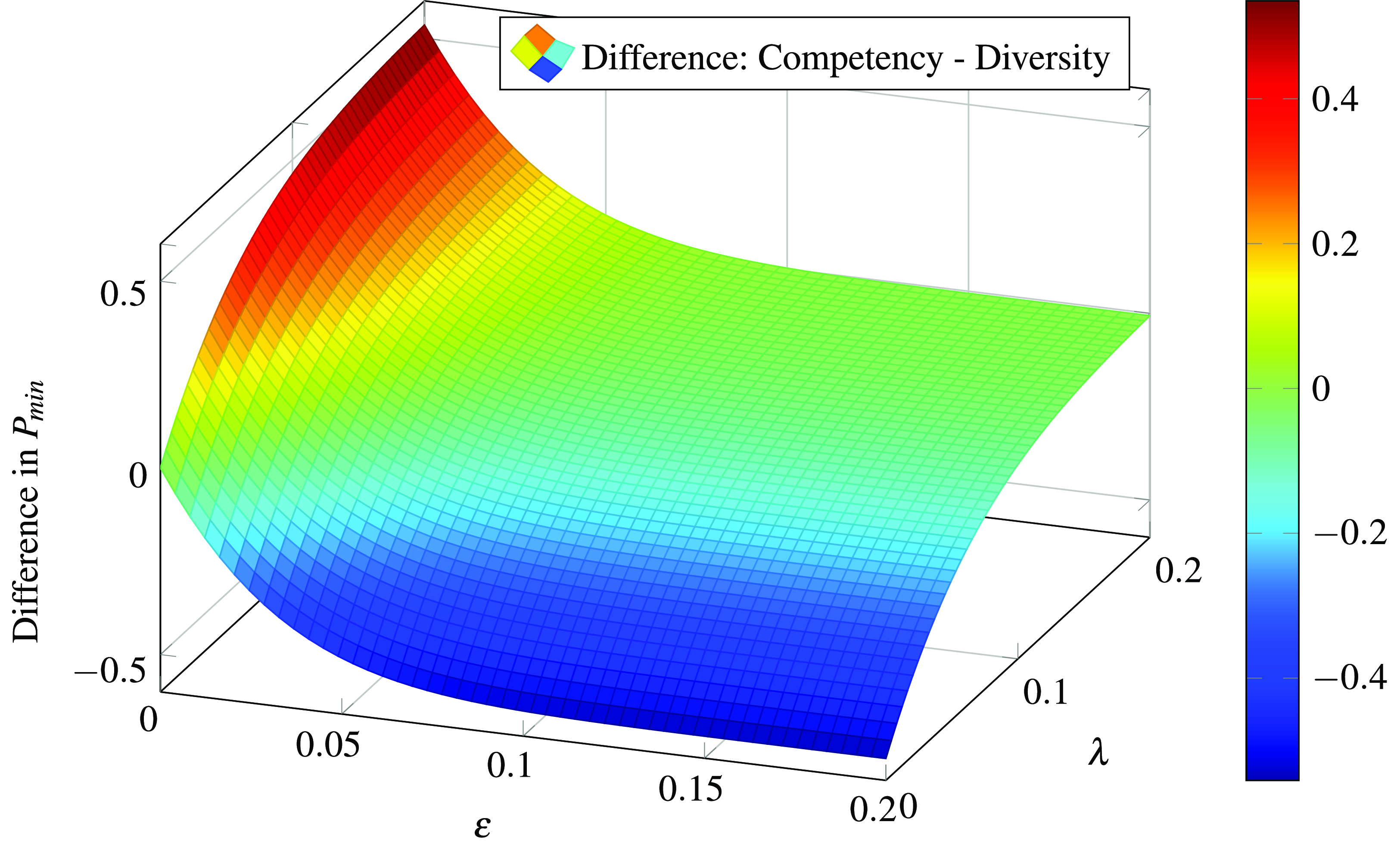
Figure 2. Difference in ${P_{min}}$
between the two functions as a function of
${P_{min}}$
between the two functions as a function of $\varepsilon $
and
$\varepsilon $
and $\lambda $
.
$\lambda $
.
Now that we have established a threshold for when diversity truly surpasses ability within the OL model, we turn to the next section to examine how this result fits within the broader research program of epistemic democracy and what contributions it offers to this field.
4 The bridge to epistemic democracy
In this section, we situate our results within the broader context of epistemic democracy. We begin with a brief overview of epistemic democracy and its long-standing connection to the CJT. Next, we summarize the CJT and its key generalizations. Finally, we revisit the DTA theorem and its implications for epistemic democracy.
To begin, what is epistemic democracy? Broadly speaking, it is a normative theory asserting that democratic institutions or procedures should track the truth to be considered legitimate (Dietrich and Spiekermann Reference Dietrich, Spiekermann, Knauff and Spohn2021). In this context, truth tracking refers to epistemic arguments that justify democratic institutions by assuming the existence of some objective truth about political matters – one that can be approximated through democratic processes (Holst and Molander Reference Holst and Molander2019).
4.1 Epistemic democracy and the CJT
As outlined in the introduction, a key result in the truth-tracking literature is the CJT, which provides probabilistic guarantees that, under specific assumptions, an electorate can correctly identify the best alternative through voting. This theorem is particularly relevant to epistemic democracy, as democratic institutions typically involve large groups of voters, thereby leveraging the wisdom of the crowds effect that underlies the CJT.
Analyzing democratic procedures from a truth-tracking perspective contrasts with their typical treatment in social choice theory, where voting rules are designed not to identify a correct alternative but to ensure equal treatment of all voters (Everaere et al. Reference Everaere, Konieczny, Marquis, Coelho, Studer and Wooldridge2010; Dietrich and Spiekermann Reference Dietrich, Spiekermann, Knauff and Spohn2021). Nonetheless, the epistemic democracy framework has a long-standing tradition in philosophical discourse.
According to Schwartzberg (Reference Schwartzberg2015), references to the wisdom of the crowds argument can be traced back to Aristotle, who stated:
There is this to be said for the many: each of them by himself may not be of a good quality; but when they all come together it is possible that they may surpass – collectively and as a body, although not individually – the quality of the few best, in much the same way that feasts to which many contribute may excel those provided at one person’s expense (Aristotle, Pol. 3.1281b).
Although generally skeptical of democratic ideals, Aristotle acknowledges a core principle of epistemic democracy: the epistemic advantage of collective deliberation. He argues that there is an epistemic benefit when notables and the populace deliberate together rather than when either deliberates alone (Bohman Reference Bohman2006). Unlike the CJT, however, Aristotle does not specify a precise mechanism – such as an opinion aggregation procedure – that could harness the epistemic benefits of the many (Bohman Reference Bohman2006). A first step in this direction can be found in Rousseau’s Social Contract (1762, see Gourevitch (Reference Gourevitch1997)), where he argues that through voting, people express their individual opinions, and the tally of these votes constitutes a declaration of the general will (Schwartzberg Reference Schwartzberg2015). Rousseau thus not only identifies a specific aggregation procedure – voting – but also specifies the truth to be tracked: the general will.
As noted by Schwartzberg (Reference Schwartzberg2015), it was Cohen’s (Reference Cohen1986) reinterpretation of Rousseau through the lens of the CJT that sparked renewed interest in epistemic democracy. This led to a substantial body of literature on the CJT and epistemic democracy, culminating in the observation that the CJT has been referred to as the “jewel in the crown of epistemic democrats” (List and Goodin 2001), as highlighted by Schwartzberg (Reference Schwartzberg2015). While the CJT’s importance to epistemic democracy is well established, it has also faced criticism (Schwartzberg Reference Schwartzberg2015). Estlund (Reference Estlund2008) argues that ’if democracy has any epistemic value, it is partly due to the sharing of diverse perspectives’. Consequently, the challenge of incorporating this diversity becomes paramount when employing the CJT to support democratic principles.
On the other hand, some scholars caution that an exclusive focus on diversity risks overlooking another key factor in democratic epistemic benefits: the role of experts (Holst and Molander Reference Holst and Molander2019). Specifically, it has been argued that insufficient attention has been given to how expertise can be leveraged to enhance the epistemic quality of democratic decision-making (Holst and Molander Reference Holst and Molander2019).
This leads to the first philosophical contribution of our results: we extend the long-standing discussion of the CJT in epistemic democracy by embedding formally precise definitions of diversity and expertise within the CJT framework. Specifically, we define a group as diverse if it has a low $\pi $
-value, indicating a low probability of following an opinion leader. Similarly, we characterize a group as highly expert if it has a large
$\pi $
-value, indicating a low probability of following an opinion leader. Similarly, we characterize a group as highly expert if it has a large ${\rm{\Delta }}p$
-value, representing a high average probability of selecting the correct alternative. Moreover, by introducing a diversity threshold, we formalize the interplay between diversity and expertise, allowing us to determine when one factor outweighs the other.
${\rm{\Delta }}p$
-value, representing a high average probability of selecting the correct alternative. Moreover, by introducing a diversity threshold, we formalize the interplay between diversity and expertise, allowing us to determine when one factor outweighs the other.
4.2 Generalizations of the CJT
To justify democratic procedures using the CJT, it is essential to develop generalizations that extend its core principles under more realistic conditions (Dietrich and Spiekermann Reference Dietrich, Spiekermann, Knauff and Spohn2021). Recall that the original CJT relies on several key assumptions: that all agents have equal competence (homogeneity), that they are more likely to select the correct alternative than an incorrect one (reliability), that their votes are cast independently, free from external influence (independence), and that they choose exactly one option (completeness) from a binary set of alternatives (dichotomy) in a majority vote.
In their seminal paper, Goodin and List (Reference List and Goodin2001) extend the original CJT to plurality voting, allowing agents to select a single alternative from a finite set – thus relaxing the dichotomy assumption. This contribution continues a long-standing tradition of adapting the CJT to more realistic settings. Subsequently, this result was further generalized by removing the completeness assumption, permitting agents to vote for multiple alternatives under approval voting (Everaere et al. Reference Everaere, Konieczny, Marquis, Coelho, Studer and Wooldridge2010).
Taking a different approach, Owen, Grofman, and Feld (Reference Owen, Grofman and Feld1989) demonstrated that the CJT holds even under heterogeneous competence levels, provided that independence, completeness, and dichotomy are maintained. In this setting, the only requirement is that, on average, agents are more likely to select the correct alternative than any other.
When allowing for interdependent voting choices, various models of dependence can be considered. A common approach introduces the concept of an opinion leader (OL), representing an external influence – such as extreme environmental conditions in sensor fusion scenarios or human actors like lobbyists and pundits in political debates.
Previous work on generalizing the CJT under the influence of an opinion leader began with Boland, Proschan, and Tong (Reference Boland, Proschan and Tong1989), who assumed homogeneous competence levels across agents and an equally competent OL in a dichotomous majority voting setting. Shortly after, Berg (Reference Berg1994) extended this framework to dichotomous weighted voting rules. Goodin and Spiekermann (Reference Spiekermann and Goodin2012) further generalized the dichotomous voting setting by allowing the OL’s competence to differ from that of the agents. Additionally, they identified a specific threshold at which the asymptotic behavior of the CJT fails.
As outlined in the preliminaries, a recent generalization of the CJT successfully relaxes all its original assumptions simultaneously (Karge et al. Reference Karge, Arisaka, Sanchez-Anguix, Stein, Aydoğan, van der Torre and Ito2024). This framework – underpinning the diversity threshold introduced in our study – permits agents to vote for any finite number of alternatives while accounting for heterogeneous competence levels and correlated voting behavior, modeled through an opinion leader. To the best of our knowledge, this represents the most general CJT result to date.
In essence, the CJT remains a foundational mechanism for justifying epistemic democracy (Schwartzberg Reference Schwartzberg2015), as it formalizes the wisdom of the crowds effect. The ongoing development of CJT research aims to maintain this core principle under increasingly realistic conditions that reflect actual electorates.
This leads to a second key contribution of our diversity results to the epistemic democracy literature. By being embedded within the most general CJT framework, it makes the least restrictive assumptions about the electorate. Furthermore, by providing a precise bound for when diversity outweighs expertise, it advances CJT research in its pursuit of identifying the exact conditions under which the wisdom of the crowds effect is preserved.
4.3 Epistemic democracy and DTA
Beyond the CJT, a second central mechanism in epistemic democracy – widely regarded as highly promising – is the DTA theorem (Schwartzberg Reference Schwartzberg2015). However, a key criticism of the DTA is that it fails to account for a fundamental epistemic challenge: it assumes that agents form their opinions independently, without external influences such as opinion leaders (Schwartzberg Reference Schwartzberg2015). In addition, it has often been recognized that democracies can benefit epistemically from diversity among their citizens, but that it is challenging why this is the case (Bohman Reference Bohman2006).
This brings us to our final contribution to the research program of epistemic democracy. We establish a formal connection between the two primary mechanisms that underpin the wisdom of the crowds effect – the CJT and the DTA – by embedding the DTA within the CJT framework. Moreover, by explicitly modeling the influence of an opinion leader, we provide a formal explanation for the epistemic benefits of diversity: specifically, its role in reducing systematic bias introduced by external influences.
5 Summarizing the argument and addressing key concerns
In this section, we summarize our main argument and address potential concerns. We began by noting that the original DTA theorem plays a significant role across various disciplines but has also faced substantial criticism regarding its mathematical rigor (Thompson Reference Thompson2014). Additionally, discussions of the DTA in decision-making typically revolve around three key epistemic frameworks: search problems, deliberation, and voting (Niesen et al. Reference Niesen, Spiekermann, Herzog, Girard and Vogelmann2024). Based on these observations, we can summarize our core argument as follows:
-
1. While the DTA is widely recognized for its significance, its mathematical foundations remain insufficiently rigorous. Thus, grounding it in a more robust mathematical framework is a worthwhile endeavor.
-
2. To ensure mathematical precision, we focus on one of the three primary epistemic frameworks – namely, voting.
-
3. Given that the CJT is the standard epistemic model for voting, we embed the DTA within the CJT framework, thereby clarifying the relationship between diversity and ability.
Building on these considerations, and our interpretation of diversity and ability within the CJT framework, we derived a mathematically precise bound that determines when diversity truly surpasses ability.
Potential Concerns. The structure of our argument is not without potential objections. Most notably, the CJT itself is subject to criticism. The original CJT relies on highly restrictive assumptions about the voting process – assumptions that are rarely met in practice. In particular, it presumes that voters are always more likely to choose the better of two alternatives and that their decisions are statistically independent. However, in reality, electorates often include incompetent or even malicious voters, and voting behavior is frequently correlated.
Given these limitations, one might raise the following concern: What justifies embedding an already debated theorem, the DTA, within another controversial framework, the CJT?
The response we have put forward in this paper is as follows: First, if we aim to make mathematically rigorous claims about the relationship between diversity and ability in voting, we must adopt a formal model of the voting process. This necessarily involves probabilistic assumptions about voters, which, like any model, require some level of abstraction from reality. Second, rather than embedding the DTA into the original, highly restrictive CJT, we incorporate it into a generalized version (Karge et al. Reference Karge, Arisaka, Sanchez-Anguix, Stein, Aydoğan, van der Torre and Ito2024), which, to our knowledge, is the least restrictive CJT framework available. Notably, this generalization accounts for unreliable agents and allows for correlations among voters, using the classical opinion leader model as established in the CJT literature.
A second line of criticism against the CJT and similar models of large elections has been raised by Barnett (Reference Barnett2020), who challenges the common assumption that large elections can be accurately modeled using a binomial framework. His argument suggests that this approach fails to capture important empirical patterns in election outcomes. To address this concern, we first outline the core of his critique.
Barnett’s Argument and the Binomial Model. In probabilistic models of large elections, it is common to assume a binomial structure, where each voter’s choice can be seen as an independent coin flip: each agent votes for a particular alternative with some probability, and does not vote for it otherwise.
Barnett (Reference Barnett2020) challenges this approach by arguing that it fails to explain a key empirical observation – large elections are frequently very close. If the binomial model were an accurate representation of voter behavior, it should naturally produce close elections under reasonable assumptions. However, Barnett constructs a simple counterexample demonstrating that when two candidates compete and one has even a slight advantage in voter preference, the probability of the less favored candidate winning rapidly approaches zero as the electorate grows. This suggests that, under the standard binomial model, competitive elections should be exceedingly rare, contradicting real-world patterns where close races are the norm. To illustrate his argument, Barnett (Reference Barnett2020) presents a small-scale counterexample:
Consider an election with two candidates, Donald and Daisy. Suppose each voter has a $50.5{\rm{\% }}$
probability of voting for Daisy, giving her only a slight advantage over Donald. Intuitively, we would expect the election to be relatively close, as the margin favoring Daisy is minimal. However, under the binomial model, the probability that Donald wins or ties the election is approximately 0.00000000000078 – less than one in a trillion (Barnett Reference Barnett2020). This stark contrast between the model’s prediction and our intuitive expectation highlights a potential flaw in using the binomial model to represent real-world elections.
$50.5{\rm{\% }}$
probability of voting for Daisy, giving her only a slight advantage over Donald. Intuitively, we would expect the election to be relatively close, as the margin favoring Daisy is minimal. However, under the binomial model, the probability that Donald wins or ties the election is approximately 0.00000000000078 – less than one in a trillion (Barnett Reference Barnett2020). This stark contrast between the model’s prediction and our intuitive expectation highlights a potential flaw in using the binomial model to represent real-world elections.
Let us assume that Barnett’s counterexample is valid and indeed challenges the binomial model as a framework for large elections. Even if we grant this, we argue that the underlying intuition behind his critique is not only unproblematic for our framework but actually reinforces it. While our model also represents an agent’s final vote as a probabilistic event – determined by a mixture of their private approval and the opinion leader’s choice – it crucially differs from the classical binomial model in one key aspect: the votes are not independent but correlated through the opinion leader.
By explicitly incorporating the opinion leader as a source of correlation, our model naturally accounts for the issue raised by Barnett. In fact, we can reformulate his counterexample within our framework as follows:
Example 6. Suppose we have two alternatives, $m = 2$
, and a total of
$m = 2$
, and a total of $n = 500,000$
agents. Each agent has a
$n = 500,000$
agents. Each agent has a $50.5{\rm{\% }}$
probability of voting for one alternative over the other, which corresponds to a
$50.5{\rm{\% }}$
probability of voting for one alternative over the other, which corresponds to a ${\rm{\Delta }}p$
-value of 0.01. Since there are only two alternatives, the probability of voting for the less favorable one is
${\rm{\Delta }}p$
-value of 0.01. Since there are only two alternatives, the probability of voting for the less favorable one is $1 - 0.505 = 0.495$
, and
$1 - 0.505 = 0.495$
, and ${\rm{\Delta }}p$
represents the difference between these probabilities. Now, assume that the opinion leader (OL) is as competent as the agents, meaning
${\rm{\Delta }}p$
represents the difference between these probabilities. Now, assume that the opinion leader (OL) is as competent as the agents, meaning $\hat p = 0.505$
, and that she exerts only minimal influence over the electorate, with each agent following the OL with a probability of just
$\hat p = 0.505$
, and that she exerts only minimal influence over the electorate, with each agent following the OL with a probability of just $1{\rm{\% }}$
. Applying Theorem 2, we can compute the minimal success probability for Daisy to win this election, which results in approximately 0.506, or just slightly above
$1{\rm{\% }}$
. Applying Theorem 2, we can compute the minimal success probability for Daisy to win this election, which results in approximately 0.506, or just slightly above $50{\rm{\% }}$
.
$50{\rm{\% }}$
.
This example demonstrates that by accounting for correlation among agents, our model not only avoids the flaw of the binomial model but also aligns with our intuition that the election should indeed be close.
6 Conclusion
In this paper, we brought together two foundational arguments in epistemic democracy: the DTA theorem and the CJT. By embedding the former within the framework of the latter, we provided a formal characterization of diversity and ability in voting contexts. This allowed us to derive a precise threshold for when diversity surpasses ability. Beyond establishing this result, we situated our findings within the broader discourse on epistemic democracy, highlighting its implications for the field. Finally, we addressed key concerns regarding our model.
We sincerely thank the two anonymous reviewers for their valuable feedback. In particular, we are grateful to the first reviewer for highlighting potential concerns regarding the structure of our argument and for drawing our attention to Barnett’s work (Reference Barnett2020). We also appreciate the second reviewer’s insightful suggestions on improving the presentation of key sections and their encouragement to provide a stronger philosophical motivation for our core results. This work is partly supported by BMBF in DAAD project 57616814 (SECAI).
Appendix A
A.1 Formal framework
Let $\;{\cal W} = \left\{ {{\omega _1}, \ldots, {\omega _m}} \right\}$
denote a finite set of
$\;{\cal W} = \left\{ {{\omega _1}, \ldots, {\omega _m}} \right\}$
denote a finite set of $m$
alternatives. Moreover, we define a finite set
$m$
alternatives. Moreover, we define a finite set ${\cal N} = \left\{ {{a_1}, \ldots, {a_n}} \right\}$
consisting of
${\cal N} = \left\{ {{a_1}, \ldots, {a_n}} \right\}$
consisting of $n$
agents. We can then represent a single approval voting (instance) by
$n$
agents. We can then represent a single approval voting (instance) by
 $$V \subseteq {\cal N} \times {\cal W}$$
where $\left( {{a_i},{\omega _j}} \right) \in V$
means that agent
$\left( {{a_i},{\omega _j}} \right) \in V$
means that agent ${a_i}$
approves choice
${a_i}$
approves choice ${\omega _j}$
. Subsequently, we define the score
${\omega _j}$
. Subsequently, we define the score ${\# _V}{\rm{\;}}\omega$
of some choice
${\# _V}{\rm{\;}}\omega$
of some choice $\omega \in {\cal W}$
as:
$\omega \in {\cal W}$
as:
 $${\# _V}{\rm{\;}}\omega = |\{ {a_i} \in {{\cal N}_n}|\left( {{a_i},\omega } \right) \in V\} |.$$
Finally, the winner of $V$
is defined to be the alternative that receives a strictly higher score than any alternative:
$V$
is defined to be the alternative that receives a strictly higher score than any alternative:
 $${\# _V}{\rm{\;}}\omega \gt \mathop {{\rm{max}}}\limits_{\omega {\rm{'}} \in {\cal W}\backslash \left\{ \omega \right\}} {\# _V}{\rm{\;}}\omega {\rm{'}}.$$
Example 7. Suppose we have $m = 3$
alternatives, i.e.,
$m = 3$
alternatives, i.e., $\;{\cal W} = \left\{ {{\omega _1},{\omega _2},{\omega _3}} \right\}$
and that we have
$\;{\cal W} = \left\{ {{\omega _1},{\omega _2},{\omega _3}} \right\}$
and that we have $n = 2$
agents, i.e.,
$n = 2$
agents, i.e., ${\cal N} = \left\{ {{a_1},{a_2}} \right\}$
. Suppose
${\cal N} = \left\{ {{a_1},{a_2}} \right\}$
. Suppose ${a_1}$
votes for the alternatives
${a_1}$
votes for the alternatives ${\omega _1},{\omega _2}$
and
${\omega _1},{\omega _2}$
and ${a_2}$
votes only for
${a_2}$
votes only for ${\omega _1}$
. Then
${\omega _1}$
. Then ${\omega _1}$
has a strictly higher score than either of the competing alternatives and wins the approval vote.
${\omega _1}$
has a strictly higher score than either of the competing alternatives and wins the approval vote.
The described voting scenario is modeled by a random process that generates the correct alternative, ${\omega _{\rm{*}}}$
, the OL’s choice as well as
${\omega _{\rm{*}}}$
, the OL’s choice as well as $V$
and is governed by a joint probability distribution
$V$
and is governed by a joint probability distribution $\mathbb P$
over the Bernoulli (i.e.,
$\mathbb P$
over the Bernoulli (i.e., $\left\{ {0,1} \right\}$
-valued) random variables
$\left\{ {0,1} \right\}$
-valued) random variables $X_{\rm{*}}^{{\omega _1}}, \ldots, X_{\rm{*}}^{{\omega _m}}$
,
$X_{\rm{*}}^{{\omega _1}}, \ldots, X_{\rm{*}}^{{\omega _m}}$
, $X_o^{{\omega _1}}, \ldots, X_o^{{\omega _m}}$
as well as
$X_o^{{\omega _1}}, \ldots, X_o^{{\omega _m}}$
as well as $X_i^{{\omega _1}}, \ldots, X_i^{{\omega _m}}$
for all agents
$X_i^{{\omega _1}}, \ldots, X_i^{{\omega _m}}$
for all agents $1, \ldots, i, \ldots, n$
and all alternatives
$1, \ldots, i, \ldots, n$
and all alternatives $1, \ldots, j, \ldots, m$
such that the values taken by these random variables represent the outcome of a voting event as follows.
$1, \ldots, j, \ldots, m$
such that the values taken by these random variables represent the outcome of a voting event as follows.
-
•
$X_{\rm{*}}^{{\omega _j}}$
is
$1$
if
${\omega _j}$
is the true world state (i.e.,
${\omega _j} = {\omega _{\rm{*}}}$
), else
$0$
, -
•
$X_o^{{\omega _j}}$
is
$1$
if the OL approves
${\omega _j}$
, and
$0$
otherwise, -
•
$X_i^{{\omega _j}}$
represents the private signal of the
$i$
th agent regarding his approval of the
$j$
th world state: it is
$1$
if
${a_i}$
privately approves
${\omega _j}$
and otherwise
$0$
.


Example 8. Suppose, as in the previous example, that we have $m = 3$
alternatives, i.e.,
$m = 3$
alternatives, i.e., $\;{\cal W} = \left\{ {{\omega _1},{\omega _2},{\omega _3}} \right\}$
and that we have
$\;{\cal W} = \left\{ {{\omega _1},{\omega _2},{\omega _3}} \right\}$
and that we have $n = 2$
agents, i.e.,
$n = 2$
agents, i.e., ${\cal N} = \left\{ {{a_1},{a_2}} \right\}$
. Let
${\cal N} = \left\{ {{a_1},{a_2}} \right\}$
. Let ${\omega _1}$
be the true state of the world, i.e.,
${\omega _1}$
be the true state of the world, i.e., ${X^{{\omega _1}}} = 1,{X^{{\omega _2}}} = 0,{X^{{\omega _3}}} = 0$
. The OL approves options 1 and 2, that is,
${X^{{\omega _1}}} = 1,{X^{{\omega _2}}} = 0,{X^{{\omega _3}}} = 0$
. The OL approves options 1 and 2, that is, $X_o^{{\omega _1}} = 1,X_o^{{\omega _2}} = 1,X_o^{{\omega _3}} = 0$
. Assume that
$X_o^{{\omega _1}} = 1,X_o^{{\omega _2}} = 1,X_o^{{\omega _3}} = 0$
. Assume that ${a_1}$
and
${a_1}$
and ${a_2}$
would vote as before if they were not influenced by the OL:
${a_2}$
would vote as before if they were not influenced by the OL: $X_1^{{\omega _1}} = 1,X_1^{{\omega _2}} = 1,X_1^{{\omega _3}} = 0,X_2^{{\omega _1}} = 1,X_2^{{\omega _2}} = 0,X_2^{{\omega _3}} = 0$
.
$X_1^{{\omega _1}} = 1,X_1^{{\omega _2}} = 1,X_1^{{\omega _3}} = 0,X_2^{{\omega _1}} = 1,X_2^{{\omega _2}} = 0,X_2^{{\omega _3}} = 0$
.
Given this joint distribution, we introduce the random variable $V_i^{{\omega _j}}$
, which represents the final outcome of an agent’s vote, i.e., after the OL’s potential influence. According to our assumption,
$V_i^{{\omega _j}}$
, which represents the final outcome of an agent’s vote, i.e., after the OL’s potential influence. According to our assumption, $V_i^{{\omega _j}}$
is the probabilistic mixture of
$V_i^{{\omega _j}}$
is the probabilistic mixture of $X_o^{{\omega _j}}$
with probability
$X_o^{{\omega _j}}$
with probability $\pi $
and of
$\pi $
and of $X_i^{{\omega _j}}$
with probability
$X_i^{{\omega _j}}$
with probability $1 - \pi $
. From this, we get for any
$1 - \pi $
. From this, we get for any $x \in \left\{ {0,1} \right\}$
that
$x \in \left\{ {0,1} \right\}$
that
 $${\mathbb P}V_i^{{\omega _j}} = x = \pi {\mathbb P}X_o^{{\omega _j}} = x + \left( {1 - \pi } \right){\mathbb P}X_i^{{\omega _j}} = x.$$
We denote by $p_1^\omega, \ldots, p_n^\omega $
the Bernoulli parameters of the “inner voice” random variables
$p_1^\omega, \ldots, p_n^\omega $
the Bernoulli parameters of the “inner voice” random variables $X_1^\omega, \ldots, X_n^\omega, $
for all
$X_1^\omega, \ldots, X_n^\omega, $
for all $\omega \in {\cal W}$
, that is,
$\omega \in {\cal W}$
, that is, $p_i^{{\omega _j}} = {\mathbb P}\left( {X_i^{{\omega _j}} = 1} \right)$
. In a similar vein, for every
$p_i^{{\omega _j}} = {\mathbb P}\left( {X_i^{{\omega _j}} = 1} \right)$
. In a similar vein, for every $\omega \in {\cal W}$
, we let
$\omega \in {\cal W}$
, we let ${\hat p^{{\omega _1}}}, \ldots, {\hat p^{{\omega _m}}}$
denote the Bernoulli parameters of the random variables
${\hat p^{{\omega _1}}}, \ldots, {\hat p^{{\omega _m}}}$
denote the Bernoulli parameters of the random variables $X_o^{{\omega _1}}, \ldots, X_o^{{\omega _m}}$
. Whether the OL approves the correct alternative, i.e., whether
$X_o^{{\omega _1}}, \ldots, X_o^{{\omega _m}}$
. Whether the OL approves the correct alternative, i.e., whether $X_o^{{\omega _{\rm{*}}}} = 1$
, is governed by the parameter,
$X_o^{{\omega _{\rm{*}}}} = 1$
, is governed by the parameter, $\hat p = {\mathbb P}\left( {X_o^{{\omega _{\rm{*}}}} = 1} \right)$
. For convenience, the choice of the correct alternative, or correct world state, being unknown to the agents, will be abbreviated by
$\hat p = {\mathbb P}\left( {X_o^{{\omega _{\rm{*}}}} = 1} \right)$
. For convenience, the choice of the correct alternative, or correct world state, being unknown to the agents, will be abbreviated by $\left[ {{\omega _{\rm{*}}}{ = _j}} \right]$
.
$\left[ {{\omega _{\rm{*}}}{ = _j}} \right]$
.
Example 9. We provide some example values for each parameter: Suppose that the OL has a rather high probability of approving the correct alternative $\hat p = 0.6$
and that agents are relatively inclined to follow the OL
$\hat p = 0.6$
and that agents are relatively inclined to follow the OL $\pi = 0.4$
. Suppose also that
$\pi = 0.4$
. Suppose also that ${a_1}$
has a high probability of voting for the first two alternatives when uninfluenced, but never votes for the third:
${a_1}$
has a high probability of voting for the first two alternatives when uninfluenced, but never votes for the third: $p_1^{{\omega _1}} = 0.8,p_1^{{\omega _2}} = 0.75,p_1^{{\omega _3}} = 0$
.
$p_1^{{\omega _1}} = 0.8,p_1^{{\omega _2}} = 0.75,p_1^{{\omega _3}} = 0$
.
In the following, we define the two central assumptions regarding the joint distribution. Conditioning upon the actual world state, we may define private agent approval independence as follows:
Definition 3 A joint distribution satisfies private agent approval independence if, conditioned on the actual world state, the private decision to approve any given ${\omega _j}$
is made independently across all agents, i.e., for any
${\omega _j}$
is made independently across all agents, i.e., for any $\omega, {\omega _j} \in {\cal W}$
and any sequence
$\omega, {\omega _j} \in {\cal W}$
and any sequence ${v_1}, \ldots, {v_n}$
of values from
${v_1}, \ldots, {v_n}$
of values from $\left\{ {0,1} \right\}$
the following holds:
$\left\{ {0,1} \right\}$
the following holds:
 $${\mathbb P}\mathop {\mathop \wedge \limits_{i = 1} }\limits^n X_i^{{\omega _j}} = {v_i}\left| {\left[ {{\omega _{\rm{*}}} = \omega } \right] = \mathop \prod \limits_{i = 1}^n {\mathbb P}X_i^{{\omega _j}} = {v_i}} \right|\left[ {{\omega _{\rm{*}}} = \omega } \right].$$
That is, conditional on the true state of the world, the joint probability of any given pattern of private approval decisions with respect to a given alternative can be computed by taking the product of the corresponding marginal probabilities.
Another central assumption concerns the “internal competence” $p_k^\omega $
of the
$p_k^\omega $
of the $k$
th agent regarding his ability to identify the true world state among any number of alternatives if no influence is exerted. This assumption can be formalized as follows, where we denote the average of these “internal competencies” with
$k$
th agent regarding his ability to identify the true world state among any number of alternatives if no influence is exerted. This assumption can be formalized as follows, where we denote the average of these “internal competencies” with
 $${\bar p^\omega } = {1 \over n}\mathop \sum \limits_{k = 1}^n p_k^\omega .$$
Definition 4 A joint probability distribution satisfies $\Delta p$
-group reliability for some
$\Delta p$
-group reliability for some $\Delta p \gt 0$
, if the probability, with respect to the agent’s inner voice, to approve the true world state, averaged across all agents, is at least by
$\Delta p \gt 0$
, if the probability, with respect to the agent’s inner voice, to approve the true world state, averaged across all agents, is at least by $\Delta p$
higher than the averaged probability for approving any other state, i.e., for every
$\Delta p$
higher than the averaged probability for approving any other state, i.e., for every $n$
and
$n$
and ${\omega _\dagger} \in {\cal W}\backslash \left\{ {{\omega _*}} \right\}$
holds
${\omega _\dagger} \in {\cal W}\backslash \left\{ {{\omega _*}} \right\}$
holds ${\bar p^{{\omega _*}}} \ge \Delta p + {\bar p^{{\omega _\dagger}}}.$
A.2 Proof of Theorem 4
Proof. The proof parallels that of Karge (Reference Karge, Burkhardt, Rudolph and Rusovac2024) for a similar case. Assume, $\pi = \bar \pi $
. Observe that both bounds are of the form
$\pi = \bar \pi $
. Observe that both bounds are of the form $1 - \left( {m - 1} \right)\left( {x + y} \right)$
where the factor
$1 - \left( {m - 1} \right)\left( {x + y} \right)$
where the factor $\left( {x + y} \right)$
of Theorem 3 and Theorem 2 respectively consist of two parts: one where the OL endorses the correct alternative, and one where this is not the case. Consider the first case in Theorem 3,
$\left( {x + y} \right)$
of Theorem 3 and Theorem 2 respectively consist of two parts: one where the OL endorses the correct alternative, and one where this is not the case. Consider the first case in Theorem 3, ${e^{ - {2 \over {4n}}{{(\Delta p\left( {\mathop \sum \nolimits_{k = 1}^s \left| {{{\cal G}_{{\pi _k}}}} \right|\left( {1 - {\pi _k}} \right)} \right))}^2}}})$
. By definition of
${e^{ - {2 \over {4n}}{{(\Delta p\left( {\mathop \sum \nolimits_{k = 1}^s \left| {{{\cal G}_{{\pi _k}}}} \right|\left( {1 - {\pi _k}} \right)} \right))}^2}}})$
. By definition of $\mathop \sum \nolimits_{k = 1}^s \left| {{{\cal G}_{{\pi _k}}}} \right|$
,
$\mathop \sum \nolimits_{k = 1}^s \left| {{{\cal G}_{{\pi _k}}}} \right|$
, $\mathop \sum \nolimits_{k = 1}^s \left| {{{\cal G}_{{\pi _k}}}} \right| = n$
. Moreover, by definition of
$\mathop \sum \nolimits_{k = 1}^s \left| {{{\cal G}_{{\pi _k}}}} \right| = n$
. Moreover, by definition of $\bar \pi $
,
$\bar \pi $
, $\mathop \sum \nolimits_{k = 1}^s {{\left| {{{\cal G}_{{\pi _k}}}} \right|} \over n}{\pi _k} = \bar \pi $
. Thus, as
$\mathop \sum \nolimits_{k = 1}^s {{\left| {{{\cal G}_{{\pi _k}}}} \right|} \over n}{\pi _k} = \bar \pi $
. Thus, as $\pi = \bar \pi $
by assumption,
$\pi = \bar \pi $
by assumption, $\mathop \sum \nolimits_{k = 1}^s {{\left| {{{\cal G}_{{\pi _k}}}} \right|} \over n}{\pi _k} = \pi $
.
$\mathop \sum \nolimits_{k = 1}^s {{\left| {{{\cal G}_{{\pi _k}}}} \right|} \over n}{\pi _k} = \pi $
.
Finally, $\mathop \sum \nolimits_{k = 1}^s \left| {{{\cal G}_{{\pi _k}}}} \right|\left( {1 - {\pi _k}} \right) = n\left( {1 - \pi } \right)$
when
$\mathop \sum \nolimits_{k = 1}^s \left| {{{\cal G}_{{\pi _k}}}} \right|\left( {1 - {\pi _k}} \right) = n\left( {1 - \pi } \right)$
when $\mathop \sum \nolimits_{k = 1}^s {{\left| {{{\cal G}_{{\pi _k}}}} \right|} \over n}{\pi _k} = \pi $
and
$\mathop \sum \nolimits_{k = 1}^s {{\left| {{{\cal G}_{{\pi _k}}}} \right|} \over n}{\pi _k} = \pi $
and $\mathop \sum \nolimits_{k = 1}^s \left| {{{\cal G}_{{\pi _k}}}} \right| = n$
.
$\mathop \sum \nolimits_{k = 1}^s \left| {{{\cal G}_{{\pi _k}}}} \right| = n$
.
As ${\rm{\Delta }}p$
is fixed, we have that
${\rm{\Delta }}p$
is fixed, we have that ${({\rm{\Delta }}p\left( {\mathop \sum \nolimits_{k = 1}^s \left| {{{\cal G}_{{\pi _k}}}} \right|\left( {1 - {\pi _k}} \right)} \right))^2} = {(n\left( {1 - \pi } \right){\rm{\Delta }}p)^2}$
.
${({\rm{\Delta }}p\left( {\mathop \sum \nolimits_{k = 1}^s \left| {{{\cal G}_{{\pi _k}}}} \right|\left( {1 - {\pi _k}} \right)} \right))^2} = {(n\left( {1 - \pi } \right){\rm{\Delta }}p)^2}$
.
By algebra, we obtain ${e^{ - {2 \over {4n}}{{({\rm{\Delta }}p\left( {\mathop \sum \nolimits_{k = 1}^s \left| {{{\cal G}_{{\pi _k}}}} \right|\left( {1 - {\pi _k}} \right)} \right))}^2}}}) = {e^{ - {1 \over 2}n{\rm{\Delta }}{p^2}{{(1 - \pi )}^2}}}$
. As an analogous argument can be made for the subcase where the OL is wrong, we conclude that
${e^{ - {2 \over {4n}}{{({\rm{\Delta }}p\left( {\mathop \sum \nolimits_{k = 1}^s \left| {{{\cal G}_{{\pi _k}}}} \right|\left( {1 - {\pi _k}} \right)} \right))}^2}}}) = {e^{ - {1 \over 2}n{\rm{\Delta }}{p^2}{{(1 - \pi )}^2}}}$
. As an analogous argument can be made for the subcase where the OL is wrong, we conclude that ${P_{min,\pi }} = {P_{min,\bar \pi }}$
.
${P_{min,\pi }} = {P_{min,\bar \pi }}$
.
A.3 Proof of Corollary 1
The proof is similar to a proof for a similar problem in Karge (Reference Karge, Arisaka, Sanchez-Anguix, Stein, Aydoğan, van der Torre and Ito2024).
Proof. To determine this threshold, we introduce the parameter $\varepsilon $
, which represents the amount by which the average correlation is smaller in the more diverse group. Similarly,
$\varepsilon $
, which represents the amount by which the average correlation is smaller in the more diverse group. Similarly, $\lambda $
represents the increase in competency in the less diverse group. The more diverse group outperforms the more competent one as soon as the minimal success probability is greater, that is, as soon as:
$\lambda $
represents the increase in competency in the less diverse group. The more diverse group outperforms the more competent one as soon as the minimal success probability is greater, that is, as soon as:
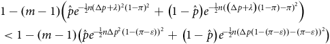 $$\eqalign{
& 1 - \left( {m - 1} \right)\left( {\hat p{e^{ - {1 \over 2}n{{(\Delta p + \lambda )}^2}{{(1 - \pi )}^2}}} + \left( {1 - \hat p} \right){e^{ - {1 \over 2}n{{(\left( {\Delta p + \lambda } \right)\left( {1 - \pi } \right) - \pi )}^2}}}} \right) \cr
& < 1 - \left( {m - 1} \right)\left( {\hat p{e^{ - {1 \over 2}n\Delta {p^2}{{(1 - \left( {\pi - \varepsilon } \right))}^2}}} + \left( {1 - \hat p} \right){e^{ - {1 \over 2}n{{(\Delta p\left( {1 - \left( {\pi - \varepsilon } \right)} \right) - \left( {\pi - \varepsilon } \right))}^2}}}} \right) \cr} $$
$$\eqalign{
& 1 - \left( {m - 1} \right)\left( {\hat p{e^{ - {1 \over 2}n{{(\Delta p + \lambda )}^2}{{(1 - \pi )}^2}}} + \left( {1 - \hat p} \right){e^{ - {1 \over 2}n{{(\left( {\Delta p + \lambda } \right)\left( {1 - \pi } \right) - \pi )}^2}}}} \right) \cr
& < 1 - \left( {m - 1} \right)\left( {\hat p{e^{ - {1 \over 2}n\Delta {p^2}{{(1 - \left( {\pi - \varepsilon } \right))}^2}}} + \left( {1 - \hat p} \right){e^{ - {1 \over 2}n{{(\Delta p\left( {1 - \left( {\pi - \varepsilon } \right)} \right) - \left( {\pi - \varepsilon } \right))}^2}}}} \right) \cr} $$
Instead of determining the threshold for the general case, we observe that increasing $\pi $
has the most detrimental effect on the group’s ability to identify the correct alternative when
$\pi $
has the most detrimental effect on the group’s ability to identify the correct alternative when $\hat p$
is low. In the worst case,
$\hat p$
is low. In the worst case, $\hat p = 0$
. Therefore, to derive the desired threshold for when an increase in diversity outweighs an increase in competence for the competing group, we consider this worst case and assume
$\hat p = 0$
. Therefore, to derive the desired threshold for when an increase in diversity outweighs an increase in competence for the competing group, we consider this worst case and assume $\hat p = 0$
. In this scenario, the above expression simplifies to
$\hat p = 0$
. In this scenario, the above expression simplifies to
 $$1 - \left( {m - 1} \right){e^{ - {1 \over 2}n{{(\Delta p + \lambda \left( {1 - \pi } \right) - \pi )}^2}}} \lt 1 - \left( {m - 1} \right){e^{ - {1 \over 2}n{{(\Delta p\left( {1 - \left( {\pi - \varepsilon } \right)} \right) - \pi - \varepsilon )}^2}}}$$
We further simplify this problem by noting that the two expressions differ only in their exponents. Since they are of the form ${e^{ - x}}$
and
${e^{ - x}}$
and ${e^{ - y}}$
, respectively, they increase as
${e^{ - y}}$
, respectively, they increase as $x$
and
$x$
and $y$
decrease. With an increasing factor of the form
$y$
decrease. With an increasing factor of the form ${e^{ - x}}$
, the total expression of the form
${e^{ - x}}$
, the total expression of the form $1 - \left( {m - 1} \right){e^{ - x}}$
increases, and so does the minimum probability of success.
$1 - \left( {m - 1} \right){e^{ - x}}$
increases, and so does the minimum probability of success.
For the sake of simpler algebra, we check for when
 $$ - {1 \over 2}n{(\Delta p + \lambda \left( {1 - \pi } \right) - \pi )^2} \lt - {1 \over 2}n{(\Delta p\left( {1 - \pi - \varepsilon } \right) - \pi - \varepsilon )^2}$$
By solving for $\varepsilon $
, we can derive that this inequality is true if
$\varepsilon $
, we can derive that this inequality is true if
 $$\varepsilon \lt {{\lambda - \pi \lambda } \over {\Delta p + 1}}$$
From this, we can derive that
 $$1 - \left( {m - 1} \right){e^{ - {1 \over 2}n{{({\rm{\Delta }}p + \lambda \left( {1 - \pi } \right) - \pi )}^2}}} \lt 1 - \left( {m - 1} \right){e^{ - {1 \over 2}n{{({\rm{\Delta }}p\left( {1 - \pi - \varepsilon } \right) - \pi - \varepsilon )}^2}}}$$
if
 $$\varepsilon \ge {{\lambda - \pi \lambda } \over {{\rm{\Delta }}p + 1}}$$


 Open access