Determination of cavitation zone for cavitating waterjet machining using numerical simulation

Abstract

Recent developments of non-traditional machining techniques, like cavitating waterjet machining (CWJM), have gained attention for their simple operation and environment friendliness with zero carbon footprints. Cavitating waterjet machining leverages the erosive power of cavity bubbles combined with a waterjet to machine or modify a workpiece. For effective CWJM, proper positioning of the workpiece is crucial. The implosion of cavity bubbles generates microjets and shock waves, creating high temperatures and pressures for a few microseconds, impacting the workpiece. This study numerically and analytically investigates the cavitation phenomenon and their effects. Numerical simulation employs an implicit finite volume scheme with the Semi-Implicit Method for Pressure Linked Equations (SIMPLE) algorithm solving Reynolds-averaged Navier–Stokes equations. It also incorporates a discrete phase model (DPM) to analyse bubble distribution and size. An analytical model calculates the hydrodynamic impact load on the workpiece. The study measures hydrodynamic stress and microjet velocities from bubble implosions, using reverse engineering to assess cavitation impact on ductile materials (aluminium and chromium steel). The result reveals a linear relationship between pit deformation and hydrodynamic impact, with impacts ranging from 200 to 1000 MPa, and microjet velocities between 100 and 800 m s⁻¹. Finally, this work accurately predicts the standoff distance and cavitation intensity in the downstream of flow domain.

Impact Statement

The research addresses the challenge of optimising cavitating water jet machining (CWJM), a sustainable and non-traditional machining process that leverages cavitation bubbles for material removal. Despite its growing significance due to environmental benefits, current studies lack a comprehensive understanding of the cavitation zone, standoff distance and material interaction during machining. This research fills that gap by conducting numerical simulations to determine the optimal standoff distance and cavitation zone, improving machining precision and efficiency. The findings help identify the correct positioning of workpieces for both material removal and surface treatment, enhancing the process’s effectiveness while minimising experimental trial and error. This advancement in CWJM has the potential to increase its adoption in industries, offering a cleaner and more cost-effective alternative to conventional machining methods, thus contributing to more sustainable manufacturing practices.

1. Introduction

Cavitation in a continuous and homogeneous liquid medium occurs when the local pressure drops below the vapour pressure of the liquid at constant temperature, causing the formation of cavitating bubbles. These bubbles collapse or implode, generating shock waves and high-intensity pressure waves in the local region. They have detrimental effects on the performance and efficiency of mechanical devices, such as pumps, turbines and propellers causing erosion, noise and vibrations. The synergistic effects of cavitation erosion can also be used for removing oxide and paint layers, machining complex and intricate parts and performing surface treatment (Kim et al., 2014; Kubota et al., 1992). The cumulative effect of cavitation in association with a high-speed waterjet can be exploited for material removal and surface modification. When the cavitation phenomenon is used for material removal from the target surface, the process is commonly known as cavitating waterjet machining (CWJM). While it is used for surface treatment or modification of an object, the process is called cavitating waterjet peening (CWJP). Both CWJM and CWJP are environmentally benign processes that produce negligible pollutants, carbon footprints contributing to sustainable machining and cleaner production systems to a large extent.

Cavitating waterjet machining is a non-traditional machining technique that involves the use of cavitation phenomenon to remove undesirable material from a workpiece. It utilises the erosive power of cavitating bubbles to erode or remove material from a workpiece. The process typically involves the use of a high-pressure liquid to generate and control the cavity bubbles impinging on the workpiece’s surface and causing localised erosion (Karimi and Avellan, 1986). In addition to material removal, CWJP can be used for the surface treatment of materials depending upon cavitation intensity. The cavitation intensity depends on many shockwaves and micro-jets that induce compressive residual stresses and plastic deformation of material. Thus, it improves the fatigue strength, wear resistance and surface integrity of metallic components (Soyama, 2007; Soyama et al., 2001). Although CWJM and CWJP are cavitation related phenomena, the cavitation zone for CWJM and CWJP ,where the target workpiece is placed for processing, is different depending upon cavitation intensity. To improve the machining performance and efficiency, identifying the proper cavitation zone in the cavitation chamber either for machining or peening operations is essential, and computational investigation is essential before conducting actual experiment. Therefore, the present work investigates the CWJM process based on liquid properties, jet pressure, velocity and standoff distance.

During the CWJM process, the workpiece surface is subjected to a cavitating jet for material erosion. In this process, the behaviour of cavitation in a flow domain is difficult to understand experimentally as there are a lot of complex fluid phenomena that exist such as multiple phase transition, turbulence and their interactions (Pendar et al., 2020). Therefore, computational investigations on cavitation phenomenon with jet formation in a flow domain are required in comprehending the CWJM process to a great extent. Due to the above difficulty in realising the exact zone where the cavitation phenomenon occurs during material processing, a computational fluid dynamics (CFD) model is used and the flow behaviour inside and at the exit of the orifice are simulated in the present work.

1.1. Literature review

The computational modelling of cavitation phenomenon can be done majorly in two ways, namely the volume of fluid (VOF) method based on interface tracking and the homogeneous mixture model based on phase interaction. The homogeneous mixture model is more popular due to its computational inexpensiveness as compared with the VOF method. There are many cavitation models based on the homogeneous mixture model, such as those developed by Kunz et al. (Kunz et al., 2000), Schnerr and Saur (Schnerr and Sauer, 2001) and Singhal et al. (Singhal et al., 2002). In the homogeneous mixture model method, the model treats the phases as a continuous medium for the liquid and vapour phases respectively and couples both set of equations. Zhao et al. (Zhao et al., 2011) conducted numerical simulations of cavitation flow on a NACA0015 hydrofoil under high-pressure and high-temperature conditions. The simulations utilised a homogeneous mixture model in conjunction with the cavitation mass transfer model proposed by Singhal et al. (Singhal et al., 2002) to accurately predict hydrodynamic cavitation. Guoyi et al. (Guoyi et al., 2011) presented a practical compressible mixture flow model for simulating turbulent cavitating flows in high-speed waterjets. By coupling a simplified estimation of bubble cavitation with a compressible mixture flow computation based on unsteady Reynolds-averaged Navier-Stokes (URANS), the study accurately predicts cavitation behaviour in a submerged waterjet. They concentrated on initial occurrence of cavitation at the orifice entrance, the downstream expansion and shedding of bubble clouds, and the impact of cavitation bubbles on the flow velocity. Basir et al. (Bashir et al., 2011) investigated hydrodynamic cavitation behaviour in a different venturi design based on the model proposed by Singhal et al. (Singhal et al., 2002). Kuldeep and Saharan (Kuldeep and Saharan 2016) explored a computational study on the optimisation of different geometrical parameters of two types of hydrodynamic cavitation reactors, namely venturi type and orifice type. The study focuses on the inception, growth and dynamics of cavities in these reactors. They found that, for venturi-type reactors, a throat diameter-to-length ratio of 1:1 and a divergence angle of 6.5° are optimal for cavitation phenomenon. Similarly, for orifice-type reactors, a diameter-to-length ratio of 1:3 and an increase in the total flow area result in increased cavitation activity. Simpson and Ranade (Simpson and Ranade, 2018) explored the behaviour of cavitation phenomenon in the different orifice and venturi design considering the homogeneous mixture model. Kubota et al. (Kubota et al., 1992) developed a model for cavitating flows considering the cavitation cloud as a homogeneous cluster of spherical bubbles, and the rate of change of bubble radius is calculated by the Rayleigh–Plesset–Poritsky equation. Sonde et al. (Sonde et al., 2018) studied cavitation peening using CFD based on the Schnerr and Saur (SS) cavitation mass transfer model along with a k − ε realisable turbulence model. It is concluded that the collapse of cavity bubbles generates mechanical loading on the surface which leads to generation of compressive residual stresses. Kozak et al. (Kozák et al., 2019) performed a numerical study on cavitating flow in a venturi tube using a multiphase VOF method with the k − ε turbulence model to complement the experimental results. In their study, they highlighted that the CFD results can provide much more insight into the hydrodynamic effect of flow like velocity fields, swirl effect, pressure loss and the cavitating vortex structure. Ji et al. (Ji et al., 2024) carried out a comprehensive review of CFD methods on modelling of cavitation phenomenon, considering various approaches like the Euler–Euler and Euler–Lagrangian approaches. Wang et al. (Wang et al., 2021) simulated unsteady cavitating turbulent flow around a Clark-Y hydrofoil using the Eulerian–Lagrangian approach with large eddy simulations in conjunction with the SS cavitation model. It reveals the role of the re-entrant jet in the bubble dynamics, and its impact on the bubble size distribution. Wang et al. (Wang et al., 2023) presented a numerical investigation of cloud cavitating flow around a Delft Twist-11 hydrofoil using a multiscale Euler–Lagrange approach. It depicts the evolution of U-shaped cavitation structures into microbubble clouds and detects dual bubble size spectra impacted by shear layers and vortex-induced growth, like breaking ocean waves. Recently, Kumar et al. (Kumar et al., 2024) investigated cavitation phenomenon, including the aspect ratio of the orifice, bubble statistics and the dynamics of cavity bubbles. However, they did not address the cavitating jet velocity and standoff distance to harness the combined effects of the waterjet and cavity bubbles. So far, there is a very little work on the identification of the cavitation zone in the cavitation chamber to place the workpiece for machining and peening along with various process parameters such as pressure distribution, high volume fraction of vapour, velocity of jet, etc.

In order to study the pressure gradient and phase interaction inherent in the cavitation phenomenon, an appropriate turbulence model is essential. Yuan et al. (Yuan et al., 2001) have performed CFD simulation of cavitation phenomenon using a k − ω turbulence model including growth and collapse of cavity bubbles inside the nozzle. Deng et al. (Deng et al., 2009) carried out the numerical simulation of the cavitating flow with a nozzle angle adopting a k − ε turbulence model using Fluent software and verified the simulated results with experimentation. Zhang et al. (Zhang et al., 2013) carried out the numerical simulation on cavitation behaviour in the water cavitation peening process with the Renormalization group (RNG) k − ε turbulence model including the velocity and vapour fraction inside and outside of the nozzle in the flow domain. To accurately compute the turbulent flow at the exit of the orifice, the realisable k − ε turbulence model with standard wall functions is employed.

Understanding the wide range of impact loads generated by cavitation is crucial for assessing the aggressiveness of fluid flow and the resulting material erosion. Traditionally, this information has been obtained using conventional pressure sensors (Franc and Michel, 1997; Hattori and Takinami, 2010). Previous research has explored various techniques, such as utilising piezoelectric film pressure transducers, magnesium oxide crystals and ceramic pressure transducers, to measure the implosion pulses of cavity bubbles (Franc and Michel, 1997; Momma and Lichtarowicz, 1995; Okada et al., 1995). However, due to limitations related to rise time, resonant frequency and sensor placement, these methods may not provide precise measurements of the impact loads from bubble implosions. To address these challenges, Carnelli et al. (2012b, Carnelli et al., 2012a) proposed a novel approach using materials themselves as sensors. This reverse engineering technique involves measuring the stresses and hydrodynamic impacts resulting from the implosion of cavity bubbles. By analysing the material’s response to these impacts, this method offers a more accurate and insightful means of quantifying the forces during cavitation events.

1.2. Research gap, problem statement, objectives, and novelty of work

Through an extensive literature review, no computational works were found that address the standoff distance and the region where the CWJM and CWJP will be effective. In CWJM, the implosion of a bubbles and speed of the microjet are the primary sources of energy for material removal. Thus, the process to produce cavity bubbles for CWJM is essential, and the associated parameters such as material properties, fluid properties, velocity of microjet and location of workpiece in the cavitation process are still untouched and need further investigation to accelerate the process of cavitating waterjet machining and peening. The placement of the workpiece and standoff in the CWJM is rarely discussed numerically in the literature. Therefore, to bridge the above-described gaps the present study discusses an attempt to improve the effectiveness of the CWJM process.

The work is presented in following ways. All the governing equations and numerical models used for CWJM and CWJP are presented in section 2. The numerical simulation with model validation and computational findings are discussed in section 3. Finally, the critical findings of the present study are concluded along with answers to the research questions and concluded in section 4.

2. Numerical modelling

An orifice plate in a flow domain is used to generate a hydrodynamic cavitating waterjet. In this study, a multiphase CFD model has been used to simulate cavitating flow with necessary boundary conditions. The schematic diagram with design features of the flow domain and orifice plate that induce cavity bubble is presented in Figure 1.

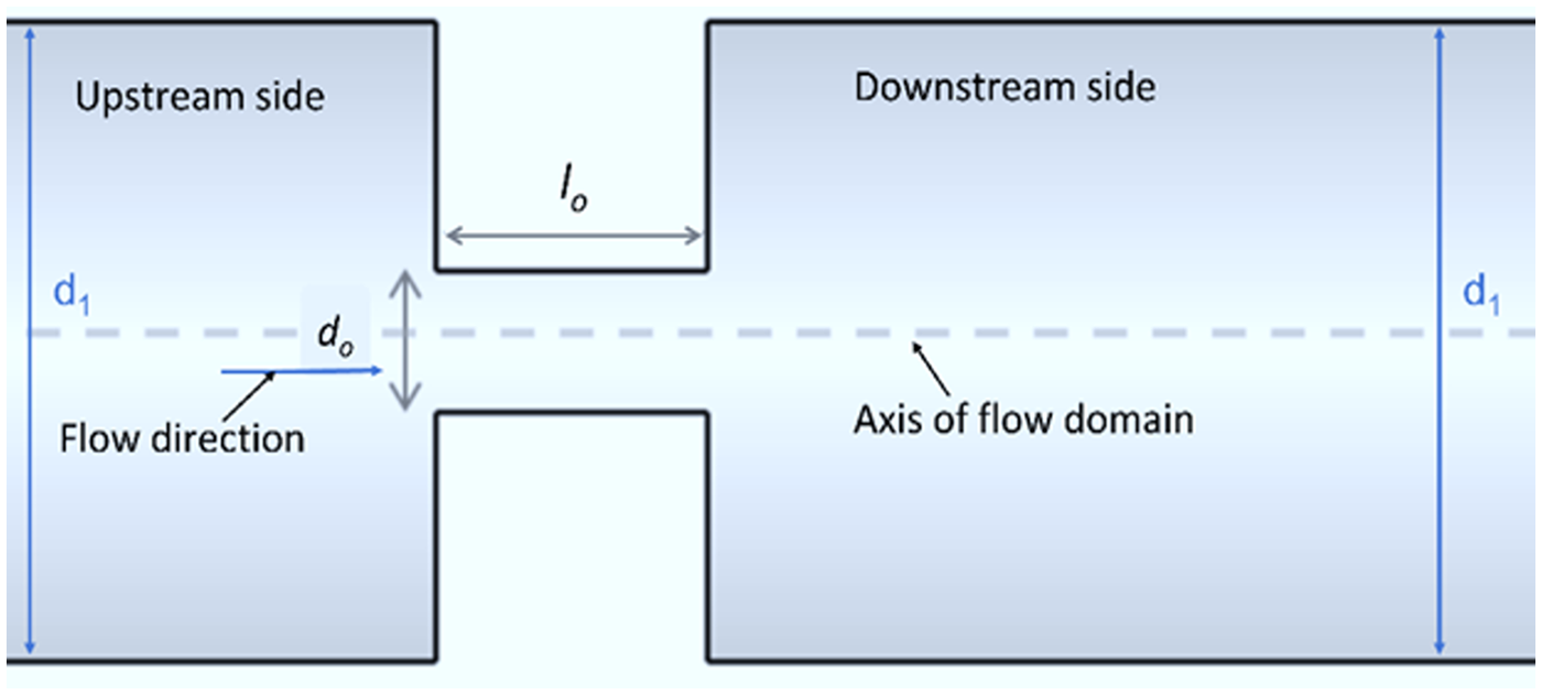
Figure 1. Schematic representation of computational fluid field with an orifice.

The length (l _o ) and diameter (d _o ) of the orifice plate are as shown in Figure 1. The present investigation aims to:

1. a. Determine the effective standoff distance for a cavitating waterjet to enhance the impact of a waterjet with cavitation.

2. b. Determine the precise location of the specimen to achieve cavitating waterjet peening and machining in the CWJM process.

3. c. To determine the hydrodynamic impact pressure required to create pits using the inverse finite element method approach in CWJM.

To describe the detailed course of action of the computational investigation of CWJM, a flow chart is presented in Figure 2. Each block in the figure represents the steps followed with the order.

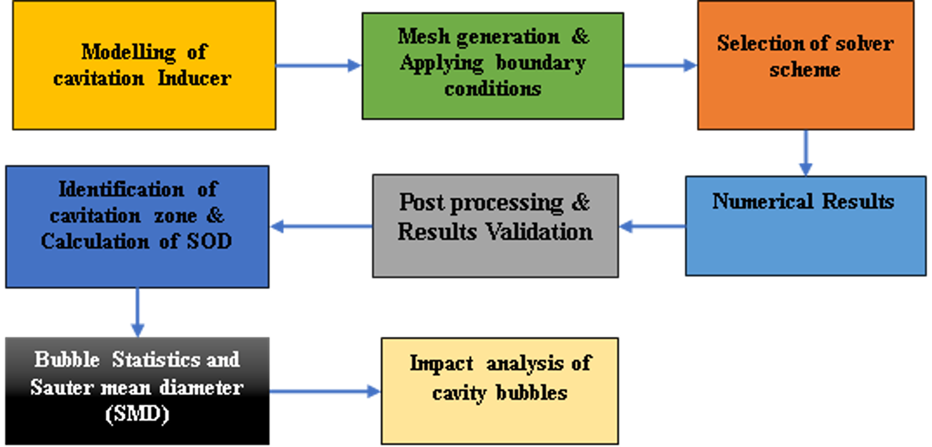
Figure 2. Flow chart for numerical modelling.

2.1. Cavity bubble inception

The fluid flowing through a contraction, result in the separation of the boundary layer and a substantial increase in velocity, accompanied by a turbulent field. The turbulence intensity significantly influences cavitation activity and its severity. Equation (2.1) presents a dimensionless number referred as cavitation number (CN), which quantifies the severity of cavitation within the flow domain

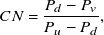(2.1) \begin{align} CN=\frac{P_{d}-P_{v}} {P_{u}-P_{d}}, \end{align}

where P _d and P _v are the recovered downstream pressure and vapour pressure of the liquid at constant temperature, respectively, P _u is the upstream pressure in fluid domain. The CN provides the intensity of cavitation phenomenon in the fluid domain due to a contraction in flow geometry which leads to an increase in the velocity of the flow lamina. The higher pressure gradient across the flow domain results in a lower value of CN, which means more inception of the cavity bubbles and higher chances of material removal (Mehdi Hadi, 2013). Thus, the cavity bubble initiation occurs at CN <1. The governing equation and mathematical formulation to simulate the fluid flow and cavitation phenomenon are described further.

2.2. Turbulence model

In this section the governing models for a homogeneous multiphase (water and vapour) cavitating waterjet through an orifice are discussed. A realisable k − ε turbulence model with standard wall function is used. This model, based on Reynolds-averaged NavierStokes (RANS) equations, effectively addresses mathematical instability inherent in highly turbulent flows. In the present study, the homogeneous mixture of water and vapour is considered as a single fluid. Consequently, the homogeneous mixture fluid is appropriately coupled to mass transfer equations. The primary governing equations, along with the turbulence model for CFD simulation, are elaborated in the subsequent sub-section. The continuity equation of homogeneous mixture is expressed in equation (2.2)

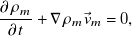(2.2) \begin{align} \frac{\partial \rho _{m}} {\partial t}+\nabla \rho _{m} \vec {v}_{m}=0, \end{align}

where ρ _m and $ \vec {v}_{m} $ are the density and velocity of the mixture phase, respectively. Assuming both phases flow at the same velocity, the momentum equation for the homogeneous mixture fluid is given in equation (2.3)

(2.3) \begin{align}\frac {\partial \left(\rho _{m}\vec {v}_{m}\right)}{\partial t}+\nabla \cdot \left(\rho _{m}\vec {v}_{m}\vec {v}_{m}\right)=-\nabla p+\nabla \cdot \left[\mu _{m}(\nabla \vec {v}_{m}+\nabla {\vec {v}_{m}}^{T})\right]+\rho _{m}\overset{\tiny\rightharpoonup}{g}+\overset{\tiny\rightharpoonup}{F}, \end{align}

where μ _m is the viscosity of the mixture fluid, $ \rho_{m} \overset{\tiny\rightharpoonup}{g} $ is the gravitational body force and the term $ \overset{\tiny\rightharpoonup}{F} $ accounts for the added body forces applied to the mixture fluid volume (this force may arise from the interaction with a secondary phase). Therefore, the Boussineq hypothesis (Guide, 2013) is used to close the RANS equation. In addition, k is the turbulence kinetic energy and ε is the turbulence dissipation rate which are modelled using the transport equations (2.4)–(2.5)

(2.4) \begin{align} & \frac {\partial}{\partial t}\left(\rho k\right)+ \frac{\partial}{\partial x_{i}}\left(\rho kv_{i}\right)= \frac{\partial}{\partial x_{i}}\left(\Gamma _{k} \frac{\partial k }{\partial x_{i}}\right)+G_{k}-G_{b}-\rho \varepsilon -Y_{k}+S_{k}, \end{align}

(2.5) \begin{align} & \frac{\partial}{\partial t}\left(\rho \varepsilon \right) + \frac{\partial}{\partial x_{i}}\left(\rho \varepsilon v_{i}\right) = \frac{\partial }{ \partial x_{i}}\left(\Gamma _{\varepsilon } \frac{\partial \varepsilon }{\partial x_{i}}\right)+\rho C_{1}S\varepsilon -\rho C_{2} \frac{\varepsilon ^{2}}{k+\sqrt{\nu \varepsilon }}+C_{1\varepsilon } \frac{\varepsilon}{k}C_{3\varepsilon }G_{b}+S_{\varepsilon }, \\[10pt] \nonumber \end{align}

where $C_{1}=\mathit{\max } \left[0.43, \frac{\eta }{\eta +5}\right],\eta =S \frac{k }{\varepsilon },S=\sqrt{2S_{ij}S_{ij}}$

In equations (2.4)-(2.5), G _k is the initiation of k due to the mean velocity gradient. G _b is used for the generation of k due to the buoyancy effect. However, in the present study the buoyancy effect on ε is neglected, by placing the value of G _b to zero in equation (2.5). Also, Γ _k and Γ _ε represent the effective diffusivity of k and ε, respectively, Y _k is the dissipation of k due to turbulence, C ₂ and C _1ε are constant values of 1.9 and 1.44, respectively (Guide, 2013), and S _k and S _ε are user defined source terms. The cavitation model is discussed in the following sub-section.

2.3. Cavitation model

The cavitation model proposed by Schnerr and Sauer (Schnerr and Sauer, 2001) has been used in the present study. This model helps in determining flow properties of the mixture fluid as a linear function of vapour volume fraction. Therefore, the density of the mixture fluid is shown in equation (2.6)

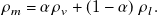(2.6) \begin{align} \rho _{m}=\alpha \rho _{v}+\left(1-\alpha \right)\rho _{l}. \end{align}

The liquid–vapour mass transfer occurs in the limited zone for incompressible homogeneous mixture flow, when the static pressure is lower than or equal to the vapour pressure at constant temperature of the working fluid. The vapour transport equation that governs the mass transfer between liquid and vapour is given in equation (2.7)

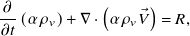(2.7) \begin{align} \frac {\partial}{\partial t}\left(\alpha \rho _{v}\right)+\nabla \cdot \left(\alpha \rho _{v}\vec {V}\right)=R, \end{align}

where α stands for vapour fraction, ρ _v stands for density of the vapour phase, $ \vec{V} $ is the velocity. Equation (2.8) shows the net mass source term R from the liquid to vapour

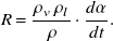(2.8) \begin{align} R= \frac{\rho _{v}\rho _{l}}{\rho }\cdot \frac{d\alpha}{dt}. \end{align}

The cavitation models considered in the present research are derived based on various assumptions such as the mixture is supposed to be incompressible and homogeneous; the nuclei that already exist in the flow regime are the source for the cavity bubble, which can grow and implode depending on the surrounding conditions (temperature and pressure); the slip velocity between the phases is neglected; positive mass transfer from liquid to vapour is considered; and the bubble growth is represented by a simplified Rayleigh–Plesset equation.

Nonetheless, the carrier fluid contains a large number of nuclei that are needed for the cavity bubble to form. Therefore, the simplified Rayleigh–Plesset equation, (2.9), provides estimation of bubble growth and collapse in a flowing liquid (Plesset and Winet, 1974)

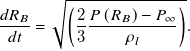(2.9) \begin{align} \frac{dR_{B}}{dt}=\sqrt{\left( \frac{2}{3} \frac{P\left(R_{B}\right)-P_{\infty } }{\rho _{l}}\right)}. \end{align}

Initially, we starts with the bubble nucleus of radius R _B and density per unit volume of liquid n _o . The relationship between the vapour volume fractions to the number of bubble nuclei for a unit volume of mixture fluid is shown in equation (2.10)

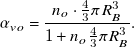(2.10) \begin{align} \alpha _{vo}=\frac{n_{o}\cdot \frac{4}{3}\pi R_{B}^{3}}{1+n_{o}\frac{4}{3}\pi R_{B}^{3}}. \end{align}

The relationship between bubble radius, volume fraction of phase and bubble number density is expressed in equation (2.11)

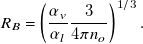(2.11) \begin{align} R_{B}=\left(\frac{\alpha _{v}}{\alpha _{l}}\frac{3}{4\pi n_{o}}\right)^{1/3}. \end{align}

Schnerr and Sauer (Schnerr and Sauer, 2001) proposed the modified mass transfer model by considering equations (2.6–2.11). The modified mass transfer model is defined as in equation (2.12)

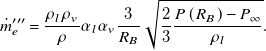(2.12) \begin{align} \dot{m}_{e}^{\prime\prime\prime}= \frac{\rho _{l}\rho _{v}}{\rho }\alpha _{l}\alpha _{v}\frac{3}{R_{B}}\sqrt{\frac{2}{3} \frac{P\left(R_{B}\right)-P_{\infty }}{\rho _{l}}}. \end{align}

Now, n _o and R _B are input parameters for the modified mass transfer model and the standard values are 10⁸ and 10^-5 m, respectively. Thereafter, the next section presents the Lagrangian tracking of a bubble in the cavitation zone.

2.4. Lagrangian tracking of bubbles

In Discrete Phase Model (DPM) in Fluent also termed as Discrete Bubble Model (DBM), Lagrangian approach is used to track the discrete phase (cavity bubbles) in fluid domain, whereas the continuous phase (water) is solved using the transport equation for mass, momentum, and turbulent models. The discrete phase is considered as a point. Each point has its own position, velocity, radius, bubble pressure, etc. Considering these properties bubble-bubble interaction models (coalescence, breakage), bubble–wall interactions and gas diffusion at the bubble interface can be modelled. As the objective of the present research is to observe the phenomenon of CWJM, one-way coupling is used. One-way coupling is applied for interactions between the phases (continuous and discrete). Thus, the mass and momentum equations for the continuous phase are solved in single-phase form, with the resulting velocity and pressure of the continuous phase used to determine the trajectory of the discrete phase by applying additional forces. The mathematical formulation of the models are discussed in details in the authors’ previous publication (Kumar et al., 2024).

2.5. Bubble diameters and statistics

The Lagrangian tracking of cavity bubbles in cavitating flow offers the advantage of individually tracking each bubble, allowing for more precise applications for bubble dynamics. The vapour bubbles of random diameters are injected from the inlet surface. The vapour bubbles are initialised with the fluid velocity in Eulerian reference. Both the phases are in physical, chemical and thermal equilibrium with activated breakage and coalescence models. There are many experimental methods to measure the size of bubbles in the flow domain such as the light transmission method, Mastersizer (Couto et al., 2009), focused beam reflectance measurement (Kail et al., 2009) and acoustic-based spectrometry (Wu and Chahine, 2010). But, it was concluded experimentally, due to low conductance of the gas phases, noise and the interfering signal emitted from the bubbles, these methods failed to predict accurate results.

Therefore, the Sauter mean diameter (SMD) calculates the average bubble size in the flow domain (Kowalczuk and Drzymala, 2016). This parameter, introduced by Sauter in 1926 in his study of fuel oil droplets, is referred as surface–volume mean. The calculation of SMD of different sizes of bubbles considering both volume and surface area of the bubbles is presented in equation (2.13)

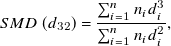(2.13) \begin{align} SMD\left(d_{32}\right)= \frac{\sum _{i=1}^{n}n_{i}d_{i}^{3}}{\sum _{i=1}^{n}n_{i}d_{i}^{2}}, \end{align}

where n _i and d _i are the number and diameter of the individual cavity bubbles, respectively. Currently, SMD is widely recognised for determining the average size of gas bubbles and liquid droplets.

2.6. Impact energy modelling

The surface damage caused by hydrodynamic cavitation on materials primarily occurs in the form of micro-pits, resulting from micro-plastic deformation due to the impact of microjets. Franc (Franc, 2009) performed a phenomenological study of the cavitation erosion process on a ductile material, they shed light on two characteristics scales such as the “time scale” which is the time required for impacts to completely cover the specimen surface and the “length Scale”, this is the critical length for a specimen that governs the erosion behaviour. They also proposed that the incubation time is proportional to the covering time and influenced by the aggressiveness of the flow. The erosion rate under steady-state conditions is determined by the ratio of the hardened layer thickness to the covering time. In the incubation period, the impact pressure resulting from the collapse of a cavitation bubble is complex in both spatial and temporal dimensions, exhibiting unsteady characteristics such as the formation of microjets and shock waves (Brennen, 1995). Hence, a more effective approach for the inverse finite element method (FEM) would be to utilise the impact load generated by the collapse of cavity bubbles. However, for this FEM a Fluid-Structure Interaction (FSI) method must be considered and the authors in Hsiao et al. (2014) and Roy et al. (2015) have pointed out the limitations of such simulations. The only possible way is to use a representative pressure field and analyse how the materials respond to the impact load.

Therefore, an analytical procedure is considered where the shape of the pit is in round shape like a bowl, as shown in Figure 3. The assumed size of the pit from implosion of a cavity bubble is completely characterised by its depth (h _p ) and diameter (d _p ). It is common to assume a pit to be spherical in shape, if the mean aspect ratio of its diameter to depth is large (2012a, Carnelli et al., 2012b; Tzanakis et al., 2014). The assessment of pits can be carried out by analysing the geometrical shape of the deformed part and the plastic strain induced in the region. An analogy is developed between the material deformation caused by microjet liquid impact and spherical indentation. Considering the scope of the current study, the fundamental equations of the spherical indentation tests are considered.

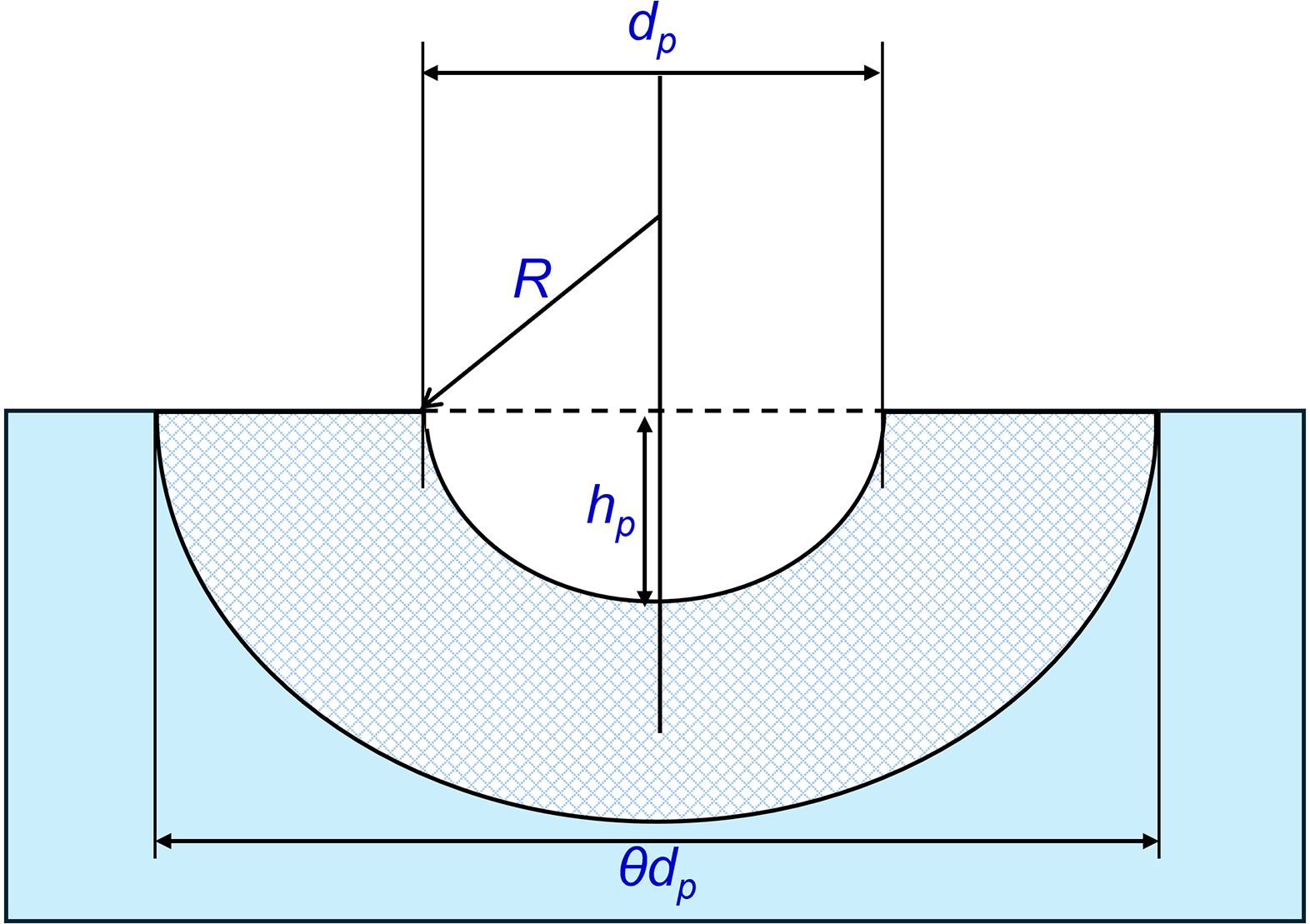
Figure 3. Schematic representation of the spherical geometry used to model cavitation pit, including the extension of the plastically deformed area behind the pit.

Initially, Tabor (Tabor, 1956) has presented the indentation response on the metallic workpiece. Using the definition of true indentation stress (σ) on a metal workpiece, equation (2.14) can be written as

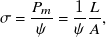(2.14) \begin{align} \sigma = \frac{P_{m}}{\psi }= \frac{1}{\psi }\frac{L}{A}, \end{align}

where P _m and L are the mean contact pressure and indentation load on metal workpiece, respectively, over the projected area A and ψ is a constraint parameter introduced by Francis (Francis, 1976). It was noted that ψ depends on the indentation regime occurring in the core beneath the indenter as expressed in equation (2.15)

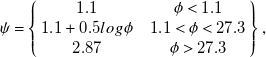(2.15) \begin{align} \psi =\left\{\begin{array}{c@{\quad}c} 1.1 & \phi \lt 1.1\\ 1.1+0.5log\phi & 1.1\lt \phi \lt 27.3\\ 2.87 & \phi \gt 27.3 \end{array}\right\}, \end{align}

where $ \phi $ is a dimensionless parameter associated with the elastic strain at the onset of deformation in the metallic workpiece. If the workpiece is in a purely elastic regime, the constraint factor is 1.1. As the workpiece transitions to an elastic-plastic regime, the constraint factor increases, reaching a maximum value of 2.87 when the regime becomes fully plastic. The representative plastic strain ε and the indentation parameters as proposed by Tabor (Tabor, 1956), are presented in equation (2.16)

(2.16) \begin{align} \epsilon =0.2\frac{d}{D}, \end{align}

where $ \epsilon $ represents the uniaxial strain at the contact edge of the indenter, and d is the diameter of the spherical cap impression created by the spherical indenter having diameter D. The nonlinear relationship between stress and strain, as well as the work hardening occurring on the surface of the workpiece, is modelled using Hollomon’s power law and is represented in equation (2.17)

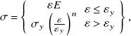(2.17) \begin{align} \sigma =\left\{\begin{array}{cc} \begin{array}{c} \varepsilon E\\ \sigma _{y}\left( \frac{\varepsilon}{\varepsilon _{y}}\right)^{n} \end{array} & \begin{array}{c} \varepsilon \leq \varepsilon _{y}\\ \varepsilon \gt \varepsilon _{y} \end{array} \end{array}\right\}, \end{align}

where σ _y represents the yield stress at reference stress at 0.002 of plastic strain for the specific workpiece material, ε represents the total strain (elastic and plastic), ε _y is the strain at yield point. In the present work the strain value is taken as 0.002, and n is the strain hardening exponent that describes the hardening behaviour of the workpiece sample, which depends on the materials of the workpiece (Bonnavand et al., 2001).

The above fundamental relationship is used to establish the relationship of the pit stress analysis from the microjet impact during implosion of the cavitation bubbles. Therefore, a reverse engineering approach is used to establish the relation between the material deformation with the impact of the microjet and indentation (Carnelli et al., 2012a). The deformation of materials due to the impingement on implosion of an individual sphere-shaped cavity bubble at the surface of the workpiece is known as the cavitation pit. Assuming that a cavitation pit could be like a bowl geometry, and completely described by its depth (h _p ) and diameter (d _p ) for modelling the hydrodynamic impact on the workpiece. The magnitude of pit depth and diameters are used to determine strain at the boundary of the cavitation pit. Considering equation (2.16), the equivalent uniaxial strain ε _p at the contact boundary of the spherical cup-like pit can be expressed as in equation (2.18)

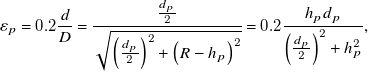(2.18) \begin{align} \varepsilon _{p}=0.2\frac{d}{D}= \frac{\frac{d_{p}}{2}}{\sqrt{\left(\frac{d_{p}}{2}\right)^{2}+\left(R-h_{p}\right)^{2}}}=0.2\frac{h_{p}d_{p}}{\left(\frac{d_{p}}{2}\right)^{2}+h_{p}^{2}}, \end{align}

where d _p and h _p represent the deformed pit diameter and its depth, respectively, with a cavity bubble of radius R. The induced stressσ _p within the cavitation pit can be determined from the stress–strain relationship outlined in equation (2.17), in conjunction with equation (2.18). Therefore, σ _p is expressed in equation (2.19)

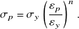(2.19) \begin{align} \sigma _{p}=\sigma _{y}\left(\frac{\varepsilon _{p}}{\varepsilon _{y}}\right)^{n}. \end{align}

After determining the stress induced on the cavitation pit due to the impact of the microjet on the surface of the workpiece, the impact load L _p as in equation (2.20) can be derived from the relationship shown in equation (2.14)

(2.20) \begin{align} L_{p}=\sigma _{p}\psi A_{p}. \end{align}

After calculating the impact load, the final step is to determine the hydrodynamic impact pressure (σ _H ) produced during the implosion of the cavity bubble. This is derived by considering the geometrical characteristics of the needle-like pits and the induced stress. For calculation of hydrodynamic impact stress (σ _H ), it is assumed that the load L _p measured from the pit stress is equivalent to the hydrodynamic load L _H released during the implosion of the cavity bubble. It is basically the impact load generated on surface of the workpiece due to the microjet and the expression is shown in equation (2.21)

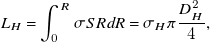(2.21) \begin{align} L_{H}=\int _{0}^{R}\mathit{\sigma }SRdR=\sigma _{H}\pi \frac{D_{H}^{2}}{4}, \end{align}

where S represents the perimeter of the impacted area and D _H is the effective hydrodynamic distance, defined as the diameter of the microjet in this study. The diameter of the microjet is equal to 1/10th of the resonant bubble diameter, as explained in previous studies (Tezel and Mitragotri, 2003). Furthermore, the theory of bubble collapse proposed by Rayleigh (Rayleigh, 1917) is considered where the maximum energy (E _b ) released due to implosion of the cavity bubble is expressed as in equation (2.22)

(2.22) \begin{align} E_{b}=\frac{4}{3}\pi \left(P_{\textit{static}}-P_{\textit{vapour}}\right)R_{\textit{resonant}}^{3}, \end{align}

where P _static and P _vapour represent the static pressure and vapour pressure inside the bubble (3500 Pa at 27 °C), respectively, and R _resonant is the resonant radius of the bubble. The energy equation states that the energy of a cavity bubble is determined by its maximum volume and the associated pressure gradient. The energy generated by the bubble is then transformed into significant kinetic energy, propelling the microjet toward the surface of the workpiece. The hydrodynamic impact of microjet causes a high pressure and its magnitude can be obtained from the water hammer of equation (2.23) (Tijsseling and Anderson, 2004)

(2.23) \begin{align} \sigma _{H}=\rho _{l}C_{l}\left(\frac{\rho _{s}C_{s}}{\rho _{l}C_{l}+\rho _{s}C_{s}}\right)V_{jet}, \end{align}

where ρ _l and C _l represent the density and speed of sound in the liquid medium. Similarly, ρ _s and C _s are the relating parameters for the workpiece.

2.7. Numerical simulation set-up

The model was implemented within the commercial CFD software package ANSYS Fluent, version 18.1. The complete simulation process is illustrated in Figure 4, which begins with the creation of a geometric model, followed by mesh generation and boundary definition. Subsequently, the solution convergence is verified, and upon achieving convergence, the results are visualised. This is followed by selection of the output parameters for the grid independence test to ensure the desired accuracy while minimising computation time.

Figure 4. Multiphase CFD simulation approach.

The numerical method for simulating cavitation phenomenon in the flow domain starts with initialising the solution using specific boundary conditions and fluid properties. This is followed by solving the RANS equation, turbulence model and cavitation model. The mass transfer equation is solved to capture the interaction between the bulk liquid and discrete phases. Once convergence criteria are met, these equations are iteratively solved for the n time step.

3. Results and discussion

The CFD simulations are conducted using the above stated governing equations and turbulence model. The selected flow domain and initial boundary conditions for the simulation are detailed in subsequent sections.

3.1. Numerical simulation

The Eulerian mixture model is selected to simulate the multiphase scenario, excluding both the slip velocity between the phases and the influence of the gravitational force. In addition, heat transfer is assumed to occur under isothermal conditions. The turbulence is modelled using the realisable k − ε model including a standard wall function. Cavitation phenomenon are modelled using the Schnerr-Sauer model (Schnerr and Sauer, 2001) with the bubble number density as 10⁸, accounting for the effect of turbulence on cavitation phenomenon. The Semi-Implicit Method for Pressure Linked Equations (SIMPLE) scheme is selected for the solution method, as it couples pressure and velocity. Additionally, PRESTO! is chosen for the pressure calculation. Spatial discretisation is implemented using the least square cell-based approach for the momentum equation employing a second-order upwind scheme. Conversely, for the turbulence model first-order upwind scheme is chosen.

3.1.1. Flow geometry and boundary conditions

In present study, the orifice which has l/d>0.5 is selected for modelling. The flow direction and mesh element for further analysis are shown in Figure 5(a) and (b), respectively. A quadrilateral mesh is used to discretise the flow domain, with size functions based on proximity and curvature. Successively, the fourteen equally spaced planes are created downstream of the flow domain, each separated by a 10 mm gap, as illustrated in Figure 6. These planes are key locations for observing significant flow properties within the flow domain. They will play a crucial role in identifying the cavitation zone during CWJM and CWJP.

Figure 5. Three-dimensional (3-D) flow domain with meshing. (a) Computational fluid domain. (b) Quadrilateral mesh element for computational analysis.

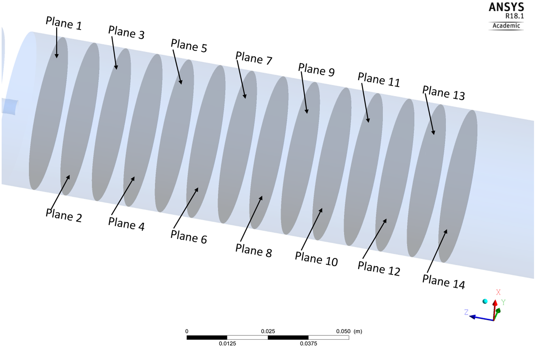
Figure 6. Created planes to delineate cavitation zone on downstream side of the computational flow domain.

The isometric view of the sampling planes is shown where computational results from CFD analysis are collated for identification of the cavitation zone.

In the present CFD computation, liquid and vapour are selected as the primary and secondary phases, respectively. The density and viscosity of the primary phase are 998.2 kg m⁻³ and 0.001002 kg/m-s, respectively, whereas the density and viscosity of the secondary phase are 0.02558 kg m⁻³ and 1.26 × 10⁻⁶ kg/m-s, respectively. The initial boundary conditions at the inlet are set as 1 m s⁻¹, similarly 0.1 MPa is set at the outlet boundary, and the saturated vapour pressure is set at normal room temperature i.e. 0.00354 MPa.

The behaviour of the fluid flow is observed through a single hole orifice plate of thickness 10 mm that is installed in the middle of the pipe, which has a length of 0.4 m. Hence, the realistic parameters for the governing equations are taken for simulating the pressure, velocity, vapour volume fraction and phase interactions during the flow.

3.1.2. Grid independence test

The mesh independence analysis is performed with the CFD model, and the results are presented in Figure 7. In this analysis, the velocity at the inlet is set to 0.3 m s⁻¹ and the outlet pressure is kept at 0.1 MPa. The velocity of the fluid at the entrance of the orifice is selected as the output parameter. It is observed that the velocity at the orifice entrance increases rapidly as the number of mesh elements increases. The maximum output (velocity) is attained with a fine mesh is applied at the orifice, using a grid count of approximately 100,000 elements. Therefore, a finer mesh is selected at the orifice region because of the significant velocity difference and narrowing in the flow area. The velocity curve demonstrates grid independence, indicating that additional refinement or an increase in the grid count would have a minimal impact on the response. Through this approach, computational resource is optimised while ensuring desired accuracy in the computation results. For the current work 100,000 mesh elements are selected.

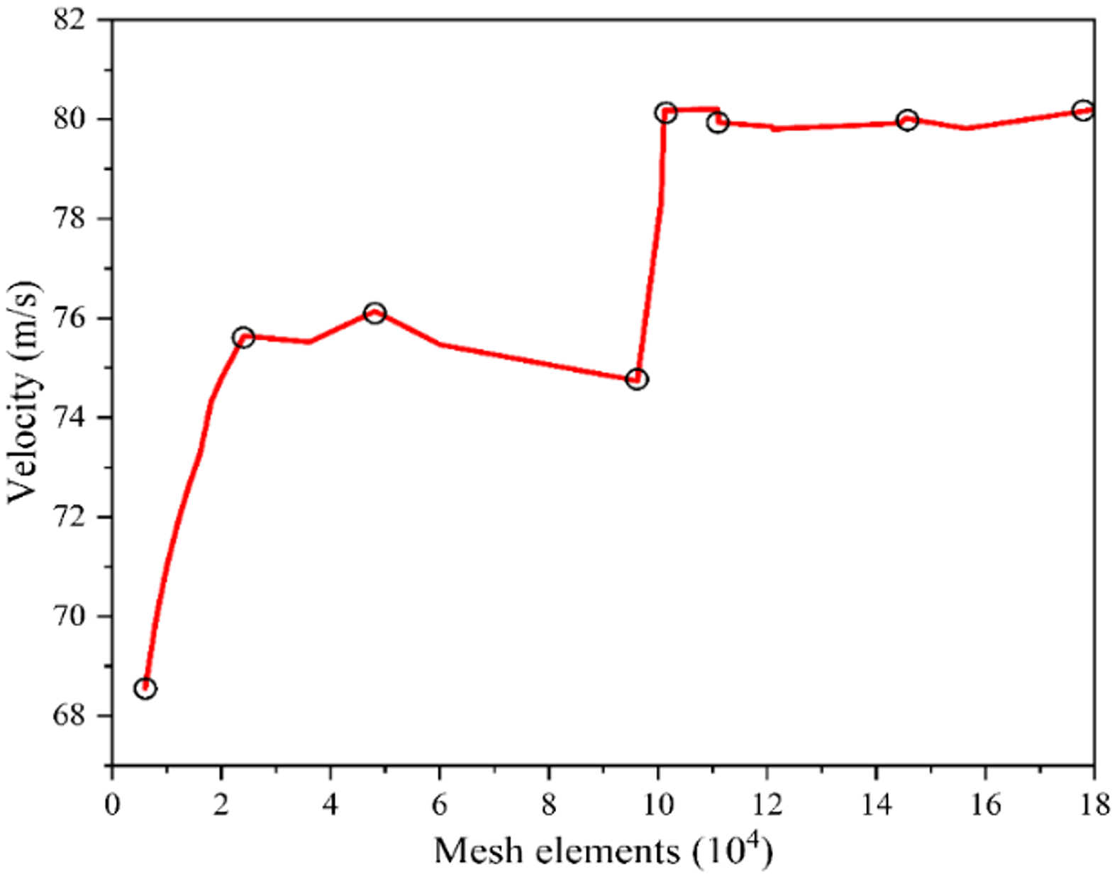
Figure 7. Grid analysis assessment.

3.1.3. Model validation

To validate the chosen computation scheme, different inlet velocities of fluid are input into the same flow geometry and the numerical results are simulated. The static pressure and CN with different flow velocity are depicted in Figure 8, and it can be seen that the increase in flow velocity in the flow domain led to linear increase in the static pressure, and further validated with Bernoulli’s equation and CN in equation (2.1).

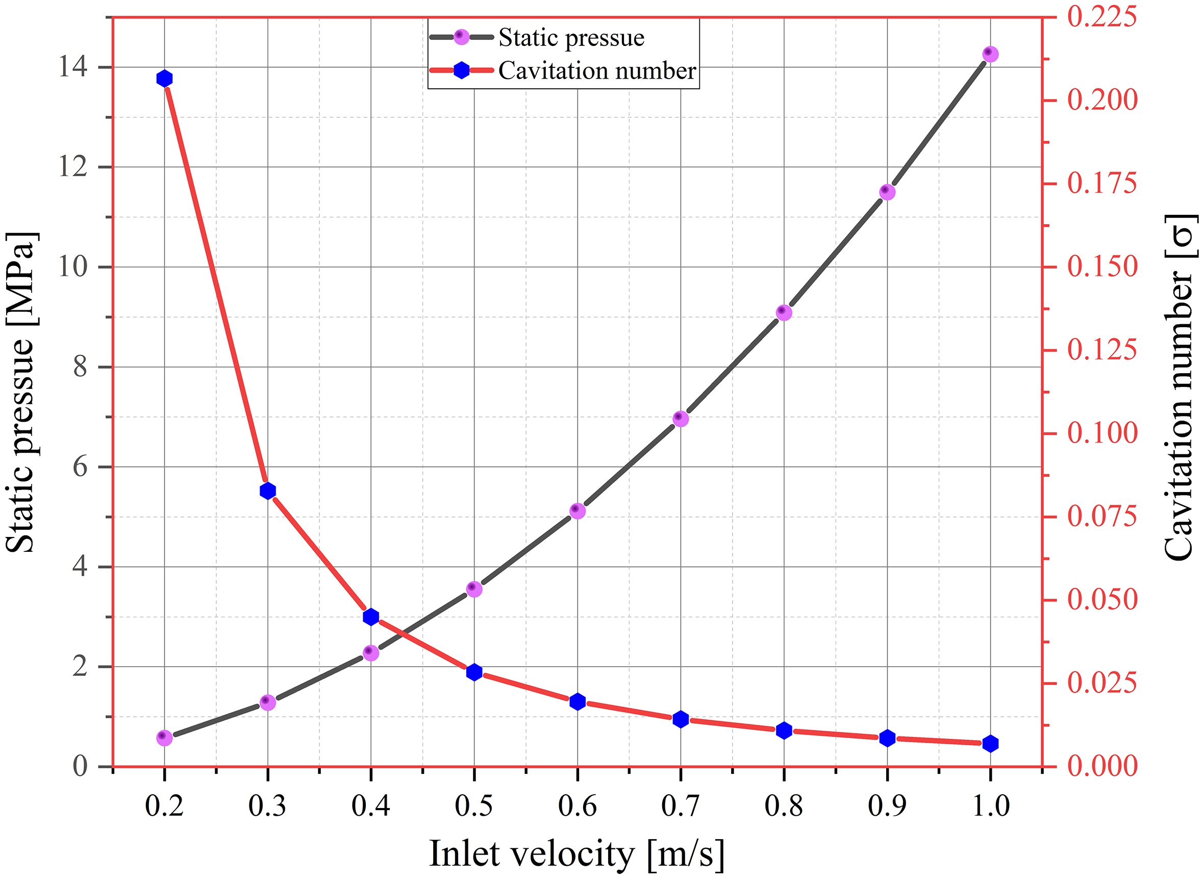
Figure 8. Static pressure and its corresponding the CN at different inlet velocities.

Figure 9 is another validation graph with dimensionless parameters i.e. the Reynolds number presented in equation (3.1) below, with the waterjet velocity coming out from the orifice with respect to a different velocity inlet

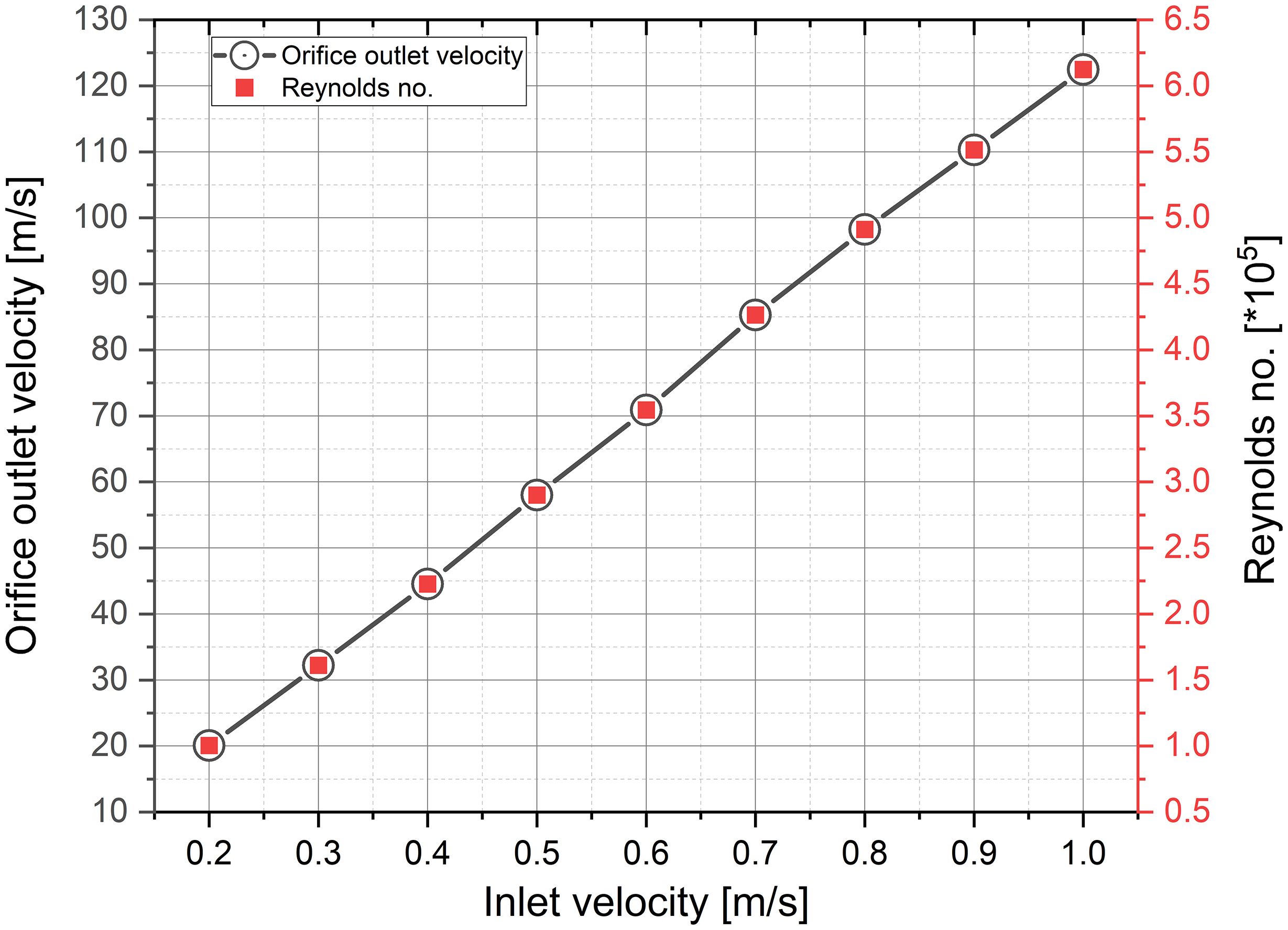
Figure 9. Waterjet velocity and corresponding Reynolds number atdifferent inlet velocities.

(3.1) \begin{align} Re=\frac{\rho _{l}vd_{o}}{\mu }. \end{align}

It can be concluded that high static pressure and low CN confirm the formation of cavitation bubbles whereas, high velocity and high Reynolds number led to the formation of a high-speed cavitating waterjet. The cavitating waterjet is identified by performing a detailed analysis of the parameters such as CN, drop in pressure, flow velocity, fraction of vapour and phase interaction. In this study, the CN is set to 0.007. A lower CN is chosen to expedite the cavitation phenomenon.

3.2. Determination of standoff distance for machining and peening

The CN is just one of the parameters to map the initiation of cavitation phenomenon in a fluid domain. Therefore, additional parameters like pressure drop, jet velocity and vapour volume fraction are employed to address the present objectives, as discussed in the following sections.

3.2.1. Pressure distribution in the flow domain

The initiation of cavity bubbles occurs when the static pressure drops to or below the vapour pressure at the working temperature of the carrier fluid. The bubbles continue to grow in the low-pressure zone and collapse upon reaching the high-pressure region. Therefore, computation of the static pressure is necessary to identify the cavitation zone in the flow domain. The computation of the static pressure contour on created planes on the downstream side is shown in Figure 10. From the contour legend, it can be observed that the low-pressure region is maintained from 0.225 to 0.295 m downstream, as indicated by sampling planes 3 to 8. Subsequently the high-pressure region is observed from sampling plane 9 onwards in the flow domain.

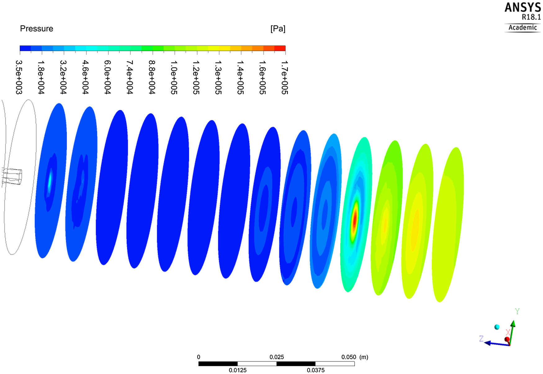
Figure 10. Pressure contour at created planes within the fluid domain.

Therefore, from Figure 10, it can be concluded that the low-pressure region is maintained up to 70 mm in the axial direction of the flow domain. This implies that the workpiece should be placed up to maximum distance of 70 mm from the orifice on the downstream side for an effective CWJM.

3.2.2. Jet velocity

The velocity of a cavitating waterjet coming from the orifice is also one of the important parameters. Computational results from the CFD are analysed to identify the accurate standoff distance to place the workpiece for CWJM. The velocity contour plot is shown in Figure 11, and it can be observed that the high velocity cavitating waterjet is available up to the second sampling plane from the opening of the orifice. This implies that a high velocity of the cavitating jet is maintained up to 20 mm distance on downstream side. Therefore, placing the workpiece at 20 mm from the opening of the orifice will result in CWJM, in contrast, placing the workpiece between 20 and 70 mm will lead to the CWJP effect on the active surface of the workpiece.

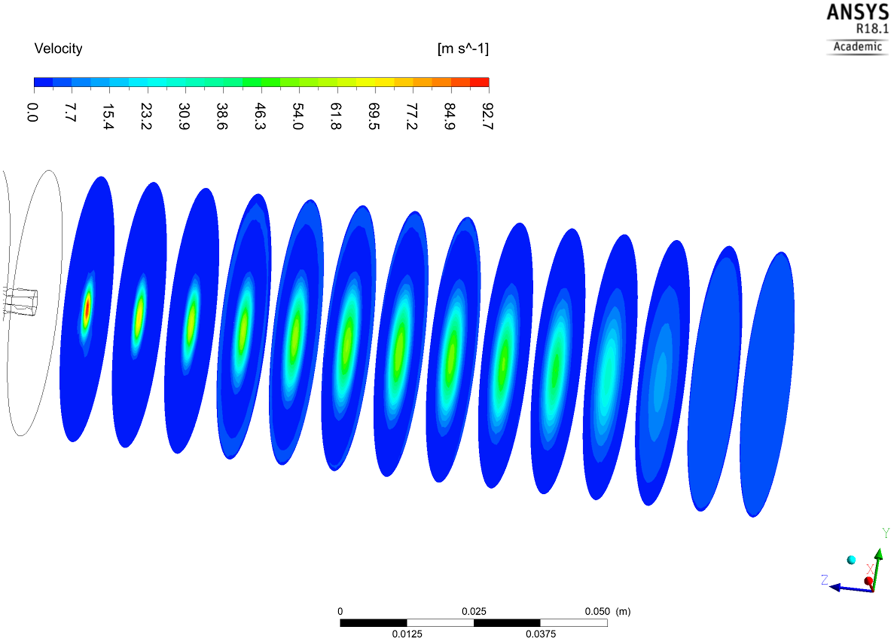
Figure 11. Velocity contour plot at various created planes within flow domain.

3.2.3. Effect of volume fraction

The volume fraction in a flow domain is stated to the space occupied by each phase in a unit volume. This parameter is computed to assess the intensity of the cavitation phenomenon, as the extent of cavitation inception is linked to the value representing the vapour phase. A high vapour fraction indicates a significant mass transfer rate from the liquid to the vapour phase, resulting from the low static pressure in the flow domain. The high volume fraction of vapour intensifies the cavitation activity in a fluid domain (Guide, 2013). Initially, the volume fraction of the mixture (liquid and vapour) is set to 1 to solve equation (2.6), ensuring that the solutions for both phases remain complementary. Therefore, the contour of vapour volume in the computational domain is analysed on the various sampling planes and the results are shown in Figure 12. The computational analysis of this parameters helps in determining the optimum standoff distance for the cavitation peening effect in the cavitation chamber.

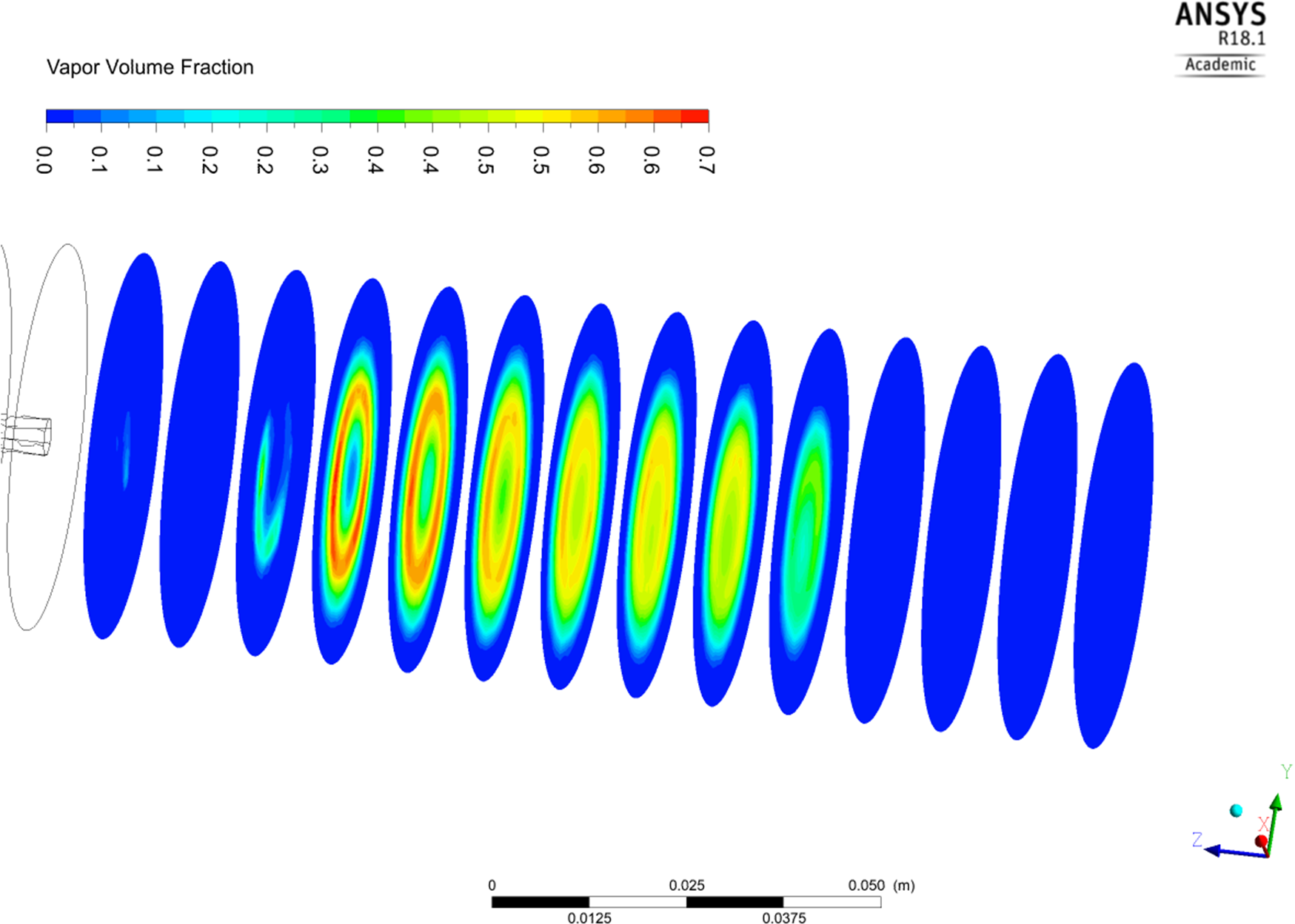
Figure 12. Contour plot of volume fraction (vapour) on created planes within flow domain.

From Figure 12, the maximum value of vapour fraction is 0.7, which lies from sampling plane 4 to sampling plane 10, and the occurrence of cavity bubbles in this region is very high. Thus, the workpiece should stay in this zone, which will yield a greater probability of getting the peening effect on the active layer of the workpiece surface due to the implosion of cavity bubbles. For CWJM, the volume fraction of vapour (α _v ) must exceed 0.6. As a result, the legends of the contour plane help to identify the region with a high concentration of bubble clouds within the flow domain, extending from 245 to 305 mm from the orifice exit. In addition, it can be observed that the high volume of vapour is visible up to 60 mm in the longitudinal direction i.e. Z-axis, with the chosen geometry of the orifice plate. It is also evident from the figure that the 4th sampling plane has a vapour fraction with a shape of a ring, hence there is a need to analyse this parameter further on the remaining planes of the fluid domain. This analysis will be helpful for the precise identification of the cavity bubble cloud in the flow domain to observe both the cavitation phenomenon and CWJM.

The contours of the volume fraction of vapour in planes 3 to 12 are presented in Figure 13. It is evident that the volume fraction of vapour decreases from plane 4 and reaches zero in plane 12. This result indicates other planes on the downstream side are not important for mapping the bubble cloud. In addition, Figures 12 and 13 show that the bubble cloud is observable from 245 to 305 mm in the longitudinal direction of the flow domain. Consequently, if a workpiece is positioned in this region, there is a high likelihood that the collapse of cavity bubbles could damage the workpiece.

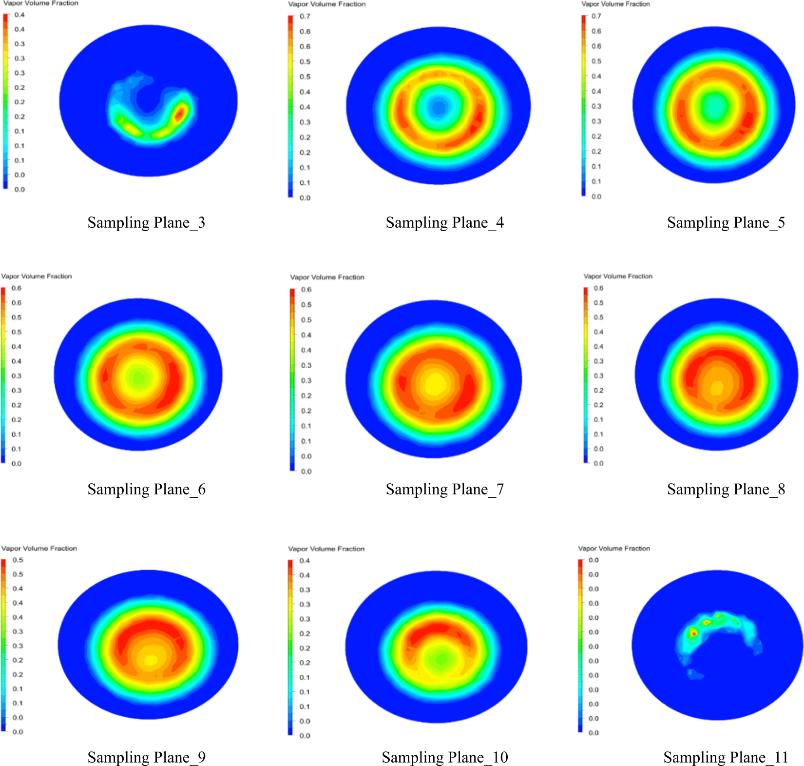
Figure 13. Contour plot of volume fraction (vapour) on specific sampling planes within domain.

3.3. Bubble characteristics for machining and peening

The objective is to comprehend the dimension and bubble number statistics that cause the workpiece to erode. The detailed mathematics for Lagrangian tracking of bubbles is discussed in Section 2.4. The computation of bubble statistics and its SMD on various planes is discussed in section 2.5. Lagrangian tracking demands significant computational resources and time. When the sampling planes are spaced 10 mm apart, the computational load becomes excessive and time consuming. Therefore, the sampling planes are positioned 25 mm apart within the flow domain to optimise performance, as in Kumar et al. (2024).

The bubble distribution at the selected sampling planes is displayed in Figure 14. The number of cavity bubbles and the SMD are represented on the left and right sides of the Y-axis, respectively, while the axial position of each sampling plane is indicated on the X-axis. From Figure 14, it can be noted that the breaking phenomenon of the cavity bubble from the continuous phase is constant up to 45 mm (plane at 250 mm) from the exit of the orifice at 205 mm. This observation suggests that the workpiece should be positioned before this point, where the waterjet and cavity bubbles exert a synergistic effect. The perfect coalesce and accumulation of cavity bubbles can also be observed at 70 mm, from sampling the plane at 275 mm to the opening of the orifice. Therefore, the workpiece must be placed within 20 mm distance from the opening of the orifice where the erosion of materials will have high chance due to the combined effect of the waterjet and cavitation phenomenon. Similarly, placement of the workpiece at a distance of 70 mm from the orifice will have a high chance of the peening effect on the active surface of the workpiece. These computational results are in good alignment with the results available in the literature, which are validated with the experimental results obtained by Soyama et al. (Soyama et al., 2001).

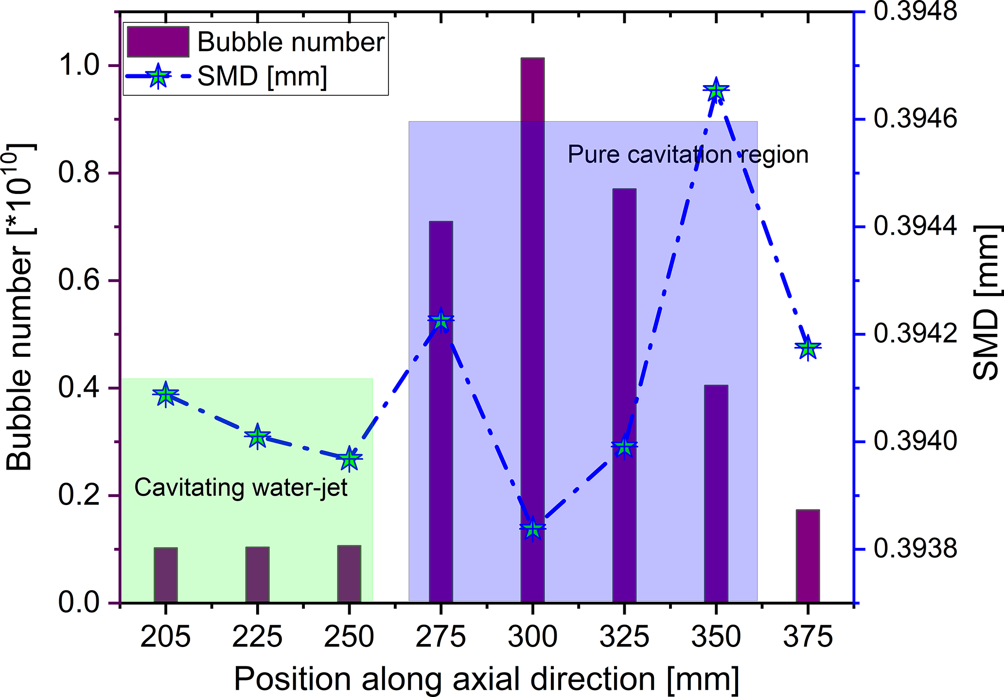
Figure 14. Bubble statistic and SMD on planes in the fluid domain.

3.4. Calculation of impact energy for machining and peening

The calculation of impact pressure and hydrodynamic effects on the workpiece resulting from the collapse of a cavity bubble has been discussed in section 2.6. Tzanakis et al. (Tzanakis et al., 2014) carried out experimental studies using a high-speed camera to estimate the geometric features of the bubble and microjet. Considering the scope of the present study, the geometry of a cavity bubble is assumed as spherical and its average diameter is taken as 390 µm in the cavitation chamber away from the surface of the workpiece, as obtained from the simulation study presented in Figure 14. The obtained geometrical parameters are then used to calculate the pressure and hydrodynamic impact on workpieces of different materials.

Considering the analogy from the indentation test carried out by Tzanakis et al. (Tzanakis et al., 2014). The diameter of the microjet, which is nothing but the hydrodynamic impact diameter, enhances the accuracy of pressure estimation on the workpiece. From the experimental study of Tzanakis et al. (Tzanakis et al., 2014) on various individual spherical bubbles near to a surface boundary of the workpiece just before the implosion of the cavity bubble, it was found that their average resonant diameter was 100 µm, which is 1/4th of the cavity bubble diameter in the present simulation. This is also in the agreement with the study carried by Tzanakis et al. (2011, 2014). The experimental study carried out by Tesel and Mitragotri (Tezel and Mitragotri, 2003) for the effective hydrodynamic diameter of the microjet is approximately 1/10th of the maximum radius of the cavity bubble when these are near the active surface of the workpiece. Therefore, the effective jet diameter of the microjet is chosen as equal to 1/10th of the resonant bubble diameter when it is near to the active surface of the workpiece, which is in good agreement with the studies conducted by Tzanakis et al. (2011).

Therefore, the computation of hydrodynamic impact is carried out considering the dimension of the pit area obtained in Tzanakis et al. (2014) through experimental investigation. The average pit diameter ranged from 6 to 7 µm, while the average pit depth ranged from 0.13 to 0.15 µm. The bubble energy in the present study, calculated using the relation provided in equation (2.22), is found to be 5.12 × 10⁻⁸ J for the hydrodynamic cavity bubble.

The computational analysis is based on the plastic strain regime of a pit and its geometrical dimensions. As a result, the hydrodynamic impact pressure and the velocity of the microjet affecting the surface of the selected material from the implosion of a single hydrodynamic cavitation bubbles are discussed below.

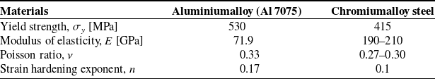
The sample material used in this study is chromium steel (AISI 50100) and aluminium alloy (7075 T651) to identify the hydrodynamic loads from the implosion of the cavity bubble. The mechanical properties of the selected sample are presented in Table 1.

Table 1. Tested materials and main properties

The hydrodynamic pressure of the microjet impacted on the sample surface is obtained from equation (2.20) and presented in Figure 15. From the experimental investigation Tzanakis et al. (Tzanakis et al., 2014) had chosen six deformed pit areas randomly and the results are presented on the x-axis of the figure. The area of deformed pits is calculated using the equation (3.2)

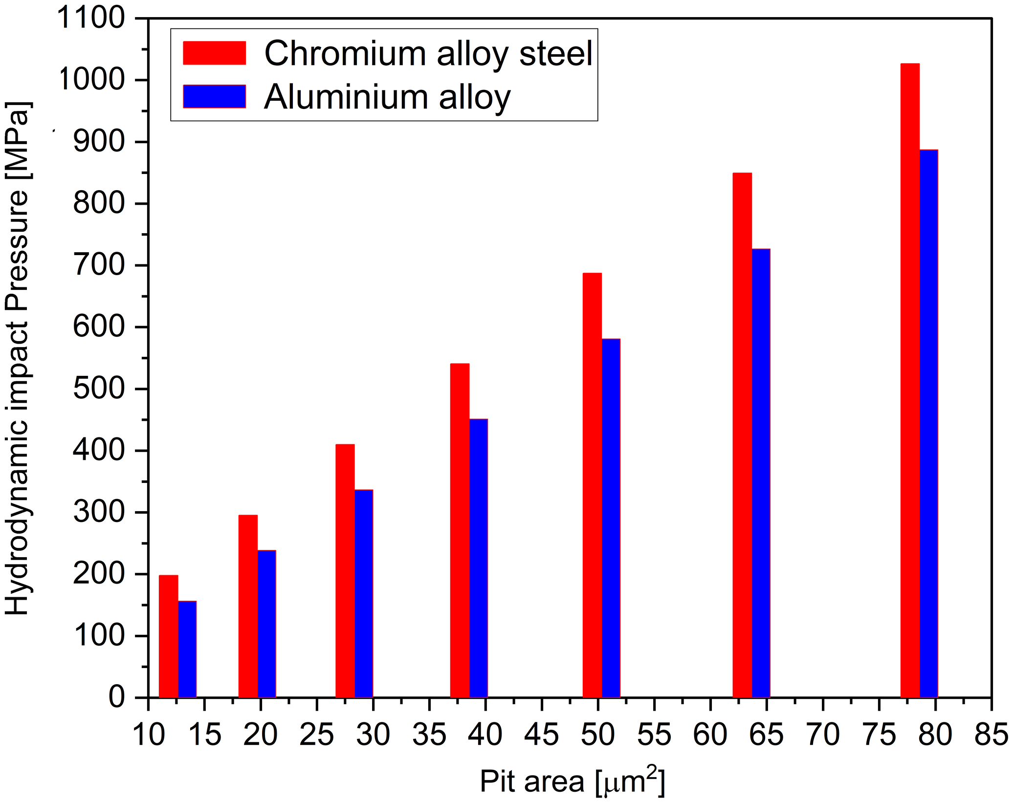
Figure 15. Impact pressure on implosion of a cavity bubble as a function of eroded pit area.

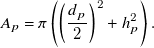(3.2) \begin{align} A_{p}=\pi \left(\left(\frac{d_{p}}{2}\right)^{2}+h_{p}^{2}\right). \end{align}

Figure 15 shows that the area of deformation on both samples is linearly proportional to the hydrodynamic impact pressure generated on collapse of a cavity bubble. This outcome indicates a strong relationship with the deformed pit size and the impact pressure. Additionally, the deformation of the pit is heavily influenced by the length of the hypotenuse of the orthographic projection, which is determined by the diameter and depth of the pit relative to the centre of the spherical cup.

It can also be observed that the aluminium alloy needs a higher impact pressure than the chromium alloy steel sample, this is because the yield strength of aluminium alloy is equivalent to 530 MPa, whereas the yield strength of the chromium alloy sample is equivalent to 415 MPa. According to the results the liquid microjet can certainly erode the surface, especially when the collapse point is near to the surface, γ < 1. The present findings are very much aligned in the same direction as the previous investigation that concluded that microjets contribute to the actual damage of the materials if the impact pressure is higher than the yield strength of the materials (Tomita and Shima, 1986).

The results indicate that pit formation can still occur even when the impact pressure is lower than the yield strength. This is because of plastic deformation and depression patterns developed in regions with softer areas within the material (local yielding). This is mainly dependent on the crystal structure of the materials. Similarly, in the present study, the pit formation on the sample material’s surface can occur at a hydrodynamic impact pressure of 205 MPa and 160 MPa in the aluminium alloy sample and chromium alloy steel, respectively.

The velocity of the microjet is responsible for creating the erosion and surface modification in the specified samples. The velocity of the microjet is obtained by the water hammer equation presented as in equation (2.23). In addition, the hydrodynamic impact pressure has a linear relationship with the velocity of the liquid microjet, as shown in Figure 16 (right), although the occurrence of very intense events results in larger pit size and plastic deformation. This can be associated with the extreme microjet velocity of up to 800 m s⁻¹ and a weak impact can also occur when the microjet velocity is less than 200 m s⁻¹.

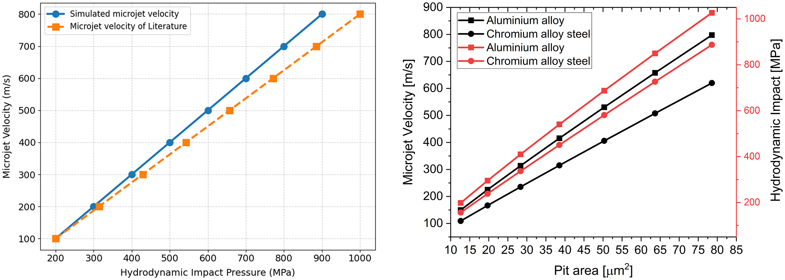
Figure 16. Validation of microjet velocity and hydrodynamic impact of present study (left) and velocity of a microjet on implosion of a cavity bubble as a function of hydrodynamic impact pressure and pit area (right).

The microjet obtained in the present work is in strong agreement with the literature by Grant and Lush (Grant and Lush, 1987) as shown in Figure 16 (left) and Wood et al. (Wood et al., 1967). They recorded the velocity of a microjet during the implosion of a hydrodynamic cavity bubble, which lies in the range of 100 to 500 m s⁻¹, considering the results of the present finding and the cavitation bubble dynamics relationship of earlier research by the author (Kumar et al., 2024).

Therefore, conclusions can be drawn, such as the synergistic effect of the cavity bubble can be used for micro-machining, surface modification and the peening of the machined surface to enhance its fatigue life by inducing the compressive residual stress instead of shot peening. However, the material response and parametric analysis are not covered in the present studies. The application of this novel CWJM method will lead to a cleaner as well as a sustainable machining method for industries with zero carbon footprints.

4. Conclusions

A comprehensive simulation study has been performed to predict the location for machining and peening of materials using a cavitating waterjet in a flow domain. The computed standoff distance is 20 mm from the orifice exit for CWJM, while the workpiece is positioned 70 mm downstream from the orifice exit, resulting in cavitation peening. In addition, the aggressiveness of the cavitation phenomenon with a waterjet and without a waterjet will take place up to 40 mm and 70 mm, respectively. Along with the multiphase computational study, the DPM is used to determine bubble statistics and the SMD at different sampling planes in the flow domain for the CWJM. The analytical study based on a reverse engineering approach has also been carried out to predict the magnitude of the hydrodynamic impact pressure generated due to implosion of a cavity bubble. In this work, aluminium alloy (Al 7075) and chromium alloy steel (AISI 50100) are chosen to compute the hydrodynamic impact pressure that will be helpful for erosion prediction.

Computational simulations reveal a linear relationship between hydrodynamic pressure and microjet velocity. The severity of cavitation phenomenon and the magnitude of the hydrodynamic impact pressure are measured by the area of the eroded pit on the specimen. The hydrodynamic impact pressure and jet velocity can be compared with the actual damage patterns on the specimen’s surface, which may vary significantly with the size and geometry of the eroded pits.

The insights gained from this study will assist designers in optimising applications and determining the appropriate standoff distance for material processing, whether for material removal or surface modification. It also provides design guidelines of a cavitation chamber for CWJM. The influence of critical pressure ratio between upstream and downstream side needs to be investigated further and its impact on cavitation zone needs to be explored in future.