Mutation graph of support $\tau $-tilting modules over a skew-gentle algebra

Abstract

Let $\mathcal {D}$ be a Hom-finite, Krull-Schmidt, 2-Calabi-Yau triangulated category with a rigid object R. Let $\Lambda =\operatorname {End}_{\mathcal {D}}R$ be the endomorphism algebra of R. We introduce the notion of mutation of maximal rigid objects in the two-term subcategory $R\ast R[1]$ via exchange triangles, which is shown to be compatible with the mutation of support $\tau $-tilting $\Lambda $-modules. In the case that $\mathcal {D}$ is the cluster category arising from a punctured marked surface, it is shown that the graph of mutations of support $\tau $-tilting $\Lambda $-modules is isomorphic to the graph of flips of certain collections of tagged arcs on the surface, which is moreover proved to be connected. Consequently, the mutation graph of support $\tau $-tilting modules over a skew-gentle algebra is connected. This generalizes one main result in [49].

1 Introduction

Cluster algebras were introduced by Fomin and Zelevinsky [27] around 2000. The geometric aspect of cluster theory was explored and developed by Fomin, Shapiro and Thurston [25] and Labardini-Fragoso [40], where they construct a quiver with potential [23] from any triangulation of a marked surface. However, cluster categories of acyclic quivers were introduced by Buan, Marsh, Reineke, Reiten and Todorov [14] in order to categorify cluster algebras, which were generalized later by Amiot [2] to cluster categories of quivers with potential.

The indecomposable objects in the cluster category from a marked surface without punctures are classified via curves by Brüstle and Zhang [13], where the Auslander-Reiten translation is realized by the rotation. The dimension of $\operatorname {Ext}^1$ between certain indecomposable objects is shown by Zhang, Zhou and Zhu [53] to equal the intersection number between the corresponding curves, and the middle terms between such extensions are explicitly described by Canakci and Schroll [17] via smoothing. The Calabi-Yau reduction introduced by Iyama and Yoshino [35] in this case is interpreted via the cutting of the surface by Marsh and Palu [44]. For the punctured case (with nonempty boundary), Brüstle and Qiu [12] realize the Auslander-Reiten translation via the tagged rotation, Qiu and Zhou [49] classify certain indecomposable objects via tagged curves and show the equality between the dimension of $\operatorname {Ext}^1$ and the intersection number, and Amiot and Plamondon [5] give another approach via group actions and orbifolds.

The Jacobian algebra of the quiver with potential associated to a certain triangulation of a marked surface with nonempty boundary is a skew-gentle algebra with some properties (e.g., Gorenstein dimension at most one) [8, 30, 49]. Skew-gentle algebras were introduced by Geiß and de la Peña [31], whose indecomposable modules are classified by Bondarenko [10], Crawley-Boevey [19] and Deng [22], and whose morphism spaces are described by Geiß [29]. In a previous work [33], we give a geometric model of the module category of an arbitrary skew-gentle algebra, inspired by the geometric model [49] of cluster categories of punctured marked surfaces and the geometric model of the module categories of gentle algebras given by Baur and Simões [9]. There is also some work on geometric models of the derived categories of gentle/skew-gentle algebras; cf., for example, [32, 43, 46, 45, 6, 4, 3, 42].

Adachi, Iyama and Reiten [1] introduced $\tau $ -tilting theory to generalize the cluster structure to arbitrary finite-dimensional algebras via mutation of support $\tau $ -tilting modules. The support $\tau $ -tilting modules have been found to be deeply connected with other contents of representation theory, such as functorially finite torsion classes, 2-term silting objects, cluster tilting objects and immediate t-structures. In contrast to the classical tilting case, where an almost complete tilting module may have exactly one complement, any support $\tau $ -tilting module can always be mutated at an arbitrary indecomposable direct summand to obtain a new support $\tau $ -tilting module. The exchange graph $\operatorname {EG}(\operatorname {s\tau -tilt} A)$ of support $\tau $ -tilting modules of a finite-dimensional algebra A has (isoclasses of) basic support $\tau $ -tilting modules over A as vertices and has mutations as edges. One important problem is to count the number of connected components of $\operatorname {EG}(\operatorname {s\tau -tilt} A)$ .

In our previous work [33], using a geometric model, we classify support $\tau $ -tilting modules of skew-gentle algebras via certain dissections of marked surfaces. In the current paper, after establishing a framework for the theory of mutation in two-term subcategories of a 2-Calabi-Yau triangulated category, we generalize the geometric model from skew-gentle algebras to the endomorphism algebras of rigid objects in the cluster categories arising from punctured marked surfaces. One important application is the connectedness of the exchange graph $\operatorname {EG}(\operatorname {s\tau -tilt} A)$ for A an arbitrary skew-gentle algebra. This generalizes the main result in [28] where A is a gentle algebra, and one main result in [49] where A is a skew-gentle Jacobian algebra.

We also note that it is shown in [7] that $\operatorname {EG}(\operatorname {s\tau -tilt} A)$ has one or two components in the case that A is a complete gentle (or, more generally, special biserial) algebra. See [11, 38, 52] for some related results.

The paper is organized as follows. In Section 2, we introduce and investigate mutation in two-term subcategories of a 2-Calabi-Yau triangulated category. In Section 3, we recall basic notions and results on the cluster categories from punctured marked surfaces. In Section 4, we give a geometric model for the endomorphism algebra of a rigid object in the cluster category arising from a punctured marked surface and show that this includes the class of skew-gentle algebras. Moreover, we classify support $\tau $ -tilting modules via certain dissections. In Section 5, we introduce the notion of flip of dissections and show that it is compatible with the mutation of support $\tau $ -tilting modules. As an application, the connectedness of the exchange graph of support $\tau $ -tilting modules over a skew-gentle algebra is obtained.

Convention

Throughout this paper, we assume ${\mathbf {k}}$ to be an algebraically closed field. Any additive category $\mathcal {D}$ in this paper is assumed to be

1. (1) ${\mathbf {k}}$ -linear and Hom-finite (i.e., $\operatorname {Hom}_{\mathcal {D}}(X,Y)$ is a finite-dimensional vector space over ${\mathbf {k}}$ for any pair of objects $X,Y$ ), and

2. (2) Krull-Schmidt (i.e., any object is isomorphic to a finite direct sum of objects whose endomorphism rings are local).

We use $X\in \mathcal {D}$ to denote that X is an object in $\mathcal {D}$ . For any $X\in \mathcal {D}$ , denote by

1. (1) $|X|$ the number of isomorphism classes of indecomposable direct summands of X,

2. (2) $\operatorname {add} X$ the additive hull of X, that is, the smallest subcategory of $\mathcal {D}$ , which contains X and is closed under isomorphisms, finite direct sums and direct summands, and

3. (3) ${}^\perp X$ and $X^\perp $ the full subcategories of $\mathcal {D}$ consisting of all objects Y such that $\operatorname {Hom}_{\mathcal {D}}(Y,X)=0$ and $\operatorname {Hom}_{\mathcal {D}}(X,Y)=0$ , respectively.

We call $X\in \mathcal {D}$ basic if $|X|$ is the number of indecomposable direct summands of X (i.e., any two distinct indecomposable direct summands of X are not isomorphic). For any object $X\in \mathcal {D}$ and any direct summand Y of X, we denote by $X\setminus Y$ the direct summand of X such that $X=Y\,{\oplus}\, (X\setminus Y)$ .

We call a morphism $g\in \operatorname {Hom}_{\mathcal {D}}(X,Y)$ right minimal if for any $h\in \operatorname {Hom}_{\mathcal {D}}(X,X)$ such that $g\circ h=g$ , we have that h is an isomorphism. For any subcategory $\mathcal {T}$ of $\mathcal {D}$ , we call $f\in \operatorname {Hom}_{\mathcal {D}}(X,Y)$ a right $\mathcal {T}$ -approximation of $Y\in \mathcal {D}$ if $X\in \mathcal {T}$ and

$$\begin{align*}\operatorname{Hom}_{\mathcal{D}}(-,X)\xrightarrow{\operatorname{Hom}_{\mathcal{D}}(-,f)}\operatorname{Hom}_{\mathcal{D}}(-,Y)\longrightarrow0\end{align*}$$

is exact as functors on $\mathcal {T}$ . A right $\mathcal {T}$ -approximation is said to be minimal if it is right minimal. We call $\mathcal {T}$ a contravariantly finite subcategory of $\mathcal {D}$ if any $Y\in \mathcal {D}$ admits a right $\mathcal {T}$ -approximation. The left minimal maps, (minimal) left $\mathcal {T}$ -approximations and covariantly finite subcategories are defined dually. A subcategory is said to be functorially finite if it is both covariantly and contravariantly finite.

When $\mathcal {D}$ is a triangulated category, for any $X,Y\in \mathcal {D}$ , denote by $X\ast _{\mathcal {D}} Y$ the full subcategory of $\mathcal {D}$ consisting of all $M\in \mathcal {D}$ such that there is a triangle

$$\begin{align*}X_M\to M\to Y_M\to X[1]\end{align*}$$

with $X_M\in \operatorname {add} X$ and $Y_M\in \operatorname {add} Y$ . When there is no confusion arising, we simply denote $X\ast Y=X\ast _{\mathcal {D}} Y$ .

2 Categorical interpretation

Throughout this section, let $\mathcal {D}$ be a triangulated category, and we use $\operatorname {Hom}(X,Y)$ to simply denote $\operatorname {Hom}_{\mathcal {D}}(X,Y)$ . We assume that $\mathcal {D}$ is 2-Calabi-Yau; that is, there exists a bi-functorial isomorphism

$$\begin{align*}\operatorname{Hom}(X,Y)\cong D\operatorname{Hom}(Y,X[2]),\end{align*}$$

for any $X,Y\in \mathcal {D}$ , where $D=\operatorname {Hom}_{\mathbf {k}}(-,{\mathbf {k}})$ .

Definition 2.1. An object $R\in \mathcal {D}$ is called

1. (1) rigid provided that $\operatorname {Hom}(R,R[1])=0$ ,

2. (2) maximal rigid if it is maximal with respect to the rigid property, that is, R is rigid and for any object $N\in \mathcal {D}$ with $N\,{\oplus}\, R$ rigid, we have $N\in \operatorname {add} R$ ,

3. (3) cluster tilting if R is rigid and for any object $N\in \mathcal {D}$ with $\operatorname {Hom}(R,N[1])=0$ , we have $N\in \operatorname {add} R$ .

Note that any cluster tilting object is maximal rigid, but the converse is not true in general (cf. [16, 39]). We also note that the triangulated category $\mathcal {D}$ may not admit any cluster tilting object (cf. [15]). If $\mathcal {D}$ admits a cluster tilting object, then any maximal rigid object is cluster tilting (see [54]).

For a rigid object $R\in \mathcal {D}$ , the full subcategory $R\ast R[1]$ of $\mathcal {D}$ is called the two-term subcategory with respect to R. In this section, we will extend the theory of mutation of cluster tilting objects, or more generally, mutation of maximal objects in $\mathcal {D}$ [35, 14, 54] to $R\ast R[1]$ .

By [35, Proposition 2.1], $R\ast R[1]$ is closed under taking direct summands. Any object $M\in R\ast R[1]$ admits an R-presentation – that is, a triangle

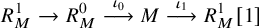(2.1) $$ \begin{align} R^1_M\to R^0_M\overset{\iota_0}{\longrightarrow}M\overset{\iota_1}{\longrightarrow}R^1_M[1] \end{align} $$

with $R^0_M, R^1_M\in \operatorname {add} R$ . Since R is rigid, we have that $\iota _0$ is a right $\operatorname {add} R$ -approximation of M and $\iota _1$ is a left $\operatorname {add} R[1]$ -approximation of M. Moreover, in (2.1), $\iota _0$ can be chosen to be right minimal, or equivalently, $\iota _1$ can be chosen to be left minimal. In such case, we call (2.1) a minimal R-presentation.

Proposition 2.2. If (2.1) is a minimal R-presentation, then $R^1_M$ and $R^0_M$ do not have an indecomposable direct summand in common.

Proof. The proof of [21, Proposition 2.1] also works here.

2.1 Rigid objects in two-term subcategories

Throughout the rest of this section, let R be a basic rigid object in $\mathcal {D}$ . We introduce the notion of maximal rigid objects with respect to $R\ast R[1]$ .

Definition 2.3. An object $U\in R\ast R[1]$ is called maximal rigid with respect to $R\ast R[1]$ provided that it is rigid and for any object $N\in R\ast R[1]$ with $N\,{\oplus}\, U$ rigid, we have $N\in \operatorname {add} U$ .

Denote by $\operatorname {rigid-}(R\ast R[1])$ the set of (isoclasses of) basic rigid objects in $R\ast R[1]$ , and by $\operatorname {max}\operatorname {rigid-}(R\ast R[1])$ the set of (isoclasses of) basic maximal rigid objects with respect to $R\ast R[1]$ .

In the case that R is maximal rigid (resp. cluster tilting), by [54, Corollary 2.5], any rigid object in $\mathcal {D}$ also belongs to $R\ast R[1]$ . Therefore, the maximal rigid objects with respect to $R\ast R[1]$ are exactly the maximal rigid (resp. cluster tilting) objects in $\mathcal {D}$ .

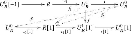
Lemma 2.4. For any $U\in \operatorname {max}\operatorname {rigid-}(R\ast R[1])$ , we have $R\in \operatorname {rigid-}(U[-1]\ast U)$ . For any triangle

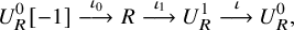(2.2) $$ \begin{align} U^0_R[-1]\overset{\iota_0}{\longrightarrow}R\overset{\iota_1}{\longrightarrow}U^1_R\overset{\iota}{\longrightarrow}U^0_R, \end{align} $$

the following hold.

1. (1) If $\iota _0$ is a right $\operatorname {add} U[-1]$ -approximation of R, then $U^1_R\in \operatorname {add} U$ .

2. (2) If $\iota _1$ is a left $\operatorname {add} U$ -approximation of R, then $U^0_R\in \operatorname {add} U$ .

Proof. Due to the existence of right $\operatorname {add} U[-1]$ -approximations of R, the assertion (1) implies $R\in \operatorname {rigid-}(U[-1]\ast U)$ . Similarly, the assertion (2) implies $R\in \operatorname {rigid-}(U[-1]\ast U)$ , too. So it suffices to show (1) and (2). We only prove (1) since (2) can be proved dually.

Since $\iota _0$ is a right $\operatorname {add} U[-1]$ -approximation, we have $U^0_R\in \operatorname {add} U$ . Since $U\in R\ast R[1]$ and $R\ast R[1]$ is closed under taking direct summands, we have $U^0_R\in R\ast R[1]$ . Hence, $U^1_R\in R\ast U^0_R\subseteq R\ast R[1]$ . Applying $\operatorname {Hom}(U[-1],-)$ to the triangle (2.2), we get a long exact sequence in $\mathcal {D}$

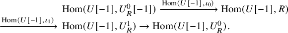$$\begin{align*}\begin{array}{rl} &\operatorname{Hom}(U[-1],U^0_R[-1])\xrightarrow{\operatorname{Hom}(U[-1],\iota_0)}\operatorname{Hom}(U[-1],R)\\ \xrightarrow{\operatorname{Hom}(U[-1],\iota_1)}&\operatorname{Hom}(U[-1],U^1_R) \to \operatorname{Hom}(U[-1],U^0_R). \end{array}\end{align*}$$

Since U is rigid, the last term $\operatorname {Hom}(U[-1],U^0_R)=0$ . Since $\iota _0$ is a right $\operatorname {add} U[-1]$ -approximation of R, the morphism $\operatorname {Hom}(U[-1],\iota _0)$ is surjective. So $\operatorname {Hom}(U[-1],U^1_R)=0$ , which implies $\operatorname {Hom}(U^1_R,U[1])=0$ by the 2-Calabi-Yau property. In particular, $\operatorname {Hom}(U^1_R,U^0_R[1])=0$ .

For any $f\in \operatorname {Hom}(U^1_R,U^1_R[1])$ , consider the following diagram.

Since $\iota [1]\circ f\in \operatorname {Hom}(U^1_R,U^0_R[1])=0$ , there exists $f_1\in \operatorname {Hom}(U^1_R,R[1])$ such that $f=\iota _1[1]\circ f_1$ . Since $f_1\circ \iota _1\in \operatorname {Hom}(R,R[1])=0$ , there exists $f_2\in \operatorname {Hom}(U^0_R,R[1])$ such that $f_1=f_2\circ \iota $ . Since $\iota _0[1]$ is a right $\operatorname {add} U$ -approximation of $R[1]$ , there exists $f_3\in \operatorname {Hom}(U^0_R,U^0_R)$ such that $f_2=(\iota _0[1])f_3$ . Hence, we have $f=\iota _1[1]\circ \iota _0[1]\circ f_3\circ \iota $ , which is zero since $\iota _1[1]\circ \iota _0[1]=0$ . So $U^1_R$ is rigid, and hence $\operatorname {Hom}((U^1_R\,{\oplus}\, U),(U^1_R\,{\oplus}\, U)[1])=0$ . Since U is maximal rigid with respect to $R\ast R[1]$ , we have $U^1_R\in \operatorname {add} U$ .

We use $K_0^{\mbox {sp}}(R)$ to denote the split Grothendieck group of $\operatorname {add} R$ . For any $M\in R\ast R[1]$ , define the index of M with respect to R as the element in $K_0^{\mbox {sp}}(R)$

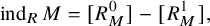(2.3) $$ \begin{align} \operatorname{ind}_RM=[R^0_M]-[R^1_M], \end{align} $$

where $R^1_M\to R^0_M\to M\to R^1_M[1]$ is an R-presentation of M. We write $R=\,{\oplus}\, ^n_{i=1}R_i$ with $R_i$ indecomposable. Then $[R_i],1\leq i\leq n$ , form a $\mathbb {Z}$ -basis of $K_0^{\mbox {sp}}(R)$ . Denote by $[\operatorname {ind}_R M:R_i]$ the coefficient of $[R_i]$ in the decomposition of $\operatorname {ind}_RM$ with respect to this basis. Then we have

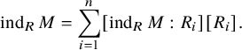$$ \begin{align*}\operatorname{ind}_RM=\sum_{i=1}^{n}[\operatorname{ind}_RM:R_i][R_i].\end{align*} $$

Remark 2.5. We refer to [21, Section 2.3], [47, Section 2.1] and [48, Section 2.5] for a similar definition of the index with respect to cluster tilting objects. Moreover, if R is a direct summand of a cluster tilting object T, then for any object $M\in \mathcal {D}$ , we have $M\in R\ast R[1]$ if and only if $[\operatorname {ind}_T M:X]=0$ for any indecomposable direct summand X of $T\setminus R$ .

Proposition 2.6. Let $U=\,{\oplus}\, ^m_{i=1}U_i$ be a basic rigid object in $R\ast R[1]$ with $U_i, 1\leq i\leq m$ , indecomposable. Then the elements $\operatorname {ind}_RU_i, 1\leq i\leq m$ , are linearly independent in $K_0^{\mbox {sp}}(R)$ .

Proof. The proof of [21, Theorem 2.4] also works here.

We have the following criterion of a rigid object in $R\ast R[1]$ to be maximal rigid with respect to $R\ast R[1]$ by counting rank.

Proposition 2.7. For any $U\in \operatorname {rigid-}(R\ast R[1])$ , we have $|U|\leq |R|$ , where equality holds if and only if $U\in \operatorname {max}\operatorname {rigid-}(R\ast R[1])$ .

Proof. Let $U=\,{\oplus}\, ^m_{i=1}U_i$ be a basic rigid object in $R\ast R[1]$ with $U_i,1\leq i\leq m$ , indecomposable. By Proposition 2.6, we have

$$\begin{align*}|U|=\operatorname{rank}\{\operatorname{ind}_RU_j|1\leq j\leq m\}\leq\operatorname{rank}\{\operatorname{ind}_R R_i|1\leq i\leq n\}=|R|,\end{align*}$$

where $\operatorname {rank} X$ denotes the rank of a set $X\subseteq K_0^{\mbox {sp}}(R)$ .

Let U be a maximal rigid object with respect to $R\ast R[1]$ . On the one hand, U is rigid in $R\ast R[1]$ , which implies $|U|\leq |R|$ . On the other hand, by Lemma 2.4, we have $R\in \operatorname {rigid-}(U[-1]\ast U)$ , which implies $|R|\leq |U|$ . Hence, we have $|R|=|U|$ . Conversely, let $U\in \operatorname {rigid-}(R\ast R[1])$ with $|U|=|R|$ . For any $N\in R\ast R[1]$ such that $U\,{\oplus}\, N$ is rigid, we have $|U\,{\oplus}\, N|\leq |R|$ . Then $|U|=|U\,{\oplus}\, N|$ , which implies $N\in \operatorname {add} U$ . So U is maximal rigid with respect to $R\ast R[1]$ .

As a consequence of Lemma 2.4 and Proposition 2.7, we have the following dual relation between two rigid objects.

Corollary 2.8. Let U and R be rigid objects in $\mathcal {D}$ . Then $U\in \operatorname {max}\operatorname {rigid-}(R\ast R[1])$ if and only if $R\in \operatorname {max}\operatorname {rigid-}(U[-1]\ast U)$ .

Proof. For any $U\in \operatorname {max}\operatorname {rigid-}(R\ast R[1])$ , by Lemma 2.4, we have $R\in \operatorname {rigid-}(U[-1]\ast U)$ , and by Proposition 2.7, we have $|U|=|R|$ . Then $|R|=|U[-1]|$ . So by Proposition 2.7 again, we have $R\in \operatorname {max}\operatorname {rigid-}(U[-1]\ast U)$ . The opposite implication can be obtained by switching R with $U[-1]$ .

The following lemma is useful.

Lemma 2.9. Let U and R be basic rigid objects in $\mathcal {D}$ . If $R\in \operatorname {max}\operatorname {rigid-}(U[-1]\ast U)$ , then for any indecomposable summand Y of U, we have $[\operatorname {ind}_{U[-1]}R:Y[-1]]\neq 0$ .

Proof. Let $N=U\setminus Y$ . If $[\operatorname {ind}_{U[-1]}R:Y[-1]]= 0$ then by the definition of index, R admits an $N[-1]$ -presentation. So by Proposition 2.7, we have $|R|\leq |N|<|U|$ . Since $R\in \operatorname {max}\operatorname {rigid-}(U[-1]\ast U)$ , again by Proposition 2.7, we have $|R|=|U|$ , a contradiction.

2.2 Mutation in two-term subcategories

By Proposition 2.7, any rigid object in $R\ast R[1]$ can be completed to a maximal rigid object with respect to $R\ast R[1]$ .

Definition 2.10. A basic rigid object N in $R\ast R[1]$ is called almost maximal rigid with respect to $R\ast R[1]$ if $|N|=|R|-1$ .

Let N be an almost maximal rigid object with respect to $R\ast R[1]$ . An indecomposable object Y is called a completion of N if $N\,{\oplus}\, Y$ is maximal rigid with respect to $R\ast R[1]$ .

Lemma 2.11. Let N be an almost maximal rigid object with respect to $R\ast R[1]$ , and $Y,Y^{\prime }$ be two non-isomorphic completions of N. Then

$$ \begin{align*}[\operatorname{ind}_{(Y^{\prime}\,{\oplus}\, N)[-1]}R:Y^{\prime}[-1]][\operatorname{ind}_{(Y\,{\oplus}\, N)[-1]}R:Y[-1]]<0.\end{align*} $$

Proof. Let $[\operatorname {ind}_{(Y\,{\oplus}\, N)[-1]}R:Y[-1]]=t$ and $[\operatorname {ind}_{(Y^{\prime }\,{\oplus}\, N)[-1]}R:Y^{\prime }[-1]]=s.$ Assume conversely $ts\geq 0$ . By Lemma 2.9, we have $t\neq 0$ and $s\neq 0$ . So either $t<0$ and $s<0$ , or and . We only make a contradiction for the case $t<0$ and $s<0$ since the other case is similar. Let $U=N\,{\oplus}\, Y$ and $U^{\prime }=N\,{\oplus}\, Y^{\prime }$ . Consider the following diagram

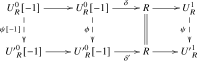
where the first (resp. second) row is a minimal $U[-1]$ -presentation (resp. $U^{\prime }[-1]$ -presentation) of R. Since $t<0$ and $s<0$ , by Proposition 2.2, both $U_R^0$ and ${U^{\prime }}^0_R$ belong to $\operatorname {add} N$ , and Y and $Y^{\prime }$ are direct summands of $U^1_R$ and ${U^{\prime }}^1_R$ , respectively. So both $\delta $ and $\delta ^{\prime }$ are minimal right $\operatorname {add} N[-1]$ -approximations of R. Hence, there exists an isomorphism $\phi :U_R^0[-1]\to {U^{\prime }}^0_R[-1]$ such that the middle square of the above diagram commutes. It follows that there exists an isomorphism $\psi :U_R^1\to {U^{\prime }}_R^1$ , and hence, $Y\cong Y^{\prime }$ , a contradiction.

It follows from Lemma 2.11 that any almost maximal rigid object with respect to $R\ast R[1]$ has at most two completions. In what follows, we shall prove that the number of completions is exactly two. For this, we need the following notion of left/right mutation of a basic rigid object in $\mathcal {D}$ at an indecomposable summand, introduced in [35, Definition 2.5].

Definition 2.12. Let $U=N\,{\oplus}\, Y$ be a basic rigid object in $\mathcal {D}$ , with Y an indecomposable direct summand of U. The right mutation $\mu ^+_Y(U)=N\,{\oplus}\, Z$ and the left mutation $\mu ^-_Y(U)=N\,{\oplus}\, W$ of U at Y are defined respectively by the triangles

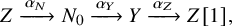(2.4) $$ \begin{align} Z\xrightarrow{\alpha_N}N_0\xrightarrow{\alpha_Y}Y\xrightarrow{\alpha_Z}Z[1], \end{align} $$

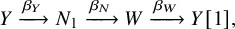(2.5) $$ \begin{align} Y\xrightarrow{\beta_Y}N_1\xrightarrow{\beta_N}W\xrightarrow{\beta_W}Y[1], \end{align} $$

where $\alpha _Y$ and $\beta _Y$ are minimal right and left $\operatorname {add} N$ -approximations of Y, respectively. The triangles (2.4) and (2.5) are called the right and left exchange triangles of U at Y, respectively.

In Definition 2.12, both Z and W are indecomposable and not isomorphic to Y, both $\mu ^+_Y(U)$ and $\mu ^-_Y(U)$ are rigid, and $|\mu ^+_Y(U)|=|\mu ^-_Y(U)|=|U|$ ; cf. [44, Section 2.1]. Hence, by Proposition 2.7, we have the following result.

Lemma 2.13. Let U be a basic rigid object in $\mathcal {D}$ , with Y an indecomposable direct summand of U. If U is a basic maximal rigid object with respect to $R\ast R[1]$ , then so is $\mu ^\varepsilon _Y(U)$ , provided that it is in $R\ast R[1]$ , where $\varepsilon \in \{+,-\}$ .

Note that any of $\mu ^+_Y(U)$ and $\mu ^-_Y(U)$ may not be in $R\ast R[1]$ .

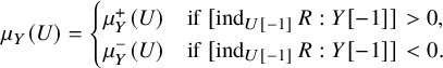
Proposition 2.14. Let $U=N\,{\oplus}\, Y\in \operatorname {max}\operatorname {rigid-}(R\ast R[1])$ and Y be an indecomposable summand of U. We use the triangles (2.4) and (2.5). The following are equivalent.

1. (1) .

2. (2) $\operatorname {Hom}(R,\alpha _Y)$ is surjective.

3. (3) $\mu ^+_Y(U)\in \operatorname {max}\operatorname {rigid-}(R\ast R[1])$ and $[\operatorname {ind}_{\mu ^+_Y(U)[-1]}R:Z[-1]]<0$ .

Dually, the following are equivalent.

1. (1’) $[\operatorname {ind}_{U[-1]}R:Y[-1]]<0$ .

2. (2’) $\operatorname {Hom}(\beta _Y,R[1])$ is surjective.

3. (3’) $\mu ^-_Y(U)\in \operatorname {max}\operatorname {rigid-}(R\ast R[1])$ and .

Proof. We only prove the equivalences between (1), (2) and (3), since the equivalences between (1’), (2’) and (3’) can be proved dually.

$(1)\Rightarrow (2)$ . Take a minimal $U[-1]$ -presentation of R:

$$\begin{align*}U^1_R[-1]\longrightarrow U^0_R[-1]\xrightarrow{\iota_0} R\xrightarrow{\iota_1} U^1_R.\end{align*}$$

Since $\iota _1$ is a left $\operatorname {add} U$ -approximation of R, for any morphism $g\in \operatorname {Hom}(R,Y)$ , there exists $h\in \operatorname {Hom}(U^1_R,Y)$ such that $g=h\circ \iota _1$ . Since , by Proposition 2.2, we have $U^1_R\in \operatorname {add} N$ . Since $\alpha _Y$ is a right $\operatorname {add} N$ -approximation of Y, there exists $h^{\prime }\in \operatorname {Hom}(U^R_1,N_0)$ such that $h=\alpha _Y\circ h^{\prime }$ . Then we have $g=\alpha _Y\circ h^{\prime }\circ \iota _1$ , which implies $\operatorname {Hom}(R,\alpha _Y)$ is surjective.

$(2)\Rightarrow (3)$ . Let

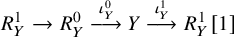$$\begin{align*}R^1_Y\to R^0_Y\overset{\iota^0_Y}{\longrightarrow}Y\overset{\iota^1_Y}{\longrightarrow} R^1_Y[1]\end{align*}$$

be a minimal R-presentation of Y. Since $\operatorname {Hom}(R,\alpha _Y)$ is surjective, there exists $\iota ^{\prime }_0\in \operatorname {Hom}(R^0_Y,N_0)$ such that $\iota ^0_Y=\alpha _Y\circ \iota ^{\prime }_0$ . So by the octahedral axiom, we have the following commutative diagram of triangles.

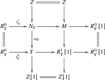
Since $M\in N_0\ast R^0_Y[1]\subseteq R\ast R[1]$ , we have $Z\in R^1_Y\ast M\subseteq R\ast R[1]$ . Thus, by Lemma 2.13, we have $\mu ^+_Y(U)=N\,{\oplus}\, Z\in \operatorname {max}\operatorname {rigid-}(R\ast R[1])$ .

Applying $\operatorname {Hom}(R,-)$ to the right exchange triangle (2.4), we have the following exact sequence:

$$\begin{align*}\operatorname{Hom}(R,N_0)\xrightarrow{\operatorname{Hom}(R,\alpha_Y)}\operatorname{Hom}(R,Y)\longrightarrow\operatorname{Hom}(R,Z[1])\xrightarrow{\operatorname{Hom}(R,\alpha_N[1])}\operatorname{Hom}(R,N_0[1]).\end{align*}$$

Since $\operatorname {Hom}(R,\alpha _Y)$ is surjective, we have $\operatorname {Hom}(R,\alpha _N[1])$ is injective. So by the 2-Calabi-Yau property, the morphism $\operatorname {Hom}(\alpha _N,R[1])$ is surjective. Hence, any $g\in \operatorname {Hom}(Z[-1],R)$ factors through $N_0[-1]$ . So any right $\operatorname {add} N[-1]$ -approximation of R is also a right $\operatorname {add}\mu ^+_Y(U)[-1]$ -approximation of R. By Lemma 2.9, it follows that $[\operatorname {ind}_{\mu ^+_Y(U)[-1]}R:Z[-1]]<0$ .

$(3)\Rightarrow (1)$ . Since $Z\not \cong Y$ , this implication follows from Lemma 2.11 directly.

Now we are ready to show that each almost maximal rigid object with respect to $R\ast R[1]$ has exactly two completions.

Theorem 2.15. Let N be an almost maximal rigid object with respect to $R\ast R[1]$ . Then there are exactly two complements Y and $Y^{\prime }$ of N. Moreover, we have

$$ \begin{align*}[\operatorname{ind}_{(N\,{\oplus}\, Y)[-1]}R:Y[-1]][\operatorname{ind}_{(N\,{\oplus}\, Y^{\prime})[-1]}R:Y^{\prime}[-1]]<0.\end{align*} $$

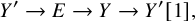
In the case and $[\operatorname {ind}_{(N\,{\oplus}\, Y^{\prime })[-1]}R:Y^{\prime }[-1]]<0$ , there is a triangle

$$ \begin{align*}Y^{\prime}\to E\to Y\to Y^{\prime}[1],\end{align*} $$

with $E\in \operatorname {add} N$ , and which under the functor $\operatorname {Hom}(R,-)$ becomes an exact sequence

$$ \begin{align*}\operatorname{Hom}(R,Y^{\prime})\to\operatorname{Hom}(R,E)\to\operatorname{Hom}(R,Y)\to 0.\end{align*} $$

Proof. By Proposition 2.7, there is a completion X of N. By Lemma 2.9, we have $[\operatorname {ind}_{(N\,{\oplus}\, X)[-1]}R:X[-1]]\neq 0$ . If , we take $Y=X$ and $Y^{\prime }=\mu ^+_X(N\,{\oplus}\, X)\setminus N$ . Then by Proposition 2.14, the triangle (2.4) becomes the required one. If $[\operatorname {ind}_{(N\,{\oplus}\, X)[-1]}R:X[-1]]<0$ , we take $Y^{\prime }=X$ and $Y=\mu ^-_{X}(N\,{\oplus}\, X)\setminus N$ . Then by Proposition 2.14, the triangle (2.5) becomes the required one.

An alternative description of Theorem 2.15 is the following mutation version.

Corollary 2.16. Let $U\in \operatorname {max}\operatorname {rigid-}(R\ast R[1])$ and Y be an indecomposable summand of U. Then there is a unique (up to isomorphism) object $\mu _Y(U)$ in $\operatorname {max}\operatorname {rigid-}(R\ast R[1])$ such that $\mu _Y(U)$ contains $U\setminus Y$ as a direct summand and is not isomorphic to U. Moreover,

Remark 2.17. By Proposition 2.2, (resp. $<0$ ) if and only if (resp. $<0$ ) for some indecomposable direct summand G of R.

2.3 Compatibility with $\tau $ -tilting theory

In this subsection, we show that the mutation in $\operatorname {max}\operatorname {rigid-}(R\ast R[1])$ is compatible with the mutation of $\tau $ -tilting pairs over the endomorphism algebra $\operatorname {End} R$ .

We briefly recall the $\tau $ -tilting theory from [1]. Let $\Lambda $ be a finite-dimensional algebra. Denote by $\operatorname {mod}\Lambda $ the category of finitely generated right $\Lambda $ -modules, and by $\tau $ the Auslander-Reiten translation in $\operatorname {mod}\Lambda $ . For any $M\in \operatorname {mod}\Lambda $ , we denote by $\operatorname {Fac}(M)$ the subcategory of $\operatorname {mod}\Lambda $ consisting of factor modules of direct sums of copies of M.

Definition 2.18. Let $M,P\in \operatorname {mod}\Lambda $ with P projective.

1. (1) The module M is called $\tau $ -rigid if $\operatorname {Hom}_{\Lambda }(M,\tau M)=0$ .

2. (2) The pair $(M,P)$ is called a $\tau $ -rigid pair if M is $\tau $ -rigid and $\operatorname {Hom}_{\Lambda }(P,M)=0$ .

3. (3) The pair $(M,P)$ is called a $\tau $ -tilting pair if it is a $\tau $ -rigid pair and $|M|+|P|=|\Lambda |$ . In this case, M is called a support $\tau $ -tilting module.

4. (4) The pair $(M,P)$ is called an almost complete $\tau $ -tilting pair if it is a $\tau $ -rigid pair and $|M|+|P|=|\Lambda |-1$ . In this case, M is called an almost complete support $\tau $ -tilting module.

For any basic support $\tau $ -tilting module M, there is a unique P (up to isomorphism) such that $(M,P)$ is a basic $\tau $ -tilting pair. Hence, one can identify basic support $\tau $ -tilting modules with basic $\tau $ -tilting pairs. There is a partial order on the set of basic support $\tau $ -tilting modules, given by $M\geq N$ if and only if $N\in \operatorname {Fac} M$ .

Theorem 2.19 [1, Theorem 2.18 and Definition-Proposition 2.28]

Any basic almost complete $\tau $ -tilting pair $(N,Q)$ is a direct summand of exactly two non-isomorphic basic $\tau $ -tilting pairs $(M,P)$ and $(M^{\prime },P^{\prime })$ . Moreover, either or .

In the setting of Theorem 2.19, suppose . Then $(M,P)$ is called the right mutation of $(M^{\prime },P^{\prime })$ at $(N,Q)$ and denote $(M,P)=\mu ^+_{(N,Q)}(M^{\prime },P^{\prime })$ . Dually, $(M^{\prime },P^{\prime })$ is called the left mutation of $(M,P)$ at $(N,Q)$ and denote $(M^{\prime },P^{\prime })=\mu ^-_{(N,Q)}(M,P)$ .

Definition 2.20. The exchange graph $\operatorname {EG}(\operatorname {s\tau -tilt}\Lambda )$ of support $\tau $ -tilting modules over $\Lambda $ has basic $\tau $ -tilting pairs as vertices and has mutations as edges.

Let $\Lambda _R=\operatorname {End} R$ . The following result establishes a link between $R\ast R[1]$ and $\operatorname {mod}\Lambda _R$ .

Theorem 2.21 [35, Proposition 6.2], [18, Proposition 2.2, Theorem 3.2]

The functor $\operatorname {Hom}(R,-):\mathcal {D}\to \operatorname {mod}\Lambda _R$ induces an equivalence

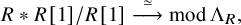$$\begin{align*}R\ast R[1]/R[1]\overset{\simeq}{\longrightarrow}\operatorname{mod}\Lambda_R,\end{align*}$$

such that for any $X\in R\ast R[1]$ without nonzero common direct summands with $R[1]$ , we have

$$\begin{align*}\tau\operatorname{Hom}(R,X)=\operatorname{Hom}(R,X[1]).\end{align*}$$

Moreover, this equivalence induces a bijection

$$\begin{align*}\begin{array}{rccc} \Phi\colon & \operatorname{rigid-}(R\ast R[1]) & \to & \operatorname{\tau-rigidp}\operatorname{mod}\Lambda_R \\ & X_1\,{\oplus}\, X_2 & \mapsto & (\operatorname{Hom}(R,X_1),\operatorname{Hom}(R,X_2[-1])) \end{array} \end{align*}$$

where $\operatorname {\tau -rigidp}\operatorname {mod}\Lambda _R$ is the set of (isoclasses of) basic $\tau $ -rigid pairs in $\operatorname {mod}\Lambda _R$ , $X_2\in \operatorname {add} R[1]$ and $X_1$ has no nonzero common direct summands with $R[1]$ . This bijection restricts to a bijection from $\operatorname {max}\operatorname {rigid-}(R\ast R[1])$ to the set of (isoclasses of) basic $\tau $ -tilting pairs.

This allows us to apply our results of mutation on $R\ast R[1]$ to the $\tau $ -tilting theory in $\operatorname {mod}\Lambda _R$ .

Theorem 2.22. For any $U=N\,{\oplus}\, Y\in \operatorname {max}\operatorname {rigid-}(R\ast R[1])$ with Y an indecomposable summand of U, we have

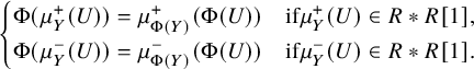$$\begin{align*}\begin{cases} \Phi(\mu^+_Y(U))=\mu^+_{\Phi(Y)}(\Phi(U))&\text{if} \mu^+_Y(U)\in R\ast R[1],\\ \Phi(\mu^-_Y(U))=\mu^-_{\Phi(Y)}(\Phi(U))&\text{if} \mu^-_Y(U)\in R\ast R[1]. \end{cases}\end{align*}$$

Proof. Let $Y^{\prime }$ be another completion of N. If $\mu ^+_Y(U)\in R\ast R[1]$ , then it is maximal rigid with respect to $R\ast R[1]$ by Lemma 2.13. So by Corollary 2.16, we have $\mu ^+_Y(U)=N\,{\oplus}\, Y^{\prime }$ and . Then by Theorem 2.15, there is a triangle

$$ \begin{align*}Y^{\prime}\to E\to Y\to Y^{\prime}[1],\end{align*} $$

with $E\in \operatorname {add} N$ and such that there is an exact sequence

$$ \begin{align*}\operatorname{Hom}(R,Y^{\prime})\to\operatorname{Hom}(R,E)\to\operatorname{Hom}(R,Y)\to 0.\end{align*} $$

In particular, we have $\operatorname {Hom}(R,U)\in \operatorname {Fac}\operatorname {Hom}(R,N)\subseteq \operatorname {Fac}\operatorname {Hom}(R,\mu ^+_Y(U))$ . By definition, we have , which implies $\Phi (\mu ^+_Y(U))=\mu ^+_{\Phi (Y)}(\Phi (U))$ , as required. The case $\mu ^-_Y(U)\in R\ast R[1]$ can be proved dually.

2.4 Relations with reductions

Let G be a rigid object in $\mathcal {D}$ . Denote by $\mathcal {D}_G={}^{\perp }G[1]/ {\langle } \operatorname {add} G{\rangle }$ the quotient of the full subcategory ${}^{\perp }G[1]$ by the ideal ${\langle }\operatorname {add} G{\rangle }$ consisting of morphisms that factor through objects in $\operatorname {add} G$ . For any morphism f in ${}^{\perp }G[1]$ , denote by $\bar {f}$ the image of f in the quotient $\mathcal {D}_G$ .

Theorem 2.23 [35, Theorem 4.2]

The category $\mathcal {D}_G$ is a triangulated category whose suspension functor ${\langle }1{\rangle }_G$ and its inverse ${\langle }-1{\rangle }_G$ are given by the triangles in $\mathcal {D}$

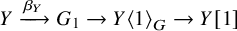$$\begin{align*}Y\xrightarrow{\beta_Y}G_1\to Y{\langle}1{\rangle}_G\to Y[1]\end{align*}$$

and

$$\begin{align*}Y[-1]\to Y{\langle}-1{\rangle}_G\to G_0\xrightarrow{\alpha_Y}Y,\end{align*}$$

respectively, where $\beta _Y$ (resp. $\alpha _Y$ ) is a left (resp. right) $\operatorname {add} G$ -approximation of Y. The triangles in $\mathcal {D}_G$ are isomorphic to

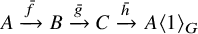$$\begin{align*}A\xrightarrow{\bar{f}} B\xrightarrow{\bar{g}} C\xrightarrow{\bar{h}} A{\langle}1{\rangle}_G\end{align*}$$

induced by the following diagram of triangles in $\mathcal {D}$ :

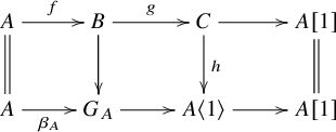
with $A,B,C\in {}^{\perp }G[1]$ .

We simply denote ${\langle }1{\rangle }={\langle }1{\rangle }_G$ and ${\langle }-1{\rangle }={\langle }-1{\rangle }_G$ , if there is no confusion arising.

Remark 2.24. Let $U=N\,{\oplus}\, Y$ be a rigid object in $\mathcal {D}$ . Comparing triangles 2.4 and 2.5 with Theorem 2.23, we have $\mu ^+_Y(U)=N\,{\oplus}\, Y{\langle }-1{\rangle }_N$ and $\mu ^-_Y(U)=N\,{\oplus}\, Y{\langle }1{\rangle }_N$ .

Now consider the case that G is a direct summand of R. Denote by $\operatorname {max}\operatorname {rigid}_G\operatorname {-}(R\ast _{\mathcal {D}} R[1])$ the subset of $\operatorname {max}\operatorname {rigid-}(R\ast _{\mathcal {D}} R[1])$ consisting of those objects that admit G as a direct summand.

Proposition 2.25. Let G be a direct summand of R. Then there is a bijection

$$ \begin{align*}\Psi\colon \operatorname{max}\operatorname{rigid}_G\operatorname{-}(R\ast_{\mathcal{D}} R[1])\to\operatorname{max}\operatorname{rigid-}(R\ast_{\mathcal{D}_G} R{\langle}1{\rangle}),\end{align*} $$

sending U to $U\setminus G$ . Moreover, for any $U\in \operatorname {max}\operatorname {rigid}_G\operatorname {-}(R\ast _{\mathcal {D}} R[1])$ and any indecomposable summand Y of $U\setminus G$ , we have that $\mu ^{\varepsilon }_Y(U)\in \operatorname {max}\operatorname {rigid-}(R\ast _{\mathcal {D}} R[1])$ if and only if $\mu ^{\varepsilon }_{\Psi (Y)}(\Psi (U))\in \operatorname {max}\operatorname {rigid-}(R\ast _{\mathcal {D}_G} R{\langle }1{\rangle }),$ for any $\varepsilon \in \{+,-\}$ , and in this case, $\Psi (\mu ^{\varepsilon }_Y(U))=\mu ^{\varepsilon }_{\Psi (Y)}(\Psi (U))$ .

Proof. Let $U=G\,{\oplus}\, X$ be a basic object in $R\ast R[1]$ . By [35, Lemma 4.8], U is rigid in $\mathcal {D}$ if and only if X is rigid in ${\mathcal {D}_G}$ . Since an indecomposable object in $R\ast R[1]$ is isomorphic to zero in ${\mathcal {D}_G}$ if and only if it is isomorphic to a direct summand of G, we have $|U|=|R|$ in $\mathcal {D}$ if and only if $|X|=|R\setminus G|$ in ${\mathcal {D}_G}$ . So by Proposition 2.7, we have that $U\in \operatorname {max}\operatorname {rigid}_G\operatorname {-}(R\ast _{\mathcal {D}} R[1])$ if and only if $X\in \operatorname {max}\operatorname {rigid-}(R\ast _{\mathcal {D}_G} R{\langle }1{\rangle })$ . Thus, we get the bijection $\Psi $ .

By Theorem 2.23, a minimal U-presentation

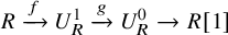$$\begin{align*}R\xrightarrow{f} U^1_R\xrightarrow{g} U^0_R\to R[1]\end{align*}$$

of $R[1]$ in $\mathcal {D}$ gives rise to a minimal X-presentation

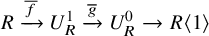$$\begin{align*}R\xrightarrow{\overline{f}} U^1_R\xrightarrow{\overline{g}} U^0_R\to R{\langle}1{\rangle}\end{align*}$$

of $R{\langle }1{\rangle }$ in ${\mathcal {D}_G}$ . So for any indecomposable summand Y of X, we have

$$ \begin{align*}[\operatorname{ind}_{U[-1]}R:Y[-1]]=[\operatorname{ind}_{U{\langle}-1{\rangle}}R:Y{\langle}-1{\rangle}].\end{align*} $$

Then for any $\varepsilon \in \{+,-\}$ , by Proposition 2.14, we have $\mu ^{\varepsilon }_Y(U)\in \operatorname {max}\operatorname {rigid}_G\operatorname {-}(R\ast _{\mathcal {D}} R[1])$ if and only if $\mu ^{\varepsilon }_{\Psi (Y)}(\Psi (U))\in \operatorname {max}\operatorname {rigid-}(R\ast _{\mathcal {D}_G} R{\langle }1{\rangle })$ . Then the last assertion follows from [35, Proposition 4.4 (2)].

3 Cluster categories arising from punctured marked surfaces

In this section, we recall the cluster categories arising from punctured marked surfaces.

3.1 Punctured marked surfaces and triangulations

We recall from [25] and [49] some notions about punctured marked surfaces.

A punctured marked surface $\mathbf {S}$ is a triple $(S,\mathbf {M},\mathbf {P})$ , where

• ○ S is a compact oriented surface with nonempty boundary $\partial S$ ,

• ○ $\mathbf {M}\subseteq \partial S$ is a finite set of marked points such that each component of $\partial S$ contains at least one marked point in $\mathbf {M}$ , and

• ○ $\mathbf {P}\subseteq (S\setminus \partial S)$ is a finite set of punctures.

Denote $\mathbf {S}^\circ :=S\setminus (\partial S\cup \mathbf {P})$ the interior of $\mathbf {S}$ . The closures of connected components in $\partial S\setminus \mathbf {M}$ are called boundary segments. Denote by B the set of boundary segments of $\mathbf {S}$ .

An arc on S is an immersion $\gamma :[0,1]\to S$ such that

1. (1) $\gamma (0),\gamma (1)\in \mathbf {M}\cup \mathbf {P}$ , $\gamma (t)\in \mathbf {S}^\circ $ for any $t\in (0,1)$ ,

2. (2) $\gamma $ is neither null-homotopic nor homotopic to a boundary segment, and

3. (3) $\gamma $ has no self-intersections in $\mathbf {S}^\circ $ .

Any arc is considered up to homotopy relative to its endpoints.

Definition 3.1 [25, Definition 2.6]

An ideal triangulation of $\mathbf {S}$ is a maximal collection of arcs on $\mathbf {S}$ that do not intersect each other in $\mathbf {S}^\circ $ .

Any ideal triangulation divides S into triangles. A triangle is called self-folded if two of its sides coincide, as shown in the left picture of Figure 1, where we use $\epsilon ^{\prime }$ to denote the folded side of a self-folded triangle whose non-folded side is $\epsilon $ . Note that the point p enclosed by $\epsilon $ is always in $\mathbf {P}$ .

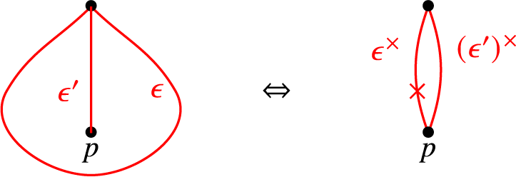
Figure 1 From ideal triangulations to tagged triangulations.

Definition 3.2. A partial ideal triangulation $\mathbf {R}$ is a subset of an ideal triangulation $\mathbf {T}$ such that for any self-folded triangle of $\mathbf {T}$ , if its non-folded side is in $\mathbf {R}$ , then so is its folded side.

Definition 3.3 [25, Definition 7.1]

A tagged arc on $\mathbf {S}$ is an arc $\gamma $ that does not cut out a once-punctured monogon by a self-intersection in $\mathbf {M}\cup \mathbf {P}$ , and is equipped with a map

$$ \begin{align*}\kappa_\gamma:\{t|\gamma(t)\in\mathbf{P}\}\to\{-1,1\}\end{align*} $$

such that $\kappa _\gamma (0)=\kappa _\gamma (1)$ if $\gamma (0)=\gamma (1)\in \mathbf {P}$ . The value $\kappa (t)$ is called the tagging of $\gamma $ at the end $\gamma (t)$ . Denote by $\operatorname {A}^\times (\mathbf {S})$ the set of tagged arcs on $\mathbf {S}$ .

In figures, we use the symbol $\times $ on one end of a tagged arc $\gamma $ to stand for that the value of $\kappa _\gamma $ at this end is taken to be $-1$ .

Remark 3.4. Each arc $\gamma $ can be viewed as a tagged arc $\gamma ^\times $ whose underlying arc is $\gamma $ and whose tagging is 1 at each punctured end.

For an arc $\epsilon $ which is a loop enclosing a puncture p, although it can not be completed to a tagged arc by adding tagging directly, we still associate a tagged arc $\epsilon ^\times $ to it, whose underlying arc is $\epsilon ^{\prime }$ , the unique arc in the interior of the once-puncture monogon enclosed by $\epsilon $ , and whose tagging is $-1$ on the end at p. See Figure 1.

Definition 3.5 [49, Definition 3.3]

Let $\gamma _1$ and $\gamma _2$ be tagged arcs in minimal position.

1. (1) Any pair $(t_1,t_2)$ with $0<t_1,t_2< 1$ and $\gamma _1(t_1)=\gamma _2(t_2)$ is called an interior intersection between $\gamma _1$ and $\gamma _2$ .

2. (2) A pair $(t_1,t_2)$ with $t_1,t_2\in \{0,1\}$ and $\gamma _1(t_1)=\gamma _2(t_2)\in \mathbf {P}$ is called a tagged intersection between $\gamma _1$ and $\gamma _2$ if the following conditions hold.

   1. (a) $\kappa _{\gamma _1}(t_1)\neq \kappa _{\gamma _2}(t_2)$ .

   2. (b) If $\gamma _1|_{t_1\to (1-t_1)}\sim \gamma _2|_{t_2\to (1-t_2)}$ , where $\gamma _i|_{t_i\to (1-t_i)}$ denotes the orientation of $\gamma _i$ from $t_i$ to $1-t_i$ , for $i=1,2$ , then $\gamma _1(1-t_1)=\gamma _2(1-t_2)\in \mathbf {P}$ and $\kappa _{\gamma _1}(1-t_1)\neq \kappa _{\gamma _2}(1-t_2)$ .

Denote by $\cap (\gamma _1,\gamma _2)$ the set of interior intersections and tagged intersections, and by $\operatorname {Int}(\gamma _1,\gamma _2)=|\cap (\gamma _1,\gamma _2)|$ the intersection number between the tagged arcs $\gamma _1$ and $\gamma _2$ .

For any two tagged arcs $\gamma _1$ and $\gamma _2$ , $\operatorname {Int}(\gamma _1,\gamma _2)=0$ if and only if they are compatible in the sense of [25, Definition 7.4].

Definition 3.6. A tagged triangulation of $\mathbf {S}$ [25, Section 7] is a maximal collection $\mathbf {T}$ of tagged arcs on $\mathbf {S}$ such that $\operatorname {Int}(\gamma _1,\gamma _2)=0$ for any $\gamma _1,\gamma _2\in \mathbf {T}$ . A partial tagged triangulation of $\mathbf {S}$ is a subset of a tagged triangulation.

Let $\mathbf {R}$ be a partial tagged triangulation of $\mathbf {S}$ . We denote by $\mathbf {P}_{\mathbf {R}}$ the subset of $\mathbf {P}$ consisting of punctures p that are endpoints of arcs in $\mathbf {R}$ . When $\mathbf {R}=\mathbf {T}$ is a tagged triangulation, we have $\mathbf {P}_{\mathbf {T}}=\mathbf {P}$ . We define a map $\kappa _{\mathbf {R}}:\mathbf {P}_{\mathbf {R}}\to \{-1,0,1\}$ as

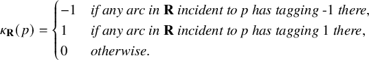$$\begin{align*}\kappa_{\mathbf{R}}(p)=\begin{cases} -1& \textit{if any arc in}\ \mathbf{R}\ \textit{incident to p has tagging}\ \text{-1}\ \textit{there},\\ 1& \textit{if any arc in}\ \mathbf{R}\ \textit{incident to p has tagging}\ \text{1}\ \textit{there},\\ 0& \textit{otherwise}. \end{cases} \end{align*}$$

Remark 3.7. Using the correspondence $\gamma \mapsto \gamma ^\times $ given in Remark 3.4, each partial ideal triangulation $\mathbf {R}$ corresponds to a partial tagged triangulation $\mathbf {R}^\times $ . By identifying $\mathbf {R}$ with $\mathbf {R}^\times $ , we regard a partial ideal triangulation $\mathbf {R}$ as a partial tagged triangulation such that $\kappa _{\mathbf {R}}(p)\geq 0$ for any $p\in \mathbf {P}_{\mathbf {R}}$ . In particular, we regard each ideal triangulation as a tagged triangulation in such a way.

Conversely, we associate a partial ideal triangulation with any partial tagged triangulation as follows.

Construction 3.8. Let $\mathbf {R}$ be a partial tagged triangulation. We construct a partial ideal triangulation $\mathbf {R}^\circ $ by

1. (1) for $p\in \mathbf {P}_{\mathbf {R}}$ with $\kappa _{\mathbf {R}}(p)\neq 0$ , removing the taggings of tagged arcs in $\mathbf {R}$ at p, and

2. (2) for $p\in \mathbf {P}_{\mathbf {R}}$ with $\kappa _{\mathbf {R}}(p)=0$ , replacing the two tagged arcs in $\mathbf {R}$ incident to p by a self-folded triangle enclosing p, as shown in Figure 1 (from right to left).

Note that when $\mathbf {R}=\mathbf {T}$ is a tagged triangulation, $\mathbf {T}^\circ $ is an ideal triangulation. For any tagged arc $\gamma \in \mathbf {R}$ , we denote by $\gamma ^{\circ _{\mathbf {R}}}$ the arc in $\mathbf {R}^\circ $ corresponding to $\gamma $ . Usually, we simply denote $\gamma ^{\circ _{\mathbf {R}}}$ by $\gamma ^{\circ }$ , when there is no confusion arising.

Note that we have $(\mathbf {R}^\times )^\circ =\mathbf {R}$ for any partial ideal triangulation $\mathbf {R}$ , but $(\mathbf {R}^\circ )^\times \neq \mathbf {R}$ for a partial tagged triangulation $\mathbf {R}$ in general, where the only difference is the taggings of arcs at $p\in \mathbf {P}_{\mathbf {R}}$ with $\kappa _{\mathbf {R}}(p)<0$ .

Construction 3.9. Let $\mathbf {R}$ be a partial tagged triangulation. For any tagged arc $\delta $ , we construct a tagged arc $\delta ^{\mathbf {R}}$ , which is obtained from $\delta $ by changing taggings at $p\in \mathbf {P}_{\mathbf {R}}$ with $\kappa _{\mathbf {R}}(p)<0$ .

Remark 3.10. For any partial tagged triangulation $\mathbf {R}$ , there exists a tagged triangulation $\mathbf {T}$ such that $\mathbf {R}\subset \mathbf {T}$ and

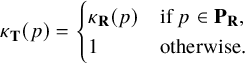$$ \begin{align*}\kappa_{\mathbf{T}}(p)=\begin{cases} \kappa_{\mathbf{R}}(p)&\text{if}\ p\in\mathbf{P}_{\mathbf{R}},\\ 1&\text{otherwise.}\end{cases}\end{align*} $$

Then we have $\gamma ^{\circ _{\mathbf {R}}}=\gamma ^{\circ _{\mathbf {T}}}$ for any $\gamma \in \mathbf {R}$ , and $\delta ^{\mathbf {T}}=\delta ^{\mathbf {R}}$ for any $\delta \in \operatorname {A}^\times (\mathbf {S})$ .

3.2 Laminates and shear coordinates

We recall from [26] (cf. also [50, 51]) the notion of laminates and their shear coordinates. The elementary laminate $e(\delta )$ of a tagged arc $\delta \in \operatorname {A}^\times (\mathbf {S})$ is defined as follows.

• ○ $e(\delta )$ is an arc running along $\delta $ in a small neighbourhood of it;

• ○ If $\delta $ has an endpoint m on $\partial S$ , then the corresponding endpoint of $e(\delta )$ is located near m on $\partial S$ in the clockwise direction as in the left picture of Figure 2;

  

  Figure 2 Elementary laminate.

• ○ If $\delta $ has an endpoint at a puncture p, then the corresponding end of $e(\delta )$ is a spiral around p clockwise (resp. anticlockwise) if $\kappa _\delta $ takes value $1$ (resp. $-1$ ) at p as in the right picture of Figure 2.

The co-elementary laminate $e^{op}(\delta )$ of $\delta $ is defined in the opposite direction.

Definition 3.11 [12, Definition 3.4]

The tagged rotation $\rho (\gamma )$ of a tagged arc $\gamma \in \operatorname {A}^\times (\mathbf {S})$ is obtained from $\gamma $ by moving each endpoint of $\gamma $ that is in $\mathbf {M}$ along the boundary anticlockwise to the next marked point and changing the tagging as $\kappa _{\rho (\gamma )}(t)=-\kappa _{\gamma }(t)$ for any t with $\gamma (t)\in \mathbf {P}$ .

Remark 3.12. For any $\delta \in \operatorname {A}^\times (\mathbf {S})$ , we have $e(\rho (\delta ))=e^{op}(\delta )$ and $e^{op}(\rho ^{-1}(\delta ))=e(\delta )$ .

Definition 3.13. Let L be the elementary laminate $e(\delta )$ or the co-elementary laminate $e^{op}(\delta )$ of a tagged arc $\delta $ . Let $\mathbf {R}$ be a partial tagged triangulation. Define $L^{\mathbf {R}}=e(\delta ^{\mathbf {R}})$ for the case $L=e(\delta )$ , and $L^{\mathbf {R}}=e^{op}(\delta ^{\mathbf {R}})$ for the case $L=e^{op}(\delta )$ , where $\delta ^{\mathbf {R}}$ is given in Construction 3.9. We call L shears $\mathbf {R}$ provided that each segment of $L^{\mathbf {R}}$ divided by arcs in $\mathbf {R}^\circ $ cuts out an angle between two arcs in $\mathbf {R}^\circ \cup B$ .

Note that when $\mathbf {R}=\mathbf {T}$ is a tagged triangulation, L always shears $\mathbf {T}$ .

Let $|\mathbf {R}|$ be the number of arcs in $\mathbf {R}$ . Using the notations in Definition 3.13, if L shears $\mathbf {R}$ , the shear coordinate vector

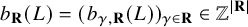$$ \begin{align*}b_{\mathbf{R}}(L)=(b_{\gamma,\mathbf{R}}(L))_{\gamma\in\mathbf{R}}\in \mathbb{Z}^{|\mathbf{R}|}\end{align*} $$

of L with respect to $\mathbf {R}$ is defined as follows.

For the case that $\mathbf {R}$ is a partial ideal triangulation, let $\gamma $ be an arc in $\mathbf {R}$ and q an intersection between $\gamma $ and L. If $\gamma $ is not the folded side of a self-folded triangle of $\mathbf {R}$ , then $\gamma $ is the common edge of the two angles of $\mathbf {R}$ that L cuts out consecutively. The contribution $b_{q,\gamma ,\mathbf {R}}(L)$ of q is defined as shown in Figure 3.

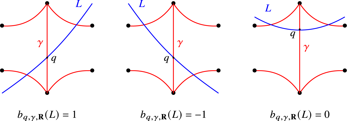
Figure 3 Contribution of an intersection q between L and $\gamma \in \mathbf {R}$ .

In this case, define

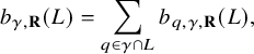$$ \begin{align*}b_{\gamma,\mathbf{R}}(L)=\sum_{q\in\gamma\cap L} b_{q,\gamma,\mathbf{R}}(L),\end{align*} $$

where $\gamma \cap L$ is the set of intersections between $\gamma $ and L. Since only finitely many q contribute nonzero values, the sum is well defined. If $\gamma =\epsilon ^{\prime }$ is the folded side of a self-folded triangle of $\mathbf {R}$ whose non-folded side is $\epsilon $ and whose enclosing puncture is p (cf. the left picture of Figure 1), define

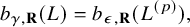$$ \begin{align*}b_{\gamma,\mathbf{R}}(L)=b_{\epsilon,\mathbf{R}}(L^{(p)}),\end{align*} $$

where $L^{(p)}$ is obtained from L by changing the directions of its spirals at p if they exist.

For the case that $\mathbf {R}$ is a partial tagged triangulation, for any $\gamma \in \mathbf {R}$ , define

$$ \begin{align*}b_{\gamma,\mathbf{R}}(L)=b_{\gamma^\circ,\mathbf{R}^{\circ}}(L^{\mathbf{R}}),\end{align*} $$

where $\mathbf {R}^\circ $ and $\gamma ^\circ $ are defined in Construction 3.8, and $L^{\mathbf {R}}$ is defined in Definition 3.13. By definition, for any tagged triangulation $\mathbf {T}$ containing $\mathbf {R}$ and for any $\gamma \in \mathbf {R}$ , we have

(3.1) $$ \begin{align} b_{\gamma,\mathbf{R}}(L)=b_{\gamma,\mathbf{T}}(L). \end{align} $$

Remark 3.14. Let $\mathbf {R}$ be a partial tagged triangulation of $\mathbf {S}$ and $\gamma \in \mathbf {R}$ . Let $\delta $ a tagged arc and let $L=e(\delta )$ or $e^{op}(\delta )$ . If there exists an intersection q between $\gamma $ and L such that $b_{q,\gamma ,\mathbf {R}}(L)=1$ (resp. $-1$ ), then for any intersection $q^{\prime }$ between $\gamma $ and L, we have $b_{q^{\prime },\gamma ,\mathbf {R}}(L)\geq 0$ (resp. $\leq 0$ ). This is because L has no self-intersections.

3.3 Cluster categories from punctured marked surfaces

A quiver is a 4-tuple $Q=(Q_0,Q_1,s,t)$ , where $Q_0$ is a set of vertices, $Q_1$ is a set of arrows, and $s,t:Q_1\to Q_0$ are the maps sending an arrow to its start and terminal, respectively. A quiver with potential is a pair $(Q,W)$ with Q a quiver and W a linear combination of cycles of Q. For more details on quivers with potential, we refer to [23].

Let $\mathbf {S}$ be a punctured marked surface. To a tagged triangulation $\mathbf {T}$ of $\mathbf {S}$ , there is an associated quiver with potential $(Q^{\mathbf {T}},W^{\mathbf {T}})$ [25, 40, 34], where $Q_0^{\mathbf {T}}$ is in bijection with $\mathbf {T}$ . By [34, Theorem 5.7], the Jacobian algebra $\Lambda ^{\mathbf {T}}$ of $(Q^{\mathbf {T}},W^{\mathbf {T}})$ is finite-dimensional and is isomorphic to

$$ \begin{align*}{\mathbf{k}} Q^{\mathbf{T}}/{\langle}\partial W^{\mathbf{T}}{\rangle},\end{align*} $$

where ${\mathbf {k}} Q^{\mathbf {T}}$ is the path algebra of $Q^{\mathbf {T}}$ over the field ${\mathbf {k}}$ and ${\langle }\partial W^{\mathbf {T}}{\rangle }$ is the ideal of ${\mathbf {k}} Q^{\mathbf {T}}$ generated by $\partial W^{\mathbf {T}}=\{\partial _a W^{\mathbf {T}}\mid a\in Q^{\mathbf {T}}_1\}$ . Then by [2], there is a ${\mathbf {k}}$ -linear, Hom-finite, Krull-Schmidt, 2-Calabi-Yau triangulated category $\mathcal {C}(Q^{\mathbf {T}},W^{\mathbf {T}})$ , called (generalized) cluster category associated to $(Q^{\mathbf {T}},W^{\mathbf {T}})$ , with a cluster tilting object $T^{\mathbf {T}}$ such that there is an equivalence of categories

$$ \begin{align*}\mathcal{C}(Q^{\mathbf{T}},W^{\mathbf{T}})/\operatorname{add} T^{\mathbf{T}}[1]\simeq\operatorname{mod}\Lambda^{\mathbf{T}}.\end{align*} $$

Moreover, by [25, 40, 34, 37], up to equivalence, the category $\mathcal {C}(Q^{\mathbf {T}},W^{\mathbf {T}})$ does not depend on the choice of the triangulation $\mathbf {T}$ . So we can use $\mathcal {C}(\mathbf {S})$ to denote this category.

Theorem 3.15 [49]

There is a bijection

$$ \begin{align*}X:\operatorname{A}^\times(\mathbf{S})\to\operatorname{ind}\operatorname{rigid}\mathcal{C}(\mathbf{S})\end{align*} $$

from the set $\operatorname {A}^\times (\mathbf {S})$ of tagged arcs on $\mathbf {S}$ to the set $\operatorname {ind}\operatorname {rigid}\mathcal {C}(\mathbf {S})$ of isoclasses of indecomposable rigid objects in $\mathcal {C}(\mathbf {S})$ , such that the following hold.

1. (1) For any $\gamma \in \operatorname {A}^\times {(\mathbf {S})}$ , we have

   $$ \begin{align*}X(\rho(\gamma))=X(\gamma)[1].\end{align*} $$

2. (2) For any tagged arcs $\gamma _1,\gamma _2$ , we have

   $$ \begin{align*}\operatorname{Int}(\gamma_1,\gamma_2)=\dim_{\mathbf{k}}\operatorname{Hom}(X(\gamma_1),X(\gamma_2)[1]).\end{align*} $$

3. (3) The bijection X induces a bijection

   $$ \begin{align*}\begin{array}{rccc} X:&\operatorname{R}^{\times}(\mathbf{S})&\to&\operatorname{rigid-}\mathcal{C}(\mathbf{S})\\ &\mathbf{R}&\mapsto&\bigoplus_{\gamma\in\mathbf{R}}X(\gamma) \end{array}\end{align*} $$
   from the set $\operatorname {R}^{\times }(\mathbf {S})$ of partial tagged triangulations of $\mathbf {S}$ to the set $\operatorname {rigid-}\mathcal {C}(\mathbf {S})$ of isoclasses of basic rigid objects in $\mathcal {C}(\mathbf {S})$ , such that $\mathbf {R}$ is a tagged triangulation if and only if $X(\mathbf {R})$ is a cluster tilting object.

4. (4) The cluster exchange graph of $\mathcal {C}(\mathbf {S})$ (i.e. the graph whose vertices are cluster tilting objects in $\mathcal {C}(\mathbf {S})$ and whose edges are mutations) is connected.

Recall from (2.3) the definition of index $\operatorname {ind}_TM$ of an object M in $\mathcal {C}(\mathbf {S})$ with respect to a cluster tilting object T.

Proposition 3.16. Let $\mathbf {T}$ be a tagged triangulation of $\mathbf {S}$ . For any tagged arc $\delta $ , we have

(3.2) $$ \begin{align} \operatorname{ind}_{X(\mathbf{T})}X(\delta)=-b_{\mathbf{T}}(e(\delta)), \end{align} $$

and

(3.3) $$ \begin{align} \operatorname{ind}_{X(\mathbf{T})[-1]}X(\delta)=-b_{\mathbf{T}}(e^{op}(\delta)). \end{align} $$

Proof. Starting from the quiver $Q^{\mathbf {T}}$ , there is a cluster algebra $\mathcal {A}$ [27]. By [25, Theorem 7.11], there is a bijection x from the set $\operatorname {A}^\times (\mathbf {S})$ of tagged arcs on $\mathbf {S}$ to the set of cluster variables of $\mathcal {A}$ , such that x induces a bijection from the set of tagged triangulations to the set of clusters of $\mathcal {A}$ , which sends $\mathbf {T}$ to the initial cluster and commutes with flips of tagged triangulations and mutations of clusters.

For the 2-Calabi-Yau category $\mathcal {C}(\mathbf {S})$ with cluster tilting object $T^{\mathbf {T}}$ , by [47] and Theorem 3.15 (4), there is a bijection $cc$ (called cluster character) from the set of indecomposable objects in $\mathcal {C}(\mathbf {S})$ to the set of cluster variables of $\mathcal {A}$ , such that $cc$ induces a bijection from the set of basic cluster tilting objects to the set of reachable clusters of $\mathcal {A}$ , which sends $T^{\mathbf {T}}$ to the initial cluster and commutes with mutations.

Then by Theorem 3.15, we have the following commutative diagram of bijections:

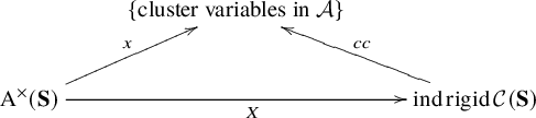
So for any tagged arc $\delta $ , $x(\delta )=cc(X(\delta ))$ . By [50, Proposition 5.2] (cf. also [41, Theorem 7.1]), the g-vector of $x(\delta )$ is $-b_{\mathbf {T}}(e(\delta ))$ . However, by [48, Proposition 3.6], the g-vector of $cc(X(\delta ))$ is $\operatorname {ind}_{T^{\mathbf {T}}}X(\delta )$ . Thus, we get (3.2).

For (3.3), we have

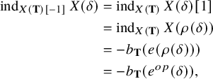$$ \begin{align*} \operatorname{ind}_{X(\mathbf{T})[-1]}X(\delta)&{}=\operatorname{ind}_{X(\mathbf{T})}X(\delta)[1]\\&=\operatorname{ind}_{X(\mathbf{T})}X(\rho(\delta)){}\\ &=-b_{\mathbf{T}}(e(\rho(\delta)))\\&=-b_{\mathbf{T}}(e^{op}(\delta)), \end{align*} $$

where the second equality holds by Theorem 3.15 (1), the third one is (3.2), and the last one is due to Remark 3.12.

Corollary 3.17. Let $\mathbf {T}$ be a tagged triangulation of $\mathbf {S}$ and $\mathbf {R}\subseteq \mathbf {T}$ . Then for any $\delta \in \operatorname {A}^\times (\mathbf {S})$ , $b_{\gamma ,\mathbf {T}}(e(\delta ))=0$ for all $\gamma \in \mathbf {T}\setminus \mathbf {R}$ if and only if $X(\delta )\in X(\mathbf {R})\ast X(\mathbf {R})[1]$ .

Proof. By Proposition 3.16, $b_{\gamma ,\mathbf {T}}(e(\delta ))=0$ if and only if $[\operatorname {ind}_{X(\mathbf {T})}X(\delta ):X(\gamma )]=0$ . Then by Remark 2.5, we get this assertion.

Corollary 3.18. Let $\mathbf {T}$ be a tagged triangulation of $\mathbf {S}$ . Then for any $\gamma ,\delta \in \mathbf {T}$ , we have

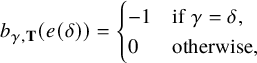$$ \begin{align*}b_{\gamma,\mathbf{T}}(e(\delta))=\begin{cases} -1&\mathrm{if}\ \gamma=\delta,\\ 0&\mathrm{otherwise,} \end{cases}\end{align*} $$

and

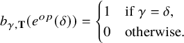$$ \begin{align*}b_{\gamma,\mathbf{T}}(e^{op}(\delta))=\begin{cases} 1&\mathrm{if}\ \gamma=\delta,\\ 0&\mathrm{otherwise.} \end{cases}\end{align*} $$

Proof. By Theorem 3.15 and the definition of index, we have

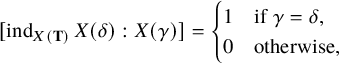$$ \begin{align*}[\operatorname{ind}_{X(\mathbf{T})}X(\delta):X(\gamma)]=\begin{cases}1&\mathrm{if}\ \gamma=\delta,\\ 0&\mathrm{otherwise,}\end{cases}\end{align*} $$

and

$$ \begin{align*}[\operatorname{ind}_{X(\mathbf{T})[-1]}X(\delta):X(\gamma)[-1]]=\begin{cases}-1&\mathrm{if}\ \gamma=\delta,\\ 0&\mathrm{otherwise.}\end{cases}\end{align*} $$

Then by Proposition 3.16, the required formulas follow.

4 A geometric model of surface rigid algebras

In this section, we give a geometric model for the module category of the endomorphism algebra of a rigid object in the cluster category of a punctured marked surface. We also show that any skew-gentle algebra is contained in this case.

Definition 4.1. A finite-dimensional algebra over ${\mathbf {k}}$ is called a surface rigid algebra if it is isomorphic to the endomorphism algebra $\Lambda _R:=\operatorname {End}_{\mathcal {C}(\mathbf {S})}R$ of a rigid object R in the cluster category $\mathcal {C}(\mathbf {S})$ of a punctured marked surface $\mathbf {S}$ .

See [20] for an unpunctured version of the above notion.

By Theorem 3.15 (3), each surface rigid algebra can be realized as the endomorphism algebra $\Lambda _{\mathbf {R}}:=\Lambda _{X(\mathbf {R})}$ of $X(\mathbf {R})$ for a partial tagged triangulation $\mathbf {R}$ of a punctured marked surface $\mathbf {S}=(S,\mathbf {M},\mathbf {P})$ .

4.1 Standard arcs and dissections

For any tagged arc $\delta \in \operatorname {A}^\times (\mathbf {S})$ whose both endpoints are in $\mathbf {P}$ , the tagged arc $\rho (\delta )=\rho ^{-1}(\delta )$ is said to be adjoint to $\delta $ .

For any partial ideal triangulation $\mathbf {R}$ of $\mathbf {S}$ and any curve $\delta $ in a minimal position with (the arcs in) $\mathbf {R}$ , an arc segment of $\delta $ (with respect to $\mathbf {R}$ ) is a segment of $\delta $ between two neighboring intersections between $\delta $ and $\mathbf {R}\cup B$ , where recall that B is the set of boundary segments of S. An arc segment of $\delta $ is called an end arc segment if it has an endpoint in $\mathbf {M}\cup \mathbf {P}$ .

Definition 4.2. Let $\mathbf {R}$ be a partial ideal triangulation of $\mathbf {S}$ . A tagged arc $\delta \in \operatorname {A}^\times (\mathbf {S})$ is called $\mathbf {R}$ -standard if and only if one of the following holds.

1. (1) $\delta \in \mathbf {R}^\times $ or $\delta $ is adjoint to some arc in $\mathbf {R}^\times $ .

2. (2) $\delta $ itself is an arc segment and cuts out an angle $\theta $ between two arcs in $\mathbf {R}\cup B$ , such that the tagging of $\delta $ has the form as shown in the first picture of Figure 4, where the left endpoint of $\delta $ is a puncture with tagging $-1$ , and the right endpoint of $\delta $ is either a marked point or a puncture with tagging $1$ .

   

   Figure 4 Arc segments of standard tagged arcs.

3. (3) $\delta $ is divided by $\mathbf {R}$ into at least two arc segments, satisfying that each arc segment $\eta $ cuts out an angle $\theta $ between two arcs in $\mathbf {R}\cup B$ (see the last three pictures of Figure 4), and in case $\eta $ having an endpoint $\mathfrak {q}$ in $\mathbf {M}\cup \mathbf {P}$ , the edge of $\theta $ with vertex $\mathfrak {q}$ is the first arc in $\mathbf {R}\cup B$ next to $\eta $ in the anticlockwise order around $\mathfrak {q}$ if $\mathfrak {q}\in \mathbf {P}$ and the tagging of $\eta $ at this end is $-1$ (see the third picture of Figure 4), or in the clockwise order otherwise (see the last picture of Figure 4).

Dually, a tagged arc $\delta \in \operatorname {A}^\times (\mathbf {S})$ is called $\mathbf {R}$ -co-standard if and only if one of the following holds.

1. (1) $\delta \in \mathbf {R}^\times $ or $\delta $ is adjoint to some arc in $\mathbf {R}^\times $ .

2. (2) $\delta $ itself is an arc segment and cuts out an angle $\theta $ between two arcs in $\mathbf {R}\cup B$ , such that the tagging of $\delta $ has the form as shown in the first picture of Figure 5, where the right endpoint of $\delta $ is a puncture with tagging $-1$ , and the left endpoint of $\delta $ is either a marked point or a puncture with tagging $1$ .

   

   Figure 5 Arc segments of co-standard tagged arcs.

3. (3) $\delta $ is divided by $\mathbf {R}$ into at least two arc segments, satisfying that each arc segment $\eta $ cuts out an angle $\theta $ between two arcs in $\mathbf {R}\cup B$ , and in case $\eta $ having an endpoint $\mathfrak {q}\in \mathbf {M}\cup \mathbf {P}$ , the edge of $\theta $ which is incident to the vertex $\mathfrak {q}$ is the first arc in $\mathbf {R}\cup B$ next to $\eta $ in the clockwise order around $\mathfrak {q}$ if $\mathfrak {q}\in \mathbf {P}$ and the tagging of $\eta $ at this end is $-1$ , or in the anticlockwise order otherwise. See the last three pictures of Figure 5.

Let $\mathbf {R}$ be a partial tagged triangulation of $\mathbf {S}$ . A tagged arc $\delta \in \operatorname {A}^\times (\mathbf {S})$ is called $\mathbf {R}$ -standard (resp. $\mathbf {R}$ -co-standard) if $\delta ^{\mathbf {R}}$ is $\mathbf {R}^\circ $ -standard (resp. $\mathbf {R}^\circ $ -co-standard). Denote by $\operatorname {A}^\times _{\mathbf {R}\operatorname {-st}}$ (resp. $\operatorname {A}^\times _{\mathbf {R}\operatorname {-co-st}}$ ) the set of $\mathbf {R}$ -standard (resp. $\mathbf {R}$ -co-standard) tagged arcs.

Remark 4.3. In Definition 4.2, since $\delta $ is a tagged arc, the two edges of $\theta $ are not from the same arc in $\mathbf {R}$ , unless in the second pictures of Figures 4 and 5, where they may be the different ends of an arc in $\mathbf {R}$ .

In the following, we give sufficient and necessary conditions on tagged arcs to be standard/co-standard.

Proposition 4.4. Let $\mathbf {R}$ be a partial tagged triangulation of $\mathbf {S}$ and $\delta $ a tagged arc. Then the following are equivalent.

1. (1) $\delta $ is $\mathbf {R}$ -standard (resp. $\mathbf {R}$ -co-standard).

2. (2) $e(\delta )$ (resp. $e^{op}(\delta )$ ) shears $\mathbf {R}$ (see Definition 3.13).

3. (3) For some/any tagged triangulation $\mathbf {T}$ such that $\mathbf {R}\subset \mathbf {T}$ , we have $b_{\gamma ,\mathbf {T}}(e(\delta ))=0$ (resp. $b_{\gamma ,\mathbf {T}}(e^{op}(\delta ))=0$ ) for any $\gamma \in \mathbf {T}\setminus \mathbf {R}$ .

4. (4) $X(\delta )\in X(\mathbf {R})\ast X(\mathbf {R})[1]$ .

Proof. We only show the equivalences between statements for the $\mathbf {R}$ -standard case, since the $\mathbf {R}$ -co-standard case can be shown dually. By Corollary 3.17, (4) is equivalent to (3). By definition, (1) is equivalent to that $\delta ^{\mathbf {R}}$ is $\mathbf {R}^\circ $ -standard, (2) is equivalent to that $e(\delta ^{\mathbf {R}})$ shears $\mathbf {R}^\circ $ . By Remark 3.10, (3) is equivalent to that for some/any tagged triangulation $\mathbf {T}$ satisfying the condition in Remark 3.10 and $\mathbf {R}\subset \mathbf {T}$ , we have $b_{\gamma ^\circ ,\mathbf {T}^\circ }(e(\delta ^{\mathbf {R}}))=0$ for any $\gamma \in \mathbf {T}\setminus \mathbf {R}$ . So we may assume that $\mathbf {R}$ is a partial ideal triangulation.

‘(1) $\Rightarrow $ (2)’: We list all the possible cases of arc segments of an $\mathbf {R}$ -standard tagged arc $\delta $ and its elementary laminate $e(\delta )$ in Figure 6, where the pictures in the first row are for $\delta \in \mathbf {R}^\times $ and $\delta ^\circ $ not a side of a self-folded triangle, those in the second row are for $\delta \in \mathbf {R}^\times $ and $\delta ^\circ $ a side of a self-folded triangle, those in the third row are for $\delta $ adjoint to $\mathbf {R}^\times $ but not in $\mathbf {R}^\times $ , those in the fourth row are for the arc segments in the first two pictures of Figure 4, and those in the last row are for the arc segments in the last two pictures of Figure 4. In each case, any segment of $e(\delta )$ cuts out an angle between two arcs in $\mathbf {R}\cup B$ . Hence, (2) holds.

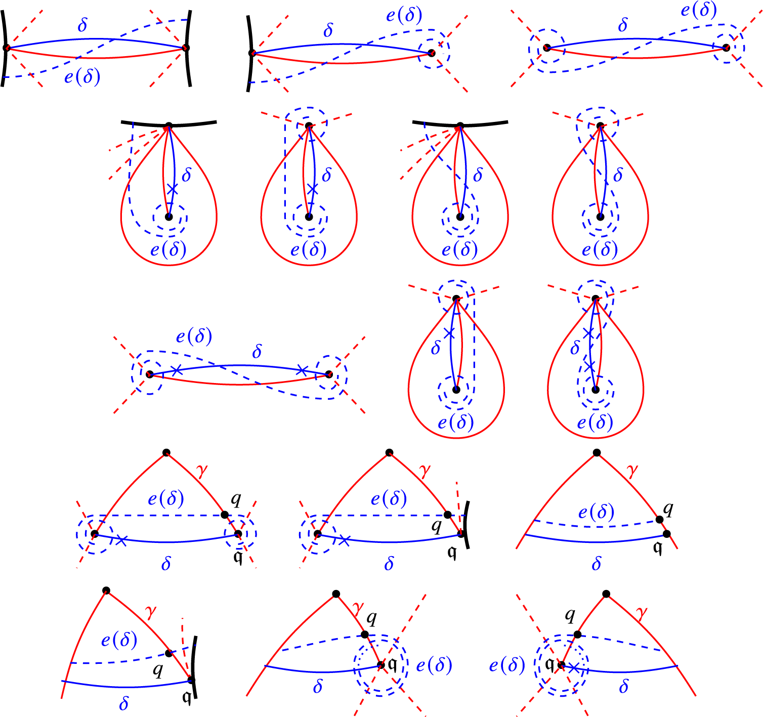
Figure 6 The elementary laminate of a standard tagged arc.

‘(2) $\Rightarrow $ (3)’: By (2), $e(\delta )$ is divided by $\mathbf {R}$ into segments, each of which cuts out an angle between two arcs in $\mathbf {R}\cup B$ . Let $\mathbf {T}$ be an ideal triangulation containing $\mathbf {R}$ , $\gamma \in \mathbf {T}\setminus \mathbf {R}$ and q an intersection between $\gamma $ and a segment $\eta $ of $e(\delta )$ . Then $\gamma $ divides the angle cut by $\eta $ into two parts. Hence, $b_{q,\gamma ,\mathbf {T}}(e(\delta ))=0$ (cf. the third picture in Figure 3). Thus, we have $b_{\gamma ,\mathbf {T}}(e(\delta ))=0$ .

‘(3) $\Rightarrow $ (1)’: If $\delta $ has no interior intersections with any arc in $\mathbf {R}$ , then we have the following three subcases.

1. (i) $\operatorname {Int}(\delta ,\gamma ^\times )=0$ for any $\gamma \in \mathbf {R}$ . Then there is a tagged triangulation $\mathbf {T}_1$ containing $\mathbf {R}^\times $ and $\delta $ . By Corollary 3.18, we have $b_{\delta ,\mathbf {T}_1}(e(\delta ))=-1$ . Hence by (3), we have $\delta \in \mathbf {R}^\times $ , which implies $\delta $ is $\mathbf {R}$ -standard.

2. (ii) Exactly one endpoint of $\delta $ , say $\delta (0)$ , is a tagged intersection with some arc in $\mathbf {R}^\times $ . Then $\delta (0)\neq \delta (1)$ . If $\kappa _\delta (0)=1$ , then there is an arc $\epsilon \in \mathbf {R}$ such that $\epsilon ^\times (0)=\delta (0)$ and $\kappa _{\epsilon ^\times }(0)=-1$ . Then $\epsilon $ is a loop enclosing $\delta (0)$ . Note that $\delta $ has no interior intersections with any arc in $\mathbf {R}$ . So $\delta $ is in the once-punctured monogon enclosed by $\epsilon $ . Thus, $\delta $ is homotopic to $\epsilon $ . Then by the definition of tagged intersections, $\delta (1)$ is also a tagged intersection between $\delta $ and $\epsilon ^\times $ , a contradiction with the setting of subsection (ii). Hence, $\kappa _\delta (0)=-1$ . Let $\delta _0$ be the tagged arc homotopic to $\delta $ and whose tagging at each tagged end is $1$ . Since $\delta _0$ has zero (if $\kappa _\delta (1)=1$ ) or two (if $\kappa _\delta (1)=-1$ ) tagged intersections with $\delta $ , there are arcs in $\mathbf {R}$ which have $\delta (0)$ as an endpoint and is not homotopic to $\delta _0$ . Take $\gamma $ to be the first arc among them next to $\delta _0$ in the anticlockwise order around $\delta (0)$ . Let $\gamma '$ be the arc or the boundary segment such that $\Delta =\{\gamma ^{\prime },\delta _0,\gamma \}$ is a (possibly self-folded) triangle with the angle from $\delta _0$ to $\gamma $ in the anticlockwise order as an inner angle. Since $\delta _0$ has no interior intersections with arcs in $\mathbf {R}$ , neither does $\gamma ^{\prime }$ . Let $\mathbf {T}_2$ be an ideal triangulation containing $\mathbf {R}$ , $\delta _0$ and $\gamma ^{\prime }$ . If $\Delta $ is self-folded, since $\gamma $ is not homotopic to $\delta $ and $\delta $ is a tagged arc (which implies that $\delta $ is not the non-folded side of a self-fold triangle), we have that $\gamma ^{\prime }$ and $\delta _0$ are folded, and $\gamma $ is the non-folded side (cf. the last picture in Figure 7). So $\delta (1)$ is a tagged intersection with either $\gamma ^\times $ (if $\kappa _\delta (1)=1$ ) or ${\gamma ^{\prime }}^\times =\delta _0$ (if $\kappa _\delta (1)=-1$ ). But since $\gamma \in \mathbf {R}$ , by Definition 3.2, we have $\gamma ^{\prime }\in \mathbf {R}$ , a contradiction with the setting of subsection (ii). Hence, the triangle $\Delta $ is not self-folded. In particular, none of $\gamma $ , $\delta _0$ and $\gamma ^{\prime }$ is the folded side of a self-folded triangle in $\mathbf {T}_2$ .

   

   Figure 7 No interior intersections but one tagged intersection.

   1. (a) If $\gamma ^{\prime }$ is a boundary segment (see the first picture in Figure 7), by Definition 4.2 (2) (see the first picture in Figure 4), $\delta $ is $\mathbf {R}$ -standard.

   2. (b) If $\gamma ^{\prime }$ is not a boundary segment and either $\delta (1)\in \mathbf {M}$ or $\delta (1)\in \mathbf {P}$ with $\kappa _\delta (1)=1$ (see the second and the third pictures in Figure 7), by definition, $b_{q,\gamma ^{\prime },\mathbf {T}_2}(e(\delta ))\neq 0$ . Then by Remark 3.14, we have $b_{\gamma ^{\prime },\mathbf {T}_2}(e(\delta ))\neq 0$ , which implies $\gamma ^{\prime }\in \mathbf {R}$ by (3). Then by Definition 4.2 (2) (see the first picture in Figure 4), $\delta $ is $\mathbf {R}$ -standard.

   3. (c) If $\delta (1)\in \mathbf {P}$ and $\kappa _\delta (1)=-1$ (see the fourth picture in Figure 7), we have $\delta =\rho (\delta _0)$ . So by Corollary 3.18, $b_{\delta _0,\mathbf {T}_2}(e(\delta ))=-1$ . Then by (3), $\delta _0\in \mathbf {R}$ , a contradiction with the setting of subsection (ii), since $\delta (1)$ is a tagged intersection between $\delta $ and $\delta ^\times _0\in \mathbf {R}^\times $ .

3. (iii) Both endpoints of $\delta $ are tagged intersections between $\delta $ and some arcs in $\mathbf {R}^\times $ . Let $\delta _0$ be the underlying arc of $\delta $ . Note that $\delta _0$ has no intersections with $\mathbf {R}$ . Let $\mathbf {T}_3$ be an ideal triangulation containing $\mathbf {R}$ and $\delta _0$ . Then $b_{\delta _0,\mathbf {T}_3}(e(\delta ))\neq 0$ by Corollary 3.18, which by (3) implies $\delta _0\in \mathbf {R}$ . So $\delta $ is adjoint to $\delta ^\times _0\in \mathbf {R}^\times $ and hence is $\mathbf {R}$ -standard.

If $\delta $ has interior intersections with some arc in $\mathbf {R}$ , then $\delta $ is divided by $\mathbf {R}$ into at least two arc segments. Let $\gamma $ be the first arc in $\mathbf {T}\cup B$ next to $\delta $ around $\delta (0)$ in the anticlockwise order if $\kappa _\delta (0)=-1$ or in the clockwise order otherwise. If $\gamma \in \mathbf {T}$ , we have $b_{\gamma ,\mathbf {T}}(e(\delta ))\neq 0$ as shown in the pictures of the last row in Figure 6. Then by (3), we have $\gamma \in \mathbf {R}$ . So the end arc segment of $\delta $ is as shown in the last two pictures in Figure 4. For any arc segment $\eta $ of $\delta $ between two arcs $\gamma _1,\gamma _2\in \mathbf {R}$ , let $\gamma ^{\prime }_0=\gamma _1,\gamma ^{\prime }_1,\cdots ,\gamma ^{\prime }_{s-1},\gamma ^{\prime }_s=\gamma _2$ be the arcs in $\mathbf {T}$ which $\eta $ crosses in order. By (3), we have $b_{\gamma ^{\prime }_i,\mathbf {T}}(e(\delta ))=0$ for any $1\leq i\leq s-1$ . Hence, $\eta $ cuts out an angle bounded by $\gamma _1$ and $\gamma _2$ (cf. the third picture in Figure 3). So $\delta $ is $\mathbf {R}$ -standard.

Remark 4.5. Let $\mathbf {R}$ be a partial ideal triangulation of $\mathbf {S}$ and $\gamma \in \mathbf {R}$ which is not the folded side of a self-folded triangle of $\mathbf {R}$ . Let $\delta $ be an $\mathbf {R}$ -standard (resp. $\mathbf {R}$ -co-standard) tagged arc which is neither in $\mathbf {R}^\times $ nor adjoint to some arc in $\mathbf {R}^\times $ , and let $L=e(\delta )$ (resp. $L=e^{op}(\delta )$ ). We denote by $\gamma \cap \alpha =\{(t_1,t_2) \mid \gamma (t_1)=\alpha (t_2) \}$ the set of intersections between $\gamma $ and $\alpha $ , where $\alpha =\delta $ or L. Note that $\gamma \cap \delta $ contains $\cap (\gamma ,\delta )$ (see Definition 3.5) as a subset. There is an injective map

$$ \begin{align*}\begin{array}{rccc} E: &\gamma\cap\delta & \to & \gamma\cap L\\ &\mathfrak{q} & \mapsto & q \\ & \end{array}\end{align*} $$

as shown in the last two rows of Figure 6 (for the case $L=e(\delta )$ ). Any intersection $q\in \gamma \cap L$ which is not in the image of E does not contribute to $b_{\gamma ,\mathbf {R}}(L)$ ; that is„ $b_{q,\gamma ,\mathbf {R}}(L)=0$ . For any $\mathfrak {q}\in \gamma \cap \delta $ and its corresponding $q\in \gamma \cap L$ , we have the following equivalences.

• ○ if and only if either $\mathfrak {q}\in \mathbf {S}^\circ $ and we are in the situation shown in the first picture of the first row of Figure 8, or $\mathfrak {q}\in \mathbf {P}$ with tagging $-1$ (resp. $\mathfrak {q}\in \mathbf {M}$ or $\mathbf {P}$ with tagging $1$ ) and $\gamma $ is the first arc in $\mathbf {R}$ next to $\delta $ anticlockwise around $\mathfrak {q}$ (see the first picture of the second (resp. third) row of Figure 8). In each case, we call $\mathfrak {q}$ positive.

  

  Figure 8 Alternative intersections of (co-)standard tagged arcs.

• ○ $b_{q,\gamma ,\mathbf {R}}(L)<0$ if and only if either $\mathfrak {q}\in \mathbf {S}^\circ $ and we are in the situation shown in the second picture of the first row of Figure 8, or $\mathfrak {q}\in \mathbf {M}$ or $\mathbf {P}$ with tagging $1$ (resp. $\mathfrak {q}\in \mathbf {P}$ with tagging $-1$ ) and $\gamma $ is the first arc in $\mathbf {R}$ next to $\delta $ clockwise around $\mathfrak {q}$ (see the second picture of the second (resp. third) row of Figure 8). In each case, we call $\mathfrak {q}$ negative.

Any positive or negative intersection $\mathfrak {q}\in \gamma \cap \delta $ is called alternative.

Definition 4.6. Let $\mathbf {R}$ be a partial tagged triangulation of $\mathbf {S}$ . An $\mathbf {R}$ -dissection (resp. $\mathbf {R}$ -co-dissection) is a maximal collection $\mathbf {U}$ of $\mathbf {R}$ -standard (resp. $\mathbf {R}$ -co-standard) arcs such that $\operatorname {Int}(\gamma _1,\gamma _2)=0$ for any $\gamma _1,\gamma _2\in \mathbf {U}$ . We denote by $D(\mathbf {R})$ (resp. $D^{op}(\mathbf {R})$ ) the set of $\mathbf {R}$ -dissections (resp. $\mathbf {R}$ -co-dissections).

By definition, any $\mathbf {R}$ -dissection is also a partial tagged triangulation of $\mathbf {S}$ .

Theorem 4.7. Let $\mathbf {R}$ be a partial tagged triangulation of $\mathbf {S}$ . The bijection X in Theorem 3.15 restricts to bijections

$$\begin{align*}X:\operatorname{A}^\times_{\mathbf{R}\operatorname{-st}}\to\operatorname{rigid-}(X(\mathbf{R})\ast X(\mathbf{R})[1])\ \textit{and}\ X:\operatorname{A}^\times_{\mathbf{R}\operatorname{-co-st}}\to\operatorname{rigid-}(X(\mathbf{R})[-1]\ast X(\mathbf{R})),\end{align*}$$

which induce bijections

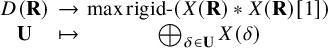(4.1) $$ \begin{align} \begin{array}{rccc} & D(\mathbf{R}) & \to & \operatorname{max}\operatorname{rigid-}(X(\mathbf{R})\ast X(\mathbf{R})[1])\\ & \mathbf{U} & \mapsto & \bigoplus_{\delta\in\mathbf{U}}X(\delta) \end{array} \end{align} $$

and

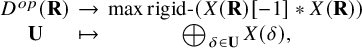(4.2) $$ \begin{align} \begin{array}{rccc} & D^{op}(\mathbf{R}) & \to & \operatorname{max}\operatorname{rigid-}(X(\mathbf{R})[-1]\ast X(\mathbf{R}))\\ & \mathbf{U} & \mapsto & \bigoplus_{\delta\in\mathbf{U}}X(\delta), \end{array} \end{align} $$

respectively. Moreover, for any $\delta \in \operatorname {A}^\times _{\mathbf {R}\operatorname {-st}}$ and any $\gamma \in \mathbf {R}$ , we have

(4.3) $$ \begin{align} [\operatorname{ind}_{X(\mathbf{R})}X(\delta):X(\gamma)]=-b_{\gamma,\mathbf{R}}(e(\delta)), \end{align} $$

and for any $\delta ^{\prime }\in \operatorname {A}^\times _{\mathbf {R}\operatorname {-co-st}}$ and any $\gamma \in \mathbf {R}$ , we have

(4.4) $$ \begin{align} [\operatorname{ind}_{X(\mathbf{R})[-1]}X(\delta^{\prime}):X(\gamma)[-1]]=-b_{\gamma,\mathbf{R}}(e^{op}(\delta^{\prime})). \end{align} $$

Proof. By the equivalence between (1) and (4) in Proposition 4.4, we get the required bijections. The last assertion then follows from Proposition 3.16 and the equality (3.1).

One consequence of the above theorem is the rank of a dissection/co-dissection.

Corollary 4.8. Let $\mathbf {R}$ be a partial tagged triangulation of $\mathbf {S}$ , and $\mathbf {U}$ a set of $\mathbf {R}$ -standard (resp. $\mathbf {R}$ -co-standard) arcs such that $\operatorname {Int}(\gamma _1,\gamma _2)=0$ for any $\gamma _1,\gamma _2\in \mathbf {U}$ . Then $\mathbf {U}$ is an $\mathbf {R}$ -dissection (resp. $\mathbf {R}$ -co-dissection) if and only if $|\mathbf {U}|=|\mathbf {R}|$ .

Proof. This follows directly from Theorem 4.7 and Proposition 2.7.

The following result tells us that dissection and co-dissection are dual notions.

Corollary 4.9. Let $\mathbf {R}$ and $\mathbf {U}$ be two partial tagged triangulations of $\mathbf {S}$ . Then $\mathbf {U}$ is an $\mathbf {R}$ -dissection if and only if $\mathbf {R}$ is a $\mathbf {U}$ -co-dissection.

Proof. By Theorem 4.7, $\mathbf {U}\in D(\mathbf {R})$ if and only if $X(\mathbf {U})\in \operatorname {max}\operatorname {rigid-}(X(\mathbf {R})\ast X(\mathbf {R})[1])$ , and $\mathbf {R}\in D^{op}(\mathbf {U})$ if and only if $X(\mathbf {R})\in \operatorname {max}\operatorname {rigid-}(X(\mathbf {U})[-1]\ast X(\mathbf {U}))$ . So the statement follows by Corollary 2.8.

The following lemma is useful in Section 5.

Lemma 4.10. Let $\mathbf {R}$ be a partial tagged triangulation of $\mathbf {S}$ , and $\mathbf {U}$ an $\mathbf {R}$ -dissection. Then for any $l\in \mathbf {U}$ , there exists $\gamma \in \mathbf {R}$ such that $b_{l,\mathbf {U}}(e^{op}(\gamma ))\neq 0$ . Moreover, if (resp. $<0$ ), then for any $\gamma ^{\prime }\in \mathbf {R}$ , we have $b_{l,\mathbf {U}}(e^{op}(\gamma ^{\prime }))\geq 0$ (resp. $\leq 0$ ).

Proof. By Corollary 4.9, $\mathbf {R}$ is a $\mathbf {U}$ -co-dissection. In particular, any $\gamma \in \mathbf {R}$ is $\mathbf {U}$ -co-standard. Then for any $l\in \mathbf {U}$ , by (4.4), we have

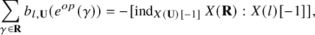$$ \begin{align*}\sum_{\gamma\in\mathbf{R}}b_{l,\mathbf{U}}(e^{op}(\gamma))=-[\operatorname{ind}_{X(\mathbf{U})[-1]}X(\mathbf{R}):X(l)[-1]],\end{align*} $$

which is not zero by Lemma 2.9. Hence, there exists $\gamma \in \mathbf {R}$ such that $b_{l,\mathbf {U}}(e^{op}(\gamma ))\neq 0$ . The last assertion then follows by Remark 2.17.

We have the following geometric interpretation of a certain subcategory of the module category of a surface rigid algebra.

Theorem 4.11. Let $\mathbf {R}$ be a partial tagged triangulation of a punctured marked surface $\mathbf {S}$ , and $\Lambda _{\mathbf {R}}=\operatorname {End}_{\mathcal {C}(\mathbf {S})}X(\mathbf {R})$ the corresponding surface rigid algebra. Then there is a bijection

$$ \begin{align*}M:\operatorname{A}^\times_{\mathbf{R}\operatorname{-st}}\setminus\rho(\mathbf{R})\to\operatorname{ind} \operatorname{\tau-rigid}\operatorname{mod}\Lambda_{\mathbf{R}},\end{align*} $$

where $\operatorname {ind}\operatorname {\tau -rigid}\operatorname {mod}\Lambda _{\mathbf {R}}$ is the set of (isoclasses of) indecomposable $\tau $ -rigid $\Lambda _{\mathbf {R}}$ -modules, such that for any $\gamma _1,\gamma _2\in \operatorname {A}^\times _{\mathbf {R}\operatorname {-st}}\setminus \rho (\mathbf {R})$ , we have

$$ \begin{align*}\operatorname{Int}(\gamma_1,\gamma_2)=\dim_{\mathbf{k}}\operatorname{Hom}_{\Lambda_{\mathbf{R}}}(M(\gamma_1),\tau M(\gamma_2))+\dim_{\mathbf{k}}\operatorname{Hom}_{\Lambda_{\mathbf{R}}}(M(\gamma_2),\tau M(\gamma_1)).\end{align*} $$

Proof. For any $\gamma \in \operatorname {A}^\times _{\mathbf {R}\operatorname {-st}}\setminus \rho (\mathbf {R})$ , define $M(\gamma )=\operatorname {Hom}_{\mathcal {C}(\mathbf {S})}(X(\mathbf {R}),X(\gamma ))$ . Then by Theorem 4.7 and Theorem 2.21, M is a bijection from $\operatorname {A}^\times _{\mathbf {R}\operatorname {-st}}\setminus \rho (\mathbf {R})$ to $\operatorname {ind} \operatorname {\tau -rigid}\operatorname {mod}\Lambda $ .

Let $X_i=X(\gamma _i)$ and $M_i=M(\gamma _i)$ , $i=1,2$ . Then we have

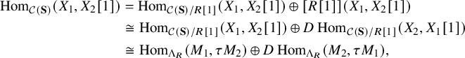$$\begin{align*}\begin{aligned} \operatorname{Hom}_{\mathcal{C}(\mathbf{S})}(X_1,X_2[1])&{}=\operatorname{Hom}_{\mathcal{C}(\mathbf{S})/R[1]}(X_1,X_2[1])\,{\oplus}\,[R[1]](X_1,X_2[1])\\ &\cong\operatorname{Hom}_{\mathcal{C}(\mathbf{S})/R[1]}(X_1,X_2[1])\,{\oplus}\, D\operatorname{Hom}_{\mathcal{C}(\mathbf{S})/R[1]}(X_2,X_1[1])\\ &\cong\operatorname{Hom}_{\Lambda_R}(M_1,\tau M_2)\,{\oplus}\, D\operatorname{Hom}_{\Lambda_R}(M_2,\tau M_1), \end{aligned}\end{align*}$$

where the first isomorphism is due to [18, Lemma 2.3] and the last one is due to Theorem 2.21. By Theorem 3.15, we have $\operatorname {Int}(\gamma _1,\gamma _2)=\dim _{\mathbf {k}}\operatorname {Hom}_{\mathcal {C}(\mathbf {S})}(X_1,X_2[1])$ . Hence, we get the required formula.

4.2 Skew-gentle algebras as surface rigid algebras

In this subsection, we show that skew-gentle algebras are surface rigid algebras. So the geometric model in Theorem 4.11 is a generalization of a weak version of our previous work [33].

Definition 4.12. A triple $(Q,Sp,I)$ of a quiver Q, a subset $Sp\subseteq Q_0$ and a set I of paths of length 2 in Q is called skew-gentle if $(Q^{sp},I^{sp})$ satisfies the following conditions, where $Q^{sp}_0=Q_0, Q^{sp}_1=Q_1\cup \{\epsilon _i\mid i\in Sp\}$ with $\epsilon _i$ a loop at i and $I^{sp}=I\cup \{\epsilon ^2_i\mid i\in Sp\}$ .

• ○ Each vertex in $Q^{sp}_0$ is the start of at most two arrows in $Q_1^{sp}$ , and is the terminal of at most two arrows in $Q_1^{sp}$ ;

• ○ For each arrow $\alpha \in Q^{sp}_1$ , there is at most one arrow $\beta \in Q^{sp}_1$ (resp. $\gamma \in Q^{sp}_1$ ) such that $\alpha \beta \in I^{sp}$ (resp. $\alpha \gamma \notin I^{sp}$ );

• ○ For each arrow $\alpha \in Q^{sp}_1$ , there is at most one arrow $\beta \in Q^{sp}_1$ (resp. $\gamma \in Q^{sp}_1$ ) such that $\beta \alpha \in I^{sp}$ (resp. $\gamma \alpha \notin I^{sp}$ ).

A finite-dimensional algebra $\Lambda $ is said to be skew-gentle if $\Lambda \cong {\mathbf {k}} Q^{sp}/{\langle }I^{sg}{\rangle }$ for some skew-gentle triple $(Q,Sp,I)$ , where ${\langle }I^{sg}{\rangle }$ is the ideal generated by $I^{sg}=I\cup \{\epsilon ^2_i-\epsilon _i\mid i\in Sp\}$ .

A partial ideal triangulation of $\mathbf {S}$ is called admissible if each puncture is contained in a self-folded triangle.

Definition 4.13 [9, Definition 2.1],[33, Definition 1.8]

Let $\mathbf {R}$ be an admissible partial ideal triangulation of $\mathbf {S}$ . Denote by $\mathbf {R}_0$ the subset of $\mathbf {R}$ such that $\mathbf {R}\setminus \mathbf {R}_0$ consists of the folded sides of self-folded triangles of $\mathbf {R}$ , and by $\mathbf {R}_1$ the subset of $\mathbf {R}_0$ consisting of the non-folded sides of self-folded triangles of $\mathbf {R}$ . The tiling algebra of $\mathbf {R}$ is defined to be $\Lambda ^t_{\mathbf {R}}={\mathbf {k}} Q_{\mathbf {R}}/{\langle }I^t_{\mathbf {R}}{\rangle }$ , where the quiver $Q_{\mathbf {R}}=((Q_{\mathbf {R}})_0,(Q_{\mathbf {R}})_1,s,t)$ and the relation set $I^t_{\mathbf {R}}$ are given by the following.

• ○ The vertices in $(Q_{\mathbf {R}})_0$ are (indexed by) the arcs in $\mathbf {R}_0$ .

• ○ There is an arrow $\alpha \in (Q_{\mathbf {R}})_1$ from i to j whenever the corresponding arcs i and j share an endpoint $p_{\alpha }\in \mathbf {M}$ such that j follows i anticlockwise immediately in $\mathbf {R}_0$ . Note that by this construction, each vertex in $(Q_{\mathbf {R}})_0$ admits at most one loop.

• ○ The relation set $I^t_{\mathbf {R}}=I^t_{\mathbf {R},1}\cup I^t_{\mathbf {R},2}$ , where

  • – $I^t_{\mathbf {R},1}$ consists of squares of loops in $(Q_{\mathbf {R}})_1$ , and

  • – $I^t_{\mathbf {R},2}$ consisting of all $\alpha \beta $ if $p_{\beta }\neq p_{\alpha }$ , or the endpoints of the curve (corresponding to) $t(\beta )=s(\alpha )$ coincide and we are in one of the situations in Figure 9.

    

    Figure 9 Relations in $I^t_{\mathbf {R},2}$ , the case $p_\beta =p_\alpha $ and $s(\alpha )=t(\beta )$ is a loop.

Let $I^{s\text {-}t}_{\mathbf {R}}$ be the subset obtained from $I^t_{\mathbf {R}}$ by replacing $\epsilon ^2$ with $\epsilon ^2-\epsilon $ for each loop $\epsilon $ at a vertex in $\mathbf {R}_1$ . The skew-tiling algebra of $\mathbf {R}$ is defined to be $\Lambda ^{s\text {-}t}_{\mathbf {R}}={\mathbf {k}} Q_{\mathbf {R}}/{\langle }I^{s\text {-}t}_{\mathbf {R}}{\rangle }$ .

By definition, skew-tiling algebras are obtained from tiling algebras by specializing nilpotent loops at vertices in $\mathbf {R}_1$ to be idempotents.

Remark 4.14. In the original definition of tiling algebras introduced in [9], there are no punctures on the surface. However, after replacing each puncture by a boundary component with a marked point, and replacing each self-folded triangle of $\mathbf {R}$ by a monogon with the corresponding new boundary component in its interior, our definition coincides with the original one.

Theorem 4.15 [9, Theorem 1] and [33, Corollary 1.12]

A finite-dimensional algebra is a (skew-)gentle algebra if and only if it is a (skew-)tiling algebra.

In the following, we show that the skew-gentle algebras form a special class of surface rigid algebras.

Theorem 4.16. Let $\mathbf {R}$ be an admissible partial ideal triangulation of $\mathbf {S}$ and $\Lambda _{\mathbf {R}}=\operatorname {End}_{\mathcal {C}(\mathbf {S})}(X(\mathbf {R}))$ the corresponding surface rigid algebra. Then there is an algebra isomorphism

$$\begin{align*}\Lambda_{\mathbf{R}}\cong\Lambda^{s\text{-}t}_{\mathbf{R}}.\end{align*}$$

In particular, skew-gentle algebras are surface rigid algebras.

Proof. Let $\mathbf {T}$ be an admissible triangulation containing $\mathbf {R}$ . By [2, Theorem 3.5], there is an algebra isomorphism

$$\begin{align*}\psi:\operatorname{End}_{\mathcal{C}(\mathbf{S})}X(\mathbf{T})\cong\Lambda^{\mathbf{T}}\end{align*}$$

sending the identity $\operatorname {id}_{X(\gamma )}$ of $X(\gamma )$ to the idempotent $e^\gamma $ of $\Lambda ^{\mathbf {T}}$ corresponding to $\gamma \in Q_0^{\mathbf {T}}$ , for any $\gamma \in \mathbf {T}$ . Let $e^{\mathbf {R}}=\sum _{\gamma \in \mathbf {R}}e^\gamma \in \Lambda ^{\mathbf {T}}$ and $e_{\mathbf {R}}=\sum _{\gamma \in \mathbf {R}_0}e_\gamma \in \Lambda ^{s\text {-}t}_{\mathbf {T}}$ , where $e_\gamma $ is the idempotent of $\Lambda ^{s\text {-}t}_{\mathbf {T}}$ corresponding to $\gamma \in \mathbf {R}_0$ . So we have

$$\begin{align*}\Lambda_{\mathbf{R}}=\operatorname{End}_{\mathcal{C}(\mathbf{S})}X(\mathbf{R})=\operatorname{id}_{R}\operatorname{End}_{\mathcal{C}(\mathbf{S})}X(\mathbf{T})\operatorname{id}_{R}\cong e^{\mathbf{R}}\Lambda^{\mathbf{T}} e^{\mathbf{R}}\cong e_{\mathbf{R}}\Lambda^{s\text{-}t}_{\mathbf{T}} e_{\mathbf{R}},\end{align*}$$

where the first isomorphism is induced by $\psi $ , and the last isomorphism is due to [49, Proposition 4.4].

Let $\mathbf {S}^t$ be the unpunctured marked surface obtained from $\mathbf {S}$ by replacing each puncture by a boundary component with one marked point. By Remark 4.14, $\Lambda ^t_{\mathbf {T}}$ and $\Lambda ^t_{\mathbf {R}}$ are exactly tiling algebras defined in [9] on $\mathbf {S}^t$ . So we have $e_{\mathbf {R}}\Lambda ^t_{\mathbf {T}} e_{\mathbf {R}}\cong \Lambda ^t_{\mathbf {R}}$ by [9, Theorem 2.8]. Denote by $\mathbf {T}_1$ the subset of $\mathbf {T}$ consisting of all non-folded sides of self-folded triangles. Since $\mathbf {R}$ is admissible, we have $\mathbf {R}_1=\mathbf {T}_1$ . So $\Lambda ^{s\text {-}t}_{\mathbf {T}}$ and $\Lambda ^{s\text {-}t}_{\mathbf {R}}$ are obtained from $\Lambda ^t_{\mathbf {T}}$ and $\Lambda ^t_{\mathbf {R}}$ , respectively, by specializing the same set of nilpotent loops to be idempotents. Hence, $e_{\mathbf {R}}\Lambda ^{s\text {-}t}_{\mathbf {T}} e_{\mathbf {R}}\cong \Lambda ^{s\text {-}t}_{\mathbf {R}}$ , which implies the isomorphism $\Lambda _{\mathbf {R}}\cong \Lambda ^{s\text {-}t}_{\mathbf {R}}$ .

The last assertion then follows from Theorem 4.15.

5 Connectedness of exchange graphs

Throughout this section, let $\mathbf {R}$ be a partial tagged triangulation of a punctured marked surface $\mathbf {S}$ and $\Lambda _{\mathbf {R}}=\operatorname {End}_{\mathcal {C}(\mathbf {S})}X(\mathbf {R})$ the corresponding surface rigid algebra.

5.1 Flips of dissections

Recall from Definition 3.3 that $\operatorname {A}^\times (\mathbf {S})$ denotes the set of tagged arcs on $\mathbf {S}$ . For any tagged arc $\eta \in \operatorname {A}^\times (\mathbf {S})$ , let

$$ \begin{align*}\operatorname{A}^\times(\mathbf{S})_{\{\eta\}}=\{\gamma\in\operatorname{A}^\times(\mathbf{S})\setminus\{\eta\}\mid \operatorname{Int}(\gamma,\eta)=0\},\end{align*} $$

and let $\mathbf {S}/\{\eta \}$ be the punctured marked surface obtained from $\mathbf {S}$ by cutting along $\eta $ (cf. [49, Section 5.2]). Then there is a natural bijection

$$ \begin{align*}F_{\{\eta\}}:\operatorname{A}^\times(\mathbf{S})_{\{\eta\}}\to\operatorname{A}^\times(\mathbf{S}/{\{\eta\}}),\end{align*} $$

sending $\gamma $ to the tagged arc on $\mathbf {S}/\{\eta \}$ obtained from $\gamma $ by forgetting the taggings at each puncture which is an endpoint of $\eta $ (and hence becomes a marked point on the boundary of $\mathbf {S}/{\{\eta \}}$ ), unless $\gamma $ is homotopic to $\eta $ , where $F_{\{\eta \}}(\gamma )$ is the tagged arc shown in Figure 10. Note that for any $\gamma _1,\gamma _2\in \operatorname {A}^\times (\mathbf {S})_{\{\eta \}}$ , we have $\operatorname {Int}(\gamma _1,\gamma _2)=0$ if and only if $\operatorname {Int}(F_{\{\eta \}}(\gamma _1),F_{\{\eta \}}(\gamma _2))=0$ . Therefore, $F_{\{\eta \}}$ induces a bijection from the set of partial tagged triangulations of $\mathbf {S}$ containing $\eta $ to the set of partial tagged triangulations of $\mathbf {S}/\{\eta \}$ .

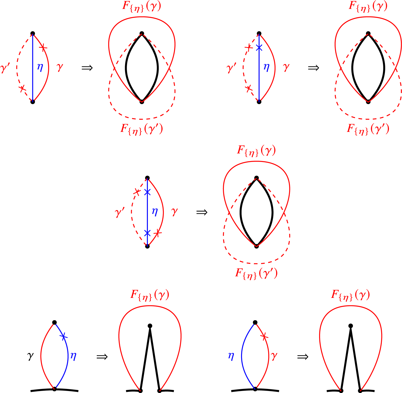
Figure 10 The bijection $F_{\{\eta \}}$ .

For any partial tagged triangulation $\mathbf {N}$ of $\mathbf {S}$ , set

$$ \begin{align*}\operatorname{A}^\times(\mathbf{S})_{\mathbf{N}}=\{\gamma\in\operatorname{A}^\times(\mathbf{S})\setminus\mathbf{N}\mid \operatorname{Int}(\gamma,\eta)=0,\text{ for any} \eta\in\mathbf{N}\}.\end{align*} $$

Assume that we have defined a punctured marked surface $\mathbf {S}/{\mathbf {N}^{\prime }}$ and a bijection $F_{\mathbf {N}^{\prime }}:\operatorname {A}^\times (\mathbf {S})_{\mathbf {N}^{\prime }}\to \operatorname {A}^\times (\mathbf {S}/\mathbf {N}^{\prime })$ for some $\mathbf {N}^{\prime }\subset \mathbf {N}$ with $\mathbf {N}=\mathbf {N}^{\prime }\cup \{\eta \}$ . Then $F_{\mathbf {N}^{\prime }}$ restricts to a bijection $F_{\mathbf {N}^{\prime }}|_{\operatorname {A}^\times (\mathbf {S})_{\mathbf {N}}}:\operatorname {A}^\times (\mathbf {S})_{\mathbf {N}}\to \operatorname {A}^\times (\mathbf {S}/\mathbf {N}^{\prime })_{F_{\mathbf {N}^{\prime }}(\eta )}$ . So we can define inductively the punctured marked surface

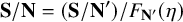$$ \begin{align*}\mathbf{S}/\mathbf{N}=(\mathbf{S}/\mathbf{N}^{\prime})/F_{\mathbf{N}^{\prime}}(\eta)\end{align*} $$

and the bijection

$$ \begin{align*}F_{\mathbf{N}}=F_{F_{\mathbf{N}^{\prime}}(\eta)}\circ F_{\mathbf{N}^{\prime}}|_{\operatorname{A}^\times(\mathbf{S})_{\mathbf{N}}}:\operatorname{A}^\times(\mathbf{S})_{\mathbf{N}}\to\operatorname{A}^\times(\mathbf{S}/\mathbf{N}).\end{align*} $$

Recall from Theorem 2.23 that $\mathcal {C}(\mathbf {S})_{X(\mathbf {N})}={}^\bot X(\mathbf {N})[1]/{\langle }\operatorname {add} X(\mathbf {N}){\rangle }$ is a triangulated category.

Lemma 5.1. Let $\mathbf {N}$ be a partial tagged triangulation of $\mathbf {S}$ . Then there is a triangle equivalence

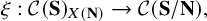(5.1) $$ \begin{align} \xi:\mathcal{C}(\mathbf{S})_{X(\mathbf{N})}\to\mathcal{C}(\mathbf{S}/\mathbf{N}), \end{align} $$

such that

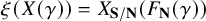(5.2) $$ \begin{align} \xi(X(\gamma))=X_{\mathbf{S}/\mathbf{N}}(F_{\mathbf{N}}(\gamma)) \end{align} $$

holds for any $\gamma \in \operatorname {A}^\times (\mathbf {S})_{\mathbf {N}}$ , where $X_{\mathbf {S}/\mathbf {N}}$ is the bijection in Theorem 3.15 for $\mathbf {S}/\mathbf {N}$ .

Proof. Let $\mathbf {T}$ be a tagged triangulation containing $\mathbf {N}$ . Then $F_{\mathbf {N}}(\mathbf {T}\setminus \mathbf {N})$ is a tagged triangulation of $\mathbf {S}/\mathbf {N}$ and the corresponding quiver with potential $(Q^{F_{\mathbf {N}}(\mathbf {T}\setminus \mathbf {N})},W^{F_{\mathbf {N}}(\mathbf {T}\setminus \mathbf {N})})$ can be obtained from the quiver with potential $(Q^{\mathbf {T}},W^{\mathbf {T}})$ by deleting the vertices corresponding to the tagged arcs in $\mathbf {N}$ and the incident arrows. Then by [36, Theorem 7.4], the canonical projection $\pi :\Lambda ^{\mathbf {T}}\to \Lambda ^{F_{\mathbf {N}}(\mathbf {T}\setminus \mathbf {N})}$ induces the triangle equivalence (5.1) such that (5.2) holds for any $\gamma \in \mathbf {T}\setminus \mathbf {N}$ . Then by Theorem 3.15, (5.2) holds for any $\gamma \in \operatorname {A}^\times (\mathbf {S})_{\mathbf {N}}$ .

Recall from Construction 3.8 that for any partial tagged triangulation $\mathbf {N}$ , there is an associated partial ideal triangulation $\mathbf {N}^\circ $ . For any $l\in \mathbf {N}$ , denote by $l^{\circ _{\mathbf {N}}}$ the arc in $\mathbf {N}^\circ $ corresponding to l, which is sometimes simply denoted by $l^\circ $ when there is no confusion arising.

Remark 5.2. Let $\mathbf {N}$ be a partial tagged triangulation of $\mathbf {S}$ . By the construction, $\mathbf {S}/\mathbf {N}$ is obtained from $\mathbf {S}$ by cutting along arcs in $\mathbf {N}^\circ $ .

Definition 5.3. Let $\mathbf {N}$ be a partial tagged triangulation of $\mathbf {S}$ . The tagged rotation with respect to $\mathbf {N}$ is defined to be the bijection

$$ \begin{align*}\rho_{\mathbf{N}}=F_{\mathbf{N}}^{-1}\circ\rho_{\mathbf{S}/\mathbf{N}}\circ F_{\mathbf{N}}:\operatorname{A}^\times(\mathbf{S})_{\mathbf{N}}\to\operatorname{A}^\times(\mathbf{S})_{\mathbf{N}},\end{align*} $$

where $\rho _{\mathbf {S}/\mathbf {N}}$ is the tagged rotation on $\mathbf {S}/\mathbf {N}$ .

To better understand the tagged rotation with respect to a partial tagged triangulation, we introduce the following notion of flip of a partial ideal triangulation.

Definition 5.4. Let $\mathbf {V}$ be a partial ideal triangulation of $\mathbf {S}$ and $l^\circ \in \mathbf {V}$ not the folded side of a self-folded triangle of $\mathbf {V}$ . Recall that B is the set of boundary segments. We denote

• ○ $l^\circ _s$ (resp. $l^\circ _t$ ) the arc in $\mathbf {V}\cup B$ the first arc in $(\mathbf {V}\setminus \{l^\circ \})\cup B$ next to $l^\circ $ around $l^\circ (0)=l^\circ _s(0)$ (resp. $l^\circ (1)=l^\circ _t(1)$ ) in the clockwise order, and

• ○ $(l^\circ )^s$ (resp. $(l^\circ )^t$ ) the first arc in $(\mathbf {V}\setminus \{l^\circ \})\cup B$ next to $l^\circ $ around $l^\circ (0)=(l^\circ )^s(0)$ (resp. $l^\circ (1)=(l^\circ )^t(1)$ ) in the anticlockwise order.

See Figures 17 and 18 for these notations. We remark that some of $l^\circ _s,l^\circ _t,(l^\circ )^s,(l^\circ )^t$ may not exist.

The negative (resp. positive) flip $f^-_{\mathbf {V}}(l^\circ )$ (resp. $f^+_{\mathbf {V}}(l^\circ )$ ) of $l^\circ $ with respect to $\mathbf {V}$ is defined to be the arc obtained from $l^\circ $ by moving $l^\circ (0)$ along $l^\circ _s$ (resp. $(l^\circ )^s$ ), if exists, to $l^\circ _s(1)$ (resp. $(l^\circ )^s(1)$ ) and moving $l^\circ (1)$ along $l^\circ _t$ (resp. $(l^\circ )^t$ ), if exists, to $l^\circ _t(0)$ (resp. $(l^\circ )^t(0)$ ). The positive flip $f^+_{l^\circ }(\mathbf {V})$ and the negative flip $f^-_{l^\circ }(\mathbf {V})$ of $\mathbf {V}$ at $l^\circ $ are defined, respectively, to be

$$ \begin{align*}f^+_{l^\circ}(\mathbf{V})=(\mathbf{V}\setminus\{l^\circ\})\cup\{f^+_{\mathbf{V}}(l^\circ)\},\ f^-_{l^\circ}(\mathbf{V})=(\mathbf{V}\setminus\{l^\circ\})\cup\{f^-_{\mathbf{V}}(l^\circ)\}.\end{align*} $$

We also denote by $\theta _s$ (resp. $\theta ^s$ , $\theta _t$ and $\theta ^t$ ) the angle between a segment of $l^\circ $ near $l^\circ (0)$ (resp. $l^\circ (0)$ , $l^\circ (1)$ and $l^\circ (1)$ ) and a segment of $l^\circ _s$ (resp. $(l^\circ )^s$ , $l^\circ _t$ and $(l^\circ )^t$ ) near $l^\circ _s(0)$ (resp. $(l^\circ )^s(0)$ , $l^\circ _t(1)$ and $(l^\circ )^t(1)$ ).

Lemma 5.5. Let $\mathbf {U}=\mathbf {N}\cup \{l\}$ be a partial tagged triangulation of $\mathbf {S}$ such that $l^\circ $ is not the folded side of a self-folded triangle of $\mathbf {U}^\circ $ . Then $(\mathbf {N}\cup \{\rho ^{-1}_{\mathbf {N}}(l)\})^\circ =f^-_{l^\circ }(\mathbf {U}^\circ )$ and $(\mathbf {N}\cup \{\rho _{\mathbf {N}}(l)\})^\circ =f^+_{l^\circ }(\mathbf {U}^\circ )$ .

Proof. We only prove the first equality while the second can be proved similarly. Since $l^\circ $ is not the folded side of a self-folded triangle of $\mathbf {U}^\circ $ , we have $\mathbf {U}^\circ =\mathbf {N}^\circ \cup \{l^\circ \}$ and that $F_{\mathbf {N}}(l)$ is homotopic to $l^\circ $ . By Remark 5.2, $\mathbf {S}/\mathbf {N}$ is obtained from $\mathbf {S}$ by cutting the surface along arcs in $\mathbf {N}^\circ $ . Then $l^\circ _s$ and $l^\circ _t$ (if exist) are the boundary segments of $\mathbf {S}/\mathbf {N}$ next to $F_{\mathbf {N}}(l)$ around $l^\circ (0)$ and $l^\circ (1)$ , respectively, in the clockwise order. Hence, by definition, $\rho ^{-1}_{\mathbf {S}/\mathbf {N}}(F_{\mathbf {N}}(l))$ is homotopic to $f^-_{\mathbf {U}^\circ }(l^\circ )$ .

Denote $\mathbf {U}^{\prime }=\mathbf {N}\cup \{\rho ^{-1}_{\mathbf {N}}(l)\}$ . If $\rho ^{-1}_{\mathbf {N}}(l)$ is not the folded side of a self-folded triangle of ${\mathbf {U}^{\prime }}^\circ $ , then

$$ \begin{align*}{\mathbf{U}^{\prime}}^\circ=\mathbf{N}^\circ\cup\{\rho^{-1}_{\mathbf{N}}(l)^{\circ_{\mathbf{U}^{\prime}}}\}=\mathbf{N}^\circ\cup\{F_{\mathbf{N}}(\rho^{-1}_{\mathbf{N}}(l))\}=\mathbf{N}^\circ\cup \{f^-_{\mathbf{U}^\circ}(l^\circ)\}=f^-_{l^\circ}(\mathbf{U}^\circ).\end{align*} $$

If $\rho ^{-1}_{\mathbf {N}}(l)$ is the folded side of a self-folded triangle $\Delta $ of $\mathbf {U}^{\prime \circ }$ , then there is $h\in \mathbf {N}$ such that $h^{\circ _{\mathbf {U}^{\prime }}}$ is the non-folded side of $\Delta $ . So $h^{\circ _{\mathbf {U}^{\prime }}}$ is homotopic to $f^-_{\mathbf {U}^\circ }(l^\circ )$ and $\rho ^{-1}_{\mathbf {N}}(l)^{\circ _{\mathbf {U}^{\prime }}}$ is homotopic to $h^{\circ _{\mathbf {N}}}=h^{\circ _{\mathbf {U}}}$ . Thus, we also have ${\mathbf {U}^{\prime }}^\circ =f^-_{l^\circ }(\mathbf {U}^\circ )$ .

By Lemma 4.10, for any l in an $\mathbf {R}$ -dissection $\mathbf {U}$ , either there exists $\gamma \in \mathbf {R}$ such that or there exists $\gamma \in \mathbf {R}$ such that $b_{l,\mathbf {U}}(e^{op}(\gamma ))<0$ , but not both. This ensures the well-definedness of the following notion of flip of dissections.

Definition 5.6. Let $\mathbf {U}$ be an $\mathbf {R}$ -dissection. For any $l\in \mathbf {U}$ , the flip $f^{\mathbf {R}}_l(\mathbf {U})$ of $\mathbf {U}$ at l is defined to be

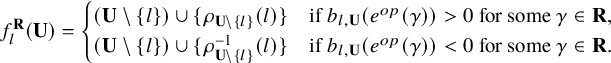
We denote by $f^{\mathbf {R}}_{\mathbf {U}}(l)$ the tagged arc in $f_l^{\mathbf {R}}(\mathbf {U})$ , but not in $\mathbf {U}$ .

We will simply denote $f_{\mathbf {U}}(l)=f_{\mathbf {U}}^{\mathbf {R}}(l)$ and $f_{l}(\mathbf {U})=f_{l}^{\mathbf {R}}(\mathbf {U})$ when there is no confusion arising. By Lemma 5.5, for any $l\in \mathbf {U}$ such that $l^\circ $ is not the folded side of a self-folded triangle of $\mathbf {U}^\circ $ , we have

(5.3)

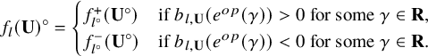
Remark 5.7. In the case that $\mathbf {R}$ is a tagged triangulation, the $\mathbf {R}$ -dissections are exactly the tagged triangulations of $\mathbf {S}$ , and the flip in Definition 5.6 coincides with the flip of tagged triangulations introduced in [25].

Proposition 5.8. For any $\mathbf {R}$ -dissection $\mathbf {U}$ and any $l\in \mathbf {U}$ , we have that $f_l(\mathbf {U})$ is the unique $\mathbf {R}$ -dissection such that $\mathbf {U}\setminus f_l(\mathbf {U})=\{l\}$ . Moreover, under the bijection (4.1) in Theorem 4.7, the flip of $\mathbf {R}$ -dissections is compatible with the mutation of maximal rigid objects with respect to $X(\mathbf {R})\ast X(\mathbf {R})[1]$ .

Proof. Let $\mathbf {N}=\mathbf {U}\setminus \{l\}$ . It suffices to show $X(f_l(\mathbf {U}))$ is the unique (up to isomorphism) basic maximal rigid object with respect to $X(\mathbf {R})\ast X(\mathbf {R})[1]$ such that $X(f_l(\mathbf {U}))$ contains $X(\mathbf {N})$ as a direct summand and is not isomorphic to $X(\mathbf {U})$ . By Corollary 2.16 and Remark 2.17, this is equivalent to showing

Then by (3.3), it suffices to show

$$ \begin{align*}X((\mathbf{U}\setminus\{l\})\cup\{\rho_{\mathbf{N}}(l)\})=\mu_{X(l)}^-(X(\mathbf{U}))\end{align*} $$

and

$$ \begin{align*}X((\mathbf{U}\setminus\{l\})\cup\{\rho^{-1}_{\mathbf{N}}(l)\})=\mu_{X(l)}^+(X(\mathbf{U})).\end{align*} $$

By Remark 2.24, this is equivalent to showing that

$$ \begin{align*}X(\rho_{\mathbf{N}}(l))=X(l){\langle}1{\rangle}_{X(\mathbf{N})}\text{ and }X(\rho^{-1}_{\mathbf{N}}(l))=X(l){\langle}-1{\rangle}_{X(\mathbf{N})},\end{align*} $$

where ${\langle }1{\rangle }_{X(\mathbf {N})}$ and ${\langle }-1{\rangle }_{X(\mathbf {N})}$ are the suspension functor of $\mathcal {C}(\mathbf {S})_{\mathbf {N}}$ and its inverse, respectively (see Theorem 2.23).

Using (5.2), we have

$$ \begin{align*}\xi(X(\rho_{\mathbf{N}}(l)))=X_{\mathbf{S}/\mathbf{N}}(\rho_{\mathbf{S}/\mathbf{N}}(F_{\mathbf{N}}(l)))=X_{\mathbf{S}/\mathbf{N}}(F_{\mathbf{N}}(l))[1]=\xi(X(l){\langle}1{\rangle}_{X(\mathbf{N})}).\end{align*} $$

Hence, $X(\rho _{\mathbf {N}}(l))=X(l)\langle 1\rangle _{X(\mathbf {N})}$ . Similarly, we have $X(\rho ^{-1}_{\mathbf {N}}(l))=X(l)\langle -1\rangle _{X(\mathbf {N})}$ .

Definition 5.9. The exchange graph $\operatorname {EG}^\times (\mathbf {R})$ of $\mathbf {R}$ -dissections has $\mathbf {R}$ -dissections as vertices and has flips as edges.

Lemma 5.10. There is an isomorphism of graphs $\operatorname {EG}^\times (\mathbf {R})\cong \operatorname {EG}(\operatorname {s\tau -tilt} \Lambda _{\mathbf {R}})$ .

Proof. By Theorem 2.21 and Theorem 4.7, there is a bijection between support $\tau $ -tilting A-modules and $\mathbf {R}$ -dissections, such that, by Theorem 2.22 and Proposition 5.8, the mutations of support $\tau $ -tilting modules are compatible with the flips of $\mathbf {R}$ -dissections. Thus, we can get the required isomorphism.

Example 5.11. Let $\mathbf {S}$ be a punctured marked surface with genus zero, two boundary components and one puncture as shown in the left picture of Figure 11, where a partial ideal triangulation $\mathbf {R}$ consisting of the red arcs $1,2$ and $3$ is given. Then, by Theorem 4.16, the corresponding surface rigid algebra $\Lambda _{\mathbf {R}}$ is isomorphic to the skew-gentle algebra ${\mathbf {k}} Q_{\mathbf {R}}/\langle I_{\mathbf {R}}^{s\text {-}t}\rangle $ , where $Q_{\mathbf {R}}$ is shown in the right picture of Figure 11 and the relation set $I^{s\text {-}t}_{\mathbf {R}}=\{ba,ab,\epsilon ^2-\epsilon \}$ .

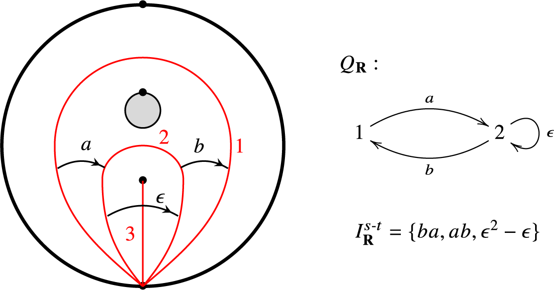
Figure 11 An example of a partial ideal triangulation of a marked surface with the associated surface rigid algebra.

The algebra ${\mathbf {k}} Q_{\mathbf {R}}/I^{s\text {-}t}_{\mathbf {R}}$ is Morita equivalent to $\Lambda ={\mathbf {k}} Q/\langle I\rangle $ , where

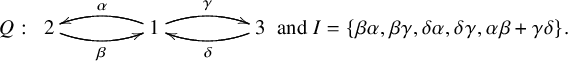
For any vertex i of Q, let $S_i$ , $P_i$ and $I_i$ be the corresponding simple, projective module and injective module, respectively. Let $M,N$ be the following two representations of Q bounded by I:

Then the Auslander-Reiten quiver of $\Lambda $ is as follows:

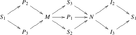
The exchange graph of support $\tau $ -tilting $\Lambda $ -modules is shown in Figure 12, and the corresponding isomorphic exchange graph of $\mathbf {R}$ -dissections is shown in Figure 13.

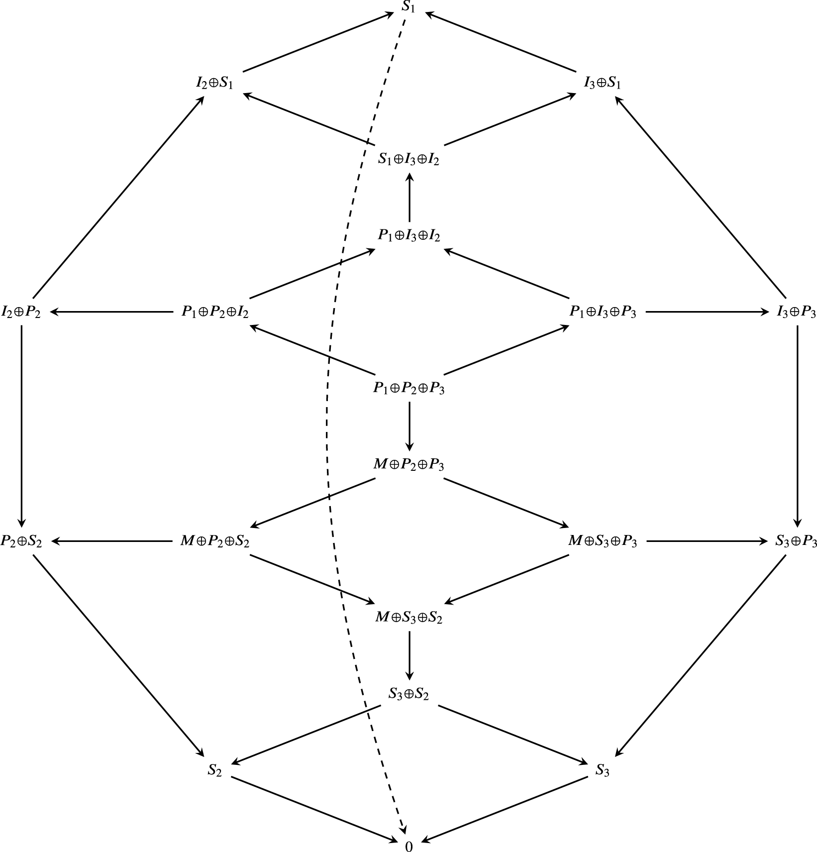
Figure 12 An exchange graph of support $\tau $ -tilting modules.

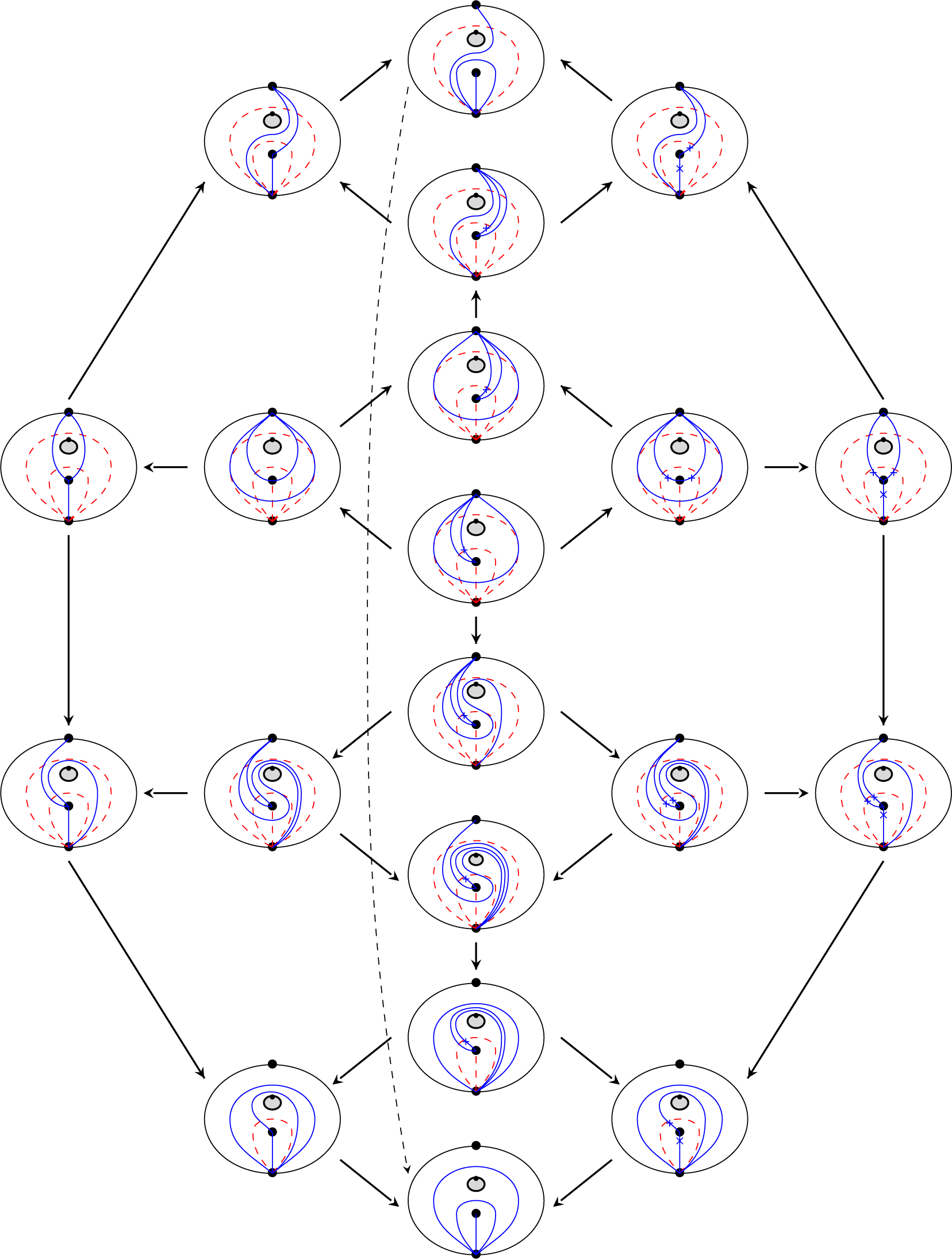
Figure 13 An exchange graph of dissections.

A subset $\mathbf {R}_1$ of $\mathbf {R}$ is said to be connected if there is no decomposition $\mathbf {R}_1=\mathbf {R}^{\prime }\cup \mathbf {R}^{\prime \prime }$ such that any arc in $\mathbf {R}^{\prime }$ and any arc in $\mathbf {R}^{\prime \prime }$ have no endpoints in common. A connected component of $\mathbf {R}$ is a maximal connected subset of $\mathbf {R}$ .

Definition 5.12. We call $\mathbf {R}$ is connected to the boundary if each connected component of $\mathbf {R}$ contains at least one arc incident to a marked point in $\mathbf {M}$ .

For any $\eta \in \mathbf {R}$ , we denote by $\mathbf {R}/\{\eta \}$ the partial tagged triangulation $F_{\{\eta \}}(\mathbf {R}\setminus \{\eta \})$ of $\mathbf {S}/\{\eta \}$ .

Lemma 5.13. If $\mathbf {R}$ is connected to the boundary, then so does $\mathbf {R}/\{\eta \}$ .

Proof. Let $\mathbf {R}=\mathbf {R}^{\prime }\cup \mathbf {R}^{\prime \prime }$ with $\mathbf {R}^{\prime }$ the connected component of $\mathbf {R}$ containing $\eta $ . Let $\mathbf {R}^{\prime }\setminus \{\eta \}=\mathbf {R}_1\cup \cdots \cup \mathbf {R}_s$ with $\mathbf {R}_i,1\leq i\leq s$ , connected components of $\mathbf {R}^{\prime }\setminus \{\eta \}$ . Since $\mathbf {R}^{\prime }$ is connected, for each $1\leq i\leq s$ , there exists $\gamma _i\in \mathbf {R}_i$ having a common endpoint with $\eta $ . So $F_{\{\eta \}}(\gamma _i)$ has a marked point as an endpoint. Hence, $F_{\{\eta \}}(\mathbf {R}\setminus \{\eta \})= F_{\{\eta \}}(\mathbf {R}_1)\cup \cdots \cup F_{\{\eta \}}(\mathbf {R}_s)\cup F_{\{\eta \}}(\mathbf {R}^{\prime \prime })$ is also connected to the boundary.

Denote by $D(\mathbf {R})_{\{\eta \}}$ the subset of $D(\mathbf {R})$ consisting of all $\mathbf {R}$ -dissections containing $\eta $ , and $D(\mathbf {R}/\{\eta \})$ the set of $\mathbf {R}/\{\eta \}$ -dissections on $\mathbf {S}/\{\eta \}$ .

Lemma 5.14. There is a bijection

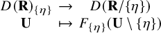$$ \begin{align*}\begin{array}{ccc} D(\mathbf{R})_{\{\eta\}} & \to & D(\mathbf{R}/\{\eta\}) \\ \mathbf{U} & \mapsto & F_{\{\eta\}}(\mathbf{U}\setminus\{\eta\}) \end{array}\end{align*} $$

such that flips on both sides are compatible.

Proof. The bijection (4.1) in Theorem 4.7 restricts a bijection

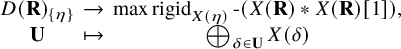$$ \begin{align*}\begin{array}{ccc} D(\mathbf{R})_{\{\eta\}} & \to & \operatorname{max}\operatorname{rigid}_{X(\eta)}\operatorname{-}(X(\mathbf{R})\ast X(\mathbf{R})[1]), \\ \mathbf{U} & \mapsto & \bigoplus_{\delta\in\mathbf{U}}X(\delta) \end{array}\end{align*} $$

such that, by Proposition 5.8, the flip on the left side is compatible with the mutation on the right side. By Proposition 2.25, there is a bijection

$$ \begin{align*}\begin{array}{ccc} \operatorname{max}\operatorname{rigid}_{X(\eta)}\operatorname{-}(X(\mathbf{R})\ast X(\mathbf{R})[1]) & \to & \operatorname{max}\operatorname{rigid-}(X(\mathbf{R})\ast_{\mathcal{C}(\mathbf{S})_{X(\eta)}} X(\mathbf{R}){\langle}1{\rangle}), \\ \mathbf{U} & \mapsto & X(\mathbf{U}\setminus\{\eta\}) \end{array}\end{align*} $$

such that the mutations on both sides are compatible. The triangle equivalence (5.1) for $\mathbf {N}=\{\eta \}$ gives rise to a bijection

$$ \begin{align*}\begin{array}{ccc} \operatorname{max}\operatorname{rigid-}(X(\mathbf{R})\ast_{\mathcal{C}(\mathbf{S})_{X(\eta)}} X(\mathbf{R}){\langle}1{\rangle}) & \to & \operatorname{max}\operatorname{rigid-}(R^{\prime}\ast_{\mathcal{C}(\mathbf{S}/\{\eta\})} R^{\prime}[1]), \\ X(\mathbf{U}\setminus\{\eta\}) & \mapsto & X_{\mathbf{S}/\{\eta\}}(F_{\{\eta\}}(\mathbf{U}\setminus\{\eta\})) \end{array}\end{align*} $$

such that the mutations on both sides are compatible, where $R^{\prime }=X_{\mathbf {S}/\{\eta \}}(\mathbf {R}/\{\eta \})$ . Combining the above three bijections, we get the required one.

The following lemma, which is crucial in the proof of the main result, will be proved in the next subsection.

Lemma 5.15. Let $\mathbf {R}$ be a partial tagged triangulation on $\mathbf {S}$ connected to the boundary. Then for any $\mathbf {R}$ -dissection $\mathbf {U}$ , there exists a sequence of flips $f_{l_1},\cdots ,f_{l_k}$ such that $\mathbf {R}\cap f_{l_k}\circ \cdots \circ f_{l_1}(\mathbf {U})\neq \emptyset $ .

The main result in this section is the following connectedness of the graph of $\mathbf {R}$ -dissections.

Theorem 5.16. Let $\mathbf {R}$ be a partial tagged triangulation on $\mathbf {S}$ connected to the boundary. Then the exchange graph $\operatorname {EG}^\times (\mathbf {R})$ is connected.

Proof. We call two $\mathbf {R}$ -dissections $\mathbf {U}$ and $\mathbf {U}^{\prime }$ flip-connected to each other if one can be obtained from the other by a sequence of flips. To show that $\operatorname {EG}^\times (\mathbf {R})$ is connected, it is enough to show the assertion that any $\mathbf {R}$ -dissection $\mathbf {U}$ is flip-connected to $\mathbf {R}$ . We use the induction on $|\mathbf {R}|$ . When $|\mathbf {R}|=1$ , the assertions follows directly from Lemma 5.15. Suppose the assertion is true when $|\mathbf {R}|\leq n-1$ for some , and consider the case when $|\mathbf {R}|=n$ . By Lemma 5.15, there exists some $\eta \in \mathbf {R}$ and an $\mathbf {R}$ -dissection $\mathbf {U}^{\prime }$ such that $\eta \in \mathbf {R}\cap \mathbf {U}^{\prime }$ and $\mathbf {U}^{\prime }$ is flip-connected to $\mathbf {U}$ . By Lemma 5.14, $F_{\{\eta \}}(\mathbf {U}^{\prime }\setminus \{\eta \})$ is an $\mathbf {R}/\{\eta \}$ -dissection. By Lemma 5.13, $\mathbf {R}/\{\eta \}$ is a partial tagged triangulation of $\mathbf {S}/\{\eta \}$ connected to the boundary. Since $|\mathbf {R}/\{\eta \}|=n-1$ , using the induction hypothesis, $F_{\{\eta \}}(\mathbf {U}^{\prime }\setminus \{\eta \})$ is flip-connected to $\mathbf {R}/\{\eta \}$ . Hence, by Lemma 5.14 again, $\mathbf {U}^{\prime }$ is flip-connected to $\mathbf {R}$ . So $\mathbf {U}$ is flip-connected to $\mathbf {R}$ .

Remark 5.17. If $\mathbf {R}$ is a tagged triangulation, it is automatically connected to the boundary. Hence, Theorem 5.16 generalizes [25, Proposition 7.10].

We have the following important consequence.

Corollary 5.18. The exchange graph $\operatorname {EG}(\operatorname {s\tau -tilt} A)$ of support $\tau $ -tilting modules over any surface rigid algebra A is connected. In particular, $\operatorname {EG}(\operatorname {s\tau -tilt} A)$ is connected for A a skew-gentle algebra.

Proof. The first assertion follows directly from Lemma 5.10 and Theorem 5.16. Then the second assertion holds by Theorem 4.16.

5.2 Proof of Lemma 5.15

This subsection devotes to proving Lemma 5.15. We may assume $\mathbf {U}\cap \mathbf {R}=\emptyset $ . Recall that by Corollary 4.9, $\mathbf {R}$ is a $\mathbf {U}$ -co-dissection. In particular, any $\gamma \in \mathbf {R}$ is $\mathbf {U}$ -co-standard. So by Proposition 4.4, $e^{op}(\gamma )$ shears $\mathbf {U}$ .

We first introduce some notions and notations. For any $\gamma \in \mathbf {R}$ and any $l\in \mathbf {U}$ , denote by $\gamma \cap l^\circ \cap \mathbf {S}^\circ $ the subset of $\gamma \cap l^\circ $ consisting of the intersections not in $\mathbf {M}\cup \mathbf {P}$ . We also denote

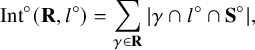$$ \begin{align*}\operatorname{Int}^\circ(\mathbf{R},l^\circ)=\sum_{\gamma\in\mathbf{R}}|\gamma\cap l^\circ\cap\mathbf{S}^\circ|,\end{align*} $$

and

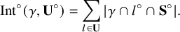$$ \begin{align*}\operatorname{Int}^\circ(\gamma,\mathbf{U}^\circ)=\sum_{l\in\mathbf{U}}|\gamma\cap l^\circ\cap\mathbf{S}^\circ|.\end{align*} $$

An arc $l\in \mathbf {U}$ is said to be

• ○ maximal if $\operatorname {Int}^\circ (\mathbf {R},l^\circ )\geq \operatorname {Int}^\circ (\mathbf {R},h^\circ )$ for any $h\in \mathbf {U}$ ;

• ○ double if l is homotopic to another arc in $\mathbf {U}$ (i.e., $l^\circ $ is a side of a self-folded triangle of $\mathbf {U}^\circ $ );

• ○ single if l is not homotopic to any other arc in $\mathbf {U}$ .

For a maximal $l\in \mathbf {U}$ , we also call $l^\circ $ maximal in $\mathbf {U}^\circ $ .

Denote by $\mathbf {U}^{non}$ the subset of $\mathbf {U}$ consisting of all arcs l such that $l^\circ $ is not the folded side of a self-folded triangle of $\mathbf {U}^\circ $ . By definition, any maximal arc in $\mathbf {U}$ is in $\mathbf {U}^{non}$ .

Next, we deal with two special cases. Recall that two tagged arcs $\gamma $ and l are called adjoint to each other if $\gamma (0),\gamma (1)\in \mathbf {P}$ and $l=\rho (\gamma )$ .

Lemma 5.19. Let $\gamma $ be a tagged arc in $\mathbf {R}$ not adjoint to any arc in $\mathbf {U}$ and such that $\operatorname {Int}^\circ (\gamma ,\mathbf {U}^\circ )=0$ . Then there exists a sequence of flips $f_{l_1},\cdots ,f_{l_k}$ such that $\gamma \in f_{l_k}\circ \cdots \circ f_{l_1}(\mathbf {U})$ .

Proof. Since $\operatorname {Int}^\circ (\gamma ,\mathbf {U}^\circ )=0$ , by Definition 4.2 and Remark 4.3, there is $l\in \mathbf {U}^{non}$ such that $\gamma ^{\mathbf {U}}$ , $l_s^\circ $ and $l^\circ $ form a contractible triangle clockwise, and with a certain orientation of $\gamma ^{\mathbf {U}}$ , we have $\gamma ^{\mathbf {U}}(1)=l^\circ (1)$ , $\kappa _{\gamma ^{\mathbf {U}}}(1)=-1$ , $\gamma ^{\mathbf {U}}(0)=l_s^\circ (1)$ and $\kappa _{\gamma ^{\mathbf {U}}}(0)=1$ if $\gamma ^{\mathbf {U}}(0)\in \mathbf {P}$ ; see Figure 14. So by Remark 4.5 (see also Figure 8), we have $b_{l,\mathbf {U}}(e^{op}(\gamma ))<0$ . Hence, by equation (5.3), $f_l(\mathbf {U})^\circ =f^-_{l^\circ }(\mathbf {U}^\circ )=\mathbf {U}^\circ \setminus \{l^\circ \}\cup \{f^-_{\mathbf {U}^\circ }(l^\circ )\}$ . Note that $\gamma ^{\mathbf {U}}(0)\neq \gamma ^{\mathbf {U}}(1)$ since $\gamma ^{\mathbf {U}}$ is a tagged arc.

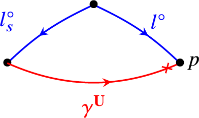
Figure 14 The case $\operatorname {Int}^\circ (\gamma ,\mathbf {U}^\circ )=0$ .

Let $p=\gamma ^{\mathbf {U}}(1)$ and $\mathbf {U}^\circ (p)$ be the set of arc segments of arcs in $\mathbf {U}^\circ $ that have p as an endpoint. We use the induction on $|\mathbf {U}^\circ (p)|$ .

If $|\mathbf {U}^\circ (p)|=1$ , then $l^\circ (0)\neq p$ and there is no other $h^\circ \in \mathbf {U}^\circ $ having p as an endpoint. This implies $\operatorname {Int}(\gamma ,h)=0$ for any $h\in \mathbf {U}\setminus \{l\}$ . Since $\gamma $ is $\mathbf {R}$ -standard and $\gamma \neq l$ (due to $\mathbf {R}\cap \mathbf {U}=\emptyset $ ), by Proposition 5.8, we have $f_{\mathbf {U}}(l)=\gamma $ , that is, $\gamma \in f_l(\mathbf {U})$ .

Suppose the assertion holds for $|\mathbf {U}^\circ (p)|<m$ with $k\geq 0$ and consider the case when $|\mathbf {U}^\circ (p)|=m$ . We have the following cases.

1. (1) $l^\circ (0)=l^\circ (1)$ , which contains the case that l is double; see the first picture in Figure 15. Then one endpoint of $f_{\mathbf {U}}(l)^\circ $ is $\gamma ^{\mathbf {U}}(0)\neq p$ . So $|f_l(\mathbf {U})^\circ (p)|<m$ , and we are done by the induction hypothesis.

   

   Figure 15 The cases of flip of $l^\circ $ for $\operatorname {Int}^\circ (\gamma ,\mathbf {U}^\circ )=0$ .

2. (2) $l^\circ (0)\neq l^\circ (1)$ and $l^\circ _t(0)\neq l^\circ _t(1)$ ; see the second picture of Figure 15. Then $f_{\mathbf {U}}(l)^\circ $ has $\gamma ^{\mathbf {U}}(0)$ and $l^\circ _t(0)$ as the endpoints, both of which are not p. So $|f_l(\mathbf {U})^\circ (p)|<m$ , and we are done by the induction hypothesis.

3. (3) $l^\circ (0)\neq l^\circ (1)$ and $l_t^\circ (0)=l_t^\circ (1)$ ; see the third picture in Figure 15. Then exactly one of the endpoints of $f_{\mathbf {U}}(l)^\circ $ is not p. So $|f_l(\mathbf {U})^\circ (p)|=m$ , and we go back to Case (1). Thus, we are done.

Lemma 5.20. Let $\gamma $ be a tagged arc in $\mathbf {R}$ adjoint to $l\in \mathbf {U}$ . Then l is the unique arc in $\mathbf {U}$ such that $b_{l,\mathbf {U}}(e^{op}(\gamma ))\neq 0$ . Moreover, if $\operatorname {Int}^\circ (\mathbf {R},l^\circ )\neq 0$ , then there exists a sequence of flips $f_{l_1},\cdots ,f_{l_k}$ such that $\gamma \in f_{l_k}\circ \cdots \circ f_{l_1}(\mathbf {U})$ .

Proof. By Remark 3.12, $e^{op}(\gamma )=e^{op}(\rho ^{-1}(l))=e(l)$ . So for any $h\in \mathbf {U}$ , $b_{h,\mathbf {U}}(e^{op}(\gamma ))=b_{h,\mathbf {U}}(e(l))$ , which by Corollary 3.18 is nonzero if and only if $h=l$ . Hence, l is the unique arc in $\mathbf {U}$ such that $b_{l,\mathbf {U}}(e^{op}(\gamma ))\neq 0$ . Indeed, we have $b_{l,\mathbf {U}}(e^{op}(\gamma ))<0$ by Corollary 3.18. Hence, by equation (5.3), $f_l(\mathbf {U})^\circ =f^-_{l^\circ }(\mathbf {U}^\circ )=\mathbf {U}^\circ \setminus \{l^\circ \}\cup \{f^-_{\mathbf {U}^\circ }(l^\circ )\}$ .

If $\operatorname {Int}^\circ (\mathbf {R},l^\circ )\neq 0$ , since l is adjoint to $\gamma \in \mathbf {R}$ , there is a self-folded triangle of $\mathbf {U}^\circ $ such that $l^\circ $ is its non-folded side. Let ${l^{\prime }}^\circ $ be the corresponding folded side. Then $\gamma $ is homotopic to ${l^{\prime }}^\circ \in f_l(\mathbf {U})^\circ $ . So $\operatorname {Int}^\circ (\gamma ,f_l(\mathbf {U})^\circ )=0$ . Since $l\notin f_l(\mathbf {U})$ , $\gamma $ is not adjoint to any arc in $f_l(\mathbf {U})$ , the assertion follows by Lemma 5.19.

Lemma 5.21. Let $\gamma \in \mathbf {R}$ . Suppose $\operatorname {Int}^\circ (\gamma ,\mathbf {U}^\circ )\neq 0$ . Then for any maximal tagged arc $l\in \mathbf {U}$ , any alternative intersection between $l^\circ $ and $\gamma $ is interior.

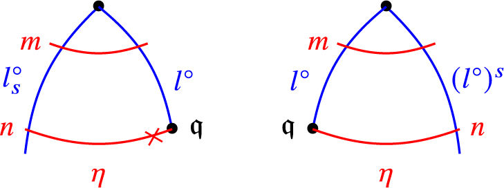
Figure 16 The case $l^\circ $ has an alternative intersection in $\mathbf {M}\cup \mathbf {P}$ with some $\gamma \in \mathbf {R}$ satisfying $\operatorname {Int}^\circ (\gamma ,\mathbf {U}^\circ )\neq 0$ .

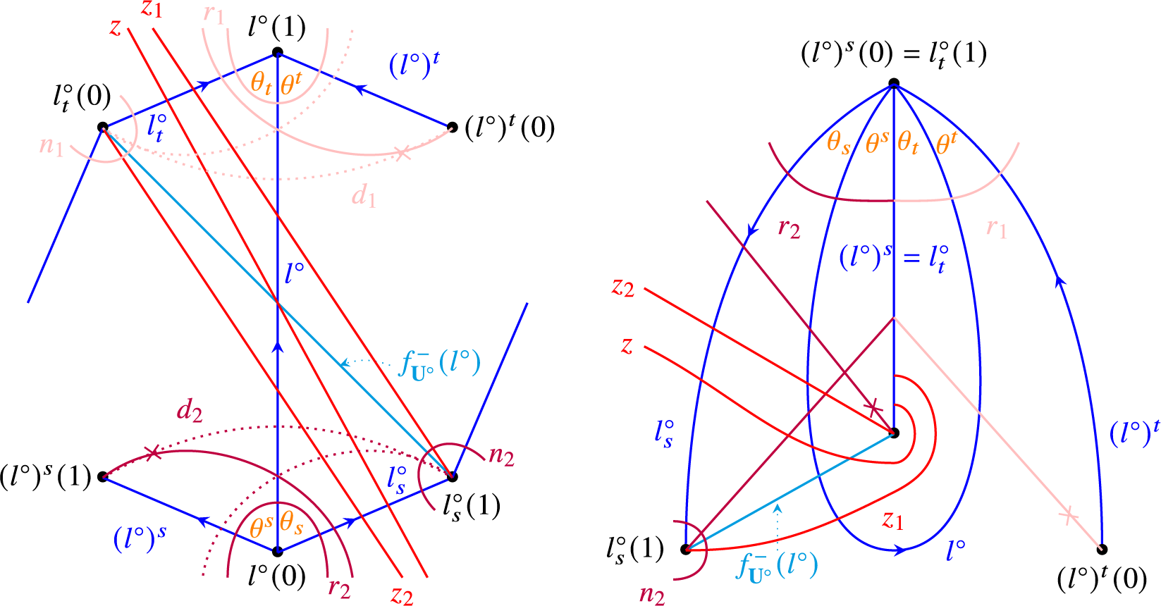
Figure 17 The case that no angle of $\mathbf {U}^\circ $ is formed by the two ends of $l^\circ $ .

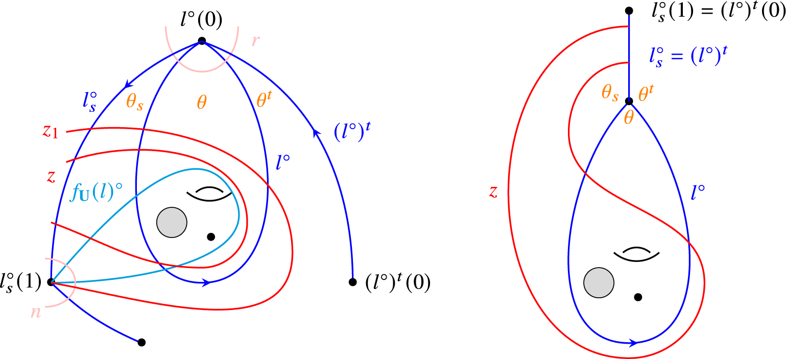
Figure 18 The case that one angle of $\mathbf {U}^\circ $ is formed by the two ends of $l^\circ $ .

Proof. Suppose conversely that $l^\circ $ has an alternative intersection $\mathfrak {q}\in \mathbf {M}\cup \mathbf {P}$ with $\gamma $ . Suppose without loss of generality that $\mathfrak {q}$ is negative. Let $\eta $ be the end arc segment of $\gamma ^{\mathbf {U}}$ incident to $\mathfrak {q}$ . Then by Remark 4.5, we are in one of the situations shown in Figure 16. In each case, let m be the number of non-end arc segments of arcs in $\mathbf {R}$ cutting out the same angle as $\eta $ and the number of end arc segments of arcs in $\mathbf {R}$ homotopic to $\eta $ . Then $\operatorname {Int}(\mathbf {R},l^\circ )=m$ and either $\operatorname {Int}(\mathbf {R},l^\circ _s)\geq m+n$ (see the left picture of Figure 16) or $\operatorname {Int}(\mathbf {R},(l^\circ )^s)\geq m+n$ (see the right picture of Figure 16), a contradiction to that l is maximal.

We need the following notions similarly as in [24]. For any arc $l\in \mathbf {U}$ , we say flipping l is convenient if $\operatorname {Int}^\circ (\mathbf {R},f_l(\mathbf {U})^\circ )<\operatorname {Int}^\circ (\mathbf {R},\mathbf {U}^\circ )$ , or neutral if $\operatorname {Int}^\circ (\mathbf {R},f_l(\mathbf {U})^\circ )=\operatorname {Int}^\circ (\mathbf {R},\mathbf {U}^\circ )$ , where

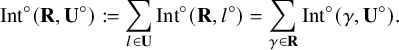$$ \begin{align*}\operatorname{Int}^\circ(\mathbf{R},\mathbf{U}^\circ):=\sum_{l\in\mathbf{U}}\operatorname{Int}^\circ(\mathbf{R},l^\circ)=\sum_{\gamma\in\mathbf{R}}\operatorname{Int}^\circ(\gamma,\mathbf{U}^\circ).\end{align*} $$

In what follows, for any $\gamma \in \mathbf {R}$ and a positive integer n, an n-arc segment of $\gamma $ is a segment of $\gamma $ formed by n arc segments.

Lemma 5.22. Let l be a maximal arc in $\mathbf {U}$ such that there is a negative (resp. positive) interior intersection $\mathfrak {q}$ between $l^\circ $ and some arc $\gamma \in \mathbf {R}$ . Then flipping l is either convenient or neutral. Moreover, if flipping l is neutral, then

1. (1) l is single,

2. (2) each alternative intersection in $\mathbf {S}^\circ $ between $l^\circ $ and an arc in $\mathbf {R}$ is not an endpoint of an end arc segment of the arc divided by $\mathbf {U}^\circ $ , and

3. (3) both $l^\circ _s$ and $l^\circ _t$ (resp. both $(l^\circ )^s$ and $(l^\circ )^t$ ) exist and are maximal if $\mathfrak {q}$ is negative (resp. positive).

Proof. We only deal with the case that $\mathfrak {q}$ is negative since the proof when $\mathfrak {q}$ is positive is similar. By equation (5.3), l is flip-convenient if $\operatorname {Int}^\circ (\mathbf {R},f^-_{\mathbf {U}^\circ }(l^\circ ))<\operatorname {Int}^\circ (\mathbf {R},l^\circ )$ , or flip-neutral if $\operatorname {Int}^\circ (\mathbf {R},f^-_{\mathbf {U}^\circ }(l^\circ ))=\operatorname {Int}^\circ (\mathbf {R},l^\circ )$ . We may assume that $f^-_{\mathbf {U}^\circ }(l^\circ )$ is not homotopic to any arc in $\mathbf {R}$ , because otherwise, $\operatorname {Int}^\circ (\mathbf {R},f^-_{\mathbf {U}^\circ }(l^\circ ))=0<\operatorname {Int}^\circ (\mathbf {R},l^\circ )$ . By Remark 4.5, we are in the situation shown in the second picture of the first row of Figure 8 with replacing $\gamma $ by $l^\circ $ and replacing $\delta $ by some arc $\gamma \in \mathbf {R}$ . There are the following cases.

1. (a) Suppose that there is no angle of $\mathbf {U}^\circ $ formed by $l^\circ $ and itself. In this case, the four angles $\theta _s,\theta ^s,\theta _t,\theta ^t$ (which are defined in Definition 5.4) are different. We shall use the following notations; see the first picture in Figure 17, where the label on each arc segment does not represent the arc segment itself, but rather the number of such arc segments.

   • – Let $r_1$ (resp. $r_2$ ) be the number of 2-arc segments of arcs in $\mathbf {R}$ that cut out the angles $\theta _t$ and $\theta ^t$ (resp. $\theta _s$ and $\theta ^s$ ) and whose arc segment cutting out $\theta _t$ (resp. $\theta _s$ ) does not have an endpoint in $\mathbf {M}\cup \mathbf {P}$ .

   • – Let $d_1$ (resp. $d_2$ ) be the number of 2-arc segments of arcs in $\mathbf {R}$ that cut out the angles $\theta _t$ and $\theta ^t$ (resp. $\theta _s$ and $\theta ^s$ ) and whose arc segment cutting out $\theta _t$ (resp. $\theta _s$ ) has an endpoint in $\mathbf {M}\cup \mathbf {P}$ ; see the dashed ones in the left picture of Figure 17.

   • – Let $n_1$ (resp. $n_2$ ) be the number of arc segments of arcs in $\mathbf {R}$ that cross $l^\circ _t$ (resp. $l^\circ _s$ ) and cut out the angle at $l^\circ _t(0)$ (resp. $l^\circ _s(1)$ ) clockwise from $l^\circ _t$ (resp. $l^\circ _s$ ).

   • – Let z be the number of 2-arc segments of arcs in $\mathbf {R}$ that cut out the angles $\theta _s$ and $\theta _t$ and are not incident to any point in $\mathbf {M}\cup \mathbf {P}$ .

   • – Let $z_1$ (resp. $z_2$ ) be the number of 2-arc segments of arcs in $\mathbf {R}$ that cut out the angles $\theta _s$ and $\theta _t$ and have one endpoint in $\mathbf {M}\cup \mathbf {P}$ .

   Then we have the following.

   $$\begin{align*}\operatorname{Int}^\circ(\mathbf{R},l^\circ)=r_1+r_2+d_1+d_2+z+z_1+z_2,\end{align*}$$
   $$\begin{align*}\operatorname{Int}^\circ(\mathbf{R},f^-_{\mathbf{U}^\circ}(l^\circ))=n_1+n_2+z,\end{align*}$$
   $$\begin{align*}\operatorname{Int}^\circ(\mathbf{R},l^\circ_t)=r_1+n_1+z+z_1,\end{align*}$$
   $$\begin{align*}\operatorname{Int}^\circ(\mathbf{R},l^\circ_s)=r_2+n_2+z+z_2.\end{align*}$$
   There are the following subcases.

   1. (1) Both $d_1$ and $d_2$ are nonzero. Since arcs in $\mathbf {R}$ do not cross each other in the interior, we have $n_1=n_2=0$ . So

      

   2. (2) Exactly one of $d_1$ and $d_2$ is not zero. Without loss of generality, suppose $d_1=0$ and $d_2\neq 0$ . Since arcs in $\mathbf {R}$ do not cross each other in the interior, we have $n_2=z=z_2=0$ , which implies $z_1\neq 0$ by the existence of a negative intersection $\mathfrak {q}$ . So

      

   3. (3) Both $d_1$ and $d_2$ are zero. So

      $$\begin{align*}\operatorname{Int}^\circ(\mathbf{R},l^\circ)-\operatorname{Int}^\circ(\mathbf{R},f^-_{\mathbf{U}^\circ}(l^\circ))=2\operatorname{Int}^\circ(\mathbf{R},l^\circ)-\operatorname{Int}^\circ(\mathbf{R},l^\circ_s)-\operatorname{Int}^\circ(\mathbf{R},l_t^\circ)\geq0.\end{align*}$$

   Hence, flipping l is either convenient or neutral. When flipping l is neutral, we have $d_1=d_2=0$ and $\operatorname {Int}^\circ (\mathbf {R},l^\circ )=\operatorname {Int}^\circ (\mathbf {R},l^\circ _s)=\operatorname {Int}^\circ (\mathbf {R},l_t^\circ )$ , which implies that both $l_s$ and $l_t$ exist and are maximal, and $r_2+z_2=n_1$ and $r_1+z_1=n_2$ . Since at least one of $n_1$ and $z_2$ (resp. $n_2$ and $z_1$ ) is zero, we have $z_1=z_2=0$ , $r_2=n_1$ and $r_1=n_2$ . If in addition, l is double, then with the chosen orientations, we have $(l^\circ )^s=l_t^\circ $ (with opposite orientations); see the second picture of Figure 17. Since the arc segment crossing $l_t^\circ $ and cutting out the angle at $l^\circ _t(0)$ clockwise from $l^\circ _t$ is a loop enclosing the puncture $l^\circ _t(0)$ , we have $n_1=0$ . So $r_2=0$ , which implies $z=0$ . So we have $z+z_1+z_2=0$ , which contradicts with that $\mathfrak {q}$ is negative.

2. (b) Otherwise, by Definition 4.2, $\gamma $ cuts out an angle $\theta $ formed by the different end segments of $l^\circ $ ; see the first picture in Figure 18. In this case, we have $l^\circ _s=l^\circ _t$ and $(l^\circ )^s=(l^\circ )^t$ , both with opposite orientations. The three angles $\theta ,\theta _s$ and $\theta ^t$ are different. We shall use the following notations; see the first picture in Figure 18.

   • – Let r be the number of 3-arc segments of arcs in $\mathbf {R}$ that cut out the angles $\theta _s$ , $\theta $ and $\theta ^t$ in order.

   • – Let n be the number of arc segments of arcs in $\mathbf {R}$ that cross $l^\circ _s$ and cut out the angle at $l^\circ _s(1)$ clockwise from $l^\circ _s$ .

   • – Let z be the number of 3-arc segments of arcs in $\mathbf {R}$ that cut out the angles $\theta _s$ , $\theta $ and $\theta _s$ in order and are not incident to any point in $\mathbf {M}\cup \mathbf {P}$ .

   • – Let $z_1$ be the number of 3-arc segments of arcs in $\mathbf {R}$ that cut out the angles $\theta _s$ , $\theta $ and $\theta _s$ in order and such that $l^\circ $ is the first or last arc in $\mathbf {U}$ they cross.

   Then

   $$\begin{align*}\operatorname{Int}^\circ(\mathbf{R},l^\circ)=2r+2z+2z_1,\end{align*}$$
   $$\begin{align*}\operatorname{Int}^\circ(\mathbf{R},f^-_{\mathbf{U}^\circ}(l^\circ))=2z+2n,\end{align*}$$
   $$\begin{align*}\operatorname{Int}^\circ(\mathbf{R},l^\circ_s)=r+n+2z+z_1.\end{align*}$$
   So we have
   $$\begin{align*}\begin{array}{rl} &\operatorname{Int}^\circ(\mathbf{R},l^\circ)-\operatorname{Int}^\circ(\mathbf{R},f^-_{\mathbf{U}^\circ}(l^\circ)) \\ =&2r+2z_1-2n\\ =&2(\operatorname{Int}^\circ(\mathbf{R},l^\circ)-\operatorname{Int}^\circ(\mathbf{R},l^\circ_s))\geq0. \end{array}\end{align*}$$
   Hence, flipping l is either convenient or neutral. When flipping l is neutral, we have $\operatorname {Int}^\circ (\mathbf {R},l^\circ )=\operatorname {Int}^\circ (\mathbf {R},l^\circ _s)$ , which implies that $l_s=l_t$ exists and is maximal, and $r+z_1=n$ . Since at least one of n and $z_1$ is zero, we have $z_1=0$ and $r=n$ . So $z\neq 0$ by the existence of a negative intersection $\mathfrak {q}$ . If in addition, l is double, then $l^\circ _s=(l^\circ )^t$ (with opposite orientations) be the folded side that is enclosed by $l^\circ $ ; see the second picture of Figure 18. Then any arc in $\mathbf {R}$ cuts out one of $\theta _s$ , $\theta $ and $\theta ^t$ can only cut out these three angles (by the $\mathbf {U}$ -co-standard property) and hence does not exist. This contradicts $z\neq 0$ .

Now we are ready to complete the proof of Lemma 5.15.

We use induction hypothesis on $\operatorname {Int}^\circ (\mathbf {R},\mathbf {U}^\circ )$ . For the starting case $\operatorname {Int}^\circ (\mathbf {R},\mathbf {U}^\circ )=0$ , since $\mathbf {R}$ is connected to the boundary, there is a tagged arc $\gamma ^{\prime }\in \mathbf {R}$ which has an endpoint in $\mathbf {M}$ . By definition, $\gamma ^{\prime }$ is not adjoint to any arc in $\mathbf {U}$ . So the assertion holds by Lemma 5.19.

Suppose the assertion holds when $\operatorname {Int}^\circ (\mathbf {R},\mathbf {U}^\circ )\leq k-1$ for some $k\geq 1$ , and consider the case when $\operatorname {Int}^\circ (\mathbf {R},\mathbf {U}^\circ )=k$ .

Let l be a maximal arc in $\mathbf {U}$ . Then $\operatorname {Int}^\circ (\mathbf {R},l^\circ )\neq 0$ . By Lemma 4.10, the set

$$ \begin{align*}\mathbf{R}(l):=\{\gamma\in\mathbf{R}\mid b_{l,\mathbf{U}}(e^{op}(\gamma))\neq 0\}\end{align*} $$

is nonempty. For any $\gamma \in \mathbf {R}(l)$ , if $\gamma $ is adjoint to $\mathbf {U}$ , then by Lemma 5.20, the assertion follows; if $\gamma $ is not adjoint to $\mathbf {U}$ and $\operatorname {Int}^\circ (\gamma ,\mathbf {U}^\circ )=0$ , then the assertion follows by Lemma 5.19. Hence, we only need to deal with the following case.

• (*) For any maximal $l\in \mathbf {U}$ and any $\gamma \in \mathbf {R}(l)$ , we have $\operatorname {Int}^\circ (\gamma ,\mathbf {U}^\circ )\neq 0$ .

Note that in this case, each $\gamma \in \mathbf {R}(l)$ has an alternative intersection with $l^\circ $ by Remark 4.5 and any such alternative intersection is interior by Lemma 5.21. So by Lemma 5.22, each maximal arc in $\mathbf {U}$ is either flip-convenient or flip-neutral. We use the induction on the minimum number m satisfying that there exists $\gamma \in \mathbf {R}$ which crosses $l_1^\circ ,\cdots ,l_m^\circ \in \mathbf {U}^\circ $ in succession, at $\mathfrak {q}_1,\cdots ,\mathfrak {q}_m$ , respectively, such that

1. (1) $\mathfrak {q}_1,\cdots ,\mathfrak {q}_m$ are interior, with only $\mathfrak {q}_m$ is alternative, and

2. (2) $l_1^\circ ,\cdots ,l_m^\circ $ are maximal in $\mathbf {U}$ , but the previous arc $l_0^\circ $ (if exists) in $\mathbf {U}^\circ $ that $\gamma $ crosses before $l_1^\circ $ is not.

Note that m is well defined because some arc in $\mathbf {R}$ has an interior alternative intersection with $\widetilde {l}^\circ $ for a maximal arc $\widetilde {l}\in \mathbf {U}$ , and hence, we can track along $\gamma $ to get a sequence satisfying the conditions above (although $\widetilde {l}$ may be one of $l_1,\cdots ,l_m$ ); see Figure 19.

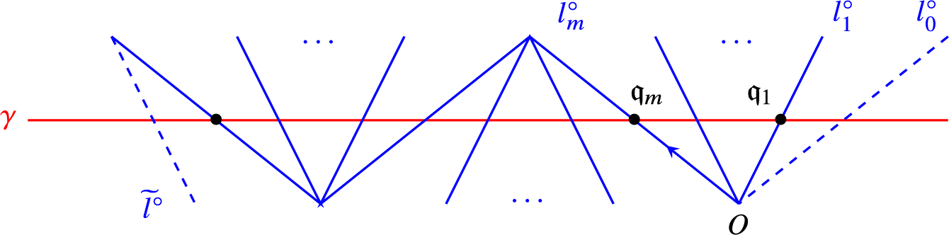
Figure 19 The conditions for the definition of m.

We denote $l=l_m$ and, without loss of generality, assume that $\mathfrak {q}_m$ is negative. For the starting case $m=1$ , if flipping l is neutral, then by Lemma 5.22, $\mathfrak {q}_1$ is not an endpoint of an end arc segment of $\gamma $ divided by $\mathbf {U}^\circ $ , and both $l_s^\circ $ and $l_t^\circ $ exist and are maximal. However, in this case, either $l_s^\circ $ or $l_t^\circ $ is $l_0^\circ $ which is not maximal, a contradiction. So flipping l is convenient, and the assertion holds by the induction hypothesis on $\operatorname {Int}^\circ (\mathbf {R},\mathbf {U}^\circ )$ .

Suppose the assertion holds when $m<k^{\prime }$ for some and consider the case when $m=k^{\prime }$ . Let O be the common endpoint of $l_1^\circ ,\cdots ,l_m^\circ $ and fix the orientation of $l_m^\circ $ with O as the starting point; see Figure 19. Since if flipping l is convenient then the assertion follows by the induction hypothesis on $\operatorname {Int}^\circ (\mathbf {R},\mathbf {U}^\circ )$ , in what follows, we assume that flipping l is neutral. By Lemma 5.22, l is single, $\mathfrak {q}_m$ is not an endpoint of an end arc segment of $\gamma $ divided by $\mathbf {U}^\circ $ , and both $l^\circ _s$ and $l^\circ _t$ exist and maximal. It follows that the next intersection $\mathfrak {q}_{m+1}$ of $\gamma $ with $\mathbf {U}^\circ $ after $\mathfrak {q}_m$ is also interior and with a maximal arc $l_{m+1}^\circ \in \mathbf {U}^\circ $ . For any $(l^{\prime })^\circ \in \mathbf {U}^\circ $ , let

$$ \begin{align*}\mathfrak{q}((l^{\prime})^\circ)=\{\mathfrak{q}_i\in (l^{\prime})^\circ\mid 1\leq i\leq m\}.\end{align*} $$

Note that we have $|\mathfrak {q}((l^{\prime })^\circ )|\leq 2$ , and the equality holds only if $(l^{\prime })^\circ $ is a loop at O. Depending on $l^\circ $ being whether $l^\circ _{m+1}$ , $l^\circ _{m-1}$ or not, there are the following three cases.

1. (1) Suppose $l^\circ =l_{m+1}^\circ $ . Then $l^\circ $ cuts out an angle $\theta $ by its two ends, $|\mathfrak {q}(l^\circ )|=1$ and $l^\circ _t=l^\circ _s=l^\circ _{m-1}$ . If $|\mathfrak {q}(l^\circ _s)|=2$ , then there is $1\leq i\leq m-2$ such that $l^\circ _{m-1}=l^\circ _i$ ; see the first picture in Figure 20. Similarly as in the case (b) in the proof of Lemma 5.22 (cf. the first picture of Figure 18), we denote

   

   Figure 20 The case $l^\circ =l_{m+1}^\circ $ .

   • ○ z the number of 3-arc segments of arcs in $\mathbf {R}$ that cut out the angle $\theta _s$ , $\theta $ and $\theta _s$ in order and are not incident to any point in $\mathbf {M}\cup \mathbf {P}$ ;

   • ○ r the number of 3-arc segments of arcs in $\mathbf {R}$ that cut out the angle $\theta ^t, \theta $ and $\theta _s$ , and

   • ○ n the number of arc segments of arcs in $\mathbf {R}$ that cross $l^\circ _s$ and cut out the angle at $l^\circ _s(1)$ clockwise from $l^\circ _s$ .

   Since any arcs in $\mathbf {R}$ have no intersections with each other, we have $n\geq r+1$ in this case. So

   $$\begin{align*}\operatorname{Int}(\mathbf{R},l^\circ)=2z+2r\end{align*}$$
   and
   
   which contradicts with $l^\circ $ is maximal. So $|\mathfrak {q}(l_s^\circ )|=1$ in this case, see the second picture in Figure 20. Then after flipping l, the value m decreases. If we are no longer in the case ( $\ast $ ), then we are already done. If we are still in the case ( $\ast $ ), then by applying the induction hypothesis on m, we get the assertion.

2. (2) Suppose $l^\circ =l^\circ _{m-1}$ . Then $l^\circ $ cuts out an angle $\theta $ by its two ends and $|\mathfrak {q}(l^\circ )|=2$ . So $l_t^\circ =l_s^\circ =l_{m+1}^\circ =l_{m-2}^\circ $ . Since flipping l is neutral, by Lemma 5.22, $l_{m+1}^\circ =l_s^\circ $ is maximal. But $l^\circ _0$ (if exists) is not maximal, so we have $m-2\geq 1$ . Then $|\mathfrak {q}(l_t^\circ )|\geq 1$ . The same argument in the above case $l^\circ =l^\circ _{m+1}$ can be used in the current case (see Figure 21) to get the required assertion.

   

   Figure 21 The case $l^\circ =l_{m-1}^\circ $ .

   

   Figure 22 The case $|\mathfrak {q}(l)|=|\mathfrak {q}(l_t)|=2$ .

   

   Figure 23 The case $|\mathfrak {q}(l)|=2$ , $|\mathfrak {q}(l_t)|=1$ .

   

   Figure 24 The case $|\mathfrak {q}(l^\circ )|=1$ , $|\mathfrak {q}(l_t^\circ )|=1$ .

3. (3) Suppose that $l^\circ $ is neither $l_{m+1}^\circ $ nor $l_{m-1}^\circ $ . Then $l^\circ _t=l^\circ _{m+1}$ , $l^\circ _s=l^\circ _{m-1}$ and $|\mathfrak {q}(l_t^\circ )|\leq |\mathfrak {q}(l^\circ )|$ . We shall use the notations in case (a) in the proof of Lemma 5.22; that is, we denote

   • ○ $r_1$ (resp. $r_2$ ) the number of 2-arc segments of arcs in $\mathbf {R}$ that cut out the angles $\theta _t$ and $\theta ^t$ (resp. $\theta _s$ and $\theta ^s$ ) and whose arc segment cutting out $\theta _t$ (resp. $\theta _s$ ) do not have an endpoint in $\mathbf {M}\cup \mathbf {P}$ ;

   • ○ $n_1$ (resp. $n_2$ ) the number of arc segments of arcs in $\mathbf {R}$ that cross $l^\circ _t$ (resp. $l^\circ _s$ ) and cut out the angle at $l^\circ _t(0)$ (resp. $l^\circ _s(1)$ ) clockwise from $l^\circ _t$ (resp. $l^\circ _s$ );

   • ○ z the number of 2-arc segments of arcs in $\mathbf {R}$ that cut out the angles $\theta _s$ and $\theta _t$ and are not incident to any point in $\mathbf {M}\cup \mathbf {P}$ .

   There are the following cases.

   1. (a) $|\mathfrak {q}(l^\circ )|=2$ , that is, there is $1\leq k\leq m-2$ such that $l^\circ =l_k^\circ $ . If $k=1$ , then $l^\circ _0$ exists and is the same as $l^\circ _{m+1}$ . Note that $l^\circ _0$ is not maximal but $l^\circ _{m+1}$ is maximal, a contradiction. So we have $k\neq 1$ and $l^\circ _{m+1}=l^\circ _{k-1}$ . Then $|\mathfrak {q}(l^\circ _t)|\geq 1$ . If $|\mathfrak {q}(l^\circ _t)|=2$ , then there is $1\leq i< m$ , $i\neq k-1,k$ , such that $l^\circ _{k-1}=l^\circ _i$ ; see the pictures of Figure 22, where the left is for $1\leq i<k-1$ and the right is for $k<i<m$ . Since arcs in $\mathbf {R}$ do not cross each other in the interior, we have $n_1\geq r_2+1$ . Hence,

      $$\begin{align*}\operatorname{Int}(\mathbf{R},l^\circ)=r_1+r_2+z,\end{align*}$$
      and
      
      contradicts to $l^\circ $ is maximal. So in this case, we have $|\mathfrak {q}(l^\circ _t)|=1$ (see Figure 23), where the left picture is for $|\mathfrak {q}(l_{m-1}^\circ )|=1$ and the right one is for $|\mathfrak {q}(l_{m-1}^\circ )|=2$ . Then after flipping l, the value m decreases 2 for the left picture and decreases 1 for the right picture. If we are no longer in the case $(\ast )$ , then we are already done. If we are still in the case $(\ast )$ , then applying the induction hypothesis on m, we get the assertion.

   2. (b) $|\mathfrak {q}(l^\circ )|=1$ . Then $|\mathfrak {q}(l_{m+1}^\circ )|\leq 1$ . If $|\mathfrak {q}(l_{m+1}^\circ )|=1$ , then there is $1\leq i\leq m-1$ such that $l_{m+1}^\circ =l_i^\circ $ ; see Figure 24. Since arcs in $\mathbf {R}$ do not cross each other in the interior, we have $n_1\geq r_2+1$ . Hence,

      $$\begin{align*}\operatorname{Int}(\mathbf{R},l^\circ)=r_1+r_2+z,\end{align*}$$
      and
      
      contradicts to $l^\circ $ is maximal. So in this case, we have $|\mathfrak {q}(l^\circ _{m+1})|=0$ . There are the following two subcases

      1. (i) $|\mathfrak {q}(l^\circ _{m-1})|=1$ ; see the first picture in Figure 25. Then after flipping l, the value m decreases $1$ . If we are no longer in the case $(\ast )$ , then we are already done. If we are still in the case $(\ast )$ , then applying the induction hypothesis on m, we get the assertion.

         

         Figure 25 The case $|\mathfrak {q}(l^\circ )|=1$ , $|\mathfrak {q}(l_{m+1}^\circ )|=0$ .

      2. (ii) $|\mathfrak {q}(l^\circ _{m-1})|=2$ , that is, there is $1\leq i< m-1$ such that $l_{m-1}^\circ =l_i^\circ $ ; see the second picture in Figure 25. Then after flipping l, the value m does not change. If we are no longer in the case $(\ast )$ , then we are already done. If we are still in the case $(\ast )$ , then we go back to cases (2) and (3.a). So we are also done.