


1 Introduction
Let G be an almost simple algebraic group over $\mathbb {C}$
and let
$\mathbb {C}$
and let $\operatorname {\mathrm {\mathtt {Gr}}}_G$
be the affine Grassmannian of G. The geometry of the affine Grassmannian is related to integral highest weight representations of Kac-Moody algebras via the affine Borel-Weil theorem. Similarly, the geometry of affine Schubert varieties are closely related to affine Demazure modules.
$\operatorname {\mathrm {\mathtt {Gr}}}_G$
be the affine Grassmannian of G. The geometry of the affine Grassmannian is related to integral highest weight representations of Kac-Moody algebras via the affine Borel-Weil theorem. Similarly, the geometry of affine Schubert varieties are closely related to affine Demazure modules.
Let T be a maximal torus in G and let $X_*(T)^+$
be the set of dominant coweights. For any
$X_*(T)^+$
be the set of dominant coweights. For any $\lambda \in X_*(T)^+$
, let
$\lambda \in X_*(T)^+$
, let $\overline {\operatorname {\mathrm {\mathtt {Gr}}}}_G^\lambda $
be the associated affine Schubert variety in
$\overline {\operatorname {\mathrm {\mathtt {Gr}}}}_G^\lambda $
be the associated affine Schubert variety in $\operatorname {\mathrm {\mathtt {Gr}}}_G$
, which is the closure of the
$\operatorname {\mathrm {\mathtt {Gr}}}_G$
, which is the closure of the $G(\mathcal {O})$
-orbit
$G(\mathcal {O})$
-orbit ${\operatorname {\mathrm {\mathtt {Gr}}}}_G^\lambda $
, where
${\operatorname {\mathrm {\mathtt {Gr}}}}_G^\lambda $
, where $\mathcal {O}=\mathbb {C}[[t]]$
. Evens-Mirković [Reference Evens and MirkovićEM] and Malkin-Ostrik-Vybornov [Reference Malkin, Ostrik and VybornovMOV] proved that the smooth locus of
$\mathcal {O}=\mathbb {C}[[t]]$
. Evens-Mirković [Reference Evens and MirkovićEM] and Malkin-Ostrik-Vybornov [Reference Malkin, Ostrik and VybornovMOV] proved that the smooth locus of $\overline {\operatorname {\mathrm {\mathtt {Gr}}}}_G^\lambda $
is exactly the open Schubert cell
$\overline {\operatorname {\mathrm {\mathtt {Gr}}}}_G^\lambda $
is exactly the open Schubert cell $\operatorname {\mathrm {\mathtt {Gr}}}_G^\lambda $
. Zhu [Reference ZhuZh1] proved that there is a duality between the affine Demazure modules and the coordinate ring of the T-fixed point subschemes of affine Schubert varieties when G is of type A and D, and in many cases of the exceptional types
$\operatorname {\mathrm {\mathtt {Gr}}}_G^\lambda $
. Zhu [Reference ZhuZh1] proved that there is a duality between the affine Demazure modules and the coordinate ring of the T-fixed point subschemes of affine Schubert varieties when G is of type A and D, and in many cases of the exceptional types $E_6, E_7$
and
$E_6, E_7$
and $E_8$
. As a consequence, this gives another approach to determine the smooth locus of
$E_8$
. As a consequence, this gives another approach to determine the smooth locus of $\overline {\operatorname {\mathrm {\mathtt {Gr}}}}_G^\lambda $
for type
$\overline {\operatorname {\mathrm {\mathtt {Gr}}}}_G^\lambda $
for type $A,D$
and many cases of type E.
$A,D$
and many cases of type E.
In this paper, we study a connection between the geometry of twisted affine Schubert varieties and twisted affine Demazure modules. Following the method of Zhu in [Reference ZhuZh1], we will use the weight multiplicities of twisted affine Demazure modules to determine the smooth locus of twisted affine Schubert varieties.
Let G be an almost simple algebraic group of simply-laced or adjoint type with the action of a ‘standard’ automorphism $\sigma $
of order m, defined in Section 2.1. When G is not of type
$\sigma $
of order m, defined in Section 2.1. When G is not of type $A_{2\ell }$
,
$A_{2\ell }$
, $\sigma $
is just a diagram automorphism. Assume that
$\sigma $
is just a diagram automorphism. Assume that $\sigma $
acts on
$\sigma $
acts on $\mathcal {O}$
by rotation of order m. Let
$\mathcal {O}$
by rotation of order m. Let ${\mathscr {G}}$
be the
${\mathscr {G}}$
be the $\sigma $
-fixed point subgroup scheme of the Weil restriction group
$\sigma $
-fixed point subgroup scheme of the Weil restriction group $\mathrm {Res}_{\mathcal {O}/ \bar {\mathcal {O}} }(G_{\mathcal {O}})$
, where
$\mathrm {Res}_{\mathcal {O}/ \bar {\mathcal {O}} }(G_{\mathcal {O}})$
, where $\bar {\mathcal {O}} =\mathbb {C}[[t^m]]$
. Then
$\bar {\mathcal {O}} =\mathbb {C}[[t^m]]$
. Then ${\mathscr {G}}$
is a special parahoric group scheme over
${\mathscr {G}}$
is a special parahoric group scheme over $\bar {\mathcal {O}}$
in the sense of Bruhat-Tits. One may define the affine Grassmannian
$\bar {\mathcal {O}}$
in the sense of Bruhat-Tits. One may define the affine Grassmannian $\operatorname {\mathrm {\mathtt {Gr}}}_{\mathscr {G}} $
of
$\operatorname {\mathrm {\mathtt {Gr}}}_{\mathscr {G}} $
of ${\mathscr {G}} $
. Following [Reference Pappas and RapoportPR, Reference ZhuZh2], we will call it a twisted affine Grassmannian. For any
${\mathscr {G}} $
. Following [Reference Pappas and RapoportPR, Reference ZhuZh2], we will call it a twisted affine Grassmannian. For any $\bar {\lambda }$
the image of a dominant coweight
$\bar {\lambda }$
the image of a dominant coweight $\lambda $
in the set
$\lambda $
in the set $X_*(T)_\sigma $
of
$X_*(T)_\sigma $
of $\sigma $
-coinvariants of
$\sigma $
-coinvariants of $X_*(T)$
, the twisted affine Grassmannian
$X_*(T)$
, the twisted affine Grassmannian $\operatorname {\mathrm {\mathtt {Gr}}}_{\mathscr {G}} $
and twisted affine Schubert varieties
$\operatorname {\mathrm {\mathtt {Gr}}}_{\mathscr {G}} $
and twisted affine Schubert varieties $\overline {\operatorname {\mathrm {\mathtt {Gr}}}}_{\mathscr {G}} ^{\bar {\lambda }} $
share many similar properties with the usual affine Grassmannian
$\overline {\operatorname {\mathrm {\mathtt {Gr}}}}_{\mathscr {G}} ^{\bar {\lambda }} $
share many similar properties with the usual affine Grassmannian $\operatorname {\mathrm {\mathtt {Gr}}}_G$
and affine Schubert varieties. For instance, a version of the geometric Satake isomorphism for
$\operatorname {\mathrm {\mathtt {Gr}}}_G$
and affine Schubert varieties. For instance, a version of the geometric Satake isomorphism for ${\mathscr {G}}$
was proved by Zhu in [Reference ZhuZh3].
${\mathscr {G}}$
was proved by Zhu in [Reference ZhuZh3].
In the literature, special parahoric group schemes are parametrized by special vertices on local Dynkin diagrams. In this paper, our approach is more Kac-Moody theoretic. For this reason, we use the terminology of affine Dynkin diagrams instead of local Dynkin diagrams. Following [Reference Haines and RicharzHR], there are two special parahoric group schemes for $A_{2\ell }^{(2)}$
, and in this case, the parahoric group scheme
$A_{2\ell }^{(2)}$
, and in this case, the parahoric group scheme ${\mathscr {G}}$
that we consider is special but not absolutely special. We prove Theorem 4.5 in Section 4, which asserts the following.
${\mathscr {G}}$
that we consider is special but not absolutely special. We prove Theorem 4.5 in Section 4, which asserts the following.
Theorem 1.1. For any special parahoric group scheme ${\mathscr {G}} $
induced from a standard automorphism
${\mathscr {G}} $
induced from a standard automorphism $\sigma $
, the following restriction is an isomorphism:
$\sigma $
, the following restriction is an isomorphism:
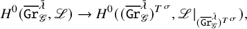 $$\begin{align*}H^0(\overline{\operatorname{\mathrm{\mathtt{Gr}}}}_{\mathscr{G}}^{\bar{\lambda}}, \mathscr{L}) \rightarrow H^0((\overline{\operatorname{\mathrm{\mathtt{Gr}}}}_{\mathscr{G}}^{\bar{\lambda}})^{T^{\sigma}}, \mathscr{L}|_{(\overline{\operatorname{\mathrm{\mathtt{Gr}}}}_{\mathscr{G}}^{\bar{\lambda}})^{T^{\sigma}}}) , \end{align*}$$
where $\mathscr {L}$
is the level one line bundle on
$\mathscr {L}$
is the level one line bundle on $\operatorname {\mathrm {\mathtt {Gr}}}_{\mathscr {G}} $
,
$\operatorname {\mathrm {\mathtt {Gr}}}_{\mathscr {G}} $
, $T^\sigma $
is the
$T^\sigma $
is the $\sigma $
-fixed point subgroup of a
$\sigma $
-fixed point subgroup of a $\sigma $
-stable maximal torus T in G and
$\sigma $
-stable maximal torus T in G and $(\overline {\operatorname {\mathrm {\mathtt {Gr}}}}_{\mathscr {G}}^{\bar {\lambda }})^{T^{\sigma }}$
is the
$(\overline {\operatorname {\mathrm {\mathtt {Gr}}}}_{\mathscr {G}}^{\bar {\lambda }})^{T^{\sigma }}$
is the $T^\sigma $
-fixed point subsheme of
$T^\sigma $
-fixed point subsheme of $\overline {\operatorname {\mathrm {\mathtt {Gr}}}}_{\mathscr {G}}^{\bar {\lambda }}$
.
$\overline {\operatorname {\mathrm {\mathtt {Gr}}}}_{\mathscr {G}}^{\bar {\lambda }}$
.
The above theorem can not be extended to the absolutely special parahoric group scheme of type $A_{2\ell }^{(2)}$
, as there is no level one line bundle on
$A_{2\ell }^{(2)}$
, as there is no level one line bundle on $\operatorname {\mathrm {\mathtt {Gr}}}_{\mathscr {G}}$
(cf. [Reference ZhuZh2]). This theorem extends Zhu’s duality to the twisted setting. The dual
$\operatorname {\mathrm {\mathtt {Gr}}}_{\mathscr {G}}$
(cf. [Reference ZhuZh2]). This theorem extends Zhu’s duality to the twisted setting. The dual $H^0(\overline {\operatorname {\mathrm {\mathtt {Gr}}}}_{\mathscr {G}}^{\bar {\lambda }}, \mathscr {L})^\vee $
is a twisted affine Demazure module; see Theorem 3.10. Hence, Theorem 1.1 is a duality between twisted affine Demazure modules and the coordinate rings of the
$H^0(\overline {\operatorname {\mathrm {\mathtt {Gr}}}}_{\mathscr {G}}^{\bar {\lambda }}, \mathscr {L})^\vee $
is a twisted affine Demazure module; see Theorem 3.10. Hence, Theorem 1.1 is a duality between twisted affine Demazure modules and the coordinate rings of the $T^\sigma $
-fixed point subschemes of twisted affine Schubert varieties. One of the motivations of the work of Zhu [Reference ZhuZh1] is to give a geometric realization of Frenkel-Kac vertex operator construction for untwisted simply-laced affine Lie algebras. The analogue of Frenkel-Kac construction for twisted affine Lie algebras also exists in literature; see [Reference Bernard and Thierry-MiegBT, Reference Frenkel, Lepowsky and MeurmanFLM]. In fact, our Theorem 1.1 implies a geometric Frenkel-Kac isomorphism; see Theorem 4.9.
$T^\sigma $
-fixed point subschemes of twisted affine Schubert varieties. One of the motivations of the work of Zhu [Reference ZhuZh1] is to give a geometric realization of Frenkel-Kac vertex operator construction for untwisted simply-laced affine Lie algebras. The analogue of Frenkel-Kac construction for twisted affine Lie algebras also exists in literature; see [Reference Bernard and Thierry-MiegBT, Reference Frenkel, Lepowsky and MeurmanFLM]. In fact, our Theorem 1.1 implies a geometric Frenkel-Kac isomorphism; see Theorem 4.9.
As a consequence of Theorem 1.1, we obtain Theorem 4.10 and Theorem 4.11, which asserts the following.
Theorem 1.2.
-
1. If ${\mathscr {G}}$
is not of type
$A_{2\ell }^{(2)}$
, then for any
$\bar {\lambda }\in X_*(T)_\sigma $
, the smooth locus of the twisted affine Schubert variety
$\overline {\operatorname {\mathrm {\mathtt {Gr}}}}_{\mathscr {G}} ^{\bar {\lambda }}$
is exactly the open cell
$\operatorname {\mathrm {\mathtt {Gr}}}_{\mathscr {G}} ^{\bar {\lambda }}$
.
${\mathscr {G}}$
is not of type
$A_{2\ell }^{(2)}$
, then for any
$\bar {\lambda }\in X_*(T)_\sigma $
, the smooth locus of the twisted affine Schubert variety
$\overline {\operatorname {\mathrm {\mathtt {Gr}}}}_{\mathscr {G}} ^{\bar {\lambda }}$
is exactly the open cell
$\operatorname {\mathrm {\mathtt {Gr}}}_{\mathscr {G}} ^{\bar {\lambda }}$
. -
2. If
${\mathscr {G}}$
is special but not absolutely special of type
$A_{2\ell }^{(2)}$
, then for any
$\bar {\lambda }\in X_*(T)_\sigma $
, the smooth locus of the twisted affine Schubert variety
$\overline {\operatorname {\mathrm {\mathtt {Gr}}}}_{\mathscr {G}} ^{\bar {\lambda }}$
is the union of
$\operatorname {\mathrm {\mathtt {Gr}}}_{\mathscr {G}} ^{\bar {\lambda }}$
and possibly some other cells
$\operatorname {\mathrm {\mathtt {Gr}}}_{\mathscr {G}} ^{\bar {\mu }}$
, which are completely determined in Theorem 4.11.


When ${\mathscr {G}}$
is absolutely special of type
${\mathscr {G}}$
is absolutely special of type $A^{(2)}_{2\ell }$
, our method is not applicable, as there is no level one line bundle on the affine Grassmannian of
$A^{(2)}_{2\ell }$
, our method is not applicable, as there is no level one line bundle on the affine Grassmannian of ${\mathscr {G}}$
. Nevertheless, Richarz already proved in his Diploma [Reference RicharzRi2] that in this case, the smooth locus of any twisted affine Schubert variety is the open cell; see Remark 4.12. Thus, our Theorem 1.2 confirms a conjecture of Haines-Richarz [Reference Haines and RicharzHR, Conjecture 5.4]. Beyond that, we also completely determine the smooth locus of twisted affine Schubert varieties for special but not absolutely special parahoric group scheme
${\mathscr {G}}$
. Nevertheless, Richarz already proved in his Diploma [Reference RicharzRi2] that in this case, the smooth locus of any twisted affine Schubert variety is the open cell; see Remark 4.12. Thus, our Theorem 1.2 confirms a conjecture of Haines-Richarz [Reference Haines and RicharzHR, Conjecture 5.4]. Beyond that, we also completely determine the smooth locus of twisted affine Schubert varieties for special but not absolutely special parahoric group scheme ${\mathscr {G}}$
of type
${\mathscr {G}}$
of type $A_{2\ell }^{(2)}$
. Richarz studied the twisted affine Schubert varieties in [Reference RicharzRi2] and determined their smooth loci in the case of absolutely special group schemes of type
$A_{2\ell }^{(2)}$
. Richarz studied the twisted affine Schubert varieties in [Reference RicharzRi2] and determined their smooth loci in the case of absolutely special group schemes of type $A_{2\ell }^{(2)}$
and the special parahoric group scheme of type
$A_{2\ell }^{(2)}$
and the special parahoric group scheme of type $A_{2\ell -1}^{(2)}$
. It is also worthwhile to mention that the smooth locus of the quasi-minuscule Schubert variety for
$A_{2\ell -1}^{(2)}$
. It is also worthwhile to mention that the smooth locus of the quasi-minuscule Schubert variety for $D^{(3)}_{4}$
is determined by Haines-Richarz in [Reference Haines and RicharzHR] by rather lengthy computations. In fact, one can define special parahoric group schemes over any base field
$D^{(3)}_{4}$
is determined by Haines-Richarz in [Reference Haines and RicharzHR] by rather lengthy computations. In fact, one can define special parahoric group schemes over any base field $\mathrm {k}$
of any characteristic, and the twisted Schubert variety
$\mathrm {k}$
of any characteristic, and the twisted Schubert variety $\overline {\operatorname {\mathrm {\mathtt {Gr}}}}_{\mathscr {G}}^{\bar {\lambda }}$
over the field
$\overline {\operatorname {\mathrm {\mathtt {Gr}}}}_{\mathscr {G}}^{\bar {\lambda }}$
over the field $\mathrm {k}$
. By the works [Reference Haines, Lourenço and RicharzHLR, Reference Haines and RicharzHR, Reference LourençoLo], Theorem 1.2 remains true for normal twisted Schubert varieties over any field
$\mathrm {k}$
. By the works [Reference Haines, Lourenço and RicharzHLR, Reference Haines and RicharzHR, Reference LourençoLo], Theorem 1.2 remains true for normal twisted Schubert varieties over any field $\mathrm {k}$
(Schubert varieties are always normal if the characteristic is not bad).
$\mathrm {k}$
(Schubert varieties are always normal if the characteristic is not bad).
To prove Theorem 1.1, one ingredient is Theorem 4.2 in Section 4, which asserts that the $T^\sigma $
-fixed point ind-subscheme
$T^\sigma $
-fixed point ind-subscheme $(\operatorname {\mathrm {\mathtt {Gr}}}_{{\mathscr {G}} })^{T^\sigma } $
is isomorphic to the affine Grassmannian
$(\operatorname {\mathrm {\mathtt {Gr}}}_{{\mathscr {G}} })^{T^\sigma } $
is isomorphic to the affine Grassmannian $\operatorname {\mathrm {\mathtt {Gr}}}_{\mathscr {T}}$
, where
$\operatorname {\mathrm {\mathtt {Gr}}}_{\mathscr {T}}$
, where ${\mathscr {T}}$
is the
${\mathscr {T}}$
is the $\sigma $
-fixed point subscheme of the Weil restriction group
$\sigma $
-fixed point subscheme of the Weil restriction group $\mathrm {Res}_{\mathcal {O}/ \bar {\mathcal {O}} }(T_{\mathcal {O}})$
.
$\mathrm {Res}_{\mathcal {O}/ \bar {\mathcal {O}} }(T_{\mathcal {O}})$
.
Let $\pi : \mathbb {P}^1\to \bar {\mathbb {P}}^1$
be the map given by
$\pi : \mathbb {P}^1\to \bar {\mathbb {P}}^1$
be the map given by $t\mapsto t^m$
, where
$t\mapsto t^m$
, where $ \bar {\mathbb {P}}^1$
is a copy of
$ \bar {\mathbb {P}}^1$
is a copy of $\mathbb {P}^1$
. Another main ingredient of the proof of Theorem 1.1 is the construction of the level one line bundle
$\mathbb {P}^1$
. Another main ingredient of the proof of Theorem 1.1 is the construction of the level one line bundle $\mathcal {L}$
on the moduli stack
$\mathcal {L}$
on the moduli stack $\mathrm {Bun}_{ \mathcal {G}} $
of
$\mathrm {Bun}_{ \mathcal {G}} $
of $\mathcal {G}$
-torsors, where
$\mathcal {G}$
-torsors, where $ \mathcal {G}$
is the parahoric Bruhat-Tits group scheme obtained as the
$ \mathcal {G}$
is the parahoric Bruhat-Tits group scheme obtained as the $\sigma $
-fixed subgroup scheme of the Weil restriction group
$\sigma $
-fixed subgroup scheme of the Weil restriction group $\mathrm {Res}_{ \mathbb {P}^1 /\bar {\mathbb {P}}^1 }(G_{\mathbb {P}^1 }) $
with G being simply-connected. This is achieved in Section 3. It is known that the level one line bundle on
$\mathrm {Res}_{ \mathbb {P}^1 /\bar {\mathbb {P}}^1 }(G_{\mathbb {P}^1 }) $
with G being simply-connected. This is achieved in Section 3. It is known that the level one line bundle on $\mathrm {Bun}_{\mathcal {G}}$
does not necessarily exist for an arbitary parahoric Bruhat-Tits group scheme
$\mathrm {Bun}_{\mathcal {G}}$
does not necessarily exist for an arbitary parahoric Bruhat-Tits group scheme $\mathcal {G}$
over a smooth projective curve – for example when
$\mathcal {G}$
over a smooth projective curve – for example when $\mathcal {G}$
is of type
$\mathcal {G}$
is of type $A_{2\ell }$
; cf. [Reference HeinlothHe, Remark 19 (4)] [Reference ZhuZh2, Proposition 4.1]. In Theorem 3.13, when
$A_{2\ell }$
; cf. [Reference HeinlothHe, Remark 19 (4)] [Reference ZhuZh2, Proposition 4.1]. In Theorem 3.13, when $\sigma $
is standard, we prove that there exists a level one line bundle
$\sigma $
is standard, we prove that there exists a level one line bundle $\mathcal {L}$
on the moduli stack
$\mathcal {L}$
on the moduli stack $\mathrm {Bun}_{ \mathcal {G}} $
of
$\mathrm {Bun}_{ \mathcal {G}} $
of $\mathcal {G}$
-torsors. Following the method of Sorger in [Reference SorgerSo], we use the nonvanishing of twisted conformal blocks to construct this line bundle on
$\mathcal {G}$
-torsors. Following the method of Sorger in [Reference SorgerSo], we use the nonvanishing of twisted conformal blocks to construct this line bundle on $\mathrm { Bun}_{\mathcal {G}}$
, where the general theory of twisted conformal blocks was recently developed by Hong-Kumar in [Reference Hong and KumarHK].
$\mathrm { Bun}_{\mathcal {G}}$
, where the general theory of twisted conformal blocks was recently developed by Hong-Kumar in [Reference Hong and KumarHK].
By the work of Zhu in [Reference ZhuZh2], for each dominant coweight $\lambda $
, one can construct a global Schubert variety
$\lambda $
, one can construct a global Schubert variety $\overline {\operatorname {\mathrm {\mathtt {Gr}}}}_{\mathcal {G}}^\lambda $
, which is flat over
$\overline {\operatorname {\mathrm {\mathtt {Gr}}}}_{\mathcal {G}}^\lambda $
, which is flat over $\mathbb {P}^1$
. The fiber over the origin is the twisted affine Schubert variety
$\mathbb {P}^1$
. The fiber over the origin is the twisted affine Schubert variety $\overline {\operatorname {\mathrm {\mathtt {Gr}}}}_{\mathscr {G}}^{\bar {\lambda }}$
, and the fiber over a generic point is isomorphic to the usual affine Schubert variety
$\overline {\operatorname {\mathrm {\mathtt {Gr}}}}_{\mathscr {G}}^{\bar {\lambda }}$
, and the fiber over a generic point is isomorphic to the usual affine Schubert variety $\overline {\operatorname {\mathrm {\mathtt {Gr}}}}_{G}^{\lambda }$
. With the level one line bundle on
$\overline {\operatorname {\mathrm {\mathtt {Gr}}}}_{G}^{\lambda }$
. With the level one line bundle on $\mathrm {Bun}_{ \mathcal {G}} $
when
$\mathrm {Bun}_{ \mathcal {G}} $
when $\mathcal {G}$
is simply-connected, we can construct the level one line bundle on the global affine Schubert variety
$\mathcal {G}$
is simply-connected, we can construct the level one line bundle on the global affine Schubert variety $\overline {\operatorname {\mathrm {\mathtt {Gr}}}}_{\mathcal {G}}^\lambda $
for
$\overline {\operatorname {\mathrm {\mathtt {Gr}}}}_{\mathcal {G}}^\lambda $
for $\mathcal {G}$
being either simply-connected or adjoint. The main idea of this paper is that our duality theorem for twisted affine Schubert varieties can follow from Zhu’s duality theorem for usual affine Schubert varieties via the level one line bundle on the global affine Schubert variety
$\mathcal {G}$
being either simply-connected or adjoint. The main idea of this paper is that our duality theorem for twisted affine Schubert varieties can follow from Zhu’s duality theorem for usual affine Schubert varieties via the level one line bundle on the global affine Schubert variety $\overline {\operatorname {\mathrm {\mathtt {Gr}}}}_G^{\lambda }$
.
$\overline {\operatorname {\mathrm {\mathtt {Gr}}}}_G^{\lambda }$
.
The proof of Theorem 1.1 relies on the duality theorem of Zhu in the untwisted case. However, Zhu only established the duality in the case of type $A, D$
and some cases of type
$A, D$
and some cases of type $E_6,E_7.E_8$
. To fully establish Theorem 1.1, we need to prove the duality theorem for
$E_6,E_7.E_8$
. To fully establish Theorem 1.1, we need to prove the duality theorem for $E_6$
in the untwisted setting. In the case of
$E_6$
in the untwisted setting. In the case of $E_6$
, the duality has been established by Zhu when
$E_6$
, the duality has been established by Zhu when $\lambda $
is the fundamental coweight
$\lambda $
is the fundamental coweight $\check {\omega }_1,\check {\omega }_2, \check {\omega }_3, \check {\omega }_5, \check {\omega }_6$
(Bourbaki labelling), and Zhu also showed that the duality theorem will hold in general if the duality also holds for
$\check {\omega }_1,\check {\omega }_2, \check {\omega }_3, \check {\omega }_5, \check {\omega }_6$
(Bourbaki labelling), and Zhu also showed that the duality theorem will hold in general if the duality also holds for $\check {\omega }_4$
, which is the most difficult case. In Section 5, we establish the duality theorem for
$\check {\omega }_4$
, which is the most difficult case. In Section 5, we establish the duality theorem for $\check {\omega }_4$
. This completes the duality theorem for
$\check {\omega }_4$
. This completes the duality theorem for $E_6$
in general. One of the main techniques is a version of Levi reduction lemma (due to Zhu) in Lemma 5.2. In addition, we crucially use the Heisenberg algebra action on the basic representation of affine Lie algebra, and the Weyl group representations in weight zero spaces. To make Levi reduction lemma work for the
$E_6$
in general. One of the main techniques is a version of Levi reduction lemma (due to Zhu) in Lemma 5.2. In addition, we crucially use the Heisenberg algebra action on the basic representation of affine Lie algebra, and the Weyl group representations in weight zero spaces. To make Levi reduction lemma work for the $\omega _2$
-weight space of the irreducible representation
$\omega _2$
-weight space of the irreducible representation $V(\omega _4)$
, we use the idea of “numbers game” by Proctor [Reference ProctorPro] and Mozes [Reference MozesMo] which was originally used to study minuscule representations. Finally, another key step is Proposition 5.8, which is verified by Travis Scrimshaw using SageMath [Sag], see Appendix A.
$V(\omega _4)$
, we use the idea of “numbers game” by Proctor [Reference ProctorPro] and Mozes [Reference MozesMo] which was originally used to study minuscule representations. Finally, another key step is Proposition 5.8, which is verified by Travis Scrimshaw using SageMath [Sag], see Appendix A.
We should also mention another application of the duality theorem for simply-laced simple algebraic groups. In [Reference Kamnitzer, Tingley, Webster, Weekes and YacobiKTWWY], the duality theorem is crucially used for the proof of Hikita conjecture for the transversal slices of affine Grassmannians.
After our work first appeared in arXiv:2010.11357, Pappas-Zhou [Reference Pappas and ZhouPZ] gave a different proof of the Haines-Richarz conjecture for absolutely special parahoric subgroups.
2 Main definitions
Let G be an almost simple algebraic group over $\mathbb {C}$
of adjoint or simply-connected type. We choose a maximal torus and Borel subgroup
$\mathbb {C}$
of adjoint or simply-connected type. We choose a maximal torus and Borel subgroup $T \subset B \subset G$
. We denote by
$T \subset B \subset G$
. We denote by $X^*(T)$
the lattice of weights of T, and by
$X^*(T)$
the lattice of weights of T, and by $X_*(T)$
the lattice of coweights. Their natural pairing is denoted by
$X_*(T)$
the lattice of coweights. Their natural pairing is denoted by $\langle , \rangle $
. Let
$\langle , \rangle $
. Let $\Phi $
denote the set of roots of G, and denote by
$\Phi $
denote the set of roots of G, and denote by $\Phi ^+$
the set of positive roots of G with respect to B. Let
$\Phi ^+$
the set of positive roots of G with respect to B. Let $\check {\Phi }$
denote the set of coroots, so
$\check {\Phi }$
denote the set of coroots, so $(\Phi , X^*(T), \check \Phi , X_*(T))$
is a root datum for G, and write W for the Weyl group of G. Let Q denote the root lattice of G, and
$(\Phi , X^*(T), \check \Phi , X_*(T))$
is a root datum for G, and write W for the Weyl group of G. Let Q denote the root lattice of G, and $\check {Q}$
the coroot lattice.
$\check {Q}$
the coroot lattice.
We follow the Bourbaki labelling of the vertices of the Dynkin diagram in [Reference BourbakiBo]. We denote by $\{ \alpha _i \,|\, i\in I\} $
(respectively
$\{ \alpha _i \,|\, i\in I\} $
(respectively $\{ \check {\alpha }_i \,|\, i\in I\} $
the set of simple roots in
$\{ \check {\alpha }_i \,|\, i\in I\} $
the set of simple roots in $\Phi $
(respectively coroots in
$\Phi $
(respectively coroots in $\check {\Phi }$
), where I is the set of vertices of the associated Dynkin diagram of G. Let
$\check {\Phi }$
), where I is the set of vertices of the associated Dynkin diagram of G. Let $\{ {\omega }_i \,|\, i\in I \}$
be the set of fundamental weights of G, and let
$\{ {\omega }_i \,|\, i\in I \}$
be the set of fundamental weights of G, and let $\{ \check {\omega }_i \,|\, i\in I \}$
be the set of fundamental coweights of G. We also choose a pinning
$\{ \check {\omega }_i \,|\, i\in I \}$
be the set of fundamental coweights of G. We also choose a pinning $\{ x_{\alpha _i}, y_{\alpha _i}\,|\, i\in I \} $
of G with respect to B and T.
$\{ x_{\alpha _i}, y_{\alpha _i}\,|\, i\in I \} $
of G with respect to B and T.
Let $\mathfrak {g}, \mathfrak {b},\mathfrak {h}$
denote the Lie algebras of
$\mathfrak {g}, \mathfrak {b},\mathfrak {h}$
denote the Lie algebras of $G, B, T$
respectively. Let
$G, B, T$
respectively. Let $\{e_i, f_i \,|\, i\in I \}$
denote the set of Chevalley generators associated to the pinning
$\{e_i, f_i \,|\, i\in I \}$
denote the set of Chevalley generators associated to the pinning $\{ x_{\alpha _i}, y_{\alpha _i}\,|\, i\in I \} $
. Let
$\{ x_{\alpha _i}, y_{\alpha _i}\,|\, i\in I \} $
. Let $e_\theta $
(resp.
$e_\theta $
(resp. $f_\theta $
) be the highest (resp. lowest) root vector in
$f_\theta $
) be the highest (resp. lowest) root vector in $\mathfrak {g}$
, such that
$\mathfrak {g}$
, such that $[e_\theta , f_\theta ]$
is the coroot
$[e_\theta , f_\theta ]$
is the coroot $\theta ^\vee $
of
$\theta ^\vee $
of $\theta $
.
$\theta $
.
2.1 Standard automorphisms
Let $\sigma $
be an automorphism of order m on G preserving B and T. Let
$\sigma $
be an automorphism of order m on G preserving B and T. Let $\tau $
be a diagram automorphism preserving
$\tau $
be a diagram automorphism preserving $B, T$
and a pinning
$B, T$
and a pinning $\{ x_{\alpha _i}, y_{\alpha _i}\,|\, i\in I \} $
. Let r be the order of
$\{ x_{\alpha _i}, y_{\alpha _i}\,|\, i\in I \} $
. Let r be the order of $\tau $
.
$\tau $
.
When $\mathfrak {g}$
is not
$\mathfrak {g}$
is not $A_{2\ell }$
, we take
$A_{2\ell }$
, we take $\sigma $
to be
$\sigma $
to be $\tau $
. When
$\tau $
. When $\mathfrak {g}$
is
$\mathfrak {g}$
is $A_{2\ell }$
, by [Reference KacKa, Theorem 8.6], there exists a unique automorphism
$A_{2\ell }$
, by [Reference KacKa, Theorem 8.6], there exists a unique automorphism $\sigma $
of order
$\sigma $
of order $m=4$
such that
$m=4$
such that
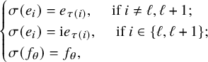 $$ \begin{align} \begin{cases} \sigma(e_i)=e_{\tau(i)}, \quad \text{ if } i\not= \ell, \ell+1; \\ \sigma(e_i)= \mathrm{i} e_{\tau(i)}, \quad \text{ if } i\in \{\ell, \ell+1\}; \\ \sigma(f_\theta)=f_\theta, \end{cases} \end{align} $$
where $\mathrm {i}$
is a square root of
$\mathrm {i}$
is a square root of $-1$
. One can check that
$-1$
. One can check that
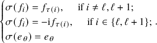 $$ \begin{align} \begin{cases} \sigma(f_i)= f_{\tau(i)}, \quad \text{ if } i\not= \ell, \ell+1; \\ \sigma(f_i)= -\mathrm{i} f_{\tau(i)}, \quad \text{ if } i\in \{\ell, \ell+1\}; \\ \sigma(e_\theta)=e_\theta \end{cases}\!\!\!\!\!. \end{align} $$
In fact, $\sigma = \tau \circ {\mathrm i}^{ h} $
, where
$\sigma = \tau \circ {\mathrm i}^{ h} $
, where $h\in \mathfrak {h}$
such that
$h\in \mathfrak {h}$
such that
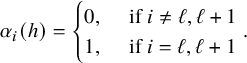 $$\begin{align*}\alpha_i(h)=\begin{cases} 0 , \quad \text{ if } i\not= \ell, \ell+1 \\ 1, \quad \text{ if } i=\ell, \ell+1 \end{cases}\!\!\!\!\!. \end{align*}$$
This automorphism induces a unique automorphism on G. We still call it $\sigma $
.
$\sigma $
.
We call these automorphisms on G or $\mathfrak {g}$
‘standard’, as the fixed point Lie subalgebra
$\mathfrak {g}$
‘standard’, as the fixed point Lie subalgebra $\mathfrak {g}^\sigma $
is the standard finite part of the associated twisted affine Lie algebra
$\mathfrak {g}^\sigma $
is the standard finite part of the associated twisted affine Lie algebra $\hat {L}(\mathfrak {g},\sigma )$
(cf. Section 3.1) in the sense of Kac [Reference KacKa, §6.3]. From
$\hat {L}(\mathfrak {g},\sigma )$
(cf. Section 3.1) in the sense of Kac [Reference KacKa, §6.3]. From $\sigma $
, we will construct a twisted affine Grassmannian and a line bundle of level one on it. There will be no level one line bundle on the twisted affine Grassmannian associated to
$\sigma $
, we will construct a twisted affine Grassmannian and a line bundle of level one on it. There will be no level one line bundle on the twisted affine Grassmannian associated to $\tau $
on G of type
$\tau $
on G of type $A_{2\ell }$
. Throughout this paper, we will only consider standard automorphisms.
$A_{2\ell }$
. Throughout this paper, we will only consider standard automorphisms.
The following table describe the fixed point Lie algebras for all standard automorphisms:
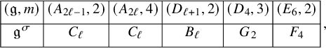
where by convention, $C_1$
is
$C_1$
is $A_1$
and
$A_1$
and $\ell \geq 3$
for
$\ell \geq 3$
for $D_{\ell +1}$
. When
$D_{\ell +1}$
. When $(\mathfrak {g}, m)\not =(A_{2\ell }, 4) $
, the fixed point Lie algebra
$(\mathfrak {g}, m)\not =(A_{2\ell }, 4) $
, the fixed point Lie algebra $\mathfrak {g}^\sigma $
is well known as listed in the above table. When
$\mathfrak {g}^\sigma $
is well known as listed in the above table. When $(\mathfrak {g}, m)=(A_{2\ell }, 4) $
, the fixed Lie algebra
$(\mathfrak {g}, m)=(A_{2\ell }, 4) $
, the fixed Lie algebra $\mathfrak {g}^\sigma $
is of type
$\mathfrak {g}^\sigma $
is of type $C_\ell $
, which can follow from the twisted Kac-Moody theory; cf. [Reference KacKa, §6.3, §8.4].
$C_\ell $
, which can follow from the twisted Kac-Moody theory; cf. [Reference KacKa, §6.3, §8.4].
Recall that we follow the Bourbaki labelling of the vertices of the Dynkin diagram. Set
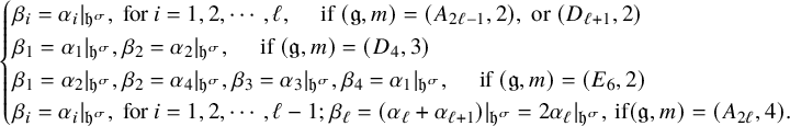 $$ \begin{align} \begin{cases} \beta_i= {\alpha_i} |_ {\mathfrak{h}^\sigma}, \text{ for } i=1,2,\cdots, \ell, \quad \text{ if } (\mathfrak{g}, m)=(A_{2\ell-1}, 2), \text{ or } (D_{\ell+1}, 2) \\ \beta_1=\alpha_1|_{\mathfrak{h}^\sigma}, \beta_2=\alpha_2|_{\mathfrak{h}^\sigma}, \quad \text{ if } (\mathfrak{g}, m)=(D_4, 3)\\ \beta_1=\alpha_2|_{\mathfrak{h}^\sigma}, \beta_2=\alpha_4|_{\mathfrak{h}^\sigma},\beta_3=\alpha_3|_{\mathfrak{h}^\sigma},\beta_4=\alpha_1|_{\mathfrak{h}^\sigma}, \quad \text{ if } (\mathfrak{g}, m)=(E_6, 2)\\ \beta_i= \alpha_i |_ {\mathfrak{h}^\sigma}, \text{ for } i=1,2,\cdots, \ell-1; \beta_\ell= (\alpha_\ell+\alpha_{\ell+1}) |_ {\mathfrak{h}^\sigma}=2\alpha_\ell|_{\mathfrak{h}^\sigma}, \, \text{if} (\mathfrak{g}, m)=(A_{2\ell}, 4). \end{cases} \end{align} $$
Let $I_\sigma $
be the set of all subscript indices of
$I_\sigma $
be the set of all subscript indices of $\beta _i$
. Then for each case, the set
$\beta _i$
. Then for each case, the set $\{\,\beta _j \,|\, j\in I_\sigma \, \}$
gives rise to the set of simple roots of
$\{\,\beta _j \,|\, j\in I_\sigma \, \}$
gives rise to the set of simple roots of $\mathfrak {g}^\sigma $
. One can see easily that this labelling will coincide with Bourbaki labelling for nonsimply-laced types Dynkin diagrams.
$\mathfrak {g}^\sigma $
. One can see easily that this labelling will coincide with Bourbaki labelling for nonsimply-laced types Dynkin diagrams.
We now define a map $\eta : I\to I_\sigma $
. When
$\eta : I\to I_\sigma $
. When $(\mathfrak {g}, m)\not = (A_{2\ell }, 4)$
,
$(\mathfrak {g}, m)\not = (A_{2\ell }, 4)$
, $\eta $
is defined such that
$\eta $
is defined such that $\beta _{\eta (i) }= \alpha _i|_{\mathfrak {h}^\sigma }$
for any
$\beta _{\eta (i) }= \alpha _i|_{\mathfrak {h}^\sigma }$
for any $i\in I$
. When
$i\in I$
. When $(\mathfrak {g}, m)= (A_{2\ell }, 4)$
, set
$(\mathfrak {g}, m)= (A_{2\ell }, 4)$
, set
 $$\begin{align*}\eta(i)=\eta(2\ell+1-i)=i, \text{ for any } 1\leq i\leq \ell. \end{align*}$$
Let $\{ \,\check {\beta }_j \,|\, j\in I_\sigma \}$
be the set of simple coroots of
$\{ \,\check {\beta }_j \,|\, j\in I_\sigma \}$
be the set of simple coroots of $\mathfrak {g}^\sigma $
. We can describe
$\mathfrak {g}^\sigma $
. We can describe $\check {\beta }_j $
as follows:
$\check {\beta }_j $
as follows:
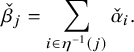 $$ \begin{align} \check{\beta}_j= \sum_{i\in \eta^{-1}(j) } \check{\alpha}_{ i }. \end{align} $$
The description of $\check {\beta }_j $
also appears in [Reference HainesHa, Section 3] in a slightly different setting.
$\check {\beta }_j $
also appears in [Reference HainesHa, Section 3] in a slightly different setting.
Let $\{\, \lambda _j \,|\, j\in I_\sigma \,\}$
be the set of fundamental weights of
$\{\, \lambda _j \,|\, j\in I_\sigma \,\}$
be the set of fundamental weights of $\mathfrak {g}^\sigma $
, and let
$\mathfrak {g}^\sigma $
, and let $\{\, \check {\lambda }_j \,|\, j\in I_\sigma \,\}$
be the set of fundamental coweights of
$\{\, \check {\lambda }_j \,|\, j\in I_\sigma \,\}$
be the set of fundamental coweights of $\mathfrak {g}^\sigma $
. The fundamental weights can be described as follows:
$\mathfrak {g}^\sigma $
. The fundamental weights can be described as follows:
 $$ \begin{align} \lambda_j= \omega_i|_{\mathfrak{h}^\sigma}, \quad \text{ for some } i \text{ with } \eta(i)=j. \end{align} $$
In the case of fundamental coweights, we need to describe them separately. When $(\mathfrak {g}, m)\not = (A_{2\ell }, 4)$
,
$(\mathfrak {g}, m)\not = (A_{2\ell }, 4)$
,
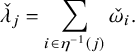 $$ \begin{align} \check{\lambda}_j=\sum_{i\in \eta^{-1}(j)} \check{\omega}_i. \end{align} $$
When $(\mathfrak {g},m)=(A_{2\ell }, 4)$
, we have
$(\mathfrak {g},m)=(A_{2\ell }, 4)$
, we have
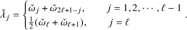 $$ \begin{align} \check{\lambda}_j= \begin{cases} \check{\omega}_j+\check{\omega}_{2\ell+1-j}, \quad \quad j=1,2,\cdots, \ell-1 \\ \frac{1}{2}(\check{\omega}_\ell + \check{\omega}_{\ell+1} ), \quad \quad j=\ell \end{cases}\!\!\!\!\!. \end{align} $$
2.2 Affine Grassmannian of special parahoric group schemes
Let $\mathcal {K}$
denote the field of formal Laurent series in t with coefficients in
$\mathcal {K}$
denote the field of formal Laurent series in t with coefficients in $\mathbb {C}$
. Let
$\mathbb {C}$
. Let $\mathcal {O} $
denote the ring of formal power series in t with coefficients in
$\mathcal {O} $
denote the ring of formal power series in t with coefficients in $\mathbb {C}$
. By abuse of notation, we still use
$\mathbb {C}$
. By abuse of notation, we still use $\sigma $
to denote the automorphism of order m on
$\sigma $
to denote the automorphism of order m on $\mathcal {K}$
and
$\mathcal {K}$
and $\mathcal {O}$
such that
$\mathcal {O}$
such that $\sigma $
acts on
$\sigma $
acts on $\mathbb {C}$
trivially, and
$\mathbb {C}$
trivially, and $\sigma (t)=\epsilon ^{-1} t $
, where
$\sigma (t)=\epsilon ^{-1} t $
, where $\epsilon =e^{\frac {2\pi \mathrm {i}}{m}}$
. Set
$\epsilon =e^{\frac {2\pi \mathrm {i}}{m}}$
. Set $\bar { \mathcal {K} } =\mathcal {K}^\sigma $
and
$\bar { \mathcal {K} } =\mathcal {K}^\sigma $
and $\bar { \mathcal {O} } =\mathcal {O}^\sigma $
. Then
$\bar { \mathcal {O} } =\mathcal {O}^\sigma $
. Then $\bar { \mathcal {K} } ={\mathbb {C}}((\bar {t})) $
and
$\bar { \mathcal {K} } ={\mathbb {C}}((\bar {t})) $
and $\bar { \mathcal {O} } ={\mathbb {C}}[[\bar {t}]]$
, where
$\bar { \mathcal {O} } ={\mathbb {C}}[[\bar {t}]]$
, where $\bar {t}=t^m$
.
$\bar {t}=t^m$
.
Let ${\mathscr {G}}$
be the smooth group scheme
${\mathscr {G}}$
be the smooth group scheme $\mathrm {Res}_{\mathcal {O}/\bar {\mathcal {O}} } (G_{\mathcal {O}})^\sigma $
over
$\mathrm {Res}_{\mathcal {O}/\bar {\mathcal {O}} } (G_{\mathcal {O}})^\sigma $
over $\bar { \mathcal {O} } $
, which represents the following group functor
$\bar { \mathcal {O} } $
, which represents the following group functor
 $$\begin{align*}R\mapsto G(\mathcal{O}\otimes_{\bar{ \mathcal{O} } } R)^\sigma , \quad \text{ for any } \bar{ \mathcal{O} } -\text{algebra } R, \end{align*}$$
where the $G(\mathcal {O}\otimes _{\bar { \mathcal {O} } } R)$
denotes the group of
$G(\mathcal {O}\otimes _{\bar { \mathcal {O} } } R)$
denotes the group of $\sigma $
-equivariant morphisms from
$\sigma $
-equivariant morphisms from $\mathrm {Spec }\,( \mathcal {O}\otimes _{\bar {\mathcal {O}}} R)$
to G, where
$\mathrm {Spec }\,( \mathcal {O}\otimes _{\bar {\mathcal {O}}} R)$
to G, where $\sigma $
acts on
$\sigma $
acts on $\mathcal {O}$
as above and acts on G as a standard automorphism defined in Section 2.1. Then,
$\mathcal {O}$
as above and acts on G as a standard automorphism defined in Section 2.1. Then, ${\mathscr {G}}$
is a special parahoric group scheme in the sense of Bruhat-Tits, as we choose
${\mathscr {G}}$
is a special parahoric group scheme in the sense of Bruhat-Tits, as we choose $\sigma $
to be standard. In fact, up to isomorphism, this construction exhausts all special parahoric subgroups in
$\sigma $
to be standard. In fact, up to isomorphism, this construction exhausts all special parahoric subgroups in ${\mathscr {G}}(\mathcal {K})$
when
${\mathscr {G}}(\mathcal {K})$
when ${\mathscr {G}}$
is not of type
${\mathscr {G}}$
is not of type $A_{2\ell }^{(2)}$
, and special but not absolutely special for
$A_{2\ell }^{(2)}$
, and special but not absolutely special for $A_{2\ell }^{(2)}$
in the sense of [Reference Haines and RicharzHR, §5], as in this case the special fiber of
$A_{2\ell }^{(2)}$
in the sense of [Reference Haines and RicharzHR, §5], as in this case the special fiber of ${\mathscr {G}}$
has a quotient isomorphic to
${\mathscr {G}}$
has a quotient isomorphic to $\mathrm {Sp}_{2\ell }$
.
$\mathrm {Sp}_{2\ell }$
.
Remark 2.1. When G is of type $A_{2\ell }$
, the parahoric group scheme
$A_{2\ell }$
, the parahoric group scheme ${\mathscr {G}}=\mathrm { Res}_{\mathcal {O}/\bar {\mathcal {O}} } (G_{\mathcal {O}})^\tau $
is absolutely special of type
${\mathscr {G}}=\mathrm { Res}_{\mathcal {O}/\bar {\mathcal {O}} } (G_{\mathcal {O}})^\tau $
is absolutely special of type $A_{2\ell }^{(2)}$
, where
$A_{2\ell }^{(2)}$
, where $\tau $
acts on G by a nontrivial diagram automorphism and acts on
$\tau $
acts on G by a nontrivial diagram automorphism and acts on $\mathcal {O}$
by
$\mathcal {O}$
by $t\mapsto -t$
. But we will not consider this case, except in Remark 4.12.
$t\mapsto -t$
. But we will not consider this case, except in Remark 4.12.
We can similarly define the smooth group scheme ${\mathscr {T}}:=\mathrm {Res}_{\mathcal {O}/\bar {\mathcal {O}} } (T_{\mathcal {O}})^\sigma $
, which has connected fibers (cf. [Reference Bruhat and TitsBrT, Lemma 4.4.16, Lemma 4.4.8]). Note that, for general almost simple algebraic group G, we can still define
${\mathscr {T}}:=\mathrm {Res}_{\mathcal {O}/\bar {\mathcal {O}} } (T_{\mathcal {O}})^\sigma $
, which has connected fibers (cf. [Reference Bruhat and TitsBrT, Lemma 4.4.16, Lemma 4.4.8]). Note that, for general almost simple algebraic group G, we can still define ${\mathscr {G}}$
and
${\mathscr {G}}$
and ${\mathscr {T}}$
, but we need to take the neutral components of
${\mathscr {T}}$
, but we need to take the neutral components of $\mathrm {Res}_{\mathcal {O}/\bar {\mathcal {O}} } (G_{\mathcal {O}})^\sigma $
and
$\mathrm {Res}_{\mathcal {O}/\bar {\mathcal {O}} } (G_{\mathcal {O}})^\sigma $
and $\mathrm { Res}_{\mathcal {O}/\bar {\mathcal {O}} } (T_{\mathcal {O}})^\sigma $
, respectively. For convenience, throughout this paper, we only work with G being adjoint or simply-connected.
$\mathrm { Res}_{\mathcal {O}/\bar {\mathcal {O}} } (T_{\mathcal {O}})^\sigma $
, respectively. For convenience, throughout this paper, we only work with G being adjoint or simply-connected.
Let $L^+ {\mathscr {G}}$
denote the jet group and
$L^+ {\mathscr {G}}$
denote the jet group and $L{\mathscr {G}}$
be the loop group of
$L{\mathscr {G}}$
be the loop group of ${\mathscr {G}}$
over
${\mathscr {G}}$
over $\mathbb {C}$
; that is, for all
$\mathbb {C}$
; that is, for all $\mathbb {C}$
-algebras R, we set
$\mathbb {C}$
-algebras R, we set $L^+{\mathscr {G}}(R)={\mathscr {G}}( R[[t]])$
and
$L^+{\mathscr {G}}(R)={\mathscr {G}}( R[[t]])$
and $L{\mathscr {G}}(R)= {\mathscr {G}}(R((t)))$
. We denote by
$L{\mathscr {G}}(R)= {\mathscr {G}}(R((t)))$
. We denote by $\operatorname {\mathrm {\mathtt {Gr}}}_{\mathscr {G}}$
the affine Grassmannian of
$\operatorname {\mathrm {\mathtt {Gr}}}_{\mathscr {G}}$
the affine Grassmannian of ${\mathscr {G}}$
, which is defined as the fppf quotient
${\mathscr {G}}$
, which is defined as the fppf quotient $L{\mathscr {G}}/L^+{\mathscr {G}}$
. In particular, we have
$L{\mathscr {G}}/L^+{\mathscr {G}}$
. In particular, we have
 $$\begin{align*}\operatorname{\mathrm{\mathtt{Gr}}}_{\mathscr{G}}({\mathbb{C}})= G(\mathcal{K})^\sigma/ G(\mathcal{O} ) ^\sigma. \end{align*}$$
It is known that $\operatorname {\mathrm {\mathtt {Gr}}}_{\mathscr {G}}$
is a projective ind-variety; cf. [Reference Pappas and RapoportPR, Theorem 1.4]. Following [Reference Pappas and RapoportPR, Reference ZhuZh2], we will call it a twisted affine Grassmannian of
$\operatorname {\mathrm {\mathtt {Gr}}}_{\mathscr {G}}$
is a projective ind-variety; cf. [Reference Pappas and RapoportPR, Theorem 1.4]. Following [Reference Pappas and RapoportPR, Reference ZhuZh2], we will call it a twisted affine Grassmannian of ${\mathscr {G}}$
. We can also attach the twisted affine Grassmannian
${\mathscr {G}}$
. We can also attach the twisted affine Grassmannian $\operatorname {\mathrm {\mathtt {Gr}}}_{ {\mathscr {T}} }:=L {\mathscr {T}}/L^+ {\mathscr {T}}$
of
$\operatorname {\mathrm {\mathtt {Gr}}}_{ {\mathscr {T}} }:=L {\mathscr {T}}/L^+ {\mathscr {T}}$
of ${\mathscr {T}}$
. This is a highly non-reduced ind-scheme. Moreover,
${\mathscr {T}}$
. This is a highly non-reduced ind-scheme. Moreover,
 $$\begin{align*}\operatorname{\mathrm{\mathtt{Gr}}}_{ {\mathscr{T}} }({\mathbb{C}})= T(\mathcal{K})^\sigma/T(\mathcal{O})^\sigma. \end{align*}$$
For any $\lambda \in X_*(T)$
, we can naturally attach an element
$\lambda \in X_*(T)$
, we can naturally attach an element $t^\lambda \in T(\mathcal {K})$
. We now define the norm
$t^\lambda \in T(\mathcal {K})$
. We now define the norm $n^\lambda \in T(\mathcal {K} )^\sigma $
of
$n^\lambda \in T(\mathcal {K} )^\sigma $
of $t^\lambda $
,
$t^\lambda $
,
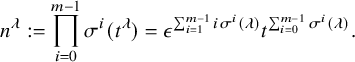 $$ \begin{align} n^\lambda:= \prod_{i=0}^{m-1} \sigma^i(t^\lambda)=\epsilon^{\sum_{i=1}^{m-1} i \sigma^i(\lambda) } t^{\sum_{i=0}^{m-1} \sigma^i(\lambda)}. \end{align} $$
There exists a natural bijection
 $$ \begin{align} T(\mathcal{K})^\sigma/T(\mathcal{O})^\sigma \simeq X_*(T)_\sigma , \end{align} $$
where $X_*(T)_\sigma $
denotes the set of
$X_*(T)_\sigma $
denotes the set of $\sigma $
-coinvariants in
$\sigma $
-coinvariants in $X_*(T)$
. Any
$X_*(T)$
. Any $\bar {\lambda }\in X_*(T)_\sigma $
corresponds to the coset
$\bar {\lambda }\in X_*(T)_\sigma $
corresponds to the coset $n^\lambda T( \mathcal {O})^\sigma $
, where
$n^\lambda T( \mathcal {O})^\sigma $
, where $\lambda $
is a representative of
$\lambda $
is a representative of $\bar {\lambda }$
. By Theorem [Reference Pappas and RapoportPR, Theorem 0.1], the components of
$\bar {\lambda }$
. By Theorem [Reference Pappas and RapoportPR, Theorem 0.1], the components of $\operatorname {\mathrm {\mathtt {Gr}}}_{{\mathscr {G}} }$
can be parametrized by elements in
$\operatorname {\mathrm {\mathtt {Gr}}}_{{\mathscr {G}} }$
can be parametrized by elements in $\pi _1(G)_\sigma $
, where
$\pi _1(G)_\sigma $
, where $\pi _1(G)\simeq X_*(T)/\check {Q}$
, and
$\pi _1(G)\simeq X_*(T)/\check {Q}$
, and $(X_*(T)/\check {Q})_\sigma $
is the the set of coinvariants of
$(X_*(T)/\check {Q})_\sigma $
is the the set of coinvariants of $\sigma $
in
$\sigma $
in $X_*(T)/\check {Q}$
.
$X_*(T)/\check {Q}$
.
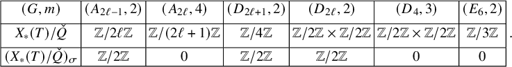
When G is of adjoint type, we describe $(X_*(T)/\check {Q})_\sigma $
in the following table.
$(X_*(T)/\check {Q})_\sigma $
in the following table.
2.3 Twisted affine Schubert varieties
Let $e_0$
be the base point in
$e_0$
be the base point in $\operatorname {\mathrm {\mathtt {Gr}}}_{\mathscr {G}}({\mathbb {C}})$
. For any
$\operatorname {\mathrm {\mathtt {Gr}}}_{\mathscr {G}}({\mathbb {C}})$
. For any $\bar {\lambda }\in X_*(T) _\sigma $
, let
$\bar {\lambda }\in X_*(T) _\sigma $
, let $e_{\bar {\lambda }}$
denote the point
$e_{\bar {\lambda }}$
denote the point $n^\lambda e_0 \in \operatorname {\mathrm {\mathtt {Gr}}}_{{\mathscr {G}} }( {\mathbb {C}})$
. The point
$n^\lambda e_0 \in \operatorname {\mathrm {\mathtt {Gr}}}_{{\mathscr {G}} }( {\mathbb {C}})$
. The point $e_{\bar {\lambda }}$
only depends on
$e_{\bar {\lambda }}$
only depends on $\bar {\lambda }\in X_*(T)_\sigma $
. Let
$\bar {\lambda }\in X_*(T)_\sigma $
. Let $X_*(T)^+_\sigma $
denote the set of images of
$X_*(T)^+_\sigma $
denote the set of images of $X_*(T)^+$
in
$X_*(T)^+$
in $X_*(T)_\sigma $
via the projection
$X_*(T)_\sigma $
via the projection $X_*(T)\to X_*(T)_\sigma $
. Then, we have the following Cartan decomposition for
$X_*(T)\to X_*(T)_\sigma $
. Then, we have the following Cartan decomposition for $\operatorname {\mathrm {\mathtt {Gr}}}_{\mathscr {G}}$
(cf. [Reference RicharzRi1, Proposition 2.8]):
$\operatorname {\mathrm {\mathtt {Gr}}}_{\mathscr {G}}$
(cf. [Reference RicharzRi1, Proposition 2.8]):
 $$ \begin{align} \operatorname{\mathrm{\mathtt{Gr}}}_{\mathscr{G}}({\mathbb{C}})= \bigsqcup_{\bar{ \lambda} \in X_*(T)^+_\sigma } \operatorname{\mathrm{\mathtt{Gr}}}_{\mathscr{G}}^{\bar{\lambda}} , \end{align} $$
where $\operatorname {\mathrm {\mathtt {Gr}}}_{\mathscr {G}}^{\bar {\lambda }}:= G(\mathcal {O})^\sigma e_{\bar {\lambda }} $
. The Schubert variety
$\operatorname {\mathrm {\mathtt {Gr}}}_{\mathscr {G}}^{\bar {\lambda }}:= G(\mathcal {O})^\sigma e_{\bar {\lambda }} $
. The Schubert variety $\overline { \operatorname {\mathrm {\mathtt {Gr}}} }_{\mathscr {G}}^{\bar {\lambda }} $
is defined to be the reduced closure of
$\overline { \operatorname {\mathrm {\mathtt {Gr}}} }_{\mathscr {G}}^{\bar {\lambda }} $
is defined to be the reduced closure of $\operatorname {\mathrm {\mathtt {Gr}}}_{\mathscr {G}}^{\bar {\lambda }}$
in
$\operatorname {\mathrm {\mathtt {Gr}}}_{\mathscr {G}}^{\bar {\lambda }}$
in $\operatorname {\mathrm {\mathtt {Gr}}}_{\mathscr {G}}$
. Moreover,
$\operatorname {\mathrm {\mathtt {Gr}}}_{\mathscr {G}}$
. Moreover,
 $$\begin{align*}\dim \overline{ \operatorname{\mathrm{\mathtt{Gr}}} }_{\mathscr{G}}^{\bar{\lambda}} =2\langle \lambda, \rho \rangle ,\end{align*}$$
where $\rho $
is the sum of all fundamental weights of
$\rho $
is the sum of all fundamental weights of $\mathfrak {g}$
. It is easy to see that the dimension is independent of the choice of
$\mathfrak {g}$
. It is easy to see that the dimension is independent of the choice of $\lambda $
.
$\lambda $
.
For any $\bar {\lambda },\bar {\mu }\in X_*(T)^+_\sigma $
, we write
$\bar {\lambda },\bar {\mu }\in X_*(T)^+_\sigma $
, we write $\bar {\mu }\preceq \bar {\lambda }$
if
$\bar {\mu }\preceq \bar {\lambda }$
if $\operatorname {\mathrm {\mathtt {Gr}}}_{\mathscr {G}}^{\bar {\mu }} \subseteq \overline { \operatorname {\mathrm {\mathtt {Gr}}} }_{\mathscr {G}}^{\bar {\lambda }} $
. For any
$\operatorname {\mathrm {\mathtt {Gr}}}_{\mathscr {G}}^{\bar {\mu }} \subseteq \overline { \operatorname {\mathrm {\mathtt {Gr}}} }_{\mathscr {G}}^{\bar {\lambda }} $
. For any $i\in I$
, let
$i\in I$
, let $\overline {\check {\alpha }}_i$
denote the image of
$\overline {\check {\alpha }}_i$
denote the image of $\check {\alpha }_i$
in
$\check {\alpha }_i$
in $X_*(T)_\sigma $
. For any
$X_*(T)_\sigma $
. For any $j\in I_\sigma $
, set
$j\in I_\sigma $
, set
 $$ \begin{align} \gamma_j =\overline{\check{\alpha}}_i, \quad \text{ if } j=\eta(i). \end{align} $$
It is clear that $\gamma _j $
is well defined.
$\gamma _j $
is well defined.
The following lemma follows from [Reference RicharzRi1, Corollary 2.10].
Lemma 2.2. $\bar {\mu }\preceq \bar {\lambda }$
if and only if
$\bar {\mu }\preceq \bar {\lambda }$
if and only if $\bar {\lambda }-\bar {\mu }$
is a nonnegative integral linear combination of
$\bar {\lambda }-\bar {\mu }$
is a nonnegative integral linear combination of $\{ \,\gamma _j \,|\, j\in I_\sigma \,\}$
.
$\{ \,\gamma _j \,|\, j\in I_\sigma \,\}$
.
By the ramified geometric correspondence [Reference ZhuZh3, §1], the set $X_*(T)_\sigma $
can be realized as the weight lattice of the reductive group
$X_*(T)_\sigma $
can be realized as the weight lattice of the reductive group $H:=(\check {G})^\tau $
, where
$H:=(\check {G})^\tau $
, where $\check {G}$
is the Langlands dual group of G and
$\check {G}$
is the Langlands dual group of G and $\tau $
is a diagram automorphism on
$\tau $
is a diagram automorphism on $\check {G}$
corresponding to the one on G, and
$\check {G}$
corresponding to the one on G, and $\{ \,\gamma _j \,|\, j\in I_\sigma \,\}$
is the set of simple roots for H. Moreover,
$\{ \,\gamma _j \,|\, j\in I_\sigma \,\}$
is the set of simple roots for H. Moreover, $X_*(T)^+_\sigma $
is the set of dominant weights of H, and the partial order
$X_*(T)^+_\sigma $
is the set of dominant weights of H, and the partial order $\preceq $
is exactly the standard partial order for dominant weights of H.
$\preceq $
is exactly the standard partial order for dominant weights of H.
We now assume G is of adjoint type. From the perspective of the geometric Satake, we can determine the minimal elements in $ X_*(T)^+_\sigma $
, in other words the minimal Schubert variety in each connected component of
$ X_*(T)^+_\sigma $
, in other words the minimal Schubert variety in each connected component of $\operatorname {\mathrm {\mathtt {Gr}}}_{{\mathscr {G}} }$
. From the table (2.11), we see that when
$\operatorname {\mathrm {\mathtt {Gr}}}_{{\mathscr {G}} }$
. From the table (2.11), we see that when $(G, m)=(A_{2\ell -1}, 2 )$
,
$(G, m)=(A_{2\ell -1}, 2 )$
, $\operatorname {\mathrm {\mathtt {Gr}}}_{{\mathscr {G}} }$
has two components, where
$\operatorname {\mathrm {\mathtt {Gr}}}_{{\mathscr {G}} }$
has two components, where $\operatorname {\mathrm {\mathtt {Gr}}}_{{\mathscr {G}} }^{ \overline { \check {\omega } }_1 } $
is the minimal Schubert variety in the non-neutral component, since
$\operatorname {\mathrm {\mathtt {Gr}}}_{{\mathscr {G}} }^{ \overline { \check {\omega } }_1 } $
is the minimal Schubert variety in the non-neutral component, since $ \overline { \check {\omega } }_1$
gives the minuscule dominant weight of
$ \overline { \check {\omega } }_1$
gives the minuscule dominant weight of $H\simeq \mathrm {Sp}_{2\ell }$
. When
$H\simeq \mathrm {Sp}_{2\ell }$
. When $(G, m)=(D_{\ell +1}, 2 )$
,
$(G, m)=(D_{\ell +1}, 2 )$
, $\operatorname {\mathrm {\mathtt {Gr}}}_{{\mathscr {G}} }$
also has two components and
$\operatorname {\mathrm {\mathtt {Gr}}}_{{\mathscr {G}} }$
also has two components and $\operatorname {\mathrm {\mathtt {Gr}}}_{{\mathscr {G}} }^{ \overline { \check {\omega } }_\ell } $
is the minimal Schubert variety in the non-neutral component, since
$\operatorname {\mathrm {\mathtt {Gr}}}_{{\mathscr {G}} }^{ \overline { \check {\omega } }_\ell } $
is the minimal Schubert variety in the non-neutral component, since $\overline { \check {\omega } }_\ell $
is the minuscule dominant weight of
$\overline { \check {\omega } }_\ell $
is the minuscule dominant weight of $H\simeq \mathrm {Spin}_{2\ell +1}$
. Otherwise,
$H\simeq \mathrm {Spin}_{2\ell +1}$
. Otherwise, $\operatorname {\mathrm {\mathtt {Gr}}}_{{\mathscr {G}} }$
has only one component. In fact, when
$\operatorname {\mathrm {\mathtt {Gr}}}_{{\mathscr {G}} }$
has only one component. In fact, when $(G, m)=(A_{2\ell }, 4)$
,
$(G, m)=(A_{2\ell }, 4)$
, $H\simeq \mathrm {SO}_{2\ell +1}$
, in which case the lattice
$H\simeq \mathrm {SO}_{2\ell +1}$
, in which case the lattice $X_*(T)_\sigma $
concides with the root lattice of H.
$X_*(T)_\sigma $
concides with the root lattice of H.
Let S denote the following set:
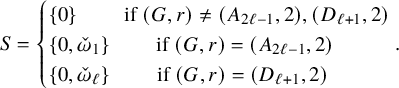 $$ \begin{align} S=\begin{cases}\{ 0\} \quad \quad \text{ if } (G,r)\not= (A_{2\ell-1}, 2 ), (D_{\ell+1}, 2 ) \\ \{ 0, \check{\omega}_1 \} \quad \quad \text{ if } (G,r)= (A_{2\ell-1}, 2 ) \\ \{0, \check{\omega}_\ell \} \quad\quad \text{ if } (G,r)= (D_{\ell+1}, 2 ) \\ \end{cases}\!\!\!\!\!. \end{align} $$
For any $\kappa \in S$
, let
$\kappa \in S$
, let $\operatorname {\mathrm {\mathtt {Gr}}}_{{\mathscr {G}} , \kappa }$
be the component of
$\operatorname {\mathrm {\mathtt {Gr}}}_{{\mathscr {G}} , \kappa }$
be the component of $\operatorname {\mathrm {\mathtt {Gr}}}_{\mathscr {G}} $
containing the Schubert variety
$\operatorname {\mathrm {\mathtt {Gr}}}_{\mathscr {G}} $
containing the Schubert variety $\operatorname {\mathrm {\mathtt {Gr}}}_{\mathscr {G}} ^{ \bar {\kappa } }$
, or equivalently containing the point
$\operatorname {\mathrm {\mathtt {Gr}}}_{\mathscr {G}} ^{ \bar {\kappa } }$
, or equivalently containing the point $e_{\bar {\kappa }}$
. Then,
$e_{\bar {\kappa }}$
. Then,
 $$\begin{align*}\operatorname{\mathrm{\mathtt{Gr}}}_{\mathscr{G}} = \sqcup_{\kappa\in S} \operatorname{\mathrm{\mathtt{Gr}}}_{{\mathscr{G}} , \kappa}. \end{align*}$$
2.4 Global affine Grassmannian of parahoric Bruhat-Tits group schemes
Let C be a complex projective line $\mathbb {P}^1$
with a coordinate t, and with the action of
$\mathbb {P}^1$
with a coordinate t, and with the action of $\sigma $
such that
$\sigma $
such that $t\mapsto \epsilon t$
. Let
$t\mapsto \epsilon t$
. Let $\bar {C}$
be the quotient curve
$\bar {C}$
be the quotient curve $C/\sigma $
, and let
$C/\sigma $
, and let $\pi : C\to \bar {C}$
be the projection map. Then
$\pi : C\to \bar {C}$
be the projection map. Then $\bar {C}$
is also isomorphic to
$\bar {C}$
is also isomorphic to $\mathbb {P}^1$
. Let
$\mathbb {P}^1$
. Let $\mathcal {G}=\operatorname {{\mathrm {Res}}}_{C/\bar {C}}(G \times C)^{\sigma }$
be the group scheme over
$\mathcal {G}=\operatorname {{\mathrm {Res}}}_{C/\bar {C}}(G \times C)^{\sigma }$
be the group scheme over $\bar {C}$
, which is the
$\bar {C}$
, which is the $\sigma $
-fixed point subgroup scheme of the Weil restriction
$\sigma $
-fixed point subgroup scheme of the Weil restriction $\operatorname {{\mathrm {Res}}}_{C/\bar {C}}(G \times C)$
of the constant group scheme
$\operatorname {{\mathrm {Res}}}_{C/\bar {C}}(G \times C)$
of the constant group scheme $G\times C$
from C to
$G\times C$
from C to $\bar {C}$
. Then,
$\bar {C}$
. Then, $\mathcal {G}$
is a parahoric Bruhat-Tits group scheme over
$\mathcal {G}$
is a parahoric Bruhat-Tits group scheme over $\bar {C}$
in the sense of Heinloth [Reference HeinlothHe, §1]. Let o (resp.
$\bar {C}$
in the sense of Heinloth [Reference HeinlothHe, §1]. Let o (resp. $\bar {o}$
) be the origin of C (resp.
$\bar {o}$
) be the origin of C (resp. $\bar {C}$
), and let
$\bar {C}$
), and let $\infty $
(resp.
$\infty $
(resp. $\bar {\infty }$
) be the infinite point in C (resp.
$\bar {\infty }$
) be the infinite point in C (resp. $\bar {C}$
).
$\bar {C}$
).
The group scheme $\mathcal {G}$
has the following properties:
$\mathcal {G}$
has the following properties:
-
1. For any
$y\in \bar {C}$
, if
$y\not =\bar {o}, \bar {\infty }$
, the fiber
$\mathcal {G}_{|_y}$
over y is isomorphic to G; the restriction
$\mathcal {G}_y$
to the formal disc
$\mathbb {D}_y$
around y is isomorphic to the constant group scheme
$G_{ \mathbb {D}_y}$
over
$\mathbb {D}_y$
. -
2. When
$y=\bar {o}$
or
$\bar {\infty }$
in
$\bar {C}$
,
$\mathcal {G}_{|_y}$
has a reductive quotient
$G^\sigma $
; the restriction
$\mathcal {G}_y$
to
$\mathbb {D}_y$
is isomorphic to the parahoric group scheme
${\mathscr {G}}$
.


Similarly, we can define the parahoric Bruhat-Tits group scheme $\mathcal {T}:= \operatorname {{\mathrm {Res}}}_{C/\bar {C}}(T \times C)^{\sigma }$
.
$\mathcal {T}:= \operatorname {{\mathrm {Res}}}_{C/\bar {C}}(T \times C)^{\sigma }$
.
Given an R-point $p \in C(R)$
, we denote by
$p \in C(R)$
, we denote by $\Gamma _p\subset C_R$
the graph of p where
$\Gamma _p\subset C_R$
the graph of p where $C_R:=C\times \mathrm { Spec} (R)$
, and denote by
$C_R:=C\times \mathrm { Spec} (R)$
, and denote by $\hat {\Gamma }_p$
the formal completion of
$\hat {\Gamma }_p$
the formal completion of $C_R$
along
$C_R$
along $\Gamma _p$
, and let
$\Gamma _p$
, and let $\hat {\Gamma }^\times _{p} $
be the punctured formal completion along
$\hat {\Gamma }^\times _{p} $
be the punctured formal completion along $\Gamma _p$
. Let
$\Gamma _p$
. Let $\bar {p}$
be the image of p in
$\bar {p}$
be the image of p in $\bar {C}$
. We similarly define
$\bar {C}$
. We similarly define $\bar {C}_R$
,
$\bar {C}_R$
, $\Gamma _{\bar {p}}$
,
$\Gamma _{\bar {p}}$
, $\hat {\Gamma }_{\bar {p}}$
and
$\hat {\Gamma }_{\bar {p}}$
and $\hat {\Gamma }_{\bar {p}}^\times $
.
$\hat {\Gamma }_{\bar {p}}^\times $
.
For any $\mathbb {C}$
-algebra R, we define
$\mathbb {C}$
-algebra R, we define
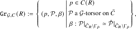 $$ \begin{align} \operatorname{\mathrm{\mathtt{Gr}}}_{\mathcal{G}, C}(R):= \left. \left\{ \, (p, \mathcal{P}, \beta) \, \middle | \, \begin{aligned}[m] & \, p \in C(R) \\ & \mathcal{P} \text{ a } \mathcal{G}\text{-torsor on } \bar{C} \\ & \, \beta: \mathcal{P}|_{\bar{C}_R \setminus {\Gamma}_{\bar{p}}} \simeq \mathring{\mathcal{P}}|_{\bar{C}_R \setminus \Gamma_{\bar{p}} }\\ \end{aligned} \right\} \right. , \end{align} $$
where $\mathring {\mathcal {P}}$
is the trivial
$\mathring {\mathcal {P}}$
is the trivial $\mathcal {G}$
-bundle.
$\mathcal {G}$
-bundle.
The functor $\operatorname {\mathrm {\mathtt {Gr}}}_{\mathcal {G}, C}$
is represented by an ind-scheme which is ind-proper over C. We call it the global affine Grassmannian
$\operatorname {\mathrm {\mathtt {Gr}}}_{\mathcal {G}, C}$
is represented by an ind-scheme which is ind-proper over C. We call it the global affine Grassmannian $\operatorname {\mathrm {\mathtt {Gr}}}_{\mathcal {G},C}$
of
$\operatorname {\mathrm {\mathtt {Gr}}}_{\mathcal {G},C}$
of $\mathcal {G}$
over C.
$\mathcal {G}$
over C.
For any $p\not =o,\infty \in C$
, the fiber
$p\not =o,\infty \in C$
, the fiber $\operatorname {\mathrm {\mathtt {Gr}}}_{\mathcal {G}, p}:=\operatorname {\mathrm {\mathtt {Gr}}}_{\mathcal {G}, C}|_p$
is isomorphic to the usual affine Grassmannian
$\operatorname {\mathrm {\mathtt {Gr}}}_{\mathcal {G}, p}:=\operatorname {\mathrm {\mathtt {Gr}}}_{\mathcal {G}, C}|_p$
is isomorphic to the usual affine Grassmannian $\operatorname {\mathrm {\mathtt {Gr}}}_G$
, and the fiber
$\operatorname {\mathrm {\mathtt {Gr}}}_G$
, and the fiber $\operatorname {\mathrm {\mathtt {Gr}}}_{\mathcal {G}, p}$
over
$\operatorname {\mathrm {\mathtt {Gr}}}_{\mathcal {G}, p}$
over $p=o,\infty $
is isomorphic to the twisted affine Grassmannian
$p=o,\infty $
is isomorphic to the twisted affine Grassmannian $\operatorname {\mathrm {\mathtt {Gr}}}_{\mathscr {G}}$
of the parahoric group scheme
$\operatorname {\mathrm {\mathtt {Gr}}}_{\mathscr {G}}$
of the parahoric group scheme ${\mathscr {G}}$
.
${\mathscr {G}}$
.
Remark 2.3. One can define the global affine Grassmannian $\operatorname {\mathrm {\mathtt {Gr}}}_{\mathcal {G}}$
over
$\operatorname {\mathrm {\mathtt {Gr}}}_{\mathcal {G}}$
over $\bar {C}$
; see [Reference ZhuZh2, Section 3.1]. The global affine Grassmannian defined above is actually the base change of
$\bar {C}$
; see [Reference ZhuZh2, Section 3.1]. The global affine Grassmannian defined above is actually the base change of $\operatorname {\mathrm {\mathtt {Gr}}}_{\mathcal {G}}$
along
$\operatorname {\mathrm {\mathtt {Gr}}}_{\mathcal {G}}$
along $\pi : C\to \bar {C}$
.
$\pi : C\to \bar {C}$
.
We can also define the jet group scheme $L_C^+ \mathcal {G}$
over C as follows,
$L_C^+ \mathcal {G}$
over C as follows,
 $$ \begin{align} L_C^+ \mathcal{G} (R):= \left. \left\{(p, \gamma) \, \middle| \begin{aligned} & \, p \in C(R) \\ & \, \gamma \text{ is a trivialization of the trivial } \mathcal{G}\text{-torsor on } \bar{C} \text{ along } \hat{\Gamma}_{\bar{p}} \\ \end{aligned} \right\} \right. \end{align} $$
Again, $L_C^+ \mathcal {G}$
is the base change of the usual jet group scheme
$L_C^+ \mathcal {G}$
is the base change of the usual jet group scheme $L^+ \mathcal {G}$
of
$L^+ \mathcal {G}$
of $\mathcal {G}$
along
$\mathcal {G}$
along $\pi : C\to \bar {C}$
. For any
$\pi : C\to \bar {C}$
. For any $p\not =o,\infty \in C$
, the fiber
$p\not =o,\infty \in C$
, the fiber $L_C^+ \mathcal {G}|_p$
is isomorphic to the jet group scheme
$L_C^+ \mathcal {G}|_p$
is isomorphic to the jet group scheme $L^+G$
of G, and the fiber
$L^+G$
of G, and the fiber $L_C^+ \mathcal {G}|_p$
over
$L_C^+ \mathcal {G}|_p$
over $p=o,\infty $
is isomorphic to jet group scheme
$p=o,\infty $
is isomorphic to jet group scheme $L^+ {\mathscr {G}}$
.
$L^+ {\mathscr {G}}$
.
We have a left action of $L_C^+ \mathcal {G}$
on
$L_C^+ \mathcal {G}$
on $\operatorname {\mathrm {\mathtt {Gr}}}_{\mathcal {G}, C}$
given by
$\operatorname {\mathrm {\mathtt {Gr}}}_{\mathcal {G}, C}$
given by
 $$ \begin{align} ( (p, \gamma), (p, \mathcal{P}, \beta) )\mapsto (p, \mathcal{P}', \beta), \end{align} $$
where $\mathcal {P}'$
is obtained by choosing a trivialization of
$\mathcal {P}'$
is obtained by choosing a trivialization of $\mathcal {P}$
along
$\mathcal {P}$
along $\hat {\Gamma }_{\bar {p}}$
and then composing this trivialization with
$\hat {\Gamma }_{\bar {p}}$
and then composing this trivialization with $\gamma $
and regluing with
$\gamma $
and regluing with $\beta $
.
$\beta $
.
We also can define the global loop group $L_C\mathcal {G}$
of
$L_C\mathcal {G}$
of $\mathcal {G}$
over C,
$\mathcal {G}$
over C,
 $$ \begin{align} L_C \mathcal{G} (R):= \left. \left\{(p, \gamma) \,\middle| \begin{aligned} & \, p \in C(R) \\ & \, \gamma \text{ is a trivialization of the trivial } \mathcal{G}\text{-torsor on } \bar{C} \text{ along } \hat{\Gamma}_{\bar{p}}^\times \\ \end{aligned} \right\} \right.. \end{align} $$
Then $\operatorname {\mathrm {\mathtt {Gr}}}_{\mathcal {G} , C}$
is isomorphic to the fppf quotient
$\operatorname {\mathrm {\mathtt {Gr}}}_{\mathcal {G} , C}$
is isomorphic to the fppf quotient $L_C{\mathscr {G}} /L_C^+{\mathscr {G}} $
. We can also define
$L_C{\mathscr {G}} /L_C^+{\mathscr {G}} $
. We can also define $L_C^+ \mathcal {T}$
and
$L_C^+ \mathcal {T}$
and $L _C\mathcal {T}$
similarly. Then,
$L _C\mathcal {T}$
similarly. Then,
 $$\begin{align*}L_C \mathcal{T}|_p\simeq \begin{cases} T_{\mathcal{K}_p } \quad \text{ if } p\not=o ,\infty \\ {\mathscr{T}} \quad \text{ if } p=o, \infty \end{cases} \!\!\!\!\!, \end{align*}$$
where $\mathcal {K}_p$
is the field of formal Laurant series of C at p.
$\mathcal {K}_p$
is the field of formal Laurant series of C at p.
2.5 Global Schubert varieties
For each $p\in C$
, we can attach a lattice
$p\in C$
, we can attach a lattice $X_*(T)_p$
,
$X_*(T)_p$
,
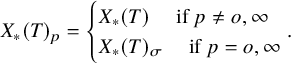 $$\begin{align*}X_*(T)_p=\begin{cases} X_*(T) \quad \text{ if } p\not=o ,\infty \\ X_*(T)_\sigma \quad \text{ if } p=o, \infty \end{cases}\!\!\!\!\!. \end{align*}$$
By [Reference ZhuZh2, Proposition 3.4], for any $\lambda \in X_*(T)$
, there exists a section
$\lambda \in X_*(T)$
, there exists a section $s^\lambda : C\to L_C\mathcal {T}$
, such that for any
$s^\lambda : C\to L_C\mathcal {T}$
, such that for any $p\in C$
, the image of
$p\in C$
, the image of $s^\lambda (p)$
in
$s^\lambda (p)$
in $X_*(T)_p$
is given by
$X_*(T)_p$
is given by
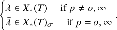 $$\begin{align*}\begin{cases} \lambda\in X_*(T) \quad \text{ if } p\not=o,\infty \\ \bar{\lambda}\in X_*(T)_\sigma \quad \text{ if } p=o,\infty \end{cases}\!\!\!\!\!. \end{align*}$$
This naturally gives rise to C-points in $\operatorname {\mathrm {\mathtt {Gr}}}_{\mathcal {T}, C}$
and
$\operatorname {\mathrm {\mathtt {Gr}}}_{\mathcal {T}, C}$
and $\operatorname {\mathrm {\mathtt {Gr}}}_{\mathcal {G},C}$
, which will still be denoted by
$\operatorname {\mathrm {\mathtt {Gr}}}_{\mathcal {G},C}$
, which will still be denoted by $s^\lambda $
. Following [Reference ZhuZh2, Definition 3.1], for each
$s^\lambda $
. Following [Reference ZhuZh2, Definition 3.1], for each $\lambda \in X_*(T)$
, we define the global Schubert variety
$\lambda \in X_*(T)$
, we define the global Schubert variety $\overline {\operatorname {\mathrm {\mathtt {Gr}}}}_{\mathcal {G},C}^\lambda $
to be the minimal
$\overline {\operatorname {\mathrm {\mathtt {Gr}}}}_{\mathcal {G},C}^\lambda $
to be the minimal $L_C^+\mathcal {G}$
-stable irreducible closed subvariety of
$L_C^+\mathcal {G}$
-stable irreducible closed subvariety of $\operatorname {\mathrm {\mathtt {Gr}}}_{\mathcal {G},C }$
that contains
$\operatorname {\mathrm {\mathtt {Gr}}}_{\mathcal {G},C }$
that contains $s^\lambda $
. Then, [Reference ZhuZh2, Theorem 3] asserts the following.
$s^\lambda $
. Then, [Reference ZhuZh2, Theorem 3] asserts the following.
Theorem 2.4. The global Schubert variety $\overline {\operatorname {\mathrm {\mathtt {Gr}}}}_{\mathcal {G},C}^\lambda $
is flat over C, and for any
$\overline {\operatorname {\mathrm {\mathtt {Gr}}}}_{\mathcal {G},C}^\lambda $
is flat over C, and for any $p\in C$
, the fiber
$p\in C$
, the fiber $\overline {\operatorname {\mathrm {\mathtt {Gr}}}}_{\mathcal {G},p}^\lambda $
is reduced and
$\overline {\operatorname {\mathrm {\mathtt {Gr}}}}_{\mathcal {G},p}^\lambda $
is reduced and
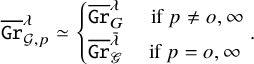 $$\begin{align*}\overline{\operatorname{\mathrm{\mathtt{Gr}}}}_{\mathcal{G},p}^\lambda\simeq \begin{cases} \overline{\operatorname{\mathrm{\mathtt{Gr}}}}^\lambda_G \quad \text{ if } p\not=o,\infty \\ \overline{\operatorname{\mathrm{\mathtt{Gr}}}}_{\mathscr{G}}^{\bar{\lambda} } \quad \text{ if } p=o,\infty \end{cases}\!\!\!\!\!. \end{align*}$$
3 Construction of level one line bundle on
$\mathrm {Bun}_{\mathcal {G}}$

In this section, we keep the assumption that G is of adjoint type with the action of a standard automorphism $\sigma $
.
$\sigma $
.
3.1 Borel-Weil-Bott theorem on
$\operatorname {\mathrm {\mathtt {Gr}}}_{\mathscr {G}}$

Let $\hat {L}(\mathfrak {g},\sigma ):=\mathfrak {g}(\mathcal {K})^\sigma \oplus \mathbb {C} K$
be the twisted affine algebra as a central extension of the twisted loop algebra
$\hat {L}(\mathfrak {g},\sigma ):=\mathfrak {g}(\mathcal {K})^\sigma \oplus \mathbb {C} K$
be the twisted affine algebra as a central extension of the twisted loop algebra $\mathfrak {g}(\mathcal {K})^\sigma $
with the canonical center K, whose Lie bracket is defined as follows:
$\mathfrak {g}(\mathcal {K})^\sigma $
with the canonical center K, whose Lie bracket is defined as follows:
 $$ \begin{align} [x[f]+z K, x'[f'] +z' K] = [x,x' ][ff'] +m^{-1}\mathrm{Res}_{t=0} \, \bigl (({df}) f'\bigr) ( x,x') K, \end{align} $$
for $x[f],x'[f']\in \mathfrak {g}(\mathcal {K})^\sigma $
where
$x[f],x'[f']\in \mathfrak {g}(\mathcal {K})^\sigma $
where $x,x'\in \mathfrak {g}$
,
$x,x'\in \mathfrak {g}$
, $f,f'\in \mathcal {K}$
, and
$f,f'\in \mathcal {K}$
, and $z, z'\in \mathbb {C}$
, and where
$z, z'\in \mathbb {C}$
, and where $\mathrm {Res}_{t=0}$
denotes the coefficient of
$\mathrm {Res}_{t=0}$
denotes the coefficient of $t^{-1}dt$
, and
$t^{-1}dt$
, and $(,)$
is the normalized Killing form on
$(,)$
is the normalized Killing form on $\mathfrak {g}$
(i.e.,
$\mathfrak {g}$
(i.e., $(\check {\theta }, \check {\theta } )=2$
).
$(\check {\theta }, \check {\theta } )=2$
).
We use $P( \sigma ,c)$
to denote the set of highest weights of
$P( \sigma ,c)$
to denote the set of highest weights of $\mathfrak {g}^\sigma $
which parametrizes the integrable highest weight modules of
$\mathfrak {g}^\sigma $
which parametrizes the integrable highest weight modules of $\hat {L}(\mathfrak {g}, \sigma )$
of level c; see [Reference Hong and KumarHK, Section 2]. For each
$\hat {L}(\mathfrak {g}, \sigma )$
of level c; see [Reference Hong and KumarHK, Section 2]. For each $\lambda \in P( \sigma ,c)$
, we denote by
$\lambda \in P( \sigma ,c)$
, we denote by $\mathscr {H}_{ c}(\lambda ) $
the associated integrable highest weight module of
$\mathscr {H}_{ c}(\lambda ) $
the associated integrable highest weight module of $\hat {L}(\mathfrak {g}, \sigma )$
.
$\hat {L}(\mathfrak {g}, \sigma )$
.
Recall that $\{ \lambda _i \,|\, i\in I_\sigma \}$
is the set of fundamental weights of
$\{ \lambda _i \,|\, i\in I_\sigma \}$
is the set of fundamental weights of $\mathfrak {g}^\sigma $
, where we follow the labellings in (2.4). Also,
$\mathfrak {g}^\sigma $
, where we follow the labellings in (2.4). Also, $\{ \, \check {\beta }_i \,|\, i\in I_\sigma \, \}$
is the set of simple coroots of
$\{ \, \check {\beta }_i \,|\, i\in I_\sigma \, \}$
is the set of simple coroots of $\mathfrak {g}^\sigma $
.
$\mathfrak {g}^\sigma $
.
Lemma 3.1. For a standard automorphism $\sigma $
, we have
$\sigma $
, we have
 $$\begin{align*}P(\sigma,1)=\begin{cases}\{ 0\} \quad \quad \text{ if } (\mathfrak{g},m)\not= (A_{2\ell-1}, 2 ), (D_{\ell+1}, 2 ) \\ \{ 0, \lambda_1 \} \quad \quad \text{ if } (\mathfrak{g},m)= (A_{2\ell-1}, 2 ) \\ \{0, \lambda_\ell \} \quad\quad \text{ if } (\mathfrak{g},m)= (D_{\ell+1}, 2 ) \\ \end{cases}\!\!\!\!\!.\end{align*}$$
Proof. We first consider the case when $(\mathfrak {g},m)\not = (A_{2\ell }, 4 )$
. We can read from [Reference Hong and KumarHK, Lemma 2.1], for any
$(\mathfrak {g},m)\not = (A_{2\ell }, 4 )$
. We can read from [Reference Hong and KumarHK, Lemma 2.1], for any $\lambda \in (\mathfrak {h}^\sigma )^\vee $
,
$\lambda \in (\mathfrak {h}^\sigma )^\vee $
, $\lambda \in P(\sigma ,1)$
if and only if
$\lambda \in P(\sigma ,1)$
if and only if
 $$\begin{align*}\langle \lambda, \check{\beta}_i \rangle\in \mathbb{Z}_{\geq 0} \quad \text{ for any } i\in I_\sigma , \end{align*}$$
and $\langle \lambda , \check {\theta }_0 \rangle \leq 1$
, where
$\langle \lambda , \check {\theta }_0 \rangle \leq 1$
, where $\theta _0$
is the highest short root of
$\theta _0$
is the highest short root of $\mathfrak {g}^\sigma $
and
$\mathfrak {g}^\sigma $
and $\check {\theta }_0$
is the coroot of
$\check {\theta }_0$
is the coroot of $\theta _0$
, and hence,
$\theta _0$
, and hence, $\check {\theta }_0$
is the highest coroot of
$\check {\theta }_0$
is the highest coroot of $\mathfrak {g}^\sigma $
. In this case,
$\mathfrak {g}^\sigma $
. In this case, $\lambda \in P( \sigma ,1)$
if and only if
$\lambda \in P( \sigma ,1)$
if and only if $\lambda =0$
or a minuscule dominant weight of
$\lambda =0$
or a minuscule dominant weight of $\mathfrak {g}^\sigma $
(cf. [Reference Besson and HongBH, Lemma 2.13]). Following the labellings in [Reference KacKa, Table Fin, p53], when
$\mathfrak {g}^\sigma $
(cf. [Reference Besson and HongBH, Lemma 2.13]). Following the labellings in [Reference KacKa, Table Fin, p53], when $\mathfrak {g}^\sigma $
is of type
$\mathfrak {g}^\sigma $
is of type $C_\ell $
,
$C_\ell $
, $\lambda _1$
is the only minuscule weight; when
$\lambda _1$
is the only minuscule weight; when $\mathfrak {g}^\sigma $
is of type
$\mathfrak {g}^\sigma $
is of type $B_\ell $
,
$B_\ell $
, $\lambda _\ell $
is the only minuscule weight. Any other nonsimply-laced Lie algebra has no minuscule weight. This finishes the argument of the lemma when
$\lambda _\ell $
is the only minuscule weight. Any other nonsimply-laced Lie algebra has no minuscule weight. This finishes the argument of the lemma when $(\mathfrak {g},m)\not = (A_{2\ell }, 4 )$
.
$(\mathfrak {g},m)\not = (A_{2\ell }, 4 )$
.
Now, we assume that $(\mathfrak {g},m)= (A_{2\ell }, 4 )$
. In this case, it is more convenient to choose a different set of simple roots for
$(\mathfrak {g},m)= (A_{2\ell }, 4 )$
. In this case, it is more convenient to choose a different set of simple roots for $\mathfrak {g}^\sigma $
rather than the one described in (2.4). Namely, we can choose
$\mathfrak {g}^\sigma $
rather than the one described in (2.4). Namely, we can choose
 $$\begin{align*}\{ \alpha_i|_{\mathfrak{h}^\sigma} \,|\, i=1,2,\cdots, \ell-1 \}\cup \{ -\theta|_{\mathfrak{h}^\sigma} \} \end{align*}$$
as a set of simple roots of $\mathfrak {g}^\sigma $
. With this set of simple roots, we can also read from [Reference Hong and KumarHK, Lemma 2.1], for any
$\mathfrak {g}^\sigma $
. With this set of simple roots, we can also read from [Reference Hong and KumarHK, Lemma 2.1], for any $\lambda \in (\mathfrak {h}^\sigma )^\vee $
,
$\lambda \in (\mathfrak {h}^\sigma )^\vee $
, $\lambda \in P(\sigma ,1)$
if and only if
$\lambda \in P(\sigma ,1)$
if and only if $\lambda =0$
.
$\lambda =0$
.
Remark 3.2. It is not true that $0\in P(\sigma ,1)$
for any automorphism
$0\in P(\sigma ,1)$
for any automorphism $\sigma $
. For example,
$\sigma $
. For example, $0\not \in P(\tau ,1)$
, when
$0\not \in P(\tau ,1)$
, when $\mathfrak {g}=A_{2\ell }$
and
$\mathfrak {g}=A_{2\ell }$
and $\tau $
is a diagram automorphism; instead,
$\tau $
is a diagram automorphism; instead, $0\in P(\tau ,2)$
.
$0\in P(\tau ,2)$
.
We define the following map:
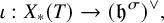 $$ \begin{align} \iota: X_*(T) \to (\mathfrak{h}^\sigma )^\vee , \end{align} $$
such that for any ${\lambda }\in X_*(T) $
,
${\lambda }\in X_*(T) $
, $\iota ({\lambda })(h)=(\lambda , h)$
, where we regard
$\iota ({\lambda })(h)=(\lambda , h)$
, where we regard $\lambda $
as an element in
$\lambda $
as an element in $\mathfrak {h}$
and
$\mathfrak {h}$
and $(,)$
is the normalized Killing form on
$(,)$
is the normalized Killing form on $\mathfrak {h}$
. It is clear that
$\mathfrak {h}$
. It is clear that $\iota (0)=0$
. This map naturally descends to a map
$\iota (0)=0$
. This map naturally descends to a map $X_*(T)_\sigma \to (\mathfrak {h}^\sigma )^\vee $
. By abuse of notation, we still call it
$X_*(T)_\sigma \to (\mathfrak {h}^\sigma )^\vee $
. By abuse of notation, we still call it $\iota $
.
$\iota $
.
Recall some terminology introduced in Section 2.1. $I_\sigma $
is the set parametrizing simple roots of
$I_\sigma $
is the set parametrizing simple roots of $\mathfrak {g}^\sigma $
, and we also defined a map
$\mathfrak {g}^\sigma $
, and we also defined a map $\eta : I\to I_\sigma $
. The set
$\eta : I\to I_\sigma $
. The set $\{ \check {\lambda }_j \,|\, j\in I_\sigma \}$
is the set of fundamental coweights of
$\{ \check {\lambda }_j \,|\, j\in I_\sigma \}$
is the set of fundamental coweights of $\mathfrak {g}^\sigma $
, and
$\mathfrak {g}^\sigma $
, and $\{ \lambda _j \,|\, j\in I_\sigma \}$
is the set of fundamental weights of
$\{ \lambda _j \,|\, j\in I_\sigma \}$
is the set of fundamental weights of $\mathfrak {g}^\sigma $
. We also recall that
$\mathfrak {g}^\sigma $
. We also recall that $\check {\alpha }_i$
is a simple coroot of
$\check {\alpha }_i$
is a simple coroot of $\mathfrak {g}$
for each
$\mathfrak {g}$
for each $i\in I$
, and
$i\in I$
, and $\gamma _j$
is the image of
$\gamma _j$
is the image of $\check {\alpha }_i$
in
$\check {\alpha }_i$
in $X_*(T)_\sigma $
. The following lemma already appears in [Reference HainesHa, Lemma 3.2] in a slighly different setting.
$X_*(T)_\sigma $
. The following lemma already appears in [Reference HainesHa, Lemma 3.2] in a slighly different setting.
Lemma 3.3. For any $j\in I_\sigma $
, we have
$j\in I_\sigma $
, we have
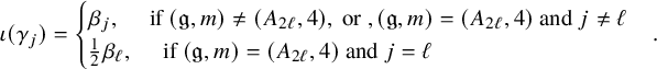 $$\begin{align*}\iota( \gamma_j ) = \begin{cases} \beta_j , \quad \text{ if } (\mathfrak{g}, m)\not= (A_{2\ell}, 4), \text{ or }, (\mathfrak{g}, m)= (A_{2\ell}, 4) \text{ and } j\not= \ell \\ \frac{1}{2} \beta_\ell, \quad \text{ if } (\mathfrak{g}, m)= (A_{2\ell}, 4) \text{ and } j= \ell \end{cases}. \end{align*}$$
Proof. By the definition of $\iota $
, for any
$\iota $
, for any $\gamma _j=\overline {\check {\alpha }}_i$
with
$\gamma _j=\overline {\check {\alpha }}_i$
with $j=\eta (i)$
, and
$j=\eta (i)$
, and $k\in I_\sigma $
, we have the following equalities:
$k\in I_\sigma $
, we have the following equalities:
 $$\begin{align*}\langle \check{\lambda}_k, \gamma_j \rangle= \langle \check{\lambda}_k, \iota( \overline{\check{\alpha}}_i ) \rangle=( \check{\lambda}_k, \check{\alpha}_i )=\langle\check{\lambda}_k, \alpha_i \rangle .\end{align*}$$
Then, this lemma readily follows from the description of fundamental coweights of $\mathfrak {g}^\sigma $
in (2.7) and (2.8).
$\mathfrak {g}^\sigma $
in (2.7) and (2.8).
Recall the set S defined in (2.14).
Lemma 3.4. For any $i\in I$
, we have
$i\in I$
, we have $ \iota (\check {\omega }_i ) =\lambda _{\eta (i)} $
. As a consequence,
$ \iota (\check {\omega }_i ) =\lambda _{\eta (i)} $
. As a consequence, $\iota $
maps
$\iota $
maps $X_*(T)_\sigma ^+$
bijectively into the set of dominant weights of
$X_*(T)_\sigma ^+$
bijectively into the set of dominant weights of $\mathfrak {g}^\sigma $
. Furthermore,
$\mathfrak {g}^\sigma $
. Furthermore, $\iota $
maps S bijectively into
$\iota $
maps S bijectively into $P(\sigma ,1)$
.
$P(\sigma ,1)$
.
Proof. For any $i\in I$
and
$i\in I$
and $j\in I_\sigma $
, we have
$j\in I_\sigma $
, we have
 $$\begin{align*}\langle \iota(\check{\omega }_i), \check{\beta}_j \rangle =\left( \check{\omega}_i, \check{\beta}_j \right)=( \check{\omega}_i, \sum_{a\in \eta^{-1}(i) } \check{\alpha}_a )= \delta_{\eta(i) ,j } .\end{align*}$$
Hence, $\iota (\check {\omega }_i)=\lambda _{\eta (i)}$
.
$\iota (\check {\omega }_i)=\lambda _{\eta (i)}$
.
In view of Lemma 3.1, $\iota $
maps S bijectively into
$\iota $
maps S bijectively into $P(\sigma ,1)$
.
$P(\sigma ,1)$
.
Remark 3.5. In view of Lemma 3.3 and Lemma 3.4, when $(G, m)\not = (A_{2\ell }, 4 )$
, the root systems of
$(G, m)\not = (A_{2\ell }, 4 )$
, the root systems of $\mathfrak {g}^\sigma $
and
$\mathfrak {g}^\sigma $
and $H:=(\check {G})^\tau $
can be naturally identified, where H is discussed in Section 2.3. Namely,
$H:=(\check {G})^\tau $
can be naturally identified, where H is discussed in Section 2.3. Namely, $\{ \, \overline {\check {\omega }}_i \,|\, i\in I \}$
is a set of fundamental weights of H corresponding to
$\{ \, \overline {\check {\omega }}_i \,|\, i\in I \}$
is a set of fundamental weights of H corresponding to $\{ \lambda _j \,|\, j\in I_\sigma \}$
of
$\{ \lambda _j \,|\, j\in I_\sigma \}$
of $\mathfrak {g}^\sigma $
, and the set of simple roots
$\mathfrak {g}^\sigma $
, and the set of simple roots $\{ \, \gamma _j \,|\, j\in I_\sigma \}$
corresponds to
$\{ \, \gamma _j \,|\, j\in I_\sigma \}$
corresponds to $\{\, \beta _j \,|\, j\in I_\sigma \, \}$
of
$\{\, \beta _j \,|\, j\in I_\sigma \, \}$
of $\mathfrak {g}^\sigma $
.
$\mathfrak {g}^\sigma $
.
For any $g\in G(\mathcal {K})^\sigma $
, we can define a Lie algebra automorphism
$g\in G(\mathcal {K})^\sigma $
, we can define a Lie algebra automorphism
 $$ \begin{align} \widehat{ \mathrm{Ad} }_{ g} (x[f]):= \mathrm{Ad}_{g}(x[f]) + \frac{1}{m} \mathrm{Res}_{t=0} ( g^{-1}dg, x[f] ) K , \end{align} $$
for any $x[f]\in \mathfrak {g}(\mathcal {K})^\sigma $
, where
$x[f]\in \mathfrak {g}(\mathcal {K})^\sigma $
, where $(,)$
is the normalized Killing form on
$(,)$
is the normalized Killing form on $\mathfrak {g}$
. By Lemma 3.4,
$\mathfrak {g}$
. By Lemma 3.4, $\iota (\kappa )\in P(\sigma , 1)$
for any
$\iota (\kappa )\in P(\sigma , 1)$
for any $\kappa \in S$
. Thus,
$\kappa \in S$
. Thus, $c\iota (\kappa )\in P(\sigma , c)$
for any level
$c\iota (\kappa )\in P(\sigma , c)$
for any level $c\geq 1$
.
$c\geq 1$
.
Set
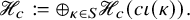 $$ \begin{align} \mathscr{H}_c := \oplus_{\kappa\in S} \mathscr{H}_c(c \iota(\kappa)).\end{align} $$
Let $\tilde {\mathfrak {g}}:= \mathfrak {g}\otimes \mathcal {K}\oplus \mathbb {C} K'\oplus \mathbb {C} d' $
be the untwisted Kac-Moody algebra associated to
$\tilde {\mathfrak {g}}:= \mathfrak {g}\otimes \mathcal {K}\oplus \mathbb {C} K'\oplus \mathbb {C} d' $
be the untwisted Kac-Moody algebra associated to $\mathfrak {g}$
, where
$\mathfrak {g}$
, where $K'$
is the canonical center and
$K'$
is the canonical center and $d'$
is the scaling element. We may define an automorphism
$d'$
is the scaling element. We may define an automorphism $\sigma $
on
$\sigma $
on $\tilde {\mathfrak {g}}$
as follows:
$\tilde {\mathfrak {g}}$
as follows:
 $$\begin{align*}\sigma( x[f(t)] )=\sigma(x)[f(\epsilon t )], \quad \sigma(K')=K', \quad \sigma(d')=d', \end{align*}$$
for any $x[f]\in \mathfrak {g}\otimes \mathcal {K}$
. Then the fixed point Lie algebra
$x[f]\in \mathfrak {g}\otimes \mathcal {K}$
. Then the fixed point Lie algebra $\tilde {\mathfrak {g}}^{\sigma }$
is exactly the twisted Kac-Moody alegbra
$\tilde {\mathfrak {g}}^{\sigma }$
is exactly the twisted Kac-Moody alegbra $\tilde {L}(\mathfrak {g}, \sigma )$
containing
$\tilde {L}(\mathfrak {g}, \sigma )$
containing $\hat {L}(\mathfrak {g}, \sigma )$
as the derived algebra. Following from [Reference KacKa, Theorem 8.7,§8], in this realization, the canonical center K in
$\hat {L}(\mathfrak {g}, \sigma )$
as the derived algebra. Following from [Reference KacKa, Theorem 8.7,§8], in this realization, the canonical center K in $\tilde {L}(\mathfrak {g}, \sigma )$
is equal to
$\tilde {L}(\mathfrak {g}, \sigma )$
is equal to $mK'$
, and the scaling element d in
$mK'$
, and the scaling element d in $\tilde {\mathfrak {g}}$
is equal to
$\tilde {\mathfrak {g}}$
is equal to $d'$
when
$d'$
when $\tilde {\mathfrak {g}}^{\sigma }$
is not
$\tilde {\mathfrak {g}}^{\sigma }$
is not $A_{2\ell }^{(2)}$
, and
$A_{2\ell }^{(2)}$
, and $d=2d'$
when
$d=2d'$
when $\tilde {\mathfrak {g}}^{\sigma }=A_{2\ell }^{(2)}$
.
$\tilde {\mathfrak {g}}^{\sigma }=A_{2\ell }^{(2)}$
.
For any $g\in G(\mathcal {K})$
, one can define an automorphism
$g\in G(\mathcal {K})$
, one can define an automorphism $\widehat {\mathrm {Ad}}_g$
on
$\widehat {\mathrm {Ad}}_g$
on $\tilde {\mathfrak {g}}$
as in [Reference KumarKu, Section 13.2.3]. From the formula
$\tilde {\mathfrak {g}}$
as in [Reference KumarKu, Section 13.2.3]. From the formula $\textit {loc.cit}$
, it is clear that if
$\textit {loc.cit}$
, it is clear that if $g\in G(\mathcal {K})^{\sigma }$
, then
$g\in G(\mathcal {K})^{\sigma }$
, then $\widehat {\mathrm {Ad}}_g$
commutes with
$\widehat {\mathrm {Ad}}_g$
commutes with $\sigma $
. In particular, it follows that
$\sigma $
. In particular, it follows that $\widehat {\mathrm {Ad}}_g$
restricts to an automorphism on
$\widehat {\mathrm {Ad}}_g$
restricts to an automorphism on $\tilde {L}(\mathfrak {g}, \sigma )$
. One may observe easily that, restricting further to
$\tilde {L}(\mathfrak {g}, \sigma )$
. One may observe easily that, restricting further to $\hat {L}(\mathfrak {g}, \sigma )$
, this is exactly the automorphism defined in (3.3).
$\hat {L}(\mathfrak {g}, \sigma )$
, this is exactly the automorphism defined in (3.3).
By demanding that $d\cdot v_\kappa =0$
for each
$d\cdot v_\kappa =0$
for each $\kappa \in S$
, the action
$\kappa \in S$
, the action $\hat {L}(\mathfrak {g},\sigma )$
on
$\hat {L}(\mathfrak {g},\sigma )$
on $\mathscr {H}$
extends uniquely to an action of
$\mathscr {H}$
extends uniquely to an action of $\tilde {L}(\mathfrak {g},\sigma )$
.
$\tilde {L}(\mathfrak {g},\sigma )$
.
Lemma 3.6. For any $g\in G(\mathcal {K})^\sigma $
, there exists an intertwining operator
$g\in G(\mathcal {K})^\sigma $
, there exists an intertwining operator $\rho _g: \mathscr {H}_c\simeq \mathscr {H}_c$
such that
$\rho _g: \mathscr {H}_c\simeq \mathscr {H}_c$
such that
 $$ \begin{align} \rho_g( x[f]\cdot v )= \widehat{ \mathrm{Ad} }_{ g} (x[f]) \cdot \rho_g( v ), \end{align} $$
for any $x[f]\in \mathfrak {g}(\mathcal {K})^\sigma $
and
$x[f]\in \mathfrak {g}(\mathcal {K})^\sigma $
and $v\in \mathscr {H}_c$
. In particular, for any
$v\in \mathscr {H}_c$
. In particular, for any $\kappa \in S$
,
$\kappa \in S$
,
 $$ \begin{align} \widehat{ \mathrm{Ad} }_{n^{-\kappa}}( \mathscr{H}_c(0) )= \mathscr{H}_c(c\iota(\kappa)), \, \text{ and } \, \widehat{ \mathrm{Ad} }_{n^{-\kappa}}( \mathscr{H}_c(c\iota(\kappa)) ) = \mathscr{H}_c(0). \end{align} $$
Proof. Let $G'$
be the simply-connected cover of G, and let
$G'$
be the simply-connected cover of G, and let $p: G'(\mathcal {K})^\sigma \to G(\mathcal {K})^\sigma $
be the induced map. Then,
$p: G'(\mathcal {K})^\sigma \to G(\mathcal {K})^\sigma $
be the induced map. Then,
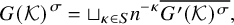 $$ \begin{align} G(\mathcal{K})^\sigma=\sqcup_{\kappa \in S} n^{-\kappa} \overline{G'(\mathcal{K})^\sigma } , \end{align} $$
where $\overline {G'(\mathcal {K})^\sigma }=p(G'(\mathcal {K})^\sigma )$
. By twisted analogue of Faltings Lemma (cf. [Reference Hong and KumarHK, Proposition 10.2]), for any element
$\overline {G'(\mathcal {K})^\sigma }=p(G'(\mathcal {K})^\sigma )$
. By twisted analogue of Faltings Lemma (cf. [Reference Hong and KumarHK, Proposition 10.2]), for any element $g\in \overline {G'(\mathcal {K})^\sigma }$
, there exists an operator
$g\in \overline {G'(\mathcal {K})^\sigma }$
, there exists an operator $\rho _g$
which maps
$\rho _g$
which maps $ \mathscr {H}_c(c\iota (\kappa ))$
to
$ \mathscr {H}_c(c\iota (\kappa ))$
to $\mathscr {H}_c(c\iota (\kappa ))$
with the desired property (3.5), for any
$\mathscr {H}_c(c\iota (\kappa ))$
with the desired property (3.5), for any $\kappa \in S$
. By decomposition (3.7), it suffices to show that, for nonzero
$\kappa \in S$
. By decomposition (3.7), it suffices to show that, for nonzero $\kappa $
,
$\kappa $
, $n^{-\kappa }$
satisfies property (3.6).
$n^{-\kappa }$
satisfies property (3.6).
Assume $\kappa \not =0$
in S. From the table (2.11), the group
$\kappa \not =0$
in S. From the table (2.11), the group $(X_*(T)/{\check {Q}})_\sigma $
is at most of order
$(X_*(T)/{\check {Q}})_\sigma $
is at most of order $2$
. Therefore,
$2$
. Therefore, $n^{-2\kappa }\in \overline {G'(\mathcal {K})^\sigma } $
. For each
$n^{-2\kappa }\in \overline {G'(\mathcal {K})^\sigma } $
. For each $\mathscr {H}_c(c\iota (\kappa ))$
, we denote the action by
$\mathscr {H}_c(c\iota (\kappa ))$
, we denote the action by $\pi _{c, \kappa }: \hat {L}(\mathfrak {g},\sigma )\to \mathrm {End}( \mathscr {H}_c(c\iota (\kappa )) ) $
. Then the property (3.5) for
$\pi _{c, \kappa }: \hat {L}(\mathfrak {g},\sigma )\to \mathrm {End}( \mathscr {H}_c(c\iota (\kappa )) ) $
. Then the property (3.5) for $n^{-2\kappa }$
is equivalent to the existence of an isomorphism of representations,
$n^{-2\kappa }$
is equivalent to the existence of an isomorphism of representations,
 $$ \begin{align} \rho_{n^{-2\kappa}}: (\mathscr{H}_c(c\iota(\kappa) ), \pi_{c,\kappa}) \simeq (\mathscr{H}_c(c\iota(\kappa) ), \pi_{c, \kappa} \circ \widehat{ \mathrm{Ad} }_{n^{-2\kappa}} ) .\end{align} $$
Let $v_\kappa $
be the highest weight vector in
$v_\kappa $
be the highest weight vector in $\mathscr {H}_c(c\iota (\kappa ))$
. Then
$\mathscr {H}_c(c\iota (\kappa ))$
. Then $v_\kappa $
is of
$v_\kappa $
is of $\mathfrak {h}^\sigma $
-weight
$\mathfrak {h}^\sigma $
-weight $c\iota (\kappa )$
. We regard
$c\iota (\kappa )$
. We regard $\check {\beta }_i$
as elements in
$\check {\beta }_i$
as elements in $\mathfrak {h}^\sigma $
. By formula (3.3),
$\mathfrak {h}^\sigma $
. By formula (3.3),
 $$\begin{align*}\widehat{\mathrm{Ad}}_{n^{-\kappa}}( \check{\beta}_i ) = \check{\beta}_i - (\kappa, \check{\beta}_i ) c= \check{\beta}_i - \langle \iota(\kappa), \check{\beta}_i \rangle c. \end{align*}$$
Hence, $v_\kappa $
is of
$v_\kappa $
is of $\mathfrak {h}^\sigma $
-weight 0 and a highest weight vector in the representation
$\mathfrak {h}^\sigma $
-weight 0 and a highest weight vector in the representation
 $$\begin{align*}(\mathscr{H}_c(c\iota(\kappa) ), \pi_{c, \kappa} \circ \widehat{ \mathrm{Ad} }_{n^{-\kappa}} ) .\end{align*}$$
By Schur lemma, there exists an intertwining operator $\rho _{0 \kappa }$
,
$\rho _{0 \kappa }$
,
 $$ \begin{align} \rho_{0 \kappa}: (\mathscr{H}_c(0), \pi_{c, 0} ) \simeq (\mathscr{H}_c(c\iota(\kappa) ), \pi_{c, \kappa} \circ \widehat{ \mathrm{Ad} }_{n^{-\kappa}} ). \end{align} $$
We also can regard $\rho _{0 \kappa }$
as the following intertwining operator
$\rho _{0 \kappa }$
as the following intertwining operator
 $$ \begin{align} \rho_{0 \kappa}: (\mathscr{H}_c(0), \pi_{c, 0} \circ \widehat{ \mathrm{Ad} }_{n^{-\kappa}} ) \simeq (\mathscr{H}_c(c\iota(\kappa) ), \pi_{c, \kappa} \circ \widehat{ \mathrm{Ad} }_{n^{-2\kappa}} ). \end{align} $$
Combining isomorphisms (3.8),(3.10), we get
 $$\begin{align*}(\mathscr{H}_c(c\iota(\kappa)) ,\pi_{c,\kappa}) \xrightarrow{ \rho_{n^{-2\kappa}} } (\mathscr{H}_c(c\iota(\kappa) ) , \pi_{c, \kappa} \circ \widehat{ \mathrm{Ad} }_{n^{-2\kappa}} )\xrightarrow{ (\rho_{0 \kappa} )^{-1} } (\mathscr{H}_{c}(0) , \pi_{c, 0} \circ \widehat{ \mathrm{Ad} }_{n^{-\kappa}} ). \end{align*}$$
We define $ \rho _{n^{-\kappa }}$
to be the following operator:
$ \rho _{n^{-\kappa }}$
to be the following operator:
 $$\begin{align*}\rho_{n^{-\kappa}}=(\rho_{0 \kappa}, (\rho_{0 \kappa} )^{-1} \circ \rho_{n^{-2\kappa}} ): \mathscr{H}_c(0) \oplus \mathscr{H}_c(c\iota(\kappa) )\simeq \mathscr{H}_c(0 ) \oplus \mathscr{H}_c(c\iota(\kappa)). \end{align*}$$
The map $\rho _{n^{-\kappa }}$
satisfies property (3.5).
$\rho _{n^{-\kappa }}$
satisfies property (3.5).
As discussed in Section 2.2, the components of $\operatorname {\mathrm {\mathtt {Gr}}}_{{\mathscr {G}} }$
are parametrized by elements in
$\operatorname {\mathrm {\mathtt {Gr}}}_{{\mathscr {G}} }$
are parametrized by elements in $(X_*(T)/{\check {Q}})_\sigma $
. Moreover,
$(X_*(T)/{\check {Q}})_\sigma $
. Moreover, $\operatorname {\mathrm {\mathtt {Gr}}}_{\mathscr {G}} = \sqcup _{\kappa \in S} \operatorname {\mathrm {\mathtt {Gr}}}_{{\mathscr {G}} , \kappa } $
, where S is defined in (2.14).
$\operatorname {\mathrm {\mathtt {Gr}}}_{\mathscr {G}} = \sqcup _{\kappa \in S} \operatorname {\mathrm {\mathtt {Gr}}}_{{\mathscr {G}} , \kappa } $
, where S is defined in (2.14).
Let ${\mathscr {G}}'$
be the parahoric group scheme
${\mathscr {G}}'$
be the parahoric group scheme $\mathrm {Res}_{\mathcal {O}/\bar {\mathcal {O} }}(G^{\prime }_{\mathcal {O}})^\sigma $
(
$\mathrm {Res}_{\mathcal {O}/\bar {\mathcal {O} }}(G^{\prime }_{\mathcal {O}})^\sigma $
( $G'$
is the simply-connected cover of G), and let
$G'$
is the simply-connected cover of G), and let $L^+{\mathscr {G}}'$
(resp.
$L^+{\mathscr {G}}'$
(resp. $L{\mathscr {G}}' $
) denote the jet group scheme (resp. loop group scheme) of
$L{\mathscr {G}}' $
) denote the jet group scheme (resp. loop group scheme) of ${\mathscr {G}}'$
. The group
${\mathscr {G}}'$
. The group $L{\mathscr {G}}$
acts on
$L{\mathscr {G}}$
acts on $L{\mathscr {G}}'$
by conjugation. Set
$L{\mathscr {G}}'$
by conjugation. Set
 $$\begin{align*}L^+{\mathscr{G}}^{\prime}_\kappa:=\mathrm{Ad}_{n^{-\kappa}}( L^+{\mathscr{G}} ').\end{align*}$$
Then, $L^+{\mathscr {G}} ^{\prime }_\kappa $
is a subgroup scheme of
$L^+{\mathscr {G}} ^{\prime }_\kappa $
is a subgroup scheme of $L{\mathscr {G}} '$
. We have
$L{\mathscr {G}} '$
. We have
 $$ \begin{align} \operatorname{\mathrm{\mathtt{Gr}}}_{{\mathscr{G}} , \kappa}\simeq L{\mathscr{G}} '/L^+{\mathscr{G}} _\kappa'. \end{align} $$
By the twisted analogue of Faltings lemma (cf. [Reference Hong and KumarHK, Proposition 10.2]), there exists a group homomorphism $ L {{\mathscr {G}}'} \to \mathrm {PGL} ( \mathscr {H}_1(0) ) $
. Consider the central extension
$ L {{\mathscr {G}}'} \to \mathrm {PGL} ( \mathscr {H}_1(0) ) $
. Consider the central extension
 $$ \begin{align} 1\to \mathbb{G}_m \to \mathrm{GL}( \mathscr{H}_1(0) ) \to \mathrm{PGL} ( \mathscr{H}_1(0) ) \to 1. \end{align} $$
The pull-back of (3.12) to $L{ {\mathscr {G}}}'$
defines the following canonical central extension of
$L{ {\mathscr {G}}}'$
defines the following canonical central extension of $L{\mathscr {G}}'$
:
$L{\mathscr {G}}'$
:
 $$ \begin{align} 1\to \mathbb{G}_m \to \widehat{L { {\mathscr{G}}' } } \to L{{\mathscr{G}}'} \to 1. \end{align} $$
It is known that $\widehat {L{{\mathscr {G}}'} }$
is a Kac-Moody group of twisted type (up to a scaling multiplicative group) in the sense of Kumar and Mathieu; see [Reference Pappas and RapoportPR, §9f]. Let
$\widehat {L{{\mathscr {G}}'} }$
is a Kac-Moody group of twisted type (up to a scaling multiplicative group) in the sense of Kumar and Mathieu; see [Reference Pappas and RapoportPR, §9f]. Let $\widehat {L^+{\mathscr {G}} ^{\prime }_\kappa }$
denote the preimage of
$\widehat {L^+{\mathscr {G}} ^{\prime }_\kappa }$
denote the preimage of $L^+{\mathscr {G}} ^{\prime }_\kappa $
in
$L^+{\mathscr {G}} ^{\prime }_\kappa $
in $\widehat {L{{\mathscr {G}}'} }$
via the projection map
$\widehat {L{{\mathscr {G}}'} }$
via the projection map $\widehat {L{{\mathscr {G}}'} } \to L{{\mathscr {G}}'} $
. As the same proof as in [Reference Besson and HongBH, Lemma 2.19],
$\widehat {L{{\mathscr {G}}'} } \to L{{\mathscr {G}}'} $
. As the same proof as in [Reference Besson and HongBH, Lemma 2.19], $\widehat {L^+{\mathscr {G}} ^{\prime }_\kappa } $
is a parabolic subgroup in
$\widehat {L^+{\mathscr {G}} ^{\prime }_\kappa } $
is a parabolic subgroup in $\widehat {L{{\mathscr {G}}'} }$
; moreover,
$\widehat {L{{\mathscr {G}}'} }$
; moreover,
 $$ \begin{align} \operatorname{\mathrm{\mathtt{Gr}}}_{{\mathscr{G}} , \kappa} \simeq \widehat{L{{\mathscr{G}}'} }/ \widehat{L^+{\mathscr{G}} ^{\prime}_\kappa } \end{align} $$
(i.e., $\operatorname {\mathrm {\mathtt {Gr}}}_{{\mathscr {G}} , \kappa } $
is a partial flag variety of the Kac-Moody group
$\operatorname {\mathrm {\mathtt {Gr}}}_{{\mathscr {G}} , \kappa } $
is a partial flag variety of the Kac-Moody group $\widehat {L{{\mathscr {G}}'} }$
).
$\widehat {L{{\mathscr {G}}'} }$
).
Proposition 3.7. There exists a line bundle $\mathscr {L}$
on
$\mathscr {L}$
on $\operatorname {\mathrm {\mathtt {Gr}}}_{\mathscr {G}}$
such that
$\operatorname {\mathrm {\mathtt {Gr}}}_{\mathscr {G}}$
such that $\mathscr {L}$
is of level one on each component of
$\mathscr {L}$
is of level one on each component of $\operatorname {\mathrm {\mathtt {Gr}}}_{\mathscr {G}}$
.
$\operatorname {\mathrm {\mathtt {Gr}}}_{\mathscr {G}}$
.
Proof. We first consider the simply-connected cover $G'$
of G. By [Reference Hong and KumarHK, Theorem 10.7 (1)], there exists a canonical splitting of
$G'$
of G. By [Reference Hong and KumarHK, Theorem 10.7 (1)], there exists a canonical splitting of $\widehat {L{{\mathscr {G}}'} } \to L{{\mathscr {G}} '}$
in the central extension (3.12) over
$\widehat {L{{\mathscr {G}}'} } \to L{{\mathscr {G}} '}$
in the central extension (3.12) over $L^+ {{\mathscr {G}}'}$
. We may define a line bundle
$L^+ {{\mathscr {G}}'}$
. We may define a line bundle $\mathscr {L}$
on
$\mathscr {L}$
on $\operatorname {\mathrm {\mathtt {Gr}}}_{{\mathscr {G}}'}= \widehat {L{\mathscr {G}}'}/ \widehat {L^+ {\mathscr {G}}'}$
via the character
$\operatorname {\mathrm {\mathtt {Gr}}}_{{\mathscr {G}}'}= \widehat {L{\mathscr {G}}'}/ \widehat {L^+ {\mathscr {G}}'}$
via the character $ \widehat {L^+ {\mathscr {G}}'}:= \mathbb {G}_m\times L^+ {\mathscr {G}}'\to \mathbb {G}_m$
defined via the first projection. In fact, as the argument in [Reference Laszlo and SorgerLS, Lemma 4.1], this line bundle is the ample generator of
$ \widehat {L^+ {\mathscr {G}}'}:= \mathbb {G}_m\times L^+ {\mathscr {G}}'\to \mathbb {G}_m$
defined via the first projection. In fact, as the argument in [Reference Laszlo and SorgerLS, Lemma 4.1], this line bundle is the ample generator of $\mathrm { Pic}(\operatorname {\mathrm {\mathtt {Gr}}}_{{\mathscr {G}}'})$
of level 1. This finishes the proof of part (1).
$\mathrm { Pic}(\operatorname {\mathrm {\mathtt {Gr}}}_{{\mathscr {G}}'})$
of level 1. This finishes the proof of part (1).
We now consider the case when G is of adjoint type. Since the neutral component $\operatorname {\mathrm {\mathtt {Gr}}}_{\mathscr {G }, \circ }$
is isomorphic to
$\operatorname {\mathrm {\mathtt {Gr}}}_{\mathscr {G }, \circ }$
is isomorphic to $\operatorname {\mathrm {\mathtt {Gr}}}_{{\mathscr {G}}' }$
, we get the level one line bundle on
$\operatorname {\mathrm {\mathtt {Gr}}}_{{\mathscr {G}}' }$
, we get the level one line bundle on $\operatorname {\mathrm {\mathtt {Gr}}}_{{\mathscr {G}}, \circ }$
induced from the one on
$\operatorname {\mathrm {\mathtt {Gr}}}_{{\mathscr {G}}, \circ }$
induced from the one on $\operatorname {\mathrm {\mathtt {Gr}}}_{{\mathscr {G}}' }$
. For any other component
$\operatorname {\mathrm {\mathtt {Gr}}}_{{\mathscr {G}}' }$
. For any other component $\operatorname {\mathrm {\mathtt {Gr}}}_{{\mathscr {G}},\kappa }$
, by (3.14), we have an isomorphism
$\operatorname {\mathrm {\mathtt {Gr}}}_{{\mathscr {G}},\kappa }$
, by (3.14), we have an isomorphism $\operatorname {\mathrm {\mathtt {Gr}}}_{{\mathscr {G}}, \circ }\simeq \operatorname {\mathrm {\mathtt {Gr}}}_{{\mathscr {G}}, \kappa }$
. Therefore, this gives rise to the level one line bundle on
$\operatorname {\mathrm {\mathtt {Gr}}}_{{\mathscr {G}}, \circ }\simeq \operatorname {\mathrm {\mathtt {Gr}}}_{{\mathscr {G}}, \kappa }$
. Therefore, this gives rise to the level one line bundle on $\operatorname {\mathrm {\mathtt {Gr}}}_{{\mathscr {G}}, \kappa }$
.
$\operatorname {\mathrm {\mathtt {Gr}}}_{{\mathscr {G}}, \kappa }$
.
The line bundle $\mathscr {L}$
on
$\mathscr {L}$
on $\operatorname {\mathrm {\mathtt {Gr}}}_{{\mathscr {G}} }$
naturally has a
$\operatorname {\mathrm {\mathtt {Gr}}}_{{\mathscr {G}} }$
naturally has a $\widehat {L{{\mathscr {G}}'} }$
-equivariant structure, since
$\widehat {L{{\mathscr {G}}'} }$
-equivariant structure, since $\mathscr {L}$
admits a unique
$\mathscr {L}$
admits a unique $\widehat {L{{\mathscr {G}}'} }$
-equivariant structure on each component of
$\widehat {L{{\mathscr {G}}'} }$
-equivariant structure on each component of $\operatorname {\mathrm {\mathtt {Gr}}}_{\mathscr {G}}$
as a partial flag variety of
$\operatorname {\mathrm {\mathtt {Gr}}}_{\mathscr {G}}$
as a partial flag variety of $\widehat {L{{\mathscr {G}}'} }$
.
$\widehat {L{{\mathscr {G}}'} }$
.
Theorem 3.8. As representations of $\hat {L}(\mathfrak {g},\sigma )$
, we have
$\hat {L}(\mathfrak {g},\sigma )$
, we have $ H^0(\operatorname {\mathrm {\mathtt {Gr}}}_{{\mathscr {G}} }, \mathscr {L}^c )^\vee \simeq \mathscr {H}_c$
, where
$ H^0(\operatorname {\mathrm {\mathtt {Gr}}}_{{\mathscr {G}} }, \mathscr {L}^c )^\vee \simeq \mathscr {H}_c$
, where $\mathscr {L}^c$
is the c-th power of
$\mathscr {L}^c$
is the c-th power of $\mathscr {L}$
.
$\mathscr {L}$
.
Proof. By [Reference Pappas and RapoportPR, §9f], $\operatorname {\mathrm {\mathtt {Gr}}}_{{\mathscr {G}} }$
can be identified with the partial flag variety of the Kac-Moody group
$\operatorname {\mathrm {\mathtt {Gr}}}_{{\mathscr {G}} }$
can be identified with the partial flag variety of the Kac-Moody group $\widehat {L{{\mathscr {G}}'} }$
constructed by Kumar [Reference KumarKu]. Then, affine Borel-Weil-Bott theorem for Kac-Moody group (cf. [Reference KumarKu, Theorem 8.3.11]), the theorem follows.
$\widehat {L{{\mathscr {G}}'} }$
constructed by Kumar [Reference KumarKu]. Then, affine Borel-Weil-Bott theorem for Kac-Moody group (cf. [Reference KumarKu, Theorem 8.3.11]), the theorem follows.
Let $v_0$
be the highest weight vector in
$v_0$
be the highest weight vector in $\mathscr {H}_c $
. For any
$\mathscr {H}_c $
. For any $\bar {\lambda }\in X_*(T)_\sigma $
, we define
$\bar {\lambda }\in X_*(T)_\sigma $
, we define
 $$ \begin{align} v_{\bar{\lambda}}:= \rho_{n^{\lambda} }(v_0) , \end{align} $$
where $ \rho _{n^{\lambda } }$
in defined in Lemma 3.6. Then
$ \rho _{n^{\lambda } }$
in defined in Lemma 3.6. Then $ v_{\bar {\lambda }}$
is independent of the choice of the representative
$ v_{\bar {\lambda }}$
is independent of the choice of the representative $\lambda $
in
$\lambda $
in $X_*(T)$
and is well defined up to a nonzero scalar.
$X_*(T)$
and is well defined up to a nonzero scalar.
Lemma 3.9. The $\mathfrak {h}^\sigma $
-weight of the vector
$\mathfrak {h}^\sigma $
-weight of the vector $v_{\bar {\lambda }}$
is
$v_{\bar {\lambda }}$
is $-c\iota (\bar {\lambda })$
.
$-c\iota (\bar {\lambda })$
.
Proof. For any $h\in \mathfrak {h}^\sigma $
, by Lemma 3.6,
$h\in \mathfrak {h}^\sigma $
, by Lemma 3.6,
 $$\begin{align*}h\cdot v_{\bar{\lambda}}= h\cdot \rho_{n^\lambda} (v_0)= \rho_{n^\lambda} ( \widehat{ \mathrm{Ad} }_{ n^{-\lambda}} ( h ) v_0 ). \end{align*}$$
By the formula (3.3), we have
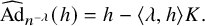 $$\begin{align*}\widehat{ \mathrm{Ad} }_{ n^{-\lambda}} ( h ) = h-\langle \lambda, h \rangle K. \end{align*}$$
It follows that
 $$\begin{align*}h\cdot v_{\bar{\lambda}}= - \langle \lambda, h\rangle c v_{\bar{\lambda}}= -c\iota(\lambda)(h)v_{\bar{\lambda}} .\end{align*}$$
This concludes the proof of the lemma.
Definition 3.10. For any dominant $\bar {\lambda }\in X_*(T)^+_\sigma $
, we define the twisted affine Demazure module
$\bar {\lambda }\in X_*(T)^+_\sigma $
, we define the twisted affine Demazure module $D(c, \bar {\lambda })$
as the following
$D(c, \bar {\lambda })$
as the following $\mathfrak {g}[t]^\sigma $
-module,
$\mathfrak {g}[t]^\sigma $
-module,
 $$\begin{align*}D(c, \bar{\lambda}):=U(\mathfrak{g}[t]^\sigma)v_{\bar{\lambda}}. \end{align*}$$
In view of Lemma 3.9, $D(c, \bar {\lambda })$
contains an irreducible representation
$D(c, \bar {\lambda })$
contains an irreducible representation $V({-c\iota (\lambda )})$
of
$V({-c\iota (\lambda )})$
of $\mathfrak {g}^\sigma $
of lowest weight
$\mathfrak {g}^\sigma $
of lowest weight $-c\iota (\lambda )$
. The following theorem follows from [Reference KumarKu, Theorem 8.2.2 (a)].
$-c\iota (\lambda )$
. The following theorem follows from [Reference KumarKu, Theorem 8.2.2 (a)].
Theorem 3.11. As $\mathfrak {g}[t]^\sigma $
-modules,
$\mathfrak {g}[t]^\sigma $
-modules, $H^0(\overline {\operatorname {\mathrm {\mathtt {Gr}}}}^{\bar {\lambda }}_{\mathscr {G}} , \mathscr {L}^c )^\vee \simeq D(c, \bar {\lambda })$
.
$H^0(\overline {\operatorname {\mathrm {\mathtt {Gr}}}}^{\bar {\lambda }}_{\mathscr {G}} , \mathscr {L}^c )^\vee \simeq D(c, \bar {\lambda })$
.
3.2 Construction of level one line bundles on
$\mathrm {Bun}_{\mathcal {G}}$

In this subsection, we consider the parahoric Bruhat-Tits group scheme $\mathcal {G}:= \mathrm {Res}_{C / \bar {C} }(G\times C )^\Gamma $
over
$\mathcal {G}:= \mathrm {Res}_{C / \bar {C} }(G\times C )^\Gamma $
over $\bar {C}$
as in the setting of Section 2.4.
$\bar {C}$
as in the setting of Section 2.4.
Let $\mathrm {Bun}_{\mathcal {G}}$
be the moduli stack of
$\mathrm {Bun}_{\mathcal {G}}$
be the moduli stack of $\mathcal {G}$
-torsors on
$\mathcal {G}$
-torsors on $\bar {C}$
. It is known that
$\bar {C}$
. It is known that $\mathrm {Bun}_{\mathcal {G}}$
is a smooth Artin stack (cf. [Reference HeinlothHe, Theorem 1]). By [Reference HeinlothHe, Theorem 3], the Picard group
$\mathrm {Bun}_{\mathcal {G}}$
is a smooth Artin stack (cf. [Reference HeinlothHe, Theorem 1]). By [Reference HeinlothHe, Theorem 3], the Picard group $ \mathrm {Pic}(\mathrm {Bun}_{\mathcal {G}} ) $
of
$ \mathrm {Pic}(\mathrm {Bun}_{\mathcal {G}} ) $
of $\mathrm {Bun}_{\mathcal {G}}$
is isomorphic to
$\mathrm {Bun}_{\mathcal {G}}$
is isomorphic to $\mathbb {Z}$
, since the group
$\mathbb {Z}$
, since the group $X^*(\mathcal {G}|_{y})$
of characters for
$X^*(\mathcal {G}|_{y})$
of characters for $\mathcal {G}|_{y}$
is trivial for any
$\mathcal {G}|_{y}$
is trivial for any $y\in \bar {C}$
. In this subsection, we will construct the ample generator
$y\in \bar {C}$
. In this subsection, we will construct the ample generator $\mathcal {L}\in \mathrm {Pic}(\mathrm {Bun}_{\mathcal {G}} ) $
when G is simply-connected, and we will construct a level one line bundle on every component of
$\mathcal {L}\in \mathrm {Pic}(\mathrm {Bun}_{\mathcal {G}} ) $
when G is simply-connected, and we will construct a level one line bundle on every component of $\operatorname {\mathrm {\mathtt {Gr}}}_{\mathcal {G}, C }$
when G is of adjoint type.
$\operatorname {\mathrm {\mathtt {Gr}}}_{\mathcal {G}, C }$
when G is of adjoint type.
By Lemma 3.1, we have $0\in P(\sigma ,1)$
for any standard automorphism
$0\in P(\sigma ,1)$
for any standard automorphism $\sigma $
. Recall that
$\sigma $
. Recall that $\mathscr {H}_1(0)$
is the basic representation of level one associated to
$\mathscr {H}_1(0)$
is the basic representation of level one associated to $0\in P(\sigma ,1)$
.
$0\in P(\sigma ,1)$
.
We now define the following space of twisted covacua of level one,
 $$ \begin{align} \mathscr{V}_{C, \sigma }( 0):= \frac{ \mathscr{H}_{1}(0) } { \mathfrak{g}[ t^{-1} ]^\sigma \cdot \mathscr{H}_{1} (0) } , \end{align} $$
where $\mathfrak {g}[ t^{-1} ]^\sigma $
is the Lie subalgebra of
$\mathfrak {g}[ t^{-1} ]^\sigma $
is the Lie subalgebra of $\hat {L}(\mathfrak {g},\sigma )$
.
$\hat {L}(\mathfrak {g},\sigma )$
.
Lemma 3.12. The dimension of the vector space $ \mathscr {V}_{C, \sigma }( 0)$
is 1.
$ \mathscr {V}_{C, \sigma }( 0)$
is 1.
Proof. Let $v_0$
be the highest weight vector in
$v_0$
be the highest weight vector in $\mathscr {H}_{1} (0)$
. Then
$\mathscr {H}_{1} (0)$
. Then
 $$\begin{align*}\mathscr{H}_{1}(0)=U( (t^{-1}\mathfrak{g}[t^{-1}] )^\sigma ) \cdot v_0 =U( (t^{-1}\mathfrak{g}[t^{-1}] )^\sigma ) (t^{-1}\mathfrak{g}[t^{-1}] )^\sigma v_0\oplus \mathbb{C} v_0 ,\end{align*}$$
where $U( (t^{-1}\mathfrak {g}[t^{-1}] )^\sigma ) $
denotes the universal enveloping algebra of
$U( (t^{-1}\mathfrak {g}[t^{-1}] )^\sigma ) $
denotes the universal enveloping algebra of $(t^{-1}\mathfrak {g}[t^{-1}] )^\sigma $
. We can write
$(t^{-1}\mathfrak {g}[t^{-1}] )^\sigma $
. We can write $\mathfrak {g}[t^{-1}]^\sigma =\mathfrak {g}^\sigma \oplus (t^{-1}\mathfrak {g}[t^{-1}] )^\sigma $
. Hence,
$\mathfrak {g}[t^{-1}]^\sigma =\mathfrak {g}^\sigma \oplus (t^{-1}\mathfrak {g}[t^{-1}] )^\sigma $
. Hence,
 $$ \begin{align*} \mathfrak{g}[t^{-1}]^\sigma\cdot \mathscr{H}_{1}(0) &= \mathfrak{g}^\sigma\cdot U( (t^{-1}\mathfrak{g}[t^{-1}] )^\sigma ) (t^{-1}\mathfrak{g}[t^{-1}] )^\sigma v_0 + U( (t^{-1}\mathfrak{g}[t^{-1}] )^\sigma ) (t^{-1}\mathfrak{g}[t^{-1}] )^\sigma v_0 \\ &= U( (t^{-1}\mathfrak{g}[t^{-1}] )^\sigma ) (t^{-1}\mathfrak{g}[t^{-1}] )^\sigma v_0 , \end{align*} $$
where the first equality holds since $\mathfrak {g}^\sigma \cdot v_0=0$
, and the second equality holds since
$\mathfrak {g}^\sigma \cdot v_0=0$
, and the second equality holds since $\mathfrak {g}^\sigma $
normalizes
$\mathfrak {g}^\sigma $
normalizes $(t^{-1}\mathfrak {g}[t^{-1}] )^\sigma $
under the Lie bracket. Therefore,
$(t^{-1}\mathfrak {g}[t^{-1}] )^\sigma $
under the Lie bracket. Therefore, $\dim \mathscr {V}_{C, \sigma }( 0)=1$
.
$\dim \mathscr {V}_{C, \sigma }( 0)=1$
.
Let $G' $
be the simply-connected cover of G. Recall the Heinloth uniformization theorem for
$G' $
be the simply-connected cover of G. Recall the Heinloth uniformization theorem for ${ \mathcal {G}'} := \mathrm {Res}_{C/ \bar {C} }(G' \times C)^\Gamma $
over the affine line
${ \mathcal {G}'} := \mathrm {Res}_{C/ \bar {C} }(G' \times C)^\Gamma $
over the affine line $\bar {C}\backslash \bar {o}$
(cf. [Reference HeinlothHe]),
$\bar {C}\backslash \bar {o}$
(cf. [Reference HeinlothHe]),
 $$\begin{align*}\mathrm{Bun}_{{ \mathcal{G}'} } \simeq G' [t^{-1}]^\sigma \backslash \operatorname{\mathrm{\mathtt{Gr}}}_{{ {\mathscr{G}} '} } ,\end{align*}$$
where $ \operatorname {\mathrm {\mathtt {Gr}}}_{{ {\mathscr {G}} '} }$
denotes the affine Grassmannian of
$ \operatorname {\mathrm {\mathtt {Gr}}}_{{ {\mathscr {G}} '} }$
denotes the affine Grassmannian of ${\mathscr {G}} ':= \mathrm {Res}_{ \mathcal {O}/ \bar { \mathcal {O} } } (G^{\prime }_{\mathcal {O}})^\sigma $
, and
${\mathscr {G}} ':= \mathrm {Res}_{ \mathcal {O}/ \bar { \mathcal {O} } } (G^{\prime }_{\mathcal {O}})^\sigma $
, and $ G'[t^{-1}]^\sigma \backslash \operatorname {\mathrm {\mathtt {Gr}}}_{ { {\mathscr {G}}'} }$
denotes the fppf quotient.
$ G'[t^{-1}]^\sigma \backslash \operatorname {\mathrm {\mathtt {Gr}}}_{ { {\mathscr {G}}'} }$
denotes the fppf quotient.
Theorem 3.13. The line bundle $\mathscr {L}$
descends to a line bundle
$\mathscr {L}$
descends to a line bundle $\mathcal {L}$
on
$\mathcal {L}$
on $ \mathrm {Bun}_{{ \mathcal {G}' } }$
.
$ \mathrm {Bun}_{{ \mathcal {G}' } }$
.
Proof. Let $\mathscr {L}$
be the level one line bundle on
$\mathscr {L}$
be the level one line bundle on $\operatorname {\mathrm {\mathtt {Gr}}}_{{\mathscr {G}}' }$
constructed from Proposition 3.7. To show that the line bundle
$\operatorname {\mathrm {\mathtt {Gr}}}_{{\mathscr {G}}' }$
constructed from Proposition 3.7. To show that the line bundle $\mathscr {L}$
can descend to
$\mathscr {L}$
can descend to $\mathrm {Bun}_{\mathcal {G}' }$
, as in the argument in [Reference SorgerSo], it suffices to show that there is a
$\mathrm {Bun}_{\mathcal {G}' }$
, as in the argument in [Reference SorgerSo], it suffices to show that there is a $G'[t^{-1}]^\sigma $
-linearization on
$G'[t^{-1}]^\sigma $
-linearization on $\mathscr {L}$
. This is equivalent to the splitting of the central extension (3.13) over
$\mathscr {L}$
. This is equivalent to the splitting of the central extension (3.13) over $G'[t^{-1}]^\sigma $
. We use the same argument as in [Reference SorgerSo, Proposition 3.3], since the vector space
$G'[t^{-1}]^\sigma $
. We use the same argument as in [Reference SorgerSo, Proposition 3.3], since the vector space $\mathscr {V}_{C, \sigma }( 0)$
is nonvanishing by Lemma 3.12, the central extension (3.13) splits over
$\mathscr {V}_{C, \sigma }( 0)$
is nonvanishing by Lemma 3.12, the central extension (3.13) splits over $G'[t^{-1}]^\sigma $
.
$G'[t^{-1}]^\sigma $
.
We consider the projection map $\mathrm {pr}: \operatorname {\mathrm {\mathtt {Gr}}}_{\mathcal {G}', C }\to \mathrm {Bun}_{\mathcal {G}'} $
. By abuse of notation, we still denote by
$\mathrm {pr}: \operatorname {\mathrm {\mathtt {Gr}}}_{\mathcal {G}', C }\to \mathrm {Bun}_{\mathcal {G}'} $
. By abuse of notation, we still denote by $\mathcal {L}$
the line bundle on
$\mathcal {L}$
the line bundle on $ \operatorname {\mathrm {\mathtt {Gr}}}_{\mathcal {G}', C }$
pulling-back from
$ \operatorname {\mathrm {\mathtt {Gr}}}_{\mathcal {G}', C }$
pulling-back from $\mathcal {L}$
on
$\mathcal {L}$
on $\mathrm {Bun}_{\mathcal {G}'} $
.
$\mathrm {Bun}_{\mathcal {G}'} $
.
Corollary 3.14. The restriction of the line bundle $\mathcal {L}$
to the fiber
$\mathcal {L}$
to the fiber $\operatorname {\mathrm {\mathtt {Gr}}}_{\mathcal {G}', p }$
is the ample generator of
$\operatorname {\mathrm {\mathtt {Gr}}}_{\mathcal {G}', p }$
is the ample generator of $\mathrm {Pic} (\operatorname {\mathrm {\mathtt {Gr}}}_{\mathcal {G}', p })$
, for any
$\mathrm {Pic} (\operatorname {\mathrm {\mathtt {Gr}}}_{\mathcal {G}', p })$
, for any $p\in C$
.
$p\in C$
.
Proof. It follows from Theorem 3.13 and [Reference ZhuZh2, Proposition 4.1].
The following theorem is interesting by itself but will not be used in this paper.
Theorem 3.15. There is a natural isomorphism
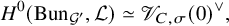 $$\begin{align*}H^0(\mathrm{Bun}_{\mathcal{G}'}, \mathcal{L} )\simeq \mathscr{V}_{C, \sigma }( 0)^\vee, \end{align*}$$
where $\mathscr {V}_{C, \sigma }( 0)^\vee $
denotes the dual of
$\mathscr {V}_{C, \sigma }( 0)^\vee $
denotes the dual of $\mathscr {V}_{C, \sigma }( 0)$
. In particular,
$\mathscr {V}_{C, \sigma }( 0)$
. In particular,
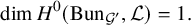 $$\begin{align*}\dim H^0(\mathrm{Bun}_{\mathcal{G}'}, \mathcal{L} )=1.\end{align*}$$
Proof. The theorem follows from the same argument as in [Reference Hong and KumarHK, Theorem 12.1].
Now, we would like to construct the line bundle $\cal {L}$
of level one on
$\cal {L}$
of level one on $\operatorname {\mathrm {\mathtt {Gr}}}_{\mathcal {G} , C}$
, where
$\operatorname {\mathrm {\mathtt {Gr}}}_{\mathcal {G} , C}$
, where $\mathcal {G} =\mathrm {Res}_{C/\bar {C} }(G_C)^\sigma $
with G of adjoint type.
$\mathcal {G} =\mathrm {Res}_{C/\bar {C} }(G_C)^\sigma $
with G of adjoint type.
Theorem 3.16. There exists a line bundle $\mathcal {L}$
on
$\mathcal {L}$
on $\operatorname {\mathrm {\mathtt {Gr}}}_{ \mathcal {G} , C } $
such that the restriction of
$\operatorname {\mathrm {\mathtt {Gr}}}_{ \mathcal {G} , C } $
such that the restriction of $\mathcal {L}$
to the fiber
$\mathcal {L}$
to the fiber $\operatorname {\mathrm {\mathtt {Gr}}}_{\mathcal {G}, p }$
is the level one line bundle on
$\operatorname {\mathrm {\mathtt {Gr}}}_{\mathcal {G}, p }$
is the level one line bundle on $\operatorname {\mathrm {\mathtt {Gr}}}_{\mathcal {G}, p }$
, for any
$\operatorname {\mathrm {\mathtt {Gr}}}_{\mathcal {G}, p }$
, for any $p\in C$
.
$p\in C$
.
Proof. Set $\mathring {C}=C\backslash \{o, \infty \}$
. Then,
$\mathring {C}=C\backslash \{o, \infty \}$
. Then, $\operatorname {\mathrm {\mathtt {Gr}}}_{\mathcal {G}, \mathring {C}}:=\operatorname {\mathrm {\mathtt {Gr}}}_{\mathcal {G}, C}|_{\mathring {C}} \simeq \operatorname {\mathrm {\mathtt {Gr}}}_G\times \mathring {C}$
. Let M be the set consisting of
$\operatorname {\mathrm {\mathtt {Gr}}}_{\mathcal {G}, \mathring {C}}:=\operatorname {\mathrm {\mathtt {Gr}}}_{\mathcal {G}, C}|_{\mathring {C}} \simeq \operatorname {\mathrm {\mathtt {Gr}}}_G\times \mathring {C}$
. Let M be the set consisting of $0$
and miniscule coweights of G. Then, components of
$0$
and miniscule coweights of G. Then, components of $\operatorname {\mathrm {\mathtt {Gr}}}_G$
can be parametrized by
$\operatorname {\mathrm {\mathtt {Gr}}}_G$
can be parametrized by $M\simeq X_*(T)/\check {Q}$
. For each
$M\simeq X_*(T)/\check {Q}$
. For each $\kappa \in M$
, let
$\kappa \in M$
, let $\operatorname {\mathrm {\mathtt {Gr}}}_{G, \kappa }$
denote the component of
$\operatorname {\mathrm {\mathtt {Gr}}}_{G, \kappa }$
denote the component of $\operatorname {\mathrm {\mathtt {Gr}}}_G$
containing
$\operatorname {\mathrm {\mathtt {Gr}}}_G$
containing $e_{\kappa }$
. Let
$e_{\kappa }$
. Let $\operatorname {\mathrm {\mathtt {Gr}}}_{\mathcal {G}, C, \kappa }$
be the closure of
$\operatorname {\mathrm {\mathtt {Gr}}}_{\mathcal {G}, C, \kappa }$
be the closure of $\operatorname {\mathrm {\mathtt {Gr}}}_{G,\kappa } \times \mathring {C}$
in
$\operatorname {\mathrm {\mathtt {Gr}}}_{G,\kappa } \times \mathring {C}$
in $\operatorname {\mathrm {\mathtt {Gr}}}_{\mathcal {G}, C}$
. We call
$\operatorname {\mathrm {\mathtt {Gr}}}_{\mathcal {G}, C}$
. We call $\operatorname {\mathrm {\mathtt {Gr}}}_{\mathcal {G}, C, \kappa }$
a
$\operatorname {\mathrm {\mathtt {Gr}}}_{\mathcal {G}, C, \kappa }$
a $\kappa $
-component of
$\kappa $
-component of $\operatorname {\mathrm {\mathtt {Gr}}}_{\mathcal {G}, C}$
.
$\operatorname {\mathrm {\mathtt {Gr}}}_{\mathcal {G}, C}$
.
The neutral component $\operatorname {\mathrm {\mathtt {Gr}}}_{\mathcal {G}, C, 0}$
is naturally isomorphic to
$\operatorname {\mathrm {\mathtt {Gr}}}_{\mathcal {G}, C, 0}$
is naturally isomorphic to $\operatorname {\mathrm {\mathtt {Gr}}}_{\mathcal {G}'}$
(cf. [Reference Hong and YuHY, Lemma 5.16]). Thus, by Theorem 3.13, we naturally get the level one line bundle
$\operatorname {\mathrm {\mathtt {Gr}}}_{\mathcal {G}'}$
(cf. [Reference Hong and YuHY, Lemma 5.16]). Thus, by Theorem 3.13, we naturally get the level one line bundle $\mathcal {L}_0$
on the neutral component
$\mathcal {L}_0$
on the neutral component $\operatorname {\mathrm {\mathtt {Gr}}}_{\mathcal {G} , C ,0}$
. For any
$\operatorname {\mathrm {\mathtt {Gr}}}_{\mathcal {G} , C ,0}$
. For any $\kappa \in M$
, let
$\kappa \in M$
, let $s^{\kappa }$
be a C-point in
$s^{\kappa }$
be a C-point in $\operatorname {\mathrm {\mathtt {Gr}}}_{\mathcal {G} , C} $
as defined in Section 2.5. Then, the translation by
$\operatorname {\mathrm {\mathtt {Gr}}}_{\mathcal {G} , C} $
as defined in Section 2.5. Then, the translation by $s^\kappa $
gives rise to an isomorphism
$s^\kappa $
gives rise to an isomorphism
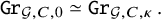 $$\begin{align*}\operatorname{\mathrm{\mathtt{Gr}}}_{\mathcal{G}, C, 0} \simeq \operatorname{\mathrm{\mathtt{Gr}}}_{\mathcal{G}, C, \kappa} .\end{align*}$$
Accordingly, the line bundle $\mathcal {L}_0$
can be translated to the level one line bundle
$\mathcal {L}_0$
can be translated to the level one line bundle $\mathcal {L}_\kappa $
on
$\mathcal {L}_\kappa $
on $\operatorname {\mathrm {\mathtt {Gr}}}_{\mathcal {G}, C, \kappa }$
. Note that given any two elements
$\operatorname {\mathrm {\mathtt {Gr}}}_{\mathcal {G}, C, \kappa }$
. Note that given any two elements $\kappa ,\kappa '\in M$
such that
$\kappa ,\kappa '\in M$
such that $\bar {\kappa }=\bar {\kappa '}$
in
$\bar {\kappa }=\bar {\kappa '}$
in $(X_*(T)/\check {Q})_\sigma $
,
$(X_*(T)/\check {Q})_\sigma $
, $\operatorname {\mathrm {\mathtt {Gr}}}_{\mathcal {G}, C, \kappa } $
and
$\operatorname {\mathrm {\mathtt {Gr}}}_{\mathcal {G}, C, \kappa } $
and $\operatorname {\mathrm {\mathtt {Gr}}}_{\mathcal {G}, C, \kappa '} $
share the same component
$\operatorname {\mathrm {\mathtt {Gr}}}_{\mathcal {G}, C, \kappa '} $
share the same component $\operatorname {\mathrm {\mathtt {Gr}}}_{{\mathscr {G}}, \bar {\kappa }}$
of
$\operatorname {\mathrm {\mathtt {Gr}}}_{{\mathscr {G}}, \bar {\kappa }}$
of $\operatorname {\mathrm {\mathtt {Gr}}}_{\mathscr {G}}$
at o and
$\operatorname {\mathrm {\mathtt {Gr}}}_{\mathscr {G}}$
at o and $\infty $
. Then
$\infty $
. Then $\mathcal {L}_\kappa $
and
$\mathcal {L}_\kappa $
and $\mathcal {L}_{\kappa '}$
agree on
$\mathcal {L}_{\kappa '}$
agree on $\operatorname {\mathrm {\mathtt {Gr}}}_{{\mathscr {G}}, \bar {\kappa }}$
as they have the same levels. Thus,
$\operatorname {\mathrm {\mathtt {Gr}}}_{{\mathscr {G}}, \bar {\kappa }}$
as they have the same levels. Thus, $\{ \mathcal {L}_\kappa \}_{\kappa \in M}$
glues to be a line bundle
$\{ \mathcal {L}_\kappa \}_{\kappa \in M}$
glues to be a line bundle $\mathcal {L}$
on
$\mathcal {L}$
on $\operatorname {\mathrm {\mathtt {Gr}}}_{\mathcal {G}, C}$
whose restriction to
$\operatorname {\mathrm {\mathtt {Gr}}}_{\mathcal {G}, C}$
whose restriction to $\operatorname {\mathrm {\mathtt {Gr}}}_{\mathcal {G}, p}$
is of level one, for any
$\operatorname {\mathrm {\mathtt {Gr}}}_{\mathcal {G}, p}$
is of level one, for any $p\in C$
.
$p\in C$
.
4 Smooth locus of twisted affine Schubert varieties
In this section, we always assume that $\sigma $
is a standard automorphism on G, and G is of adjoint type.
$\sigma $
is a standard automorphism on G, and G is of adjoint type.
4.1
$\operatorname {\mathrm {\mathtt {Gr}}}_{\mathscr {T}}$
as a fixed-point ind-subscheme of
$\operatorname {\mathrm {\mathtt {Gr}}}_{\mathscr {G}}$


We first recall a theorem in [Reference ZhuZh1, Theorem 1.3.4].
Theorem 4.1. The natural morphism $\operatorname {\mathrm {\mathtt {Gr}}}_{T} \rightarrow \operatorname {\mathrm {\mathtt {Gr}}}_{G}$
identifies
$\operatorname {\mathrm {\mathtt {Gr}}}_{T} \rightarrow \operatorname {\mathrm {\mathtt {Gr}}}_{G}$
identifies $\operatorname {\mathrm {\mathtt {Gr}}}_{T}$
as the T-fixed point ind-subscheme
$\operatorname {\mathrm {\mathtt {Gr}}}_{T}$
as the T-fixed point ind-subscheme $(\operatorname {\mathrm {\mathtt {Gr}}}_G)^T$
of
$(\operatorname {\mathrm {\mathtt {Gr}}}_G)^T$
of $\operatorname {\mathrm {\mathtt {Gr}}}_G$
.
$\operatorname {\mathrm {\mathtt {Gr}}}_G$
.
The original proof of this theorem is not correct (communicated to us by Richarz and Zhu independently); also, see [Reference Haines and RicharzHR2, Remark 3.5]. A correct proof can be found in [Reference Haines and RicharzHR2, Proposition 3.4], and a similar proof was known to Zhu earlier.
It is clear that $T^\sigma $
is a subgroup scheme of
$T^\sigma $
is a subgroup scheme of $L{\mathscr {T}}$
and
$L{\mathscr {T}}$
and $L{\mathscr {G}} $
. Hence, there is a natural action of
$L{\mathscr {G}} $
. Hence, there is a natural action of $T^\sigma $
on
$T^\sigma $
on $\operatorname {\mathrm {\mathtt {Gr}}}_{\mathscr {G}} $
. We now prove an analogue of Theorem 4.1 in the setting of special parahoric group schemes.
$\operatorname {\mathrm {\mathtt {Gr}}}_{\mathscr {G}} $
. We now prove an analogue of Theorem 4.1 in the setting of special parahoric group schemes.
Theorem 4.2. The natural morphism $ \operatorname {\mathrm {\mathtt {Gr}}}_{{\mathscr {T}} } \rightarrow \operatorname {\mathrm {\mathtt {Gr}}}_{{\mathscr {G}} }$
identifies
$ \operatorname {\mathrm {\mathtt {Gr}}}_{{\mathscr {T}} } \rightarrow \operatorname {\mathrm {\mathtt {Gr}}}_{{\mathscr {G}} }$
identifies $\operatorname {\mathrm {\mathtt {Gr}}}_{{\mathscr {T}} }$
as the
$\operatorname {\mathrm {\mathtt {Gr}}}_{{\mathscr {T}} }$
as the $T^\sigma $
-fixed point ind-subscheme
$T^\sigma $
-fixed point ind-subscheme $(\operatorname {\mathrm {\mathtt {Gr}}}_{\mathscr {G}} )^{T^\sigma }$
of
$(\operatorname {\mathrm {\mathtt {Gr}}}_{\mathscr {G}} )^{T^\sigma }$
of $\operatorname {\mathrm {\mathtt {Gr}}}_{\mathscr {G}} $
.
$\operatorname {\mathrm {\mathtt {Gr}}}_{\mathscr {G}} $
.
Proof. Let $L^{--}G$
be the ind-group scheme represented by the following functor, for any
$L^{--}G$
be the ind-group scheme represented by the following functor, for any $\mathbb {C}$
-algebra R,
$\mathbb {C}$
-algebra R,
 $$\begin{align*}L^{--}G(R): = \ker (\mathrm{ev}_{\infty}: G(R[t^{-1}]) \to G(R) ) , \end{align*}$$
where $\mathrm {ev}_{\infty }$
is the evaluation map sending
$\mathrm {ev}_{\infty }$
is the evaluation map sending $t^{-1}$
to
$t^{-1}$
to $0$
. Let
$0$
. Let $L^{--}{\mathscr {G}}$
be the ind-group scheme which represents the following functor, for any
$L^{--}{\mathscr {G}}$
be the ind-group scheme which represents the following functor, for any $\mathbb {C}$
-algebra R,
$\mathbb {C}$
-algebra R,
 $$ \begin{align} L^{--}{\mathscr{G}}(R): = \ker (\mathrm{ev}_{\infty}: G(R[t^{-1}])^\sigma \to G(R)^\sigma ). \end{align} $$
We can similarly define $L^{--}T$
and
$L^{--}T$
and $L^{--}{\mathscr {T}}$
.
$L^{--}{\mathscr {T}}$
.
By the similar argument as in [Reference ZhuZh4, Lemma 2.3.5] or [Reference Haines and RicharzHR2, Lemma 3.1], we have an open embedding
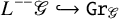 $$ \begin{align} L^{--}{\mathscr{G}}\hookrightarrow \operatorname{\mathrm{\mathtt{Gr}}}_{\mathscr{G}} \end{align} $$
given by $g\mapsto ge_0$
, where
$g\mapsto ge_0$
, where $e_0$
is the base point in
$e_0$
is the base point in $\operatorname {\mathrm {\mathtt {Gr}}}_{\mathscr {G}}$
. Let
$\operatorname {\mathrm {\mathtt {Gr}}}_{\mathscr {G}}$
. Let ${I}$
be the Iwahori subgroup of
${I}$
be the Iwahori subgroup of $L^+{\mathscr {G}}$
, which is the preimage of
$L^+{\mathscr {G}}$
, which is the preimage of $B^\sigma $
via the evaluation map
$B^\sigma $
via the evaluation map $\mathrm {ev}: L^+{\mathscr {G}}\to G^\sigma $
for a
$\mathrm {ev}: L^+{\mathscr {G}}\to G^\sigma $
for a $\sigma $
-stable Borel subgroup B in G. We have the following decomposition:
$\sigma $
-stable Borel subgroup B in G. We have the following decomposition:
 $$ \begin{align} \operatorname{\mathrm{\mathtt{Gr}}}_{\mathscr{G}}= \bigsqcup_{\bar{ \lambda} \in X_*(T)_\sigma } I e_{\bar{\lambda}}. \end{align} $$
For each $\bar {\lambda }\in X_*(T)_\sigma $
, we choose a representative
$\bar {\lambda }\in X_*(T)_\sigma $
, we choose a representative $\lambda \in X_*(T)$
. The twisted Iwahori Schubert cell
$\lambda \in X_*(T)$
. The twisted Iwahori Schubert cell
 $$\begin{align*}I e_{\bar{\lambda}}=n^{\lambda} \mathrm{Ad}_{ n^{-\lambda} } (I )e_0\end{align*}$$
is contained in $n^{\lambda } L^{--}{\mathscr {G}} e_0$
. Then by the decomposition (4.3),
$n^{\lambda } L^{--}{\mathscr {G}} e_0$
. Then by the decomposition (4.3), $\bigcup _{\bar {\lambda }\in X_*(T)_* } n^\lambda L^{--} {\mathscr {G}}e_0$
is an open covering of
$\bigcup _{\bar {\lambda }\in X_*(T)_* } n^\lambda L^{--} {\mathscr {G}}e_0$
is an open covering of $\operatorname {\mathrm {\mathtt {Gr}}}_{\mathscr {G}} $
. We may naturally regard
$\operatorname {\mathrm {\mathtt {Gr}}}_{\mathscr {G}} $
. We may naturally regard $\operatorname {\mathrm {\mathtt {Gr}}}_{\mathscr {T}}$
as an ind-subscheme of
$\operatorname {\mathrm {\mathtt {Gr}}}_{\mathscr {T}}$
as an ind-subscheme of $\operatorname {\mathrm {\mathtt {Gr}}}_{\mathscr {G}}$
. Hence, we may regard
$\operatorname {\mathrm {\mathtt {Gr}}}_{\mathscr {G}}$
. Hence, we may regard $e_0$
as the base point in
$e_0$
as the base point in $\operatorname {\mathrm {\mathtt {Gr}}}_{\mathscr {T}}$
. Under this convention,
$\operatorname {\mathrm {\mathtt {Gr}}}_{\mathscr {T}}$
. Under this convention,
 $$\begin{align*}\bigcup_{\lambda\in X_*(T)_\sigma} n^\lambda L^{--} {\mathscr{T}}e_0 = \bigcup_{\lambda\in X_*(T)_\sigma} L^{--} {\mathscr{T}} n^\lambda e_0 \end{align*}$$
is an open covering of $\operatorname {\mathrm {\mathtt {Gr}}}_{\mathscr {T}}$
. Therefore, it suffices to show that for each
$\operatorname {\mathrm {\mathtt {Gr}}}_{\mathscr {T}}$
. Therefore, it suffices to show that for each $\bar {\lambda }\in X_*(T)_\sigma $
,
$\bar {\lambda }\in X_*(T)_\sigma $
,
 $$\begin{align*}(n^\lambda L^{--} {\mathscr{G}}e_0)^{T^\sigma}\simeq n^\lambda L^{--} {\mathscr{T}}e_0. \end{align*}$$
Further, it suffices to show that $(L^{--} {\mathscr {G}})^{T^\sigma } \simeq L^{--}{\mathscr {T}}$
, where the action of
$(L^{--} {\mathscr {G}})^{T^\sigma } \simeq L^{--}{\mathscr {T}}$
, where the action of $T^\sigma $
on
$T^\sigma $
on $L^{--} {\mathscr {G}}$
is by conjugation. From the proof of [Reference Haines and RicharzHR2, Proposition 3.4], one may see that
$L^{--} {\mathscr {G}}$
is by conjugation. From the proof of [Reference Haines and RicharzHR2, Proposition 3.4], one may see that $(L^{--}G)^{T^\sigma }\simeq L^{--}T$
. This actually implies that
$(L^{--}G)^{T^\sigma }\simeq L^{--}T$
. This actually implies that $(L^{--} {\mathscr {G}})^{T^\sigma } \simeq L^{--}{\mathscr {T}}$
. Hence, this finishes the proof of the theorem.
$(L^{--} {\mathscr {G}})^{T^\sigma } \simeq L^{--}{\mathscr {T}}$
. Hence, this finishes the proof of the theorem.
An immediate consequence of Theorem 4.2 is the following corollary.
Corollary 4.3. The $T^\sigma $
-fixed
$T^\sigma $
-fixed $\mathbb {C}$
-point set in
$\mathbb {C}$
-point set in $\operatorname {\mathrm {\mathtt {Gr}}}_{\mathscr {G}} $
is
$\operatorname {\mathrm {\mathtt {Gr}}}_{\mathscr {G}} $
is $\{ e_{\bar {\lambda }} \,|\, \lambda \in X_*(T)_\sigma \}$
.
$\{ e_{\bar {\lambda }} \,|\, \lambda \in X_*(T)_\sigma \}$
.
4.2 A duality isomorphism for twisted Schubert varieties
Let $\operatorname {\mathrm {\mathtt {Gr}}}_G$
be the affine Grassmannian of G, and let
$\operatorname {\mathrm {\mathtt {Gr}}}_G$
be the affine Grassmannian of G, and let $\mathrm {L}$
be the line bundle on
$\mathrm {L}$
be the line bundle on $\operatorname {\mathrm {\mathtt {Gr}}}_G$
that is of level one on every component of
$\operatorname {\mathrm {\mathtt {Gr}}}_G$
that is of level one on every component of $\operatorname {\mathrm {\mathtt {Gr}}}_G$
. For any
$\operatorname {\mathrm {\mathtt {Gr}}}_G$
. For any $\lambda \in X_*(T)$
, let
$\lambda \in X_*(T)$
, let $\overline {\operatorname {\mathrm {\mathtt {Gr}}}}_G^\lambda $
denote the closure of
$\overline {\operatorname {\mathrm {\mathtt {Gr}}}}_G^\lambda $
denote the closure of $G(\mathcal {O})$
-orbit at
$G(\mathcal {O})$
-orbit at $L_\lambda :=t^\lambda G(\mathcal {O})\in \operatorname {\mathrm {\mathtt {Gr}}}_G$
. Let
$L_\lambda :=t^\lambda G(\mathcal {O})\in \operatorname {\mathrm {\mathtt {Gr}}}_G$
. Let $(\overline {\operatorname {\mathrm {\mathtt {Gr}}}}^\lambda _G)^T$
denote the T-fixed point subscheme of
$(\overline {\operatorname {\mathrm {\mathtt {Gr}}}}^\lambda _G)^T$
denote the T-fixed point subscheme of $\overline {\operatorname {\mathrm {\mathtt {Gr}}}}_G^\lambda $
. Zhu [Reference ZhuZh1, Theorem 0.2.2] proved the following.
$\overline {\operatorname {\mathrm {\mathtt {Gr}}}}_G^\lambda $
. Zhu [Reference ZhuZh1, Theorem 0.2.2] proved the following.
Theorem 4.4. When G is simply-laced and not of type E, the restriction map
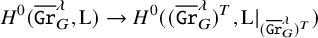 $$\begin{align*}H^0(\overline{\operatorname{\mathrm{\mathtt{Gr}}}}_{{G}}^{{\lambda}}, \mathrm{L}) \rightarrow H^0((\overline{\operatorname{\mathrm{\mathtt{Gr}}}}_{{G}}^{{\lambda}})^{T}, \mathrm{L}|_{(\overline{\operatorname{\mathrm{\mathtt{Gr}}}}_{ {G}}^{{\lambda}})^{T}}) \end{align*}$$
is an isomorphism.
In Section 5, we will show that this theorem also holds for $E_6$
. It was proved by Evens-Mirković [Reference Evens and MirkovićEM, Thereorem 0.1b] and Malkin-Ostrik-Vybornov [Reference Malkin, Ostrik and VybornovMOV, Corollary B] that the smooth locus of
$E_6$
. It was proved by Evens-Mirković [Reference Evens and MirkovićEM, Thereorem 0.1b] and Malkin-Ostrik-Vybornov [Reference Malkin, Ostrik and VybornovMOV, Corollary B] that the smooth locus of $\overline {\operatorname {\mathrm {\mathtt {Gr}}}}_G^\lambda $
is the open cell
$\overline {\operatorname {\mathrm {\mathtt {Gr}}}}_G^\lambda $
is the open cell $\operatorname {\mathrm {\mathtt {Gr}}}_G^\lambda $
for any reductive group G. In fact, this theorem can also be deduced from Theorem 4.4 in the simply- laced type.
$\operatorname {\mathrm {\mathtt {Gr}}}_G^\lambda $
for any reductive group G. In fact, this theorem can also be deduced from Theorem 4.4 in the simply- laced type.
We will prove a twisted version of Theorem 4.4 in full generality, and as a consequence we get the similar result of Evans-Mirković and Malkin-Ostrik-Vybornov in twisted setting. In particular, this confirms a conjecture of Haines-Richarz [Reference Haines and RicharzHR].
From Theorem 4.2, we have the identification $\operatorname {\mathrm {\mathtt {Gr}}}_{\mathscr {T}} \xrightarrow {\simeq } \operatorname {\mathrm {\mathtt {Gr}}}_{\mathscr {G}}^{T^{\sigma }}$
. Let
$\operatorname {\mathrm {\mathtt {Gr}}}_{\mathscr {T}} \xrightarrow {\simeq } \operatorname {\mathrm {\mathtt {Gr}}}_{\mathscr {G}}^{T^{\sigma }}$
. Let $\mathscr {I}^{\bar {\lambda }}$
denote the ideal sheaf of the
$\mathscr {I}^{\bar {\lambda }}$
denote the ideal sheaf of the $T^{\sigma }$
-fixed subscheme
$T^{\sigma }$
-fixed subscheme $(\overline {\operatorname {\mathrm {\mathtt {Gr}}}}_{\mathscr {G}}^{\bar {\lambda }})^{T^\sigma }$
of
$(\overline {\operatorname {\mathrm {\mathtt {Gr}}}}_{\mathscr {G}}^{\bar {\lambda }})^{T^\sigma }$
of $\overline {\operatorname {\mathrm {\mathtt {Gr}}}}_{\mathscr {G}}^{\bar {\lambda }}$
. Then we have a short exact sequence of sheaves
$\overline {\operatorname {\mathrm {\mathtt {Gr}}}}_{\mathscr {G}}^{\bar {\lambda }}$
. Then we have a short exact sequence of sheaves
 $$ \begin{align} 0 \rightarrow \mathscr{I}^{\bar{\lambda}} \rightarrow \mathscr{O}_{\overline{\operatorname{\mathrm{\mathtt{Gr}}}}_{\mathscr{G}}^{\bar{\lambda}}} \rightarrow \mathscr{O}_{(\overline{\operatorname{\mathrm{\mathtt{Gr}}}}_{\mathscr{G}}^{\bar{\lambda}})^{T^{\sigma}}} \rightarrow 0. \end{align} $$
Recall that $\mathscr {L}$
is the line bundle on
$\mathscr {L}$
is the line bundle on $\operatorname {\mathrm {\mathtt {Gr}}}_{\mathscr {G}}$
which is of level one on every component. Tensoring the above short exact sequence with
$\operatorname {\mathrm {\mathtt {Gr}}}_{\mathscr {G}}$
which is of level one on every component. Tensoring the above short exact sequence with $\mathscr {L}$
and taking the functor of global sections, we obtain the following exact sequence:
$\mathscr {L}$
and taking the functor of global sections, we obtain the following exact sequence:
 $$ \begin{align} \begin{aligned} 0 \rightarrow & H^0(\overline{\operatorname{\mathrm{\mathtt{Gr}}}}_{\mathscr{G}}^{\bar{\lambda}}, \mathscr{I}^{\bar{\lambda}}\otimes \mathscr{L} ) \rightarrow H^0(\overline{\operatorname{\mathrm{\mathtt{Gr}}}}_{\mathscr{G}}^{\bar{\lambda}}, \mathscr{L}) \xrightarrow{r} H^0((\overline{\operatorname{\mathrm{\mathtt{Gr}}}}_{\mathscr{G}}^{\bar{\lambda}})^{T^{\sigma}}, \mathscr{L}|_{(\overline{\operatorname{\mathrm{\mathtt{Gr}}}}_{\mathscr{G}}^{\bar{\lambda}})^{T^{\sigma}}}) \rightarrow \cdots, \end{aligned} \end{align} $$
where r is the restriction map.
Theorem 4.5. For any special parahoric group scheme ${\mathscr {G}}$
induced from a standard automorphism
${\mathscr {G}}$
induced from a standard automorphism $\sigma $
, the restriction map
$\sigma $
, the restriction map
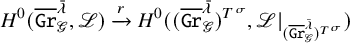 $$\begin{align*}H^0(\overline{\operatorname{\mathrm{\mathtt{Gr}}}}_{\mathscr{G}}^{\bar{\lambda}}, \mathscr{L}) \xrightarrow{r} H^0((\overline{\operatorname{\mathrm{\mathtt{Gr}}}}_{\mathscr{G}}^{\bar{\lambda}})^{T^{\sigma}}, \mathscr{L}|_{(\overline{\operatorname{\mathrm{\mathtt{Gr}}}}_{\mathscr{G}}^{\bar{\lambda}})^{T^{\sigma}}}) \end{align*}$$
is an isomorphism, where $\mathscr {L}$
is the level one line bundle on
$\mathscr {L}$
is the level one line bundle on $\operatorname {\mathrm {\mathtt {Gr}}}_{\mathscr {G}}$
.
$\operatorname {\mathrm {\mathtt {Gr}}}_{\mathscr {G}}$
.
This theorem will follow from the following proposition and Lemma 4.8.
Proposition 4.6. The map r is a surjection.
Proof. It is well known that any twisted affine Schubert variety $\overline {\operatorname {\mathrm {\mathtt {Gr}}}}_{\mathscr {G}}^{\bar {\lambda }}$
is a usual Schubert variety in a partial affine flag variety of Kac-Moody group. See the identification (3.11) and an argument for untwisted case in [Reference Besson and HongBH, Proposition 2.21]. By [Reference KumarKu, Theorem 8.2.2 (d)], we have that for any
$\overline {\operatorname {\mathrm {\mathtt {Gr}}}}_{\mathscr {G}}^{\bar {\lambda }}$
is a usual Schubert variety in a partial affine flag variety of Kac-Moody group. See the identification (3.11) and an argument for untwisted case in [Reference Besson and HongBH, Proposition 2.21]. By [Reference KumarKu, Theorem 8.2.2 (d)], we have that for any $\bar {\lambda } \succeq \bar {\mu }$
in
$\bar {\lambda } \succeq \bar {\mu }$
in $X_*(T)^+_\sigma $
, the following restriction map
$X_*(T)^+_\sigma $
, the following restriction map
 $$ \begin{align} H^0(\overline{\operatorname{\mathrm{\mathtt{Gr}}}}_{\mathscr{G}}^{\bar{\lambda}}, \mathscr{L}) \rightarrow H^0(\overline{\operatorname{\mathrm{\mathtt{Gr}}}}_{\mathscr{G}}^{\bar{\mu}}, \mathscr{L}) \end{align} $$
is surjective, and
 $$ \begin{align} H^0(\operatorname{\mathrm{\mathtt{Gr}}}_{\mathscr{G}}, \mathscr{L})= \varprojlim H^0(\overline{\operatorname{\mathrm{\mathtt{Gr}}}}^{\bar{\lambda}}_{\mathscr{G}}, \mathscr{L}|_{\overline{\operatorname{\mathrm{\mathtt{Gr}}}}^{\bar{\lambda}}_{\mathscr{G}}}). \end{align} $$
We also have the following surjective map
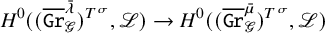 $$ \begin{align} H^0((\overline{\operatorname{\mathrm{\mathtt{Gr}}}}_{\mathscr{G}}^{\bar{\lambda}})^{T^{\sigma}}, \mathscr{L}) \rightarrow H^0((\overline{\operatorname{\mathrm{\mathtt{Gr}}}}_{\mathscr{G}}^{\bar{\mu}})^{T^{\sigma}}, \mathscr{L}) \end{align} $$
for all $\bar {\lambda } \succeq \bar {\mu }$
, since these
$\bar {\lambda } \succeq \bar {\mu }$
, since these $T^\sigma $
-fixed closed subschemes are affine and the morphism
$T^\sigma $
-fixed closed subschemes are affine and the morphism ![]() is a closed embedding. Moreover,
is a closed embedding. Moreover,
 $$\begin{align*}H^0((\operatorname{\mathrm{\mathtt{Gr}}}_{\mathscr{G}})^{T^\sigma} , \mathscr{L}|_{ (\operatorname{\mathrm{\mathtt{Gr}}}_{\mathscr{G}})^{T^\sigma} })= \varprojlim H^0((\overline{\operatorname{\mathrm{\mathtt{Gr}}}}^{\bar{\lambda}}_{{\mathscr{G}} })^{T^{\sigma}}, \mathscr{L}|_{(\overline{\operatorname{\mathrm{\mathtt{Gr}}}}^{\bar{\lambda}}_{\mathscr{G}})^{T^{\sigma}}}).\end{align*}$$
Therefore, for any $\bar {\lambda } \in X_*(T)^+_\sigma $
, we have the following surjective maps:
$\bar {\lambda } \in X_*(T)^+_\sigma $
, we have the following surjective maps:
 $$\begin{align*}H^0({\operatorname{\mathrm{\mathtt{Gr}}}}_{\mathscr{G}}, \mathscr{L}) \rightarrow H^0(\overline{\operatorname{\mathrm{\mathtt{Gr}}}}_{\mathscr{G}}^{\bar{\lambda}}, \mathscr{L}), \quad H^0(({\operatorname{\mathrm{\mathtt{Gr}}}}_{\mathscr{G}})^{T^{\sigma}}, \mathscr{L}) \rightarrow H^0((\overline{\operatorname{\mathrm{\mathtt{Gr}}}}_{\mathscr{G}}^{\bar{\lambda}})^{T^{\sigma}}, \mathscr{L}). \end{align*}$$
Then to prove the map
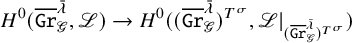 $$\begin{align*}H^0(\overline{\operatorname{\mathrm{\mathtt{Gr}}}}_{\mathscr{G}}^{\bar{\lambda}}, \mathscr{L}) \rightarrow H^0((\overline{\operatorname{\mathrm{\mathtt{Gr}}}}_{\mathscr{G}}^{\bar{\lambda}})^{T^{\sigma}}, \mathscr{L}|_{(\overline{\operatorname{\mathrm{\mathtt{Gr}}}}_{\mathscr{G}}^{\bar{\lambda}})^{T^{\sigma}}}) \end{align*}$$
is surjective, it is sufficient to prove that the map
 $$ \begin{align} H^0(\operatorname{\mathrm{\mathtt{Gr}}}_{\mathscr{G}}, \mathscr{L}) \rightarrow H^0( (\operatorname{\mathrm{\mathtt{Gr}}}_{\mathscr{G}})^{T^\sigma} , \mathscr{L}|_{ (\operatorname{\mathrm{\mathtt{Gr}}}_{\mathscr{G}})^{T^\sigma} }) \end{align} $$
is surjective, since we will have the following commutative diagram, for all $\bar {\lambda }$
:
$\bar {\lambda }$
:
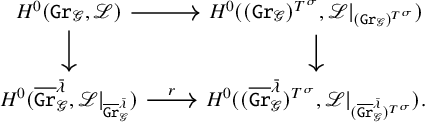
By Theorem 4.2, we have $\operatorname {\mathrm {\mathtt {Gr}}}_{\mathscr {T}}\simeq ( \operatorname {\mathrm {\mathtt {Gr}}}_{\mathscr {G}})^{T^\sigma } $
. Therefore, the surjectivity of the map (4.9) follows from the following Lemma 4.7.
$\operatorname {\mathrm {\mathtt {Gr}}}_{\mathscr {T}}\simeq ( \operatorname {\mathrm {\mathtt {Gr}}}_{\mathscr {G}})^{T^\sigma } $
. Therefore, the surjectivity of the map (4.9) follows from the following Lemma 4.7.
We first make a digression on Heisenberg algebras and their representations. Recall that $\mathfrak {h}$
is a fixed Cartan subalgebra in
$\mathfrak {h}$
is a fixed Cartan subalgebra in $\mathfrak {g}$
. The subspace
$\mathfrak {g}$
. The subspace $\hat {\mathfrak {h}}^{\sigma }:=( \mathfrak {h}_{\mathcal {K}})^{\sigma } \oplus \mathbb {C} K \hookrightarrow \hat {L}(\mathfrak {g}, \sigma )$
is a Lie subalgebra. In fact,
$\hat {\mathfrak {h}}^{\sigma }:=( \mathfrak {h}_{\mathcal {K}})^{\sigma } \oplus \mathbb {C} K \hookrightarrow \hat {L}(\mathfrak {g}, \sigma )$
is a Lie subalgebra. In fact, $\hat {\mathfrak {h}}^{\sigma }$
is an extended (completed) Heisenberg algebra with center
$\hat {\mathfrak {h}}^{\sigma }$
is an extended (completed) Heisenberg algebra with center $\mathfrak {h}^\sigma \oplus \mathbb {C} K$
. Therefore, any integrable irreducible highest weight representation of
$\mathfrak {h}^\sigma \oplus \mathbb {C} K$
. Therefore, any integrable irreducible highest weight representation of $\hat {\mathfrak {h}}^{\sigma }$
is parametrized by an element
$\hat {\mathfrak {h}}^{\sigma }$
is parametrized by an element $\mu \in (\mathfrak {h}^\sigma )^\vee $
and the level c (i.e., K acts by the scalar c on this representation). We denote this representation by
$\mu \in (\mathfrak {h}^\sigma )^\vee $
and the level c (i.e., K acts by the scalar c on this representation). We denote this representation by $ \pi _{\mu , c}$
. By the standard construction,
$ \pi _{\mu , c}$
. By the standard construction,
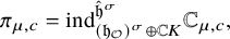 $$ \begin{align} \pi_{\mu, c}=\mathrm{ind}_{(\mathfrak{h}_{\mathcal{O}})^\sigma\oplus \mathbb{C} K }^{\hat{\mathfrak{h}}^{\sigma}} \mathbb{C}_{\mu, c} ,\end{align} $$
where $\mathrm {ind}$
is the induced representation in the sense of universal enveloping algebras, and
$\mathrm {ind}$
is the induced representation in the sense of universal enveloping algebras, and $ \mathbb {C}_{\mu , c}$
is the 1-dimensional module over
$ \mathbb {C}_{\mu , c}$
is the 1-dimensional module over $(\mathfrak {h}_{O})^\sigma \oplus \mathbb {C} K$
where the action of
$(\mathfrak {h}_{O})^\sigma \oplus \mathbb {C} K$
where the action of $(\mathfrak {h}_{O})^\sigma $
factors through
$(\mathfrak {h}_{O})^\sigma $
factors through $\mathfrak {h}^\sigma $
.
$\mathfrak {h}^\sigma $
.
Lemma 4.7. The restriction map $H^0(\operatorname {\mathrm {\mathtt {Gr}}}_{\mathscr {G}}, \mathscr {L}^c ) \rightarrow H^0(\operatorname {\mathrm {\mathtt {Gr}}}_{\mathscr {T}}, \mathscr {L}^c |_{ \operatorname {\mathrm {\mathtt {Gr}}}_{\mathscr {T}} })$
is surjective.
$H^0(\operatorname {\mathrm {\mathtt {Gr}}}_{\mathscr {G}}, \mathscr {L}^c ) \rightarrow H^0(\operatorname {\mathrm {\mathtt {Gr}}}_{\mathscr {T}}, \mathscr {L}^c |_{ \operatorname {\mathrm {\mathtt {Gr}}}_{\mathscr {T}} })$
is surjective.
Proof. Proving surjectivity here is equivalent to proving injectivity for the dual modules,
 $$\begin{align*}0 \rightarrow H^0(\operatorname{\mathrm{\mathtt{Gr}}}_{\mathscr{T}}, \mathscr{L}^c|_{\operatorname{\mathrm{\mathtt{Gr}}}_{\mathscr{T}}})^\vee \rightarrow H^0(\operatorname{\mathrm{\mathtt{Gr}}}_{\mathscr{G}}, \mathscr{L}^c)^\vee. \end{align*}$$
Note that both of these spaces are modules for the Heisenberg algebra $\hat {\mathfrak {h}}^{\sigma }$
; the morphism is a
$\hat {\mathfrak {h}}^{\sigma }$
; the morphism is a $\hat {\mathfrak {h}}^{\sigma }$
-morphism. Since
$\hat {\mathfrak {h}}^{\sigma }$
-morphism. Since ${\mathscr {T}}$
is discrete, we naturally have the following decomposition:
${\mathscr {T}}$
is discrete, we naturally have the following decomposition:
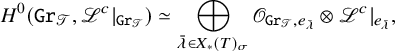 $$\begin{align*}H^0(\operatorname{\mathrm{\mathtt{Gr}}}_{\mathscr{T}}, \mathscr{L}^c|_{\operatorname{\mathrm{\mathtt{Gr}}}_{\mathscr{T}}})\simeq \bigoplus_{\bar{\lambda} \in X_*(T)_\sigma } \mathscr{O}_{ \operatorname{\mathrm{\mathtt{Gr}}}_{\mathscr{T}}, e_{\bar{\lambda}} }\otimes \mathscr{L}^c|_{ e_{\bar{\lambda} } }, \end{align*}$$
where $\mathscr {O}_{ \operatorname {\mathrm {\mathtt {Gr}}}_{\mathscr {T}}, e_{\bar {\lambda }} }$
is the structure sheaf of the component of
$\mathscr {O}_{ \operatorname {\mathrm {\mathtt {Gr}}}_{\mathscr {T}}, e_{\bar {\lambda }} }$
is the structure sheaf of the component of $\operatorname {\mathrm {\mathtt {Gr}}}_{\mathscr {T}}$
containing
$\operatorname {\mathrm {\mathtt {Gr}}}_{\mathscr {T}}$
containing $e_{\bar {\lambda }}$
. We also notice that the identity component of
$e_{\bar {\lambda }}$
. We also notice that the identity component of $\operatorname {\mathrm {\mathtt {Gr}}}_{\mathscr {T}}$
is naturally the formal group with Lie algebra
$\operatorname {\mathrm {\mathtt {Gr}}}_{\mathscr {T}}$
is naturally the formal group with Lie algebra $(\mathfrak {h}_{\mathcal {K}})^\sigma /(\mathfrak {h}_{\mathcal {O}})^\sigma $
. In view of the construction (4.11), we have
$(\mathfrak {h}_{\mathcal {K}})^\sigma /(\mathfrak {h}_{\mathcal {O}})^\sigma $
. In view of the construction (4.11), we have
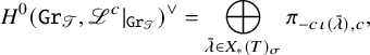 $$\begin{align*}H^0(\operatorname{\mathrm{\mathtt{Gr}}}_{\mathscr{T}}, \mathscr{L}^c|_{\operatorname{\mathrm{\mathtt{Gr}}}_{\mathscr{T}}})^\vee= \bigoplus_{\bar{\lambda} \in X_*(T)_\sigma } \pi_{-c\iota(\bar{\lambda}) , c },\end{align*}$$
where the map $\iota : X_*(T)_{\sigma } \rightarrow (\mathfrak {h}^\sigma )^\vee $
is defined in (3.2). Since each
$\iota : X_*(T)_{\sigma } \rightarrow (\mathfrak {h}^\sigma )^\vee $
is defined in (3.2). Since each $\pi _{-c\iota (\bar {\lambda }) , c }$
is irreducible, and generated by a
$\pi _{-c\iota (\bar {\lambda }) , c }$
is irreducible, and generated by a $-c\iota (\bar {\lambda })$
-weight vector
$-c\iota (\bar {\lambda })$
-weight vector $w_{-c\iota (\bar {\lambda })}$
, it suffices to show that the morphism
$w_{-c\iota (\bar {\lambda })}$
, it suffices to show that the morphism
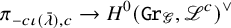 $$\begin{align*}\pi_{-c\iota(\bar{\lambda}) , c } \rightarrow H^0(\operatorname{\mathrm{\mathtt{Gr}}}_{\mathscr{G}}, \mathscr{L}^c)^\vee\end{align*}$$
sends $w_{-c\iota (\bar {\lambda })}$
to a nonzero vector.
$w_{-c\iota (\bar {\lambda })}$
to a nonzero vector.
By Theorem 3.8, we may define a Plücker embedding
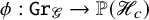 $$\begin{align*}\phi: \operatorname{\mathrm{\mathtt{Gr}}}_{\mathscr{G}} \rightarrow \mathbb{P}( \mathscr{H}_c )\end{align*}$$
given by $ge_0\mapsto [\rho _g ( v_0 )]$
for any
$ge_0\mapsto [\rho _g ( v_0 )]$
for any $ge_0\in \operatorname {\mathrm {\mathtt {Gr}}}_{\mathscr {G}} $
, where
$ge_0\in \operatorname {\mathrm {\mathtt {Gr}}}_{\mathscr {G}} $
, where $\rho _g$
is defined in Lemma 3.6, and
$\rho _g$
is defined in Lemma 3.6, and $ [\rho _g ( v_0) ]$
represents the line in
$ [\rho _g ( v_0) ]$
represents the line in $\mathscr {H}_c $
that contains
$\mathscr {H}_c $
that contains $ \rho _g ( v_0) $
, where
$ \rho _g ( v_0) $
, where $v_0$
is the highest weight vector in
$v_0$
is the highest weight vector in $\mathscr {H}_c$
. Then we may pick a linear form
$\mathscr {H}_c$
. Then we may pick a linear form $f_{\bar {\lambda }}$
on
$f_{\bar {\lambda }}$
on $\mathscr {H}_c$
which is nonzero on the line
$\mathscr {H}_c$
which is nonzero on the line $[v_{\bar {\lambda }}]$
containing the extremal weight vector
$[v_{\bar {\lambda }}]$
containing the extremal weight vector $v_{\bar {\lambda }}$
, and which is 0 on other weight vectors, where
$v_{\bar {\lambda }}$
, and which is 0 on other weight vectors, where $v_{\bar {\lambda }}$
is defined in (3.15). The restriction
$v_{\bar {\lambda }}$
is defined in (3.15). The restriction $f_{\bar {\lambda }}|_{\phi (\operatorname {\mathrm {\mathtt {Gr}}}_{\mathscr {G}})}$
produces a nontrivial element in
$f_{\bar {\lambda }}|_{\phi (\operatorname {\mathrm {\mathtt {Gr}}}_{\mathscr {G}})}$
produces a nontrivial element in $H^0(\operatorname {\mathrm {\mathtt {Gr}}}_{\mathscr {G}}, \mathscr {L})$
, since
$H^0(\operatorname {\mathrm {\mathtt {Gr}}}_{\mathscr {G}}, \mathscr {L})$
, since $\phi (e_{\bar {\lambda }})=v_{\bar {\lambda }}$
.
$\phi (e_{\bar {\lambda }})=v_{\bar {\lambda }}$
.
Observe that the map $ \pi _{-c\iota (\bar {\lambda }) , c } \rightarrow H^0(\operatorname {\mathrm {\mathtt {Gr}}}_{\mathscr {G}}, \mathscr {L}^c)^\vee $
sends
$ \pi _{-c\iota (\bar {\lambda }) , c } \rightarrow H^0(\operatorname {\mathrm {\mathtt {Gr}}}_{\mathscr {G}}, \mathscr {L}^c)^\vee $
sends $w_{-c\iota (\bar {\lambda })}$
to a nonzero scalar of
$w_{-c\iota (\bar {\lambda })}$
to a nonzero scalar of $v_{\bar {\lambda } }$
. Thus, the map
$v_{\bar {\lambda } }$
. Thus, the map $ \pi _{-c\iota (\bar {\lambda }) , c } \rightarrow H^0(\operatorname {\mathrm {\mathtt {Gr}}}_{\mathscr {G}}, \mathscr {L}^c)^\vee $
is nontrivial and thus injective.
$ \pi _{-c\iota (\bar {\lambda }) , c } \rightarrow H^0(\operatorname {\mathrm {\mathtt {Gr}}}_{\mathscr {G}}, \mathscr {L}^c)^\vee $
is nontrivial and thus injective.
By Lemma 4.7, we obtain the following short exact sequence:
 $$\begin{align*}0 \rightarrow H^0(\overline{\operatorname{\mathrm{\mathtt{Gr}}}}_{\mathscr{G}}^{\bar{\lambda}}, \mathscr{I}^{\bar{\lambda}}\otimes \mathscr{L}) \rightarrow H^0(\overline{\operatorname{\mathrm{\mathtt{Gr}}}}_{\mathscr{G}}^{\bar{\lambda}}, \mathscr{L}) \xrightarrow{r} H^0(\overline{\operatorname{\mathrm{\mathtt{Gr}}}}_{\mathscr{G}}^{\bar{\lambda}}, \mathscr{L} \otimes \mathscr{O}_{(\overline{\operatorname{\mathrm{\mathtt{Gr}}}}_{\mathscr{G}}^{\bar{\lambda}})}) \rightarrow 0.\end{align*}$$
Thus, the obstruction to the map r being an isomorphism is the vanishing of the first term $ H^0(\overline {\operatorname {\mathrm {\mathtt {Gr}}}}_{\mathscr {G}}^{\bar {\lambda }}, \mathscr {I}^{\bar {\lambda }} \otimes \mathscr {L} )$
.
$ H^0(\overline {\operatorname {\mathrm {\mathtt {Gr}}}}_{\mathscr {G}}^{\bar {\lambda }}, \mathscr {I}^{\bar {\lambda }} \otimes \mathscr {L} )$
.
Let $\mathrm {I}^{\lambda }$
denote the ideal sheaf of the T-fixed subscheme on
$\mathrm {I}^{\lambda }$
denote the ideal sheaf of the T-fixed subscheme on $\overline {\operatorname {\mathrm {\mathtt {Gr}}}}_G^{\lambda }$
. We will show that the vanishing of the first term can be deduced from the vanishing of
$\overline {\operatorname {\mathrm {\mathtt {Gr}}}}_G^{\lambda }$
. We will show that the vanishing of the first term can be deduced from the vanishing of $H^0(\overline {\operatorname {\mathrm {\mathtt {Gr}}}}_G^{\lambda }, \mathrm {I}^{\lambda } \otimes \mathrm {L})$
.
$H^0(\overline {\operatorname {\mathrm {\mathtt {Gr}}}}_G^{\lambda }, \mathrm {I}^{\lambda } \otimes \mathrm {L})$
.
Recall that $\overline {\operatorname {\mathrm {\mathtt {Gr}}}}_{\mathcal {G}, C}^{\lambda }$
is a global Schubert variety defined in Section 2.5. The constant group scheme
$\overline {\operatorname {\mathrm {\mathtt {Gr}}}}_{\mathcal {G}, C}^{\lambda }$
is a global Schubert variety defined in Section 2.5. The constant group scheme $T^\sigma \times C$
over C is naturally a closed subgroup scheme of
$T^\sigma \times C$
over C is naturally a closed subgroup scheme of $\mathcal {T}$
. Hence,
$\mathcal {T}$
. Hence, $T^\sigma $
acts on
$T^\sigma $
acts on $\overline {\operatorname {\mathrm {\mathtt {Gr}}}}_{\mathcal {G}, C}^{\lambda }$
naturally. Let
$\overline {\operatorname {\mathrm {\mathtt {Gr}}}}_{\mathcal {G}, C}^{\lambda }$
naturally. Let $(\overline {\operatorname {\mathrm {\mathtt {Gr}}}}_{\mathcal {G}, C}^{\lambda })^{T^\sigma }$
be the
$(\overline {\operatorname {\mathrm {\mathtt {Gr}}}}_{\mathcal {G}, C}^{\lambda })^{T^\sigma }$
be the $T^\sigma $
-fixed subscheme of
$T^\sigma $
-fixed subscheme of $\overline {\operatorname {\mathrm {\mathtt {Gr}}}}_{\mathcal {G}, C}^{\lambda }$
, and let
$\overline {\operatorname {\mathrm {\mathtt {Gr}}}}_{\mathcal {G}, C}^{\lambda }$
, and let $\mathcal {I}^{\lambda }$
be the ideal sheaf of
$\mathcal {I}^{\lambda }$
be the ideal sheaf of $(\overline {\operatorname {\mathrm {\mathtt {Gr}}}}_{\mathcal {G}, C}^{\lambda })^{T^\sigma }$
. Then,
$(\overline {\operatorname {\mathrm {\mathtt {Gr}}}}_{\mathcal {G}, C}^{\lambda })^{T^\sigma }$
. Then, $\mathcal {I}^\lambda |_p$
is the ideal sheaf of
$\mathcal {I}^\lambda |_p$
is the ideal sheaf of $(\overline {\operatorname {\mathrm {\mathtt {Gr}}}}_{\mathcal {G}, C}^{\lambda }|_{p})^{T^\sigma }$
. Recall that
$(\overline {\operatorname {\mathrm {\mathtt {Gr}}}}_{\mathcal {G}, C}^{\lambda }|_{p})^{T^\sigma }$
. Recall that
 $$\begin{align*}\overline{\operatorname{\mathrm{\mathtt{Gr}}}}_{ {\mathcal{G}},o}^{\lambda} = \overline{\operatorname{\mathrm{\mathtt{Gr}}}}_{\mathscr{G}}^{\bar{\lambda}}, \quad \overline{\operatorname{\mathrm{\mathtt{Gr}}}}_{ {\mathcal{G}},\infty}^{\lambda}\simeq \overline{\operatorname{\mathrm{\mathtt{Gr}}}}_{\mathscr{G}}^{\bar{\lambda}}, \quad \overline{\operatorname{\mathrm{\mathtt{Gr}}}}_{\mathcal{G},p \neq o,\infty }^{\lambda} \simeq \overline{\operatorname{\mathrm{\mathtt{Gr}}}}_{G}^{\lambda}.\end{align*}$$
In particular, we have
 $$\begin{align*}\mathcal{I}^\lambda|_o= \mathscr{I}^\lambda, \quad \mathcal{I}^\lambda|_\infty\simeq \mathscr{I}^\lambda, \quad \mathcal{I}^\lambda|_{p\not= o,\infty}\simeq \mathrm{I}^\lambda.\end{align*}$$
Lemma 4.8. The ideal $\mathcal {I}^\lambda $
is flat over C.
$\mathcal {I}^\lambda $
is flat over C.
Proof. Consider $\overline {\operatorname {\mathrm {\mathtt {Gr}}}}_{\mathcal {G}, {C} \setminus \{o,\infty \}}^{\lambda }$
and the
$\overline {\operatorname {\mathrm {\mathtt {Gr}}}}_{\mathcal {G}, {C} \setminus \{o,\infty \}}^{\lambda }$
and the $T^{\sigma }$
-fixed subscheme
$T^{\sigma }$
-fixed subscheme $(\overline {\operatorname {\mathrm {\mathtt {Gr}}}}_{\mathcal {G}, {C} \setminus \{ o,\infty \}}^{\lambda })^{T^{\sigma }}$
. We denote by
$(\overline {\operatorname {\mathrm {\mathtt {Gr}}}}_{\mathcal {G}, {C} \setminus \{ o,\infty \}}^{\lambda })^{T^{\sigma }}$
. We denote by $Z^{\lambda }$
the flat closure of
$Z^{\lambda }$
the flat closure of $(\overline {\operatorname {\mathrm {\mathtt {Gr}}}}_{\mathcal {G}, C \setminus \{o,\infty \}}^{\lambda })^{T^{\sigma }}$
in
$(\overline {\operatorname {\mathrm {\mathtt {Gr}}}}_{\mathcal {G}, C \setminus \{o,\infty \}}^{\lambda })^{T^{\sigma }}$
in $\operatorname {\mathrm {\mathtt {Gr}}}_{\mathcal {G}, C}$
. Since Z is the closure of a
$\operatorname {\mathrm {\mathtt {Gr}}}_{\mathcal {G}, C}$
. Since Z is the closure of a $T^{\sigma }$
-fixed subscheme, we see that
$T^{\sigma }$
-fixed subscheme, we see that $Z^{\lambda }|_o \subset \overline {\operatorname {\mathrm {\mathtt {Gr}}}}^{\lambda }_{\mathcal {G}, C}|_o$
, and
$Z^{\lambda }|_o \subset \overline {\operatorname {\mathrm {\mathtt {Gr}}}}^{\lambda }_{\mathcal {G}, C}|_o$
, and $Z^{\lambda }|_\infty \subset \overline {\operatorname {\mathrm {\mathtt {Gr}}}}^{\lambda }_{\mathcal {G}, C}|_\infty .$
To show $\mathcal {I}^\lambda $
is flat over C, it is sufficient to show that
$\mathcal {I}^\lambda $
is flat over C, it is sufficient to show that $(\overline {\operatorname {\mathrm {\mathtt {Gr}}}}_{\mathcal {G}, C}^{\lambda })^{T^\sigma }$
is flat over C. This is equivalent to showing
$(\overline {\operatorname {\mathrm {\mathtt {Gr}}}}_{\mathcal {G}, C}^{\lambda })^{T^\sigma }$
is flat over C. This is equivalent to showing $Z^\lambda =(\overline {\operatorname {\mathrm {\mathtt {Gr}}}}_{\mathcal {G}, C}^{\lambda })^{T^\sigma }$
. In particular, it suffices to show the fibers
$Z^\lambda =(\overline {\operatorname {\mathrm {\mathtt {Gr}}}}_{\mathcal {G}, C}^{\lambda })^{T^\sigma }$
. In particular, it suffices to show the fibers $Z^{\lambda }|_o$
and
$Z^{\lambda }|_o$
and $Z^{\lambda }|_\infty $
are isomorphic to
$Z^{\lambda }|_\infty $
are isomorphic to $(\overline {\operatorname {\mathrm {\mathtt {Gr}}}}_{\mathscr {G}}^{\bar {\lambda }})^{T^{\sigma }}$
. Since the fiber
$(\overline {\operatorname {\mathrm {\mathtt {Gr}}}}_{\mathscr {G}}^{\bar {\lambda }})^{T^{\sigma }}$
. Since the fiber $Z^{\lambda }|_\infty $
at
$Z^{\lambda }|_\infty $
at $\infty $
is similar to the fiber
$\infty $
is similar to the fiber $Z^{\lambda }|_o$
at o, it suffices to show that
$Z^{\lambda }|_o$
at o, it suffices to show that $Z^{\lambda }|_o=(\overline {\operatorname {\mathrm {\mathtt {Gr}}}}_{\mathscr {G}}^{\bar {\lambda }})^{T^{\sigma }}$
. Note that both of these are finite schemes; we can compare the dimensions of their structure sheaves as follows:
$Z^{\lambda }|_o=(\overline {\operatorname {\mathrm {\mathtt {Gr}}}}_{\mathscr {G}}^{\bar {\lambda }})^{T^{\sigma }}$
. Note that both of these are finite schemes; we can compare the dimensions of their structure sheaves as follows:
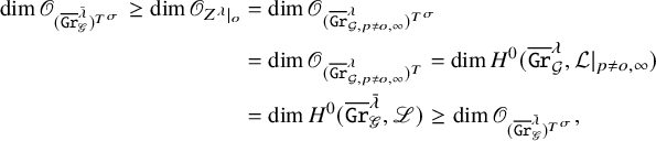 $$ \begin{align*} \dim \mathscr{O}_{(\overline{\operatorname{\mathrm{\mathtt{Gr}}}}_{{\mathscr{G}} }^{\bar{\lambda}})^{T^{\sigma}}} \geq \dim \mathscr{O}_{Z^{\lambda}|_o} &= \dim \mathscr{O}_{(\overline{\operatorname{\mathrm{\mathtt{Gr}}}}_{\mathcal{G},p \neq o ,\infty}^{\lambda} )^{T^\sigma}} \\ & = \dim \mathscr{O}_{(\overline{\operatorname{\mathrm{\mathtt{Gr}}}}_{\mathcal{G},p \neq o,\infty }^{\lambda} )^{T}} = \dim H^0( \overline{\operatorname{\mathrm{\mathtt{Gr}}}}_{\mathcal{G}}^{\lambda}, \mathcal{L}|_{p\neq o,\infty} ) \\ & = \dim H^0(\overline{\operatorname{\mathrm{\mathtt{Gr}}}}_{\mathscr{G}}^{\bar{\lambda}}, \mathscr{L}) \geq \dim \mathscr{O}_{(\overline{\operatorname{\mathrm{\mathtt{Gr}}}}_{{\mathscr{G}} }^{\bar{\lambda}})^{T^{\sigma}}}, \end{align*} $$
where the first equality follows from the flatness of $Z^\lambda $
over C, the third equality follows from Theorem 4.4 and Theorem 5.1, the fourth equality follows since
$Z^\lambda $
over C, the third equality follows from Theorem 4.4 and Theorem 5.1, the fourth equality follows since $\overline {\operatorname {\mathrm {\mathtt {Gr}}}}_{\mathcal {G},C}^{{\lambda }}$
is flat over C (cf. Theorem 2.4), and the last inequality follows from Proposition 4.6. From this comparison, it follows that
$\overline {\operatorname {\mathrm {\mathtt {Gr}}}}_{\mathcal {G},C}^{{\lambda }}$
is flat over C (cf. Theorem 2.4), and the last inequality follows from Proposition 4.6. From this comparison, it follows that $\dim \mathscr {O}_{Z^{\lambda }|_o} = \dim \mathscr {O}_{(\overline {\operatorname {\mathrm {\mathtt {Gr}}}}_{\mathcal {G},p \neq o }^{\lambda } )^{T^\sigma }}$
. Hence,
$\dim \mathscr {O}_{Z^{\lambda }|_o} = \dim \mathscr {O}_{(\overline {\operatorname {\mathrm {\mathtt {Gr}}}}_{\mathcal {G},p \neq o }^{\lambda } )^{T^\sigma }}$
. Hence, $\mathscr {O}_{Z^{\lambda }|_o} = \mathscr {O}_{(\overline {\operatorname {\mathrm {\mathtt {Gr}}}}_{\mathcal {G},p \neq 0 }^{\lambda } )^{T^\sigma }}$
. This concludes the proof of the lemma.
$\mathscr {O}_{Z^{\lambda }|_o} = \mathscr {O}_{(\overline {\operatorname {\mathrm {\mathtt {Gr}}}}_{\mathcal {G},p \neq 0 }^{\lambda } )^{T^\sigma }}$
. This concludes the proof of the lemma.
Proof of Theorem 4.5.
By Lemma 4.8 and the properness of $\overline {\operatorname {\mathrm {\mathtt {Gr}}}}_{\mathcal {G}, C}^{\lambda }$
over C, we have
$\overline {\operatorname {\mathrm {\mathtt {Gr}}}}_{\mathcal {G}, C}^{\lambda }$
over C, we have
 $$ \begin{align} \sum_{i\geq 0} (-1)^i \dim H^i(\overline{\operatorname{\mathrm{\mathtt{Gr}}}}_{G}^{\lambda}, \mathrm{I}^{\lambda} \otimes \mathrm{L})=\sum_{i\geq 0} (-1)^i \dim H^i(\overline{\operatorname{\mathrm{\mathtt{Gr}}}}_{\mathscr{G}} ^{\bar{\lambda}}, \mathscr{I}^{\bar{\lambda}} \otimes \mathscr{L}). \end{align} $$
By [Reference Pappas and RapoportPR, 9.h.] and [Reference KumarKu, Theorem 8.2.2], we have $H^i(\overline {\operatorname {\mathrm {\mathtt {Gr}}}}_{G}^{\lambda }, \mathrm {L})=0$
and
$H^i(\overline {\operatorname {\mathrm {\mathtt {Gr}}}}_{G}^{\lambda }, \mathrm {L})=0$
and $H^i(\overline {\operatorname {\mathrm {\mathtt {Gr}}}}_{\mathscr {G}} ^{\bar {\lambda }}, \mathscr {L})=0 $
for any
$H^i(\overline {\operatorname {\mathrm {\mathtt {Gr}}}}_{\mathscr {G}} ^{\bar {\lambda }}, \mathscr {L})=0 $
for any $i>0$
. From [Reference ZhuZh1, Section 2.2] when G is of type A and D and from Section 5 when G is of type
$i>0$
. From [Reference ZhuZh1, Section 2.2] when G is of type A and D and from Section 5 when G is of type $E_6$
, we have the following vanishing
$E_6$
, we have the following vanishing $H^i(\overline {\operatorname {\mathrm {\mathtt {Gr}}}}_{G}^{\lambda }, \mathrm {I}^{\lambda } \otimes \mathrm {L})=0$
for any
$H^i(\overline {\operatorname {\mathrm {\mathtt {Gr}}}}_{G}^{\lambda }, \mathrm {I}^{\lambda } \otimes \mathrm {L})=0$
for any $\lambda \in X_*(T)^+$
, by considering the exact sequence (4.5) in the untwisted case. From Lemma 4.7 and the long exact sequence (4.5), we can see easily that
$\lambda \in X_*(T)^+$
, by considering the exact sequence (4.5) in the untwisted case. From Lemma 4.7 and the long exact sequence (4.5), we can see easily that $H^i(\overline {\operatorname {\mathrm {\mathtt {Gr}}}}_{\mathscr {G}} ^{\bar {\lambda }}, \mathscr {I}^{\bar {\lambda }} \otimes \mathscr {L})=0$
for any
$H^i(\overline {\operatorname {\mathrm {\mathtt {Gr}}}}_{\mathscr {G}} ^{\bar {\lambda }}, \mathscr {I}^{\bar {\lambda }} \otimes \mathscr {L})=0$
for any $i\geq 1$
. Hence, the equality (4.12) implies that
$i\geq 1$
. Hence, the equality (4.12) implies that $H^0(\overline {\operatorname {\mathrm {\mathtt {Gr}}}}_{\mathscr {G}} ^{\bar {\lambda }}, \mathscr {I}^{\bar {\lambda }} \otimes \mathscr {L})=0$
for any
$H^0(\overline {\operatorname {\mathrm {\mathtt {Gr}}}}_{\mathscr {G}} ^{\bar {\lambda }}, \mathscr {I}^{\bar {\lambda }} \otimes \mathscr {L})=0$
for any $\bar {\lambda }\in X_*(T)^+_\sigma $
. Therefore, the theorem finally follows from the long exact sequence (4.5).
$\bar {\lambda }\in X_*(T)^+_\sigma $
. Therefore, the theorem finally follows from the long exact sequence (4.5).
As an application of Theorem 4.5, we get a geometric Frenkel-Kac isomorphism for twisted affine algebras.
Theorem 4.9. For any special parahoric group scheme ${\mathscr {G}}$
induced from a standard automorphism
${\mathscr {G}}$
induced from a standard automorphism $\sigma $
, the restriction map
$\sigma $
, the restriction map
 $$\begin{align*}H^0(\operatorname{\mathrm{\mathtt{Gr}}}_{\mathscr{G}}, \mathscr{L} ) \rightarrow H^0(\operatorname{\mathrm{\mathtt{Gr}}}_{\mathscr{T}}, \mathscr{L}|_{ \operatorname{\mathrm{\mathtt{Gr}}}_{\mathscr{T}} })\end{align*}$$
is an isomoprhism, via the embedding $\operatorname {\mathrm {\mathtt {Gr}}}_{\mathscr {T}}\to \operatorname {\mathrm {\mathtt {Gr}}}_{\mathscr {G}}$
.
$\operatorname {\mathrm {\mathtt {Gr}}}_{\mathscr {T}}\to \operatorname {\mathrm {\mathtt {Gr}}}_{\mathscr {G}}$
.
Proof. By Theorem 4.2, it suffices to show that the restriction map $r:H^0(\operatorname {\mathrm {\mathtt {Gr}}}_{\mathscr {G}}, \mathscr {L} ) \rightarrow H^0(\operatorname {\mathrm {\mathtt {Gr}}}_{\mathscr {T}}, \mathscr {L}|_{( \operatorname {\mathrm {\mathtt {Gr}}}_{{\mathscr {G}} })^{T^\sigma } }) $
is an isomorphism. In view of (4.7) and (4.8) and as a consequence of Theorem 4.5, the restriction map r is an isomorphism.
$r:H^0(\operatorname {\mathrm {\mathtt {Gr}}}_{\mathscr {G}}, \mathscr {L} ) \rightarrow H^0(\operatorname {\mathrm {\mathtt {Gr}}}_{\mathscr {T}}, \mathscr {L}|_{( \operatorname {\mathrm {\mathtt {Gr}}}_{{\mathscr {G}} })^{T^\sigma } }) $
is an isomorphism. In view of (4.7) and (4.8) and as a consequence of Theorem 4.5, the restriction map r is an isomorphism.
4.3 Application: smooth locus of twisted affine Schubert varieties
We now wish to investigate the smooth locus of the Schubert variety $\overline {\operatorname {\mathrm {\mathtt {Gr}}}}_{{\mathscr {G}} }^{\bar {\lambda }}$
.
$\overline {\operatorname {\mathrm {\mathtt {Gr}}}}_{{\mathscr {G}} }^{\bar {\lambda }}$
.
Theorem 4.10. Assume that ${\mathscr {G}}$
is not of type
${\mathscr {G}}$
is not of type $A_{2\ell }^{(2)}$
. For any
$A_{2\ell }^{(2)}$
. For any $\lambda \in X_*(T)_\sigma ^+$
, the smooth locus of
$\lambda \in X_*(T)_\sigma ^+$
, the smooth locus of $\overline {\operatorname {\mathrm {\mathtt {Gr}}}}_{{\mathscr {G}} }^{\bar {\lambda }}$
is precisely the open Schubert cell
$\overline {\operatorname {\mathrm {\mathtt {Gr}}}}_{{\mathscr {G}} }^{\bar {\lambda }}$
is precisely the open Schubert cell $\operatorname {\mathrm {\mathtt {Gr}}}_{{\mathscr {G}} }^{\bar {\lambda }}$
.
$\operatorname {\mathrm {\mathtt {Gr}}}_{{\mathscr {G}} }^{\bar {\lambda }}$
.
Proof. For any $\bar {\mu }\in X_*(T)^+_\sigma $
, if
$\bar {\mu }\in X_*(T)^+_\sigma $
, if $e_{\bar {\mu }}=n^\mu e_0$
is a smooth point in
$e_{\bar {\mu }}=n^\mu e_0$
is a smooth point in $\overline {\operatorname {\mathrm {\mathtt {Gr}}}}_{{\mathscr {G}} }^{\bar {\lambda }}$
, then by [Reference ZhuZh1, Lemma 2.3.3],
$\overline {\operatorname {\mathrm {\mathtt {Gr}}}}_{{\mathscr {G}} }^{\bar {\lambda }}$
, then by [Reference ZhuZh1, Lemma 2.3.3], $\dim \mathscr {O}_{ (\overline {\operatorname {\mathrm {\mathtt {Gr}}}}_{{\mathscr {G}} }^{\bar {\lambda }})^{T^\sigma } , e_{\bar {\mu }} } =1$
.
$\dim \mathscr {O}_{ (\overline {\operatorname {\mathrm {\mathtt {Gr}}}}_{{\mathscr {G}} }^{\bar {\lambda }})^{T^\sigma } , e_{\bar {\mu }} } =1$
.
By Theorem 3.11, we have $ H^0(\overline {\operatorname {\mathrm {\mathtt {Gr}}}}^{\bar {\lambda }}_{\mathscr {G}}, \mathscr {L} )^\vee \simeq D(1, \bar {\lambda })$
, where
$ H^0(\overline {\operatorname {\mathrm {\mathtt {Gr}}}}^{\bar {\lambda }}_{\mathscr {G}}, \mathscr {L} )^\vee \simeq D(1, \bar {\lambda })$
, where $D(1, \bar {\lambda }) $
is the Demazure module defined in Definition 3.10. Then by Theorem 4.5, we have
$D(1, \bar {\lambda }) $
is the Demazure module defined in Definition 3.10. Then by Theorem 4.5, we have
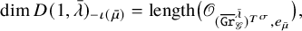 $$\begin{align*}\dim D(1,\bar{\lambda})_{- \iota(\bar{\mu}) }= \mathrm{length} \big ( \mathscr{O}_{ (\overline{\operatorname{\mathrm{\mathtt{Gr}}}}_{{\mathscr{G}} }^{\bar{\lambda}})^{T^\sigma} , e_{\bar{\mu}} } \big ), \end{align*}$$
where $D(1,\bar {\lambda })_{-\iota (\bar {\mu } ) } $
is the
$D(1,\bar {\lambda })_{-\iota (\bar {\mu } ) } $
is the $-\iota (\bar {\mu })$
-weight space in
$-\iota (\bar {\mu })$
-weight space in $D(1,\bar {\lambda })$
. We will prove that for any
$D(1,\bar {\lambda })$
. We will prove that for any $\bar {\mu }\precneqq \bar {\lambda }$
,
$\bar {\mu }\precneqq \bar {\lambda }$
, $\dim D(1,\bar {\lambda })_{- \iota (\bar {\mu }) }\geq 2$
, which would imply that
$\dim D(1,\bar {\lambda })_{- \iota (\bar {\mu }) }\geq 2$
, which would imply that $e_{\bar {\mu }}$
is not a smooth point in
$e_{\bar {\mu }}$
is not a smooth point in $\overline {\operatorname {\mathrm {\mathtt {Gr}}}}_{{\mathscr {G}} }^{\bar {\lambda }}$
. From the surjectivity of (4.6), we have an embedding
$\overline {\operatorname {\mathrm {\mathtt {Gr}}}}_{{\mathscr {G}} }^{\bar {\lambda }}$
. From the surjectivity of (4.6), we have an embedding $D(1, \bar {\mu })\hookrightarrow D(1,\bar {\lambda })$
. However,
$D(1, \bar {\mu })\hookrightarrow D(1,\bar {\lambda })$
. However, $V(-\iota (\bar {\lambda }))\hookrightarrow D(1, \bar {\lambda })$
, where
$V(-\iota (\bar {\lambda }))\hookrightarrow D(1, \bar {\lambda })$
, where $V(-\iota (\bar {\lambda }))$
is the irreducible representation of
$V(-\iota (\bar {\lambda }))$
is the irreducible representation of $\mathfrak {g}^\sigma $
of lowest weight
$\mathfrak {g}^\sigma $
of lowest weight $-\iota (\bar {\lambda })$
. In view of Lemma 2.2, Lemma 3.3 and Lemma 3.4, when G is not of type
$-\iota (\bar {\lambda })$
. In view of Lemma 2.2, Lemma 3.3 and Lemma 3.4, when G is not of type $A_{2\ell }$
, the relation
$A_{2\ell }$
, the relation $\bar {\mu }\precneqq \bar {\lambda }$
implies that
$\bar {\mu }\precneqq \bar {\lambda }$
implies that $\iota (\bar {\mu })\precneqq \iota (\bar {\lambda })$
. Hence,
$\iota (\bar {\mu })\precneqq \iota (\bar {\lambda })$
. Hence, $V(-\iota (\bar {\lambda }))_{ -\iota (\bar {\mu }) }\not =0$
. Furthermore, as subspaces in
$V(-\iota (\bar {\lambda }))_{ -\iota (\bar {\mu }) }\not =0$
. Furthermore, as subspaces in $D(1, \bar {\lambda })$
,
$D(1, \bar {\lambda })$
,
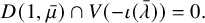 $$\begin{align*}D(1, \bar{\mu})\cap V(-\iota(\bar{\lambda}))=0.\end{align*}$$
It follows that $\dim D(1,\bar {\lambda })_{- \iota (\bar {\mu }) }\geq 2$
. This concludes the proof of the theorem.
$\dim D(1,\bar {\lambda })_{- \iota (\bar {\mu }) }\geq 2$
. This concludes the proof of the theorem.
Now we will deal with the case of $A_{2\ell }^{(2)}$
. Recall the group
$A_{2\ell }^{(2)}$
. Recall the group $H=(\check {G})^\tau $
mentioned in Section 2.3. By the ramified geometric Satake,
$H=(\check {G})^\tau $
mentioned in Section 2.3. By the ramified geometric Satake, $(X_*(T)_\sigma , X_*(T)^+_\sigma , \gamma _j, j\in I_\sigma )$
can be regarded as the weight lattice, the set of dominant weights, and simple roots of H. When
$(X_*(T)_\sigma , X_*(T)^+_\sigma , \gamma _j, j\in I_\sigma )$
can be regarded as the weight lattice, the set of dominant weights, and simple roots of H. When $(G,m)=(A_{2\ell }, 4)$
, H is
$(G,m)=(A_{2\ell }, 4)$
, H is $B_\ell $
of adjoint type. Let
$B_\ell $
of adjoint type. Let $\varpi _1,\varpi _2,\cdots , \varpi _\ell $
be the set of fundamental dominant weights of H.
$\varpi _1,\varpi _2,\cdots , \varpi _\ell $
be the set of fundamental dominant weights of H.
Theorem 4.11. Let ${\mathscr {G}}$
be of type
${\mathscr {G}}$
be of type $A_{2\ell }^{(2)}$
. For any
$A_{2\ell }^{(2)}$
. For any $\lambda \in X_*(T)_\sigma ^+$
, the smooth locus of
$\lambda \in X_*(T)_\sigma ^+$
, the smooth locus of $\overline {\operatorname {\mathrm {\mathtt {Gr}}}}_{{\mathscr {G}} }^{\bar {\lambda }}$
is exactly the union of
$\overline {\operatorname {\mathrm {\mathtt {Gr}}}}_{{\mathscr {G}} }^{\bar {\lambda }}$
is exactly the union of $\operatorname {\mathrm {\mathtt {Gr}}}_{{\mathscr {G}} }^{\bar {\lambda }}$
and those
$\operatorname {\mathrm {\mathtt {Gr}}}_{{\mathscr {G}} }^{\bar {\lambda }}$
and those $\operatorname {\mathrm {\mathtt {Gr}}}_{{\mathscr {G}} }^{\bar {\mu }}$
such that
$\operatorname {\mathrm {\mathtt {Gr}}}_{{\mathscr {G}} }^{\bar {\mu }}$
such that $ \bar {\lambda }-\bar {\mu }=\sum _{j=i}^\ell \gamma _j$
and
$ \bar {\lambda }-\bar {\mu }=\sum _{j=i}^\ell \gamma _j$
and $\mu =\sum _{k=1}^{i-1 } a_k\varpi _k$
with all
$\mu =\sum _{k=1}^{i-1 } a_k\varpi _k$
with all $a_k\in \mathbb {Z}^{\geq 0}$
, for some
$a_k\in \mathbb {Z}^{\geq 0}$
, for some $1\leq i\leq \ell $
.
$1\leq i\leq \ell $
.
Proof. We first prove the following result: for any $\bar {\lambda }, \bar {\mu }\in X_*(T)_\sigma ^+$
with
$\bar {\lambda }, \bar {\mu }\in X_*(T)_\sigma ^+$
with $\bar {\mu }\precneqq \bar {\lambda }$
, the Schubert cell
$\bar {\mu }\precneqq \bar {\lambda }$
, the Schubert cell $\operatorname {\mathrm {\mathtt {Gr}}}_{\mathscr {G}}^{\bar {\mu }}$
is contained in the singular locus of
$\operatorname {\mathrm {\mathtt {Gr}}}_{\mathscr {G}}^{\bar {\mu }}$
is contained in the singular locus of $\overline {\operatorname {\mathrm {\mathtt {Gr}}}}_{\mathscr {G}}^{\bar {\lambda }} $
, except when
$\overline {\operatorname {\mathrm {\mathtt {Gr}}}}_{\mathscr {G}}^{\bar {\lambda }} $
, except when $\bar {\mu } \prec \bar {\lambda } $
is a cover relation and the simple short root
$\bar {\mu } \prec \bar {\lambda } $
is a cover relation and the simple short root $\gamma _\ell $
appears in
$\gamma _\ell $
appears in $\bar {\lambda }-\bar {\mu }$
. We will prove this fact by several steps. Let
$\bar {\lambda }-\bar {\mu }$
. We will prove this fact by several steps. Let $c_\ell $
be the coefficient of
$c_\ell $
be the coefficient of $\gamma _\ell $
in
$\gamma _\ell $
in $\bar {\lambda }-\bar {\mu }$
.
$\bar {\lambda }-\bar {\mu }$
.
Step 1. Observe that using Lemma 3.3 and by the same proof of Theorem 4.10, when the coefficient $c_\ell $
is even, we have
$c_\ell $
is even, we have $\dim D(1,\bar {\lambda })_{-\iota (\bar {\mu } )}\geq 2$
. Thus,
$\dim D(1,\bar {\lambda })_{-\iota (\bar {\mu } )}\geq 2$
. Thus, $e_{\bar {\mu }}$
is singular in
$e_{\bar {\mu }}$
is singular in $\overline {\operatorname {\mathrm {\mathtt {Gr}}}}_{\mathscr {G}}^{\bar {\lambda }} $
.
$\overline {\operatorname {\mathrm {\mathtt {Gr}}}}_{\mathscr {G}}^{\bar {\lambda }} $
.
Step 2. Assume that the coefficient $c_\ell>1$
and
$c_\ell>1$
and $c_\ell $
is odd. There exists sequence of dominant elements in
$c_\ell $
is odd. There exists sequence of dominant elements in $X_*(T)^+_\sigma $
,
$X_*(T)^+_\sigma $
,
 $$ \begin{align} \bar{\mu}= \bar{\lambda}_k \prec \bar{\lambda}_{k-1} \prec \cdots \prec \bar{\lambda}_1 \prec \bar{\lambda}_{0} = \bar{\lambda} , \end{align} $$
such that each $\prec $
is a cover relation. Then, by a theorem of Stembridge [Reference StembridgeSt, Theorem 2.8], for each i,
$\prec $
is a cover relation. Then, by a theorem of Stembridge [Reference StembridgeSt, Theorem 2.8], for each i, $ \bar {\lambda }_{i} - \bar {\lambda }_{i+1} $
is a positive root of H, for any
$ \bar {\lambda }_{i} - \bar {\lambda }_{i+1} $
is a positive root of H, for any $0\leq i \leq k-1$
, and the coefficient of
$0\leq i \leq k-1$
, and the coefficient of $\gamma _\ell $
in each
$\gamma _\ell $
in each $ \bar {\lambda }_{i} - \bar {\lambda }_{i+1}$
is either 0 or 1. Let j be the least integer such that the coefficient of
$ \bar {\lambda }_{i} - \bar {\lambda }_{i+1}$
is either 0 or 1. Let j be the least integer such that the coefficient of $\gamma _\ell $
in
$\gamma _\ell $
in $\bar {\lambda }_{j-1}-\bar {\lambda }_j$
is 1. Such j exists, since
$\bar {\lambda }_{j-1}-\bar {\lambda }_j$
is 1. Such j exists, since $c_\ell \not =1$
. Then the coefficient of
$c_\ell \not =1$
. Then the coefficient of $\gamma _\ell $
in
$\gamma _\ell $
in $\bar {\lambda }_j- \bar {\mu }$
is even. By Step 1, we have
$\bar {\lambda }_j- \bar {\mu }$
is even. By Step 1, we have $\dim D(1,\bar {\lambda }_j )_{-\iota (\bar {\mu } )}\geq 2$
. However, we have the inclusion
$\dim D(1,\bar {\lambda }_j )_{-\iota (\bar {\mu } )}\geq 2$
. However, we have the inclusion $D(1,\bar {\lambda }_j )\subset D(1,\bar {\lambda })$
. It follows that
$D(1,\bar {\lambda }_j )\subset D(1,\bar {\lambda })$
. It follows that $\dim D(1,\bar {\lambda })_{-\iota (\bar {\mu } )}\geq 2$
. Hence, the variety
$\dim D(1,\bar {\lambda })_{-\iota (\bar {\mu } )}\geq 2$
. Hence, the variety $\overline {\operatorname {\mathrm {\mathtt {Gr}}}}^{\bar {\lambda }}_{\mathscr {G}}$
is singular at the point
$\overline {\operatorname {\mathrm {\mathtt {Gr}}}}^{\bar {\lambda }}_{\mathscr {G}}$
is singular at the point $e_{\bar {\mu }}$
.
$e_{\bar {\mu }}$
.
Step 3. We now assume that the coefficient $c_\ell =1$
. By assumption,
$c_\ell =1$
. By assumption, $\bar {\mu }\prec \bar {\lambda }$
is not a cover relation. Then, in the sequence of cover relations in (4.13), either the coefficient of
$\bar {\mu }\prec \bar {\lambda }$
is not a cover relation. Then, in the sequence of cover relations in (4.13), either the coefficient of $\gamma _\ell $
in
$\gamma _\ell $
in $ \bar {\lambda }_{k-1} - \bar {\lambda }_{k} $
is 0 or the coefficient of
$ \bar {\lambda }_{k-1} - \bar {\lambda }_{k} $
is 0 or the coefficient of $\gamma _\ell $
in
$\gamma _\ell $
in $ \bar {\lambda }_{0} - \bar {\lambda }_{1} $
is 0. If the coefficient of
$ \bar {\lambda }_{0} - \bar {\lambda }_{1} $
is 0. If the coefficient of $\gamma _\ell $
in
$\gamma _\ell $
in $ \bar {\lambda }_{k-1} - \bar {\lambda }_{k} $
is 0, by Step 1,
$ \bar {\lambda }_{k-1} - \bar {\lambda }_{k} $
is 0, by Step 1, $\dim D(1,\bar {\lambda }_{k-1} )_{-\iota (\bar {\mu })}\geq 2$
, implying that
$\dim D(1,\bar {\lambda }_{k-1} )_{-\iota (\bar {\mu })}\geq 2$
, implying that $\dim D(1,\bar {\lambda })_{-\iota (\bar {\mu })}\geq 2$
. Hence,
$\dim D(1,\bar {\lambda })_{-\iota (\bar {\mu })}\geq 2$
. Hence, $e_{\bar {\mu }}$
is singular in
$e_{\bar {\mu }}$
is singular in $\overline {\operatorname {\mathrm {\mathtt {Gr}}}}_{\mathscr {G}}^{\bar {\lambda }}$
. If the coefficient of
$\overline {\operatorname {\mathrm {\mathtt {Gr}}}}_{\mathscr {G}}^{\bar {\lambda }}$
. If the coefficient of $\gamma _\ell $
in
$\gamma _\ell $
in $ \bar {\lambda }_{0} - \bar {\lambda }_{1} $
is 0, then by Step 1 again,
$ \bar {\lambda }_{0} - \bar {\lambda }_{1} $
is 0, then by Step 1 again, $e_{\bar {\lambda }_1}$
is a singular point in
$e_{\bar {\lambda }_1}$
is a singular point in $\overline {\operatorname {\mathrm {\mathtt {Gr}}}}_{\mathscr {G}}^{\bar {\lambda }}$
. Since the singular locus of
$\overline {\operatorname {\mathrm {\mathtt {Gr}}}}_{\mathscr {G}}^{\bar {\lambda }}$
. Since the singular locus of $\overline {\operatorname {\mathrm {\mathtt {Gr}}}}_{\mathscr {G}}^{\bar {\lambda }}$
is closed, the point
$\overline {\operatorname {\mathrm {\mathtt {Gr}}}}_{\mathscr {G}}^{\bar {\lambda }}$
is closed, the point $e_{\bar {\mu }}$
is also singular in
$e_{\bar {\mu }}$
is also singular in $\overline {\operatorname {\mathrm {\mathtt {Gr}}}}_{\mathscr {G}}^{\bar {\lambda }}$
.
$\overline {\operatorname {\mathrm {\mathtt {Gr}}}}_{\mathscr {G}}^{\bar {\lambda }}$
.
We now explicitly describe the cover relation $\bar {\mu }\prec \bar {\lambda }$
such that
$\bar {\mu }\prec \bar {\lambda }$
such that $\gamma _\ell $
appears in
$\gamma _\ell $
appears in $\bar {\lambda }-\bar {\mu }$
. Note that
$\bar {\lambda }-\bar {\mu }$
. Note that $X_*(T)_\sigma $
is a root lattice of
$X_*(T)_\sigma $
is a root lattice of $H\simeq \mathrm {SO}_{2n+1}$
. In fact, the lattice
$H\simeq \mathrm {SO}_{2n+1}$
. In fact, the lattice $X_*(T)_\sigma $
is spanned by
$X_*(T)_\sigma $
is spanned by $\varpi _1,\varpi _2, \cdots , \varpi _{\ell -1}, 2\varpi _\ell $
. Reading more carefully from [Reference StembridgeSt, Theorem 2.8], we can see that
$\varpi _1,\varpi _2, \cdots , \varpi _{\ell -1}, 2\varpi _\ell $
. Reading more carefully from [Reference StembridgeSt, Theorem 2.8], we can see that $\bar {\mu }\prec \bar {\lambda }$
is a cover relation and
$\bar {\mu }\prec \bar {\lambda }$
is a cover relation and $\gamma _\ell $
appears in
$\gamma _\ell $
appears in $ \bar {\lambda }-\bar {\mu }$
, if and only if one of the followings holds:
$ \bar {\lambda }-\bar {\mu }$
, if and only if one of the followings holds:
-
1.
$ \bar {\lambda }-\bar {\mu }=\gamma _\ell $
and
$\langle \bar {\mu }, \check {\gamma }_\ell \rangle \neq 0 $
, where
$\check {\gamma }_\ell $
is the coroot of
$\gamma _\ell $
. -
2.
$ \bar {\lambda }-\bar {\mu }=\sum _{j=i}^\ell \gamma _j$
and
$\mu =\sum _{k=1}^{i-1 } a_k\varpi _k$
, for some
$1\leq i\leq \ell $
.


Let G be the simply-connected simple group of type $A_{2\ell }$
with the standard automorphism
$A_{2\ell }$
with the standard automorphism $\sigma $
considered in this paper. Let
$\sigma $
considered in this paper. Let $\alpha _1,\alpha _2,\cdots , \alpha _{2\ell }$
is a set of simple roots of G. Let L be the Levi subgroup of G generated by the simple roots
$\alpha _1,\alpha _2,\cdots , \alpha _{2\ell }$
is a set of simple roots of G. Let L be the Levi subgroup of G generated by the simple roots
 $$\begin{align*}\alpha_{i}, \alpha_{i+1},\cdots, \alpha_{\ell}, \alpha_{\ell+1}, \cdots, \alpha_{\ell+i} , \alpha_{\ell+i+1}.\end{align*}$$
Let M be the derived group $[L,L]$
of L. Then M is simply-connected simple group of type
$[L,L]$
of L. Then M is simply-connected simple group of type $A_{ 2(\ell -i+1)}$
and
$A_{ 2(\ell -i+1)}$
and $\sigma $
still acts on M as a standard automorphism. Let
$\sigma $
still acts on M as a standard automorphism. Let $\mathscr {M}$
be the parahoric group scheme
$\mathscr {M}$
be the parahoric group scheme $\mathrm {Res}_{\mathcal {O}/\bar {\mathcal {O} } } (M_{\mathcal {O}})^\sigma $
, which is of type
$\mathrm {Res}_{\mathcal {O}/\bar {\mathcal {O} } } (M_{\mathcal {O}})^\sigma $
, which is of type $A_{2(\ell -i+1)}^{(2)}$
. Let
$A_{2(\ell -i+1)}^{(2)}$
. Let $T'=T\cap M$
be the maximal torus of M. We have the inclusion
$T'=T\cap M$
be the maximal torus of M. We have the inclusion $X_*(T')\to X_*(T)$
, and this induces an inclusion
$X_*(T')\to X_*(T)$
, and this induces an inclusion $X_*(T')_\sigma \to X_*(T)_\sigma $
and
$X_*(T')_\sigma \to X_*(T)_\sigma $
and $X_*(T')^+_\sigma \to X_*(T)^+_\sigma $
. We write
$X_*(T')^+_\sigma \to X_*(T)^+_\sigma $
. We write $\bar {\lambda }=\sum _{k=1}^\ell b_k \varpi _k$
and
$\bar {\lambda }=\sum _{k=1}^\ell b_k \varpi _k$
and $\bar {\mu }=\sum _{k=1}^\ell c_k \varpi _k$
with
$\bar {\mu }=\sum _{k=1}^\ell c_k \varpi _k$
with $b_k\geq 0, c_k\geq 0$
for any
$b_k\geq 0, c_k\geq 0$
for any $k=1,\cdots , \ell $
. Set
$k=1,\cdots , \ell $
. Set
 $$\begin{align*}\bar{\lambda}' =\sum_{k=i}^{\ell} b_k \varpi_k, \quad \bar{\mu}' =\sum_{k=i}^{\ell} c_k \varpi_k .\end{align*}$$
Then, $\bar {\lambda }', \bar {\mu }' \in X_*(T')^+_\sigma $
. Moreover,
$\bar {\lambda }', \bar {\mu }' \in X_*(T')^+_\sigma $
. Moreover, $\bar {\lambda }'- \bar {\mu }' =\bar {\lambda }-\bar {\mu }$
. We have the following twisted analogue of Levi lemma,
$\bar {\lambda }'- \bar {\mu }' =\bar {\lambda }-\bar {\mu }$
. We have the following twisted analogue of Levi lemma,
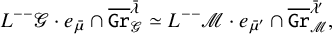 $$ \begin{align} L^{--}{\mathscr{G}}\cdot e_{\bar{\mu}} \cap \overline{\operatorname{\mathrm{\mathtt{Gr}}}}^{\bar{\lambda}}_{\mathscr{G}} \simeq L^{--}\mathscr{M}\cdot e_{\bar{\mu}' } \cap \overline{\operatorname{\mathrm{\mathtt{Gr}}}}^{\bar{\lambda}' }_{\mathscr{M}} , \end{align} $$
where $ L^{--}{\mathscr {G}}$
and
$ L^{--}{\mathscr {G}}$
and $L^{--}\mathscr {M}$
are defined as in (4.1). It can be proved by exactly the same argument as in [Reference Malkin, Ostrik and VybornovMOV, Corollary 3.4], relying on the following main ingredients:
$L^{--}\mathscr {M}$
are defined as in (4.1). It can be proved by exactly the same argument as in [Reference Malkin, Ostrik and VybornovMOV, Corollary 3.4], relying on the following main ingredients:
-
1.
$L^{--}{\mathscr {G}}\cdot e_{\bar {0}}$
(resp.
$L^{--}\mathscr {M}\cdot e_{\bar {0}}$
) is open in
$\operatorname {\mathrm {\mathtt {Gr}}}_{\mathscr {G}}$
(resp.
$\operatorname {\mathrm {\mathtt {Gr}}}_{\mathscr {M}}$
); cf. (4.2). -
2. Transversal slice lemma for
$\operatorname {\mathrm {\mathtt {Gr}}}_{\mathscr {G}}$
and
$\operatorname {\mathrm {\mathtt {Gr}}}_{\mathscr {M}}$
(cf. [Reference Malkin, Ostrik and VybornovMOV, Lemma 2.5], [Reference Kazhdan and LusztigKLu, Section 1.4]); that is,
$ L^{--}{\mathscr {G}}\cdot e_{\bar {\mu }}$
(resp.
$ L^{--}\mathscr {M}\cdot e_{\bar {\mu }' }$
) is a transverse slice to
$\overline {\operatorname {\mathrm {\mathtt {Gr}}}}^{\bar {\lambda }}_{\mathscr {G}}$
(resp.
$ \overline {\operatorname {\mathrm {\mathtt {Gr}}}}^{\bar {\lambda }' }_{\mathscr {M}}$
). -
3.
$L^{--}{\mathscr {G}}\cdot e_{\bar {\mu }} \cap \overline {\operatorname {\mathrm {\mathtt {Gr}}}}^{\bar {\lambda }}_{\mathscr {G}}$
and
$L^{--}\mathscr {M}\cdot e_{\bar {\mu }' } \cap \overline {\operatorname {\mathrm {\mathtt {Gr}}}}^{\bar {\lambda }' }_{\mathscr {M}} $
are reduced, irreducible and normal; cf. [Reference Malkin, Ostrik and VybornovMOV, Lemma 2.6]. Here, the main point is that
$ \overline {\operatorname {\mathrm {\mathtt {Gr}}}}^{\bar {\lambda }}_{\mathscr {G}}$
and
$ \overline {\operatorname {\mathrm {\mathtt {Gr}}}}^{\bar {\lambda }' }_{\mathscr {M}}$
are normal, cf. [Reference Pappas and RapoportPR, Theorem 0.3].


From the isomorphism (4.14) and the transversal slice lemma, we have the following Levi reduction: $e_{\bar {\mu }' }$
is singular in
$e_{\bar {\mu }' }$
is singular in $\overline {\operatorname {\mathrm {\mathtt {Gr}}}}_{\mathscr {M}}^{\bar {\lambda }' }$
if and only if
$\overline {\operatorname {\mathrm {\mathtt {Gr}}}}_{\mathscr {M}}^{\bar {\lambda }' }$
if and only if $e_{\bar {\mu }}$
is singular in
$e_{\bar {\mu }}$
is singular in $\overline {\operatorname {\mathrm {\mathtt {Gr}}}}^{\bar {\lambda }}_{\mathscr {G}} $
.
$\overline {\operatorname {\mathrm {\mathtt {Gr}}}}^{\bar {\lambda }}_{\mathscr {G}} $
.
Case (1): $ \bar {\lambda }-\bar {\mu }=\gamma _\ell $
and
$ \bar {\lambda }-\bar {\mu }=\gamma _\ell $
and $\langle \bar {\mu }, \check {\gamma }_\ell \rangle \neq 0 $
. In this case, we are reduced to
$\langle \bar {\mu }, \check {\gamma }_\ell \rangle \neq 0 $
. In this case, we are reduced to $A_2^{(2)}$
. It is known from [Reference Haines and RicharzHR, Proposition 7.1] that
$A_2^{(2)}$
. It is known from [Reference Haines and RicharzHR, Proposition 7.1] that $e_{\bar {\mu }' }$
is singular in
$e_{\bar {\mu }' }$
is singular in $\overline {\operatorname {\mathrm {\mathtt {Gr}}}}_{\mathscr {M}}^{\bar {\lambda }' }$
, as
$\overline {\operatorname {\mathrm {\mathtt {Gr}}}}_{\mathscr {M}}^{\bar {\lambda }' }$
, as $\bar {\lambda }'$
is not quasi-minuscule.
$\bar {\lambda }'$
is not quasi-minuscule.
Case (2): $ \bar {\lambda }-\bar {\mu }=\sum _{j=i}^\ell \gamma _j$
and
$ \bar {\lambda }-\bar {\mu }=\sum _{j=i}^\ell \gamma _j$
and $\mu =\sum _{k=1}^{i-1 } a_k\varpi _k$
with all
$\mu =\sum _{k=1}^{i-1 } a_k\varpi _k$
with all $a_k>0$
, for some
$a_k>0$
, for some $1\leq i\leq \ell $
. In this case,
$1\leq i\leq \ell $
. In this case, $\bar {\mu }'=0$
and
$\bar {\mu }'=0$
and $\bar {\lambda }'=\sum _{j=i}^\ell \gamma _j$
. Thus, we are reduced to consider the singularity of quasi-minuscule affine Schubert variety
$\bar {\lambda }'=\sum _{j=i}^\ell \gamma _j$
. Thus, we are reduced to consider the singularity of quasi-minuscule affine Schubert variety $\overline {\operatorname {\mathrm {\mathtt {Gr}}}}_{\mathscr {M}}^{\bar {\lambda }' }$
. It was observed by Richarz (using [Reference ArzdorfArz, Prop 4.16]) that the variety
$\overline {\operatorname {\mathrm {\mathtt {Gr}}}}_{\mathscr {M}}^{\bar {\lambda }' }$
. It was observed by Richarz (using [Reference ArzdorfArz, Prop 4.16]) that the variety $\overline {\operatorname {\mathrm {\mathtt {Gr}}}}_{\mathscr {M}}^{\bar {\lambda }' }$
is smooth. We give a different argument here. We consider the parahoric group scheme
$\overline {\operatorname {\mathrm {\mathtt {Gr}}}}_{\mathscr {M}}^{\bar {\lambda }' }$
is smooth. We give a different argument here. We consider the parahoric group scheme ${\mathscr {G}}=\mathrm { Res}_{\mathcal {O}/\bar {\mathcal {O} } } (G_{\mathcal {O}})^\sigma $
, and let
${\mathscr {G}}=\mathrm { Res}_{\mathcal {O}/\bar {\mathcal {O} } } (G_{\mathcal {O}})^\sigma $
, and let $\overline {\operatorname {\mathrm {\mathtt {Gr}}}}_{\mathscr {G}}^ {\bar {\lambda }}$
be the quasi-minuscule Schubert variety. Let
$\overline {\operatorname {\mathrm {\mathtt {Gr}}}}_{\mathscr {G}}^ {\bar {\lambda }}$
be the quasi-minuscule Schubert variety. Let $\mathfrak {g}_{\mathrm {i}}$
be the eigenspace of
$\mathfrak {g}_{\mathrm {i}}$
be the eigenspace of $\sigma $
on the Lie algebra
$\sigma $
on the Lie algebra $\mathfrak {g}$
of eigenvalue
$\mathfrak {g}$
of eigenvalue $\mathrm {i}=\sqrt {-1}$
. The vector space
$\mathrm {i}=\sqrt {-1}$
. The vector space $\mathfrak {g}_{\mathrm {i}}$
consists of two
$\mathfrak {g}_{\mathrm {i}}$
consists of two $G^\sigma $
-orbits, as
$G^\sigma $
-orbits, as $\mathfrak {g}_{\mathrm {i}}$
is actually the standard representation of
$\mathfrak {g}_{\mathrm {i}}$
is actually the standard representation of $G^\sigma =\mathrm {Sp}_{2\ell }$
which is of dimension
$G^\sigma =\mathrm {Sp}_{2\ell }$
which is of dimension $2\ell $
. Thus, any element in
$2\ell $
. Thus, any element in $\mathfrak {g}_{\mathrm {i}}$
is nilpotent. Then we consider a
$\mathfrak {g}_{\mathrm {i}}$
is nilpotent. Then we consider a $G^\sigma $
-equivariant embedding
$G^\sigma $
-equivariant embedding $\mathfrak {g}_{\mathrm {i}}\to {\operatorname {\mathrm {\mathtt {Gr}}}}_{\mathscr {G}}$
given by
$\mathfrak {g}_{\mathrm {i}}\to {\operatorname {\mathrm {\mathtt {Gr}}}}_{\mathscr {G}}$
given by $x\mapsto \mathrm { exp}(( \mathrm {ad } x)t^{-1}) \cdot e_{0}\in {\operatorname {\mathrm {\mathtt {Gr}}}}_{\mathscr {G}}$
, where
$x\mapsto \mathrm { exp}(( \mathrm {ad } x)t^{-1}) \cdot e_{0}\in {\operatorname {\mathrm {\mathtt {Gr}}}}_{\mathscr {G}}$
, where $e_0$
is the base point in
$e_0$
is the base point in $\operatorname {\mathrm {\mathtt {Gr}}}_{\mathscr {G}}$
, and we regard
$\operatorname {\mathrm {\mathtt {Gr}}}_{\mathscr {G}}$
, and we regard $\mathrm {ad} x$
as an element in
$\mathrm {ad} x$
as an element in $G=G_{ad}$
. Since
$G=G_{ad}$
. Since $e_\ell + e_{\ell +1}\in \mathfrak {g}_{\mathrm {i}}$
, and
$e_\ell + e_{\ell +1}\in \mathfrak {g}_{\mathrm {i}}$
, and $\{ e_\ell + e_{\ell +1}, f_\ell +f_{\ell +1}, h_{\ell }+h_{\ell +1} \}$
form a
$\{ e_\ell + e_{\ell +1}, f_\ell +f_{\ell +1}, h_{\ell }+h_{\ell +1} \}$
form a $sl_2$
-triple, one may check easily that
$sl_2$
-triple, one may check easily that $\mathfrak {g}_{\mathrm {i}}$
is mapped into
$\mathfrak {g}_{\mathrm {i}}$
is mapped into $\overline {\operatorname {\mathrm {\mathtt {Gr}}}}_{\mathscr {G}}^{\gamma _\ell }=\overline {\operatorname {\mathrm {\mathtt {Gr}}}}_{\mathscr {G}}^{\bar {\lambda }}$
– in particular,
$\overline {\operatorname {\mathrm {\mathtt {Gr}}}}_{\mathscr {G}}^{\gamma _\ell }=\overline {\operatorname {\mathrm {\mathtt {Gr}}}}_{\mathscr {G}}^{\bar {\lambda }}$
– in particular, $0\mapsto e_0$
. By comparing their dimensions and
$0\mapsto e_0$
. By comparing their dimensions and $G^\sigma $
-equivariance, one may see this is an open embedding. Thus,
$G^\sigma $
-equivariance, one may see this is an open embedding. Thus, $\overline {\operatorname {\mathrm {\mathtt {Gr}}}}_{\mathscr {G}}^{\bar {\lambda }}$
is smooth.
$\overline {\operatorname {\mathrm {\mathtt {Gr}}}}_{\mathscr {G}}^{\bar {\lambda }}$
is smooth.
Remark 4.12. When ${\mathscr {G}}$
is absolutely special of type
${\mathscr {G}}$
is absolutely special of type $A_{2\ell }^{(2)}$
, the smooth locus of twisted affine Schubert variety
$A_{2\ell }^{(2)}$
, the smooth locus of twisted affine Schubert variety $\overline {\operatorname {\mathrm {\mathtt {Gr}}}}_{{\mathscr {G}} }^{\bar {\lambda }} $
is the big cell. This was proved by Richarz in [Reference RicharzRi2]. The idea is to use Levi reduction lemma of Malkin-Ostrik-Vybornov and Stembridge’s combinatorial result [Reference StembridgeSt, Theorem 2.8] to reduce to split rank one cases – in particular, the case
$\overline {\operatorname {\mathrm {\mathtt {Gr}}}}_{{\mathscr {G}} }^{\bar {\lambda }} $
is the big cell. This was proved by Richarz in [Reference RicharzRi2]. The idea is to use Levi reduction lemma of Malkin-Ostrik-Vybornov and Stembridge’s combinatorial result [Reference StembridgeSt, Theorem 2.8] to reduce to split rank one cases – in particular, the case $A_{2}^{(2)}$
(a proof of this case also appears in [Reference Haines and RicharzHR, Prop.7.1]), and the quasi-minuscule Schubert variety (a strong result of this case was proved by Zhu [Reference ZhuZh2] that this variety is not Gorenstein). For the remaining cases, one can use nontriviality of Kazhdan-Lusztig polynomials; cf. [Reference Malkin, Ostrik and VybornovMOV, Prop.6.4.3].
$A_{2}^{(2)}$
(a proof of this case also appears in [Reference Haines and RicharzHR, Prop.7.1]), and the quasi-minuscule Schubert variety (a strong result of this case was proved by Zhu [Reference ZhuZh2] that this variety is not Gorenstein). For the remaining cases, one can use nontriviality of Kazhdan-Lusztig polynomials; cf. [Reference Malkin, Ostrik and VybornovMOV, Prop.6.4.3].
Remark 4.13. One can define the affine Grassmannian $\operatorname {\mathrm {\mathtt {Gr}}}_{{\mathscr {G}} }$
and twisted affine Schubert varieties
$\operatorname {\mathrm {\mathtt {Gr}}}_{{\mathscr {G}} }$
and twisted affine Schubert varieties $\overline {\operatorname {\mathrm {\mathtt {Gr}}}}_{{\mathscr {G}} }^{\bar {\lambda }} $
of the special parahoric group scheme
$\overline {\operatorname {\mathrm {\mathtt {Gr}}}}_{{\mathscr {G}} }^{\bar {\lambda }} $
of the special parahoric group scheme ${\mathscr {G}}$
with the base field
${\mathscr {G}}$
with the base field $\mathrm {k}$
of characteristic p. In [Reference Haines and RicharzHR, Section 6], when
$\mathrm {k}$
of characteristic p. In [Reference Haines and RicharzHR, Section 6], when $p\not = r$
, Haines and Richarz reduced the question of the smooth locus of the
$p\not = r$
, Haines and Richarz reduced the question of the smooth locus of the $\overline {\operatorname {\mathrm {\mathtt {Gr}}}}_{{\mathscr {G}} }^{\bar {\lambda }} $
over characteristic p to characteristic zero case. In fact, by the work of Lourenço [Reference LourençoLo], one may construct a global twisted affine Schubert variety over
$\overline {\operatorname {\mathrm {\mathtt {Gr}}}}_{{\mathscr {G}} }^{\bar {\lambda }} $
over characteristic p to characteristic zero case. In fact, by the work of Lourenço [Reference LourençoLo], one may construct a global twisted affine Schubert variety over $\mathbb {Z}$
so that the base change to the field
$\mathbb {Z}$
so that the base change to the field $\mathrm {k}$
of characteristic p (including
$\mathrm {k}$
of characteristic p (including $p=r$
) is the given twisted affine Schubert variety defined over
$p=r$
) is the given twisted affine Schubert variety defined over $\mathrm {k}$
.
$\mathrm {k}$
.
5 Duality theorem for
$E_6$

In [Reference ZhuZh1, Proposition 2.1.2], Zhu showed that the duality theorem (cf. Theorem 4.4) holds for any dominant coweight if the theorem holds for all fundamental coweights. For type $E_6$
, Zhu was able to prove that the theorem holds for the fundamental coweights
$E_6$
, Zhu was able to prove that the theorem holds for the fundamental coweights $\check {\omega }_1, \check {\omega }_2, \check {\omega }_3, \check {\omega }_5, \check {\omega }_6$
(Bourbaki labelling). However, the most difficult case
$\check {\omega }_1, \check {\omega }_2, \check {\omega }_3, \check {\omega }_5, \check {\omega }_6$
(Bourbaki labelling). However, the most difficult case $\check {\omega }_4$
remained open. In this section, we will prove that the theorem holds for
$\check {\omega }_4$
remained open. In this section, we will prove that the theorem holds for $\check {\omega }_4$
. Thereby, we complete the duality theorem for
$\check {\omega }_4$
. Thereby, we complete the duality theorem for $E_6$
in general.
$E_6$
in general.
5.1 Some reductions
Let G be a simply-laced simple group of adjoint type. Let T be a maximal torus in G. Let $\mathrm {L}$
be the level one line bundle on
$\mathrm {L}$
be the level one line bundle on $\operatorname {\mathrm {\mathtt {Gr}}}_G$
. For any
$\operatorname {\mathrm {\mathtt {Gr}}}_G$
. For any $\lambda \in X_*(T)$
, a general question is if the following restriction map is an isomorphism:
$\lambda \in X_*(T)$
, a general question is if the following restriction map is an isomorphism:
 $$ \begin{align} H^0(\overline{\operatorname{\mathrm{\mathtt{Gr}}}}_{G}^{\lambda}, \mathrm{L}) \to H^0((\overline{\operatorname{\mathrm{\mathtt{Gr}}}}_G^{\lambda} )^T, \mathrm{L}). \end{align} $$
Zhu proved that this map is always surjective (cf. [Reference ZhuZh1, Prop.2.1.1]), and he also proved that the map is an isomorphism for type $A, D$
and many cases of E.
$A, D$
and many cases of E.
Theorem 5.1. The map (5.1) is an isomorphism for any dominant coweight $\lambda $
when G is of type
$\lambda $
when G is of type $E_6$
.
$E_6$
.
Since Zhu has proved this theorem for $\check {\omega }_1, \check {\omega }_2, \check {\omega }_3, \check {\omega }_5, \check {\omega }_6$
, by [Reference ZhuZh1, Prop.2.1.3], we will only need to prove that the theorem holds for
$\check {\omega }_1, \check {\omega }_2, \check {\omega }_3, \check {\omega }_5, \check {\omega }_6$
, by [Reference ZhuZh1, Prop.2.1.3], we will only need to prove that the theorem holds for $\check {\omega }_4$
.
$\check {\omega }_4$
.
For convenience, we assume that $\lambda $
is dominant and
$\lambda $
is dominant and $\lambda $
is in the coroot lattice, and we set
$\lambda $
is in the coroot lattice, and we set
 $$\begin{align*}D(1,\lambda):= H^0(\overline{\operatorname{\mathrm{\mathtt{Gr}}}}_{G}^{\lambda}, \mathrm{L} ) ^\vee, \quad D^T(1,\lambda):= H^0((\overline{\operatorname{\mathrm{\mathtt{Gr}}}}_G^{\lambda} )^T, \mathrm{L}) ^\vee. \end{align*}$$
Then, we can identify $D^T(1,\lambda )$
as a subspace of the affine Demazure module
$D^T(1,\lambda )$
as a subspace of the affine Demazure module $D(1,\lambda )$
.
$D(1,\lambda )$
.
Let $\tilde {L}(\mathfrak {g})= \mathfrak {g}((t))\oplus \mathbb {C} K\oplus \mathbb {C} d$
be the affine Kac-Moody algebra associated to
$\tilde {L}(\mathfrak {g})= \mathfrak {g}((t))\oplus \mathbb {C} K\oplus \mathbb {C} d$
be the affine Kac-Moody algebra associated to $\mathfrak {g}$
with center K and scaling element d. Let
$\mathfrak {g}$
with center K and scaling element d. Let $\mathscr {H}(\Lambda _0)$
denote the integrable highest weight representation of
$\mathscr {H}(\Lambda _0)$
denote the integrable highest weight representation of $\tilde {L}(\mathfrak {g})$
of highest weight
$\tilde {L}(\mathfrak {g})$
of highest weight $\Lambda _0$
. Let
$\Lambda _0$
. Let $v_0$
be the highest weight vector of
$v_0$
be the highest weight vector of $\mathscr {H}(\Lambda _0)$
. For any
$\mathscr {H}(\Lambda _0)$
. For any $w\in W$
, set
$w\in W$
, set
 $$\begin{align*}v_{w(\lambda)}:= t^{w(\lambda)}\cdot v_0. \end{align*}$$
Then $v_{w(\lambda )}$
is an extremal vector in
$v_{w(\lambda )}$
is an extremal vector in $\mathscr {H}(\Lambda _0)$
, and
$\mathscr {H}(\Lambda _0)$
, and $\mathfrak {h}$
-weight of
$\mathfrak {h}$
-weight of $v_{w(\lambda )}$
is
$v_{w(\lambda )}$
is $-\iota (w(\lambda ))$
, where the map
$-\iota (w(\lambda ))$
, where the map $\iota : X_*(T)\to \mathfrak {h}^\vee $
is induced by the normalized Killing form; cf.(3.2). By the theory of affine Demazure module (cf. [Reference KumarKu, Theorem 8.2.2 (a)]), we have
$\iota : X_*(T)\to \mathfrak {h}^\vee $
is induced by the normalized Killing form; cf.(3.2). By the theory of affine Demazure module (cf. [Reference KumarKu, Theorem 8.2.2 (a)]), we have
 $$\begin{align*}D(1,\lambda) = U(\mathfrak{g}[t] )\cdot v_{w(\lambda)} , \quad \text{ for any }w\in W. \end{align*}$$
Given a Levi subgroup L of G, let M be the derived group $[L,L]$
. Let
$[L,L]$
. Let $\mathfrak {m}$
denote the Lie algebra of M, and denote the current algebra of
$\mathfrak {m}$
denote the Lie algebra of M, and denote the current algebra of $\mathfrak {m}$
by
$\mathfrak {m}$
by $\mathfrak {m}[t]$
. By [Reference ZhuZh1, Corollary 1.3.8, Lemma 2.2.6], we have the following Levi reduction lemma.
$\mathfrak {m}[t]$
. By [Reference ZhuZh1, Corollary 1.3.8, Lemma 2.2.6], we have the following Levi reduction lemma.
Lemma 5.2. If the map (5.1) is an isomorphism for M, then $U(\mathfrak {m}[t] )\cdot v_{w(\lambda )}$
is contained in
$U(\mathfrak {m}[t] )\cdot v_{w(\lambda )}$
is contained in $D^T(1,\lambda )$
, for any element w in the Weyl group W of G.
$D^T(1,\lambda )$
, for any element w in the Weyl group W of G.
Let $\mu $
be a dominant coweight of G such that
$\mu $
be a dominant coweight of G such that $\mu \prec \lambda $
. The following restriction map is surjective:
$\mu \prec \lambda $
. The following restriction map is surjective:
 $$\begin{align*}H^0(\overline{\operatorname{\mathrm{\mathtt{Gr}}}}_{G}^{\lambda}, \mathrm{L} ) \to H^0(\overline{\operatorname{\mathrm{\mathtt{Gr}}}}_{G}^{\mu}, \mathrm{L} ) .\end{align*}$$
Hence, it induces an inclusion $D(1,\mu )\subset D(1,\lambda )$
. The following lemma is easy.
$D(1,\mu )\subset D(1,\lambda )$
. The following lemma is easy.
Lemma 5.3. If the map (5.1) is an isomorphism for $\mu $
, then
$\mu $
, then $D(1,\mu )$
is contained in
$D(1,\mu )$
is contained in $D^T(1, \lambda )$
.
$D^T(1, \lambda )$
.
Let $N_G(T)$
denote the normalizer group of T in G. Then
$N_G(T)$
denote the normalizer group of T in G. Then $N_G(T)$
acts on
$N_G(T)$
acts on $(\overline {\operatorname {\mathrm {\mathtt {Gr}}}}_G^{\lambda } )^T$
and thus on the vector space
$(\overline {\operatorname {\mathrm {\mathtt {Gr}}}}_G^{\lambda } )^T$
and thus on the vector space $D^T(1,\lambda )$
. Note that
$D^T(1,\lambda )$
. Note that
 $$\begin{align*}(\overline{\operatorname{\mathrm{\mathtt{Gr}}}}_G^{\lambda} )^T=(\operatorname{\mathrm{\mathtt{Gr}}}_G)^T\cap \overline{\operatorname{\mathrm{\mathtt{Gr}}}}_G^{\lambda} \simeq \operatorname{\mathrm{\mathtt{Gr}}}_T \cap \overline{\operatorname{\mathrm{\mathtt{Gr}}}}_G^{\lambda} , \end{align*}$$
where the second isomorphism follows from Theorem 4.1. Hence, the Lie algebra $\mathfrak {h}[t]$
acts on
$\mathfrak {h}[t]$
acts on $D^T(1,\lambda )$
.
$D^T(1,\lambda )$
.
Notation 5.4. Let $V(\eta , i)$
denote the irreducible representation of
$V(\eta , i)$
denote the irreducible representation of $\mathfrak {g}$
of highest weight
$\mathfrak {g}$
of highest weight $\eta $
and of degree i with respect to the action of d, that appears in the affine Demazure module
$\eta $
and of degree i with respect to the action of d, that appears in the affine Demazure module $D(1,\lambda )$
. For any
$D(1,\lambda )$
. For any $\mathfrak {h}$
-weight
$\mathfrak {h}$
-weight $\nu $
, we write
$\nu $
, we write $V(\eta , i)_{\nu }$
for the
$V(\eta , i)_{\nu }$
for the $\nu $
-weight space of this representation.
$\nu $
-weight space of this representation.
We now consider the case when G is of type $E_6$
and
$E_6$
and $\lambda =\check {\omega }_4$
. All dominant coweights dominated by
$\lambda =\check {\omega }_4$
. All dominant coweights dominated by $\check {\omega }_4$
are described as follows:
$\check {\omega }_4$
are described as follows:
 $$ \begin{align} 0\prec \check{\omega}_2 \prec \check{\omega}_1+\check{\omega}_6\prec \check{\omega}_4. \end{align} $$
For convenience, we set
 $$\begin{align*}v_{\omega_4}:= v_{w_0(\check{\omega}_4 )}.\end{align*}$$
Then $v_{\omega _4}$
is an extremal weight vector in
$v_{\omega _4}$
is an extremal weight vector in $\mathscr {H}(\Lambda _0)$
whose
$\mathscr {H}(\Lambda _0)$
whose $\mathfrak {h}$
-weight is
$\mathfrak {h}$
-weight is $\omega _4$
, since
$\omega _4$
, since $-w_0(\omega _4)=\omega _4$
and
$-w_0(\omega _4)=\omega _4$
and $\iota (\check {\omega }_4 )=\omega _4$
. The Demazure module
$\iota (\check {\omega }_4 )=\omega _4$
. The Demazure module $D(1, \check {\omega }_4)$
contains
$D(1, \check {\omega }_4)$
contains $V(\omega _4, -3)$
, and
$V(\omega _4, -3)$
, and $v_{\omega _4}$
is the highest weight vector of
$v_{\omega _4}$
is the highest weight vector of $V(\omega _4, -3)$
. By [Reference KleberKl, Section 3], we have the following decomposition:
$V(\omega _4, -3)$
. By [Reference KleberKl, Section 3], we have the following decomposition:
 $$ \begin{align} D(1, \check{\omega}_4)= V(0,0) \oplus V(\omega_2,-1) \oplus V(\omega_1+\omega_6,-2) \oplus V(\omega_2,-2) \oplus V(\omega_4,-3). \end{align} $$
Since Zhu has proved that the map (5.1) is an isomorphism for $\check {\omega }_1$
and
$\check {\omega }_1$
and $\check {\omega }_6$
, hence also for
$\check {\omega }_6$
, hence also for $\check {\omega }_1+\check {\omega }_6$
(cf. [Reference ZhuZh1, Prop.2.1.3]), by Lemma 5.3, we have
$\check {\omega }_1+\check {\omega }_6$
(cf. [Reference ZhuZh1, Prop.2.1.3]), by Lemma 5.3, we have $D(1, \check {\omega }_1+\check {\omega }_6)\subset D^T(1,\check {\omega }_4)$
. Moreover, it is easy to see that
$D(1, \check {\omega }_1+\check {\omega }_6)\subset D^T(1,\check {\omega }_4)$
. Moreover, it is easy to see that
 $$\begin{align*}D(1, \check{\omega}_1+\check{\omega}_6) = V(0,0) \oplus V(\omega_2,-1) \oplus V(\omega_1+\omega_6,-2). \end{align*}$$
It follows that $V(0,0) \oplus V(\omega _2,-1) \oplus V(\omega _1+\omega _6,-2) $
is contained in
$V(0,0) \oplus V(\omega _2,-1) \oplus V(\omega _1+\omega _6,-2) $
is contained in $D^T(1, \check {\omega }_4)$
. Thus, it suffices to show that
$D^T(1, \check {\omega }_4)$
. Thus, it suffices to show that $V(\omega _2,-2)$
and
$V(\omega _2,-2)$
and $V(\omega _4,-3) $
are also contained in
$V(\omega _4,-3) $
are also contained in $D^T(1, \check {\omega }_4)$
. Since
$D^T(1, \check {\omega }_4)$
. Since $D(1, \check {\omega }_4 )$
is
$D(1, \check {\omega }_4 )$
is $N_G(T)$
-stable, it can be further reduced to show that for any dominant weight
$N_G(T)$
-stable, it can be further reduced to show that for any dominant weight $\nu $
of
$\nu $
of $\mathfrak {g}$
, the weight space
$\mathfrak {g}$
, the weight space $V(\omega _2,-2)_\nu $
and
$V(\omega _2,-2)_\nu $
and $V(\omega _4,-3)_\nu $
are contained in
$V(\omega _4,-3)_\nu $
are contained in $D^T(1,\check {\omega }_4 )$
. In the remaining part of this section, we will analyze case by case and show that it is indeed true.
$D^T(1,\check {\omega }_4 )$
. In the remaining part of this section, we will analyze case by case and show that it is indeed true.
5.2 The representation
$V(\omega _4, -3)$

The dominant character of $V(\omega _4)$
is
$V(\omega _4)$
is $e^{\omega _4}+4e^{\omega _1+\omega _6}+15e^{\omega _2}+45e^{0}$
. By Lemma 5.2, we have
$e^{\omega _4}+4e^{\omega _1+\omega _6}+15e^{\omega _2}+45e^{0}$
. By Lemma 5.2, we have $v_{w(\check {\omega }_4 )}\in D^T(1, \check {\omega }_4 )$
for any
$v_{w(\check {\omega }_4 )}\in D^T(1, \check {\omega }_4 )$
for any $w\in W$
. We conclude that
$w\in W$
. We conclude that $V(\omega _4,-3)_{\omega _4}\subset D^T(1,\check {\omega }_4 )$
.
$V(\omega _4,-3)_{\omega _4}\subset D^T(1,\check {\omega }_4 )$
.
5.2.1 The weight space
$V(\omega _4,-3)_{\omega _1+\omega _6}$

In terms of simple roots, we have $\omega _4= 2 \alpha _1 +3\alpha _2+4\alpha _3+6\alpha _4+4\alpha _5+2\alpha _2$
and
$\omega _4= 2 \alpha _1 +3\alpha _2+4\alpha _3+6\alpha _4+4\alpha _5+2\alpha _2$
and $\omega _1+\omega _6= 2 \alpha _1+2 \alpha _2 +3\alpha _3+4\alpha _4+3\alpha _5+2\alpha _6$
. Thus, the difference
$\omega _1+\omega _6= 2 \alpha _1+2 \alpha _2 +3\alpha _3+4\alpha _4+3\alpha _5+2\alpha _6$
. Thus, the difference $\omega _4-(\omega _1+\omega _6)=\alpha _2+\alpha _3+2\alpha _4+\alpha _5$
; in other words, this difference is supported on the Levi of type
$\omega _4-(\omega _1+\omega _6)=\alpha _2+\alpha _3+2\alpha _4+\alpha _5$
; in other words, this difference is supported on the Levi of type $D_4$
with simple roots
$D_4$
with simple roots $\alpha _2, \alpha _3, \alpha _4, \alpha _5$
. By applying Chevalley generators
$\alpha _2, \alpha _3, \alpha _4, \alpha _5$
. By applying Chevalley generators $f_2, f_3,f_4,f_5$
on the highest weight vector
$f_2, f_3,f_4,f_5$
on the highest weight vector $v_{\omega _4}$
, we can get a spanning set of the weight space
$v_{\omega _4}$
, we can get a spanning set of the weight space $V(\omega _4, -3)_{ \omega _1+\omega _6 }$
. By Lemma 5.2, we have
$V(\omega _4, -3)_{ \omega _1+\omega _6 }$
. By Lemma 5.2, we have
 $$\begin{align*}V(\omega_4, -3)_{ \omega_1+\omega_6 }\subset D^T(1, \check{\omega}_4 ). \end{align*}$$
5.2.2 The weight space
$V(\omega _4,-3)_{\omega _2}$

This case requires some brute force. We have the following difference: $\beta =\omega _4-\omega _2=\alpha _1+\alpha _2+2\alpha _3+3\alpha _4+2\alpha _5+\alpha _6$
, whose height is 10.
$\beta =\omega _4-\omega _2=\alpha _1+\alpha _2+2\alpha _3+3\alpha _4+2\alpha _5+\alpha _6$
, whose height is 10.
We actually consider all expressions of the form $f_{{i_1}} \dots f_{{i_{10}}} v_{\omega _4}$
such that this vector is of weight
$f_{{i_1}} \dots f_{{i_{10}}} v_{\omega _4}$
such that this vector is of weight $\omega _2$
; this provides a spanning set of vectors in
$\omega _2$
; this provides a spanning set of vectors in $V(\omega _4,-3)_{\omega _2}$
(with many relations!).
$V(\omega _4,-3)_{\omega _2}$
(with many relations!).
Definition 5.5. We say a nonzero vector of the form $f_{{i_1}} f_{i_2}\dots f_{{i_{10}}} v_{\omega _4}$
is Levi-extremal, if there exists
$f_{{i_1}} f_{i_2}\dots f_{{i_{10}}} v_{\omega _4}$
is Levi-extremal, if there exists $ 1\leq k\leq 10$
, such that
$ 1\leq k\leq 10$
, such that
-
1.
$f_{i_1},f_{i_2},\cdots , f_{i_{k}}$
are contained in a proper Levi subalgebra of
$\mathfrak {g}$
; -
2.
$f_{i_{k+1}}\cdots f_{i_{10}} v_{\omega _4}$
is an extremal vector in
$V(\omega _4,-3)$
.


Observe that any proper Levi subalgebra of $E_6$
is either of type A (or their product) or of type D, and the restriction map (5.1) for these types is always an isomorphism, which is due to Zhu. Then, to show that
$E_6$
is either of type A (or their product) or of type D, and the restriction map (5.1) for these types is always an isomorphism, which is due to Zhu. Then, to show that $V(\omega _4,-3)_{\omega _2}\subset D^T(1,\check {\omega }_4 )$
, by Lemma 5.2, it suffices to prove the following proposition.
$V(\omega _4,-3)_{\omega _2}\subset D^T(1,\check {\omega }_4 )$
, by Lemma 5.2, it suffices to prove the following proposition.
Proposition 5.6. Any nonzero vector $f_{{i_1}} f_{i_2}\dots f_{{i_{10}}} v_{\omega _4}$
of weight
$f_{{i_1}} f_{i_2}\dots f_{{i_{10}}} v_{\omega _4}$
of weight $\omega _2$
is Levi-extremal.
$\omega _2$
is Levi-extremal.
Proof. Before we prove this proposition, we first describe a poset of weights $\mu $
with partial order
$\mu $
with partial order $<$
, such that
$<$
, such that $\mu < \omega _4$
, and
$\mu < \omega _4$
, and $\mu -\omega _2$
is a sum of positive roots. For any two weights
$\mu -\omega _2$
is a sum of positive roots. For any two weights $\mu ,\mu '$
in the poset, we write
$\mu ,\mu '$
in the poset, we write $\mu \xrightarrow {s_i}\mu '$
if
$\mu \xrightarrow {s_i}\mu '$
if $\mu '=s_i(\mu )$
and
$\mu '=s_i(\mu )$
and $\langle \mu , \check {\alpha }_i \rangle \geq 1$
. The partial order
$\langle \mu , \check {\alpha }_i \rangle \geq 1$
. The partial order $<$
of this poset is generated by these simple relations. The weight
$<$
of this poset is generated by these simple relations. The weight $\mu $
will be labelled by
$\mu $
will be labelled by ![]() once the support of
once the support of $\mu -\omega _2$
(as a linear combination of simple roots) is contained in a proper sub-diagram of the Dynkin diagram of
$\mu -\omega _2$
(as a linear combination of simple roots) is contained in a proper sub-diagram of the Dynkin diagram of $E_6$
. We will not describe those weights below the
$E_6$
. We will not describe those weights below the ![]() -labelled weights. In the following two figures, we describe this poset by representing weights respectively in terms of the coordinates with respect to fundamental weights and simple roots. We have the following rules.
-labelled weights. In the following two figures, we describe this poset by representing weights respectively in terms of the coordinates with respect to fundamental weights and simple roots. We have the following rules.
-
1. In the first figure, if
$\mu \xrightarrow {s_i}\mu '$
, then the number at vertex i decreases by 2, and the adjacent vertices increase by 1; -
2. In the second figure, if
$\mu \xrightarrow {s_i}\mu '$
, then the number at vertex i decrease by 1, and no changes elsewhere.


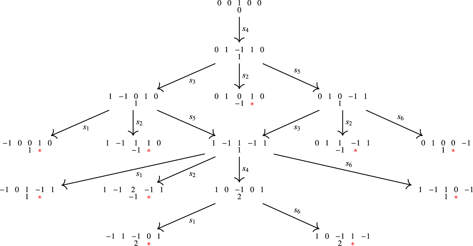
Figure 1 In this diagram, the weight $\mu $
is represented by the coordinates of
$\mu $
is represented by the coordinates of $\mu $
with respect to fundamental weights. When 1 occurs at vertex i, it indicates that we can apply reflection
$\mu $
with respect to fundamental weights. When 1 occurs at vertex i, it indicates that we can apply reflection $s_i$
.
$s_i$
.

Figure 2 This is the same diagram as in Figure 1. The difference is that the weight $\mu $
is represented by the coordinates of
$\mu $
is represented by the coordinates of $\mu -\omega _2$
with respect to simple roots. This diagram tells when the support
$\mu -\omega _2$
with respect to simple roots. This diagram tells when the support $\mu -\omega _2$
is contained in a proper subdiagram.
$\mu -\omega _2$
is contained in a proper subdiagram.
We first show that any nonzero vector $f_{{i_7}}f_{{i_8}}f_{{i_9}}f_{{i_{10}}}v_{\omega _4}$
of weight
$f_{{i_7}}f_{{i_8}}f_{{i_9}}f_{{i_{10}}}v_{\omega _4}$
of weight $\mu $
is an extremal weight vector. This can be easily checked from the first figure, since no integer
$\mu $
is an extremal weight vector. This can be easily checked from the first figure, since no integer $\geq 2$
appears as a coefficient of
$\geq 2$
appears as a coefficient of $\omega _i$
until the 4th step at least. As a result,
$\omega _i$
until the 4th step at least. As a result, $f_{{i_7}}f_{{i_8}}f_{{i_9}}f_{{i_{10}}}v_{\omega _4}=s_{{i_7}}s_{{i_8}}s_{{i_9}}s_{{i_{10}}}v_{\omega _4}$
for any nonzero vector
$f_{{i_7}}f_{{i_8}}f_{{i_9}}f_{{i_{10}}}v_{\omega _4}=s_{{i_7}}s_{{i_8}}s_{{i_9}}s_{{i_{10}}}v_{\omega _4}$
for any nonzero vector $f_{{i_7}}f_{{i_8}}f_{{i_9}}f_{{i_{10}}}v_{\omega _4}$
. Now it is clear from the second figure that any nonzero vector
$f_{{i_7}}f_{{i_8}}f_{{i_9}}f_{{i_{10}}}v_{\omega _4}$
. Now it is clear from the second figure that any nonzero vector $f_{i_1}\cdots f_{{i_7}}f_{{i_8}}f_{{i_9}}f_{{i_{10}}}v_{\omega _4}$
is Levi-extremal if
$f_{i_1}\cdots f_{{i_7}}f_{{i_8}}f_{{i_9}}f_{{i_{10}}}v_{\omega _4}$
is Levi-extremal if
 $$\begin{align*}f_{i_6} f_{{i_7}}f_{{i_8}}f_{{i_9}}f_{i_{10}} \neq f_4f_3f_5f_4=f_4f_5f_3f_4.\end{align*}$$
Thus, the ‘worst possible case’, from the perspective of producing Levi-extremal vectors, has the first four lowering operators as follows: $f_{4}f_{5}f_{3}f_{4} v_{\omega _4}=f_4f_5f_3f_4 v_{\omega _4}$
. All other nontrivial applications of four lowering operators will result in a Levi-extremal vector or the
$f_{4}f_{5}f_{3}f_{4} v_{\omega _4}=f_4f_5f_3f_4 v_{\omega _4}$
. All other nontrivial applications of four lowering operators will result in a Levi-extremal vector or the $0$
vector. We further observe that both
$0$
vector. We further observe that both $f_{1}f_4 f_{5}f_{3}f_{4}v_{\omega _4}$
and
$f_{1}f_4 f_{5}f_{3}f_{4}v_{\omega _4}$
and $f_{6}f_{4}f_{5}f_{3}f_{4}v_{\omega _4}$
result in Levi-extremal vectors.
$f_{6}f_{4}f_{5}f_{3}f_{4}v_{\omega _4}$
result in Levi-extremal vectors.
The only remaining vector to consider is $f_{2}f_{4}f_{5}f_{3}f_{4}v_{\omega _4}$
. Note that this is the first case where
$f_{2}f_{4}f_{5}f_{3}f_{4}v_{\omega _4}$
. Note that this is the first case where $s_{2}s_{4}s_{5}s_{3}s_{4}v_{\omega _4} \neq f_{1}f_{4}f_{5}f_{3}f_{4}v_{\omega _4}$
, since
$s_{2}s_{4}s_{5}s_{3}s_{4}v_{\omega _4} \neq f_{1}f_{4}f_{5}f_{3}f_{4}v_{\omega _4}$
, since $\langle \check {\alpha }_2, \omega _4-2\alpha _4-\alpha _3-\alpha _5 \rangle =2$
. Thus, every element
$\langle \check {\alpha }_2, \omega _4-2\alpha _4-\alpha _3-\alpha _5 \rangle =2$
. Thus, every element $f_{{i_1}} \dots f_{{i_{10}}} v_{\omega _4}$
is Levi-extremal, except those of which the first five lowering operators are precisely
$f_{{i_1}} \dots f_{{i_{10}}} v_{\omega _4}$
is Levi-extremal, except those of which the first five lowering operators are precisely $f_{2}f_{4}f_{5}f_{3}f_{4} $
(up to the order of
$f_{2}f_{4}f_{5}f_{3}f_{4} $
(up to the order of $f_3$
and
$f_3$
and $f_5$
); what remains are the lowering operators
$f_5$
); what remains are the lowering operators $f_1,f_3,f_4,f_5,f_6$
. By the same logic, the next lowering operator must be
$f_1,f_3,f_4,f_5,f_6$
. By the same logic, the next lowering operator must be $f_4$
, since any other lowering operator would commute with
$f_4$
, since any other lowering operator would commute with $f_2$
, returning us to the Levi-extremal vectors situation. Thus, we are left with is considering the element
$f_2$
, returning us to the Levi-extremal vectors situation. Thus, we are left with is considering the element $f_{4}f_{2}f_{4}f_{5}f_{3}f_{4}v_{\omega _4}$
.
$f_{4}f_{2}f_{4}f_{5}f_{3}f_{4}v_{\omega _4}$
.
Note that $f_{\alpha _2+\alpha _4}:=f_{\alpha _4}f_{\alpha _2}-f_{\alpha _2}f_{\alpha _4}$
is a root vector of root
$f_{\alpha _2+\alpha _4}:=f_{\alpha _4}f_{\alpha _2}-f_{\alpha _2}f_{\alpha _4}$
is a root vector of root $\alpha _2+\alpha _4$
. Since
$\alpha _2+\alpha _4$
. Since $f_4f_{4}f_{5}f_{3}f_{4}v_{\omega _4}=0$
, we have
$f_4f_{4}f_{5}f_{3}f_{4}v_{\omega _4}=0$
, we have
 $$\begin{align*}f_{4}f_{2}f_{4}f_{5}f_{3}f_{4}v_{\omega_4}=f_{\alpha_2+\alpha_4}f_{4}f_{5}f_{3}f_{4}v_{\omega_4} .\end{align*}$$
This is the extremal vector $s_{\alpha _2+\alpha _4}s_{4}s_{5}s_{3}s_{4}v_{\omega _4} $
, since the weight of the extremal weight vector
$s_{\alpha _2+\alpha _4}s_{4}s_{5}s_{3}s_{4}v_{\omega _4} $
, since the weight of the extremal weight vector $f_{\alpha _4}f_{\alpha _5}f_{\alpha _3}f_{\alpha _4}v_{\omega _4}$
is
$f_{\alpha _4}f_{\alpha _5}f_{\alpha _3}f_{\alpha _4}v_{\omega _4}$
is $\omega _1+2\omega _2-\omega _4+\omega _6$
, and the pairing
$\omega _1+2\omega _2-\omega _4+\omega _6$
, and the pairing $\langle \omega _1+2 \omega _2-\omega _4+\omega _6,\check {\alpha }_2+\check {\alpha }_4 \rangle =1$
. Our remaining lowering operators are
$\langle \omega _1+2 \omega _2-\omega _4+\omega _6,\check {\alpha }_2+\check {\alpha }_4 \rangle =1$
. Our remaining lowering operators are $f_1,f_3,f_5,f_6$
. They are contained in a proper Levi subalgebra. Thus, any nonzero vector of the form
$f_1,f_3,f_5,f_6$
. They are contained in a proper Levi subalgebra. Thus, any nonzero vector of the form
 $$\begin{align*}f_{i_1}f_{i_2}f_{i_3}f_{i_4} f_{4}f_{2}f_{4}f_{5}f_{3}f_{4}v_{\omega_4} \end{align*}$$
is always Levi-extremal. This concludes the proof.
Remark 5.7. The construction of the above figures comes from the ‘Numbers game’, due to Proctor (unpublished) and explored in Mozes [Reference MozesMo] and Proctor [Reference ProctorPro]. When the representation is minuscule, the action of the simple reflections is described by the algorithm above; adding one to adjacent nodes and subtracting two from the given node (precisely the action of subtracting a simple root in the simply-laced types). While the representation $V(\omega _4)$
is not minuscule or quasi-minuscule, these techniques still proved useful in this case and could be useful for the study of the remaining fundamental representations of
$V(\omega _4)$
is not minuscule or quasi-minuscule, these techniques still proved useful in this case and could be useful for the study of the remaining fundamental representations of $E_7$
and
$E_7$
and $E_8$
, where the restriction isomorphism is not yet known.
$E_8$
, where the restriction isomorphism is not yet known.
5.2.3 The weight space
$V(\omega _4,-3)_0$

Let $\theta $
be the highest root of
$\theta $
be the highest root of $\mathfrak {g}$
, and let
$\mathfrak {g}$
, and let $\beta = \omega _4-\omega _2=\alpha _1+\alpha _2+2\alpha _3+3\alpha _4+2\alpha _5+ \alpha _6$
.
$\beta = \omega _4-\omega _2=\alpha _1+\alpha _2+2\alpha _3+3\alpha _4+2\alpha _5+ \alpha _6$
. $\beta $
is also a positive root of
$\beta $
is also a positive root of $\mathfrak {g}$
. We consider the element
$\mathfrak {g}$
. We consider the element $f_\theta f_{\beta } v_{\omega _4}$
. The following proposition is verified by Travis Scrimshaw using SageMath. See Appendix A.
$f_\theta f_{\beta } v_{\omega _4}$
. The following proposition is verified by Travis Scrimshaw using SageMath. See Appendix A.
Proposition 5.8. The W-span of $f_\theta f_{\beta } v_{\omega _4}$
is the weight zero space
$f_\theta f_{\beta } v_{\omega _4}$
is the weight zero space $V(\omega _4,-3)_0$
.
$V(\omega _4,-3)_0$
.
One can check that $\alpha _1, \alpha _3,\alpha _4,\alpha _5, \theta , -\beta $
form a system of simple positive roots of
$\alpha _1, \alpha _3,\alpha _4,\alpha _5, \theta , -\beta $
form a system of simple positive roots of $E_6$
, and
$E_6$
, and $\theta , -\beta $
form a subsystem of type
$\theta , -\beta $
form a subsystem of type $A_2$
. Then by Lemma 5.2,
$A_2$
. Then by Lemma 5.2, $f_{\theta }f_\beta v_{\omega _4} \in D^T(1,\check {\omega }_4)$
. By W-invariance on
$f_{\theta }f_\beta v_{\omega _4} \in D^T(1,\check {\omega }_4)$
. By W-invariance on $D^T(1,\check {\omega }_4)$
and the above proposition, we can conclude that
$D^T(1,\check {\omega }_4)$
and the above proposition, we can conclude that
 $$ \begin{align} V(\omega_4,-3)_0\subset D^T(1,\check{\omega}_4) .\end{align} $$
5.3 The representation
$V(\omega _2, -2)$

First, we consider the ‘0-string’ of the full basic representation $\mathscr {H}(\Lambda _0)$
; this is the direct sum
$\mathscr {H}(\Lambda _0)$
; this is the direct sum $\oplus _{n\geq 0}\mathscr {H}(\Lambda _0)_{-n\delta }$
. The Weyl group W acts on each of these weight spaces, so
$\oplus _{n\geq 0}\mathscr {H}(\Lambda _0)_{-n\delta }$
. The Weyl group W acts on each of these weight spaces, so $\mathscr {H}(\Lambda _0) _{-n\delta }$
is a direct sum of irreducible representations of the Weyl group W. We first describe
$\mathscr {H}(\Lambda _0) _{-n\delta }$
is a direct sum of irreducible representations of the Weyl group W. We first describe $\mathscr {H}(\Lambda _0)_{-n\delta }$
for
$\mathscr {H}(\Lambda _0)_{-n\delta }$
for $n=0,1,2,3$
, as representations of W. By [Reference KacKa, Proposition 12.13], we have the following decompositions:
$n=0,1,2,3$
, as representations of W. By [Reference KacKa, Proposition 12.13], we have the following decompositions:
 $$\begin{align*}\mathscr{H}(\Lambda_0)_{0}= \mathbb{C} v_0\simeq \mathbb{C} , \end{align*}$$
 $$\begin{align*}\mathscr{H}(\Lambda_0)_{-\delta}= \mathfrak{h} t^{-1}\cdot v_0 \simeq \mathfrak{h} \end{align*}$$
 $$ \begin{align} \mathscr{H}(\Lambda_0)_{-2\delta}= \mathfrak{h} t^{-1} \cdot \mathfrak{h} t^{-1}\cdot v_0\oplus \mathfrak{h} t^{-2}\cdot v_0\simeq S^2\mathfrak{h} \oplus \mathfrak{h} \end{align} $$
 $$ \begin{align} \mathscr{H}(\Lambda_0)_{-3\delta}=\mathfrak{h} t^{-1} \cdot \mathfrak{h} t^{-1} \cdot \mathfrak{h} t^{-1}\cdot v_0\oplus \mathfrak{h} t^{-1} \cdot \mathfrak{h} t^{-2}\cdot v_0 \oplus \mathfrak{h} t^{-3}\cdot v_0 \simeq S^3\mathfrak{h} \oplus T^2 \mathfrak{h} \oplus \mathfrak{h}. \end{align} $$
The weight space $V(\omega _4,-3)_0$
is a subrepresentation of
$V(\omega _4,-3)_0$
is a subrepresentation of $\mathscr {H}(\Lambda _0)_{-3\delta }$
with respect to the action of W. It is known that
$\mathscr {H}(\Lambda _0)_{-3\delta }$
with respect to the action of W. It is known that $V(\omega _4,-3)_0$
is a direct sum of two irreducible W-representations, one 15-dimensional and the other is 30-dimensional; cf. [Reference Achar and HendersonAH, Lable 5,p.24]. We will denote these subrepresentations by
$V(\omega _4,-3)_0$
is a direct sum of two irreducible W-representations, one 15-dimensional and the other is 30-dimensional; cf. [Reference Achar and HendersonAH, Lable 5,p.24]. We will denote these subrepresentations by $\Pi _{15}$
and
$\Pi _{15}$
and $\Pi _{30}$
indexed by their dimensions.
$\Pi _{30}$
indexed by their dimensions.
Lemma 5.9. The subspace $\Pi _{15}$
is the exactly the span of vectors
$\Pi _{15}$
is the exactly the span of vectors
 $$\begin{align*}(h[t^{-1}]h'[t^{-2}]- h'[t^{-1}] h[t^{-2}] )\cdot v_0 , \quad \text{ for all } h, h'\in \mathfrak{h}. \end{align*}$$
Proof. First of all, we observe that $\Pi _{30}$
is contained in
$\Pi _{30}$
is contained in $S^3\mathfrak {h}$
; this follows from a dimension check since
$S^3\mathfrak {h}$
; this follows from a dimension check since $\dim ( \mathfrak {h})=6$
and
$\dim ( \mathfrak {h})=6$
and $T^2 \mathfrak {h} \simeq S^2 \mathfrak {h} \oplus \wedge ^2 \mathfrak {h}$
. This decomposition is compatible with the W-module structure, and the dimensions of each summand are both less than 30. Secondly, we will prove that
$T^2 \mathfrak {h} \simeq S^2 \mathfrak {h} \oplus \wedge ^2 \mathfrak {h}$
. This decomposition is compatible with the W-module structure, and the dimensions of each summand are both less than 30. Secondly, we will prove that $S^3\mathfrak {h}$
does not contain a 15-dimensional irreducible representation.
$S^3\mathfrak {h}$
does not contain a 15-dimensional irreducible representation.
Suppose that it is not the case. From the character table of the Weyl group of $E_6$
(cf. [Reference CarterCar, p.415]), we know that the dimensions of irreducible representations of W are 1,6,15,20,24, etc. Then
$E_6$
(cf. [Reference CarterCar, p.415]), we know that the dimensions of irreducible representations of W are 1,6,15,20,24, etc. Then $S^3\mathfrak {h}$
must decompose into a 15-dimensional module and then either a 6-dimensional irreducible and five 1-dimensional irreducibles or a 15-dimensional and eleven 1-dimensional irreducibles.
$S^3\mathfrak {h}$
must decompose into a 15-dimensional module and then either a 6-dimensional irreducible and five 1-dimensional irreducibles or a 15-dimensional and eleven 1-dimensional irreducibles.
Both of these options are impossible for the following reasons. The only two one-dimensional representations of W are the trivial representation and the sign representation. The trivial representation cannot appear in $S^3 \mathfrak {h}$
, since this would give a W-invariant degree 3 polynomial on
$S^3 \mathfrak {h}$
, since this would give a W-invariant degree 3 polynomial on $\mathfrak {h}\simeq \mathfrak {h}^\vee $
. This is impossible, because the possible degrees of invariant polynomials are 2,5,6,8,9,12; this list is the set of exponents +1 which can be found in [Reference BourbakiBo, p.231].
$\mathfrak {h}\simeq \mathfrak {h}^\vee $
. This is impossible, because the possible degrees of invariant polynomials are 2,5,6,8,9,12; this list is the set of exponents +1 which can be found in [Reference BourbakiBo, p.231].
The other option is that all of these 1-dimensional irreducibles are the sign representation. However, we have the following decomposition as representation of $\mathfrak {g}$
:
$\mathfrak {g}$
:
 $$\begin{align*}\mathscr{H}(\Lambda_0)_{-3} = V(\omega_4) \oplus k_1 V(\omega_1+\omega_6) \oplus k_2 V(\omega_2) \oplus k_3 V(0)\end{align*}$$
for certain multiplicities $k_1,k_2,k_3$
, where
$k_1,k_2,k_3$
, where $ \mathscr {H}(\Lambda _0)_{-3}$
denote the degree
$ \mathscr {H}(\Lambda _0)_{-3}$
denote the degree $-3$
part of
$-3$
part of $\mathscr {H}(\Lambda _0)$
with respect to the action of d. From [Reference Achar and HendersonAH, Lable 5,p.24], one can see that no sign representation appears in the weight zero space of these irreducible representations. Thus, this option is also impossible.
$\mathscr {H}(\Lambda _0)$
with respect to the action of d. From [Reference Achar and HendersonAH, Lable 5,p.24], one can see that no sign representation appears in the weight zero space of these irreducible representations. Thus, this option is also impossible.
Therefore, $\Pi _{15}$
must be contained in
$\Pi _{15}$
must be contained in $T^2\mathfrak {h}$
. Note that
$T^2\mathfrak {h}$
. Note that $T^2\mathfrak {h}=S^2\mathfrak {h} \oplus \wedge ^2\mathfrak {h}$
. Moreover,
$T^2\mathfrak {h}=S^2\mathfrak {h} \oplus \wedge ^2\mathfrak {h}$
. Moreover, $V(\omega _1+\omega _6)_0$
and
$V(\omega _1+\omega _6)_0$
and $V(\omega _2)_0$
are contained in
$V(\omega _2)_0$
are contained in $\mathscr {H}(\Lambda )_{-2\delta }$
. From the decomposition (5.5) and [Reference Achar and HendersonAH, Lable 5,p.24], we know that
$\mathscr {H}(\Lambda )_{-2\delta }$
. From the decomposition (5.5) and [Reference Achar and HendersonAH, Lable 5,p.24], we know that $S^2\mathfrak {h}$
is decomposed as a direct sum of a 20-dimensional irreducible and a 1-dimensional trivial representation. Thus,
$S^2\mathfrak {h}$
is decomposed as a direct sum of a 20-dimensional irreducible and a 1-dimensional trivial representation. Thus, $\Pi _{15}$
is exactly the subspace
$\Pi _{15}$
is exactly the subspace $\wedge ^2\mathfrak {h}$
. In other words,
$\wedge ^2\mathfrak {h}$
. In other words, $\Pi _{15}$
is exactly the span of all vectors
$\Pi _{15}$
is exactly the span of all vectors $(h[t^{-1}] h' [t^{-2}]- h'[t^{-1}] h[t^{-2}] )\cdot v_0 $
,
$(h[t^{-1}] h' [t^{-2}]- h'[t^{-1}] h[t^{-2}] )\cdot v_0 $
, $h, h'\in \mathfrak {h}$
.
$h, h'\in \mathfrak {h}$
.
5.3.1 The weight space
$V(\omega _2, -2)_0 $

We have $V(\omega _2, -2)_0 =\mathfrak {h} t^{-2}\cdot v_0 $
, which is an irreducible representation of dimension 6.
$V(\omega _2, -2)_0 =\mathfrak {h} t^{-2}\cdot v_0 $
, which is an irreducible representation of dimension 6.
We choose any two nonzero elements $h, h'$
in
$h, h'$
in $\mathfrak {h}$
such that
$\mathfrak {h}$
such that $(h|h)=1$
and
$(h|h)=1$
and $(h|h')=0$
, where
$(h|h')=0$
, where $(\cdot | \cdot )$
is the normalized Killing form on
$(\cdot | \cdot )$
is the normalized Killing form on $\mathfrak {g}$
. Then
$\mathfrak {g}$
. Then
 $$ \begin{align} h[t] (h[t^{-1}] h'[t^{-2}]- h'[t^{-1}] h[t^{-2}] )\cdot v_0 = h'[t^{-2}] \cdot v_0\in V(\omega_2, -2)_0 .\end{align} $$
This is a nonzero vector. By the inclusion (5.4) in Section 5.2.3 and Lemma 5.9, $(h[t^{-1}] h'[t^{-2}]- h'[t^{-1}] h[t^{-2}] )\cdot v_0 \in D^T(1, \check {\omega }_4)$
. Since
$(h[t^{-1}] h'[t^{-2}]- h'[t^{-1}] h[t^{-2}] )\cdot v_0 \in D^T(1, \check {\omega }_4)$
. Since $D^T(1,\check {\omega }_4)$
is stable under the action of
$D^T(1,\check {\omega }_4)$
is stable under the action of $\mathfrak {h}[t]$
, by (5.7), we have
$\mathfrak {h}[t]$
, by (5.7), we have $h't^{-2}\cdot v_0\in D^T(1, \check {\omega }_4)$
. Since
$h't^{-2}\cdot v_0\in D^T(1, \check {\omega }_4)$
. Since $V(\omega _2, -2)_0$
is an irreducible representation of W and
$V(\omega _2, -2)_0$
is an irreducible representation of W and $D^T(1, \check {\omega }_4)$
is W-invariant, we get
$D^T(1, \check {\omega }_4)$
is W-invariant, we get
 $$\begin{align*}V(\omega_2, -2)_0\subset D^T(1,\check{\omega}_4). \end{align*}$$
5.3.2 The weight space
$V(\omega _2,-2)_{\omega _2}$

We choose $h_1=\check {\alpha }_1$
and
$h_1=\check {\alpha }_1$
and $h_2=\check {\alpha }_2$
in
$h_2=\check {\alpha }_2$
in $\mathfrak {h}$
. Then
$\mathfrak {h}$
. Then $(h_1|h_2)=0$
and
$(h_1|h_2)=0$
and $(h_1|h_1)=2$
. By Lemma 5.9, we may consider the following element
$(h_1|h_1)=2$
. By Lemma 5.9, we may consider the following element
 $$\begin{align*}( h_1[t^{-1}] h_2[t^{-2}]-h_2[t^{-1}] h_1[t^{-2}] )\cdot v_0\end{align*}$$
in $V(\omega _4, -3)_0$
. Set
$V(\omega _4, -3)_0$
. Set
 $$\begin{align*}u:= e_\theta( h_1[t^{-1}] h_2[t^{-2}]-h_2[t^{-1}] h_1[t^{-2}] )\cdot v_0 .\end{align*}$$
This is an element in $V(\omega _4, -3)_{\theta }$
. Note that
$V(\omega _4, -3)_{\theta }$
. Note that $\theta =\omega _2$
. One may compute easily and get
$\theta =\omega _2$
. One may compute easily and get
 $$\begin{align*}u= ( h_1[t^{-1}] e_\theta [t^{-2}]- e_\theta[ t^{-1}] h_1[t^{-2}] )\cdot v_0. \end{align*}$$
Then we have the following:
 $$\begin{align*}h_1[t]\cdot u= 2 e_\theta [t^{-2}] \cdot v_0 .\end{align*}$$
Now, it is easy to see that $h_1[t]\cdot u$
is nonzero and is a highest weight vector of
$h_1[t]\cdot u$
is nonzero and is a highest weight vector of $\mathfrak {g}$
of weight
$\mathfrak {g}$
of weight $\omega _2$
. Thus, we have shown that
$\omega _2$
. Thus, we have shown that
 $$\begin{align*}V(\omega_2,-2)_{\omega_2} \subset D^T(1, \check{\omega}_4). \end{align*}$$
Thus, we may conclude that $D^T(1,\check {\omega }_4)=D(1,\check {\omega }_4)$
. This finishes the proof of Theorem 5.1.
$D^T(1,\check {\omega }_4)=D(1,\check {\omega }_4)$
. This finishes the proof of Theorem 5.1.
A Proof of Proposition 5.8, by Travis Scrimshaw
We will prove Proposition 5.8 by using SageMath, which asserts that the W-span of $f_\theta f_\beta v_{\omega _4}$
is the weight zero space
$f_\theta f_\beta v_{\omega _4}$
is the weight zero space $V(\omega _4)_0$
of the fundamental representation
$V(\omega _4)_0$
of the fundamental representation $V(\omega _4)$
of
$V(\omega _4)$
of $E_6$
.
$E_6$
.
A.1 Lie algebra representations and crystals
We briefly review some basic material on finite dimensional simple Lie algebras and their finite dimensional highest weight representations. For more information, we refer the reader to [Reference Fulton and HarrisFH91]. Let ${\mathbf {k}}$
be an algebraically closed field of characteristic
${\mathbf {k}}$
be an algebraically closed field of characteristic $0$
. In this appendix, we restrict to the case when G is a simple Lie group, and we typically consider the case
$0$
. In this appendix, we restrict to the case when G is a simple Lie group, and we typically consider the case ${\mathbf {k}} = {\mathbb {C}}$
.
${\mathbf {k}} = {\mathbb {C}}$
.
By looking at the tangent space of the identity, we have a finite dimensional simple Lie algebra $\mathfrak {g}$
over
$\mathfrak {g}$
over ${\mathbf {k}}$
that is generated by
${\mathbf {k}}$
that is generated by $E_i, F_i, H_i$
for
$E_i, F_i, H_i$
for $i \in I$
with the relations
$i \in I$
with the relations
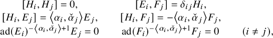 $$\begin{align*}\begin{array}{c@{\qquad}c@{\qquad}c} [H_i, H_j] = 0, & [E_i, F_j] = \delta_{ij} H_i, \\ \mbox{} [H_i, E_j] = {\left\langle {\alpha_i}, {{\check{\alpha}}_j} \right\rangle} E_j, & [H_i, F_j] = -{\left\langle {\alpha_i}, {{\check{\alpha}}_j} \right\rangle} F_j, \\ \operatorname{\mathrm{ad}}(E_i)^{-{\left\langle {\alpha_i}, {{\check{\alpha}}_j} \right\rangle} +1} E_j = 0 & \operatorname{\mathrm{ad}}(F_i)^{-{\left\langle {\alpha_i}, {{\check{\alpha}}_j} \right\rangle} +1} F_j = 0 & (i \neq j), \end{array} \end{align*}$$
where $\operatorname {\mathrm {ad}}(X) Y = [X, Y]$
is the adjoint operator. Let
$\operatorname {\mathrm {ad}}(X) Y = [X, Y]$
is the adjoint operator. Let ${\mathfrak {h}} = \operatorname {\mathrm {span}}_{{\mathbf {k}}} \{h_i\}_{i \in I}$
denote the Cartan subalgebra corresponding to T.
${\mathfrak {h}} = \operatorname {\mathrm {span}}_{{\mathbf {k}}} \{h_i\}_{i \in I}$
denote the Cartan subalgebra corresponding to T.
A representation of a Lie algebra V is a vector space over ${\mathbf {k}}$
such that
${\mathbf {k}}$
such that $[X, Y] v = X(Yv) - Y(Xv)$
for all
$[X, Y] v = X(Yv) - Y(Xv)$
for all $v \in V$
. For two
$v \in V$
. For two $\mathfrak {g}$
-representations V and W, their tensor product is naturally a
$\mathfrak {g}$
-representations V and W, their tensor product is naturally a $\mathfrak {g}$
-representation by
$\mathfrak {g}$
-representation by
 $$\begin{align*}X(v \otimes w) = Xv \otimes w + v \otimes Xw \end{align*}$$
for all $X \in \mathfrak {g}$
and
$X \in \mathfrak {g}$
and $v \otimes w \in V \otimes W$
. We restrict to the category of finite dimensional highest weight representations, and we let
$v \otimes w \in V \otimes W$
. We restrict to the category of finite dimensional highest weight representations, and we let $V(\lambda )$
denote the irreducible highest weight representation for the dominant integral weight
$V(\lambda )$
denote the irreducible highest weight representation for the dominant integral weight $\lambda \in P^+$
. The Weyl group action on V given by
$\lambda \in P^+$
. The Weyl group action on V given by
 $$\begin{align*}s_i = \exp(F_i) \exp(-E_i) \exp(F_i). \end{align*}$$
For any nilpotent element $X\in \mathfrak {g}$
and
$X\in \mathfrak {g}$
and $v \in V$
, we can implement
$v \in V$
, we can implement $\exp (X) v$
by finding
$\exp (X) v$
by finding $K = \min \{k \in \mathbb {Z}_{>0} \mid X^kv \neq 0\}$
and then computing
$K = \min \{k \in \mathbb {Z}_{>0} \mid X^kv \neq 0\}$
and then computing
 $$\begin{align*}\exp(X) v = \sum_{k=0}^K \frac{X^k v}{k!}. \end{align*}$$
We give an explicit realization for a minuscule representation following the construction in [Reference Oh and ScrimshawOS, Sec. 3.1.1], where we prove the analog of [Reference Oh and ScrimshawOS, Prop. 3.2, Prop. 3.3] for $\mathfrak {g}$
-representations. For the remainder of this section, let
$\mathfrak {g}$
-representations. For the remainder of this section, let $r \in I$
be such that
$r \in I$
be such that ${\left \langle {\omega _r}, {\check {\alpha }} \right \rangle } \leq 1$
for all
${\left \langle {\omega _r}, {\check {\alpha }} \right \rangle } \leq 1$
for all $\alpha \in \Phi ^+$
, which characterizes the minuscule representations
$\alpha \in \Phi ^+$
, which characterizes the minuscule representations $V(\omega _r)$
.
$V(\omega _r)$
.
A crystal for $\mathfrak {g}$
is a set B with crystal operators
$\mathfrak {g}$
is a set B with crystal operators $\widetilde {e}_i, {\widetilde {f}}_i \colon B \to B \sqcup \{0\}$
, for all
$\widetilde {e}_i, {\widetilde {f}}_i \colon B \to B \sqcup \{0\}$
, for all $i \in I$
, that satisfy certain properties and encode the action of the Chevalley generators
$i \in I$
, that satisfy certain properties and encode the action of the Chevalley generators $E_i$
and
$E_i$
and $F_i$
, respectively. Kashiwara showed [Reference KashiwaraKas1, Reference KashiwaraKas2] that all highest weight representations
$F_i$
, respectively. Kashiwara showed [Reference KashiwaraKas1, Reference KashiwaraKas2] that all highest weight representations $V(\lambda )$
have corresponding crystals
$V(\lambda )$
have corresponding crystals $B(\lambda )$
. We denote by
$B(\lambda )$
. We denote by $u_{\lambda }$
the unique highest weight element of
$u_{\lambda }$
the unique highest weight element of $B(\lambda )$
. For more information on crystals, we refer the reader to [Reference Bump and SchillingBS].
$B(\lambda )$
. For more information on crystals, we refer the reader to [Reference Bump and SchillingBS].
For a minuscule node r, let $J := I \setminus \{r\}$
, and let
$J := I \setminus \{r\}$
, and let $W_J := \langle s_i \mid i \in J \rangle $
denote the corresponding subgroup. Denote by
$W_J := \langle s_i \mid i \in J \rangle $
denote the corresponding subgroup. Denote by $W^J$
the set of minimal length coset representatives of
$W^J$
the set of minimal length coset representatives of $W / W_J$
. Define crystal operators
$W / W_J$
. Define crystal operators $\widetilde {e}_i, {\widetilde {f}}_i \colon W^J \to W^J \sqcup \{0\}$
by
$\widetilde {e}_i, {\widetilde {f}}_i \colon W^J \to W^J \sqcup \{0\}$
by
 $$\begin{align*}\widetilde{e}_i w = \begin{cases} s_i w & \text{if } \ell(s_i w) < \ell(w) \\ 0 & \text{otherwise}, \end{cases} \qquad\quad {\widetilde{f}}_i w = \begin{cases} s_i w & \text{if } \ell(s_i w)> \ell(w) \text{ and } s_i w \in W^J \\ 0 & \text{otherwise}, \end{cases} \end{align*}$$
and weight function $\operatorname {\mathrm {wt}}(w) = \omega _r - \alpha _{i_1} - \cdots - \alpha _{i_{\ell }}$
, where
$\operatorname {\mathrm {wt}}(w) = \omega _r - \alpha _{i_1} - \cdots - \alpha _{i_{\ell }}$
, where $s_{i_1} \cdots s_{i_{\ell }}$
is any reduced expression for
$s_{i_1} \cdots s_{i_{\ell }}$
is any reduced expression for $w \in W^J$
. By Stembridge [Reference StembridgeSt2], this is well defined, and this gives
$w \in W^J$
. By Stembridge [Reference StembridgeSt2], this is well defined, and this gives $W^J$
the structure of a crystal associated to the minuscule representation
$W^J$
the structure of a crystal associated to the minuscule representation $V(\omega _r)$
[Reference ScrimshawScr].
$V(\omega _r)$
[Reference ScrimshawScr].
Now we give an explicit construction of the minuscule representation.Footnote 1
Proposition A.1. Consider the vector space
 $$\begin{align*}\mathbb{V}(\omega_r) := \operatorname{\mathrm{span}}_{{\mathbf{k}}} \{ v_w \mid w \in W^J \}. \end{align*}$$
Then $\mathbb {V}(\omega _r)$
is made into a
$\mathbb {V}(\omega _r)$
is made into a $\mathfrak {g}$
-representation by
$\mathfrak {g}$
-representation by
 $$\begin{align*}e_i v_w = v_{\widetilde{e}_i w}, \qquad\qquad f_i v_w = v_{{\widetilde{f}}_i w}, \qquad\qquad h_i v_w = {\left\langle {\operatorname{\mathrm{wt}}(w)}, {h_i} \right\rangle} v_w, \qquad\qquad \end{align*}$$
where $v_0 = 0$
, and extended by linearity. Furthermore,
$v_0 = 0$
, and extended by linearity. Furthermore, $\mathbb {V}(\omega _r) \cong V(\omega _r)$
as
$\mathbb {V}(\omega _r) \cong V(\omega _r)$
as $\mathfrak {g}$
-representations.
$\mathfrak {g}$
-representations.
A.2 Implementation
We now give our implementation using SageMath. For our crystals, we will use the realization using rigged configurations [Reference SchillingSch, Reference Salisbury and ScrimshawSS].
We build the minuscule representation $V(\omega _1)$
in type
$V(\omega _1)$
in type $E_6$
, which is constructed as
$E_6$
, which is constructed as $\mathbb {V}(\omega _1)$
:
$\mathbb {V}(\omega _1)$
:

Let v denote the highest weight vector of $V(\omega _1)$
. There exists a highest weight vector
$V(\omega _1)$
. There exists a highest weight vector $v_{\omega _4}$
of weight
$v_{\omega _4}$
of weight $\omega _4$
in
$\omega _4$
in $V(\omega _1)^{\otimes 3}$
. Explicitly, it is given as
$V(\omega _1)^{\otimes 3}$
. Explicitly, it is given as
 $$ \begin{align*} v_{\omega_4} & = v \otimes f_1 v \otimes f_3 f_1 v - f_1 v \otimes v \otimes f_3 f_1 v - v \otimes f_3 f_1 v \otimes f_1 v \\ & \hspace{20pt} + f_1 v \otimes f_3 f_1 v \otimes v + f_3 f_1 v \otimes v \otimes f_1 v - f_3 f_1 v \otimes f_1 v \otimes v. \end{align*} $$
It is a finite computation to show this is a highest weight vector. We also perform this computation in SageMath:
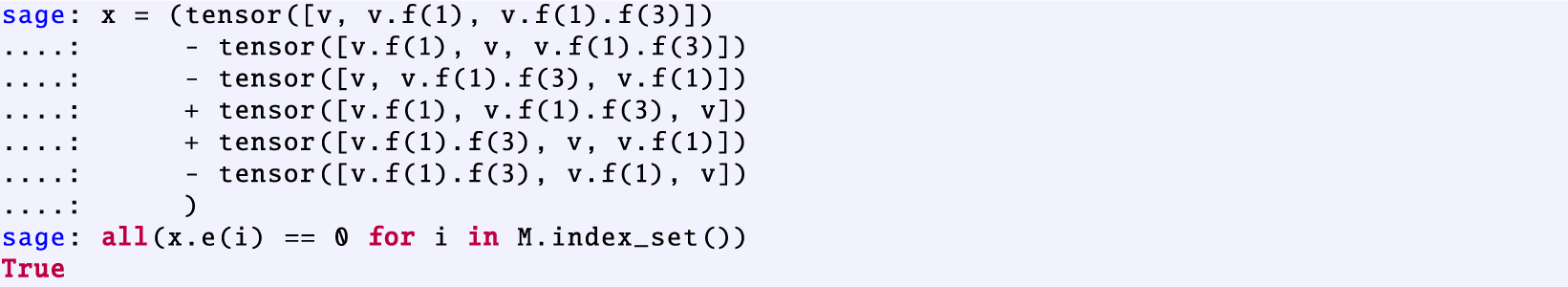
Thus, we can build a $\mathfrak {g}$
-representation by
$\mathfrak {g}$
-representation by $\mathbb {V}(\omega _4) := \langle v_{\omega _4} \rangle \subseteq V(\omega _1)^{\otimes 3}$
, and since the decomposition of tensor products of finite dimensional
$\mathbb {V}(\omega _4) := \langle v_{\omega _4} \rangle \subseteq V(\omega _1)^{\otimes 3}$
, and since the decomposition of tensor products of finite dimensional $\mathfrak {g}$
-representations is determined by computing highest weight vectors, we have
$\mathfrak {g}$
-representations is determined by computing highest weight vectors, we have $\mathbb {V}(\omega _4) \cong V(\omega _4)$
. In order to do computations, we need to construct a weight basis for
$\mathbb {V}(\omega _4) \cong V(\omega _4)$
. In order to do computations, we need to construct a weight basis for $\mathbb {V}(\omega _4)$
. We do so by using the crystal
$\mathbb {V}(\omega _4)$
. We do so by using the crystal $B(\omega _4)$
. Let
$B(\omega _4)$
. Let $b \in B(\omega _4)$
, and then define
$b \in B(\omega _4)$
, and then define $v_b = f_{i_1} \cdots f_{i_{\ell }} v_{\omega _4}$
, where
$v_b = f_{i_1} \cdots f_{i_{\ell }} v_{\omega _4}$
, where $b = {\widetilde {f}}_{i_1} \cdots {\widetilde {f}}_{i_{\ell }} u_{\omega _4}$
for some fixed path
$b = {\widetilde {f}}_{i_1} \cdots {\widetilde {f}}_{i_{\ell }} u_{\omega _4}$
for some fixed path $(i_1, \dotsc , i_{\ell })$
. Define
$(i_1, \dotsc , i_{\ell })$
. Define ${\mathcal {B}} := \{v_b \mid b \in B(\omega _4)\}$
. Clearly, this may depend on the choice of path from
${\mathcal {B}} := \{v_b \mid b \in B(\omega _4)\}$
. Clearly, this may depend on the choice of path from $u_{\omega _4} \to b$
, but regardless of this choice, we have
$u_{\omega _4} \to b$
, but regardless of this choice, we have $v_b \in V(\omega _4)_{\operatorname {\mathrm {wt}}(b)}$
.
$v_b \in V(\omega _4)_{\operatorname {\mathrm {wt}}(b)}$
.
Below, we construct $\mathbb {V}(\omega _4)$
in SageMath by using
$\mathbb {V}(\omega _4)$
in SageMath by using ${\mathcal {B}}$
as follows. For each
${\mathcal {B}}$
as follows. For each $b \in B(\omega _4)$
, we take the path recursively constructed by taking the minimal
$b \in B(\omega _4)$
, we take the path recursively constructed by taking the minimal $i_k$
such that we have a path to b from
$i_k$
such that we have a path to b from $f_{i_k} \cdots f_{i_{\ell }} u _{\omega _4}$
(although any such path could do). This gives us a set of elements
$f_{i_k} \cdots f_{i_{\ell }} u _{\omega _4}$
(although any such path could do). This gives us a set of elements ${\mathcal {B}}$
, and we need to show that
${\mathcal {B}}$
, and we need to show that ${\mathcal {B}}$
are linearly independent. We verify this by seeing the rank of the matrix of these vectors is
${\mathcal {B}}$
are linearly independent. We verify this by seeing the rank of the matrix of these vectors is $2925 = \dim V(\omega _4) = {\lvert {B(\omega _4)} \rvert }$
. Furthermore, we verify that this does give us a
$2925 = \dim V(\omega _4) = {\lvert {B(\omega _4)} \rvert }$
. Furthermore, we verify that this does give us a $\mathfrak {g}$
-representation by checking all of the relations are satisfied on each basis element:
$\mathfrak {g}$
-representation by checking all of the relations are satisfied on each basis element:

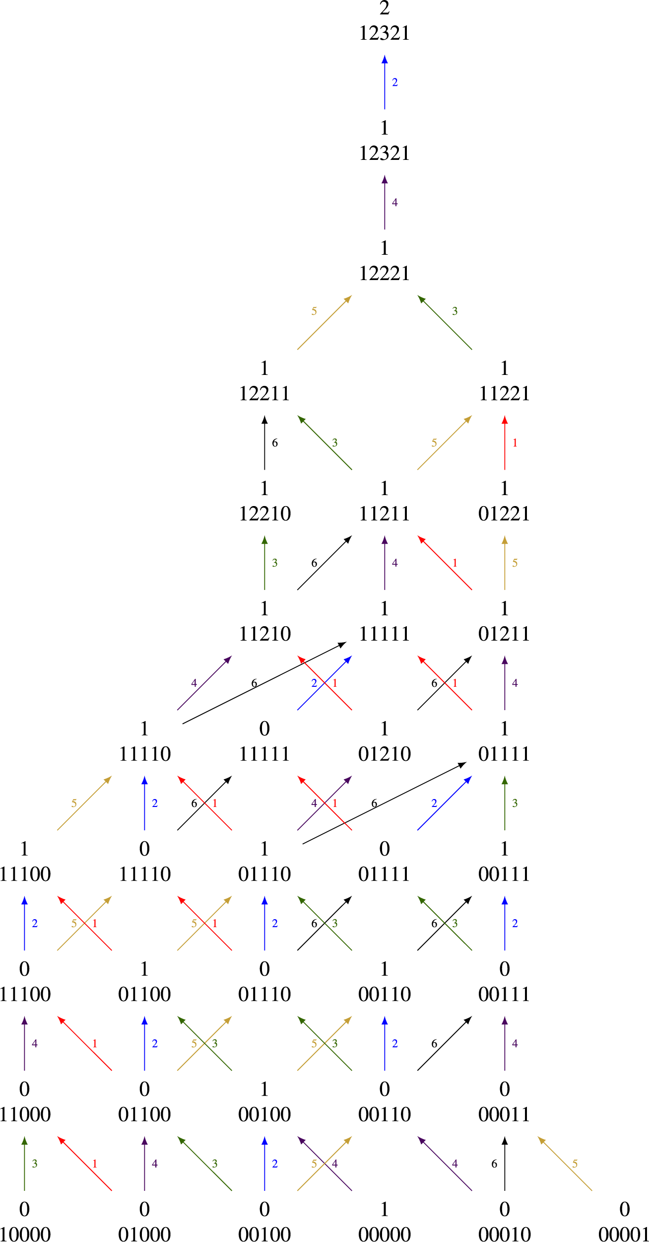
Figure 3 The root poset $\Phi ^+$
in type
$\Phi ^+$
in type $E_6$
.
$E_6$
.
Next, consider the positive roots
 $$ \begin{align*} \beta& = \alpha_1 + \alpha_2 + 2 \alpha_3 + 3 \alpha_4 + 2 \alpha_5 + \alpha_6 = \begin{array}{c@{}c@{}c@{}c@{}c} &&1\\ 1&2&3&2&1 \end{array}, \\ \theta & = \alpha_1 + 2\alpha_2 + 2 \alpha_3 + 3 \alpha_4 + 2 \alpha_5 + \alpha_6 = \begin{array}{c@{}c@{}c@{}c@{}c} &&2\\ 1&2&3&2&1 \end{array}. \end{align*} $$
Since all of the root spaces in $\mathfrak {g}$
are 1-dimensional (that is,
$\mathfrak {g}$
are 1-dimensional (that is, $\dim \mathfrak {g}_{\alpha } = 1$
for all
$\dim \mathfrak {g}_{\alpha } = 1$
for all $\alpha \in \Phi $
), we construct the basis element
$\alpha \in \Phi $
), we construct the basis element $f_{\gamma }$
of
$f_{\gamma }$
of $\mathfrak {g}_{\gamma }$
(which forms the unique basis up to scalar) by finding some sequence
$\mathfrak {g}_{\gamma }$
(which forms the unique basis up to scalar) by finding some sequence $(i_1, i_2, \dotsc , i_{\ell })$
such that
$(i_1, i_2, \dotsc , i_{\ell })$
such that
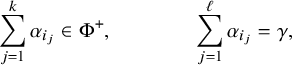 $$\begin{align*}\sum_{j=1}^k \alpha_{i_j} \in \Phi^+, \qquad\qquad \sum_{j=1}^{\ell} \alpha_{i_j} = \gamma, \end{align*}$$
for all $1 \leq k \leq \ell $
. In particular, we can take any path from
$1 \leq k \leq \ell $
. In particular, we can take any path from $\alpha _{i_1}$
to
$\alpha _{i_1}$
to $\gamma $
in Figure 3. Then we have
$\gamma $
in Figure 3. Then we have
 $$\begin{align*}f_{\gamma} = [\cdots[[f_{i_1}, f_{i_2}], f_{i_3}] \cdots f_{i_{\ell}}]. \end{align*}$$
We write $f_{\gamma }$
in the free algebra generated by
$f_{\gamma }$
in the free algebra generated by $\langle f_i \rangle _{i \in I}$
using the commutator property
$\langle f_i \rangle _{i \in I}$
using the commutator property $[X, Y] = XY - YX$
and apply the result to any vector in the
$[X, Y] = XY - YX$
and apply the result to any vector in the $\mathfrak {g}$
-representation. In other words, we compute
$\mathfrak {g}$
-representation. In other words, we compute
 $$\begin{align*}f_{\gamma} = \sum_{\mathbf{a}} \pm f_{a_1} \cdots f_{a_{\ell-1}} f_{a_{\ell}}, \qquad\qquad f_{\gamma} v = \sum_{\mathbf{a}} \pm (f_{a_1} \cdots (f_{a_{\ell-1}} (f_{a_{\ell}} v)) \cdots). \end{align*}$$
Using this process, we construct the vector $v = f_{\theta } f_{\beta } v_{\omega _4}$
:
$v = f_{\theta } f_{\beta } v_{\omega _4}$
:
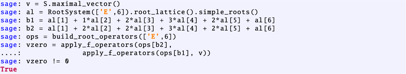
Lastly, we construct the orbit up to sign and show that it spans a $45$
-dimensional vector space:
$45$
-dimensional vector space:
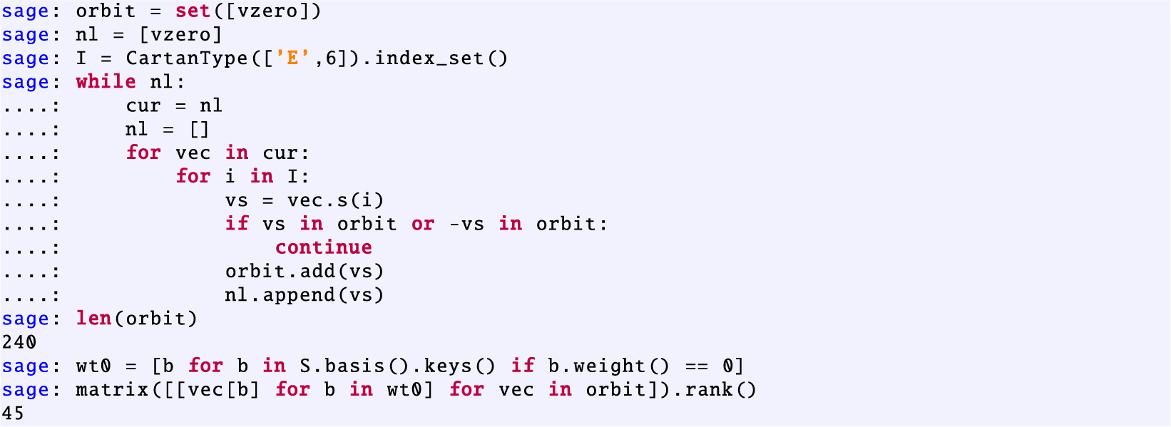
Remark A.1. The SageMath code for the implementation in this appendix is included as an ancillary file on arXiv:2010.11357.
Acknowledgements
M. Besson and J. Hong would like to thank the hospitality of Max Planck Institute for Mathematics at Bonn during our visits in November and December of 2019, where part of the work was done. They also would like to thank Thomas Haines, Timo Richarz, Michael Strayer and Xinwen Zhu for helpful conversations and valuable comments.
Competing interest
The authors have no competing interests to declare.
Funding statement
J. Hong is partially supported by the Simons collaboration Grant 524406 and NSF grant DMS-2001365.


 Open access