


1 Introduction
Let $X_{N}=\left\{ x_{1},\ldots , x_N \right\}$
be a set of variables. The Macdonald polynomials
$X_{N}=\left\{ x_{1},\ldots , x_N \right\}$
be a set of variables. The Macdonald polynomials $\left\{ P_{\lambda }[X_N;q,t] \right\}$
are a basis of the ring of
$\left\{ P_{\lambda }[X_N;q,t] \right\}$
are a basis of the ring of $(q,t)$
-deformed symmetric polynomials
$(q,t)$
-deformed symmetric polynomials $\mathbb {Q}(q,t)[X_N]^{\mathfrak {S}_N}$
that have appeared across a remarkably broad collection of mathematical fields. They can be characterized as eigenfunctions of a commuting family of difference operators, the Macdonald operators: for
$\mathbb {Q}(q,t)[X_N]^{\mathfrak {S}_N}$
that have appeared across a remarkably broad collection of mathematical fields. They can be characterized as eigenfunctions of a commuting family of difference operators, the Macdonald operators: for $1\le n\le N$
,
$1\le n\le N$
,
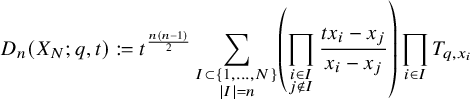 $$ \begin{align} D_n(X_N ;q,t)&:=t^{\frac{n(n-1)}{2}}\sum_{\substack{I\subset\{1,\ldots, N\}\\ |I|=n}}\left(\prod_{\substack{i\in I\\j\not\in I}}\frac{tx_i-x_j}{x_i-x_j}\right)\prod_{i\in I} T_{q,x_i} \end{align} $$
 $$ \begin{align} D_n(X_N ;q,t) P_{\lambda}[X_N;q,t] &= e_n(q^{\lambda_1}t^{N-1}, q^{\lambda_2}t^{N-2},\ldots, q^{\lambda_N})P_{\lambda}[X_N ;q,t]. \end{align} $$
Here, $T_{q,x_i}$
is the q-shift operator
$T_{q,x_i}$
is the q-shift operator
 $$\begin{align*}T_{q,x_i} x_j=q^{\delta_{i,j}}x_j \end{align*}$$
and $e_n$
is the nth elementary symmetric polynomial. The Macdonald operators are themselves distinguished as Hamiltonians of the quantum trigonometric Ruijsenaars-Schneider integrable system.
$e_n$
is the nth elementary symmetric polynomial. The Macdonald operators are themselves distinguished as Hamiltonians of the quantum trigonometric Ruijsenaars-Schneider integrable system.
This paper is concerned with the wreath Macdonald polynomials, a generalization of the Macdonald polynomials proposed by Haiman [Reference Haiman7]. Fix an integer $r>0$
and partition the variables
$r>0$
and partition the variables $x_1,\ldots , x_N$
into r subsets:
$x_1,\ldots , x_N$
into r subsets:
 $$\begin{align*}X_{N_{\bullet}}:=\bigsqcup_{i=0}^{r-1}\left\{x^{(i)}_{l}\right\}_{l=1,\ldots, N_i}=\left\{ x_1,\ldots,x_N \right\} \end{align*}$$
where $\sum _{i=0}^{r-1}N_i=N$
. We call the index i the color of
$\sum _{i=0}^{r-1}N_i=N$
. We call the index i the color of $x^{(i)}_{l}$
, and it will be helpful to view it as an element of
$x^{(i)}_{l}$
, and it will be helpful to view it as an element of $I:=\mathbb {Z}/r\mathbb {Z}$
. The number of variables is recorded by the vector
$I:=\mathbb {Z}/r\mathbb {Z}$
. The number of variables is recorded by the vector $N_{\bullet } :=(N_0,\ldots , N_{r-1})$
, and we set
$N_{\bullet } :=(N_0,\ldots , N_{r-1})$
, and we set $|N_{\bullet }|:=N$
. Consider the action of the product of symmetric groups
$|N_{\bullet }|:=N$
. Consider the action of the product of symmetric groups
 $$\begin{align*}\mathfrak{S}_{N_{\bullet}}:=\prod_{i\in I}\mathfrak{S}_{N_i} \end{align*}$$
on the polynomial ring $\mathbb {Q}(q,t)\left[ X_{N_{\bullet }} \right]$
whereby
$\mathbb {Q}(q,t)\left[ X_{N_{\bullet }} \right]$
whereby $\mathfrak {S}_{N_i}$
only permutes the variables of color i. The wreath Macdonald polynomials can be viewed as a set of color-symmetric polynomials that are again indexed by a single partition:
$\mathfrak {S}_{N_i}$
only permutes the variables of color i. The wreath Macdonald polynomials can be viewed as a set of color-symmetric polynomials that are again indexed by a single partition:
 $$\begin{align*}P_{\lambda}[X_{N_{\bullet}};q,t]\in\mathbb{Q}(q,t)\left[ X_{N_{\bullet}} \right]^{\mathfrak{S}_{N_{\bullet}}}. \end{align*}$$
The combinatorics of r-cores and r-quotients play a key role in this subject, which we review in Section 2 below. When we restrict $\lambda $
to range over partitions with a fixed r-core and
$\lambda $
to range over partitions with a fixed r-core and $\ell (\lambda )\le |N_{\bullet }|$
, we obtain a basis of color-symmetric polynomials. For reasons that seem technical at first, the r-core and
$\ell (\lambda )\le |N_{\bullet }|$
, we obtain a basis of color-symmetric polynomials. For reasons that seem technical at first, the r-core and $N_{\bullet }$
must satisfy a compatibility condition (see 2.9). The original Macdonald polynomials are the case
$N_{\bullet }$
must satisfy a compatibility condition (see 2.9). The original Macdonald polynomials are the case $r=1$
.
$r=1$
.
Haiman’s proposed definition characterizes $P_{\lambda }[X_{N_{\bullet }};q,t]$
using a pair of triangularity conditions. In contrast with the usual Macdonald theory, we a priori do not have an analogous characterization as the joint eigenfunction of an explicit family of difference operators. The present work remedies this situation: we produce a novel family of difference-permutation operators that are diagonalized by the wreath Macdonald polynomials and whose eigenvalues are written in terms of the elementary symmetric polynomials. In addition to the degree n, they also carry a color parameter
$P_{\lambda }[X_{N_{\bullet }};q,t]$
using a pair of triangularity conditions. In contrast with the usual Macdonald theory, we a priori do not have an analogous characterization as the joint eigenfunction of an explicit family of difference operators. The present work remedies this situation: we produce a novel family of difference-permutation operators that are diagonalized by the wreath Macdonald polynomials and whose eigenvalues are written in terms of the elementary symmetric polynomials. In addition to the degree n, they also carry a color parameter $p\in I$
:
$p\in I$
:
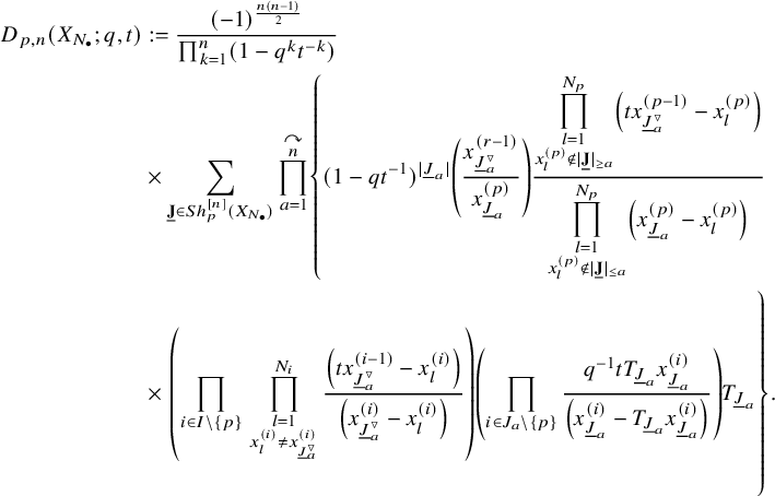 $$ \begin{align} \begin{aligned} D_{p,n}(X_{N_{\bullet}};q,t)&:= \frac{(-1)^{\frac{n(n-1)}{2}}}{\prod_{k=1}^n(1-q^{k}t^{-k})}\\ &\times\sum_{\mathbf{{\underline{J}}}\in Sh_p^{[n]}(X_{N_{\bullet}})} \overset{\curvearrowright}{\prod_{a=1}^n} \left\{(1-qt^{-1})^{|{\underline{J}}_a|}\left(\frac{x^{(r-1)}_{{\underline{J}}_a^\triangledown}}{x^{(p)}_{{\underline{J}}_a}}\right) \frac{\displaystyle \prod_{\substack{l=1\\x^{(p)}_{l}\not\in|\mathbf{{\underline{J}}}|_{\ge a}}}^{N_p}\left( tx^{(p-1)}_{{\underline{J}}_a^\triangledown}-x^{(p)}_{l} \right)} {\displaystyle \prod_{\substack{l=1\\x^{(p)}_{l}\not\in|\mathbf{{\underline{J}}}|_{\le a}}}^{N_p}\left( x^{(p)}_{{\underline{J}}_a}-x^{(p)}_{l} \right)}\right.\\ &\times \left. \left( \prod_{\substack{i\in I\backslash\{p\}}}\, \prod_{\substack{l=1\\x^{(i)}_{l}\not=x^{(i)}_{{\underline{J}}_a^\triangledown}}}^{N_i}\frac{\left(tx^{(i-1)}_{{\underline{J}}_a^\triangledown}-x^{(i)}_{l}\right)} {\left( x^{(i)}_{{\underline{J}}_a^\triangledown}-x^{(i)}_{l} \right)} \right) \left( \prod_{i\in J_a\backslash \left\{ p \right\}} \frac{q^{-1}t T_{{\underline{J}}_a}x^{(i)}_{{\underline{J}}_a}} {\left( x^{(i)}_{{\underline{J}}_a}-T_{{\underline{J}}_a}x^{(i)}_{{\underline{J}}_a} \right)} \right) T_{{\underline{J}}_a}\vphantom{\frac{\displaystyle \prod_{\substack{l=1\\x^{(p)}_{l}\not\in|\mathbf{{\underline{J}}}|_{\ge a}}}^{N_p}\left( tx^{(p-1)}_{{\underline{J}}_a^\triangledown}-x^{(p)}_{l} \right)} {\displaystyle \prod_{\substack{l=1\\x^{(p)}_{l}\not\in|\mathbf{{\underline{J}}}|_{\le a}}}^{N_p}\left( x^{(p)}_{{\underline{J}}_a}-x^{(p)}_{l} \right)}}\right\}. \end{aligned} \end{align} $$
The notation used in this formula is outlined in 5.1.4. Our main result is the following:
Theorem (see Theorem 5.21)
For $\lambda $
having r-core compatible with
$\lambda $
having r-core compatible with $N_{\bullet }$
and
$N_{\bullet }$
and $\ell (\lambda )\le |N_{\bullet }|$
, the polynomial
$\ell (\lambda )\le |N_{\bullet }|$
, the polynomial $P_{\lambda }[X_{N_{\bullet }};q,t]$
satisfies the eigenfunction equation
$P_{\lambda }[X_{N_{\bullet }};q,t]$
satisfies the eigenfunction equation
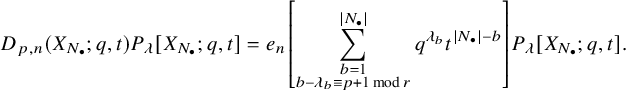 $$ \begin{align} D_{p,n}(X_{N_{\bullet}};q,t)P_{\lambda}[X_{N_{\bullet}};q,t] =e_n\left[ \sum_{\substack{b=1\\ b-\lambda_b\equiv p+1\: \mathrm{mod} \: r}}^{|N_{\bullet}|}q^{\lambda_b}t^{|N_{\bullet}|-b} \right] P_{\lambda}[X_{N_{\bullet}};q,t]. \end{align} $$
For the eigenvalues, we have used plethystic notation – we merely mean the elementary symmetric function $e_n$
evaluated at the characters appearing in the summation. In earlier work [Reference Orr and Shimozono14], the first two authors constructed the first order dual operators
$e_n$
evaluated at the characters appearing in the summation. In earlier work [Reference Orr and Shimozono14], the first two authors constructed the first order dual operators $D_{p,1}^*$
and their eigenfunction equation in Theorem 5.21.
$D_{p,1}^*$
and their eigenfunction equation in Theorem 5.21.
Our operators (1.3) are much more complicated than the original Macdonald operators (1.1). In the case $r=1$
, we do indeed obtain (1.1) after some simplification (see Remark 5.15). When
$r=1$
, we do indeed obtain (1.1) after some simplification (see Remark 5.15). When $r>1$
, the vanilla q-shift operator
$r>1$
, the vanilla q-shift operator $T_{q,x_i}$
is replaced with what we call a cyclic-shift operator
$T_{q,x_i}$
is replaced with what we call a cyclic-shift operator $T_{{\underline {J}}_a}$
, which cyclically permutes variables of different colors in addition to multiplying by a power of q. Because of this extra permutation, the cyclic-shift operators might not commute. Note now the ordered product in (1.3) – we expect the formula to simplify meaningfully after taking into account the (non)commutativity of the constituent cyclic-shift operators. Moving beyond the intricacies of our formula, let us now highlight some nice conceptual aspects of our operators.
$T_{{\underline {J}}_a}$
, which cyclically permutes variables of different colors in addition to multiplying by a power of q. Because of this extra permutation, the cyclic-shift operators might not commute. Note now the ordered product in (1.3) – we expect the formula to simplify meaningfully after taking into account the (non)commutativity of the constituent cyclic-shift operators. Moving beyond the intricacies of our formula, let us now highlight some nice conceptual aspects of our operators.
1.1 Integral formulas
Our strategy for deriving (1.3) and establishing the eigenfunction equation uses work of the third author [Reference Wen19]. Namely, we study the wreath Macdonald polynomials using the quantum toroidal algebra $U_{\mathfrak {q},\mathfrak {d}}(\ddot {\mathfrak {sl}}_r)$
and its vertex representation W. The aforementioned work proves that infinite-variable wreath Macdonald polynomials can be naturally embedded inside W such that they diagonalize a large commutative subalgebra of
$U_{\mathfrak {q},\mathfrak {d}}(\ddot {\mathfrak {sl}}_r)$
and its vertex representation W. The aforementioned work proves that infinite-variable wreath Macdonald polynomials can be naturally embedded inside W such that they diagonalize a large commutative subalgebra of $U_{\mathfrak {q},\mathfrak {d}}(\ddot {\mathfrak {sl}}_r)$
, the horizontal Heisenberg subalgebra. This alone is insufficient for obtaining explicit formulas – we also need work of Neguţ [Reference Neguţ11] realizing
$U_{\mathfrak {q},\mathfrak {d}}(\ddot {\mathfrak {sl}}_r)$
, the horizontal Heisenberg subalgebra. This alone is insufficient for obtaining explicit formulas – we also need work of Neguţ [Reference Neguţ11] realizing $U_{\mathfrak {q},\mathfrak {d}}(\ddot {\mathfrak {sl}}_r)$
in terms of a shuffle algebra. The shuffle algebra is a space of rational functions endowed with an exotic product structure, and it is isomorphic to a part of
$U_{\mathfrak {q},\mathfrak {d}}(\ddot {\mathfrak {sl}}_r)$
in terms of a shuffle algebra. The shuffle algebra is a space of rational functions endowed with an exotic product structure, and it is isomorphic to a part of $U_{\mathfrak {q},\mathfrak {d}}(\ddot {\mathfrak {sl}}_r)$
via a map that is morally (but not precisely) an integration map. Writing its action on W and then specializing from infinite to finite variables, we obtain actual integral formulas. Finally, to pin down the eigenvalues, we use the (twisted) isomorphism established by Tsymbaliuk [Reference Tsymbaliuk17] between the vertex representation and the Fock representation.
$U_{\mathfrak {q},\mathfrak {d}}(\ddot {\mathfrak {sl}}_r)$
via a map that is morally (but not precisely) an integration map. Writing its action on W and then specializing from infinite to finite variables, we obtain actual integral formulas. Finally, to pin down the eigenvalues, we use the (twisted) isomorphism established by Tsymbaliuk [Reference Tsymbaliuk17] between the vertex representation and the Fock representation.
We apply this process to the shuffle realizations of well-chosen elements of the horizontal Heisenberg subalgebra which were found in [Reference Wen19]. Our operators are the highest degree parts (see Proposition 5.16), and we can write their action as follows: for a factored element
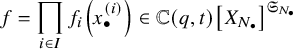 $$\begin{align*}f=\prod_{i\in I} f_i\left(x^{(i)}_{\bullet}\right)\in\mathbb{C}(q,t)\left[ X_{N_{\bullet}} \right]^{\mathfrak{S}_{N_{\bullet}}} \end{align*}$$
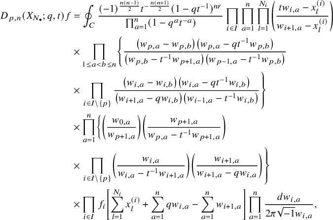 $$ \begin{align*} D_{p,n}(X_{N_{\bullet}};q,t)f&= \oint_{C} \frac{(-1)^{\frac{n(n-1)}{2}}t^{-\frac{n(n+1)}{2}}(1-qt^{-1})^{nr}}{\prod_{a=1}^n(1-q^at^{-a})} \prod_{i\in I}\prod_{a=1}^n\prod_{l=1}^{N_i}\left(\frac{ tw_{i,a}-x^{(i)}_{l} }{ w_{i+1,a}-x^{(i)}_{l} }\right)\\ &\times\prod_{1\le a<b\le n}\left\{ \frac{\left(w_{p,a}-w_{p,b}\right)\left(w_{p,a}-qt^{-1}w_{p,b}\right)}{\left(w_{p,b}-t^{-1}w_{p+1,a}\right)\left(w_{p-1,a}-t^{-1}w_{p,b}\right)}\right.\\ &\times\left. \prod_{i\in I\backslash\{p\}} \frac{\left(w_{i,a}-w_{i,b}\right)\left(w_{i,a}-qt^{-1}w_{i,b}\right)}{\left(w_{i+1,a}-qw_{i,b}\right)\left(w_{i-1,a}-t^{-1}w_{i,b}\right)}\right\}\\ &\times \prod_{a=1}^n\left\{ \left(\frac{w_{0,a}}{w_{p+1,a}}\right)\left(\frac{w_{p+1,a}}{w_{p,a}-t^{-1}w_{p+1,a}}\right)\right.\\ &\times\left. \prod_{i\in I\setminus\{p\}} \left(\frac{w_{i,a}}{w_{i,a}-t^{-1}w_{i+1,a}}\right) \left( \frac{w_{i+1,a}}{w_{i+1,a}-qw_{i,a}} \right) \right\}\\ &\times \prod_{i\in I}f_i\left[ \sum_{l=1}^{N_i}x^{(i)}_{l}+\sum_{a=1}^nqw_{i,a}-\sum_{a=1}^nw_{i+1,a} \right] \prod_{a=1}^n \frac{dw_{i,a}}{2\pi\sqrt{-1}w_{i,a}}, \end{align*} $$
where for each variable $w_{i,a}$
, the cycle C only encloses poles of the form
$w_{i,a}$
, the cycle C only encloses poles of the form $(w_{i,a}-qw_{i-1,b})$
and
$(w_{i,a}-qw_{i-1,b})$
and $(w_{i,a}-x_{i-1,l})$
. Explicit evaluation of this integral leads to (1.4). We also carry this out for its dual counterpart in Theorem 5.21.
$(w_{i,a}-x_{i-1,l})$
. Explicit evaluation of this integral leads to (1.4). We also carry this out for its dual counterpart in Theorem 5.21.
Using other shuffle elements from [Reference Wen19], we obtain similar integral formulas for wreath analogues of the Noumi-Sano operators [Reference Noumi and Sano12], although we are only able to evaluate the integral and obtain formulas for the operators in degree $n=1$
. We note that our approach is similar to [Reference Feigin, Hashizume, Hoshino, Shiraishi and Yanagida4] in the
$n=1$
. We note that our approach is similar to [Reference Feigin, Hashizume, Hoshino, Shiraishi and Yanagida4] in the $r=1$
case, although our a priori knowledge and endgoals are different. In [Reference Feigin, Hashizume, Hoshino, Shiraishi and Yanagida4], the authors use the well-known Macdonald operators to study the action of certain shuffle elements, whereas we use
$r=1$
case, although our a priori knowledge and endgoals are different. In [Reference Feigin, Hashizume, Hoshino, Shiraishi and Yanagida4], the authors use the well-known Macdonald operators to study the action of certain shuffle elements, whereas we use $r>1$
analogues of their shuffle elements to discover new operators. In [Reference Tsymbaliuk18], Tsymbaliuk has also produced difference operators out of
$r>1$
analogues of their shuffle elements to discover new operators. In [Reference Tsymbaliuk18], Tsymbaliuk has also produced difference operators out of $U_{\mathfrak {q},\mathfrak {d}}(\ddot {\mathfrak {sl}}_r)$
through very different means. The relation between Tsymbaliuk’s operators to wreath Macdonald theory does not seem straightforward but could be interesting.
$U_{\mathfrak {q},\mathfrak {d}}(\ddot {\mathfrak {sl}}_r)$
through very different means. The relation between Tsymbaliuk’s operators to wreath Macdonald theory does not seem straightforward but could be interesting.
1.2 Towards bispectral duality
In the case $r=1$
, the eigenfunction equation (1.2) is particularly interesting when juxtaposed with the Pieri rules [Reference Macdonald9]. To make this apparent, introduce a continuous extension of the discrete parameters
$r=1$
, the eigenfunction equation (1.2) is particularly interesting when juxtaposed with the Pieri rules [Reference Macdonald9]. To make this apparent, introduce a continuous extension of the discrete parameters $\lambda =(\lambda _1,\ldots ,\lambda _{N})$
:
$\lambda =(\lambda _1,\ldots ,\lambda _{N})$
:
 $$\begin{align*}s_i:=q^{\lambda_i}t^{N-i},\, S_N:=\{s_1,\ldots, s_N\}. \end{align*}$$
We call the variables $X_N$
the position variables and
$X_N$
the position variables and $S_N$
the spectral variables. It is natural to interpret the spectral q-shift
$S_N$
the spectral variables. It is natural to interpret the spectral q-shift $T_{q,s_i}P_{\lambda }[X_N;q,t]$
as adding a box to row i of the partition
$T_{q,s_i}P_{\lambda }[X_N;q,t]$
as adding a box to row i of the partition $\lambda $
. For a certain renormalization
$\lambda $
. For a certain renormalization $\tilde {P}_{\lambda }[X_N;q,t]$
of
$\tilde {P}_{\lambda }[X_N;q,t]$
of $P_{\lambda }[X_{N};,q,t]$
, we can write the Pieri rules as
$P_{\lambda }[X_{N};,q,t]$
, we can write the Pieri rules as
 $$ \begin{align} e_n(x_1,\ldots, x_N)\tilde{P}_{\lambda}[X_N ;q,t] =t^{\frac{n(n-1)}{2}}\sum_{\substack{I\subset\{1,\ldots, N\}\\|I|=n}}\left(\prod_{\substack{i\in I\\j\not\in I}}\frac{ts_i-s_j}{s_i-s_j}\right)\prod_{i\in I} T_{q,s_i}\tilde{P}_{\lambda}[X_{N} ;q,t]. \end{align} $$
The fact that no shift operator $T_{q,s_i}$
appears more than once enforces the well-known support condition of the Pieri rules: the
$T_{q,s_i}$
appears more than once enforces the well-known support condition of the Pieri rules: the $\tilde {P}_\mu [X_N;q,t]$
that appear on the right-hand side of (1.5) are such that
$\tilde {P}_\mu [X_N;q,t]$
that appear on the right-hand side of (1.5) are such that $\mu \backslash \lambda $
contains no horizontally adjacent boxes. However, we can view the eigenfunction equation (1.2) as describing multiplication by
$\mu \backslash \lambda $
contains no horizontally adjacent boxes. However, we can view the eigenfunction equation (1.2) as describing multiplication by $e_n(s_1,\ldots , s_N)$
. The similarity between (1.2) and (1.5) is reflective of a symmetry
$e_n(s_1,\ldots , s_N)$
. The similarity between (1.2) and (1.5) is reflective of a symmetry $X_N\leftrightarrow S_N$
.
$X_N\leftrightarrow S_N$
.
This symmetry is the subject of many beautiful works in Macdonald theory. A totalizing perspective on this was given by Noumi and Shiraishi [Reference Noumi and Shiraishi13], who produced an explicit function $f_N(s_1,\ldots , s_N|x_1,\ldots , x_N)$
satisfying
$f_N(s_1,\ldots , s_N|x_1,\ldots , x_N)$
satisfying
 $$ \begin{align*} f_N(q^{\lambda_1}t^{N-1},q^{\lambda_2}t^{N-2},\ldots, q^{\lambda_N}|x_1,\ldots, x_N)&= \tilde{P}_{\lambda}[X_N;q,t]\\ f_N(s_1,\ldots, s_N|x_1,\ldots, x_N)&= f_N(x_1,\ldots, x_N|s_1,\ldots, s_N). \end{align*} $$
Discretizing the x-variables as well, we obtain the well-known evaluation duality [Reference Macdonald9]:
 $$\begin{align*}\tilde{P}_{\lambda}(q^{\mu_1}t^{N-1},q^{\mu_2}t^{N-2},\ldots, q^{\mu_N})=\tilde{P}_\mu(q^{\lambda_1}t^{N-1},q^{\lambda_2}t^{N-2},\ldots, q^{\lambda_N}). \end{align*}$$
The evaluation duality is also a consequence of the Cherednik-Macdonald-Mehta formula [Reference Cherednik2], which can be regarded as a remarkable statement about the quantum toroidal algebra $U_{q,t}(\ddot {\mathfrak {gl}}_1)$
and its Miki automorphism. The
$U_{q,t}(\ddot {\mathfrak {gl}}_1)$
and its Miki automorphism. The $X_N\leftrightarrow S_N$
symmetry has also been extended by Etingof and Varchenko [Reference Etingof and Varchenko3] to the much broader context of traces of intertwiners for quantum groups, although we note that in their setting, finding explicit formulas is difficult. Finally, the symmetry is also a case of 3d mirror symmetry as proposed by Okounkov [Reference Aganagic and Okounkov1].
$X_N\leftrightarrow S_N$
symmetry has also been extended by Etingof and Varchenko [Reference Etingof and Varchenko3] to the much broader context of traces of intertwiners for quantum groups, although we note that in their setting, finding explicit formulas is difficult. Finally, the symmetry is also a case of 3d mirror symmetry as proposed by Okounkov [Reference Aganagic and Okounkov1].
For the wreath case $r>1$
, the spectral variables should also have color. We assign
$r>1$
, the spectral variables should also have color. We assign $s^{(i)}_{l}$
to some b such that
$s^{(i)}_{l}$
to some b such that $b-\lambda _b\equiv i+1$
mod r:
$b-\lambda _b\equiv i+1$
mod r:
 $$\begin{align*}s^{(i)}_{l}:=q^{\lambda_b}t^{|N_{\bullet}|-b}. \end{align*}$$
Here, we point out a natural motivation for imposing our compatibility condition between $\mathrm {core}_r(\lambda )$
and
$\mathrm {core}_r(\lambda )$
and $N_{\bullet }$
– it forces there to also be
$N_{\bullet }$
– it forces there to also be $N_i$
spectral variables of color i. The eigenfunction equation (1.4) then describes multiplication by
$N_i$
spectral variables of color i. The eigenfunction equation (1.4) then describes multiplication by $e_n(s^{(p)}_{1},\ldots , s^{(p)}_{N_p})$
. Note that adding a box to a row will not only contribute a q-shift but also change the color, and that is precisely what the cyclic-shift operators
$e_n(s^{(p)}_{1},\ldots , s^{(p)}_{N_p})$
. Note that adding a box to a row will not only contribute a q-shift but also change the color, and that is precisely what the cyclic-shift operators $T_{{\underline {J}}_a}$
do. Work of the third author [Reference Wen19] provides one constraint on the support of the wreath Pieri rules. Namely, for a box
$T_{{\underline {J}}_a}$
do. Work of the third author [Reference Wen19] provides one constraint on the support of the wreath Pieri rules. Namely, for a box $(a,b)$
, if we call the class of
$(a,b)$
, if we call the class of $b-a$
mod r its color, then
$b-a$
mod r its color, then $P_\mu [X_{N_{\bullet }};q,t]$
appears as a summand of
$P_\mu [X_{N_{\bullet }};q,t]$
appears as a summand of
 $$\begin{align*}e_n(x_{p,1},\ldots, x_{p,N_p})P_{\lambda}[X_{N_{\bullet}};q,t] \end{align*}$$
only if $\mu \backslash \lambda $
consists of n boxes of each color such that no boxes of color p and
$\mu \backslash \lambda $
consists of n boxes of each color such that no boxes of color p and $p+1$
are horizontally adjacent. One can check that the combinations of
$p+1$
are horizontally adjacent. One can check that the combinations of $T_{{\underline {J}}_a}$
appearing in (1.3) enforce this condition after swapping
$T_{{\underline {J}}_a}$
appearing in (1.3) enforce this condition after swapping $x^{(i)}_{l}\leftrightarrow s^{(i)}_{l}$
. Computer calculations done by the second author also confirm a wreath analogue of evaluation duality. While we are still a long way from establishing a wreath analogue of the
$x^{(i)}_{l}\leftrightarrow s^{(i)}_{l}$
. Computer calculations done by the second author also confirm a wreath analogue of evaluation duality. While we are still a long way from establishing a wreath analogue of the $X_N\leftrightarrow S_N$
symmetry, our strange operators seem to go out of their way to say it must be true. Generalizing any of the aforementioned perspectives for understanding this symmetry must surely lead to interesting mathematics.
$X_N\leftrightarrow S_N$
symmetry, our strange operators seem to go out of their way to say it must be true. Generalizing any of the aforementioned perspectives for understanding this symmetry must surely lead to interesting mathematics.
1.3 Outline
Section 2 introduces the wreath Macdonald polynomials. It includes a review of the combinatorics of r-cores and r-quotients. Section 3 focuses on the quantum toroidal algebra and its representations. We derive eigenvalues for the infinite-variable analogues of our operators. Section 4 moves onto the shuffle algebra. We write the action of a shuffle element on the vertex representation as the constant term of a series. Section 5 is the technical heart of the paper. We derive integral formulas for our operators and compute the integral. Some additional efforts are needed to go from the infinite-variable eigenvalues to their finite-variable versions. Finally, in the Appendix, we derive integral formulas for wreath analogues of Noumi-Sano operators. Unfortunately, for these operators, we were only able to evaluate the integrals for degree $n=1$
. Throughout, we present examples following the derivation of each of our operators.
$n=1$
. Throughout, we present examples following the derivation of each of our operators.
2 Wreath Macdonald functions
Fix a positive integer r and let $I=\mathbb {Z}/r\mathbb {Z}$
.
$I=\mathbb {Z}/r\mathbb {Z}$
.
2.1 Partitions
Let $\mathbb {Y}$
be the set of all integer partitions. We define the diagram of a partition
$\mathbb {Y}$
be the set of all integer partitions. We define the diagram of a partition $\mu =(\mu _1,\mu _2,\dotsc )\in \mathbb {Y}$
to be
$\mu =(\mu _1,\mu _2,\dotsc )\in \mathbb {Y}$
to be $D(\mu )=\{(a,b)\in \left(\mathbb {Z}_{\ge 0}\right)^2 : 0 \le a < \mu _{b+1} \}.$
The residue of
$D(\mu )=\{(a,b)\in \left(\mathbb {Z}_{\ge 0}\right)^2 : 0 \le a < \mu _{b+1} \}.$
The residue of $(a,b)\in \mathbb {Z}^2$
is the element
$(a,b)\in \mathbb {Z}^2$
is the element $b-a\in \mathbb {Z}/r\mathbb {Z}$
.
$b-a\in \mathbb {Z}/r\mathbb {Z}$
.
2.2 Edge sequences and partitions
A function $b:\mathbb {Z}\to \{0,1\}$
can be viewed as an infinite indexed binary word
$b:\mathbb {Z}\to \{0,1\}$
can be viewed as an infinite indexed binary word $\dotsm b(1) b(0) b(-1) \dotsm $
; notice that in writing such a word, we index the positions in reverse order. An inversion of b is a pair of integers
$\dotsm b(1) b(0) b(-1) \dotsm $
; notice that in writing such a word, we index the positions in reverse order. An inversion of b is a pair of integers $i>j$
such that
$i>j$
such that $b(i)>b(j)$
, a
$b(i)>b(j)$
, a $1$
to the left of a
$1$
to the left of a $0$
. An edge sequence is a function
$0$
. An edge sequence is a function $b:\mathbb {Z}\to \{0,1\}$
such that
$b:\mathbb {Z}\to \{0,1\}$
such that $b(i)=0$
for
$b(i)=0$
for $i\gg 0$
and
$i\gg 0$
and $b(i)=1$
for
$b(i)=1$
for $i\ll 0$
; that is, b has finitely many inversions. Let
$i\ll 0$
; that is, b has finitely many inversions. Let $\mathrm {ES}$
denote the set of edge sequences. The shape of
$\mathrm {ES}$
denote the set of edge sequences. The shape of $b\in \mathrm {ES}$
is the partition whose French partition diagram has boundary traced out by the values of b from northwest to southeast where
$b\in \mathrm {ES}$
is the partition whose French partition diagram has boundary traced out by the values of b from northwest to southeast where $0$
(resp.
$0$
(resp. $1$
) indicates a vertical (resp. horizontal) unit segment; see Figure 1. Its parts are given by the number of
$1$
) indicates a vertical (resp. horizontal) unit segment; see Figure 1. Its parts are given by the number of $1$
’s to the left of each
$1$
’s to the left of each $0$
in the edge sequence. The charge of b is the index of the segment that touches the main diagonal from the northwest, or equivalently the index of the last
$0$
in the edge sequence. The charge of b is the index of the segment that touches the main diagonal from the northwest, or equivalently the index of the last $0$
in the edge sequence of the form
$0$
in the edge sequence of the form $\dotsm 0011\dotsm $
obtained from b by repeatedly swapping adjacent pairs
$\dotsm 0011\dotsm $
obtained from b by repeatedly swapping adjacent pairs $10$
to
$10$
to $01$
until none remain. There is a bijection
$01$
until none remain. There is a bijection
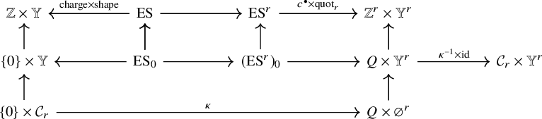
 $$ \begin{align} \begin{aligned} \mathrm{ES} &\to \mathbb{Z} \times \mathbb{Y} \\ b &\mapsto (\mathrm{charge}(b),\mathrm{shape}(b)). \end{aligned} \end{align} $$

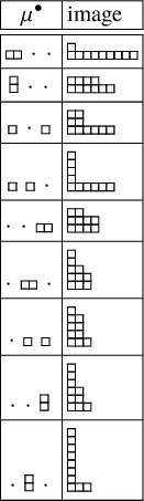
Figure 1 The shape of an edge sequence.
Example 2.1. An edge sequence b and its charge and shape are pictured in Figure 1.
2.3 Cores and quotients
Our goal is to define the bijection
 $$ \begin{align} \begin{aligned} \mathbb{Y}&\cong \mathcal{C}_r \times \mathbb{Y}^r \\ \lambda&\mapsto (\mathrm{core}_r(\lambda),\mathrm{quot}_r(\lambda)), \end{aligned} \end{align} $$
where $\mathrm {core}_r$
is the r-core and
$\mathrm {core}_r$
is the r-core and $\mathrm {quot}_r$
is the r-quotient map.
$\mathrm {quot}_r$
is the r-quotient map.
In the following diagram, all horizontal maps are bijections and vertical maps are inclusions.
Elements $b^{\bullet }=(b^0,b^1,\dotsc ,b^{r-1})\in \mathrm {ES}^r$
are called abaci. We may write them as
$b^{\bullet }=(b^0,b^1,\dotsc ,b^{r-1})\in \mathrm {ES}^r$
are called abaci. We may write them as $\{0,1,\dotsc ,r-1\}\times \mathbb {Z}$
matrices with entries in
$\{0,1,\dotsc ,r-1\}\times \mathbb {Z}$
matrices with entries in $\{0,1\}$
, where a
$\{0,1\}$
, where a $0$
is a bead and a
$0$
is a bead and a $1$
is a hole (position with no bead) and the i-th row represents the edge sequence
$1$
is a hole (position with no bead) and the i-th row represents the edge sequence $b^i$
and is the i-th runner in the abacus.
$b^i$
and is the i-th runner in the abacus.
There is a bijection $\mathrm {ES}\to \mathrm {ES}^r$
sending b to
$\mathrm {ES}\to \mathrm {ES}^r$
sending b to $(b^0,b^1,\dotsc ,b^{r-1})$
by letting
$(b^0,b^1,\dotsc ,b^{r-1})$
by letting $b^i$
select the bits in b indexed by integers congruent to i mod r:
$b^i$
select the bits in b indexed by integers congruent to i mod r: $b^i(j) = b(rj+i)$
for
$b^i(j) = b(rj+i)$
for $0\le i<r$
and
$0\le i<r$
and $j\in \mathbb {Z}$
. The inverse map is given by interleaving the sequences
$j\in \mathbb {Z}$
. The inverse map is given by interleaving the sequences $b^0,b^1,\dotsc ,b^{r-1}$
. This bijection is charge-additive:
$b^0,b^1,\dotsc ,b^{r-1}$
. This bijection is charge-additive: $\mathrm {charge}(b) = \sum _{j=0}^{r-1} \mathrm {charge}(b^j)$
. The r-fold product of the bijection (2.1) yields the bijection
$\mathrm {charge}(b) = \sum _{j=0}^{r-1} \mathrm {charge}(b^j)$
. The r-fold product of the bijection (2.1) yields the bijection $\mathrm {ES}^r \cong \mathbb {Z}^r \times \mathbb {Y}^r $
. Denote this by
$\mathrm {ES}^r \cong \mathbb {Z}^r \times \mathbb {Y}^r $
. Denote this by $b^{\bullet }=(b^0,\dotsc ,b^{r-1})\mapsto ((c_0,\dotsc ,c_{r-1}), {\lambda ^{\bullet }})$
. We write
$b^{\bullet }=(b^0,\dotsc ,b^{r-1})\mapsto ((c_0,\dotsc ,c_{r-1}), {\lambda ^{\bullet }})$
. We write ${\lambda ^{\bullet }} = \mathrm {quot}_r(b^{\bullet })$
; this is the r-quotient. Call
${\lambda ^{\bullet }} = \mathrm {quot}_r(b^{\bullet })$
; this is the r-quotient. Call $(c_0,\dotsc ,c_{r-1})=c^{\bullet }(b^{\bullet })$
the charge vector. This indicates the position on each runner where the beads end after pushing all beads to the left. This defines the bijections going across the top row of the diagram.
$(c_0,\dotsc ,c_{r-1})=c^{\bullet }(b^{\bullet })$
the charge vector. This indicates the position on each runner where the beads end after pushing all beads to the left. This defines the bijections going across the top row of the diagram.
We now restrict all these bijections. Let $\mathrm {ES}_0 = \{b\in \mathrm {ES}\mid \mathrm {charge}(b)=0\}$
and
$\mathrm {ES}_0 = \{b\in \mathrm {ES}\mid \mathrm {charge}(b)=0\}$
and $(\mathrm {ES}^r)_0 = \{b^{\bullet }\in \mathrm {ES}^r\mid \sum _{i=0}^{r-1} c_i(b^{\bullet }) =0 \}$
. Then
$(\mathrm {ES}^r)_0 = \{b^{\bullet }\in \mathrm {ES}^r\mid \sum _{i=0}^{r-1} c_i(b^{\bullet }) =0 \}$
. Then $c^{\bullet }(b^{\bullet })$
can be viewed as an element of the
$c^{\bullet }(b^{\bullet })$
can be viewed as an element of the $\mathfrak {sl}_r$
root lattice Q (and belongs to the zero lattice
$\mathfrak {sl}_r$
root lattice Q (and belongs to the zero lattice $Q=0$
when
$Q=0$
when $r=1$
). The second row of the diagram (save the last map) is given by suitable restrictions of the top row of bijections.
$r=1$
). The second row of the diagram (save the last map) is given by suitable restrictions of the top row of bijections.
An r-core is a partition $\gamma $
which does not have r as a hook length. That is,
$\gamma $
which does not have r as a hook length. That is, $h_\gamma (i,j)\ne r$
for all
$h_\gamma (i,j)\ne r$
for all $(i,j)\in \gamma $
. We denote by
$(i,j)\in \gamma $
. We denote by $\mathcal {C}_r\subset \mathbb {Y}$
the set of r-cores. Let
$\mathcal {C}_r\subset \mathbb {Y}$
the set of r-cores. Let $\gamma $
be a partition and let
$\gamma $
be a partition and let $b\in \mathrm {ES}$
be such that
$b\in \mathrm {ES}$
be such that $\mathrm {shape}(b)=\gamma $
. Then
$\mathrm {shape}(b)=\gamma $
. Then $\gamma $
has a box
$\gamma $
has a box $(i,j)\in \gamma $
with hook-length r, that is,
$(i,j)\in \gamma $
with hook-length r, that is, $h_\gamma (i,j)=r$
, if and only if there is an index k such that
$h_\gamma (i,j)=r$
, if and only if there is an index k such that $b(k)=1$
and
$b(k)=1$
and $b(k+r)=0$
. This is equivalent to
$b(k+r)=0$
. This is equivalent to $\mu ^{(k)}\ne \varnothing $
, where
$\mu ^{(k)}\ne \varnothing $
, where ${\mu ^{\bullet }}=\mathrm {quot}_r(\gamma )$
and we take superscripts mod r. This proves that
${\mu ^{\bullet }}=\mathrm {quot}_r(\gamma )$
and we take superscripts mod r. This proves that $\gamma $
is an r-core if and only if the r-quotient of
$\gamma $
is an r-core if and only if the r-quotient of $\gamma $
is empty:
$\gamma $
is empty: $\mathrm {quot}_r(\gamma )=(\varnothing ^r)$
.
$\mathrm {quot}_r(\gamma )=(\varnothing ^r)$
.
Therefore, the bijection $\{0\} \times \mathbb {Y} \cong Q\times \mathbb {Y}^r$
restricts to the bijection
$\{0\} \times \mathbb {Y} \cong Q\times \mathbb {Y}^r$
restricts to the bijection $\{0\} \times \mathcal {C}_r \cong Q \times (\varnothing ^r)$
, that is,
$\{0\} \times \mathcal {C}_r \cong Q \times (\varnothing ^r)$
, that is, $\mathcal {C}_r\cong Q$
. We call this bijection
$\mathcal {C}_r\cong Q$
. We call this bijection $\kappa $
.
$\kappa $
.
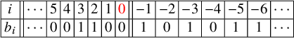
Example 2.2. Let $b\in \mathrm {ES}_0$
be as in the previous example. We have
$b\in \mathrm {ES}_0$
be as in the previous example. We have $\lambda =\mathrm {shape}(b)=(4,3,2,2)$
. Set
$\lambda =\mathrm {shape}(b)=(4,3,2,2)$
. Set $r=3$
. We map
$r=3$
. We map $b\mapsto (b^0,b^1,b^2)$
which are pictured in the matrix below. Reading up the columns of the
$b\mapsto (b^0,b^1,b^2)$
which are pictured in the matrix below. Reading up the columns of the $\{0,1,2\}\times \mathbb {Z}$
matrix, we recover b. Each runner of the abacus is an edge sequence; the corresponding shapes give the
$\{0,1,2\}\times \mathbb {Z}$
matrix, we recover b. Each runner of the abacus is an edge sequence; the corresponding shapes give the $3$
-quotient of
$3$
-quotient of $(4,3,2,2)$
, which is
$(4,3,2,2)$
, which is $(1,\varnothing ,2)$
.
$(1,\varnothing ,2)$
.
To get the $3$
-core of
$3$
-core of $\lambda $
, we move all beads to the left in each runner. This produces the second abacus. Reading up columns, we obtain the edge sequence
$\lambda $
, we move all beads to the left in each runner. This produces the second abacus. Reading up columns, we obtain the edge sequence $a=\dotsm 0001|1011\dotsm $
. Therefore,
$a=\dotsm 0001|1011\dotsm $
. Therefore, $\mathrm {core}_3(4,3,2,2)=\mathrm {shape}(a)=(2)$
. The charge sequence is
$\mathrm {core}_3(4,3,2,2)=\mathrm {shape}(a)=(2)$
. The charge sequence is $(1,-1,0)\in Q$
.
$(1,-1,0)\in Q$
.
 $$\begin{align*}\begin{array}{c||p{10pt}p{10pt}p{10pt}|p{10pt}p{10pt}p{10pt}} &2&1&0&-1&-2&-3 \\ \hline \hline b^0& 0&1& 0&1&1&1 \\ b^1& 0&0& 0&0&1&1 \\ b^2& 0&0& 1&1&0&1 \\ \hline \end{array} \end{align*}$$

Remark 2.3. Our map $\mathrm {quot}_r$
and our definition of charge are the same as in [Reference Wen19], except that we interchange the roles of black and white dots in our Maya diagrams.
$\mathrm {quot}_r$
and our definition of charge are the same as in [Reference Wen19], except that we interchange the roles of black and white dots in our Maya diagrams.
When considering a fixed r, we simply write $\mathrm {core}=\mathrm {core}_r$
and
$\mathrm {core}=\mathrm {core}_r$
and $\mathrm {quot}=\mathrm {quot}_r$
.
$\mathrm {quot}=\mathrm {quot}_r$
.
2.4 Cores and ribbons
Consider $\mu ,\lambda \in \mathbb {Y}$
such that
$\mu ,\lambda \in \mathbb {Y}$
such that $\mu \subset \lambda $
. The skew shape
$\mu \subset \lambda $
. The skew shape $\lambda /\mu :=D(\lambda )-D(\mu )$
is a
$\lambda /\mu :=D(\lambda )-D(\mu )$
is a $\mu $
-addable and
$\mu $
-addable and $\lambda $
-removable r-ribbon if
$\lambda $
-removable r-ribbon if $|\lambda |-|\mu |=r$
and the set of boxes
$|\lambda |-|\mu |=r$
and the set of boxes $\lambda /\mu $
is rookwise connected (i.e., any two boxes in
$\lambda /\mu $
is rookwise connected (i.e., any two boxes in $\lambda /\mu $
can be connected by a chain of horizontally and vertically adjacent boxes in
$\lambda /\mu $
can be connected by a chain of horizontally and vertically adjacent boxes in $\lambda /\mu $
) with at most one element on each southwest-northeast diagonal. Then an r-core is precisely a partition that has no removable r-ribbon. One way to obtain
$\lambda /\mu $
) with at most one element on each southwest-northeast diagonal. Then an r-core is precisely a partition that has no removable r-ribbon. One way to obtain $\mathrm {core}(\mu )$
is to repeatedly remove (removable) r-ribbons starting with
$\mathrm {core}(\mu )$
is to repeatedly remove (removable) r-ribbons starting with $\mu $
until an r-core is reached; by definition, this is
$\mu $
until an r-core is reached; by definition, this is $\mathrm {core}(\mu )$
. This is well defined: one obtains the same r-core independently of the order of removal of r-ribbons. It is the same as moving the beads in the abacus to the left.
$\mathrm {core}(\mu )$
. This is well defined: one obtains the same r-core independently of the order of removal of r-ribbons. It is the same as moving the beads in the abacus to the left.
2.5 Cores to root lattice
Recall that Q denotes the $\mathfrak {sl}_r$
root lattice (or
$\mathfrak {sl}_r$
root lattice (or $Q=0$
in the case
$Q=0$
in the case $r=1$
), realized as the zero sum elements in the lattice
$r=1$
), realized as the zero sum elements in the lattice $\mathbb {Z}^I$
:
$\mathbb {Z}^I$
:
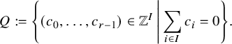 $$\begin{align*}Q:=\left\{(c_0,\ldots, c_{r-1})\in\mathbb{Z}^I\, \middle|\, \sum_{i\in I}c_i=0\right\}. \end{align*}$$
Let $\epsilon _i\in \mathbb {Z}^I$
be the i-th coordinate vector. Then Q is the spanned by the elements
$\epsilon _i\in \mathbb {Z}^I$
be the i-th coordinate vector. Then Q is the spanned by the elements
 $$\begin{align*}\alpha_i:=\epsilon_{i-1}-\epsilon_i,\qquad i\in I. \end{align*}$$
We realize the simple roots of $\mathfrak {sl}_r$
as the
$\mathfrak {sl}_r$
as the $\alpha _i$
for
$\alpha _i$
for $i\neq 0$
.
$i\neq 0$
.
Another way to compute the bijection $\kappa : \mathcal {C} \to Q$
is as follows. Define the map
$\kappa : \mathcal {C} \to Q$
is as follows. Define the map $\kappa :\mathbb {Y}\to Q$
by
$\kappa :\mathbb {Y}\to Q$
by
 $$ \begin{align*} \kappa(\mu) = -\sum_{(p,q)\in\mu} \alpha_{q-p}. \end{align*} $$
It is not difficult to show that the restriction of $\kappa $
to
$\kappa $
to $\mathcal {C}$
is the same as the bijection
$\mathcal {C}$
is the same as the bijection $\mathcal {C}\cong Q$
constructed above.
$\mathcal {C}\cong Q$
constructed above.
Example 2.4. Let $r=3$
and consider the
$r=3$
and consider the $3$
-core
$3$
-core $(2)$
. We put
$(2)$
. We put $\alpha _{q-p}$
into the box
$\alpha _{q-p}$
into the box $(p,q)$
:
$(p,q)$
:
Thus, $\kappa ((2))=-(\alpha _0+\alpha _2)=\alpha _1$
, which agrees with the charge sequence
$\kappa ((2))=-(\alpha _0+\alpha _2)=\alpha _1$
, which agrees with the charge sequence $(1,-1,0)\in Q$
computed above.
$(1,-1,0)\in Q$
computed above.
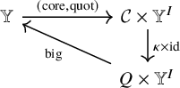
Define the bijection $\mathrm {big}:Q\times \mathbb {Y}^I\to \mathbb {Y}$
via the following commutative diagram:
$\mathrm {big}:Q\times \mathbb {Y}^I\to \mathbb {Y}$
via the following commutative diagram:
Example 2.5. We list the elements ${\mu ^{\bullet }}\in \mathbb {Y}^I$
of total size
${\mu ^{\bullet }}\in \mathbb {Y}^I$
of total size $2$
and their images under
$2$
and their images under ${\mu ^{\bullet }}\mapsto \mathrm {big}(-\alpha _1,{\mu ^{\bullet }})$
.
${\mu ^{\bullet }}\mapsto \mathrm {big}(-\alpha _1,{\mu ^{\bullet }})$
.
2.6 Symmetric functions
Let $\Lambda $
be the algebra of symmetric functions over
$\Lambda $
be the algebra of symmetric functions over $\mathbb {K}=\mathbb {Q}(q,t)$
in infinitely many variables [Reference Macdonald9, §I.2]. Denote by
$\mathbb {K}=\mathbb {Q}(q,t)$
in infinitely many variables [Reference Macdonald9, §I.2]. Denote by $\Lambda ^{I}=\Lambda ^{\otimes I}$
the I-fold tensor power of
$\Lambda ^{I}=\Lambda ^{\otimes I}$
the I-fold tensor power of $\Lambda $
over
$\Lambda $
over $\mathbb {K}$
, which is a graded
$\mathbb {K}$
, which is a graded $\mathbb {K}$
-algebra with grading given by the sum of degrees in each tensor factor. For
$\mathbb {K}$
-algebra with grading given by the sum of degrees in each tensor factor. For $f\in \Lambda $
, we write
$f\in \Lambda $
, we write $f[X^{(i)}]$
to indicate the element of
$f[X^{(i)}]$
to indicate the element of $\Lambda ^I$
with
$\Lambda ^I$
with $1$
in tensor factors
$1$
in tensor factors $j\ne i$
and f in factor i. The power sums
$j\ne i$
and f in factor i. The power sums $p_k[X^{(i)}]$
for
$p_k[X^{(i)}]$
for $i\in I$
and
$i\in I$
and $k>0$
generate
$k>0$
generate $\Lambda ^I$
as a
$\Lambda ^I$
as a $\mathbb {K}$
-algebra. We write
$\mathbb {K}$
-algebra. We write $X^{\bullet }$
for the I-tuple of alphabets
$X^{\bullet }$
for the I-tuple of alphabets $(X^{(0)},\dotsc ,X^{(r-1)})$
and often denote by
$(X^{(0)},\dotsc ,X^{(r-1)})$
and often denote by $f[X^{\bullet }]$
a generic element of
$f[X^{\bullet }]$
a generic element of $\Lambda ^I$
. Note that each alphabet
$\Lambda ^I$
. Note that each alphabet $X^{(i)}$
itself contains infinitely many variables.
$X^{(i)}$
itself contains infinitely many variables.
For an I-tuple of partitions ${\lambda ^{\bullet }}=(\lambda ^{(0)},\lambda ^{(1)},\dotsc ,\lambda ^{(r-1)})\in \mathbb {Y}^I$
, define the tensor Schur function
${\lambda ^{\bullet }}=(\lambda ^{(0)},\lambda ^{(1)},\dotsc ,\lambda ^{(r-1)})\in \mathbb {Y}^I$
, define the tensor Schur function $s_{\lambda ^{\bullet }}=\bigotimes _{i\in I} s_{\lambda ^{(i)}}=\prod _{i\in I} s_{\lambda ^{(i)}}[X^{(i)}]$
. Let
$s_{\lambda ^{\bullet }}=\bigotimes _{i\in I} s_{\lambda ^{(i)}}=\prod _{i\in I} s_{\lambda ^{(i)}}[X^{(i)}]$
. Let $\langle -,-\rangle $
be the Hall pairing on
$\langle -,-\rangle $
be the Hall pairing on $\Lambda ^I$
, which is given by
$\Lambda ^I$
, which is given by $\langle s_{\lambda ^{\bullet }}, s_{\mu ^{\bullet }} \rangle = \delta _{{\lambda ^{\bullet }},{\mu ^{\bullet }}}$
. For
$\langle s_{\lambda ^{\bullet }}, s_{\mu ^{\bullet }} \rangle = \delta _{{\lambda ^{\bullet }},{\mu ^{\bullet }}}$
. For $f\in \Lambda ^I$
, we denote by
$f\in \Lambda ^I$
, we denote by $f^{\perp }$
be the adjoint under the Hall pairing to the operator of multiplication by f. Explicitly,
$f^{\perp }$
be the adjoint under the Hall pairing to the operator of multiplication by f. Explicitly,
 $$\begin{align*}\left[p_n^{\perp}[X^{(i)}], p_m[X^{(j)}]\right]=n\delta_{n,m}\delta_{i,j}, \end{align*}$$
where we view $p_m[X^{(j)}]$
as a multiplication operator.
$p_m[X^{(j)}]$
as a multiplication operator.
For any $a\in \mathbb {K}$
, define the
$a\in \mathbb {K}$
, define the $\mathbb {K}$
-algebra automorphism
$\mathbb {K}$
-algebra automorphism $\mathcal {P}_{\mathrm {id}-a\chi ^{-1}}$
of
$\mathcal {P}_{\mathrm {id}-a\chi ^{-1}}$
of $\Lambda ^I$
by
$\Lambda ^I$
by
 $$ \begin{align} \mathcal{P}_{\mathrm{id}-a\chi^{-1}}(p_k[X^{(i)}]) = p_k[X^{(i)}]-a^{k}p_k[X^{(i-1)}] \end{align} $$
for all $i\in I$
and
$i\in I$
and $k>0$
. (The notation
$k>0$
. (The notation $\mathcal {P}_{\mathrm {id}-a\chi ^{-1}}$
arises from more general matrix plethysms
$\mathcal {P}_{\mathrm {id}-a\chi ^{-1}}$
arises from more general matrix plethysms $\mathcal {P}_A$
for
$\mathcal {P}_A$
for $A\in \mathrm {Mat}_{I\times I}(\mathbb {K})$
defined in [Reference Orr and Shimozono15].)
$A\in \mathrm {Mat}_{I\times I}(\mathbb {K})$
defined in [Reference Orr and Shimozono15].)
2.7 Wreath Macdonald functions
For a partition $\lambda $
, let
$\lambda $
, let
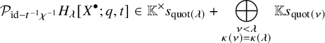
 $H_{\lambda }[X^{\bullet };q,t]$
be the wreath Macdonald functions [Reference Haiman7, Conjecture 7.2.19], as defined in [Reference Wen19, §2.3].Footnote 1 These are characterized by the conditions
$H_{\lambda }[X^{\bullet };q,t]$
be the wreath Macdonald functions [Reference Haiman7, Conjecture 7.2.19], as defined in [Reference Wen19, §2.3].Footnote 1 These are characterized by the conditions
 $$ \begin{align} \mathcal{P}_{\mathrm{id} - q \chi^{-1}} H_{\lambda} [X^{\bullet};q,t] &\in \mathbb{K}^{\times} s_{\mathrm{quot}(\lambda)} + \bigoplus_{\substack{\nu> \lambda \\ \kappa(\nu)=\kappa(\lambda)}} \mathbb{K} s_{\mathrm{quot}(\nu)} \end{align} $$
 $$ \begin{align} \mathcal{P}_{\mathrm{id}-t^{-1}\chi^{-1}}H_{\lambda}[X^{\bullet};q,t] &\in \mathbb{K}^{\times} s_{\mathrm{quot}(\lambda)} + \bigoplus_{\substack{\nu<\lambda\\ \kappa(\nu)=\kappa(\lambda)}} \mathbb{K} s_{\mathrm{quot}(\nu)} \end{align} $$
 $$ \begin{align} \langle s_{(n)}[X^{(0)}], H_{\lambda}[X^{\bullet};q,t]\rangle &= 1, \end{align} $$
where $n=|\mathrm {quot}(\lambda )|$
and
$n=|\mathrm {quot}(\lambda )|$
and $<$
is the (strict) dominance order on partitions [Reference Macdonald9, §I.1].
$<$
is the (strict) dominance order on partitions [Reference Macdonald9, §I.1].
For any $\lambda \in \mathbb {Y}$
, the wreath Macdonald P-function
$\lambda \in \mathbb {Y}$
, the wreath Macdonald P-function $P_{\lambda }[X^{\bullet };q,t^{-1}]$
is defined to be the scalar multiple of
$P_{\lambda }[X^{\bullet };q,t^{-1}]$
is defined to be the scalar multiple of $\mathcal {P}_{\mathrm {id}-t^{-1}\chi ^{-1}}(H_{\lambda }[X^{\bullet };q,t])$
in which the coefficient of
$\mathcal {P}_{\mathrm {id}-t^{-1}\chi ^{-1}}(H_{\lambda }[X^{\bullet };q,t])$
in which the coefficient of $s_{\mathrm {quot}(\lambda )}$
is
$s_{\mathrm {quot}(\lambda )}$
is $1$
. In particular,
$1$
. In particular, $P_{\lambda }[X^{\bullet };q,t^{-1}]$
satisfies the unitriangularity
$P_{\lambda }[X^{\bullet };q,t^{-1}]$
satisfies the unitriangularity
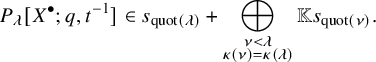 $$ \begin{align*} P_{\lambda}[X^{\bullet};q,t^{-1}]\in s_{\mathrm{quot}(\lambda)} + \bigoplus_{\substack{\nu<\lambda\\\kappa(\nu)=\kappa(\lambda)}} \mathbb{K} s_{\mathrm{quot}(\nu)}. \end{align*} $$
For any fixed $\alpha \in Q$
, the
$\alpha \in Q$
, the $P_{\lambda }[X^{\bullet };q,t^{-1}]$
such that
$P_{\lambda }[X^{\bullet };q,t^{-1}]$
such that $\kappa (\lambda )=\alpha $
form a homogeneous basis of
$\kappa (\lambda )=\alpha $
form a homogeneous basis of $\Lambda ^I$
, with
$\Lambda ^I$
, with $P_{\lambda }[X^{\bullet };q,t^{-1}]$
having degree
$P_{\lambda }[X^{\bullet };q,t^{-1}]$
having degree $|\mathrm {quot}(\lambda )|$
.
$|\mathrm {quot}(\lambda )|$
.
Our notation $P_{\lambda }[X^{\bullet };q,t^{-1}]$
agrees with the usual conventions in the classical
$P_{\lambda }[X^{\bullet };q,t^{-1}]$
agrees with the usual conventions in the classical $r=1$
case. For technical reasons, it is often convenient to work with
$r=1$
case. For technical reasons, it is often convenient to work with $P_{\lambda }[X^{\bullet };q,t^{-1}]$
rather than
$P_{\lambda }[X^{\bullet };q,t^{-1}]$
rather than $P_{\lambda }[X^{\bullet };q,t]$
, though we will eventually switch to the latter.
$P_{\lambda }[X^{\bullet };q,t]$
, though we will eventually switch to the latter.
2.8 Symmetric polynomials
For any $N_{\bullet }=(N_0,\ldots , N_{r-1})\in \left( \mathbb {Z}_{\ge 0} \right)^I$
, we can consider a finite set of variables
$N_{\bullet }=(N_0,\ldots , N_{r-1})\in \left( \mathbb {Z}_{\ge 0} \right)^I$
, we can consider a finite set of variables
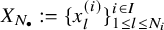 $$\begin{align*}X_{N_{\bullet}}:= \{x_{l}^{(i)}\}^{i\in I}_{1\le l\le N_i} \end{align*}$$
and the corresponding restriction map
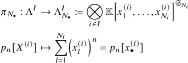 $$ \begin{align} \pi_{N_{\bullet}} : \Lambda^I &\to \Lambda^I_{N_{\bullet}}:=\bigotimes_{i\in I} \mathbb{K}\left[x_{1}^{(i)},\dotsc,x_{N_i}^{(i)}\right]^{\mathfrak{S}_{N_i}} \\ \nonumber p_n[X^{(i)}]&\mapsto \sum_{l=1}^{N_i}\left(x_{l}^{(i)}\right)^n=p_n[x_{\bullet}^{(i)}] \end{align} $$
given by the tensor product $\pi _{N_{\bullet }} = \otimes _{i\in I} \pi _{N_i}$
, where
$\pi _{N_{\bullet }} = \otimes _{i\in I} \pi _{N_i}$
, where $\pi _N : \Lambda \to \mathbb {K}[x_1,\dotsc ,x_N]^{\mathfrak {S}_N}$
is the standard projection to symmetric polynomials. We also write
$\pi _N : \Lambda \to \mathbb {K}[x_1,\dotsc ,x_N]^{\mathfrak {S}_N}$
is the standard projection to symmetric polynomials. We also write $\pi _{N_{\bullet }}(f)=f[X_{N_{\bullet }}]$
.
$\pi _{N_{\bullet }}(f)=f[X_{N_{\bullet }}]$
.
2.9 Finitization
Our main result will characterize the images $P_{\lambda }[X_{N_{\bullet }};q,t]:=\pi _{N_{\bullet }}(P_{\lambda }[X^{\bullet };q,t])$
as eigenfunctions of explicit q-difference operators. For reasons which are clarified in Remark 5.7 below, we will only consider variable number vectors
$P_{\lambda }[X_{N_{\bullet }};q,t]:=\pi _{N_{\bullet }}(P_{\lambda }[X^{\bullet };q,t])$
as eigenfunctions of explicit q-difference operators. For reasons which are clarified in Remark 5.7 below, we will only consider variable number vectors $N_{\bullet }$
for
$N_{\bullet }$
for $P_{\lambda }$
which are compatible with
$P_{\lambda }$
which are compatible with $\mathrm {core}(\lambda )$
in the following way. If
$\mathrm {core}(\lambda )$
in the following way. If $\kappa (\lambda )=\alpha =(c_0,c_1,\dotsc ,c_{r-1})$
, then we stipulate that
$\kappa (\lambda )=\alpha =(c_0,c_1,\dotsc ,c_{r-1})$
, then we stipulate that $P_{\lambda }$
will only be assigned variables
$P_{\lambda }$
will only be assigned variables $X_{N_{\bullet }}$
where
$X_{N_{\bullet }}$
where $N_{\bullet }$
is equivalent to
$N_{\bullet }$
is equivalent to $-\kappa (\lambda )$
modulo
$-\kappa (\lambda )$
modulo $\mathbb {Z}(1,\dotsc ,1)$
; that is,
$\mathbb {Z}(1,\dotsc ,1)$
; that is,
 $$ \begin{align} N_{i}-N_{i-1}=(\alpha_i^\vee,\kappa(\lambda))=(\alpha_i^\vee,\alpha)=c_{i-1}-c_{i},\quad \text{for all } i\in I, \end{align} $$
where
-
• $\alpha _i^\vee $
is the coroot for
$i\not =0$
;
$\alpha _i^\vee $
is the coroot for
$i\not =0$
; -
•
$\alpha _0=-\alpha _1-\cdots -\alpha _{r-1}$
; -
•
$(-,-):Q^\vee \times Q\to \mathbb {Z}$
is the standard pairing between
$\mathfrak {sl}_r$
root and coroot lattices.


Identifying the lattices $Q^\vee \cong Q$
and realizing Q inside
$Q^\vee \cong Q$
and realizing Q inside $\mathbb {Z}^I$
as above,
$\mathbb {Z}^I$
as above, $(-,-)$
becomes the dot product on
$(-,-)$
becomes the dot product on $\mathbb {Z}^I$
and
$\mathbb {Z}^I$
and $\alpha _i^\vee =\epsilon _{i-1}-\epsilon _i$
for all
$\alpha _i^\vee =\epsilon _{i-1}-\epsilon _i$
for all $i\in I$
.
$i\in I$
.
Example 2.6. In the setting of Example 2.2, the root lattice element is $\kappa (\lambda )=(1,-1,0)$
. The smallest variable number vector which we allow for
$\kappa (\lambda )=(1,-1,0)$
. The smallest variable number vector which we allow for $\lambda =(4,3,2,2)$
is therefore
$\lambda =(4,3,2,2)$
is therefore $N_{\bullet }=(0,2,1)$
. To this we can add the vector
$N_{\bullet }=(0,2,1)$
. To this we can add the vector $(1,1,1)$
any number of times.
$(1,1,1)$
any number of times.
Lemma 2.7. Under the compatibility condition (2.9) between $N_{\bullet }\in (\mathbb {Z}_{\ge 0})^I$
and
$N_{\bullet }\in (\mathbb {Z}_{\ge 0})^I$
and $\alpha \in Q$
, we have the following:
$\alpha \in Q$
, we have the following:
-
1. The quantity
is divisible by r.
$$\begin{align*}|N_{\bullet}|:=\sum_{i\in I}N_i\end{align*}$$
-
2. For
$\lambda \in \mathbb {Y}$
with
$\kappa (\lambda )=\alpha $
and
$\ell (\lambda )\le |N_{\bullet }|$
, where we count
$$\begin{align*}N_i=\#\left\{ 1\le b\le |N_{\bullet}| : b-\lambda_b\equiv i+1\mbox{ mod }r \right\}, \end{align*}$$
$\lambda _b=0$
if
$\ell (\lambda )<b\le |N_{\bullet }|$
; in particular,
$\mathrm {quot}(\lambda )=\lambda ^{\bullet }$
satisfies
$\ell (\lambda ^{(i)})\leq N_i$
for all
$i\in I$
.
-
3. For any
$\lambda ^{\bullet }\in \mathbb {Y}^I$
satisfying
$\ell (\lambda ^{(i)})\leq N_i$
for all i, the partition
$\lambda =\mathrm {big}(\lambda ^{\bullet },\alpha )$
satisfies
$\ell (\lambda )\le |N_{\bullet }|$
.


Proof.
-
1. This follows from the fact that
$N_{\bullet }$
and
$-\kappa (\lambda )$
are congruent modulo
$\mathbb {Z}(1,\dotsc ,1)$
, and the coordinates of the latter sum to zero. -
2. This follows from [Reference Macdonald9, I.1, Ex. 8] after taking our labeling conventions into account.
-
3. For any edge sequence b, the length of
$\mathrm {shape}(b)$
is precisely the number of
$0$
’s positioned to the right of at least one
$1$
. Given
$\alpha \in Q$
, our choice of
$N_{\bullet }$
ensures that the number of
$0$
’s positioned to the right of
$1$
’s in the interleaved edge sequence defining
$\lambda $
will not exceed
$|N_{\bullet }|$
.


An immediate consequence of parts (2) and (3) of Lemma 2.7 is the following:
Proposition 2.8. Under the compatibility condition (2.9) between $N_{\bullet }\in (\mathbb {Z}_{\ge 0})^I$
and
$N_{\bullet }\in (\mathbb {Z}_{\ge 0})^I$
and $\alpha \in Q$
, the wreath Macdonald polynomials
$\alpha \in Q$
, the wreath Macdonald polynomials $P_{\lambda }[X_{N_{\bullet }};q,t]$
indexed by
$P_{\lambda }[X_{N_{\bullet }};q,t]$
indexed by $\lambda \in \mathbb {Y}$
satisfying
$\lambda \in \mathbb {Y}$
satisfying $\ell (\lambda )\le |N_{\bullet }|$
and
$\ell (\lambda )\le |N_{\bullet }|$
and $\kappa (\lambda )=\alpha $
form a basis of
$\kappa (\lambda )=\alpha $
form a basis of $\Lambda ^I_{N_{\bullet }}$
.
$\Lambda ^I_{N_{\bullet }}$
.
3 Quantum toroidal algebra
To ensure compatibility with [Reference Wen19] and [Reference Tsymbaliuk17], we assume that $r\ge 3$
from this point on.Footnote 2
$r\ge 3$
from this point on.Footnote 2
3.1 The algebra
$U_{\mathfrak {q},\mathfrak {d}}(\ddot {\mathfrak {sl}}_r)$

Let $\mathfrak {q}$
and
$\mathfrak {q}$
and $\mathfrak {d}$
be two indeterminates, and set
$\mathfrak {d}$
be two indeterminates, and set $\mathbb {F}:=\mathbb {C}(\mathfrak {q}^{\frac {1}{2}},\mathfrak {d}^{\frac {1}{2}})$
.
$\mathbb {F}:=\mathbb {C}(\mathfrak {q}^{\frac {1}{2}},\mathfrak {d}^{\frac {1}{2}})$
.
3.1.1 Generators and relations
For $i,j\in I=\mathbb {Z}/r\mathbb {Z}$
, we set
$i,j\in I=\mathbb {Z}/r\mathbb {Z}$
, we set
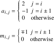 $$ \begin{align*} a_{i,j}&=\left\{\begin{array}{ll} 2 & j=i \\ -1 & j=i\pm 1 \\ 0 & \mbox{otherwise} \end{array}\right. \\[7pt] m_{i,j}&=\left\{\begin{array}{ll} \mp 1 & j=i\pm 1\\ 0 & \mbox{otherwise} \end{array}\right. \end{align*} $$
and we define
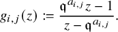 $$\begin{align*}g_{i,j}(z):=\frac{\mathfrak{q}^{a_{i,j}}z-1}{z-\mathfrak{q}^{a_{i,j}}}. \end{align*}$$
The quantum toroidal algebra $U_{s,u}(\ddot {\mathfrak {sl}}_r)$
is a unital associative
$U_{s,u}(\ddot {\mathfrak {sl}}_r)$
is a unital associative $\mathbb {F}$
-algebra with generators
$\mathbb {F}$
-algebra with generators
 $$\begin{align*}\{e_{i,k},f_{i,k},\psi_{i,k},\psi_{i,0}^{-1},\gamma^{\pm\frac{1}{2}}, \mathfrak{q}^{\pm d_1},\mathfrak{q}^{\pm d_2}\}_{i\in I}^{k\in\mathbb{Z}}. \end{align*}$$
Its relations are described in terms of currents:
 $$ \begin{align*} e_i(z) & :=\sum_{k\in\mathbb{Z}}e_{i,k}z^{-k}\\[7pt] f_i(z) & :=\sum_{k\in\mathbb{Z}}f_{i,k}z^{-k}\\[7pt] \psi_i^{\pm}(z) & :=\psi_{i,0}^{\pm 1}+\sum_{k>0}\psi_{i,\pm k}z^{\mp k}. \end{align*} $$
The relations are then
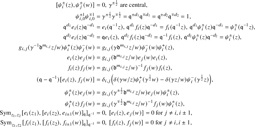 $$ \begin{align*} [\psi_i^{\pm}(z),\psi_j^{\pm}(w)]&=0,\,\gamma^{\pm\frac{1}{2}}\mbox{ are central},\\ \psi_{i,0}^{\pm1}\psi_{i,0}^{\mp1}&=\gamma^{\pm\frac{1}{2}}\gamma^{\mp\frac{1}{2}}=\mathfrak{q}^{\pm d_1}\mathfrak{q}^{\mp d_1}=\mathfrak{q}^{\pm d_2}\mathfrak{q}^{\mp d_2}=1,\\ \mathfrak{q}^{d_1}e_i(z)\mathfrak{q}^{-d_1}&=e_i(\mathfrak{q}^{-1} z),\, \mathfrak{q}^{d_1}f_i(z)\mathfrak{q}^{-d_1}=f_i(\mathfrak{q}^{-1} z),\, \mathfrak{q}^{d_1}\psi_i^{\pm}(z)\mathfrak{q}^{-d_1}=\psi_i^{\pm}(\mathfrak{q}^{-1} z),\\ \mathfrak{q}^{d_2}e_i(z)\mathfrak{q}^{-d_2}&=\mathfrak{q} e_i(z),\, \mathfrak{q}^{d_2}f_i(z)\mathfrak{q}^{-d_2}=\mathfrak{q}^{-1} f_i(z),\, \mathfrak{q}^{d_2}\psi_i^{\pm}(z)\mathfrak{q}^{-d_2}=\psi_i^{\pm}( z),\\ g_{i,j}(\gamma^{-1}\mathfrak{d}^{m_{i,j}}z/w)\psi_i^{+}(z)\psi_j^{-}(w)&=g_{i,j}(\gamma\mathfrak{d}^{m_{i,j}} z/w)\psi_j^{-}(w)\psi_i^{+}(z),\\ e_i(z)e_j(w)&=g_{i,j}(\mathfrak{d}^{m_{i,j}}z/w)e_j(w)e_i(z),\\ f_i(z)f_j(w)&=g_{i,j}(\mathfrak{d}^{m_{i,j}}z/w)^{-1}f_j(w)f_i(z),\\ (\mathfrak{q}-\mathfrak{q}^{-1})[e_i(z),f_j(w)]&=\delta_{i,j}\left(\delta(\gamma w/z)\psi_i^+(\gamma^{\frac{1}{2}}w)-\delta(\gamma z/w)\psi_i^-(\gamma^{\frac{1}{2}}z)\right),\\ \psi_i^{\pm}(z)e_j(w)&=g_{i,j}(\gamma^{\pm\frac{1}{2}}\mathfrak{d}^{m_{i,j}}z/w)e_j(w)\psi_i^{\pm}(z),\\ \psi_i^{\pm}(z)f_j(w)&=g_{i,j}(\gamma^{\mp\frac{1}{2}}\mathfrak{d}^{m_{i,j}}z/w)^{-1}f_j(w)\psi_i^{\pm}(z),\\ \mathrm{Sym}_{z_1,z_2}[e_i(z_1),[e_i(z_2),e_{i\pm1}(w)]_{\mathfrak{q}}]_{\mathfrak{q}^{-1}}&=0,\,[e_i(z),e_j(w)]=0\mbox{ for }j\not=i,i\pm1,\\ \mathrm{Sym}_{z_1,z_2}[f_i(z_1),[f_i(z_2),f_{i\pm1}(w)]_{\mathfrak{q}}]_{\mathfrak{q}^{-1}}&=0,\,[f_i(z),f_j(w)]=0\mbox{ for }j\not=i,i\pm1,\end{align*} $$
Here, $\delta (z)$
denotes the delta function
$\delta (z)$
denotes the delta function
 $$\begin{align*}\delta(z)=\sum_{k\in\mathbb{Z}}z^k\end{align*}$$
and for $v\in \mathbb {F}$
,
$v\in \mathbb {F}$
, $[a,b]_v=ab-v ba$
is the v-commutator. We will also work with elements
$[a,b]_v=ab-v ba$
is the v-commutator. We will also work with elements $\{h_{i, k}\}_{i\in I}^{k\not = 0}$
defined by
$\{h_{i, k}\}_{i\in I}^{k\not = 0}$
defined by
 $$ \begin{align} \psi_i^{\pm}(z)=\psi_{i,0}^{\pm 1}\exp\left(\pm(\mathfrak{q}-\mathfrak{q}^{-1})\sum_{k>0}h_{i,\pm k}z^{\mp k}\right). \end{align} $$
Finally, we denote by
-
•
$'\ddot {U}$
the subalgebra obtained by dropping the generator
$\mathfrak {q}^{d_1}$
; -
•
$\ddot {U}'$
the subalgebra obtained by dropping the generator
$\mathfrak {q}^{d_2}$
; -
•
$'\ddot {U}'$
the subalgebra obtained by dropping both generators
$\mathfrak {q}^{d_1}$
and
$\mathfrak {q}^{d_2}$
.


3.1.2 Miki automorphism
We recall that $U_{\mathfrak {q},\mathfrak {d}}(\ddot {\mathfrak {sl}}_r)$
contains two copies of the quantum affine algebra
$U_{\mathfrak {q},\mathfrak {d}}(\ddot {\mathfrak {sl}}_r)$
contains two copies of the quantum affine algebra $U_{\mathfrak {q}}(\dot {\mathfrak {sl}}_r)$
. The first, called the vertical copy, is generated by currents where
$U_{\mathfrak {q}}(\dot {\mathfrak {sl}}_r)$
. The first, called the vertical copy, is generated by currents where $i\not =0$
. This copy is given in the new Drinfeld presentation. However, the second copy, called the horizontal copy, is generated by the constant terms of all the currents. This copy is given in the Drinfeld-Jimbo presentation. We do not go into detail on these two subalgebras as we will not need them in the sequel. However, we mention them because they give the ‘two loops’ of the quantum toroidal algebra. Let
$i\not =0$
. This copy is given in the new Drinfeld presentation. However, the second copy, called the horizontal copy, is generated by the constant terms of all the currents. This copy is given in the Drinfeld-Jimbo presentation. We do not go into detail on these two subalgebras as we will not need them in the sequel. However, we mention them because they give the ‘two loops’ of the quantum toroidal algebra. Let $\eta $
denote the
$\eta $
denote the $\mathbb {C}(\mathfrak {q})$
-linear antiautomorphism of
$\mathbb {C}(\mathfrak {q})$
-linear antiautomorphism of $'\ddot {U}'$
defined by
$'\ddot {U}'$
defined by
 $$ \begin{align} \eta(\mathfrak{d})&=\mathfrak{d}^{-1}\nonumber\\ \eta(e_{i,k})&=e_{i,-k},\, \eta(f_{i,k})=f_{i,-k},\, \eta(h_{i,k})=-\gamma^kh_{i,-k},\\ \eta(\psi_{i,0})&=\psi_{i,0}^{-1},\,\eta(\gamma^{\frac{1}{2}})=\gamma^{\frac{1}{2}}.\nonumber \end{align} $$
The following beautiful result of Miki gives the ‘S-transformation’ of the torus:
Theorem 3.1 [Reference Miki10]
There is an algebra automorphism $\varsigma $
of
$\varsigma $
of $'\ddot {U}'$
that sends the horizontal copy of
$'\ddot {U}'$
that sends the horizontal copy of $U_{\mathfrak {q}}(\dot {\mathfrak {sl}}_r)$
to the vertical copy. Moreover,
$U_{\mathfrak {q}}(\dot {\mathfrak {sl}}_r)$
to the vertical copy. Moreover, $\varsigma $
satisfies
$\varsigma $
satisfies $\varsigma ^{-1}=\eta \varsigma \eta $
.
$\varsigma ^{-1}=\eta \varsigma \eta $
.
3.1.3 Heisenberg subalgebras
Recall the generators $\{h_{i,n}\}_{i\in I}^{n\not =0}$
defined by (3.1). Together with
$\{h_{i,n}\}_{i\in I}^{n\not =0}$
defined by (3.1). Together with $\gamma ^{\pm \frac {1}{2}}$
, these elements generate a rank r Heisenberg algebra. The relations are
$\gamma ^{\pm \frac {1}{2}}$
, these elements generate a rank r Heisenberg algebra. The relations are
 $$ \begin{align} [h_{i, n}, h_{j,n'}]=\delta_{n,-n'}\frac{(\gamma^n-\gamma^{-n})\mathfrak{d}^{-nm_{i,j}}[na_{i,j}]_{\mathfrak{q}}}{(\mathfrak{q}-\mathfrak{q}^{-1})n}\\ \gamma^{\frac{1}{2}}\mbox{ is central},\nonumber \end{align} $$
where $[n]_v$
is the usual quantum number:
$[n]_v$
is the usual quantum number:
 $$\begin{align*}[n]_v=\frac{v^n-v^{-n}}{v-v^{-1}}. \end{align*}$$
We define dual elements $\{h_{i,n}^{\perp }\}_{i\in I}^{n\not =0}$
by
$\{h_{i,n}^{\perp }\}_{i\in I}^{n\not =0}$
by
 $$ \begin{align} \begin{aligned} h_{i,n}^{\perp}&= \frac{\mathfrak{q}^{n}(\mathfrak{q}-\mathfrak{q}^{-1})n}{(1-\mathfrak{q}^{nr}\mathfrak{d}^{nr})(1-\mathfrak{q}^{nr}\mathfrak{d}^{-nr})[n]_{\mathfrak{q}}} \sum_{j,k=0}^{r-1} \mathfrak{q}^{n(j+k)}\mathfrak{d}^{n(j-k)}h_{i+j-k, n}\\ h_{i,-n}^{\perp}&= \frac{\mathfrak{q}^{n}(\mathfrak{q}-\mathfrak{q}^{-1})n}{(1-\mathfrak{q}^{nr}\mathfrak{d}^{nr})(1-\mathfrak{q}^{nr}\mathfrak{d}^{-nr})[n]_{\mathfrak{q}}} \sum_{j,k=0}^{r-1} \mathfrak{q}^{n(j+k)}\mathfrak{d}^{n(j-k)}h_{i-j+k,-n}. \end{aligned} \end{align} $$
Lemma 3.2. The elements $\{h_{i,n}^{\perp }\}$
are characterized by
$\{h_{i,n}^{\perp }\}$
are characterized by
 $$ \begin{align} [h_{i,n}^{\perp}, h_{j,-n'}]=[h_{j,n'}, h_{i,-n}^{\perp}]=\delta_{i,j}\delta_{n,n'}(\gamma^n-\gamma^{-n}) \end{align} $$
for $k>0$
.
$k>0$
.
Proof. Equations (3.5) obviously characterizes these elements. For $n>0$
, let
$n>0$
, let $M_n$
be the matrix
$M_n$
be the matrix $r\times r$
matrix
$r\times r$
matrix
 $$\begin{align*}\left(M_n\right)_{ij}=\mathfrak{d}^{-nm_{i,j}}[na_{i,j}]_{\mathfrak{q}}. \end{align*}$$
We view the rows and coloumns as indexed by I. Equation (3.3) can be rephrased as
 $$\begin{align*}[h_{i,n}, h_{j,-n}]= \left(M_{n}\right)_{ij}\frac{(\gamma^n-\gamma^{-n})}{(\mathfrak{q}-\mathfrak{q}^{-1})n}. \end{align*}$$
For any $r\times r$
matrix A (with rows and columns indexed by I), set
$r\times r$
matrix A (with rows and columns indexed by I), set
 $$ \begin{align*} Ah_{i,n}=\sum_{k\in I} A_{ki}h_{k,n},\qquad\qquad\qquad Ah_{i,-n}=\sum_{k\in I}A_{ki}h_{k,-n}. \end{align*} $$
We then have for $n>0$
,
$n>0$
,
 $$ \begin{align*} \left[Ah_{i,n}, h_{j,-n}\right]&=(A^TM_n)_{ij}\frac{(\gamma^n-\gamma^{-n})}{(\mathfrak{q}-\mathfrak{q}^{-1})n},& \left[h_{j,n}, Ah_{i,-n}\right]&=\left(M_nA\right)_{ji}\frac{(\gamma^n-\gamma^{-n})}{(\mathfrak{q}-\mathfrak{q}^{-1})n}. \end{align*} $$
Thus, to obtain (3.5), we need to invert $M_n$
. To that end, we factorize
$M_n$
. To that end, we factorize $M_n$
:
$M_n$
:
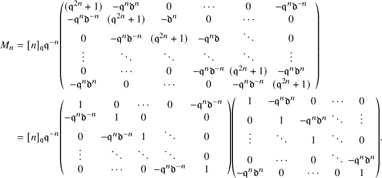 $$ \begin{align*} M_n&=[n]_{\mathfrak{q}}\mathfrak{q}^{-n} \begin{pmatrix} (\mathfrak{q}^{2n}+1) & -\mathfrak{q}^n\mathfrak{d}^n & 0&\cdots & 0 & -\mathfrak{q}^n\mathfrak{d}^{-n}\\ -\mathfrak{q}^n\mathfrak{d}^{-n} & (\mathfrak{q}^{2n}+1) & -\mathfrak{d}^n & 0 &\cdots & 0\\ 0 & -\mathfrak{q}^n\mathfrak{d}^{-n} & (\mathfrak{q}^{2n}+1) & -\mathfrak{q}^n\mathfrak{d}&\ddots &0\\ \vdots & \ddots& \ddots& \ddots& \ddots & \vdots&\\ 0 & \cdots & 0 & -\mathfrak{q}^n\mathfrak{d}^{-n} & (\mathfrak{q}^{2n}+1) &-\mathfrak{q}^n\mathfrak{d}^n\\ -\mathfrak{q}^n\mathfrak{d}^n & 0 &\cdots & 0& -\mathfrak{q}^n\mathfrak{d}^{-n} & (\mathfrak{q}^{2n}+1) \end{pmatrix}\\ &=[n]_{\mathfrak{q}}\mathfrak{q}^{-n} \begin{pmatrix} 1 & 0&\cdots & 0 & -\mathfrak{q}^n\mathfrak{d}^{-n}\\ -\mathfrak{q}^n\mathfrak{d}^{-n} & 1 & 0 & & 0\\ 0 & -\mathfrak{q}^{n}\mathfrak{d}^{-n} & 1 & \ddots &0\\ \vdots & \ddots& \ddots& \ddots& 0&\\ 0 & \cdots & 0 & -\mathfrak{q}^{n}\mathfrak{d}^{-n} & 1 \\ \end{pmatrix} \begin{pmatrix} 1 & -\mathfrak{q}^n\mathfrak{d}^n & 0&\cdots & 0 \\ 0 & 1 & -\mathfrak{q}^n\mathfrak{d}^n & \ddots & \vdots\\ \vdots & \ddots & 1 & \ddots &0\\ 0 & \cdots & 0 & \ddots &-\mathfrak{q}^{n}\mathfrak{d}^n\\ -\mathfrak{q}^{n}\mathfrak{d}^n & 0 &\cdots & 0& 1 \end{pmatrix}. \end{align*} $$
Inverting the last two matrices, we obtain (3.4).
We denote by $\ddot {U}^0$
the subalgebra generated by
$\ddot {U}^0$
the subalgebra generated by $\{\gamma ^{\pm \frac {1}{2}}\}\cup \{h_{i, k}\}_{i\in I}^{k\not = 0}$
an call it the vertical Heisenberg subalgebra. In analogy with 3.1.2, we call
$\{\gamma ^{\pm \frac {1}{2}}\}\cup \{h_{i, k}\}_{i\in I}^{k\not = 0}$
an call it the vertical Heisenberg subalgebra. In analogy with 3.1.2, we call $\varsigma (\ddot {U}^0)$
the horizontal Heisenberg subalgebra.
$\varsigma (\ddot {U}^0)$
the horizontal Heisenberg subalgebra.
Remark 3.3. In [Reference Wen19], the author defines elements $\{b_{i,k}^{\perp }\}$
in terms of a pairing that is not used in this paper. By comparing the commutator (3.3) to the pairing in loc. cit., we have that
$\{b_{i,k}^{\perp }\}$
in terms of a pairing that is not used in this paper. By comparing the commutator (3.3) to the pairing in loc. cit., we have that
 $$\begin{align*}h_{i,k}^{\perp}=-b_{i,k}^{\perp}. \end{align*}$$
3.2 Vertex representation $U_{\mathfrak {q},\mathfrak {d}}(\ddot {\mathfrak {sl}}_r)$
directly interacts with the wreath Macdonald polynomials via its vertex representation, originally constructed by Yoshihisa Saito [Reference Saito16].
$U_{\mathfrak {q},\mathfrak {d}}(\ddot {\mathfrak {sl}}_r)$
directly interacts with the wreath Macdonald polynomials via its vertex representation, originally constructed by Yoshihisa Saito [Reference Saito16].
3.2.1 Twisted group algebra
Recall that Q and $Q^\vee $
denote the
$Q^\vee $
denote the $\mathfrak {sl}_r$
root and coroot lattices, respectively, with simple roots
$\mathfrak {sl}_r$
root and coroot lattices, respectively, with simple roots $\{\alpha _j\}_{j=1}^{r-1}$
, simple coroots
$\{\alpha _j\}_{j=1}^{r-1}$
, simple coroots $\{\alpha ^\vee _j\}_{j=1}^{r-1}$
, and canonical pairing
$\{\alpha ^\vee _j\}_{j=1}^{r-1}$
, and canonical pairing $(-,-) : Q^\vee \times Q \to \mathbb {Z}$
:
$(-,-) : Q^\vee \times Q \to \mathbb {Z}$
:
 $$\begin{align*}(\alpha_i^\vee,\alpha_j)=a_{i,j}. \end{align*}$$
Let P denote the $\mathfrak {sl}_r$
weight lattice and
$\mathfrak {sl}_r$
weight lattice and $\{\Lambda _p\}_{j=1}^{r-1}$
the fundamental weights. We will also need
$\{\Lambda _p\}_{j=1}^{r-1}$
the fundamental weights. We will also need
 $$\begin{align*}\alpha_0=-\sum_{j=1}^{r-1}\alpha_j,\quad \alpha^\vee_0=-\sum_{j=1}^{r-1}\alpha^\vee_j,\quad \Lambda_0:=0. \end{align*}$$
We have that $\{\alpha _2,\ldots ,\alpha _{r-1},\Lambda _{r-1}\}$
is a basis of P.
$\{\alpha _2,\ldots ,\alpha _{r-1},\Lambda _{r-1}\}$
is a basis of P.
The twisted group algebra $\mathbb {F}\{P\}$
is the
$\mathbb {F}\{P\}$
is the $\mathbb {F}$
-algebra generated by
$\mathbb {F}$
-algebra generated by $\{e^{\alpha _j}\}_{j=2}^{r-1}\cup \{e^{\Lambda _{r-1}}\}$
satisfying the relations
$\{e^{\alpha _j}\}_{j=2}^{r-1}\cup \{e^{\Lambda _{r-1}}\}$
satisfying the relations
 $$ \begin{align*} e^{\alpha_i}e^{\alpha_j}&=(-1)^{\left( \alpha^\vee_i,\alpha_j\right)}e^{\alpha_j}e^{\alpha_i}\\ e^{\alpha_i}e^{\Lambda_{r-1}}&=(-1)^{\delta_{i,r-1}}e^{\Lambda_{r-1}}e^{\alpha_i}. \end{align*} $$
Given a general $\alpha \in P$
, we write
$\alpha \in P$
, we write $\alpha =\sum _{j=2}^{r-1}m_j\alpha _j+m_{r}\Lambda _{r-1}$
and then set
$\alpha =\sum _{j=2}^{r-1}m_j\alpha _j+m_{r}\Lambda _{r-1}$
and then set
 $$\begin{align*}e^{\alpha}=e^{m_2\alpha_2}\cdots e^{m_{r-1}\alpha_{r-1}}e^{m_r\Lambda_{r-1}}.\end{align*}$$
For example,
 $$ \begin{align} \begin{aligned} e^{\alpha_1}&=e^{-2\alpha_2}e^{-3\alpha_3}\cdots e^{-(r-1)\alpha_{r-1}}e^{r\Lambda_{r-1}}\\ e^{\alpha_0}&=e^{\alpha_2}e^{2\alpha_3}\cdots e^{(r-2)\alpha_{r-1}}e^{-r\Lambda_{r-1}}. \end{aligned} \end{align} $$
Define $\mathbb {F}\{Q\}$
to be the subalgebra of
$\mathbb {F}\{Q\}$
to be the subalgebra of $\mathbb {F}\{P\}$
generated by
$\mathbb {F}\{P\}$
generated by $\{e^{\alpha _i}\}_{i=1}^{r-1}$
.
$\{e^{\alpha _i}\}_{i=1}^{r-1}$
.
3.2.2 Vertex operators
The vertical Heisenberg subalgebra $\ddot {U}^0$
has a Fock representation
$\ddot {U}^0$
has a Fock representation $F_r$
defined as follows. Let
$F_r$
defined as follows. Let $\ddot {U}^0_+$
denote the subalgebra generated by
$\ddot {U}^0_+$
denote the subalgebra generated by $\gamma ^{\frac {1}{2}}$
and
$\gamma ^{\frac {1}{2}}$
and $\{h_{i,k}\}_{i\in I}^{k>0}$
.
$\{h_{i,k}\}_{i\in I}^{k>0}$
. $\ddot {U}^0_+$
has a one-dimensional representation
$\ddot {U}^0_+$
has a one-dimensional representation $\mathbb {F}_{\mathfrak {q}}$
where
$\mathbb {F}_{\mathfrak {q}}$
where $\gamma ^{\frac {1}{2}}$
acts by
$\gamma ^{\frac {1}{2}}$
acts by $\mathfrak {q}^{\frac {1}{2}}$
while
$\mathfrak {q}^{\frac {1}{2}}$
while $h_{i,k}$
acts by
$h_{i,k}$
acts by $0$
.
$0$
. $F_r$
is then the induced representation
$F_r$
is then the induced representation
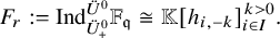 $$\begin{align*}F_r:=\mathrm{Ind}_{\ddot{U}^0_+}^{\ddot{U}^0}\mathbb{F}_{\mathfrak{q}}\cong\mathbb{K}[h_{i,-k}]_{i\in I}^{k>0}. \end{align*}$$
The vertex representation is defined on the space $W:=F_r\otimes \mathbb {F}\{Q\}$
. For
$W:=F_r\otimes \mathbb {F}\{Q\}$
. For $v\otimes e^\alpha \in W$
where
$v\otimes e^\alpha \in W$
where
 $$ \begin{align*} v&=h_{i_1,-k_1}\cdots h_{i_N,-k_N} v_0\\ \alpha&=\sum_{j=1}^{r-1}m_j\alpha_j, \end{align*} $$
we define the operators $h_{i,k}$
,
$h_{i,k}$
, $e^\beta $
,
$e^\beta $
, $\partial _{\alpha _i}$
,
$\partial _{\alpha _i}$
, $z^{H_{i,0}}$
and d by
$z^{H_{i,0}}$
and d by
 $$ \begin{align} \nonumber h_{i,k}(v\otimes e^\alpha )&:=(h_{i,k}v)\otimes e^\alpha ,\, e^\beta(v\otimes e^\alpha ):=v\otimes(e^\beta e^\alpha ),\\ \nonumber \partial_{\alpha_i}(v\otimes e^\alpha )&:=\left( \alpha^\vee_i,\alpha\right) v\otimes e^\alpha ,\\ z^{H_{i,0}}(v\otimes e^\alpha )&:=z^{\left( \alpha^\vee_i,\alpha\right)} \mathfrak{d}^{\frac{1}{2}\sum_{j=1}^{r-1}\left( \alpha^\vee_i,m_j\alpha_j\right) m_{i,j}}v\otimes e^\alpha ,\\ \nonumber d(v\otimes e^\alpha )&:=-\left(\dfrac{(\alpha,\alpha)}{2}+\sum_{i=1}^N k_i\right)v\otimes e^\alpha. \end{align} $$
Theorem 3.4 [Reference Saito16]
Let $\vec {c}=(c_0,\ldots , c_{r-1})\in (\mathbb {F}^{\times })^r$
. The following formulas endow W with an action of
$\vec {c}=(c_0,\ldots , c_{r-1})\in (\mathbb {F}^{\times })^r$
. The following formulas endow W with an action of $\ddot {U}'$
:
$\ddot {U}'$
:
 $$ \begin{align*} \rho_{\vec{c}}(e_i(z))&=c_i\exp\left(\sum_{k>0}\frac{\mathfrak{q}^{-\frac{k}{2}}}{[k]_{\mathfrak{q}}}h_{i,-k}z^k\right)\\ &\times\exp\left(-\sum_{k>0}\frac{\mathfrak{q}^{-\frac{k}{2}}}{[k]_{\mathfrak{q}}}h_{i,k}z^{-k}\right)e^{\alpha_i} z^{1+H_{i,0}},\\ \rho_{\vec{c}}(f_i(z))&=\frac{(-1)^{r\delta_{i,0}}}{c_i}\exp\left(-\sum_{k>0}\frac{\mathfrak{q}^{\frac{k}{2}}}{[k]_{\mathfrak{q}}}h_{i,-k}z^k\right)\\ &\times\exp\left(\sum_{k>0}\frac{\mathfrak{q}^{\frac{k}{2}}}{[k]_{\mathfrak{q}}}h_{i,k}z^{-k}\right)e^{-\alpha_i} z^{1-H_{i,0}},\\\rho_{\vec{c}}(\psi_i^{\pm}(z))&=\exp\left(\pm(\mathfrak{q}-\mathfrak{q}^{-1})\sum_{k>0}h_{i,\pm k}z^{\mp k}\right)\mathfrak{q}^{\pm\partial_{\alpha_i}},\\ &\rho_{\vec{c}}(\gamma^{\frac{1}{2}})=\mathfrak{q}^{\frac{1}{2}},\,\rho_{\vec{c}}(\mathfrak{q}^{d_1})=\mathfrak{q}^{d}. \end{align*} $$
3.2.3 Embedding symmetric functions
We can let $\Lambda ^{I}$
act on
$\Lambda ^{I}$
act on $F_r$
via multiplication operators given by
$F_r$
via multiplication operators given by
 $$ \begin{align} p_k[X^{(i)}]\mapsto \frac{k}{[k]_{\mathfrak{q}}}h_{i,-k} \end{align} $$
for $k>0$
. To obtain an identification
$k>0$
. To obtain an identification $W\cong \Lambda ^{I}\otimes \mathbb {F}\left\{ Q \right\}$
, we need to embed
$W\cong \Lambda ^{I}\otimes \mathbb {F}\left\{ Q \right\}$
, we need to embed $\mathbb {K}$
into
$\mathbb {K}$
into $\mathbb {F}$
:
$\mathbb {F}$
:
 $$ \begin{align} q=\mathfrak{q}\mathfrak{d},\, t=\mathfrak{q}\mathfrak{d}^{-1}. \end{align} $$
Applying $\rho _{\vec {c}}$
to (3.5) sends
$\rho _{\vec {c}}$
to (3.5) sends $\gamma \mapsto \mathfrak {q}$
. Thus, as operators on
$\gamma \mapsto \mathfrak {q}$
. Thus, as operators on $\Lambda ^{I}$
, we have the identification
$\Lambda ^{I}$
, we have the identification
 $$\begin{align*}p_k[X^{(i)}]^{\perp}\mapsto kh_{i,k}^{\perp}. \end{align*}$$
Now consider transforming the formulas for $\rho _{\vec {c}}$
using matrix plethysms on
$\rho _{\vec {c}}$
using matrix plethysms on $\{p_k[X^{(i)}]\}$
. We can obtain an isomorphic representation as long as we perform a corresponding transformation on
$\{p_k[X^{(i)}]\}$
. We can obtain an isomorphic representation as long as we perform a corresponding transformation on $\{h_{i,k}\}$
to maintain the commutation relations, using (3.3) as a guide. First, we define
$\{h_{i,k}\}$
to maintain the commutation relations, using (3.3) as a guide. First, we define $\rho _{\vec {c}}^+$
by performing the plethysm
$\rho _{\vec {c}}^+$
by performing the plethysm
 $$\begin{align*}p_k[X^{(i)}]\mapsto \mathfrak{q}^{\frac{k}{2}}\left(p_k[X^{(i)}]-t^{-k}p_k[X^{(i-1)}]\right). \end{align*}$$
For $\rho _{\vec {c}}^+$
, we will only be interested in the currents
$\rho _{\vec {c}}^+$
, we will only be interested in the currents $\{e_i(z)\}$
, although we have a representation for the entire algebra:
$\{e_i(z)\}$
, although we have a representation for the entire algebra:
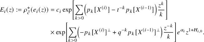 $$ \begin{align} \begin{aligned} E_i(z):=\rho_{\vec{c}}^+(e_i(z))&=c_i\exp\left[\sum_{k>0}\left(p_{k}[X^{(i)}]-t^{-k}p_{k}[X^{(i-1)}]\right)\frac{z^k}{k}\right]\\ &\times\exp\left[\sum_{k>0}\left(-p_{k}[X^{(i)}]^{\perp}+q^{-k}p_k[X^{(i-1)}]^{\perp}\right)\frac{z^{-k}}{k}\right]e^{\alpha_i} z^{1+H_{i,0}}. \end{aligned} \end{align} $$
Similarly, we define $\rho _{c}^-$
by performing the plethysm
$\rho _{c}^-$
by performing the plethysm
 $$\begin{align*}p_k[X^{(i)}]\mapsto \mathfrak{q}^{-\frac{k}{2}}\left(t^{k}p_k[X^{(i)}]-p_k[X^{(i-1)}]\right). \end{align*}$$
Here, we will only be interested in the action of the currents $\{ f_i(z)\}$
:
$\{ f_i(z)\}$
:
 $$ \begin{align} \begin{aligned} F_i(z):=\rho_{\vec{c}}^-(f_i(z))&= \frac{(-1)^{r\delta_{i,0}}}{c_i}\exp\left[\sum_{k>0}\left(-t^{k}p_{k}[X^{(i)}]+p_{k}[X^{(i-1)}]\right)\frac{z^k}{k}\right]\\ &\times\exp\left[\sum_{k>0}\left(q^{k}p_{k}[X^{(i)}]^{\perp}-p_{k}[X^{(i-1)}]^{\perp}\right)\frac{z^{-k}}{k}\right]e^{-\alpha_i} z^{1-H_{i,0}}. \end{aligned} \end{align} $$
The following is a consequence of the main result of [Reference Wen19]:
Theorem 3.5. Under both representations $\rho _{\vec {c}}^{\pm }$
,
$\rho _{\vec {c}}^{\pm }$
, $\varsigma (\ddot {U}^0)$
acts diagonally on
$\varsigma (\ddot {U}^0)$
acts diagonally on $\{P_{\lambda }[ X^{\bullet } ;q,t^{-1} ]\otimes e^{\kappa (\lambda )}\}$
.
$\{P_{\lambda }[ X^{\bullet } ;q,t^{-1} ]\otimes e^{\kappa (\lambda )}\}$
.
Remark 3.6. The paper [Reference Wen19] is concerned with the transformed wreath Macdonald functions $\{H_{\lambda }[X^{\bullet } ;q,t]\}$
. The plethysms used to define
$\{H_{\lambda }[X^{\bullet } ;q,t]\}$
. The plethysms used to define $\rho _{\vec {c}}^{\pm }$
are both scalar multiples of the plethysm
$\rho _{\vec {c}}^{\pm }$
are both scalar multiples of the plethysm $\mathcal {P}_{\mathrm {id}-t^{-1}\chi ^{-1}}$
which sends
$\mathcal {P}_{\mathrm {id}-t^{-1}\chi ^{-1}}$
which sends $H_{\lambda }[X^{\bullet }; q,t]$
to a scalar multiple of
$H_{\lambda }[X^{\bullet }; q,t]$
to a scalar multiple of $P_{\lambda }[ X^{\bullet };q,t^{-1} ]$
.
$P_{\lambda }[ X^{\bullet };q,t^{-1} ]$
.
3.2.4 Normal ordering
Later, we will make use of a particular expression for products of the currents $\{E_i(z)\}$
and
$\{E_i(z)\}$
and $\{F_i(z)\}$
. We will need notation for an ordered product or composition of noncommuting operators
$\{F_i(z)\}$
. We will need notation for an ordered product or composition of noncommuting operators $a_1,\ldots , a_m$
:
$a_1,\ldots , a_m$
:
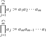 $$ \begin{align} \begin{aligned} \overset{\curvearrowright}{\prod_{j=1}^m}a_j&:=a_1 a_2\cdots a_m\\ \overset{\curvearrowleft}{\prod_{j=1}^m}a_j&:=a_m a_{m-1}\cdots a_1 \end{aligned} \end{align} $$
Proposition 3.7. For $p\in I$
, we have
$p\in I$
, we have
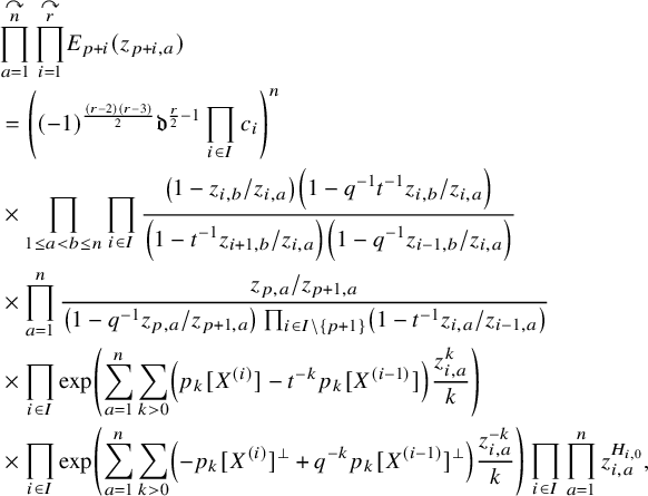 $$ \begin{align} \begin{aligned} &\overset{\curvearrowright}{\prod_{a=1}^n}\,\overset{\curvearrowright}{\prod_{i=1}^{r}}E_{p+i}(z_{p+i,a})\\ &= \left( (-1)^{\frac{(r-2)(r-3)}{2}}\mathfrak{d}^{\frac{r}{2}-1}\prod_{i\in I} c_i\right)^n\\ &\times\prod_{1\le a<b\le n}\prod_{i\in I} \frac{\displaystyle\left(1-z_{i,b}/z_{i,a}\right)\left(1-q^{-1}t^{-1}z_{i,b}/z_{i,a}\right)}{\displaystyle\left(1-t^{-1}z_{i+1,b}/z_{i,a}\right)\left(1-q^{-1}z_{i-1,b}/z_{i,a}\right)}\\ &\times\prod_{a=1}^n \frac{z_{p,a}/z_{p+1,a}} {\left(1-q^{-1}z_{p,a}/z_{p+1,a}\right) \prod_{i\in I\setminus\{p+1\}} \left(1-t^{-1}z_{i,a}/z_{i-1,a}\right)}\\ &\times\prod_{i\in I}\exp\left(\sum_{a=1}^n\sum_{k>0}\left(p_{k}[X^{(i)}]-t^{-k}p_k[X^{(i-1)}]\right)\frac{z_{i,a}^{k}}{k}\right)\\ &\times\prod_{i\in I}\exp\left(\sum_{a=1}^n\sum_{k>0}\left(-p_{k}[X^{(i)}]^{\perp}+q^{-k}p_k[X^{(i-1)}]^{\perp}\right)\frac{z_{i,a}^{-k}}{k}\right) \prod_{i\in I}\prod_{a=1}^n z_{i,a}^{H_{i,0}}, \end{aligned} \end{align} $$
where all rational functions are Laurent series expanded assuming
 $$ \begin{align} |z_{i,a}|=1,\,|q|>1,\,|t|>1. \end{align} $$
For the F-currents, we have
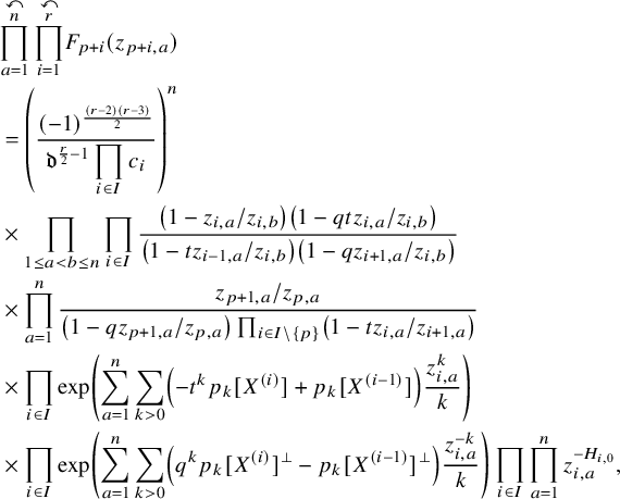 $$ \begin{align} &\overset{\curvearrowleft}{\prod_{a=1}^n}\,\overset{\curvearrowleft}{\prod_{i=1}^{r}}F_{p+i}(z_{p+i,a})\nonumber\\ &=\left( \frac{(-1)^{\frac{(r-2)(r-3)}{2}}}{\displaystyle\mathfrak{d}^{\frac{r}{2}-1} \prod_{i\in I} c_i}\right)^n\nonumber\\ &\times\prod_{1\le a<b\le n}\prod_{i\in I} \frac{\left(1-z_{i,a}/z_{i,b}\right)\left(1-qtz_{i,a}/z_{i,b}\right)}{\left(1-tz_{i-1,a}/z_{i,b}\right)\left(1-qz_{i+1,a}/z_{i,b}\right)}\\&\times \prod_{a=1}^n\frac{z_{p+1,a}/z_{p,a}}{\left(1-qz_{p+1,a}/z_{p,a}\right) \prod_{i\in I\setminus\{p\}} \left(1-tz_{i,a}/z_{i+1,a}\right)}\nonumber\\ &\times\prod_{i\in I}\exp\left(\sum_{a=1}^n\sum_{k>0}\left(-t^{k}p_{k}[X^{(i)}]+p_k[X^{(i-1)}]\right)\frac{z_{i,a}^{k}}{k}\right)\nonumber\\ &\times\prod_{i\in I}\exp\left(\sum_{a=1}^n\sum_{k>0}\left(q^{k}p_{k}[X^{(i)}]^{\perp}-p_k[X^{(i-1)}]^{\perp}\right)\frac{z_{i,a}^{-k}}{k}\right) \prod_{i\in I}\prod_{a=1}^n z_{i,a}^{-H_{i,0}},\nonumber \end{align} $$
where all rational functions are Laurent series expanded assuming
 $$ \begin{align} |z_{i,a}|=1,\, |q|< 1,\, |t|<1. \end{align} $$
Proof. The computation is standard. We will only go over the signs and powers of $\mathfrak {d}$
. The sign comes from the commutation of
$\mathfrak {d}$
. The sign comes from the commutation of $\{e^{\alpha _i}\}$
; in both cases, these factors simplify to
$\{e^{\alpha _i}\}$
; in both cases, these factors simplify to $\pm e^0$
. For the E-currents, if
$\pm e^0$
. For the E-currents, if $p=0$
, then by (3.6),
$p=0$
, then by (3.6),
 $$\begin{align*}e^{\alpha_1}= e^{r\Lambda_{r-1}}e^{-(r-1)\alpha_{r-1}}\cdots e^{-3\alpha_3}e^{-2\alpha_2}.\end{align*}$$
Thus,
 $$\begin{align*}e^{\alpha_1}e^{\alpha_2}\cdots e^{\alpha_{r-1}}=(-1)^{\frac{(r-2)(r-3)}{2}}e^{r\Lambda_{r-1}}e^{-(r-2)\alpha_{r-1}}\cdots e^{-2\alpha_3}e^{-\alpha_2}. \end{align*}$$
However, if $p\not =0$
, we have
$p\not =0$
, we have
 $$ \begin{align*} e^{\alpha_0}e^{\alpha_1}&= (-1)^{\frac{(r-1)(r-2)}{2}-1}e^{-\alpha_2}\cdots e^{-\alpha_{r-1}}\\ &=(-1)^{\frac{(r-1)(r-2)}{2}+r-3}e^{-\alpha_{r-1}}\cdots e^{-\alpha_{2}}\\ &= (-1)^{\frac{(r-2)(r-3)}{2}}e^{-\alpha_{r-1}}\cdots e^{-\alpha_{2}}, \end{align*} $$
which also leads to a sign of $(-1)^{\frac {(r-2)(r-3)}{2}}$
. For the F-currents, first consider the case
$(-1)^{\frac {(r-2)(r-3)}{2}}$
. For the F-currents, first consider the case $p=0$
.
$p=0$
.
 $$ \begin{align*} e^{-\alpha_0}e^{-\alpha_{r-1}}\cdots e^{-\alpha_3}e^{-\alpha_2}&= (-1)^{r+\frac{(r-2)(r-3)}{2}}e^{-2\alpha_2}e^{-3\alpha_3}\cdots e^{-(r-1)\alpha_{-r-1}}e^{r\Lambda_{r-1}}\\ &= (-1)^{r+\frac{(r-2)(r-3)}{2}}e^{r\Lambda_{r-1}}e^{-(r-1)\alpha_{r-1}}\cdots e^{-3\alpha_2}e^{-2\alpha_2}. \end{align*} $$
If $p\not =0$
, then we use that
$p\not =0$
, then we use that
 $$ \begin{align*} e^{-\alpha_1}e^{-\alpha_0}&=(-1)^re^{-\alpha_1}e^{r\Lambda_{r-1}}e^{-(r-2)\alpha_{r-1}}\cdots e^{-2\alpha_3}e^{-\alpha_2}\\ &= (-1)^{r+\frac{(r-2)(r-3)}{2}}e^{\alpha_2}e^{\alpha_3}\cdots e^{\alpha_{r-1}}. \end{align*} $$
Finally, note that $F_0(z)$
also has a sign of
$F_0(z)$
also has a sign of $(-1)^{r}$
. The power of
$(-1)^{r}$
. The power of $\mathfrak {d}$
comes from the interaction between
$\mathfrak {d}$
comes from the interaction between $\{z^{\pm H_{i,0}}\}$
and
$\{z^{\pm H_{i,0}}\}$
and $\{e^{\pm \alpha _{j}}\}$
. First observe that when considering
$\{e^{\pm \alpha _{j}}\}$
. First observe that when considering $E_i(z_{i,a})$
and
$E_i(z_{i,a})$
and $E_{j}(z_{j,b})$
for
$E_{j}(z_{j,b})$
for $a\not =b$
, the powers of
$a\not =b$
, the powers of $\mathfrak {d}$
from
$\mathfrak {d}$
from $j=i-1$
and
$j=i-1$
and $j=i+1$
cancel out. When
$j=i+1$
cancel out. When $a=b$
, there is a total power of
$a=b$
, there is a total power of $\mathfrak {d}^{\frac {r}{2}-1}$
. The case for
$\mathfrak {d}^{\frac {r}{2}-1}$
. The case for $\{F_i(z)\}$
is similar but inverted.
$\{F_i(z)\}$
is similar but inverted.
3.3 Fock representation
While our main focus will be on the vertex representation, we will consider another representation of $U_{\mathfrak {q},\mathfrak {d}}(\ddot {\mathfrak {sl}}_r)$
, called the Fock representation. Our goal will be gain some knowledge on the eigenvalues implicit in the statement of Theorem 3.5.
$U_{\mathfrak {q},\mathfrak {d}}(\ddot {\mathfrak {sl}}_r)$
, called the Fock representation. Our goal will be gain some knowledge on the eigenvalues implicit in the statement of Theorem 3.5.
3.3.1 Definition
In order to define the Fock representation, we will need some notation for partitions. For a partition $\lambda $
, let
$\lambda $
, let $\square =(a,b)\in D(\lambda )$
. We set the following:
$\square =(a,b)\in D(\lambda )$
. We set the following:
-
1.
$\chi _\square =q^{a}t^{b}$
, the character of the box; -
2.
$c_\square = b-a$
modulo r (its color); -
3.
$d_i(\lambda )$
the number of elements of
$D(\lambda )$
with content equivalent to i modulo r; -
4.
$A_i(\lambda )$
and
$R_i(\lambda )$
the addable and removable i-nodes of
$\lambda $
, respectively.


Finally, we will abbreviate $a\equiv b\mbox { mod }r$
by simply
$a\equiv b\mbox { mod }r$
by simply $a\equiv b$
and use the Kronecker delta function
$a\equiv b$
and use the Kronecker delta function $\delta _{a= b}:=\delta _{a-b,0}$
.
$\delta _{a= b}:=\delta _{a-b,0}$
.
Let $v\in \mathbb {F}^{\times }$
. The Fock representation
$v\in \mathbb {F}^{\times }$
. The Fock representation $\mathcal {F}(v)$
has a basis
$\mathcal {F}(v)$
has a basis $\{|\lambda \rangle \}$
indexed by partitions.
$\{|\lambda \rangle \}$
indexed by partitions.
Theorem 3.8 [Reference Feigin, Jimbo, Miwa and Mukhin5], cf. [Reference Wen19]
We can define a $'\ddot {U}$
-action
$'\ddot {U}$
-action $\tau _v$
on
$\tau _v$
on $\mathcal {F}(v)$
where the only nonzero matrix elements of the generators are
$\mathcal {F}(v)$
where the only nonzero matrix elements of the generators are
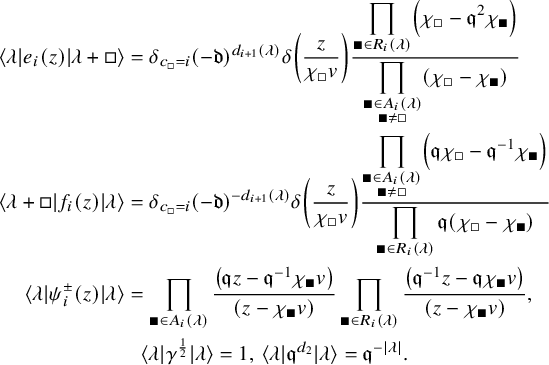 $$ \begin{gather*} \begin{aligned} \langle\lambda | e_i(z)|\lambda+\square\rangle&=\delta_{c_\square=i}(-\mathfrak{d})^{d_{i+1}(\lambda)}\delta\left( \frac{ z}{\chi_\square v}\right) \frac{\displaystyle\prod_{\blacksquare\in R_{i}(\lambda)}\left( \chi_\square-\mathfrak{q}^2\chi_\blacksquare \right)} {\displaystyle\prod_{\substack{\blacksquare\in A_{i}(\lambda)\\\blacksquare\not=\square}}\left(\chi_\square-\chi_\blacksquare\right)}\\ \langle\lambda+\square |f_i(z)|\lambda\rangle&=\delta_{c_\square=i}(-\mathfrak{d})^{-d_{i+1}(\lambda)}\delta\left(\frac{ z}{\chi_\square v}\right) \frac{\displaystyle\prod_{\substack{\blacksquare\in A_{i}(\lambda)\\\blacksquare\not=\square}}\left( \mathfrak{q}\chi_\square-\mathfrak{q}^{-1}\chi_\blacksquare \right)} {\displaystyle\prod_{\blacksquare\in R_{i}(\lambda)}\mathfrak{q}\left( \chi_\square-\chi_\blacksquare \right)}\\ \langle\lambda|\psi_i^{\pm}(z)|\lambda\rangle&= \prod_{\blacksquare\in A_{i}(\lambda)}\frac{\left(\mathfrak{q} z-\mathfrak{q}^{-1}\chi_{\blacksquare}v\right)}{\left( z-\chi_\blacksquare v\right)} \prod_{\blacksquare\in R_{i}(\lambda)}\frac{\left(\mathfrak{q}^{-1} z-\mathfrak{q}\chi_\blacksquare v\right)}{\left( z-\chi_\blacksquare v\right)}, \end{aligned}\\ \langle\lambda|\gamma^{\frac{1}{2}}|\lambda\rangle=1,\,\langle\lambda|\mathfrak{q}^{d_2}|\lambda\rangle=\mathfrak{q}^{-|\lambda|}. \end{gather*} $$
3.3.2 Tsymbaliuk isomorphism
The representation $\tau _v$
on
$\tau _v$
on $\mathcal {F}(v)$
has a cyclic vector
$\mathcal {F}(v)$
has a cyclic vector $|\varnothing \rangle $
. However,
$|\varnothing \rangle $
. However, $\rho _{\vec {c}}$
and
$\rho _{\vec {c}}$
and $\rho _{\vec {c}}^{\pm }$
also have the natural cyclic vector
$\rho _{\vec {c}}^{\pm }$
also have the natural cyclic vector $1\otimes 1\in F_r\otimes \mathbb {F}\{Q\}$
. The following theorem was proved by Tsymbaliuk:
$1\otimes 1\in F_r\otimes \mathbb {F}\{Q\}$
. The following theorem was proved by Tsymbaliuk:
Theorem 3.9 [Reference Tsymbaliuk17]
Let
 $$ \begin{align} v=(-1)^{\frac{(\ell-2)(\ell-3)}{2}}\frac{\mathfrak{q}\mathfrak{d}^{-\frac{\ell}{2}}}{c_0\cdots c_{\ell-1}}. \end{align} $$
The map of cyclic vectors
 $$\begin{align*}\mathcal{F}(v)\ni|\varnothing\rangle\mapsto 1\otimes 1\in W \end{align*}$$
induces an isomorphism between the $'\ddot {U}'$
-module
$'\ddot {U}'$
-module $\tau _v$
and the
$\tau _v$
and the $\varsigma $
-twisted modules
$\varsigma $
-twisted modules $\rho _{\vec {c}}\circ \varsigma $
,
$\rho _{\vec {c}}\circ \varsigma $
, $\rho _{\vec {c}}^{\pm }\circ \varsigma $
.
$\rho _{\vec {c}}^{\pm }\circ \varsigma $
.
The Tsymbaliuk isomorphism is defined only in terms of cyclic vectors. In light of Remark 3.6, the following result from [Reference Wen19] provides more detail on the Tsymbaliuk isomorphisms:
Theorem 3.10. The Tsymbaliuk isomorphisms (Theorem 3.9) between $\tau _v$
and
$\tau _v$
and $\rho _{\vec {c}}^{\pm }$
send
$\rho _{\vec {c}}^{\pm }$
send
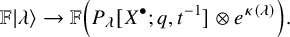 $$\begin{align*}\mathbb{F}|\lambda\rangle\to\mathbb{F} \left(P_{\lambda}[X^{\bullet};q,t^{-1}]\otimes e^{\kappa(\lambda)}\right).\end{align*}$$
Thus, we can study the eigenvalues of $\varsigma (\ddot {U}^0)$
on
$\varsigma (\ddot {U}^0)$
on $P_{\lambda }$
by instead studying the eigenvalues of
$P_{\lambda }$
by instead studying the eigenvalues of $\ddot {U}^0$
on the basis
$\ddot {U}^0$
on the basis $\{|\lambda \rangle \}$
.
$\{|\lambda \rangle \}$
.
3.3.3 Infinite-variable eigenvalues
From the formulas in Theorem 3.8, we can see that
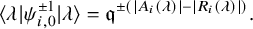 $$\begin{align*}\langle\lambda|\psi_{i,0}^{\pm 1}|\lambda\rangle= \mathfrak{q}^{\pm\left(|A_{i}(\lambda)|-|R_{i}(\lambda)|\right)}. \end{align*}$$
Therefore,
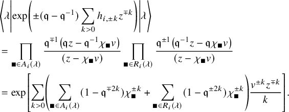 $$ \begin{align*} &\left\langle\lambda\left|\exp\left(\pm(\mathfrak{q}-\mathfrak{q}^{-1})\sum_{k>0}h_{i,\pm k}z^{\mp k}\right)\right|\lambda\right\rangle\\ &=\prod_{\blacksquare\in A_{i}(\lambda)}\frac{\mathfrak{q}^{\mp 1}\left(\mathfrak{q} z-\mathfrak{q}^{-1}\chi_{\blacksquare}v\right)}{\left( z-\chi_\blacksquare v\right)} \prod_{\blacksquare\in R_{i}(\lambda)}\frac{\mathfrak{q}^{\pm 1}\left(\mathfrak{q}^{-1} z-\mathfrak{q}\chi_\blacksquare v\right)}{\left( z-\chi_\blacksquare v\right)}\\ &= \exp\left[ \sum_{k>0}\left( \sum_{\blacksquare\in A_{i}(\lambda)}(1-\mathfrak{q}^{\mp 2k})\chi_{\blacksquare}^{\pm k} +\sum_{\blacksquare\in R_{i}(\lambda)}(1-\mathfrak{q}^{\pm 2k})\chi_\blacksquare^{\pm k}\right)\frac{v^{\pm k}z^{\mp k}}{k} \right]. \end{align*} $$
Taking logarithms, we see that for $k>0$
,
$k>0$
,
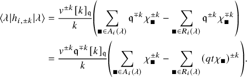 $$ \begin{align} \begin{aligned} \langle\lambda|h_{i,\pm k}|\lambda\rangle &= \frac{v^{\pm k}[ k]_{\mathfrak{q}}}{k}\left( \sum_{\blacksquare\in A_{i}(\lambda)}\mathfrak{q}^{\mp k}\chi_\blacksquare^{\pm k} -\sum_{\blacksquare\in R_{i}(\lambda)}\mathfrak{q}^{\pm k}\chi_\blacksquare^{\mp k}\right)\\ &= \frac{v^{\pm k}\mathfrak{q}^{\mp k}[ k]_{\mathfrak{q}}}{k}\left( \sum_{\blacksquare\in A_{i}(\lambda)}\chi_\blacksquare^{\pm k} - \sum_{\blacksquare\in R_{i}(\lambda)}(qt\chi_\blacksquare)^{\pm k}\right). \end{aligned} \end{align} $$
Using (3.18), we can try to piece together elements of $\ddot {U}^0$
whose eigenvalues are elementary symmetric functions in
$\ddot {U}^0$
whose eigenvalues are elementary symmetric functions in $\{q^{\pm \lambda _b}t^{\pm b}\}$
.
$\{q^{\pm \lambda _b}t^{\pm b}\}$
.
For $k\in \mathbb {Z}_{>0}$
and
$k\in \mathbb {Z}_{>0}$
and $p\in I$
, let us define
$p\in I$
, let us define
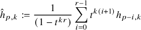 $$ \begin{align} \hat{h}_{p,k}&:=\frac{1}{(1-t^{kr})}\sum_{i=0}^{r-1}t^{ k(i+1)}h_{p-i, k} \end{align} $$
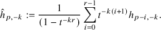 $$ \begin{align}\hspace{11.5pt} \hat{h}_{p,-k}&:= \frac{1}{(1-t^{- kr})}\sum_{i=0}^{r-1}t^{- k(i+1)}h_{p-i,- k}. \end{align} $$
Lemma 3.11. Assume $|t^{\pm 1}|<1$
(where ‘
$|t^{\pm 1}|<1$
(where ‘ $+$
’ and ‘
$+$
’ and ‘ $-$
’ are separate cases). For
$-$
’ are separate cases). For $p\in I$
, we have
$p\in I$
, we have
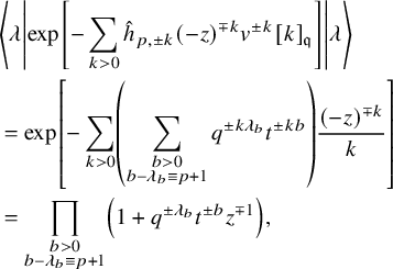 $$ \begin{align} \begin{aligned} &\left\langle\lambda\left|\exp\left[-\sum_{k>0}\hat{h}_{p,\pm k} (-z)^{\mp k}{v^{\pm k}[ k]_{\mathfrak{q}}} \right]\right|\lambda\right\rangle\\ &= \exp\left[-\sum_{k>0}\left(\sum_{\substack{b>0\\b-\lambda_b\equiv p+1 }}q^{\pm k\lambda_b}t^{\pm kb}\right)\frac{(-z)^{\mp k}}{k}\right]\\ &= \prod_{\substack{b>0\\b-\lambda_b\equiv p+1 }}\left(1+q^{\pm\lambda_b}t^{\pm b}z^{\mp 1}\right), \end{aligned} \end{align} $$
where we set $\lambda _b=0$
for all
$\lambda _b=0$
for all $b>\ell (\lambda )$
.
$b>\ell (\lambda )$
.
Proof. Comparing (3.21) to (3.18), we need to establish the equality
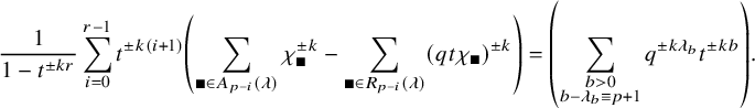 $$ \begin{align} \frac{1}{1-t^{\pm kr}}\sum_{i=0}^{r-1}t^{\pm k(i+1)}\left( \sum_{\blacksquare\in A_{p-i}(\lambda)}\chi_\blacksquare^{\pm k} - \sum_{\blacksquare\in R_{p-i}(\lambda)}(qt\chi_\blacksquare)^{\pm k}\right) =\left(\sum_{\substack{b>0\\b-\lambda_b\equiv p+1 }}q^{\pm k\lambda_b}t^{\pm kb}\right). \end{align} $$
We note that here, we consider $(1-t^{\pm kr})^{-1}$
as a geometric series. The summands on the right-hand side of (3.22) are
$(1-t^{\pm kr})^{-1}$
as a geometric series. The summands on the right-hand side of (3.22) are $qt$
-shifts of the characters of color
$qt$
-shifts of the characters of color $p+1$
boxes that are the rightmost boxes in their row. We can account for these coordinates by starting at each addable box of
$p+1$
boxes that are the rightmost boxes in their row. We can account for these coordinates by starting at each addable box of $D(\lambda )$
, going straight up until we reach a box of color
$D(\lambda )$
, going straight up until we reach a box of color $p+1$
, then moving upwards by intervals of r, and ending the search once we are above the
$p+1$
, then moving upwards by intervals of r, and ending the search once we are above the $qt$
-shift of the removable box above it. This is exactly what the left-hand side of (3.22) does. We illustrate this with Figure 2.
$qt$
-shift of the removable box above it. This is exactly what the left-hand side of (3.22) does. We illustrate this with Figure 2.
4 Shuffle algebra
We will obtain difference operators by computing the action of $\varsigma (\ddot {U}^0)$
on the vertex representation. However, computing the images of elements under
$\varsigma (\ddot {U}^0)$
on the vertex representation. However, computing the images of elements under $\varsigma $
is difficult. The shuffle algebra provides another avatar of the quantum toroidal algebra with which we can access the horizontal Heisenberg subalgebra.
$\varsigma $
is difficult. The shuffle algebra provides another avatar of the quantum toroidal algebra with which we can access the horizontal Heisenberg subalgebra.
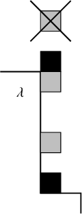
Figure 2 Illustration of the proof of Lemma 3.21. The t-shifts on the addable black box at the bottom results in the gray boxes. The latter are evenly spaced of interval r and have the desired color. The black box at the top is $qt$
times a removable box, and subtracting its t-shifts cancels out the extraneous gray boxes.
$qt$
times a removable box, and subtracting its t-shifts cancels out the extraneous gray boxes.
4.1 Definition and structures
Let $k_{\bullet }=(k_0,\ldots , k_{r-1})\in \left( \mathbb {Z}_{\ge 0} \right)^I$
and consider the function spaces:
$k_{\bullet }=(k_0,\ldots , k_{r-1})\in \left( \mathbb {Z}_{\ge 0} \right)^I$
and consider the function spaces:
 $$ \begin{align*} \mathbb{S}_{k_{\bullet}}&:=\mathbb{F}(z_{i,a})_{i\in I}^{1\le a\le k_i}\\ \mathbb{S}&:=\bigoplus_{k_{\bullet}\in\left(\mathbb{Z}_{\ge0}\right)^I}\mathbb{S}_{\vec{k}}. \end{align*} $$
The product of symmetric groups
 $$\begin{align*}\mathfrak{S}_{k_{\bullet}}:=\mathfrak{S}_{k_0}\times\cdots\times\mathfrak{S}_{k_{r-1}} \end{align*}$$
acts on $\mathbb {S}_{k_{\bullet }}$
, where the factor
$\mathbb {S}_{k_{\bullet }}$
, where the factor $\mathfrak {S}_{k_i}$
only permutes the variables
$\mathfrak {S}_{k_i}$
only permutes the variables $\{z_{i,a}\}_{a=1}^{k_i}$
. We call i the color of
$\{z_{i,a}\}_{a=1}^{k_i}$
. We call i the color of $z_{i,r}$
, so
$z_{i,r}$
, so $\mathfrak {S}_{k_{\bullet }}$
acts by color-preserving permutations. Finally, let
$\mathfrak {S}_{k_{\bullet }}$
acts by color-preserving permutations. Finally, let
 $$ \begin{align*} \mathbf{S}_{k_{\bullet}}&:=\left(\mathbb{S}_{k_{\bullet}}\right)^{\mathfrak{S}_{k_{\bullet}}}\\ \mathbf{S}&:=\bigoplus_{k_{\bullet}\in\left( \mathbb{Z}_{\ge 0} \right)^I}\mathbf{S}_{k_{\bullet}}. \end{align*} $$
Unless we say otherwise, an element of $\mathbb {S}$
with
$\mathbb {S}$
with $k_i$
variables of color i for all i is assumed to be in
$k_i$
variables of color i for all i is assumed to be in $\mathbb {S}_{k_{\bullet }}$
.
$\mathbb {S}_{k_{\bullet }}$
.
4.1.1 Shuffle product
We endow $\mathbf {S}$
with the shuffle product
$\mathbf {S}$
with the shuffle product $\star $
, defined as follows. For
$\star $
, defined as follows. For $i,j\in I$
, we define the mixing terms:
$i,j\in I$
, we define the mixing terms:
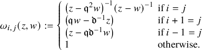 $$\begin{align*}\omega_{i,j}(z,w):=\left\{\begin{array}{ll} \left(z-\mathfrak{q}^{2}w\right)^{-1}\left(z-w\right)^{-1} & \mbox{if }i=j\\ \left(\mathfrak{q} w-\mathfrak{d}^{-1}z\right) &\mbox{if }i+1=j\\ \left(z-\mathfrak{q}\mathfrak{d}^{-1} w\right) &\mbox{if }i-1=j\\ 1 &\mbox{otherwise.} \end{array}\right.\end{align*}$$
For $F\in \mathbf {S}_{k_{\bullet }}$
and
$F\in \mathbf {S}_{k_{\bullet }}$
and $G\in \mathbf {S}_{l_{\bullet }}$
, let
$G\in \mathbf {S}_{l_{\bullet }}$
, let $F\star G\in \mathbf {S}_{k_{\bullet }+l_{\bullet }}$
be defined by
$F\star G\in \mathbf {S}_{k_{\bullet }+l_{\bullet }}$
be defined by
 $$\begin{align*}F\star G:=\frac{1}{k_{\bullet}!l_{\bullet}!}\mathrm{Sym}_{k_{\bullet}+l_{\bullet}}\left[ F\left( \left\{ z_{i,a} \right\}_{i\in I}^{1\le a\le k_i} \right)G\left( \left\{ z_{j, b} \right\}_{j\in I}^{k_j<b\le k_j+l_j} \right) \prod_{i,j\in I}\prod_{\substack{1\le a\le k_i\\k_j<b\le k_j+l_j}}\omega_{i,j}(z_{i,a},z_{j,b}) \right], \end{align*}$$
where for $n_{\bullet }\in \left( \mathbb {Z}_{\ge 0} \right)^I$
,
$n_{\bullet }\in \left( \mathbb {Z}_{\ge 0} \right)^I$
,
 $$\begin{align*}n_{\bullet}!=\prod_{i\in I}n_i!=|\mathfrak{S}_{n_{\bullet}}| \end{align*}$$
and $\mathrm {Sym}_{n_{\bullet }}$
denotes the color symmetrization (i.e., the symmetrization over
$\mathrm {Sym}_{n_{\bullet }}$
denotes the color symmetrization (i.e., the symmetrization over $\mathfrak {S}_{n_{\bullet }}$
).
$\mathfrak {S}_{n_{\bullet }}$
).
4.1.2 The shuffle algebra
Consider now for each $k_{\bullet }$
the subspace
$k_{\bullet }$
the subspace $\mathcal {S}_{k_{\bullet }}\subset \mathbf {S}_{k_{\bullet }}$
consisting of functions F satisfying the following two conditions:
$\mathcal {S}_{k_{\bullet }}\subset \mathbf {S}_{k_{\bullet }}$
consisting of functions F satisfying the following two conditions:
-
1. Pole conditions: F is of the form
(4.1)for a color-symmetric Laurent polynomial f.
$$ \begin{align} F=\frac{f(\{z_{i,r}\})}{\displaystyle \prod_{i\in I}\,\prod_{\substack{1\le r, r'\le k_i\\r\not= r'}}(z_{i,r}-\mathfrak{q}^2z_{i,r'})} \end{align} $$
-
2. Wheel conditions: F has a well-defined finite limit when
for any choice of i,
$$\begin{align*}\frac{z_{i,r_1}}{z_{i+\epsilon,s}}\rightarrow\mathfrak{q}\mathfrak{d}^\epsilon\mbox{ and }\frac{z_{i+\epsilon,s}}{z_{i,r_2}}\rightarrow\mathfrak{q}\mathfrak{d}^{-\epsilon}\end{align*}$$
$r_1$
,
$r_2$
, s and
$\epsilon $
, where
$\epsilon \in \{\pm 1\}$
. This is equivalent to specifying that the Laurent polynomial f in the pole conditions evaluates to zero at
$$ \begin{align*} \begin{aligned} z_{i,r_1}&=\mathfrak{q}\mathfrak{d}^{\epsilon}z_{i+\epsilon,s},& z_{i+\epsilon,s}&=\mathfrak{q}\mathfrak{d}^{-\epsilon}z_{i,r_2}. \end{aligned} \end{align*} $$


We set
 $$\begin{align*}\mathcal{S}:=\bigoplus_{k_{\bullet}\in\left( \mathbb{Z}_{\ge 0} \right)^I}\mathcal{S}_{k_{\bullet}}. \end{align*}$$
The following is standard:
Proposition 4.1 [Reference Neguţ11, Proposition 3.3]
The shuffle product $\star $
defines an associative product on
$\star $
defines an associative product on $\mathbf {S}$
and
$\mathbf {S}$
and $\mathcal {S}$
is closed under
$\mathcal {S}$
is closed under $\star $
.
$\star $
.
We call $(\mathcal {S},\star )$
the shuffle algebra of type
$(\mathcal {S},\star )$
the shuffle algebra of type $\hat {A}_{r-1}$
.
$\hat {A}_{r-1}$
.
4.1.3 Relation to
$U_{\mathfrak {q},\mathfrak {d}}(\ddot {\mathfrak {sl}_r})$

Let
-
•
$\ddot {U}^+\subset U_{\mathfrak {q},\mathfrak {d}}(\ddot {\mathfrak {sl}_r})$
be the subalgebra generated by
$\left\{ e_{i}(z) \right\}_{i\in I}$
and -
•
$\ddot {U}^-\subset U_{\mathfrak {q},\mathfrak {d}}(\ddot {\mathfrak {sl}_r})$
be the subalgebra generated by
$\left\{ f_{i}(z) \right\}_{i\in I}$
.


Correspondingly, we set $\mathcal {S}^+:=\mathcal {S}$
and
$\mathcal {S}^+:=\mathcal {S}$
and $\mathcal {S}^-:=\mathcal {S}^{op}$
. The following key structural result was proved by Neguţ:
$\mathcal {S}^-:=\mathcal {S}^{op}$
. The following key structural result was proved by Neguţ:
Theorem 4.2 [Reference Neguţ11] $\mathcal {S}^{\pm }$
is generated by
$\mathcal {S}^{\pm }$
is generated by $\{z_{i,1}^n\}_{i\in I}^{n\in \mathbb {Z}}$
and
$\{z_{i,1}^n\}_{i\in I}^{n\in \mathbb {Z}}$
and
 $$ \begin{align*} \Psi_+(z_{i,1}^n)&= e_{i,n}\\ \Psi_-(z_{i,1}^n)&= f_{i,n} \end{align*} $$
induce algebra isomorphisms $\Psi _{\pm }:\mathcal {S}^{\pm }\rightarrow \ddot {U}^{\pm }$
.
$\Psi _{\pm }:\mathcal {S}^{\pm }\rightarrow \ddot {U}^{\pm }$
.
Finally, note that the subalgebras $\ddot {U}^{\pm }$
are each closed under
$\ddot {U}^{\pm }$
are each closed under $\eta $
. We will need to understand how the antiautomorphism
$\eta $
. We will need to understand how the antiautomorphism $\eta $
is manifested on the shuffle side:
$\eta $
is manifested on the shuffle side:
Proposition 4.3. For $F\in \mathcal {S}^{\pm }_{k_{\bullet }}$
, define
$F\in \mathcal {S}^{\pm }_{k_{\bullet }}$
, define
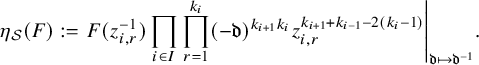 $$\begin{align*}\eta_{\mathcal{S}}(F):= \left.F(z_{i,r}^{-1})\prod_{i\in I}\prod_{r=1}^{k_i}(-\mathfrak{d})^{k_{i+1}k_i} z_{i,r}^{k_{i+1}+k_{i-1}-2(k_i-1)}\right|_{\mathfrak{d}\mapsto\mathfrak{d}^{-1}}. \end{align*}$$
We have
 $$ \begin{align} \Psi_+^{-1}\eta\Psi_+(F)=\Psi_-^{-1}\eta\Psi_-(F)=\eta_{\mathcal{S}}(F). \end{align} $$
Proof. Equation (4.2) is true when $F=z_{i,1}^n$
is a generator. To see that it is a
$F=z_{i,1}^n$
is a generator. To see that it is a $\mathbb {C}(\mathfrak {q})$
-linear algebra antiautomorphism that inverts
$\mathbb {C}(\mathfrak {q})$
-linear algebra antiautomorphism that inverts $\mathfrak {d}$
, we first observe that
$\mathfrak {d}$
, we first observe that
 $$ \begin{align} \begin{aligned} z^{-2}w^{-2}\omega_{i,i}(z^{-1},w^{-1})\bigg|_{\mathfrak{d}\mapsto\mathfrak{d}^{-1}}&=\omega_{i,i}(w,z)\\ zw(-\mathfrak{d})\omega_{i,i+1}(z^{-1},w^{-1})\bigg|_{\mathfrak{d}\mapsto\mathfrak{d}^{-1}}&=\omega_{i+1,i}(w,z)\\ zw(-\mathfrak{d})\omega_{i+1,i}(z^{-1}, w^{-1})\bigg|_{\mathfrak{d}\mapsto\mathfrak{d}^{-1}}&=\omega_{i,i+1}(w,z). \end{aligned} \end{align} $$
Now, for $F\in \mathcal {S}_{k_{\bullet }}^+$
and
$F\in \mathcal {S}_{k_{\bullet }}^+$
and $G\in \mathcal {S}_{l_{\bullet }}^+$
,
$G\in \mathcal {S}_{l_{\bullet }}^+$
,
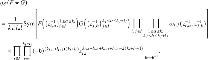 $$ \begin{align} \nonumber &\eta_{\mathcal{S}}(F\star G)\\ \nonumber &=\frac{1}{k_{\bullet}!l_{\bullet}!}\mathrm{Sym}\left[F\left(\{z_{i,a}^{-1}\}_{i\in I}^{1\le a\le k_i}\right) G\left(\{z_{j,b}^{-1}\}_{j\in I}^{k_j<b\le k_j+l_j}\right) \prod_{i,j\in I}\prod_{\substack{1\le a\le k_i\\k_j<b\le k_j+l_j}}\omega_{i,j}(z_{i,a}^{-1},z_{j,b}^{-1})\right]\\ &\quad\times \prod_{i\in I}\prod_{r=1}^{k_i+l_i}(-\mathfrak{d})^{(k_{i+1}+l_{i+1})(k_i+l_i)} z_{i,r}^{k_{i+1}+l_{i+1}+k_{i-1}+l_{i-1}-2(k_i+l_i-1)}\bigg|_{\mathfrak{d}\mapsto\mathfrak{d}^{-1}}. \end{align} $$
The monomial in (4.4) is color-symmetric, so we can move it inside the symmetrization. We can break up the exponents appearing in (4.4) as follows:
 $$ \begin{align} (k_{i+1}+l_{i+1})(k_i+l_i)&=k_{i+1}k_{i}+l_{i+1}l_i+\left[k_{i+1}l_i+k_il_{i+1}\right] \end{align} $$
 $$ \begin{align} k_{i+1}+l_{i+1}+k_{i-1}+l_{i-1}-2(k_i+l_i-1)&=k_{i+1}+k_{i-1}-2(k_i-1)+[l_{i+1}+l_{i-1}-2l_i] \end{align} $$
 $$ \begin{align} &=l_{i+1}+l_{i-1}-2(l_i-1)+[k_{i+1}+k_{i-1}-2k_i]. \end{align} $$
In (4.5), we will assign the bracketed summand to the mixing terms, $k_{i+1}k_{i}$
to F, and
$k_{i+1}k_{i}$
to F, and $l_{i+1}l_i$
to G. In a given summand of the symmetrization, if
$l_{i+1}l_i$
to G. In a given summand of the symmetrization, if $z_{i,r}$
is assigned to F, then in (4.6), we assign the bracketed summand to the mixing terms and the rest to F. However, if
$z_{i,r}$
is assigned to F, then in (4.6), we assign the bracketed summand to the mixing terms and the rest to F. However, if $z_{i,r}$
is assigned to G, then in (4.7), we assign the bracketed summand to the mixing terms and the rest to G. Then, applying (4.3), we do indeed obtain
$z_{i,r}$
is assigned to G, then in (4.7), we assign the bracketed summand to the mixing terms and the rest to G. Then, applying (4.3), we do indeed obtain
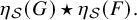 $$\begin{align*}\eta_{\mathcal{S}}(G)\star\eta_{\mathcal{S}}(F). \end{align*}$$
The case where $F,G\in \mathcal {S}^-$
is similar.
$F,G\in \mathcal {S}^-$
is similar.
4.1.4 Shuffle presentation of horizontal Heisenberg elements
Recall the vertical Heisenberg elements (3.21) whose actions on $\mathcal {F}(v)$
are related to infinite-variable Macdonald operators. Previous work [Reference Wen19] gives us a better understanding of the action of
$\mathcal {F}(v)$
are related to infinite-variable Macdonald operators. Previous work [Reference Wen19] gives us a better understanding of the action of $\varsigma ^{-1}$
on such elements. However, we need
$\varsigma ^{-1}$
on such elements. However, we need $\varsigma $
instead, and thus, we will apply the identity
$\varsigma $
instead, and thus, we will apply the identity $\varsigma =\eta \varsigma ^{-1}\eta $
(cf. Theorem 3.1) and Proposition 4.3. To that end, recall the elements
$\varsigma =\eta \varsigma ^{-1}\eta $
(cf. Theorem 3.1) and Proposition 4.3. To that end, recall the elements $\{\hat {h}_{p,\pm k}\}$
from (3.19) and (3.20). Observe that
$\{\hat {h}_{p,\pm k}\}$
from (3.19) and (3.20). Observe that
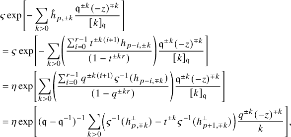 $$ \begin{align} \begin{aligned} &\varsigma\exp\left[-\sum_{k>0}\hat{h}_{p,\pm k}\frac{\mathfrak{q}^{\pm k} (-z)^{\mp k}}{[ k]_{\mathfrak{q}}} \right] \\ &=\varsigma\exp\left[-\sum_{k>0}\left(\frac{\sum_{i=0}^{r-1}t^{\pm k(i+1)}h_{p-i,\pm k}}{(1-t^{\pm kr})}\right)\frac{\mathfrak{q}^{\pm k} (-z)^{\mp k}}{[ k]_{\mathfrak{q}}} \right] \\ &=\eta\exp\left[\sum_{k>0}\left(\frac{\sum_{i=0}^{r-1}q^{\pm k(i+1)}\varsigma^{-1}(h_{p-i,\mp k})}{(1-q^{\pm kr})}\right)\frac{\mathfrak{q}^{\pm k} (-z)^{\mp k}}{[ k]_{\mathfrak{q}}} \right]\\ &= \eta\exp\left[(\mathfrak{q}-\mathfrak{q}^{-1})^{-1}\sum_{k>0}\left(\varsigma^{-1}(h_{p,\mp k}^{\perp})-t^{\pm k}\varsigma^{-1}(h_{p+1,\mp k}^{\perp})\right)\frac{q^{\pm k} (-z)^{\mp k}}{k} \right], \end{aligned} \end{align} $$
where in the last line, we use (3.3). Let $\delta =(1,\ldots , 1)\in \left( \mathbb {Z}_{\ge 0} \right)^I$
be the diagonal vector and consider the elements
$\delta =(1,\ldots , 1)\in \left( \mathbb {Z}_{\ge 0} \right)^I$
be the diagonal vector and consider the elements $\mathcal {E}_{p,n}^{\pm }\in \mathcal {S}^{\pm }$
given by
$\mathcal {E}_{p,n}^{\pm }\in \mathcal {S}^{\pm }$
given by
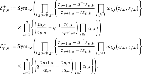 $$ \begin{align} \begin{aligned} \mathcal{E}_{p,n}^+&:= \mathrm{Sym}_{n\delta}\left( \prod_{1\le a<b\le n}\left\{\frac{z_{p+1,a}-q^{-1}z_{p,b}}{z_{p+1,a}-tz_{p,b}}\prod_{i,j\in I}\omega_{i,j}\left( z_{i,a},z_{j,b} \right)\right\}\right.\\ &\ \quad\times \left.\prod_{a=1}^n\left\{\left( \frac{z_{0,a}}{z_{p,a}}-q^{-1}\frac{z_{0,a}}{z_{p+1,a}} \right)\prod_{i\in I}z_{i,a} \right\} \right)\\ \mathcal{E}_{p,n}^-&:= \mathrm{Sym}_{n\delta}\left( \prod_{1\le a<b\le n}\left\{\frac{z_{p+1,a}-q^{-1}z_{p,b}}{z_{p+1,a}-tz_{p,b}}\prod_{i,j\in I}\omega_{i,j}\left( z_{i,a},z_{j,b} \right)\right\}\right.\\ &\ \quad\times \left.\prod_{a=1}^n\left\{\left( q\frac{z_{p+1,a}}{z_{0,a}}-\frac{z_{p,a}}{z_{0,a}} \right)\prod_{i\in I}z_{i,a} \right\} \right). \end{aligned} \end{align} $$
By [Reference Wen19, Proposition 4.22], $\mathcal {E}_{p,n}^{\pm }\in \mathcal {S}^{\pm }$
.
$\mathcal {E}_{p,n}^{\pm }\in \mathcal {S}^{\pm }$
.
Lemma 4.4. We have
 $$ \begin{align*} \sum_{n=0}^\infty \frac{(-1)^{n}\mathfrak{q}^{n(r-1)}t^{-n}(1-q^{-1}t^{-1})^{nr}}{v^{-n}\prod_{a=1}^n(1-q^{-a}t^{-a})}\Psi_+\left( \mathcal{E}_{p,n}^+ \right)z^{-n} &= \varsigma\exp\left[-\sum_{k>0}\hat{h}_{p,-k}\frac{\mathfrak{q}^{-k} (-z)^{-k}}{v^{- k}[ k]_{\mathfrak{q}}} \right] \\ \sum_{n=0}^\infty \frac{(-1)^{nr-n}\mathfrak{d}^{-n(r-1)}t^n(1-qt)^{nr}}{v^{n}q^n\prod_{a=1}^n(1-q^{-a}t^{-a})}\Psi_-\left( \mathcal{E}_{p,n}^- \right)z^n &= \varsigma\exp\left[-\sum_{k>0}\hat{h}_{p,k}\frac{\mathfrak{q}^{ k} (-z)^{ k}}{v^{ k}[ k]_{\mathfrak{q}}} \right]. \end{align*} $$
Remark 4.5. Note that prior to taking $\varsigma $
, the series on the right-hand sides are the ones appearing in Lemma 3.11.
$\varsigma $
, the series on the right-hand sides are the ones appearing in Lemma 3.11.
Proof. In [Reference Wen19], it was shown that
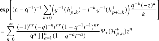 $$ \begin{align*} &\exp\left[(\mathfrak{q}-\mathfrak{q}^{-1})^{-1}\sum_{k>0}\left(\varsigma^{-1}(h_{p, k}^{\perp})-t^{-k}\varsigma^{-1}(h_{p+1, k}^{\perp})\right)\frac{q^{-k} (-z)^{ k}}{k} \right]\\ &= \sum_{n=0}^\infty\frac{(-1)^{nr}(-q)^{-n}t^{nr}(1-q^{-1}t^{-1})^{nr}}{\mathfrak{q}^n\prod_{a=1}^n(1-q^{-a}t^{-a})}\Psi_+(\mathcal{H}_{p,n}^+)z^n \end{align*} $$
and
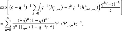 $$ \begin{align*} &\exp\left[(\mathfrak{q}-\mathfrak{q}^{-1})^{-1}\sum_{k>0}\left(\varsigma^{-1}(h_{p,- k}^{\perp})-t^{ k}\varsigma^{-1}(h_{p+1,- k}^{\perp})\right)\frac{q^{ k} (-z)^{- k}}{k} \right]\\ &= \sum_{n=0}^\infty\frac{(-q)^n(1-qt)^{nr}}{\mathfrak{q}^n\prod_{a=1}^n(1-q^{-a}t^{-a})}\Psi_-(\mathcal{H}_{p,n}^-)z^{-n}, \end{align*} $$
where
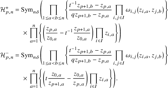 $$ \begin{align} \begin{aligned} \mathcal{H}^+_{p,n}&= \mathrm{Sym}_{n\delta}\left( \prod_{1\le a<b\le n}\left\{\frac{t^{-1}z_{p+1,b}-z_{p,a}}{qz_{p+1,b}-z_{p,a}}\prod_{i,j\in I}\omega_{i,j}\left( z_{i,a},z_{j,b} \right)\right\}\right.\\ &\ \quad\times \left.\prod_{a=1}^n\left\{\left( \frac{z_{p,a}}{z_{0,a}}-t^{-1}\frac{z_{p+1,a}}{z_{0,a}} \right)\prod_{i\in I}z_{i,a} \right\} \right)\\ \mathcal{H}^-_{p,n}&= \mathrm{Sym}_{n\delta}\left( \prod_{1\le a<b\le n}\left\{\frac{t^{-1}z_{p+1,b}-z_{p,a}}{qz_{p+1,b}-z_{p,a}}\prod_{i,j\in I}\omega_{i,j}\left( z_{i,a},z_{j,b} \right)\right\}\right.\\ &\ \quad\times \left.\prod_{a=1}^n\left\{\left( t\frac{z_{0,a}}{z_{p+1,a}}-\frac{z_{0,a}}{z_{p,a}} \right)\prod_{i\in I}z_{i,a} \right\} \right). \end{aligned} \end{align} $$
It is helpful to recall Remark 3.3 when making comparisons with [Reference Wen19]. The result follows from applying Proposition 4.3 to (4.8). We note that the mixing terms in 4.10 contribute a power of $\mathfrak {d}^{-r n(n-1)}$
before inverting
$\mathfrak {d}^{-r n(n-1)}$
before inverting $\mathfrak {d}$
.
$\mathfrak {d}$
.
4.2 Action on the vertex representation
For $F\in \mathcal {S}^+$
and
$F\in \mathcal {S}^+$
and $G\in \mathcal {S}^-$
, we will present a way to compute the actions of
$G\in \mathcal {S}^-$
, we will present a way to compute the actions of $\rho ^+_{\vec {c}}(\Psi _+(F))$
and
$\rho ^+_{\vec {c}}(\Psi _+(F))$
and $\rho _{\vec {c}}^-(\Psi _-(G))$
. Our approach was inspired by Lemma 3.2 of [Reference Feigin, Jimbo and Mukhin6] in the case
$\rho _{\vec {c}}^-(\Psi _-(G))$
. Our approach was inspired by Lemma 3.2 of [Reference Feigin, Jimbo and Mukhin6] in the case $r=1$
.
$r=1$
.
4.2.1 Matrix elements
The following is a consequence of computations similar to those done for Proposition 3.7:
Proposition 4.6. For $v_1,v_2\in W$
, we have
$v_1,v_2\in W$
, we have
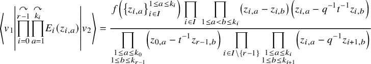 $$ \begin{align} \begin{aligned} \left\langle v_1\left| \overset{\curvearrowright}{\prod_{i=0}^{r-1}}\overset{\curvearrowright}{\prod_{a=1}^{k_i}} E_{i}(z_{i,a})\right|v_2\right\rangle &=\frac{f\left( \left\{ z_{i,a} \right\}_{i\in I}^{1\le a\le k_i} \right) \displaystyle\prod_{i\in I}\,\prod_{1\le a<b\le k_i}\left( z_{i,a}-z_{i,b} \right)\left( z_{i,a}-q^{-1}t^{-1}z_{i,b} \right)} {\displaystyle \prod_{\substack{1\le a\le k_0\\1\le b\le k_{r-1}}}\left( z_{0,a}-t^{-1}z_{r-1,b} \right) \prod_{i\in I\backslash\{r-1\}}\prod_{\substack{1\le a \le k_i\\1\le b\le k_{i+1}}}\left(z_{i,a}-q^{-1}z_{i+1,b}\right)} \end{aligned} \end{align} $$
for some Laurent polynomial f, where the rational functions are expanded into Laurent series assuming
 $$ \begin{align} |z_{i,a}|=1,\, |q|>1,\, |t|>1. \end{align} $$
However,
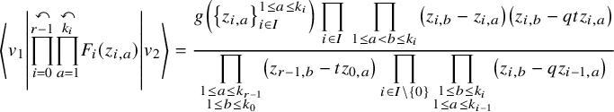 $$ \begin{align} \begin{aligned} \left\langle v_1\left| \overset{\curvearrowleft}{\prod_{i=0}^{r-1}}\overset{\curvearrowleft}{\prod_{a=1}^{k_i}} F_{i}(z_{i,a})\right|v_2\right\rangle &=\frac{g\left( \left\{ z_{i,a} \right\}_{i\in I}^{1\le a\le k_i} \right) \displaystyle\prod_{i\in I}\,\prod_{1\le a<b\le k_i}\left( z_{i,b}-z_{i,a} \right)\left( z_{i,b}-qtz_{i,a} \right)} {\displaystyle \prod_{\substack{1\le a\le k_{r-1}\\1\le b\le k_{0}}}\left( z_{r-1,b}-tz_{0,a} \right) \prod_{i\in I\backslash\{0\}}\prod_{\substack{1\le b \le k_i\\1\le a\le k_{i-1}}}\left(z_{i,b}-qz_{i-1,a}\right)} \end{aligned} \end{align} $$
for some Laurent polynomial g, where the rational functions are now expanded into Laurent series assuming
 $$ \begin{align} |z_{i,a}|=1,\, |q|<1,\, |t|<1. \end{align} $$
Notice that $\omega _{i,i+1}(z_{i,a},z_{i+1,b})^{-1}$
and
$\omega _{i,i+1}(z_{i,a},z_{i+1,b})^{-1}$
and $\omega _{i,i-1}(z_{i,a},z_{i-1,b})^{-1}$
are rational functions that we can also expand according to (4.12) and (4.14). Thus, we can make sense of matrix elements of products of currents multiplied by these inverted mixing terms. We do not claim that such products yield well-defined series of operators – just that their matrix elements make sense. The following is a consequence of the toroidal relations:
$\omega _{i,i-1}(z_{i,a},z_{i-1,b})^{-1}$
are rational functions that we can also expand according to (4.12) and (4.14). Thus, we can make sense of matrix elements of products of currents multiplied by these inverted mixing terms. We do not claim that such products yield well-defined series of operators – just that their matrix elements make sense. The following is a consequence of the toroidal relations:
Proposition 4.7. When computing matrix elements, we have the relations
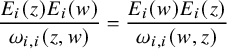 $$ \begin{align} \frac{E_{i}(z)E_i(w)}{\omega_{i,i}(z,w)}&=\frac{E_{i}(w)E_i(z)}{\omega_{i,i}(w,z)} \end{align} $$
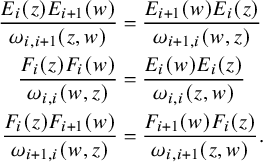 $$ \begin{align} \frac{E_{i}(z)E_{i+1}(w)}{\omega_{i,i+1}(z,w)}&= \frac{E_{i+1}(w)E_{i}(z)}{\omega_{i+1,i}(w,z)}\\ \frac{F_{i}(z)F_i(w)}{\omega_{i,i}(w,z)}&=\frac{E_{i}(w)E_i(z)}{\omega_{i,i}(z,w)}\nonumber\\ \nonumber \frac{F_{i}(z)F_{i+1}(w)}{\omega_{i+1,i}(w,z)}&= \frac{F_{i+1}(w)F_{i}(z)}{\omega_{i,i+1}(z,w)}. \end{align} $$
Proof. We will only prove the statements for $E_i(z)$
. Applying
$E_i(z)$
. Applying $\rho _{\vec {c}}^+$
to the relations from 3.1.1 yields
$\rho _{\vec {c}}^+$
to the relations from 3.1.1 yields
 $$\begin{align*}E_i(z)E_j(w)=g_{i,j}(\mathfrak{d}^{m_{i,j}}z/w)E_j(w)E_i(z). \end{align*}$$
Strictly speaking, when unpacking this relation, we should clear denominators. We then obtain
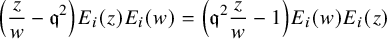 $$ \begin{align} \left(\frac{z}{w}-\mathfrak{q}^2\right)E_i(z)E_i(w)&=\left(\mathfrak{q}^2\frac{z}{w}-1\right) E_i(w)E_i(z) \end{align} $$
 $$ \begin{align} \left(\mathfrak{d}^{-1}\frac{z}{w}-\mathfrak{q}^{-1}\right)E_{i}(z)E_{i+1}(w)&=\left(\mathfrak{q}^{-1}\mathfrak{d}^{-1}\frac{z}{w}-1\right)E_{i+1}(w)E_i(z). \end{align} $$
Since $\omega _{i,i}(z,w)^{-1}=(z-\mathfrak {q}^2w)(z-w)$
, (4.17) directly yields (4.15). However, multiplying both sides of (4.18) by
$\omega _{i,i}(z,w)^{-1}=(z-\mathfrak {q}^2w)(z-w)$
, (4.17) directly yields (4.15). However, multiplying both sides of (4.18) by $-\mathfrak {q} w$
gives us
$-\mathfrak {q} w$
gives us
 $$\begin{align*}\omega_{i+1,i}(w,z)E_i(z)E_{i+1}(w)=\omega_{i,i+1}(z,w)E_{i+1}(w)E_i(z). \end{align*}$$
This implies (4.16).
4.2.2 Constant term formula
For $F\in \mathcal {S}^+_{k_{\bullet }}$
and
$F\in \mathcal {S}^+_{k_{\bullet }}$
and $G\in \mathcal {S}^-_{k_{\bullet }}$
, consider the rational functions
$G\in \mathcal {S}^-_{k_{\bullet }}$
, consider the rational functions
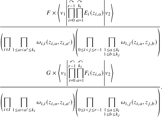 $$ \begin{align*} &\frac{\displaystyle F\times\left\langle v_1\left| \overset{\curvearrowright}{\prod_{i=0}^{r-1}}\overset{\curvearrowright}{\prod_{a=1}^{k_i}} E_{i}(z_{i,a})\right|v_2\right\rangle} {\displaystyle\left(\prod_{i\in I}\prod_{1\le a<a'\le k_i}\omega_{i,i}(z_{i,a},z_{i,a'})\right) \left(\prod_{0\le i< j\le r-1}\,\prod_{\substack{1\le a\le k_i\\1\le b\le k_j}}\omega_{i,j}(z_{i,a},z_{j,b})\right)}\\ &\frac{\displaystyle G\times\left\langle v_1\left| \overset{\curvearrowleft}{\prod_{i=0}^{r-1}}\overset{\curvearrowleft}{\prod_{a=1}^{k_i}} F_{i}(z_{i,a})\right|v_2\right\rangle} {\displaystyle\left(\prod_{i\in I}\prod_{1\le a<a'\le k_i}\omega_{i,i}(z_{i,a},z_{i,a'})\right) \left(\prod_{0\le i< j\le r-1}\,\prod_{\substack{1\le a\le k_i\\1\le b\le k_j}}\omega_{i,j}(z_{i,a},z_{j,b})\right)}. \end{align*} $$
We can expand these rational functions into Laurent series according to the assumptions (4.12) and (4.14), respectively. For any Laurent series, we denote by $\{-\}_0$
this operation of taking constant terms.
$\{-\}_0$
this operation of taking constant terms.
Lemma 4.8. For $F\in \mathcal {S}^+_{k_{\bullet }}$
and
$F\in \mathcal {S}^+_{k_{\bullet }}$
and $G\in \mathcal {S}^-_{k_{\bullet }}$
, we have
$G\in \mathcal {S}^-_{k_{\bullet }}$
, we have
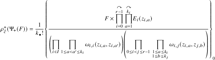 $$ \begin{align} \rho^+_{\vec{c}}(\Psi_+(F)) =\frac{1}{k_{\bullet}!}\left\{\frac{\displaystyle F\times\overset{\curvearrowright}{\prod_{i=0}^{r-1}}\,\overset{\curvearrowright}{\prod_{a=1}^{k_i}}E_i(z_{i,a})} {\displaystyle\left(\prod_{i\in I}\prod_{1\le a<a'\le k_i}\omega_{i,i}(z_{i,a},z_{i,a'})\right) \left(\prod_{0\le i< j\le r-1}\,\prod_{\substack{1\le a\le k_i\\1\le b\le k_j}}\omega_{i,j}(z_{i,a},z_{j,b})\right)}\right\}_0 \end{align} $$
where the right-hand side is expanded according to (4.12) and
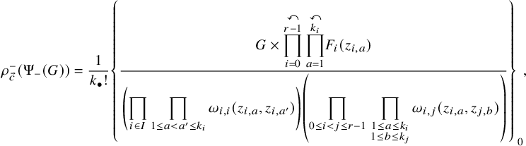 $$ \begin{align} \rho^-_{\vec{c}}(\Psi_-(G)) = \frac{1}{k_{\bullet}!}\left\{\frac{\displaystyle G\times\overset{\curvearrowleft}{\prod_{i=0}^{r-1}}\,\overset{\curvearrowleft}{\prod_{a=1}^{k_i}}F_i(z_{i,a})} {\displaystyle\left(\prod_{i\in I}\prod_{1\le a<a'\le k_i}\omega_{i,i}(z_{i,a},z_{i,a'})\right) \left(\prod_{0\le i< j\le r-1}\,\prod_{\substack{1\le a\le k_i\\1\le b\le k_j}}\omega_{i,j}(z_{i,a},z_{j,b})\right)}\right\}_0, \end{align} $$
where the right-hand side is expanded according to (4.14). In particular, the expressions on the right-hand side are well-defined operators on W.
Proof. A consequence of Theorem 4.2 and the toroidal relations is that $\mathcal {S}^{\pm }$
are both spanned by shuffle monomials
$\mathcal {S}^{\pm }$
are both spanned by shuffle monomials
 $$\begin{align*}z_{0,1}^{n(0,1)}\star z_{0,1}^{n(0,2)}\star\cdots\star z_{0,1}^{n(0,k_0)}\star z_{1,1}^{n(1,1)}\star\cdots\star z_{r-1,1}^{n(r-1,k_{r-1})} \end{align*}$$
since
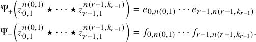 $$ \begin{align*} \Psi_+\left( z_{0,1}^{n(0,1)}\star\cdots\star z_{r-1,1}^{n(r-1,k_{r-1})} \right)&= e_{0,n(0,1)}\cdots e_{r-1,n(r-1,k_{r-1})}\\ \Psi_-\left(z_{0,1}^{n(0,1)}\star\cdots\star z_{r-1,1}^{n(r-1,k_{r-1})} \right)&= f_{0,n(0,1)}\cdots f_{r-1,n(r-1,k_{r-1})}. \end{align*} $$
We will check that the matrix elements coincide for these monomials, from which the lemma follows. For the ‘ $+$
’ case, the proposed formula gives us
$+$
’ case, the proposed formula gives us
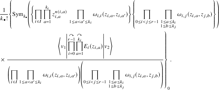 $$ \begin{align*} &\frac{1}{k_{\bullet}!}\left\{ \displaystyle\mathrm{Sym}_{k_{\bullet}}\left(\left\{\prod_{i\in I}\prod_{a=1}^{k_i}z_{i,a}^{n(i,a)} \,\prod_{1\le a<a'\le k_i}\omega_{i,i}(z_{i,a},z_{i,a'})\right\} \left\{ \prod_{0\le i<j\le r-1}\,\prod_{\substack{1\le a\le k_i\\1\le b\le k_j}}\omega_{i,j}(z_{i,a},z_{j,b}) \right\}\right)\right.\\ &\times\left.\frac{\displaystyle\left\langle v_1\left| \overset{\curvearrowright}{\prod_{i=0}^{r-1}}\overset{\curvearrowright}{\prod_{a=1}^{k_i}} E_{i}(z_{i,a})\right|v_2\right\rangle} {\displaystyle\left(\prod_{i\in I}\prod_{1\le a<a'\le k_i}\omega_{i,i}(z_{i,a},z_{i,a'})\right) \left(\prod_{0\le i< j\le r-1}\,\prod_{\substack{1\le a\le k_i\\1\le b\le k_j}}\omega_{i,j}(z_{i,a},z_{j,b})\right)}\right\}_0. \end{align*} $$
Using (4.15) to swap variables, we can move both the matrix element and the mixing terms inside the symmetrization, where the mixing terms will all cancel out. Notice that taking the constant term is insensitive to the labeling of the variables, and thus, the constant terms of all the summands of the symmetrization are equal. The end result is
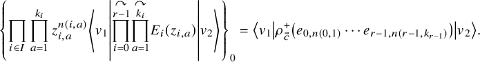 $$\begin{align*}\left\{\prod_{i\in I}\prod_{a=1}^{k_i}z_{i,a}^{n(i,a)} \left\langle v_1\left| \overset{\curvearrowright}{\prod_{i=0}^{r-1}}\overset{\curvearrowright}{\prod_{a=1}^{k_i}} E_{i}(z_{i,a})\right|v_2\right\rangle\right\}_0 =\left\langle v_1\left|\rho_{\vec{c}}^{+}\left(e_{0,n(0,1)}\cdots e_{r-1,n(r-1,k_{r-1})} \right)\right|v_2\right\rangle. \end{align*}$$
The ‘ $-$
’ case is similar.
$-$
’ case is similar.
5 Difference operators
5.1 Setup
Now, we will fix $\alpha \in Q$
, which also fixes a core. The previous two sections were concerned with symmetric functions in infinitely many variables. Here, we will shift to working with finitely many variables
$\alpha \in Q$
, which also fixes a core. The previous two sections were concerned with symmetric functions in infinitely many variables. Here, we will shift to working with finitely many variables
 $$\begin{align*}\left\{x_{l}^{(i)}\right\}_{i\in I}^{1\le l\le N_i}=X_{N_{\bullet}}. \end{align*}$$
We will impose the compatibility (2.9) between $\alpha $
and the vector
$\alpha $
and the vector $N_{\bullet }$
recording the number of variables of each color. Our approach for finding difference operators is straightforward: we use Lemma 4.8 to compute the action of
$N_{\bullet }$
recording the number of variables of each color. Our approach for finding difference operators is straightforward: we use Lemma 4.8 to compute the action of $\rho ^{\pm }_{\vec {c}}(\Psi _\pm (\mathcal {E}_{p,n}^{\pm }))$
on a function
$\rho ^{\pm }_{\vec {c}}(\Psi _\pm (\mathcal {E}_{p,n}^{\pm }))$
on a function $f\left[ X_{N_{\bullet }} \right]$
. We assume that
$f\left[ X_{N_{\bullet }} \right]$
. We assume that $n\le N_i$
for all
$n\le N_i$
for all $i\in I$
.
$i\in I$
.
5.1.1 Finitized vertex operators
Recall that $\Lambda ^I_{N_{\bullet }}$
denotes the tensor product over
$\Lambda ^I_{N_{\bullet }}$
denotes the tensor product over $i\in I$
of rings of symmetric polynomials in
$i\in I$
of rings of symmetric polynomials in $N_i$
variables and
$N_i$
variables and $\pi _{N_{\bullet }}: \Lambda ^I\to \Lambda ^I_{N_{\bullet }}$
is the natural projection. We will abuse notation and also denote the map
$\pi _{N_{\bullet }}: \Lambda ^I\to \Lambda ^I_{N_{\bullet }}$
is the natural projection. We will abuse notation and also denote the map $(\pi _{N_{\bullet }}\otimes 1):\Lambda ^I\otimes \mathbb {K}\{Q\}\rightarrow \Lambda ^I_{N_{\bullet }}\otimes \mathbb {K}\{Q\}$
by
$(\pi _{N_{\bullet }}\otimes 1):\Lambda ^I\otimes \mathbb {K}\{Q\}\rightarrow \Lambda ^I_{N_{\bullet }}\otimes \mathbb {K}\{Q\}$
by $\pi _{N_{\bullet }}$
. Recall Proposition 3.7.
$\pi _{N_{\bullet }}$
. Recall Proposition 3.7.
Remark 5.1. The action (3.7) of the operator $z^{H_i,0}$
includes a power of
$z^{H_i,0}$
includes a power of $\mathfrak {d}$
. In Proposition 3.7 and throughout this paper, we will be working with products of currents that have an equal number of
$\mathfrak {d}$
. In Proposition 3.7 and throughout this paper, we will be working with products of currents that have an equal number of $E_i(z)$
for each
$E_i(z)$
for each $i\in I$
and likewise for
$i\in I$
and likewise for $F_i(z)$
. In this setup, the powers of
$F_i(z)$
. In this setup, the powers of $\mathfrak {d}$
will cancel. Namely, because
$\mathfrak {d}$
will cancel. Namely, because $m_{i,i\pm 1}=-m_{i\pm 2,i\pm 1}$
, we have that the power of
$m_{i,i\pm 1}=-m_{i\pm 2,i\pm 1}$
, we have that the power of $\mathfrak {d}$
from the action of
$\mathfrak {d}$
from the action of $z_{i,a}^{H_{i,0}}$
will be canceled by those from the action of
$z_{i,a}^{H_{i,0}}$
will be canceled by those from the action of $z_{i\pm 2,a}^{H_{i\pm 2,0}}$
. Thus, we we will abuse notation and omit the
$z_{i\pm 2,a}^{H_{i\pm 2,0}}$
. Thus, we we will abuse notation and omit the $\mathfrak {d}$
from the action of
$\mathfrak {d}$
from the action of $z^{H_{i,0}}$
. Applying the compatibility condition (2.9), this leaves
$z^{H_{i,0}}$
. Applying the compatibility condition (2.9), this leaves
 $$\begin{align*}z^{H_{i,0}}(e^\alpha)=z^{( \alpha_i^\vee,\alpha)}=z^{N_{i}-N_{i-1}}. \end{align*}$$
Proposition 5.2. Let $f\in \Lambda ^I$
be factored according to color:
$f\in \Lambda ^I$
be factored according to color:
 $$\begin{align*}f= \prod_{i\in I} f_i[X^{(i)}], \end{align*}$$
where $f_i\in \Lambda $
for all
$f_i\in \Lambda $
for all $i\in I$
. For
$i\in I$
. For
 $$ \begin{align} |z|=1,\, |q|>1,\, |t|>1,\, |x_{l}^{(j)}|<1, \end{align} $$
the vertex operators from (3.13) act on f such that upon finitization, we have
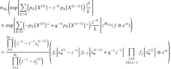 $$ \begin{align} \begin{aligned} &\pi_{N_{\bullet}} \left(\exp\left[ \sum_{k>0}\left( p_k[X^{(i)}]-t^{-k}p_k[X^{(i-1)}] \right) \frac{z^k}{k}\right]\right.\\ &\times\left.\exp\left[\sum_{k>0}\left( -p_k[X^{(i)}]^{\perp}+q^{-k}p_k[X^{(i-1)}]^{\perp} \right)\frac{z^{-k}}{k} \right]z^{H_{i,0}} (f\otimes e^\alpha)\right) \\ &= \frac{\displaystyle\prod_{l=1}^{N_{i-1}}\left(z^{-1}-t^{-1}x_{l}^{(i-1)}\right)}{\displaystyle\prod_{l=1}^{N_i} \left(z^{-1}-x_{l}^{(i)}\right)} \left( f_i\left[x_{\bullet}^{(i)}-z^{-1}\right]f_{i-1}\left[x_{\bullet}^{(i-1)}+q^{-1}z^{-1}\right] \prod_{\substack{j\in I\\j\not=i,i-1}} f_j\left[x_{\bullet}^{(j)}\right]\otimes e^\alpha\right). \end{aligned} \end{align} $$
However, for
 $$ \begin{align*} |z|=1,\, |q|<1,\, |t|<1,\, |x_{l}^{(j)}|<1, \end{align*} $$
the vertex operators from (3.15) act as
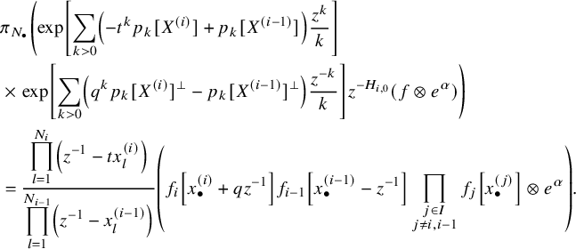 $$ \begin{align} \begin{aligned} &\pi_{N_{\bullet}} \left(\exp\left[ \sum_{k>0}\left( -t^kp_k[X^{(i)}]+p_k[X^{(i-1)}] \right) \frac{z^k}{k}\right]\right.\\ &\times \left.\exp\left[\sum_{k>0}\left( q^kp_k[X^{(i)}]^{\perp}-p_k[X^{(i-1)}]^{\perp} \right)\frac{z^{-k}}{k} \right]z^{-H_{i,0}} (f\otimes e^\alpha)\right) \\ &= \frac{\displaystyle\prod_{l=1}^{N_{i}}\left(z^{-1}-tx_{l}^{(i)}\right)} {\displaystyle\prod_{l=1}^{N_{i-1}} \left(z^{-1}-x_{l}^{(i-1)}\right)} \left( f_i\left[x_{\bullet}^{(i)}+qz^{-1}\right]f_{i-1}\left[x_{\bullet}^{(i-1)}-z^{-1}\right] \prod_{\substack{j\in I\\j\not=i,i-1}} f_j\left[x_{\bullet}^{(j)}\right]\otimes e^\alpha\right). \end{aligned} \end{align} $$
Proof. We will only consider (5.2) – the proof for (5.3) is similar. First consider the ‘left’ half of the vertex operator together with $z^{H_i,0}$
. We have
$z^{H_i,0}$
. We have
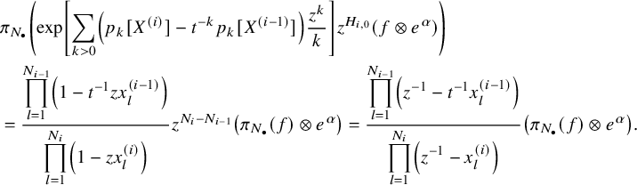 $$ \begin{align} \nonumber &\pi_{N_{\bullet}} \left(\exp\left[ \sum_{k>0}\left( p_k[X^{(i)}]-t^{-k}p_k[X^{(i-1)}] \right) \frac{z^k}{k}\right]z^{H_{i,0}} (f\otimes e^\alpha)\right) \\ &= \frac{\displaystyle\prod_{l=1}^{N_{i-1}}\left(1-t^{-1}zx_{l}^{(i-1)}\right)}{\displaystyle\prod_{l=1}^{N_i} \left(1-zx_{l}^{(i)}\right)} z^{N_i-N_{i-1}} \left( \pi_{N_{\bullet}}(f)\otimes e^\alpha\right) = \frac{\displaystyle\prod_{l=1}^{N_{i-1}}\left(z^{-1}-t^{-1}x_{l}^{(i-1)}\right)}{\displaystyle\prod_{l=1}^{N_i} \left(z^{-1}-x_{l}^{(i)}\right)} \left( \pi_{N_{\bullet}}(f)\otimes e^\alpha\right). \end{align} $$
For this to hold, we will need to impose conditions on $|x_{l}^{(i)}|$
. Recall that we have the conditions (3.14) when working with
$|x_{l}^{(i)}|$
. Recall that we have the conditions (3.14) when working with $\{E_i(z)\}$
. We extend these to (5.1) for (5.4) to hold. Let us also point out that the compatibility condition (2.9) is used to obtain the factor
$\{E_i(z)\}$
. We extend these to (5.1) for (5.4) to hold. Let us also point out that the compatibility condition (2.9) is used to obtain the factor $z^{N_i-N_{i-1}}$
after the first equality.
$z^{N_i-N_{i-1}}$
after the first equality.
Next, from the ‘right’ half, we have
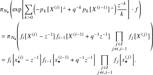 $$ \begin{align} \nonumber &\pi_{N_{\bullet}}\left( \exp\left[\sum_{k>0}\left( -p_k[X^{(i)}]^{\perp}+q^{-k}p_k[X^{(i-1)}]^{\perp} \right)\frac{z^{-k}}{k} \right]\cdot f \right)\\ &= \pi_{N_{\bullet}}\left(f_i[X^{(i)}-z^{-1}]f_{i-1}[X^{(i-1)}+q^{-1}z^{-1}]\prod_{\substack{j\in I\\j\not=i,i-1}} f_j[X^{(j)}] \right)\\ \nonumber &= f_i\left[x_{\bullet}^{(i)}-z^{-1}\right]f_{i-1}\left[x_{\bullet}^{(i-1)}+q^{-1}z^{-1}\right] \prod_{\substack{j\in I\\j\not=i,i-1}} f_j\left[x_{\bullet}^{(j)}\right].\notag \end{align} $$
Here, (5.5) follows from checking on power sums $p_k[X^{(i)}]$
and
$p_k[X^{(i)}]$
and $p_k[X^{(i-1)}]$
.
$p_k[X^{(i-1)}]$
.
Remark 5.3. As in Proposition 5.2, when writing formulas involving vertex operators, we will express them in terms of functions that are factorizable according to color:
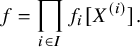 $$\begin{align*}f=\prod_{i\in I}f_i[X^{(i)}]. \end{align*}$$
Factorizable functions span $\Lambda ^I$
, so to define an operator, it suffices to consider its action on such functions. We can write our operators in terms of general f if we introduce colored plethystic notation. For instance, the terms at the bottom of (5.2) can be written as
$\Lambda ^I$
, so to define an operator, it suffices to consider its action on such functions. We can write our operators in terms of general f if we introduce colored plethystic notation. For instance, the terms at the bottom of (5.2) can be written as
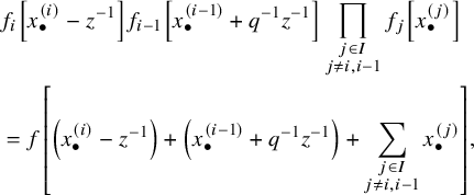 $$ \begin{align*} &f_i\left[x_{\bullet}^{(i)}-z^{-1}\right]f_{i-1}\left[x_{\bullet}^{(i-1)}+q^{-1}z^{-1}\right] \prod_{\substack{j\in I\\j\not=i,i-1}} f_j\left[x_{\bullet}^{(j)}\right]\\ &=f\left[\left(x_{\bullet}^{(i)}-z^{-1}\right)+\left(x_{\bullet}^{(i-1)}+q^{-1}z^{-1}\right)+\sum_{\substack{j\in I\\j\not=i,i-1}}x_{\bullet}^{(j)}\right], \end{align*} $$
where the bottom denotes the image of $f[X_{N_{\bullet }}]$
under the ring map generated by
$f[X_{N_{\bullet }}]$
under the ring map generated by
 $$\begin{align*}p_n[x_{\bullet}^{(j)}]\mapsto \begin{cases} p_n[x_{\bullet}^{(i)}]-z^{-n} & j=i\\ p_n[x_{\bullet}^{(i-1)}]+q^{-n}z^{-n} & j=i-1\\ p_n[x_{\bullet}^{(j)}] & \mbox{otherwise} \end{cases}. \end{align*}$$
This notation can then be carried over to general f. However, the benefits of introducing this notation in our paper seemed marginal at best, so we have elected to making statements in terms of factorizable functions.
5.1.2 Applying the constant term formula
Our next goal is to obtain constant term formulas for the action of the shuffle elements $\mathcal {E}_{p,n}^{\pm }$
from (4.9). In light of Lemma 4.4, we will also incorporate the constants
$\mathcal {E}_{p,n}^{\pm }$
from (4.9). In light of Lemma 4.4, we will also incorporate the constants
 $$ \begin{align*} c_{n}^+&:=\frac{(-1)^{n}\mathfrak{q}^{n(r-1)}t^{-n}(1-q^{-1}t^{-1})^{nr}}{v^{-n}\prod_{a=1}^n(1-q^{-a}t^{-a})},\quad c_{n}^-:=\frac{(-1)^{nr-n}\mathfrak{d}^{-n(r-1)}t^n(1-qt)^{nr}}{v^{n}q^n\prod_{a=1}^n(1-q^{-a}t^{-a})}, \end{align*} $$
where $v=(-1)^{\frac {(r-2)(r-3)}{2}}\mathfrak {q}\mathfrak {d}^{-\frac {r}{2}}(c_0\cdots c_{r-1})^{-1}$
.
$v=(-1)^{\frac {(r-2)(r-3)}{2}}\mathfrak {q}\mathfrak {d}^{-\frac {r}{2}}(c_0\cdots c_{r-1})^{-1}$
.
Lemma 5.4. For any factorizable $f=\prod _{i\in I}f_i[X^{(i)}]\in \Lambda ^I$
, we have
$f=\prod _{i\in I}f_i[X^{(i)}]\in \Lambda ^I$
, we have
 $$ \begin{align} \begin{aligned} &c_n^+ \pi_{N_{\bullet}}\bigg( (\rho_{\vec{c}}^+\circ\Psi_+)(\mathcal{E}_{p,n}^+)(f\otimes e^\alpha)\bigg)\\ &=\frac{(1-q^{-1}t^{-1})^{nr}}{t^{n}\prod_{a=1}^n(1-q^{-a}t^{-a})} \left\{\prod_{i\in I}\prod_{a=1}^n\prod_{l=1}^{N_i}\left(\frac{ z_{i+1,a}^{-1}-t^{-1}x_{l}^{(i)} }{ z_{i,a}^{-1}-x_{l}^{(i)} }\right)\right.\\ &\times\prod_{1\le a<b\le n} \left[ \frac{\left(1-z_{p+1,b}/z_{p+1,a}\right)\left(1-q^{-1}t^{-1}z_{p+1,b}/z_{p+1,a}\right)}{\left(1-tz_{p,b}/z_{p+1,a}\right)\left(1-t^{-1}z_{p+2,b}/z_{p+1,a}\right)}\right.\\ &\times\left.\prod_{i\in I\backslash\{p+1\}} \frac{\left(1-z_{i,b}/z_{i,a}\right)\left(1-q^{-1}t^{-1}z_{i,b}/z_{i,a}\right)}{\left(1-q^{-1}z_{i-1,b}/z_{i,a}\right)\left(1-t^{-1}z_{i+1,b}/z_{i,a}\right)}\right]\\ &\times\prod_{a=1}^n \left[ \left(\frac{z_{0,a}}{z_{p,a}}\right)\left(\frac{1}{1-t^{-1}z_{p+1,a}/z_{p,a}}\right)\right.\\ &\times\left. \prod_{i\in I\setminus\{p+1\}} \left(\frac{1}{1-t^{-1}z_{i,a}/z_{i-1,a}}\right) \left( \frac{1}{1-q^{-1}z_{i-1,a}/z_{i,a}} \right)\right]\\ &\left.\times \prod_{i\in I} f_i\left[ \sum_{l=1}^{N_i} x_{l}^{(i)}-\sum_{a=1}^nz_{i,a}^{-1}+q^{-1}\sum_{a=1}^n z_{i+1,a}^{-1} \right] \right\}_0\otimes e^\alpha \end{aligned} \end{align} $$
and
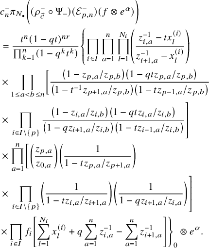 $$ \begin{align} \begin{aligned} &c_n^-\pi_{N_{\bullet}}\bigg((\rho_{\vec{c}}^-\circ\Psi_-)(\mathcal{E}_{p,n}^-)(f\otimes e^\alpha)\bigg)\\ &=\frac{t^n(1-qt)^{nr}}{\prod_{k=1}^n(1-q^kt^k)} \left\{\prod_{i\in I}\prod_{a=1}^n\prod_{l=1}^{N_i}\left(\frac{ z_{i,a}^{-1}-tx_{l}^{(i)} }{ z_{i+1,a}^{-1}-x_{l}^{(i)} }\right)\right.\\ &\times\prod_{1\le a<b\le n}\left[ \frac{\left(1-z_{p,a}/z_{p,b}\right)\left(1-qtz_{p,a}/z_{p,b}\right)}{\left(1-t^{-1}z_{p+1,a}/z_{p,b}\right)\left(1-tz_{p-1,a}/z_{p,b}\right)}\right.\\ &\times\left. \prod_{i\in I\backslash\{p\}} \frac{\left(1-z_{i,a}/z_{i,b}\right)\left(1-qtz_{i,a}/z_{i,b}\right)}{\left(1-qz_{i+1,a}/z_{i,b}\right)\left(1-tz_{i-1,a}/z_{i,b}\right)}\right]\\ &\times \prod_{a=1}^n\left[ \left(\frac{z_{p,a}}{z_{0,a}}\right)\left(\frac{1}{1-tz_{p,a}/z_{p+1,a}}\right)\right.\\ &\times\left. \prod_{i\in I\setminus\{p\}} \left(\frac{1}{1-tz_{i,a}/z_{i+1,a}}\right) \left( \frac{1}{1-qz_{i+1,a}/z_{i,a}} \right) \right]\\ &\left.\times \prod_{i\in I} f_i\left[ \sum_{l=1}^{N_i} x_{l}^{(i)}+q\sum_{a=1}^n z_{i,a}^{-1}-\sum_{a=1}^n z_{i+1,a}^{-1} \right]\right\}_0\otimes e^\alpha. \end{aligned} \end{align} $$
Proof. Plugging in $\mathcal {E}_{p,n}^{\pm }$
into the formula from Lemma 4.8, we can use the toroidal relations and Proposition 4.7 to reorder the currents in alignment with Proposition 3.7. As in the proof of Lemma 4.8, we can use the toroidal relations to remove the symmetrizations in
$\mathcal {E}_{p,n}^{\pm }$
into the formula from Lemma 4.8, we can use the toroidal relations and Proposition 4.7 to reorder the currents in alignment with Proposition 3.7. As in the proof of Lemma 4.8, we can use the toroidal relations to remove the symmetrizations in $\mathcal {E}_{p,n}^{\pm }$
. Taking the result for
$\mathcal {E}_{p,n}^{\pm }$
. Taking the result for $\mathcal {E}_{p,n}^+$
, acting on
$\mathcal {E}_{p,n}^+$
, acting on $f\otimes e^\alpha $
and then applying
$f\otimes e^\alpha $
and then applying $\pi _{N_{\bullet }}$
gives us
$\pi _{N_{\bullet }}$
gives us
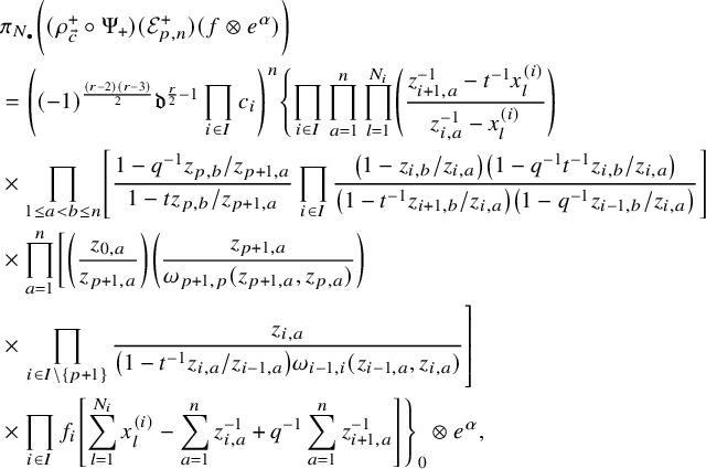 $$ \begin{align*} \begin{aligned} &\pi_{N_{\bullet}}\bigg( (\rho_{\vec{c}}^+\circ\Psi_+)(\mathcal{E}_{p,n}^+)(f\otimes e^\alpha)\bigg)\\ &=\left( (-1)^{\frac{(r-2)(r-3)}{2}}\mathfrak{d}^{\frac{r}{2}-1}\prod_{i\in I} c_i\right)^n \left\{\prod_{i\in I}\prod_{a=1}^n\prod_{l=1}^{N_i}\left(\frac{ z_{i+1,a}^{-1}-t^{-1}x_{l}^{(i)} }{ z_{i,a}^{-1}-x_{l}^{(i)} }\right)\right.\\ &\times\prod_{1\le a<b\le n} \left[ \frac{1-q^{-1}z_{p,b}/z_{p+1,a}}{1-tz_{p,b}/z_{p+1,a}} \prod_{i\in I} \frac{\left(1-z_{i,b}/z_{i,a}\right)\left(1-q^{-1}t^{-1}z_{i,b}/z_{i,a}\right)}{\left(1-t^{-1}z_{i+1,b}/z_{i,a}\right)\left(1-q^{-1}z_{i-1,b}/z_{i,a}\right)} \right]\\ &\times\prod_{a=1}^n \left[\left(\frac{z_{0,a}}{z_{p+1,a}}\right)\left(\frac{z_{p+1,a}}{\omega_{p+1,p}(z_{p+1,a},z_{p,a})}\right)\right.\\ &\times\left.\prod_{i\in I\setminus\{p+1\}} \frac{z_{i,a}}{\left(1-t^{-1}z_{i,a}/z_{i-1,a}\right)\omega_{i-1,i}(z_{i-1,a},z_{i,a})}\right]\\ &\times \prod_{i\in I}f_i\left[ \sum_{l=1}^{N_i}x_{l}^{(i)}-\sum_{a=1}^nz_{i,a}^{-1}+q^{-1}\sum_{a=1}^n z_{i+1,a}^{-1} \right]\Bigg\}_0\otimes e^\alpha, \end{aligned} \end{align*} $$
where all rational functions are expanded as Laurent series assuming
 $$ \begin{align} |z_{i,a}|=1,\, |x_{l}^{(j)}|<1,\, |t|>1,\, |q|>1. \end{align} $$
For $\mathcal {E}_{p,n}^-$
, we instead have
$\mathcal {E}_{p,n}^-$
, we instead have
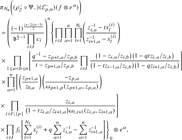 $$ \begin{align*} \begin{aligned} &\pi_{N_{\bullet}}\bigg((\rho_{\vec{c}}^-\circ\Psi_-)(\mathcal{E}_{p,n}^-) (f\otimes e^\alpha)\bigg)\\ &= \left( \frac{(-1)^{\frac{(r-2)(r-3)}{2}}}{\displaystyle\mathfrak{d}^{\frac{r}{2}-1} \prod_{i\in I} c_i}\right)^n \left\{\prod_{i\in I}\prod_{a=1}^n\prod_{l=1}^{N_i}\left(\frac{ z_{i,a}^{-1}-tx_{l}^{(i)} }{ z_{i+1,a}^{-1}-x_{l}^{(i)} }\right)\right.\\ &\times\prod_{1\le a<b\le n} \left[ \frac{q^{-1}-z_{p+1,a}/z_{p,b}}{t-z_{p+1,a}/z_{p,b}} \prod_{i\in I} \frac{\left(1-z_{i,a}/z_{i,b}\right)\left(1-qtz_{i,a}/z_{i,b}\right)}{\left(1-tz_{i-1,a}/z_{i,b}\right)\left(1-qz_{i+1,a}/z_{i,b}\right)} \right]\\ &\times \prod_{a=1}^n \left[ \left(\frac{z_{p+1,a}}{z_{0,a}}\right) \left(\frac{-z_{p,a}} {\omega_{p+1,p}(z_{p+1,a},z_{p,a})}\right)\right.\\ &\left.\times\prod_{i\in I\setminus\{p\}} \frac{z_{i,a}}{\left(1-tz_{i,a}/z_{i+1,a}\right)\omega_{i,i+1}(z_{i,a},z_{i+1,a})} \right]\\ &\left.\times \prod_{i\in I}f_i\left[ \sum_{l=1}^{N_i} x_{l}^{(i)}+q\sum_{a=1}^n z_{i,a}^{-1}-\sum_{a=1}^n z_{i+1,a}^{-1} \right]\right\}_0\otimes e^\alpha, \end{aligned} \end{align*} $$
where all rational functions are expanded into Laurent series assuming.
 $$ \begin{align} |z_{i,a}|=1,\, |x_{l}^{(j)}|<1,\, |q|<1,\, |t|<1. \end{align} $$
In both formulas, we are taking constant terms in the z-variables.
Finally, to obtain (5.6) and (5.7) from these formulas, we multiply through by $c_n^{\pm }$
and use
$c_n^{\pm }$
and use $q=\mathfrak {q}\mathfrak {d}, t=\mathfrak {q}\mathfrak {d}^{-1}$
to write
$q=\mathfrak {q}\mathfrak {d}, t=\mathfrak {q}\mathfrak {d}^{-1}$
to write
 $$ \begin{align*} \omega_{i,i+1}(z,w)&= \mathfrak{q} w-\mathfrak{d}^{-1}z=\mathfrak{d}^{-1}(qw-z)=\mathfrak{q}\left(w-q^{-1}z\right)\\ \omega_{i,i-1}(z,w)&= z-\mathfrak{q}\mathfrak{d}^{-1}w=z-tw.\\[-38pt] \end{align*} $$
Remark 5.5. Observe that the formulas in Lemma 5.4 are for symmetric functions in finitely many variables. To obtain constant term formulas for operators in infinitely many variables, we can apply Proposition 5.2. For example, starting from (5.6), we use (5.2) and replace
 $$\begin{align*}\prod_{i\in I}\prod_{a=1}^n\prod_{l=1}^{N_i}\left(\frac{ z_{i+1,a}^{-1}-t^{-1}x_{l}^{(i)} }{ z_{i,a}^{-1}-x_{l}^{(i)} }\right) f_i\left[ \sum_{l=1}^{N_i} x_{l}^{(i)}-\sum_{a=1}^nz_{i,a}^{-1}+q^{-1}\sum_{a=1}^n z_{i+1,a}^{-1} \right] \otimes e^\alpha \end{align*}$$
with
 $$ \begin{align*} &\exp\left[ \sum_{i\in I}\sum_{a=1}^n\left(\sum_{k>0}\left( p_k[X^{(i)}]-t^{-k}p_k[X^{(i-1)}] \right) \frac{z_{i,a}^k}{k}\right)\right]\\ &\times\exp\left[\sum_{i\in I}\sum_{a=1}^n\sum_{k>0}\left( -p_k[X^{(i)}]^{\perp}+q^{-k}p_k[X^{(i-1)}]^{\perp} \right)\frac{z_{i,a}^{-k}}{k} \right]z^{H_{i,0}} (f\otimes e^\alpha). \end{align*} $$
5.1.3 Integral formula
Regardless of f, the formulas obtained in 5.1.2 are constant terms of Laurent series expansions of some rational function. Note that all poles are simple except for the poles at zero possibly coming from the plethystic modifications done to f. Thus, it will be advantageous to invert all the z-variables: let
 $$\begin{align*}w_{i,a}:=z_{i,a}^{-1} \end{align*}$$
and define the functions
 $$ \begin{align} g_{p,n}^+(w_{\bullet,\bullet},X_{N_{\bullet}}) &:=\frac{(-1)^{\frac{n(n-1)}{2}}(1-q^{-1}t^{-1})^{nr}}{t^{\frac{n(n+1)}{2}}\prod_{a=1}^n(1-q^{-a}t^{-a})} \prod_{i\in I}\prod_{a=1}^n\prod_{l=1}^{N_i}\left(\frac{ w_{i+1,a}-t^{-1}x_{l}^{(i)} }{ w_{i,a}-x_{l}^{(i)} }\right) \end{align} $$
 $$ \begin{align} &\times\prod_{1\le a<b\le n} \left[ \frac{\left(w_{p+1,b}-w_{p+1,a}\right)\left(w_{p+1,b}-q^{-1}t^{-1}w_{p+1,a}\right)} {\left(w_{p+1,a}-t^{-1}w_{p,b}\right)\left(w_{p+2,b}-t^{-1}w_{p+1,a}\right)}\right. \end{align} $$
 $$ \begin{align} &\times\left. \prod_{i\in I\backslash\{p+1\}} \frac{\left(w_{i,b}-w_{i,a}\right)\left(w_{i,b}-q^{-1}t^{-1}w_{i,a}\right)}{\left(w_{i-1,b}-q^{-1}w_{i,a}\right)\left(w_{i+1,b}-t^{-1}w_{i,a}\right)}\right] \end{align} $$
 $$ \begin{align} &\times\prod_{a=1}^n \left[ \left(\frac{w_{p,a}}{w_{0,a}}\right)\left(\frac{w_{p+1,a}}{w_{p+1,a}-t^{-1}w_{p,a}}\right)\right. \end{align} $$
 $$ \begin{align} &\times\left. \prod_{i\in I\setminus\{p+1\}} \left(\frac{w_{i,a}}{w_{i,a}-t^{-1}w_{i-1,a}}\right) \left( \frac{w_{i-1,a}}{w_{i-1,a}-q^{-1}w_{i,a}} \right)\right] \end{align} $$
and
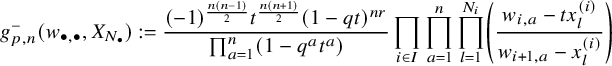 $$ \begin{align} g_{p,n}^-(w_{\bullet,\bullet},X_{N_{\bullet}}) &:= \frac{(-1)^{\frac{n(n-1)}{2}}t^{\frac{n(n+1)}{2}}(1-qt)^{nr}}{\prod_{a=1}^n(1-q^at^a)} \prod_{i\in I}\prod_{a=1}^n\prod_{l=1}^{N_i}\left(\frac{ w_{i,a}-tx_{l}^{(i)} }{ w_{i+1,a}-x_{l}^{(i)} }\right) \end{align} $$
 $$ \begin{align} &\times\prod_{1\le a<b\le n}\left[ \frac{\left(w_{p,a}-w_{p,b}\right)\left(w_{p,a}-qtw_{p,b}\right)}{\left(w_{p,b}-tw_{p+1,a}\right)\left(w_{p-1,a}-tw_{p,b}\right)}\right. \end{align} $$
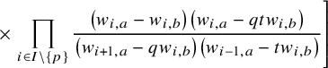 $$ \begin{align} &\times\left. \prod_{i\in I\backslash\{p\}} \frac{\left(w_{i,a}-w_{i,b}\right)\left(w_{i,a}-qtw_{i,b}\right)}{\left(w_{i+1,a}-qw_{i,b}\right)\left(w_{i-1,a}-tw_{i,b}\right)}\right] \end{align} $$
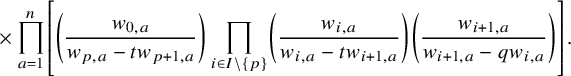 $$ \begin{align} &\times \prod_{a=1}^n\left[ \left(\frac{w_{0,a}}{w_{p,a}-tw_{p+1,a}}\right) \prod_{i\in I\setminus\{p\}} \left(\frac{w_{i,a}}{w_{i,a}-tw_{i+1,a}}\right) \left( \frac{w_{i+1,a}}{w_{i+1,a}-qw_{i,a}} \right) \right]. \end{align} $$
Lemma 5.6. Let $f=\prod _{i\in I} f_i[X^{(i)}]\in \Lambda ^I$
be factorizable according to color. For the ‘+’ case, assume
$f=\prod _{i\in I} f_i[X^{(i)}]\in \Lambda ^I$
be factorizable according to color. For the ‘+’ case, assume
 $$\begin{align*}|x_{l}^{(i)}|<1,\, |q|>1,\, |t|>1. \end{align*}$$
We have
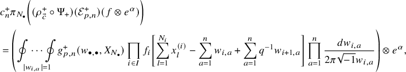 $$ \begin{align} \nonumber &c_n^+ \pi_{N_{\bullet}}\bigg( (\rho_{\vec{c}}^+\circ\Psi_+)(\mathcal{E}_{p,n}^+)(f\otimes e^\alpha)\bigg)\\ &=\left(\underset{|w_{i,a}|=1}{\oint\cdots\oint}g_{p,n}^+(w_{\bullet,\bullet},X_{N_{\bullet}}) \prod_{i\in I} f_i\left[ \sum_{l=1}^{N_i} x_{l}^{(i)}-\sum_{a=1}^nw_{i,a}+\sum_{a=1}^{n}q^{-1}w_{i+1,a} \right] \prod_{a=1}^n \frac{dw_{i,a}}{2\pi\sqrt{-1}w_{i,a}} \right)\otimes e^\alpha, \end{align} $$
where we orient the unit circle $|w_{i,a}|=1$
counter-clockwise. In the ‘
$|w_{i,a}|=1$
counter-clockwise. In the ‘ $-$
’ case, we now assume
$-$
’ case, we now assume
 $$\begin{align*}|x_{l}^{(i)}|<1,\, |q|<1,\, |t|<1. \end{align*}$$
We then have
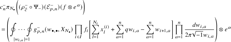 $$ \begin{align} \nonumber &c_n^- \pi_{N_{\bullet}}\bigg( (\rho_{\vec{c}}^-\circ\Psi_-)(\mathcal{E}_{p,n}^-)(f\otimes e^\alpha)\bigg)\\ &=\left(\underset{|w_{i,a}|=1}{\oint\cdots\oint}g_{p,n}^-(w_{\bullet,\bullet},X_{N_{\bullet}}) \prod_{i\in I} f_i\left[ \sum_{l=1}^{N_i} x_{l}^{(i)}+\sum_{a=1}^nqw_{i,a}-\sum_{a=1}^nw_{i+1,a} \right] \prod_{a=1}^n \frac{dw_{i,a}}{2\pi\sqrt{-1}w_{i,a}} \right)\otimes e^\alpha \end{align} $$
and also orient the unit circle counter-clockwise.
Proof. Upon making the substitution $w_{i,a}:=z_{i,a}^{-1}$
, the right-hand side of (5.6) is equal to
$w_{i,a}:=z_{i,a}^{-1}$
, the right-hand side of (5.6) is equal to
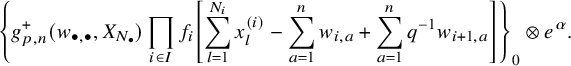 $$ \begin{align} \left\{g_{p,n}^+(w_{\bullet,\bullet},X_{N_{\bullet}})\prod_{i\in I}f_i\left[\sum_{l=1}^{N_i} x_{l}^{(i)}-\sum_{a=1}^nw_{i,a}+\sum_{a=1}^nq^{-1}w_{i+1,a} \right]\right\}_0\otimes e^\alpha. \end{align} $$
Now, all the poles appearing in (5.21) are simple. Similarly, the right-hand side of (5.7) becomes
 $$ \begin{align} \left\{g_{p,n}^-(w_{\bullet,\bullet},X_{N_{\bullet}})\prod_{i\in I}f_i\left[ \sum_{l=1}^{N_i}x_{l}^{(i)}+\sum_{a=1}^nqw_{i,a}- \sum_{a=1}^nw_{i+1,a} \right]\right\}_0\otimes e^\alpha. \end{align} $$
In case ‘ $\pm $
’, the integrands are given by series in the
$\pm $
’, the integrands are given by series in the $x^{(i)}_l$
and
$x^{(i)}_l$
and $q^{\mp 1}$
,
$q^{\mp 1}$
, $t^{\mp 1}$
, with coefficients which are Laurent polynomials in the
$t^{\mp 1}$
, with coefficients which are Laurent polynomials in the $w_{i,a}$
. Under the given assumptions, these series converge uniformly absolutely on the integration cycle, and thus, we can exchange the order of summation and integration. This turns the integrals (5.19) and (5.20) into the constant term formulas (5.21) and (5.22), respectively.
$w_{i,a}$
. Under the given assumptions, these series converge uniformly absolutely on the integration cycle, and thus, we can exchange the order of summation and integration. This turns the integrals (5.19) and (5.20) into the constant term formulas (5.21) and (5.22), respectively.
Remark 5.7. Recall that the compatibility condition (2.9) between $N_{\bullet }$
and
$N_{\bullet }$
and $\alpha $
was used to obtain the formulas in Proposition 5.2. At this stage, we note that without the compatibility, we would have to contend with an additional Laurent monomial factor in the variables
$\alpha $
was used to obtain the formulas in Proposition 5.2. At this stage, we note that without the compatibility, we would have to contend with an additional Laurent monomial factor in the variables $w_{i,a}$
in (5.21) and (5.22). This would prevent us from obtaining a manageable formula due to the presence of non-simple poles at zero.
$w_{i,a}$
in (5.21) and (5.22). This would prevent us from obtaining a manageable formula due to the presence of non-simple poles at zero.
5.1.4 Cyclic-shift operators
To describe the results of our computation, we need to introduce some difference operators that also permute variables. As before, let $X_{N_{\bullet }}=\{x_{l}^{(i)}\}_{i\in I}^{1\le l\le N_i}$
denote our set of variables compatible with our r-core via (2.9). Define a shift pattern of
$X_{N_{\bullet }}=\{x_{l}^{(i)}\}_{i\in I}^{1\le l\le N_i}$
denote our set of variables compatible with our r-core via (2.9). Define a shift pattern of $X_{N_{\bullet }}$
to be a subset of
$X_{N_{\bullet }}$
to be a subset of $X_{N_{\bullet }}$
that contains no more than one variable of each color. A shift pattern contains color
$X_{N_{\bullet }}$
that contains no more than one variable of each color. A shift pattern contains color $p\in I$
if it contains a variable of color p. Let
$p\in I$
if it contains a variable of color p. Let $Sh_p(X_{N_{\bullet }})$
denote the set of all shift patterns containing color p.
$Sh_p(X_{N_{\bullet }})$
denote the set of all shift patterns containing color p.
For a shift pattern ${\underline {J}}$
, let
${\underline {J}}$
, let $J\subset I$
denote the colors of the variables in
$J\subset I$
denote the colors of the variables in ${\underline {J}}$
. We denote the variables in
${\underline {J}}$
. We denote the variables in ${\underline {J}}$
by
${\underline {J}}$
by $x_{{\underline {J}}}^{(i)}$
, so
$x_{{\underline {J}}}^{(i)}$
, so ${\underline {J}}=\{ x_{{\underline {J}}}^{(i)} \}_{i\in J}$
. To
${\underline {J}}=\{ x_{{\underline {J}}}^{(i)} \}_{i\in J}$
. To $\underline {J}$
we associate the following:
$\underline {J}$
we associate the following:
-
1. Gap labels: For
$i\in I$
, let
$i^{\vartriangle }\in J$
be first element greater than or equal to i in the cyclic order. Similarly, let
$i^{\triangledown }\in J$
be the first element less than or equal to i in the cyclic order. We stipulate that
$0\le i^{\vartriangle }-i, i-i^{\triangledown }\le r-1$
. With this set, we define
$$ \begin{align*} x_{{\underline{J}}^\vartriangle}^{(i)}&=q^{(i-i^{\vartriangle})}x_{{\underline{J}}}^{(i^\vartriangle)}\\ x_{{\underline{J}}^\triangledown}^{(i)}&=q^{(i-i^{\triangledown})}x_{{\underline{J}}}^{(i^\triangledown)}. \end{align*} $$
To clarify,
$x_{{\underline {J}}^\vartriangle }^{(i)}=x_{{\underline {J}}^\triangledown }^{(i)}=x_{{\underline {J}}}^{(i)}$
if
$i\in J$
. Thus, while
${\underline {J}}$
gives a list of variables colored by
$J\subset I$
, we ‘fill in the gaps’ for values
$i\in I\backslash J$
with certain q-shifts of the elements of
${\underline {J}}$
. Note that the q-shifts are negative for
$x_{{\underline {J}}^\vartriangle }^{(i)}$
and positive for
$x_{{\underline {J}}^\triangledown }^{(i)}$
. -
2. A cyclic-shift operator: For
$i\in J$
, let
$i^{\blacktriangledown }\in J$
be the first element strictly less than i in the cyclic order. We set
$1\le i-i^\blacktriangledown \le r$
, where r occurs if and only if
$|J|=\{i\}$
. We then define the operator
$T_{{\underline {J}}}$
on
$\mathbb {K}[X_{N_{\bullet }}]$
as the algebra map induced by
$$ \begin{align*} T_{{\underline{J}}}(x_{l}^{(i)})&= \left\{ \begin{array}{ll} q^{(i-i^\blacktriangledown)}x_{{\underline{J}}}^{(i^\blacktriangledown)} & \text{if } i\in J \text{ and } x_{l}=x_{{\underline{J}}}^{(i)} \\ x_{l}^{(i)}&\mbox{otherwise.} \end{array} \right. \end{align*} $$
Note that this q-shift is positive. If we let
$i^{\blacktriangle }\in J$
be the first element strictly greater than i in the cyclic order, then observe that
$$ \begin{align*} T^{-1}_{{\underline{J}}}(x_{l}^{(i)})&= \left\{ \begin{array}{ll} q^{(i-i^\blacktriangle)}x_{{\underline{J}}}^{(i^\blacktriangle)} & \text{if } i\in J \text{ and } x_{l}^{(i)}=x_{{\underline{J}}}^{(i)} \\ x_{l}^{(i)}&\mbox{otherwise}, \end{array} \right. \end{align*} $$
where as before, we view
$1\le i^{\blacktriangle }-i\le r$
. Finally, we note the following: for
$i\in J$
, (5.23)
$$ \begin{align} \begin{aligned} T_{\underline{J}}(x_{{\underline{J}}}^{(i)})&= qx_{{\underline{J}}^\triangledown}^{(i-1)}\\ T_{\underline{J}}^{-1}(x_{{\underline{J}}}^{(i)})&= q^{-1}x_{{\underline{J}}^\vartriangle}^{(i+1)}. \end{aligned} \end{align} $$


The cyclic-shift operators $T_{{\underline {J}}}^{\pm 1}$
will arise when evaluating the integrals of Lemma 5.6 by iterated residues. For later use, and to clarify this relationship, we record the following:
$T_{{\underline {J}}}^{\pm 1}$
will arise when evaluating the integrals of Lemma 5.6 by iterated residues. For later use, and to clarify this relationship, we record the following:
Lemma 5.8. For any $f=\prod _i f_i[X^{(i)}]\in \Lambda ^I$
,
$f=\prod _i f_i[X^{(i)}]\in \Lambda ^I$
, ${\underline {J}}\in Sh_p(X_{N_{\bullet }})$
, define the following evaluations on a set of auxilliary variables
${\underline {J}}\in Sh_p(X_{N_{\bullet }})$
, define the following evaluations on a set of auxilliary variables $\{w_i\}_{i\in I}$
:
$\{w_i\}_{i\in I}$
:
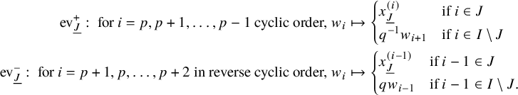 $$ \begin{align*} \mathrm{ev}_{{\underline{J}}}^+ : \ \text{for } i=p,p+1,\dotsc,p-1 \text{ cyclic order,} \ w_i &\mapsto \begin{cases} x^{(i)}_{{\underline{J}}} & \text{if } i\in J\\ q^{-1}w_{i+1} & \text{if } i\in I\setminus J \end{cases}\\ \mathrm{ev}_{{\underline{J}}}^- : \ \text{for } i=p+1,p,\dotsc,p+2 \text{ in reverse cyclic order,} \ w_i &\mapsto \begin{cases} x^{(i-1)}_{{\underline{J}}} & \text{if } i-1\in J\\ qw_{i-1} & \text{if } i-1\in I\setminus J. \end{cases} \end{align*} $$
We then have
 $$ \begin{align} \begin{aligned} \mathrm{ev}_{{\underline{J}}}^+(w_i)&= x_{{\underline{J}}^\vartriangle}^{(i)},& \mathrm{ev}_{{\underline{J}}}^-(w_i)&= x_{{\underline{J}}^\triangledown}^{(i)} \end{aligned} \end{align} $$
and
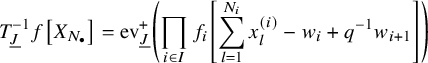 $$ \begin{align} T_{{\underline{J}}}^{-1}f\left[X_{N_{\bullet}}\right] &= \mathrm{ev}_{{\underline{J}}}^+\left( \prod_{i\in I} f_i\left[ \sum_{l=1}^{N_i} x_{l}^{(i)}-w_{i}+q^{-1}w_{i+1} \right] \right) \end{align} $$
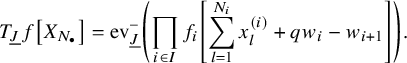 $$ \begin{align} T_{{\underline{J}}}f\left[X_{N_{\bullet}}\right] &= \mathrm{ev}_{{\underline{J}}}^-\left( \prod_{i\in I} f_i\left[ \sum_{l=1}^{N_i} x_{l}^{(i)}+qw_{i}-w_{i+1} \right] \right). \end{align} $$
Proof. The equations (5.24) follow from the definitions. Equipped with that, the right-hand side of (5.25) becomes
 $$\begin{align*}\prod_{i\in I}f_i\left[\sum_{l=1}^{N_i} x_i^{(i)}-x_{{\underline{J}}^\vartriangle}^{(i)}+q^{-1}x_{{\underline{J}}^\vartriangle}^{(i+1)}\right] \end{align*}$$
If $i\in I\backslash J$
, then
$i\in I\backslash J$
, then $x_{{\underline {J}}^\vartriangle }^{(i)}=q^{-1}x_{{\underline {J}}^\vartriangle }^{(i+1)}$
and so
$x_{{\underline {J}}^\vartriangle }^{(i)}=q^{-1}x_{{\underline {J}}^\vartriangle }^{(i+1)}$
and so $f_i$
is unchanged. However, if
$f_i$
is unchanged. However, if $i\in J$
, then
$i\in J$
, then $x_{{\underline {J}}^\vartriangle }^{(i)}=x_{{\underline {J}}}^{(i)}$
and we obtain
$x_{{\underline {J}}^\vartriangle }^{(i)}=x_{{\underline {J}}}^{(i)}$
and we obtain $T_{{\underline {J}}}^{-1}f_i$
by (5.23). The case of (5.26) is similar.
$T_{{\underline {J}}}^{-1}f_i$
by (5.23). The case of (5.26) is similar.
Example 5.9. For instance, suppose $r=3$
,
$r=3$
, $p=0$
, and
$p=0$
, and ${\underline {J}}=\{x^{(0)}_1,x^{(2)}_1\}$
. Then the right-hand side of (5.25) is
${\underline {J}}=\{x^{(0)}_1,x^{(2)}_1\}$
. Then the right-hand side of (5.25) is
 $$ \begin{align*}\mathrm{ev}_{{\underline{J}}}^+\left(f_{0}\left[ \sum_{l=1}^{N_{0}} x_{l}^{(0)}-w_0+q^{-1}w_{1} \right] f_1\left[ \sum_{l=1}^{N_1} x_{l}^{(1)}-w_{1}+q^{-1}w_{2} \right] f_{2}\left[ \sum_{l=1}^{N_{2}} x_{l}^{(2)}-w_{2}+q^{-1}w_0 \right]\right) \end{align*} $$
with $\mathrm {ev}_{{\underline {J}}}^+$
given by evaluating
$\mathrm {ev}_{{\underline {J}}}^+$
given by evaluating $w_0\mapsto x^{(0)}_1,w_1\mapsto q^{-1}w_2,w_2\mapsto x^{(2)}_1$
in this order. The result is
$w_0\mapsto x^{(0)}_1,w_1\mapsto q^{-1}w_2,w_2\mapsto x^{(2)}_1$
in this order. The result is
 $$ \begin{align*}f_{0}\left[ \sum_{l=1}^{N_{0}} x_{l}^{(0)}-x^{(0)}_1+q^{-2}x^{(2)}_1 \right] f_1\left[ \sum_{l=1}^{N_1} x_{l}^{(1)}+0\right] f_{2}\left[ \sum_{l=1}^{N_{2}} x_{l}^{(2)}-x^{(2)}_1+q^{-1}x^{(0)}_1\right] = T_{{\underline{J}}}^{-1}f\left[X_{N_{\bullet}}\right]. \end{align*} $$
We will also make use of n-tuples of shift patterns. For such an n-tuple $\mathbf {\underline {J}}=(\underline {J}_1,\ldots , \underline {J}_n)$
and
$\mathbf {\underline {J}}=(\underline {J}_1,\ldots , \underline {J}_n)$
and $0\le k\le n$
, we denote
$0\le k\le n$
, we denote
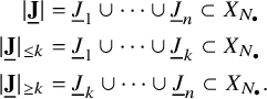 $$ \begin{align*} |\mathbf{\underline{J}}|&=\underline{J}_1\cup\cdots\cup\underline{J}_n\subset X_{N_{\bullet}}\\ |\mathbf{\underline{J}}|_{\le k}&=\underline{J}_1\cup\cdots\cup\underline{J}_{k}\subset X_{N_{\bullet}}\\ |\mathbf{\underline{J}}|_{\ge k}&=\underline{J}_k\cup\cdots\cup\underline{J}_{n}\subset X_{N_{\bullet}}. \end{align*} $$
If $\mathbf {\underline {J}}$
is an n-tuple of shift patterns all containing color p, we say
$\mathbf {\underline {J}}$
is an n-tuple of shift patterns all containing color p, we say $\mathbf {\underline {J}}$
is p-distinct if the p-colored variables
$\mathbf {\underline {J}}$
is p-distinct if the p-colored variables $x_{\underline {J}_k}^{(p)}$
are all distinct. Let
$x_{\underline {J}_k}^{(p)}$
are all distinct. Let $Sh_p^{[n]}(X_{N_{\bullet }})$
denote the set of all p-distinct n-tuples of shift patterns containing color p.
$Sh_p^{[n]}(X_{N_{\bullet }})$
denote the set of all p-distinct n-tuples of shift patterns containing color p.
5.2 Degree one case
We will first compute the integrals from Lemma 5.6 for the case $n=1$
. The first order wreath Macdonald operators are defined as follows:
$n=1$
. The first order wreath Macdonald operators are defined as follows:
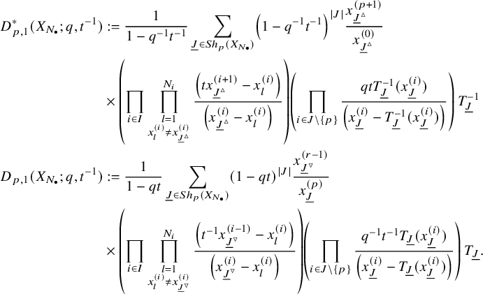 $$ \begin{align*} D_{p,1}^*(X_{N_{\bullet}};q,t^{-1}) &:= \frac{1}{1-q^{-1}t^{-1}} \sum_{{\underline{J}}\in Sh_p(X_{N_{\bullet}})} \left( 1-q^{-1}t^{-1} \right)^{|J|} \frac{x^{(p+1)}_{{\underline{J}}^\vartriangle}}{x_{{\underline{J}}^\vartriangle}^{(0)}}\\ &\times \left(\prod_{i\in I} \prod_{\substack{l=1\\x_{l}^{(i)}\not= x^{(i)}_{{\underline{J}}^\vartriangle}}}^{N_i} \frac{\left(t x^{(i+1)}_{{\underline{J}}^\vartriangle}-x^{(i)}_{l} \right)} {\left( x^{(i)}_{{\underline{J}}^\vartriangle}-x^{(i)}_{l} \right)}\right) \left(\prod_{i\in J\backslash\left\{ p \right\}} \frac{qtT_{\underline{J}}^{-1}(x^{(i)}_{{\underline{J}}})}{\left( x^{(i)}_{{\underline{J}}}-T_{\underline{J}}^{-1}(x^{(i)}_{{\underline{J}}}) \right)}\right)\ T_{\underline{J}}^{-1}\\D_{p,1}(X_{N_{\bullet}}; q, t^{-1}) &:= \frac{1}{1-qt} \sum_{{\underline{J}}\in Sh_{p}(X_{N_{\bullet}})}\left( 1-qt \right)^{|J|} \frac{x^{(r-1)}_{{\underline{J}}^\triangledown}}{x^{(p)}_{{\underline{J}}}}\\ &\times \left(\prod_{i\in I} \prod_{\substack{l=1\\x^{(i)}_{l}\not= x^{(i)}_{{\underline{J}}^\triangledown}}}^{N_i} \frac{\left( t^{-1}x^{(i-1)}_{{\underline{J}}^\triangledown}-x^{(i)}_{l} \right)} {\left( x^{(i)}_{{\underline{J}}^\triangledown}-x^{(i)}_{l} \right)}\right) \left(\prod_{i\in J\backslash\left\{ p \right\}} \frac{q^{-1}t^{-1}T_{\underline{J}}(x^{(i)}_{{\underline{J}}})}{\left( x^{(i)}_{{\underline{J}}}-T_{\underline{J}} (x^{(i)}_{{\underline{J}}}) \right)}\right)\ T_{\underline{J}}. \end{align*} $$
Observe that when $r=1$
,
$r=1$
, $D_{0,1}(x_{0,\bullet };q,t)$
and
$D_{0,1}(x_{0,\bullet };q,t)$
and $D_{0,1}^*(x_{0,\bullet };q,t)$
are the first Macdonald and dual Macdonald operators, respectively.
$D_{0,1}^*(x_{0,\bullet };q,t)$
are the first Macdonald and dual Macdonald operators, respectively.
Proposition 5.10. The integrals from Lemma 5.6 for $n=1$
yield the following:
$n=1$
yield the following:
-
$(+)$
For we have
$$\begin{align*}|x_{l}^{(i)}|<1,\, |q|\gg1,\, |t|\gg1, \end{align*}$$
$$ \begin{align*} c_1^+ \pi_{N_{\bullet}}\bigg( (\rho_{\vec{c}}^+\circ\Psi_+)(\mathcal{E}_{p,1}^+)(f\otimes e^\alpha)\bigg) = \left(t^{-|N_{\bullet}|}D_{p,1}^*(X_{N_{\bullet}};q,t^{-1})+\frac{t^{-p-1-|N_{\bullet}|}}{1-t^{-r}}\right)f\left[ X_{N_{\bullet}} \right]. \end{align*} $$
-
$(-)$
For we have
$$\begin{align*}|x_{l}^{(i)}|<1,\, |q|\ll 1,\, |t|\ll 1, \end{align*}$$
$$ \begin{align*} c_1^- \pi_{N_{\bullet}}\bigg( (\rho_{\vec{c}}^-\circ\Psi_-)(\mathcal{E}_{p,1}^-)(f\otimes e^\alpha)\bigg) = \left(t^{|N_{\bullet}|}D_{p,1}(X_{N_{\bullet}};q,t^{-1})+\frac{t^{p+1+|N_{\bullet}|}}{1-t^{r}}\right)f\left[ X_{N_{\bullet}} \right]. \end{align*} $$


Proof. In the ‘ $+$
’ case, the integral from Lemma 5.6 is
$+$
’ case, the integral from Lemma 5.6 is
 $$ \begin{align} &t^{-1}(1-q^{-1}t^{-1})^{r-1} \underset{|w_{i,1}|=1}{\oint\cdots\oint} \prod_{i\in I}\prod_{l=1}^{N_i} \frac{\left( w_{i+1,1}-t^{-1}x_{l}^{(i)} \right)} {\left( w_{i,1}-x_{l}^{(i)} \right)} \end{align} $$
 $$ \begin{align} &\times \left( \frac{w_{p,1}}{w_{0,1}} \right) \left( \frac{w_{p+1,1}}{w_{p+1,1}-t^{-1}w_{p,1}} \right) \prod_{i\in I\backslash \{p+1\}} \left( \frac{w_{i,1}}{w_{i,1}-t^{-1}w_{i-1,1}} \right) \left( \frac{w_{i-1,1}}{w_{i-1,1}-q^{-1}w_{i,1}} \right) \end{align} $$
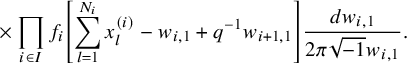 $$ \begin{align} &\times \prod_{i\in I} f_i\left[ \sum_{l=1}^{N_i}x_{l}^{(i)}-w_{i,1}+q^{-1}w_{i+1,1} \right] \frac{dw_{i,1}}{2\pi \sqrt{-1}w_{i,1}}. \end{align} $$
We will first integrate $w_{p,1}$
. Based on (5.8), the residues within the unit circle
$w_{p,1}$
. Based on (5.8), the residues within the unit circle $|w_{p,1}|=1$
come from the factors
$|w_{p,1}|=1$
come from the factors
 $$\begin{align*}\frac{1}{\underbrace{\left( w_{p,1}-t^{-1}w_{p-1,1} \right)}_{(5.28)} \underbrace{\prod_{l=1}^{N_p}\left( w_{p,1}-x_{l}^{(p)} \right)}_{(5.27)}}. \end{align*}$$
We will call the first type of pole a t-pole and the second type an x-pole.
The ‘ $-$
’ case is
$-$
’ case is
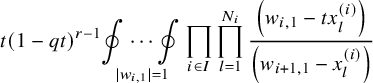 $$ \begin{align} &t(1-qt)^{r-1} \underset{|w_{i,1}|=1}{\oint\cdots\oint} \prod_{i\in I}\prod_{l=1}^{N_i} \frac{\left( w_{i,1}-tx_{l}^{(i)} \right)} {\left( w_{i+1,1}-x_{l}^{(i)} \right)} \end{align} $$
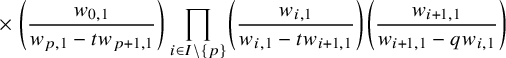 $$ \begin{align} &\times \left(\frac{w_{0,1}} {w_{p,1}-tw_{p+1,1}} \right) \prod_{i\in I\backslash\left\{ p \right\}} \left( \frac{w_{i,1}}{w_{i,1}-tw_{i+1,1}} \right) \left( \frac{w_{i+1,1}}{w_{i+1,1}-qw_{i,1}} \right) \end{align} $$
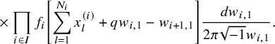 $$ \begin{align} &\times \prod_{i\in I} f_i\left[ \sum_{l=1}^{N_i}x_{l}^{(i)}+qw_{i,1}-w_{i+1,1} \right] \frac{dw_{i,1}}{2\pi \sqrt{-1}w_{i,1}}. \end{align} $$
Here, we will instead start by integrating $w_{p+1,1}$
. As before, there are x-poles and a t-pole coming from
$w_{p+1,1}$
. As before, there are x-poles and a t-pole coming from
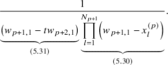 $$\begin{align*}\frac{1}{ \underbrace{\left( w_{p+1,1}-tw_{p+2,1} \right)}_{(5.31)} \underbrace{\prod_{l=1}^{N_{p+1}}\left( w_{p+1,1}-x_{l}^{(p)} \right)}_{(5.30)}}. \end{align*}$$
Our analysis of the integrals at these two kinds of poles is addressed in 5.2.1 and 5.2.2 below.
5.2.1 The t-poles
First consider the ‘ $+$
’ case. Here, we begin with the residue
$+$
’ case. Here, we begin with the residue $w_{p,1}=t^{-1}w_{p-1,1}$
. Let us group together the factors
$w_{p,1}=t^{-1}w_{p-1,1}$
. Let us group together the factors
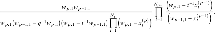 $$\begin{align*}\frac{w_{p,1}w_{p-1,1}}{w_{p,1}\left( w_{p-1,1}-q^{-1}w_{p,1} \right)\left( w_{p,1}-t^{-1}w_{p-1,1} \right) \displaystyle \prod_{l=1}^{N_p}\left( w_{p,1}-x_{l}^{(p)} \right)} \prod_{l=1}^{N_{p-1}}\frac{\left( w_{p,1}-t^{-1}x_{l}^{(p-1)} \right)} {\left( w_{p-1,1}-x_{l}^{(p-1)} \right)}. \end{align*}$$
Upon taking taking the residue, this becomes
 $$\begin{align*}\frac{t^{-N_{p-1}}}{\left(1-q^{-1}t^{-1}\right) \displaystyle \prod_{l=1}^{N_p}\left( t^{-1}w_{p-1,1}-x_{l}^{(p)} \right)}. \end{align*}$$
Because of the additional restriction $|t|\gg 1$
, the poles above will be outside the unit circle
$|t|\gg 1$
, the poles above will be outside the unit circle $|w_{p-1,1}|=1$
.
$|w_{p-1,1}|=1$
.
This pattern persists as we continue downwards in cyclic order until we reach $w_{p+1,1}$
. Here, we have
$w_{p+1,1}$
. Here, we have
 $$ \begin{align*} &\left. \frac{w_{p+1,1}w_{p,1}}{w_{p+1,1}w_{0,1} \left( w_{p+1,1}-t^{-1}w_{p,1} \right)} \right|_{\substack{w_{0,1}\mapsto t^{p+1-r}w_{p+1,1}\\ w_{p,1}\mapsto t^{-(r-1)}w_{p+1,1}}} \prod_{l=1}^{N_{p}} \frac{\left( w_{p+1,1}-t^{-1}x_{l}^{(p)} \right)} {\left( t^{-r+1}w_{p+1,1}-x_{l}^{(p)} \right)}\\ &= \frac{t^{-p}}{1-t^{-r}} \cdot\frac{1}{w_{p+1,1}}\prod_{l=1}^{N_{p}} \frac{\left( w_{p+1,1}-t^{-1}x_{l}^{(p)} \right)} {\left( t^{-r+1}w_{p+1,1}-x_{l}^{(p)} \right)}. \end{align*} $$
The only pole here is the simple pole at $w_{p+1,1}=0$
. After taking this residue, (5.29) becomes just
$w_{p+1,1}=0$
. After taking this residue, (5.29) becomes just $f\left[ X_{N_{\bullet }} \right]$
. Bringing in the front matter in (5.27), we are left with
$f\left[ X_{N_{\bullet }} \right]$
. Bringing in the front matter in (5.27), we are left with
 $$ \begin{align*} \frac{t^{-p-1-|N_{\bullet}|}} {1- t^{-r } } f\left[ X_{N_{\bullet}} \right]. \end{align*} $$
Here, we recall that $N_{\bullet }=(N_0,\ldots , N_{r-1})$
records the number of x-variables and
$N_{\bullet }=(N_0,\ldots , N_{r-1})$
records the number of x-variables and $|N_{\bullet }|=\sum _{i\in I}N_i$
.
$|N_{\bullet }|=\sum _{i\in I}N_i$
.
For the ‘ $-$
’ case, recall that we begin at
$-$
’ case, recall that we begin at $w_{p+1,1}$
and take the residue
$w_{p+1,1}$
and take the residue $w_{p+1,1}=tw_{p+2}$
. We group together the factors
$w_{p+1,1}=tw_{p+2}$
. We group together the factors
 $$\begin{align*}\frac{w_{p+1,1}w_{p+2,1}}{w_{p+1,1}\left( w_{p+2,1}-qw_{p+1,1} \right)\left( w_{p+1,1}-tw_{p+2,1} \right) \displaystyle \prod_{l=1}^{N_p}\left( w_{p+1,1}-x_{l}^{(p)} \right)} \prod_{l=1}^{N_{p+1}} \frac{\left( w_{p+1,1}-tx_{l}^{(p+1)} \right)} {\left( w_{p+1,2}-x_{l}^{(p+1)} \right)}, \end{align*}$$
which upon taking the residue becomes
 $$\begin{align*}\frac{t^{N_{p+1}}}{\left( 1-qt \right) \displaystyle \prod_{l=1}^{N_p}\left( tw_{p+2,1}-x_{l}^{(p)} \right)}. \end{align*}$$
The remaining poles above lie outside the unit circle $|w_{p+2,1}|=1$
because we have assumed
$|w_{p+2,1}|=1$
because we have assumed $|t|\ll 1$
. We continue upwards in cyclic order, yielding similar calculations until we arrive at
$|t|\ll 1$
. We continue upwards in cyclic order, yielding similar calculations until we arrive at $w_{p,1}$
. Here, we have the factors
$w_{p,1}$
. Here, we have the factors
 $$ \begin{align*} &\left.\frac{w_{0,1}} {w_{p,1}\left( w_{p,1}-tw_{p+1,1} \right)}\right|_{\substack{w_{0,1}\mapsto t^p w_{p,1}\\w_{p+1,1}\mapsto t^{r-1}w_{p,1}}} \prod_{l=1}^{N_p} \frac{\left( w_{p,1}-tx_{l}^{(p)} \right)} {\left( t^{r-1}w_{p,1}-x_{l}^{(p)} \right)}\\ &= \frac{t^p}{1-t^r} \cdot \frac{1}{w_{p,1}} \prod_{l=1}^{N_p} \frac{\left( w_{p,1}-tx_{l}^{(p)} \right)} {\left( t^{r-1}w_{p,1}-x_{l}^{(p)} \right)}. \end{align*} $$
The only pole within the unit circle $|w_{p,1}|=1$
is
$|w_{p,1}|=1$
is $w_{p,1}=0$
. After taking this residue, the final result (after including the front matter) is
$w_{p,1}=0$
. After taking this residue, the final result (after including the front matter) is
 $$ \begin{align*} \frac{t^{p+1+|N_{\bullet}|}}{1-t^r}f\left[ X_{N_{\bullet}} \right]. \end{align*} $$
5.2.2 The x-poles
We will first work out the ‘ $+$
’ case. Thus, we have taken the residue of
$+$
’ case. Thus, we have taken the residue of $w_{p,1}$
at the pole
$w_{p,1}$
at the pole $w_{p,1}=x_{l}^{(p)}$
for some
$w_{p,1}=x_{l}^{(p)}$
for some $1\le l \le N_p$
. This variable
$1\le l \le N_p$
. This variable $x_{l}^{(p)}$
will be an element of a shift pattern
$x_{l}^{(p)}$
will be an element of a shift pattern ${\underline {J}}$
. Therefore, we call it
${\underline {J}}$
. Therefore, we call it $x_{{\underline {J}}}^{(p)}$
. It will be advantageous to now group together the factors
$x_{{\underline {J}}}^{(p)}$
. It will be advantageous to now group together the factors
 $$\begin{align*}\frac{\displaystyle w_{p,1}w_{p+1,1}} {w_{0,1}w_{p,1}\left( w_{p+1,1}-t^{-1}w_{p,1} \right)} \prod_{l=1}^{N_{p}} \frac{\left( w_{p+1,1}-t^{-1}x_{l}^{(p)} \right)} {\left( w_{p,1}-x_{l}^{(p)} \right)}. \end{align*}$$
After taking the residue, we leave behind
 $$\begin{align*}\frac{w_{p+1,1}}{w_{0,1}} \prod_{\substack{l=1\\x_{l}^{(p)}\not=x_{{\underline{J}}}^{(p)}}}^{N_{p}} \frac{\left( w_{p+1,1}-t^{-1}x_{1}^{(p)} \right)} {\left( x_{{\underline{J}}}^{(p)}-x_{l}^{(p)} \right)}. \end{align*}$$
Next, we consider $w_{p+1,1}$
. We group together the factors
$w_{p+1,1}$
. We group together the factors
 $$\begin{align*}\frac{ w_{p+1,1}w_{p+2,1}} {w_{p+1,1} \left( w_{p+2,1}-t^{-1}w_{p+1,1} \right) \underbrace{\left( w_{p+1,1}-q^{-1}w_{p+2,1} \right)}_{(1)} } \prod_{l=1}^{N_{p+1}} \frac{\left( w_{p+2,1}-t^{-1}x_{l}^{(p+1)} \right)} {\underbrace{\left( w_{p+1,1}-x_{l}^{(p+1)} \right)}_{(2)}}. \end{align*}$$
The only (nonremovable) poles within the unit circle $|w_{p+1,1}|=1$
are marked (1) and (2). We thus have two cases:
$|w_{p+1,1}|=1$
are marked (1) and (2). We thus have two cases:
-
1. Residue at
$w_{p+1,1}=q^{-1}w_{p+2,1}$
: In this case,
$\left( w_{p+2,1}-t^{-1}w_{p+1,1} \right)$
cancels with a
$w_{p+2,1}$
in the numerator, leaving behind
$$\begin{align*}\frac{1} {\left(1 -q^{-1}t^{-1} \right)} \left. \prod_{l=1}^{N_{p+1}} \frac{ \left( w_{p+2,1}-t^{-1}x_{l}^{(p+1)} \right)} {\left( w_{p+1,1}-x_{l}^{(p+1)} \right)}\right|_{w_{p+1,1}\mapsto q^{-1}w_{p+2,1}}. \end{align*}$$
Because
$|q|\gg 1$
, the poles above lie outside the unit circle
$|w_{p+2,1}|=1$
. -
2. Residue at
$w_{p+1,1}=x_{l}^{(p+1)}=:x_{{\underline {J}}}^{(p+1)}$
: Here,
$\left( w_{p+2,1}-t^{-1}w_{p+1,1} \right)$
cancels with a factor in the numerator, leaving behind (5.33)
$$ \begin{align} \frac{w_{p+2,1}}{\left(x_{{\underline{J}}}^{(p+1)}-q^{-1}w_{p+2,1}\right)} \prod_{\substack{l=1\\x_{l}^{(p+1)}\not=x_{{\underline{J}}}^{(p+1)}}}^{N_{p+1}} \frac{\left( w_{p+2,1}-t^{-1}x_{1}^{(p+1)} \right)} {\left( x_{{\underline{J}}}^{(p+1)}-x_{l}^{(p+1)} \right)}. \end{align} $$
Again, because
$|q|\gg 1$
, the first pole above lies outside the unit circle
$|w_{p+2,1}|=1$
.


This pattern and dichotomy for residues continues upwards in cyclic order. The x-variables in the type (2) residues constitute a shift pattern ${\underline {J}}$
, and our gap labels
${\underline {J}}$
, and our gap labels $x_{{\underline {J}}^\vartriangle }^{(i)}$
incorporate the q-shifts from the type (1) residues. Therefore,
$x_{{\underline {J}}^\vartriangle }^{(i)}$
incorporate the q-shifts from the type (1) residues. Therefore, $w_{i,1}$
is always evaluated at
$w_{i,1}$
is always evaluated at $x_{{\underline {J}}^\vartriangle }^{(i)}$
. Finally, observe that by Lemma 5.8, (5.29) becomes
$x_{{\underline {J}}^\vartriangle }^{(i)}$
. Finally, observe that by Lemma 5.8, (5.29) becomes $T_{{\underline {J}}}^{-1}f\left[ X_{N_{\bullet }} \right]$
. The end result is
$T_{{\underline {J}}}^{-1}f\left[ X_{N_{\bullet }} \right]$
. The end result is $t^{-|N_{\bullet }|}D_{p,1}^*(q,t^{-1})f\left[ X_{N_{\bullet }} \right]$
.
$t^{-|N_{\bullet }|}D_{p,1}^*(q,t^{-1})f\left[ X_{N_{\bullet }} \right]$
.
The ‘ $-$
’ case is similar. Our first variable is
$-$
’ case is similar. Our first variable is $w_{p+1,1}$
, for which we take the residue at
$w_{p+1,1}$
, for which we take the residue at $w_{p+1,1}=x_{l}^{(p)}=:x_{{\underline {J}}}^{(p)}$
. We consider the factors
$w_{p+1,1}=x_{l}^{(p)}=:x_{{\underline {J}}}^{(p)}$
. We consider the factors
 $$\begin{align*}\left(\frac{w_{0,1}}{w_{p+1,1}} \right) \frac{1}{\left(w_{p,1}-tw_{p+1,1}\right)} \prod_{l=1}^{N_p} \frac{\left(w_{p,1}-tx_{l}^{(p)} \right)} {\left( w_{p+1,1}-x_{l}^{(p)} \right)}. \end{align*}$$
After taking the residue, the pole from $(w_{p,1}-tw_{p+1,1})$
cancels with a factor in the numerator, leaving behind
$(w_{p,1}-tw_{p+1,1})$
cancels with a factor in the numerator, leaving behind
 $$\begin{align*}\frac{w_{0,1}}{x_{{\underline{J}}}^{(p)}} \prod_{\substack{l=1\\x_{l}^{(p)}\not=x_{{\underline{J}}}^{(p)}}}^{N_p} \frac{\left(w_{p,1}-tx_{l}^{(p)} \right)} {\left( x_{{\underline{J}}}^{(p)}-x_{l}^{(p)} \right)}. \end{align*}$$
We now proceed downward in cyclic order. For each $w_{i,1}$
, we consider the factors
$w_{i,1}$
, we consider the factors
 $$\begin{align*}\frac{w_{i,1}w_{i-1,1}} {w_{i,1}\left( w_{i-1,1}-tw_{i,1} \right)\underbrace{\left( w_{i,1}-qw_{i-1,1} \right)}_{(1)}} \prod_{l=1}^{N_{i-1}} \frac{\left( w_{i-1,1}-tx_{l}^{(i-1)} \right)} {\underbrace{\left( w_{i,1}-x_{l}^{(i-1)} \right)}_{(2)}}. \end{align*}$$
Because $\left( w_{i,1}-tw_{i+1,1} \right)$
has been canceled at this point, the only poles within the unit circle
$\left( w_{i,1}-tw_{i+1,1} \right)$
has been canceled at this point, the only poles within the unit circle $|w_{i,1}|=1$
are those marked (1) and (2). The analysis is as before:
$|w_{i,1}|=1$
are those marked (1) and (2). The analysis is as before:
-
1. Residue at
$w_{i,1}=qw_{i-1,1}$
: This leaves behind
$$\begin{align*}\frac{1}{(1-qt)} \prod_{l=1}^{N_{i-1}} \left. \frac{\left( w_{i-1,1}-tx_{l}^{(i-1)} \right)} {\left( w_{i,1}-x_{l}^{(i-1)} \right)}\right|_{w_{i,1}\mapsto qw_{i-1,1}}. \end{align*}$$
-
2. Residue at
$w_{i,1}=x_{l}^{(i-1)}=:x_{{\underline {J}}}^{(i-1)}$
: The leftovers are now (5.34)
$$ \begin{align} \frac{w_{i-1,1}}{\left( x_{i-1,{\underline{J}}}-qw_{i-1,1} \right)} \prod_{\substack{l=1\\x_{l}^{(i-1)}\not=x_{{\underline{J}}}^{(i-1)}}}^{N_{i-1}} \frac{\left( w_{i-1,1}-tx_{l}^{(i-1)} \right)} {\left( x_{{\underline{J}}}^{(i-1)}-x_{l}^{(i-1)} \right)}. \end{align} $$


The x-variables where we have taken residues constitute a shift pattern ${\underline {J}}$
, and
${\underline {J}}$
, and $w_{i,1}$
is always evaluated at
$w_{i,1}$
is always evaluated at $x_{{\underline {J}}^\triangledown }^{(i-1)}$
. Again, by Lemma 5.8, (5.32) becomes
$x_{{\underline {J}}^\triangledown }^{(i-1)}$
. Again, by Lemma 5.8, (5.32) becomes $T_{{\underline {J}}}f\left[ X_{N_{\bullet }} \right]$
. Here, we obtain
$T_{{\underline {J}}}f\left[ X_{N_{\bullet }} \right]$
. Here, we obtain $t^{|N_{\bullet }|}D_{p,1}(q,t^{-1})f\left[ X_{N_{\bullet }} \right]$
.
$t^{|N_{\bullet }|}D_{p,1}(q,t^{-1})f\left[ X_{N_{\bullet }} \right]$
.
5.2.3 Degree one eigenfunction equation
Finally, we enhance Proposition 5.10 by obtaining eigenfunction equations for $D_{p,1}^*(q,t)$
and
$D_{p,1}^*(q,t)$
and $D_{p,1}(q,t)$
for generic values of the parameters.
$D_{p,1}(q,t)$
for generic values of the parameters.
Theorem 5.11. For generic values of q, t,
 $$ \begin{align} D_{p,1}^*\left( X_{N_{\bullet}};q,t \right)P_{\lambda}[X_{N_{\bullet}};q,t] &=\left(\sum_{\substack{b=1\\ b-\lambda_b\equiv p+1}}^{|N_{\bullet}|} q^{-\lambda_b}t^{-|N_{\bullet}|+b}\right) P_{\lambda}[X_{N_{\bullet}};q,t] \end{align} $$
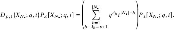 $$ \begin{align} D_{p,1}\left( X_{N_{\bullet}};q,t \right)P_{\lambda}[X_{N_{\bullet}};q,t] &=\left(\sum_{\substack{b=1\\ b-\lambda_b\equiv p+1}}^{|N_{\bullet}|} q^{\lambda_b}t^{|N_{\bullet}|-b}\right) P_{\lambda}[X_{N_{\bullet}};q,t]. \end{align} $$
Proof. We will only consider the ‘ $+$
’ case – the ‘
$+$
’ case – the ‘ $-$
’ case is similar. Combining Lemma 3.11 and Proposition 5.10, we have for
$-$
’ case is similar. Combining Lemma 3.11 and Proposition 5.10, we have for $\lambda \in \mathbb {Y}$
with
$\lambda \in \mathbb {Y}$
with $\kappa (\lambda )=\alpha $
and
$\kappa (\lambda )=\alpha $
and $|\mathrm {quot}(\lambda )|\le |N_{\bullet }|$
,
$|\mathrm {quot}(\lambda )|\le |N_{\bullet }|$
,
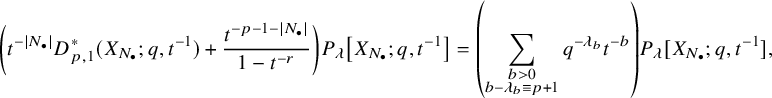 $$ \begin{align*} \left(t^{-|N_{\bullet}|}D_{p,1}^*(X_{N_{\bullet}};q,t^{-1})+\frac{t^{-p-1-|N_{\bullet}|}}{1-t^{-r}}\right)P_{\lambda}\left[ X_{N_{\bullet}}; q,t^{-1} \right] &= \left(\sum_{\substack{b>0\\ b-\lambda_b\equiv p+1}} q^{-\lambda_b}t^{-b}\right) P_{\lambda}[X_{N_{\bullet}}; q,t^{-1}], \end{align*} $$
where we assume $|q|\gg 1$
,
$|q|\gg 1$
, $|t|\gg 1$
and
$|t|\gg 1$
and $|x_{i,l}|<1$
. Even here, it is essential that
$|x_{i,l}|<1$
. Even here, it is essential that $|t|\gg 1$
as we are working with series in
$|t|\gg 1$
as we are working with series in $t^{-1}$
. We can do away with this once we notice that since
$t^{-1}$
. We can do away with this once we notice that since $|N_{\bullet }|$
is divisible by r (Proposition 2.7) and
$|N_{\bullet }|$
is divisible by r (Proposition 2.7) and $\ell (\lambda )\le |N_{\bullet }|$
,
$\ell (\lambda )\le |N_{\bullet }|$
,
 $$ \begin{align} \begin{aligned} \sum_{\substack{b>0\\ b-\lambda_b\equiv p+1}} q^{-\lambda_b}t^{-b} &= \left(\sum_{k=0}^\infty t^{-p-1-|N_{\bullet}|-rk}\right)+ \left(\sum_{\substack{b=1\\ b-\lambda_b\equiv p+1}}^{|N_{\bullet}|} q^{-\lambda_b}t^{-b}\right)\\[8pt] &=\frac{t^{-p-1-|N_{\bullet}|}}{1-t^{-r}}+\left(\sum_{\substack{b=1\\ b-\lambda_b\equiv p+1}}^{|N_{\bullet}|} q^{-\lambda_b}t^{-b}\right). \end{aligned} \end{align} $$
Here, we have split off the terms corresponding to rows above height $|N_{\bullet }|$
. Thus, (5.36) holds under our conditions on
$|N_{\bullet }|$
. Thus, (5.36) holds under our conditions on $|q|$
,
$|q|$
, $|t|$
and
$|t|$
and $|x_{l}^{(i)}|$
.
$|x_{l}^{(i)}|$
.
Finally, we address the genericity of parameters. The equations (5.35) and (5.36) are equalities of rational functions in the space $(X_{N_{\bullet }}, q,t)$
. We have established them over an analytic open subset of
$(X_{N_{\bullet }}, q,t)$
. We have established them over an analytic open subset of $(X_{N_{\bullet }}, q,t)$
. After subtracting one side to the other, this is equivalent saying a rational function is zero on a codimension zero subspace, and thus, it must be zero.
$(X_{N_{\bullet }}, q,t)$
. After subtracting one side to the other, this is equivalent saying a rational function is zero on a codimension zero subspace, and thus, it must be zero.
The eigenvalues of $\left\{ D_{p,1}(X_{N_{\bullet }};q,t) \right\}_{p\in I}$
on
$\left\{ D_{p,1}(X_{N_{\bullet }};q,t) \right\}_{p\in I}$
on $\left\{ P_{\lambda }[X_{N_{\bullet }};q,t] \right\}$
are nondegenerate. Therefore, we have the following:
$\left\{ P_{\lambda }[X_{N_{\bullet }};q,t] \right\}$
are nondegenerate. Therefore, we have the following:
Corollary 5.12. For $\lambda $
with core
$\lambda $
with core $\kappa (\lambda )$
compatible with
$\kappa (\lambda )$
compatible with $N_{\bullet }$
(cf. 2.9), the line spanned by
$N_{\bullet }$
(cf. 2.9), the line spanned by $P_{\lambda }[X_{N_{\bullet }};q,t]$
is characterized by the eigenfunction equations (5.35) ranging over all
$P_{\lambda }[X_{N_{\bullet }};q,t]$
is characterized by the eigenfunction equations (5.35) ranging over all $p\in I$
.
$p\in I$
.
Example 5.13. Let $r=3$
,
$r=3$
, $p=1$
,
$p=1$
, $N_{\bullet }=(2,1,0)$
and
$N_{\bullet }=(2,1,0)$
and $\lambda =(3,1,1)$
. In this case,
$\lambda =(3,1,1)$
. In this case, $\lambda $
is a
$\lambda $
is a $3$
-core and so
$3$
-core and so
 $$\begin{align*}P_{\lambda}[X_{N_{\bullet}};q,t]=1.\end{align*}$$
There are three shift patterns containing $p=1$
:
$p=1$
:
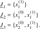 $$ \begin{align*} {\underline{J}}_1&=\{x_1^{(1)}\}\\ {\underline{J}}_2&=\{x_1^{(0)},x_1^{(1)}\}\\ {\underline{J}}_3&=\{x_2^{(0)},x_1^{(1)}\}. \end{align*} $$
The operator $D_{1,1}(X_{N_{\bullet }};q,t)$
is then
$D_{1,1}(X_{N_{\bullet }};q,t)$
is then
 $$ \begin{align} D_{1,1}(X_{N_{\bullet}};q,t)&=q\left(\frac{qtx_1^{(1)}-x_1^{(0)}}{q^2x_1^{(1)}-x_1^{(0)}}\right)\left(\frac{qtx_1^{(1)}-x_2^{(0)}}{q^2x_1^{(1)}-x_2^{(0)}}\right)T_{{\underline{J}}_1} \end{align} $$
 $$ \begin{align} &+(1-qt^{-1})q\left(\frac{qtx_1^{(1)}-x_2^{(0)}}{x_1^{(0)}-x_2^{(0)}}\right)\left(\frac{qtx_1^{(1)}}{x_1^{(0)}-q^2x_1^{(1)}}\right)T_{{\underline{J}}_2} \end{align} $$
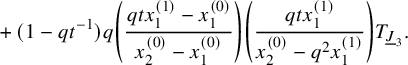 $$ \begin{align} &+(1-qt^{-1})q\left(\frac{qtx_1^{(1)}-x_1^{(0)}}{x_2^{(0)}-x_1^{(0)}}\right)\left(\frac{qtx_1^{(1)}}{x_2^{(0)}-q^2x_1^{(1)}}\right)T_{{\underline{J}}_3}. \end{align} $$
The cyclic-shift operators act trivially on $P_{\lambda }(X_{N_{\bullet }};q,t)$
. Consolidating (5.39) and (5.40) gets us
$P_{\lambda }(X_{N_{\bullet }};q,t)$
. Consolidating (5.39) and (5.40) gets us
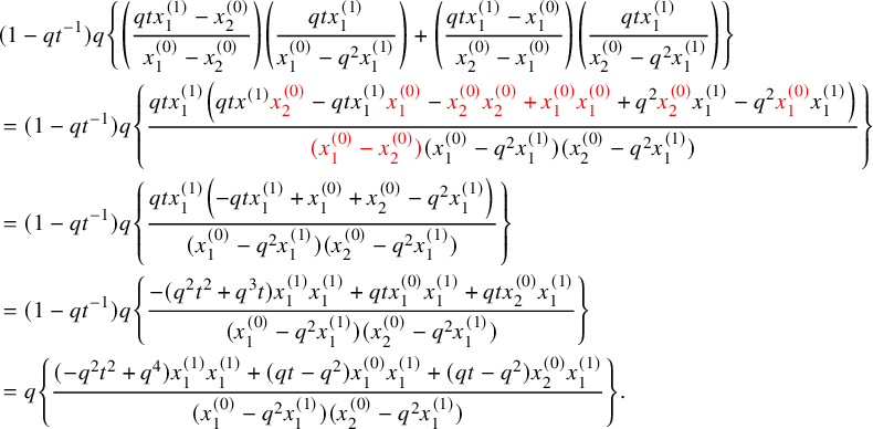
However, (5.38) becomes
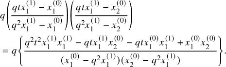 $$ \begin{align} \nonumber &q\left(\frac{qtx_1^{(1)}-x_1^{(0)}}{q^2x_1^{(1)}-x_1^{(0)}}\right)\left(\frac{qtx_1^{(1)}-x_2^{(0)}}{q^2x_1^{(1)}-x_2^{(0)}}\right)\\ &=q\left\{ \frac{q^2t^2x_1^{(1)}x_1^{(1)}-qtx_1^{(1)}x_2^{(0)}-qtx_1^{(0)}x_1^{(1)}+x_1^{(0)}x_2^{(0)}} {(x_1^{(0)}-q^2x_1^{(1)})(x_2^{(0)}-q^2x_1^{(1)})} \right\}. \end{align} $$
Combining (5.41) and (5.42) gets us
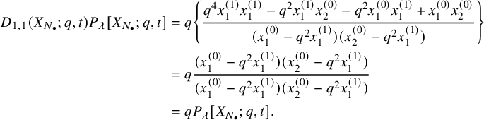 $$ \begin{align*} D_{1,1}(X_{N_{\bullet}};q,t)P_{\lambda}[X_{N_{\bullet}};q,t]&= q\left\{ \frac{q^4x_1^{(1)}x_1^{(1)}-q^2x_1^{(1)}x_2^{(0)}-q^2x_1^{(0)}x_1^{(1)}+x_1^{(0)}x_2^{(0)}} {(x_1^{(0)}-q^2x_1^{(1)})(x_2^{(0)}-q^2x_1^{(1)})} \right\}\\ &=q\frac{(x_1^{(0)}-q^2x_1^{(1)})(x_2^{(0)}-q^2x_1^{(1)})}{(x_1^{(0)}-q^2x_1^{(1)})(x_2^{(0)}-q^2x_1^{(1)})}\\ &=qP_{\lambda}[X_{N_{\bullet}};q,t]. \end{align*} $$
Example 5.14. Let $r=2$
,
$r=2$
, $p=0$
,
$p=0$
, $N_{\bullet }=(1,1)$
, and
$N_{\bullet }=(1,1)$
, and $\lambda =(1,1)$
. Here,
$\lambda =(1,1)$
. Here,
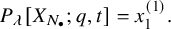 $$\begin{align*}P_{\lambda}[X_{N_{\bullet}};q,t]=x_1^{(1)}.\end{align*}$$
There are two shift patterns containing $0$
:
$0$
:
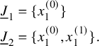 $$ \begin{align*} {\underline{J}}_1&=\{x_1^{(0)}\}\\ {\underline{J}}_2&=\{x_1^{(0)},x_1^{(1)}\}. \end{align*} $$
We then have
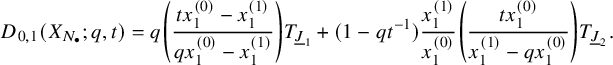 $$ \begin{align*} D_{0,1}(X_{N_{\bullet}};q,t)&= q\left( \frac{tx_1^{(0)}-x_1^{(1)}}{qx_1^{(0)}-x_1^{(1)}} \right)T_{{\underline{J}}_1} +(1-qt^{-1}) \frac{x_1^{(1)}}{x_1^{(0)}} \left( \frac{tx_1^{(0)}}{x_1^{(1)}-qx_1^{(0)}} \right)T_{{\underline{J}}_2}. \end{align*} $$
Observe that
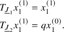 $$ \begin{align*} T_{{\underline{J}}_1}x_1^{(1)}&=x_1^{(1)}\\ T_{{\underline{J}}_2}x_1^{(1)}&=qx_1^{(0)}. \end{align*} $$
Altogether then,
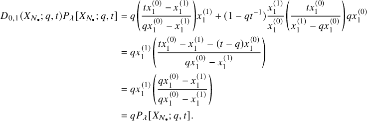 $$ \begin{align*} D_{0,1}(X_{N_{\bullet}};q,t)P_{\lambda}[X_{N_{\bullet}};q,t] &=q\left( \frac{tx_1^{(0)}-x_1^{(1)}}{qx_1^{(0)}-x_1^{(1)}} \right)x_1^{(1)} +(1-qt^{-1}) \frac{x_1^{(1)}}{x_1^{(0)}} \left( \frac{tx_1^{(0)}}{x_1^{(1)}-qx_1^{(0)}} \right)qx_1^{(0)}\\ &=qx_1^{(1)}\left(\frac{tx_1^{(0)}-x_1^{(1)}-(t-q)x_1^{(0)}}{qx_1^{(0)}-x_1^{(1)}}\right)\\ &=qx_1^{(1)}\left(\frac{qx_1^{(0)}-x_1^{(1)}}{qx_1^{(0)}-x_1^{(1)}}\right)\\ &=qP_{\lambda}[X_{N_{\bullet}};q,t]. \end{align*} $$
5.3 Higher degree operators
Now we consider higher values of n. The order n wreath Macdonald operators are defined as follows:
 $$ \begin{align} D_{p,n}^*(X_{N_{\bullet}};q,t^{-1}) &:=\frac{(-1)^{\frac{n(n-1)}{2}}}{\prod_{k=1}^n(1-q^{-k}t^{-k})}\\&\times \sum_{\mathbf{{\underline{J}}}\in Sh_p^{[n]}(X_{N_{\bullet}})} \overset{\curvearrowright}{\prod_{a=1}^n} \left\{(1-q^{-1}t^{-1})^{|{\underline{J}}_a|} \left(\frac{x^{(p+1)}_{{\underline{J}}_a^\vartriangle}}{x^{(0)}_{{\underline{J}}_a^\vartriangle}}\right) \frac{\displaystyle \prod_{\substack{l=1\\ x^{(p)}_{l}\not\in|\mathbf{{\underline{J}}}|_{\ge a}}}^{N_p}\left( tx^{(p+1)}_{{\underline{J}}_a^\vartriangle}-x^{(p)}_{l} \right)} {\displaystyle \prod_{\substack{l=1\\ x^{(p)}_{l}\not\in|\mathbf{{\underline{J}}}|_{\le a}}}^{N_p}\left( x^{(p)}_{{\underline{J}}_a}-x^{(p)}_{l} \right)}\right.\nonumber\\&\times \left. \left( \prod_{\substack{i\in I\\ i\not= p}}\, \prod_{\substack{l=1\\ x^{(i)}_{l}\not=x^{(i)}_{{\underline{J}}_a^\vartriangle}}}^{N_i} \frac{\left(tx^{(i+1)}_{{\underline{J}}_a^\vartriangle}-x^{(i)}_{l}\right)} {\left( x^{(i)}_{{\underline{J}}_a^\vartriangle}-x^{(i)}_{l} \right)} \right) \left( \prod_{i\in J_a\backslash \left\{ p \right\}} \frac{qt T_{{\underline{J}}_a}^{-1}(x^{(i)}_{{\underline{J}}_a})} {\left( x^{(i)}_{{\underline{J}}_a}-T_{{\underline{J}}_a}^{-1}(x^{(i)}_{{\underline{J}}_a}) \right)} \right) T_{{\underline{J}}_a}^{-1}\right\}\nonumber \end{align} $$
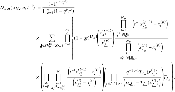 $$ \begin{align} D_{p,n}(X_{N_{\bullet}};q,t^{-1}) &:= \frac{(-1)^{\frac{n(n-1)}{2}}}{\prod_{k=1}^n(1-q^{k}t^{k})} \\&\times\sum_{\mathbf{{\underline{J}}}\in Sh_p^{[n]}(X_{N_{\bullet}})} \overset{\curvearrowright}{\prod_{a=1}^n} \left\{(1-qt)^{|{\underline{J}}_a|}\left(\frac{x^{(r-1)}_{{\underline{J}}_a^\triangledown}}{x^{(p)}_{{\underline{J}}_a}}\right) \frac{\displaystyle \prod_{\substack{l=1\\x^{(p)}_{l}\not\in|\mathbf{{\underline{J}}}|_{\ge a}}}^{N_p}\left( t^{-1}x^{(p-1)}_{{\underline{J}}_a^\triangledown}-x^{(p)}_{l} \right)} {\displaystyle \prod_{\substack{l=1\\x^{(p)}_{l}\not\in|\mathbf{{\underline{J}}}|_{\le a}}}^{N_p}\left( x^{(p)}_{{\underline{J}}_a}-x^{(p)}_{l} \right)}\right.\nonumber\\ &\times \left. \left( \prod_{\substack{i\in I\\ i\not= p}}\, \prod_{\substack{l=1\\ x^{(i)}_{l}\not=x^{(i)}_{{\underline{J}}_a^\triangledown}}}^{N_i} \frac{\left(t^{-1}x^{(i-1)}_{{\underline{J}}_a^\triangledown}-x^{(i)}_{l}\right)} {\left( x^{(i)}_{{\underline{J}}_a^\triangledown}-x^{(i)}_{l} \right)} \right) \left( \prod_{i\in J_a\backslash \left\{ p \right\}} \frac{q^{-1}t^{-1} T_{{\underline{J}}_a}(x^{(i)}_{{\underline{J}}_a})} {\left( x_{i,{\underline{J}}_a}-T_{{\underline{J}}_a}(x^{(i)}_{{\underline{J}}_a}) \right)} \right) T_{{\underline{J}}_a}\right\}.\notag\end{align} $$
Here, recall our notation for ordered products/compositions (3.12).
Remark 5.15. In contrast with the $n=1$
case, it is less obvious that these yield the higher-order Macdonald operators with t inverted when
$n=1$
case, it is less obvious that these yield the higher-order Macdonald operators with t inverted when $r=1$
. When
$r=1$
. When $r=1$
, note that our sum is over ordered n-tuples of distinct shift operators, whereas the usual formula for the nth Macdonald operator is over unordered n-tuples. Summing over the orderings for a given n-tuple, the numerator will contain a factor that is antisymmetric, while the denominator will contain a Vandermonde determinant. The quotient of these two will yield
$r=1$
, note that our sum is over ordered n-tuples of distinct shift operators, whereas the usual formula for the nth Macdonald operator is over unordered n-tuples. Summing over the orderings for a given n-tuple, the numerator will contain a factor that is antisymmetric, while the denominator will contain a Vandermonde determinant. The quotient of these two will yield $(-t)^{\pm \frac {n(n-1)}{2}}$
times the
$(-t)^{\pm \frac {n(n-1)}{2}}$
times the $(qt)^{\mp 1}$
-generating function of lengths of elements in
$(qt)^{\mp 1}$
-generating function of lengths of elements in $\mathfrak {S}_n$
. After consolidating all constants, one is indeed left with the nth Macdonald operator.
$\mathfrak {S}_n$
. After consolidating all constants, one is indeed left with the nth Macdonald operator.
Proposition 5.16. For general n, the integrals from Lemma 5.6 yield the following:
-
$(+)$
Assuming
$|x^{(i)}_{l}|<1$
and
$|q|,|t|\gg 1$
, we have for some
$$\begin{align*}\pi_{N_{\bullet}}\bigg( (\rho_{\vec{c}}^+\circ\Psi_+)(c^+_n\mathcal{E}_{p,n}^+)f\bigg) = \left(t^{-n|N_{\bullet}|}D_{p,n}^*(X_{N_{\bullet}}; q,t^{-1})+\sum_{k=0}^{n-1}c_{p,k,n}^+ D_{p,k}^*(X_{N_{\bullet}}; q,t^{-1}) \right)f\left[ X_{N_{\bullet}} \right] \end{align*}$$
$c_{p,k,n}^+\in \mathbb {C}(q,t)$
.
-
$(-)$
For
$|q|,|t|\ll 1$
, we have for some
$$\begin{align*}\pi_{N_{\bullet}}\bigg( (\rho_{\vec{c}}^-\circ\Psi_-)(c^-_n\mathcal{E}_{p,n}^-)f\bigg) =\left(t^{n|N_{\bullet}|}D_{p,n}(X_{N_{\bullet}};q,t^{-1}) +\sum_{k=0}^{n-1}c_{p,k,n}^-D_{p,k}(X_{N_{\bullet}};q,t^{-1})\right)f\left[ X_{N_{\bullet}} \right] \end{align*}$$
$c_{p,k,n}^-\in \mathbb {C}(q,t)$
.


Proof. In the ‘ $+$
’ case, we will start by integrating the p-colored variables
$+$
’ case, we will start by integrating the p-colored variables $\{w_{p,\bullet }\}$
. There are two kinds of poles inside the unit circle
$\{w_{p,\bullet }\}$
. There are two kinds of poles inside the unit circle $|w_{p,b}|=1$
:
$|w_{p,b}|=1$
:
-
(x) the poles
$\left( w_{p,b}-x_{l}^{(p)} \right)$
in (5.10) and -
(t) the poles
$\left( w_{p,b}-t^{-1}w_{p-1,a} \right)$
for
$a\le b$
in (5.12) and (5.14).


As in 5.2, we call them x- and t-poles, respectively. We note that evaluating two variables $w_{p,b}$
and
$w_{p,b}$
and $w_{p,b'}$
at the same pole will result in zero due to the factor
$w_{p,b'}$
at the same pole will result in zero due to the factor $\left(w_{p,b}-w_{p,b'}\right)$
in (5.12). Besides that, for
$\left(w_{p,b}-w_{p,b'}\right)$
in (5.12). Besides that, for $r>1$
, these residues can be evaluated independently, and we elect to do so. For the ‘
$r>1$
, these residues can be evaluated independently, and we elect to do so. For the ‘ $-$
’ case, we instead start with
$-$
’ case, we instead start with $\{w_{p+1,\bullet }\}$
, for which the relevant poles are now
$\{w_{p+1,\bullet }\}$
, for which the relevant poles are now
-
(x)
$\left( w_{p+1,a}-x_{l}^{(p)} \right)$
in (5.15) and -
(t)
$\left( w_{p+1,a}-tw_{p+2,b} \right)$
for
$a\le b$
in (5.17) and (5.18).


In 5.3.1 and 5.3.2 below, we analyze the results of the two possibilities:
-
1. integrating all
$w_{p,\bullet }$
at x-poles; -
2. the ‘mixed’ case where some
$w_{p,\bullet }$
is integrated at a t-pole.


The first case produces $D_{p,n}^*(q,t^{-1})$
and
$D_{p,n}^*(q,t^{-1})$
and $D_{p,n}(q,t^{-1})$
, whereas the second case yields a combination of lower order wreath Macdonald operators.
$D_{p,n}(q,t^{-1})$
, whereas the second case yields a combination of lower order wreath Macdonald operators.
5.3.1 Only x-poles
In both the ‘ $+$
’ and ‘
$+$
’ and ‘ $-$
’ cases, each of the n variables
$-$
’ cases, each of the n variables $\{ x_{l_a}^{(p)} \}_{a=1}^n$
will become part of a shift pattern containing p, so we set
$\{ x_{l_a}^{(p)} \}_{a=1}^n$
will become part of a shift pattern containing p, so we set $x_{{\underline {J}}_a}^{(p)}:=x_{l_a}^{(p)}$
. Furthermore, as these variables must be distinct, we have that the tuple
$x_{{\underline {J}}_a}^{(p)}:=x_{l_a}^{(p)}$
. Furthermore, as these variables must be distinct, we have that the tuple $\mathbf {{\underline {J}}}:=\left( {\underline {J}}_1,\ldots ,{\underline {J}}_n \right)$
will be p-distinct. After taking these residues, we will proceed as in 5.2.2 for a specific value of a.
$\mathbf {{\underline {J}}}:=\left( {\underline {J}}_1,\ldots ,{\underline {J}}_n \right)$
will be p-distinct. After taking these residues, we will proceed as in 5.2.2 for a specific value of a.
First consider the ‘ $+$
’ case. To see the effect of taking the residues
$+$
’ case. To see the effect of taking the residues $w_{p,b}=x_{{\underline {J}}_b}^{(p)}$
, we group together the factors
$w_{p,b}=x_{{\underline {J}}_b}^{(p)}$
, we group together the factors
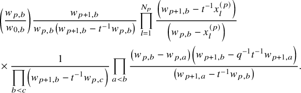 $$ \begin{align*} &\left(\frac{w_{p,b}}{w_{0,b}}\right)\frac{w_{p+1,b}}{w_{p,b}\left( w_{p+1,b}-t^{-1}w_{p,b} \right)} \prod_{l=1}^{N_p} \frac{\left( w_{p+1,b}-t^{-1}x_{l}^{(p)} \right)} {\displaystyle\left( w_{p,b}-x_{l}^{(p)} \right)}\\ &\times \frac{1} {\displaystyle \prod_{b<c} \left( w_{p+1,b}-t^{-1}w_{p,c} \right)} \prod_{a<b}\frac{ \displaystyle \left( w_{p,b}-w_{p,a} \right)\left( w_{p+1,b}-q^{-1}t^{-1}w_{p+1,a} \right)} {\left( w_{p+1,a}-t^{-1}w_{p,b} \right)}. \end{align*} $$
Upon taking residues, this becomes
 $$ \begin{align} \left(\frac{w_{p+1,b}}{w_{0,b}}\right) \frac{\displaystyle \prod_{\substack{l=1\\x_{l}^{(p)}\not\in|\mathbf{{\underline{J}}}|}}^{N_p} \left( w_{p+1,b}-t^{-1}x_{l}^{(p)} \right)} {\displaystyle \prod_{\substack{l=1\\x_{l}^{(p)}\not\in|\mathbf{{\underline{J}}}|_{\le b}}}^{N_p} \left( x_{{\underline{J}}_b}^{(p)}-x_{l}^{(p)} \right)} \underbrace{\prod_{a<b}\left( w_{p+1,b}-q^{-1}t^{-1}w_{p+1,a} \right)}_{(\dagger)}. \end{align} $$
The next variable we consider is $w_{p+1,1}$
. Notice that we have canceled the poles
$w_{p+1,1}$
. Notice that we have canceled the poles $\left( w_{p+1,1}-t^{-1}w_{p,b} \right)$
for all
$\left( w_{p+1,1}-t^{-1}w_{p,b} \right)$
for all $b\ge 1$
, and consequently, the only two kinds of poles within the unit circle
$b\ge 1$
, and consequently, the only two kinds of poles within the unit circle $|w_{p+1,1}|=1$
are as before in 5.2.2. We group together the factors
$|w_{p+1,1}|=1$
are as before in 5.2.2. We group together the factors
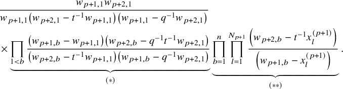 $$ \begin{align*} &\frac{w_{p+1,1}w_{p+2,1}} {w_{p+1,1}\left( w_{p+2,1}-t^{-1}w_{p+1,1} \right)\left( w_{p+1,1}-q^{-1}w_{p+2,1} \right)}\\ &\times \underbrace{\prod_{1<b} \frac{ \left( w_{p+1,b}-w_{p+1,1} \right)\left(w_{p+2,b}-q^{-1}t^{-1}w_{p+2,1} \right)} {\left( w_{p+2,b}-t^{-1}w_{p+1,1} \right)\left( w_{p+1,b}-q^{-1}w_{p+2,1} \right)}}_{(*)} \underbrace{\prod_{b=1}^n\prod_{l=1}^{N_{p+1}} \frac{\left( w_{p+2,b}-t^{-1}x_{l}^{(p+1)} \right)} {\left( w_{p+1,b}-x_{l}^{(p+1)} \right)}}_{(**)}. \end{align*} $$
The residues are
-
1. Residue at
$w_{p+1,1}=q^{-1}w_{p+2,1}$
: In this case, the factors in
$(*)$
cancel out, leaving behind
$$\begin{align*}\frac{1}{(1-q^{-1}t^{-1})} \left.\prod_{b=1}^n\prod_{l=1}^{N_{p+1}} \frac{\left( w_{p+2,b}-t^{-1}x_{l}^{(p+1)} \right)} {\left( w_{p+1,b}-x_{l}^{(p+1)} \right)}\right|_{w_{p+1,1}\mapsto q^{-1}w_{p+2,1}}. \end{align*}$$
As in 5.2.2,
$w_{p+1,1}$
will ultimately be evaluated at
$x^{(p+1)}_{{\underline {J}}_1^\vartriangle }$
, and the poles above lie outside the unit circle
$|w_{p+2,1}|=1$
because
$|q|\gg 1$
. -
2. Residue at
$w_{p+1,1}=x_{l}^{(p+1)}=:x^{(p+1)}_{{\underline {J}}_1}$
: Here, the factors in
$(*)$
cancel with those in
$(**)$
containing
$x^{(p+1)}_{{\underline {J}}_1}$
. We are left with (5.46)
$$ \begin{align} \nonumber&\frac{w_{p+2,1}}{\left( x^{(p+1)}_{{\underline{J}}_1}-q^{-1}w_{p+2,1} \right)} \prod_{\substack{l=1\\x^{(p+1)}_{l}\not=x^{(p+1)}_{{\underline{J}}_1}}}^{N_{p+1}} \frac{\left( w_{p+2,1}-t^{-1}x^{(p+1)}_{l} \right)} {\left( x_{p+1,{\underline{J}}_1}-x^{(p+1)}_{l} \right)}\\ &\times\prod_{1<b} \left\{\frac{\left( w_{p+2,b}-q^{-1}t^{-1}w_{p+2,1} \right)} {\left( w_{p+1,b}-q^{-1}w_{p+2,1} \right)} \prod_{\substack{l=1\\x^{(p+1)}_{l}\not=x^{(p+1)}_{{\underline{J}}_1}}}^{N_{p+1}} \frac{\left( w_{p+2,b}-t^{-1}x^{(p+1)}_{l} \right)} {\left(w_{p+1,b}-x^{(p+1)}_{l}\right)}\right\}. \end{align} $$
Because
$|q|\gg 1$
, the pole
$\left( x^{(p+1)}_{{\underline {J}}_1}-q^{-1}w_{p+2,1} \right)$
lies outside the unit circle
$|w_{p+2,1}|=1$
. Our key organizational trick here is that when
$w_{p+2,1}$
is ultimately evaluated at
$x^{(p+2)}_{{\underline {J}}_1^\vartriangle }$
, then we can use (5.23) to write (5.46) as since
$$\begin{align*}T_{{\underline{J}}_1}^{-1}\left( \prod_{1<b}^n\prod_{l=1}^{N_{p+1}} \frac{\left( w_{p+2,b}-t^{-1}x^{(p+1)}_{l} \right)} {\left( w_{p+1,b}-x^{(p+1)}_{l} \right)} \right) \end{align*}$$
$T_{{\underline {J}}_1}$
will only affect
$x^{(p+1)}_{{\underline {J}}_1}$
.


This pattern continues upwards in cyclic order for the variables $w_{i,1}$
. The x-variables where we take residues give a shift pattern
$w_{i,1}$
. The x-variables where we take residues give a shift pattern ${\underline {J}}_1$
containing p, and
${\underline {J}}_1$
containing p, and $w_{i,1}$
is evaluated at
$w_{i,1}$
is evaluated at $x^{(i)}_{{\underline {J}}_1^\vartriangle }$
. In (5.45), the term in
$x^{(i)}_{{\underline {J}}_1^\vartriangle }$
. In (5.45), the term in $(\dagger )$
for
$(\dagger )$
for $a=1$
can be rewritten as
$a=1$
can be rewritten as $\left( w_{p+1,b}-t^{-1}T_{{\underline {J}}_1}^{-1}x^{(p)}_{{\underline {J}}_1} \right)$
. Finally, we note that by Lemma 5.8, these residues result in
$\left( w_{p+1,b}-t^{-1}T_{{\underline {J}}_1}^{-1}x^{(p)}_{{\underline {J}}_1} \right)$
. Finally, we note that by Lemma 5.8, these residues result in $T_{{\underline {J}}_1}^{-1}$
applied to
$T_{{\underline {J}}_1}^{-1}$
applied to $f\left[ X_{N_{\bullet }} \right]$
. Thus, we can rewrite the result after taking the residues for
$f\left[ X_{N_{\bullet }} \right]$
. Thus, we can rewrite the result after taking the residues for $a=1$
as
$a=1$
as
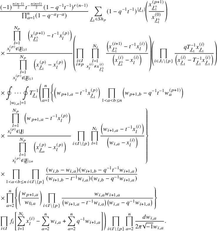 $$ \begin{align*} &\frac{(-1)^{\frac{n(n-1)}{2}}t^{-\frac{n(n+1)}{2}}(1-q^{-1}t^{-1})^{r(n-1)}}{\prod_{a=1}^n(1-q^{-a}t^{-a})} \sum_{{\underline{J}}_1\in Sh_p}(1-q^{-1}t^{-1})^{|{\underline{J}}_1|}\left(\frac{x^{(p+1)}_{{\underline{J}}_1^\vartriangle}}{x^{(0)}_{{\underline{J}}_1^\vartriangle}}\right) \\ &\times \frac{\displaystyle \prod_{\substack{l=1\\x^{(p)}_{l}\not\in|\mathbf{{\underline{J}}}|_{\ge 1}}}^{N_p}\left( x^{(p+1)}_{{\underline{J}}_1^\vartriangle}-t^{-1}x^{(p)}_{l} \right)} {\displaystyle \prod_{\substack{l=1\\x^{(p)}_{l}\not\in|\mathbf{{\underline{J}}}|_{\le 1}}}^{N_p}\left( x^{(p)}_{{\underline{J}}_1}-x^{(p)}_{l} \right)} \left( \prod_{\substack{i\in I\\i\not= p}}\, \prod_{\substack{l=1\\x^{(i)}_{l}\not=x^{(i)}_{{\underline{J}}_1^\vartriangle}}}^{N_i}\frac{\left(x^{(i+1)}_{{\underline{J}}_1^\vartriangle}-t^{-1}x^{(i)}_{l}\right)} {\left( x^{(i)}_{{\underline{J}}_1^\vartriangle}-x^{(i)}_{l} \right)} \right) \left( \prod_{i\in J_1\backslash \left\{ p \right\}} \frac{q T_{{\underline{J}}_1}^{-1}x^{(i)}_{{\underline{J}}_1}} {\left( x^{(i)}_{{\underline{J}}_1}-T_{{\underline{J}}_1}^{-1}x^{(i)}_{{\underline{J}}_1} \right)} \right)\\&\times \underset{|w_{i,a}|=1}{\oint\cdots\oint} T_{{\underline{J}}_1}^{-1}\left( \prod_{a=1}^{n}\left\{ \left( w_{p+1,a}-t^{-1}x^{(p)}_{{\underline{J}}_1} \right) \prod_{1< a<b\le n} \left( w_{p+1,b}-q^{-1}t^{-1}w^{(p+1)}_{a} \right) \right.\right.\\ &\times \left. \frac{\displaystyle \prod_{\substack{l=1\\ x^{(p)}_{l}\not\in|\mathbf{{\underline{J}}}|}}^{N_p}\left( w_{p+1,a}-t^{-1}x^{(p)}_{l} \right)} {\displaystyle \prod^{N_p}_{\substack{l=1\\x^{(p)}_{l}\not\in |\mathbf{{\underline{J}}}|_{\le a}}}\left( x^{(p)}_{{\underline{J}}_a}-x^{(p)}_{l} \right)} \prod_{i\in I\backslash\left\{ p \right\}}\prod_{l=1}^{N_{i}} \frac{\displaystyle \left( w_{i+1,a}-t^{-1}x^{(i)}_{l} \right)}{\displaystyle\left( w_{i,a}-x^{(i)}_{l} \right)}\right\}\\ &\times\prod_{1< a<b\le n} \prod_{i\in I\backslash\{p\}} \frac{(w_{i,b}-w_{i,a})(w_{i+1,b}-q^{-1}t^{-1}w_{i+1,a})}{(w_{i+1,b}-t^{-1}w_{i,a})(w_{i,b}-q^{-1}w_{i+1,a})}\\ &\times\prod_{a=2}^{n} \left\{ \left(\frac{w_{p+1,a}}{w_{0,a}}\right) \prod_{i\in I\setminus\{p\}} \frac{w_{i,a}w_{i+1,a}}{\left(w_{i+1,a}-t^{-1}w_{i,a}\right)\left(w_{i,a}-q^{-1}w_{i+1,a}\right)} \right\}\\ &\left. \prod_{i\in I}f_i\left[ \sum_{l=1}^{N_i}x_{l}^{(i)}-\sum_{a=2}^n w_{i, a}+\sum_{a=2}^nq^{-1} w_{i+1,a} \right]\right)\prod_{i\in I\backslash\{p\}}\prod_{a=2}^n\frac{dw_{i,a}}{2\pi\sqrt{-1}w_{i,a}}. \end{align*} $$
We have written this so that we can repeat the calculation for $a=1$
for general a in increasing order. Note that as we do this, we can rewrite factors in
$a=1$
for general a in increasing order. Note that as we do this, we can rewrite factors in $(\dagger )$
of (5.45) in terms of
$(\dagger )$
of (5.45) in terms of $T_{{\underline {J}}_a}^{-1}x_{p,{\underline {J}}_a}$
using (5.23). The end result of the residue calculation is
$T_{{\underline {J}}_a}^{-1}x_{p,{\underline {J}}_a}$
using (5.23). The end result of the residue calculation is
 $$\begin{align*}t^{-n|N_{\bullet}|}D_{p,n}^*(X_{N_{\bullet}}; q,t^{-1})f\left[ X_{N_{\bullet}} \right].\end{align*}$$
The ‘ $-$
’ case is similar. We begin by taking residues of
$-$
’ case is similar. We begin by taking residues of $\{w_{p+1,\bullet }\}$
and then start instead at
$\{w_{p+1,\bullet }\}$
and then start instead at $x^{(p)}_{n}$
. Afterwards, we continue downwards in cyclic order until we have taken constant terms of all variables with
$x^{(p)}_{n}$
. Afterwards, we continue downwards in cyclic order until we have taken constant terms of all variables with $a=n$
. We then continue downwards in a. The end result is then
$a=n$
. We then continue downwards in a. The end result is then
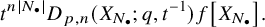 $$\begin{align*}t^{n|N_{\bullet}|}D_{p,n}(X_{N_{\bullet}};q,t^{-1})f\left[ X_{N_{\bullet}} \right]. \end{align*}$$
5.3.2 Mixed poles
In the case where there are t-poles, our goal is to show that the result is a linear combination of the lower order operators applied to $f\left[ X_{N_{\bullet }} \right]$
:
$f\left[ X_{N_{\bullet }} \right]$
: $D_{p,k}^*(X_{N_{\bullet }}; q,t^{-1})$
in the ‘
$D_{p,k}^*(X_{N_{\bullet }}; q,t^{-1})$
in the ‘ $+$
’ case and
$+$
’ case and $D_{p,k}(X_{N_{\bullet }}; q,t^{-1})$
in the ‘
$D_{p,k}(X_{N_{\bullet }}; q,t^{-1})$
in the ‘ $-$
’ case, where
$-$
’ case, where $k<n$
. Unlike in the case of
$k<n$
. Unlike in the case of $n=1$
, we will not try to compute the coefficients of this linear combination – we will compute them indirectly in 5.4. As in all the previous cases, the initial residues force a string of other residues, and we will first compute these strings that start from the initial t-poles. Once these variables are evaluated, the remaining terms will evaluate like 5.3.1.
$n=1$
, we will not try to compute the coefficients of this linear combination – we will compute them indirectly in 5.4. As in all the previous cases, the initial residues force a string of other residues, and we will first compute these strings that start from the initial t-poles. Once these variables are evaluated, the remaining terms will evaluate like 5.3.1.
In the ‘ $+$
’ case, let
$+$
’ case, let $1\le b_1^p\le n$
be any index where the residue for
$1\le b_1^p\le n$
be any index where the residue for $w_{p, b_{1}^p}$
is taken at a t-pole. Denote this pole by
$w_{p, b_{1}^p}$
is taken at a t-pole. Denote this pole by $w_{p,b_1^p}=t^{-1}w_{p-1,b_1^{p-1}}$
. In contrast to our previous calculations, we will not always cancel out factors but rather remark on why taking residues at certain poles will result in zero. The poles contributing within the unit circle
$w_{p,b_1^p}=t^{-1}w_{p-1,b_1^{p-1}}$
. In contrast to our previous calculations, we will not always cancel out factors but rather remark on why taking residues at certain poles will result in zero. The poles contributing within the unit circle $|w_{p-1,b_1^{p-1}}|=1$
are as follows.
$|w_{p-1,b_1^{p-1}}|=1$
are as follows.
-
1.
$(w_{p-1,b_1^{p-1}}-q^{-1}w_{p,a} )$
for
$a\ge b_1^{p-1}$
: If
$a<b_1^p$
, then the factor
$( w_{p,b_1^p}-q^{-1}t^{-1}w_{p,a } )$
in the numerator of (5.12) becomes zero when taking this residue. If
$a=b_1^{p-1}=b_1^p$
, then this is a pole at
$0$
, which cancels with the extra factor of
$w_{p-1,b_1^{p-1}}$
as in 5.2.1. -
2.
$( w_{p-1,b_1^{p-1}}-x^{(p-1)}_{l} )$
: The factor
$( w_{p,b_1^p}-t^{-1}x^{(p-1)}_{l} )$
in the numerator of (5.10) will evaluate to zero. -
3.
$( w_{p-1,b_1^{p-1}}-t^{-1}w_{p-2,a} )$
for
$a\le b_1^{p-1}$
: These poles possibly yield nonzero residues.


Taking a residue of the third kind, we evaluate $w_{p-1,b_1^{p-1}}=t^{-1}w_{p-2,b_1^{p-2}}$
for some
$w_{p-1,b_1^{p-1}}=t^{-1}w_{p-2,b_1^{p-2}}$
for some $b_1^{p-2}\le b_1^{p-1}$
.
$b_1^{p-2}\le b_1^{p-1}$
.
This pattern continues downwards in cyclic order, picking out variables $w_{i, b_1^i}$
where
$w_{i, b_1^i}$
where $b_1^p\ge b_1^{p-1}\ge \cdots \ge b_1^{p+1}$
. At
$b_1^p\ge b_1^{p-1}\ge \cdots \ge b_1^{p+1}$
. At $w_{p+1,b_1^{p+1}}$
, the pole of type (3) becomes
$w_{p+1,b_1^{p+1}}$
, the pole of type (3) becomes
-
(3’)
$(w_{p+1,b_1^{p+1}}-t^{-1}w_{p,a})$
for all a: If
$w_{p,a}$
is evaluated at an x-variable
$x^{(p)}_{l}$
, then as in 5.3.1, the factor
$(w_{p+1,b_1^{p+1}}-t^{-1}x^{(p)}_{l})$
will evaluate to zero upon taking this residue. Thus, only the case where
$w_{p,a}$
is evaluated at a t-pole yields a nonzero residue. For
$a=b_1^p$
, this is a pole at
$w_{p+1,b_1^{p+1}}=0$
. If
$b_{1}^{p+2}=b_1^{p+1}$
, then because of the analogue of case (1), there are no extra powers of
$w_{p+1,b_1^{p+1}}$
to cancel this pole.


If we take the residue in (3’) at $w_{p,a}$
evaluated at a t-pole but
$w_{p,a}$
evaluated at a t-pole but $a\not =b_1^p$
, then we set
$a\not =b_1^p$
, then we set $b_2^p:=a$
. Letting the t-pole be
$b_2^p:=a$
. Letting the t-pole be $(w_{p,b_2^p}-t^{-1}w_{p-1,b_2^{p-1}})$
for
$(w_{p,b_2^p}-t^{-1}w_{p-1,b_2^{p-1}})$
for $b_2^{p-1}\le b_2^p$
, the process is similar to as before. There is just one alteration to the poles of type (3):
$b_2^{p-1}\le b_2^p$
, the process is similar to as before. There is just one alteration to the poles of type (3):
-
(3”)
$(w_{i, b_2^{i}}-t^{-1}w_{i-1,b_1^{i-1}})$
: This is a pole at
$0$
, which cancels with the factor
$\pm (w_{i, b_2^i}- w_{i, b_1^i})$
in the numerator of (5.11).


Thus, we avoid variables that we have already evaluated. Note that at first glance, the product of factors in (5.11) and (5.12) involving $w_{i, b_2^i}$
and
$w_{i, b_2^i}$
and $w_{j,b_1^j}$
may contribute a pole at
$w_{j,b_1^j}$
may contribute a pole at $0$
, but in fact, their products have total degree zero and thus become a constant. There is an outlier case of
$0$
, but in fact, their products have total degree zero and thus become a constant. There is an outlier case of $(w_{p+1,b_1^{p+1}}-t^{-1}w_{p,b_{2}^p})$
, which has been removed when we take residues, but this can be replaced with
$(w_{p+1,b_1^{p+1}}-t^{-1}w_{p,b_{2}^p})$
, which has been removed when we take residues, but this can be replaced with $(w_{p+1,b_1^{p+1}}-t^{-1}w_{p,b_{1}^p})$
to restore the degree zero balance. We continue like this to new indices
$(w_{p+1,b_1^{p+1}}-t^{-1}w_{p,b_{1}^p})$
to restore the degree zero balance. We continue like this to new indices $\{b_3^i\}_{i\in I}, \left\{ b_{4}^i \right\}_{i\in I},$
etc. until either there are no more nonzero residues or we finally take the residue at
$\{b_3^i\}_{i\in I}, \left\{ b_{4}^i \right\}_{i\in I},$
etc. until either there are no more nonzero residues or we finally take the residue at $0$
of
$0$
of $z_{p+1, b_k^{p+1}}$
for some final value k.
$z_{p+1, b_k^{p+1}}$
for some final value k.
For $1\le m<m'\le k$
, we note that as in the
$1\le m<m'\le k$
, we note that as in the $(m,m')=(1,2)$
case, the product of the binomials in (5.11) and (5.12) involving one variable from
$(m,m')=(1,2)$
case, the product of the binomials in (5.11) and (5.12) involving one variable from $\{w_{i,b_m^i}\}_{i\in I}$
and another variable from
$\{w_{i,b_m^i}\}_{i\in I}$
and another variable from $\{w_{j, b_{m'}^j}\}_{i\in I}$
has degree zero provided we make the same adjustment for
$\{w_{j, b_{m'}^j}\}_{i\in I}$
has degree zero provided we make the same adjustment for $i=p+1$
and
$i=p+1$
and $m'=m+1$
. Thus, these factors turn into a constant. To consider binomials involving only
$m'=m+1$
. Thus, these factors turn into a constant. To consider binomials involving only $\{w_{i,b_m^i}\}_{i\in I}$
for one value of m, we note that when we take the residues, we remove
$\{w_{i,b_m^i}\}_{i\in I}$
for one value of m, we note that when we take the residues, we remove
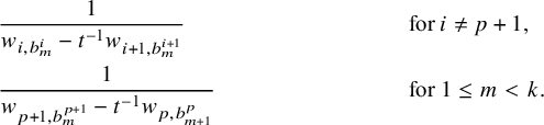 $$ \begin{align*} &\frac{1}{w_{i,b_m^i}-t^{-1}w_{i+1,b_m^{i+1}}} &&\mbox{for }i\not=p+1,\\ &\frac{1}{w_{p+1,b_m^{p+1}}-t^{-1}w_{p,b_{m+1}^{p}}} &&\mbox{for }1\le m<k. \end{align*} $$
There is a leftover power of $w_{i,b_{m}^i}$
for
$w_{i,b_{m}^i}$
for $i\not =p$
from (5.13) and (5.14), and as discussed in the pole of type (1) above, these are only absorbed when
$i\not =p$
from (5.13) and (5.14), and as discussed in the pole of type (1) above, these are only absorbed when $b_{m}^{i+1}=b_{m}^i$
. These unabsorbed powers turn the entire integral zero when we take the final residue
$b_{m}^{i+1}=b_{m}^i$
. These unabsorbed powers turn the entire integral zero when we take the final residue $w_{p+1,b_k^{p+1}}=0$
. Thus, we only need to consider the case where for each m,
$w_{p+1,b_k^{p+1}}=0$
. Thus, we only need to consider the case where for each m,
 $$\begin{align*}b_m^p=b_m^{p-1}=\cdots=b_m^{p+1}=:b_m.\end{align*}$$
In this case, all factors only involving $\{w_{i,b_m}\}_{i\in I}^{1\le m\le k}$
leave behind a constant. Evidently, the corresponding terms in (5.13) and (5.14) disappear. The terms involving
$\{w_{i,b_m}\}_{i\in I}^{1\le m\le k}$
leave behind a constant. Evidently, the corresponding terms in (5.13) and (5.14) disappear. The terms involving $w_{i,b_m}$
and an x-variable in (5.10) leave behind a power of t when we cancel
$w_{i,b_m}$
and an x-variable in (5.10) leave behind a power of t when we cancel
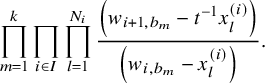 $$\begin{align*}\prod_{m=1}^k\prod_{i\in I}\prod_{l=1}^{N_i}\frac{\left( w_{i+1,b_{m}}-t^{-1}x^{(i)}_{l} \right)} {\left( w_{i,b_{m}}-x^{(i)}_{l} \right)}. \end{align*}$$
Finally, the product of terms in (5.11) involving any index $1\le a\le n$
and
$1\le a\le n$
and $b_m$
leave behind a constant when we evaluate
$b_m$
leave behind a constant when we evaluate $w_{i,b_m}=0$
for all
$w_{i,b_m}=0$
for all $i\in I$
. The remaining factors are a scalar multiple of the calculation for
$i\in I$
. The remaining factors are a scalar multiple of the calculation for $\mathcal {E}_{p,n-k}$
. The ‘
$\mathcal {E}_{p,n-k}$
. The ‘ $-$
’ case is analyzed similarly.
$-$
’ case is analyzed similarly.
5.4 Eigenvalues
To describe the eigenvalues of the operators (5.43) and (5.44), we will use the elementary symmetric functions $ e_k$
. As in the proof of Theorem 5.11, Proposition 5.16 gives us the following:
$ e_k$
. As in the proof of Theorem 5.11, Proposition 5.16 gives us the following:
Proposition 5.17. Recall the coefficients $\{c_{p,k,n}^{\pm }\}$
from Proposition 5.16. We have
$\{c_{p,k,n}^{\pm }\}$
from Proposition 5.16. We have
 $$ \begin{align} \begin{aligned} &\left(t^{-n|N_{\bullet}|}D_{p,n}^*(X_{N_{\bullet}}; q,t^{-1})+\sum_{k=0}^{n-1}c_{p,k,n}^+ D_{p,k}^*(X_{N_{\bullet}}; q,t^{-1}) \right)P_{\lambda}[X_{N_{\bullet}};q,t]\\ &= e_n\left[\sum_{\substack{b=1\\b-\lambda_b\equiv p+1}}^\infty q^{-\lambda_b}t^{-b}\right]P_{\lambda}[X_{N_{\bullet}};q,t^{-1}] \end{aligned} \end{align} $$
for $|x^{(i)}_{l}|<1$
,
$|x^{(i)}_{l}|<1$
, $|q|\gg 1$
, and
$|q|\gg 1$
, and $|t|\gg 1$
and
$|t|\gg 1$
and
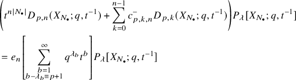 $$ \begin{align} \begin{aligned} &\left(t^{n|N_{\bullet}|}D_{p,n}(X_{N_{\bullet}};q,t^{-1}) +\sum_{k=0}^{n-1}c_{p,k,n}^-D_{p,k}(X_{N_{\bullet}};q,t^{-1})\right)P_{\lambda}[X_{N_{\bullet}};q,t^{-1}]\\ &= e_n\left[\sum_{\substack{b=1\\b-\lambda_b\equiv p+1}}^\infty q^{\lambda_b} t^{b}\right]P_{\lambda}[X_{N_{\bullet}};q,t^{-1}] \end{aligned} \end{align} $$
for $|x^{(i)}_{l}|<1$
,
$|x^{(i)}_{l}|<1$
, $|q|\ll 1$
, and
$|q|\ll 1$
, and $|t|\ll 1$
.
$|t|\ll 1$
.
Corollary 5.18. For variables and parameters satisfying the conditions in Proposition 5.17, the operators $D_{p,n}(q,t)$
and
$D_{p,n}(q,t)$
and $D_{p,n}^*(q,t)$
act diagonally on
$D_{p,n}^*(q,t)$
act diagonally on $\left\{ P_{\lambda }\left[ X_{N_{\bullet }};q,t \right] \right\}$
.
$\left\{ P_{\lambda }\left[ X_{N_{\bullet }};q,t \right] \right\}$
.
Proof. Using induction starting with the case $n=1$
from Theorem 5.11, we can use the equations in Proposition 5.17 to show that
$n=1$
from Theorem 5.11, we can use the equations in Proposition 5.17 to show that $D_{p,n}(X_{N_{\bullet }};q,t)$
and
$D_{p,n}(X_{N_{\bullet }};q,t)$
and $D_{p,n}^*(X_{N_{\bullet }};q,t)$
act diagonally on
$D_{p,n}^*(X_{N_{\bullet }};q,t)$
act diagonally on $P_{\lambda }[X_{N_{\bullet }};q,t]$
under the appropriate conditions on variables and parameters.
$P_{\lambda }[X_{N_{\bullet }};q,t]$
under the appropriate conditions on variables and parameters.
Our goal in this subsection is to extract the eigenvalues from (5.47) and (5.48) and extend their validity to generic values.
5.4.1 Spectral variables
Letting $\lambda $
vary over partitions with
$\lambda $
vary over partitions with $\mathrm {core}(\lambda )$
compatible with
$\mathrm {core}(\lambda )$
compatible with $N_{\bullet }$
and
$N_{\bullet }$
and $\ell (\lambda )\le |N_{\bullet }|$
, we note that by Proposition 2.7, the stabilized eigenvalues
$\ell (\lambda )\le |N_{\bullet }|$
, we note that by Proposition 2.7, the stabilized eigenvalues
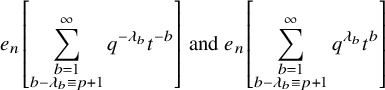 $$\begin{align*}e_n\left[\sum_{\substack{b=1\\b-\lambda_b\equiv p+1}}^\infty q^{-\lambda_b}t^{-b}\right] \mbox{ and } e_n\left[\sum_{\substack{b=1\\b-\lambda_b\equiv p+1}}^\infty q^{\lambda_b} t^{b}\right] \end{align*}$$
depend only on the $N_p$
values of b, where
$N_p$
values of b, where $1\le b\le |N_{\bullet }|$
and
$1\le b\le |N_{\bullet }|$
and $b-\lambda _b=p+1$
. We define the color p spectral variables
$b-\lambda _b=p+1$
. We define the color p spectral variables $\{ s^{(p)}_{ a} \}_{a=1}^{N_p}$
by setting
$\{ s^{(p)}_{ a} \}_{a=1}^{N_p}$
by setting
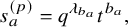 $$\begin{align*}s^{(p)}_{a}=q^{\lambda_{b_a}}t^{b_a}, \end{align*}$$
where $1\le b_a\le |N_{\bullet }|$
is the ath number where
$1\le b_a\le |N_{\bullet }|$
is the ath number where $b_a-\lambda _{b_a}\equiv p+1$
. Using these variables, we can rewrite
$b_a-\lambda _{b_a}\equiv p+1$
. Using these variables, we can rewrite
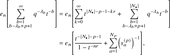 $$ \begin{align*} e_n\left[\sum_{\substack{b=1\\b-\lambda_b\equiv p+1}}^\infty q^{-\lambda_b}t^{-b}\right] &=e_n\left[\sum_{k=0}^{\infty}t^{|N_{\bullet}|-p-1-kr}+\sum_{\substack{b=1\\b-\lambda_b\equiv p+1}}^{|N_{\bullet}|} q^{-\lambda_b}t^{-b}\right]\\ &=e_n\left[\frac{t^{-|N_{\bullet}|-p-1}}{1-t^{-nr}}+\sum_{a=1}^{N_p}\left(s^{(p)}_{a}\right)^{-1} \right], \end{align*} $$
where $|t|\gg 1$
. Here, we have split off the parts above row
$|t|\gg 1$
. Here, we have split off the parts above row $|N_{\bullet }|$
as in (5.37). Similarly,
$|N_{\bullet }|$
as in (5.37). Similarly,
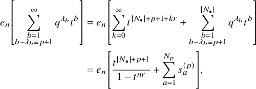 $$ \begin{align*} e_n\left[\sum_{\substack{b=1\\b-\lambda_b\equiv p+1}}^\infty q^{\lambda_b} t^{b}\right] &=e_n\left[\sum_{k=0}^\infty t^{|N_{\bullet}|+p+1+kr}+\sum_{\substack{b=1\\b-\lambda_b\equiv p+1}}^{|N_{\bullet}|} q^{\lambda_b} t^{b}\right]\\ &=e_n\left[ \frac{t^{|N_{\bullet}|+p+1}}{1-t^{nr}}+\sum_{a=1}^{N_p}s^{(p)}_{a} \right], \end{align*} $$
where $|t|\ll 1$
. The following is but a slight alteration of Lemma 3.2 from [Reference Feigin, Hashizume, Hoshino, Shiraishi and Yanagida4]:
$|t|\ll 1$
. The following is but a slight alteration of Lemma 3.2 from [Reference Feigin, Hashizume, Hoshino, Shiraishi and Yanagida4]:
Lemma 5.19. For $|t|\gg 1$
, we have
$|t|\gg 1$
, we have
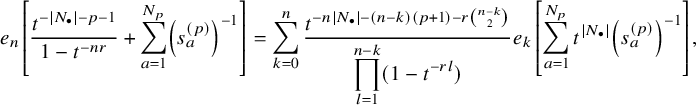 $$ \begin{align} e_n\left[\frac{t^{-|N_{\bullet}|-p-1}}{1-t^{-nr}}+\sum_{a=1}^{N_p}\left(s^{(p)}_{a}\right)^{-1} \right]=\sum_{k=0}^n\frac{t^{-n|N_{\bullet}|-(n-k)(p+1)-r\binom{n-k}{2}}}{\displaystyle\prod_{l=1}^{n-k}(1-t^{-rl})} e_k\left[ \sum_{a=1}^{N_p}t^{|N_{\bullet}|}\left(s^{(p)}_{a}\right)^{-1} \right], \end{align} $$
while for $|t|\ll 1$
, we have
$|t|\ll 1$
, we have
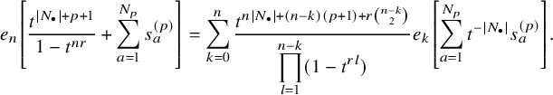 $$ \begin{align} e_n\left[\frac{t^{|N_{\bullet}|+p+1}}{1-t^{nr}}+\sum_{a=1}^{N_p}s^{(p)}_{a} \right]=\sum_{k=0}^n\frac{t^{n|N_{\bullet}|+(n-k)(p+1)+r\binom{n-k}{2}}}{\displaystyle\prod_{l=1}^{n-k}(1-t^{rl})} e_k\left[ \sum_{a=1}^{N_p}t^{-|N_{\bullet}|}s^{(p)}_{a} \right]. \end{align} $$
Proof. The basic observation is that for two alphabets X and Y and an auxilliary variable u,
 $$ \begin{align*} \sum_{n=0}^\infty e_n[X+Y]u^n &=\exp\left(-\sum_{k>0} p_k[X+Y] \frac{(-u)^k}{k}\right)\\ &=\exp\left(-\sum_{k>0} p_k[X] \frac{(-u)^k}{k}\right)\exp\left(-\sum_{k>0} p_k[Y] \frac{(-u)^k}{k}\right)\\ &=\left(\sum_{n=0}^\infty e_n[X]u^n\right)\left(\sum_{n=0}^\infty e_n[Y]u^n\right)\\ &=\sum_{n=0}^\infty\sum_{k=0}^ne_{n-k}[X]e_k[Y] u^n. \end{align*} $$
Comparing the coefficients of $u^n$
, we thus have
$u^n$
, we thus have
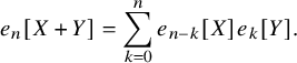 $$ \begin{align} e_n[X+Y]=\sum_{k=0}^n e_{n-k}[X]e_{k}[Y]. \end{align} $$
For (5.49), we take (5.51) and set
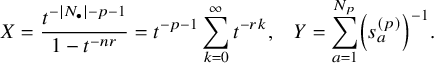 $$ \begin{align*} \begin{aligned} X&=\frac{t^{-|N_{\bullet}|-p-1}}{1-t^{-nr}}=t^{-p-1}\sum_{k=0}^\infty t^{-rk},& Y&=\sum_{a=1}^{N_p}\left(s_a^{(p)}\right)^{-1}. \end{aligned} \end{align*} $$
By the quantum binomial theorem (cf. [Reference Macdonald9, Example I.2.5]), we have
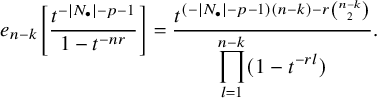 $$\begin{align*}e_{n-k}\left[\frac{t^{-|N_{\bullet}|-p-1}}{1-t^{-nr}}\right]= \frac{t^{(-|N_{\bullet}|-p-1)(n-k)-r\binom{n-k}{2}}}{\displaystyle\prod_{l=1}^{n-k}(1-t^{-rl})}. \end{align*}$$
To obtain (5.49), we break off $t^{k|N_{\bullet }|}$
and place it inside
$t^{k|N_{\bullet }|}$
and place it inside $e_k\left[\sum (s_a^{(p)})^{-1}\right]$
. The proof of (5.50) is similar.
$e_k\left[\sum (s_a^{(p)})^{-1}\right]$
. The proof of (5.50) is similar.
5.4.2 Spectral shift
By Lemma 5.19, the stabilized eigenvalues are polynomial in the spectral variables. Moreover, its degree k part is given by $e_k$
evaluated at
$e_k$
evaluated at $\{t^{-|N_{\bullet }|}s^{(p)}_{\bullet }\}$
. We would like to show that the summations in (5.47) and (5.48) correspond in some sense to this decomposition by the degree. The degree of a homogeneous polynomial can be measured using q-shifts. However, by the definition of the spectral variables, multiplying
$\{t^{-|N_{\bullet }|}s^{(p)}_{\bullet }\}$
. We would like to show that the summations in (5.47) and (5.48) correspond in some sense to this decomposition by the degree. The degree of a homogeneous polynomial can be measured using q-shifts. However, by the definition of the spectral variables, multiplying $s^{(p)}_{a}$
by q corresponds to adding a node to the end of a row. However, we must do this in a way that is color-insensitive. This motivates the following:
$s^{(p)}_{a}$
by q corresponds to adding a node to the end of a row. However, we must do this in a way that is color-insensitive. This motivates the following:
Proposition 5.20. Let $\lambda $
be a partition with core
$\lambda $
be a partition with core $\kappa (\lambda )$
compatible with
$\kappa (\lambda )$
compatible with $N_{\bullet }$
and
$N_{\bullet }$
and $\ell (\lambda )\le |N_{\bullet }|$
. Then
$\ell (\lambda )\le |N_{\bullet }|$
. Then
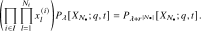 $$\begin{align*}\left(\prod_{i\in I}\prod_{l=1}^{N_i}x^{(i)}_{l}\right)P_{\lambda}[X_{N_{\bullet}}; q,t]=P_{\lambda+r^{|N_{\bullet}|}}[X_{N_{\bullet}};q,t]. \end{align*}$$
Here, $\lambda +r^{|N_{\bullet }|}$
denotes the partition obtained by adding r boxes to the first
$\lambda +r^{|N_{\bullet }|}$
denotes the partition obtained by adding r boxes to the first $|N_{\bullet }|$
rows of
$|N_{\bullet }|$
rows of $\lambda $
.
$\lambda $
.
Proof. By Corollary 5.12, $P_{\lambda +r^{|N_{\bullet }|}}[X_{N_{\bullet }};q,t]$
is characterized by the eigenvalue equations
$P_{\lambda +r^{|N_{\bullet }|}}[X_{N_{\bullet }};q,t]$
is characterized by the eigenvalue equations
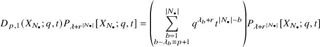 $$\begin{align*}D_{p,1}(X_{N_{\bullet}};q,t)P_{\lambda+r^{|N_{\bullet}|}}[X_{N_{\bullet}};q,t]=\left( \sum_{\substack{b=1\\ b-\lambda_b\equiv p+1}}^{|N_{\bullet}|} q^{\lambda_b+r}t^{|N_{\bullet}|-b}\right)P_{\lambda+r^{|N_{\bullet}|}}[X_{N_{\bullet}};q,t] \end{align*}$$
ranging over all $p\in I$
. Note that we have used
$p\in I$
. Note that we have used $b-\lambda _b\equiv b-\lambda _b+r$
. Now, for a shift pattern
$b-\lambda _b\equiv b-\lambda _b+r$
. Now, for a shift pattern ${\underline {J}}$
, it is easy to see that
${\underline {J}}$
, it is easy to see that
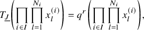 $$ \begin{align} T_{{\underline{J}}}\left(\prod_{i\in I}\prod_{l=1}^{N_i}x^{(i)}_{l}\right)=q^r\left(\prod_{i\in I}\prod_{l=1}^{N_i}x^{(i)}_{l}\right), \end{align} $$
from which the proposition follows.
5.4.3 Eigenfunction equation
We are now ready to derive the eigenvalues of the higher-order wreath Macdonald operators.
Theorem 5.21. For $\lambda $
with core
$\lambda $
with core $\kappa (\lambda )$
compatible with
$\kappa (\lambda )$
compatible with $N_{\bullet }$
according to (2.9) and
$N_{\bullet }$
according to (2.9) and $\ell (\lambda )\le |N_{\bullet }|$
, the wreath Macdonald polynomial
$\ell (\lambda )\le |N_{\bullet }|$
, the wreath Macdonald polynomial $P_{\lambda }[X_{N_{\bullet }};q,t]$
satisfies the equations
$P_{\lambda }[X_{N_{\bullet }};q,t]$
satisfies the equations
 $$ \begin{align*} D_{p,n}^*(X_{N_{\bullet}};q,t)P_{\lambda}[X_{N_{\bullet}};q,t] &= e_n\left[ \sum_{\substack{b=1\\ b-\lambda_b\equiv p+1}}^{|N_{\bullet}|}q^{-\lambda_b}t^{-|N_{\bullet}|+b} \right] P_{\lambda}[X_{N_{\bullet}};q,t]\\ D_{p,n}(X_{N_{\bullet}};q,t)P_{\lambda}[X_{N_{\bullet}};q,t] &= e_n\left[ \sum_{\substack{b=1\\ b-\lambda_b\equiv p+1}}^{|N_{\bullet}|}q^{\lambda_b}t^{|N_{\bullet}|-b} \right] P_{\lambda}[X_{N_{\bullet}};q,t]. \end{align*} $$
Here, $x_{i,l}$
, q and t take generic values.
$x_{i,l}$
, q and t take generic values.
Proof. Let $\mathfrak {e}_{p,n}(\lambda ;q,t^{-1})$
and
$\mathfrak {e}_{p,n}(\lambda ;q,t^{-1})$
and $\mathfrak {e}_{p,n}^*(\lambda ;q,t^{-1})$
be the eigenvalues of
$\mathfrak {e}_{p,n}^*(\lambda ;q,t^{-1})$
be the eigenvalues of $D_{p,n}(X_{N_{\bullet }};q,t^{-1})$
and
$D_{p,n}(X_{N_{\bullet }};q,t^{-1})$
and $D_{p,n}^*(X_{N_{\bullet }};q,t^{-1})$
, respectively, at
$D_{p,n}^*(X_{N_{\bullet }};q,t^{-1})$
, respectively, at $P_{\lambda }[X_{N_{\bullet }};q,t^{-1}]$
. Combining (5.47), (5.48), and Lemma 5.19, we have
$P_{\lambda }[X_{N_{\bullet }};q,t^{-1}]$
. Combining (5.47), (5.48), and Lemma 5.19, we have
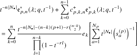 $$ \begin{align} \nonumber &t^{-n|N_{\bullet}|}\mathfrak{e}_{p,n}^*(\lambda;q,t^{-1})+\sum_{k=0}^{n-1}c_{p,k,n}^+ \mathfrak{e}_{p,k}^*(\lambda;q,t^{-1})\\ &=\sum_{k=0}^n\frac{t^{-n|N_{\bullet}|-(n-k)(p+1)-r\binom{n-k}{2}}}{\displaystyle\prod_{l=1}^{n-k}(1-t^{-rl})}e_k\left[ \sum_{a=1}^{N_p}t^{|N_{\bullet}|}\left(s^{(p)}_{a}\right)^{-1} \right] \end{align} $$
and
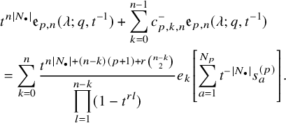 $$ \begin{align} \nonumber &t^{n|N_{\bullet}|}\mathfrak{e}_{p,n}(\lambda;q,t^{-1}) +\sum_{k=0}^{n-1}c_{p,k,n}^-\mathfrak{e}_{p,n}(\lambda;q,t^{-1})\\ &=\sum_{k=0}^n\frac{t^{n|N_{\bullet}|+(n-k)(p+1)+r\binom{n-k}{2}}}{\displaystyle\prod_{l=1}^{n-k}(1-t^{rl})}e_k\left[ \sum_{a=1}^{N_p}t^{-|N_{\bullet}|}s^{(p)}_{a} \right]. \end{align} $$
We can induct on n to show that, as functions of $\lambda $
,
$\lambda $
, $\mathfrak {e}_{p,n}(\lambda ;q,t^{-1})$
is polynomial in
$\mathfrak {e}_{p,n}(\lambda ;q,t^{-1})$
is polynomial in $\{ s_{\bullet }^{(p)} \}$
and
$\{ s_{\bullet }^{(p)} \}$
and $\mathfrak {e}_{p,n}^*(\lambda ;q,t^{-1})$
is polynomial in
$\mathfrak {e}_{p,n}^*(\lambda ;q,t^{-1})$
is polynomial in $\{ (s^{(p)}_{\bullet })^{-1} \}$
. Applying (5.52) n times, we have (when viewed as operators):
$\{ (s^{(p)}_{\bullet })^{-1} \}$
. Applying (5.52) n times, we have (when viewed as operators):
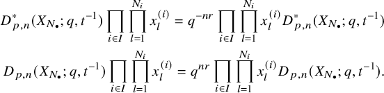 $$ \begin{align*} D_{p,n}^*(X_{N_{\bullet}};q,t^{-1})\prod_{i\in I}\prod_{l=1}^{N_i}x^{(i)}_{l}=q^{-nr}\prod_{i\in I}\prod_{l=1}^{N_i}x^{(i)}_{l}D_{p,n}^*(X_{N_{\bullet}};q,t^{-1})\\ D_{p,n}(X_{N_{\bullet}};q,t^{-1})\prod_{i\in I}\prod_{l=1}^{N_i}x^{(i)}_{l}=q^{nr}\prod_{i\in I}\prod_{l=1}^{N_i}x^{(i)}_{l}D_{p,n}(X_{N_{\bullet}};q,t^{-1}). \end{align*} $$
It then follows from Proposition 5.20 that $\mathfrak {e}_{p,n}(\lambda ;q,t^{-1})$
is homogeneous of degree n and
$\mathfrak {e}_{p,n}(\lambda ;q,t^{-1})$
is homogeneous of degree n and $\mathfrak {e}_{p,n}^*(\lambda ;q,t^{-1})$
is homogeneous of degree
$\mathfrak {e}_{p,n}^*(\lambda ;q,t^{-1})$
is homogeneous of degree $-n$
. Thus,
$-n$
. Thus, $t^{-n|N_{\bullet }|}\mathfrak {e}_{p,n}^*(\lambda ;q,t^{-1})$
is the degree
$t^{-n|N_{\bullet }|}\mathfrak {e}_{p,n}^*(\lambda ;q,t^{-1})$
is the degree $-n$
piece of (5.53) and
$-n$
piece of (5.53) and $t^{n|N_{\bullet }|}\mathfrak {e}_{p,n}(\lambda ;q,t^{-1})$
is the degree n piece of (5.54). This establishes the eigenvalue equations under the appropriate conditions (5.8) and (5.9) on
$t^{n|N_{\bullet }|}\mathfrak {e}_{p,n}(\lambda ;q,t^{-1})$
is the degree n piece of (5.54). This establishes the eigenvalue equations under the appropriate conditions (5.8) and (5.9) on $x^{(i)}_{l}$
, q and t. We extend to generic values as in the proof of Theorem 5.11.
$x^{(i)}_{l}$
, q and t. We extend to generic values as in the proof of Theorem 5.11.
Remark 5.22. Even though $r\ge 3$
was assumed throughout, we have verified experimentally that Theorem 5.21 continues to hold as stated for
$r\ge 3$
was assumed throughout, we have verified experimentally that Theorem 5.21 continues to hold as stated for $r=2$
. The
$r=2$
. The $r=1$
case is discussed in Remark 5.15 above.
$r=1$
case is discussed in Remark 5.15 above.
Example 5.23. Let $r=2$
,
$r=2$
, $p=1$
,
$p=1$
, $N_{\bullet }=(0,2)$
and
$N_{\bullet }=(0,2)$
and $\lambda =(1)$
. Because
$\lambda =(1)$
. Because $\lambda $
is a
$\lambda $
is a $2$
-core,
$2$
-core,
 $$\begin{align*}P_{\lambda}[X_{N_{\bullet}};q,t]=1. \end{align*}$$
There are only two shift patterns containing $1$
:
$1$
:
 $$ \begin{align*} {\underline{J}}_1&=\{x_1^{(1)}\}\\ {\underline{J}}_2&=\{x_2^{(1)}\}. \end{align*} $$
Note that
 $$ \begin{align*} T_{{\underline{J}}_1}x_1^{(1)}&=q^2x_1^{(1)} & T_{{\underline{J}}_2}x_1^{(1)}&=x_1^{(1)}\\ T_{{\underline{J}}_1}x_2^{(1)}&=x_1^{(1)} & T_{{\underline{J}}_2}x_2^{(1)}&=q^2x_2^{(1)}. \end{align*} $$
Therefore,
 $$ \begin{align*} D_{1,1}(X_{N_{\bullet}};q,t)P_{\lambda}[X_{\bullet};q,t]&= \frac{(-1)(1-qt^{-1})}{1-q^2t^{-2}} \left\{ \frac{qtx_2^{(1)}-q^2x_1^{(1)}}{x_1^{(1)}-x_2^{(1)}}+\frac{qtx_1^{(1)}-q^2x_2^{(1)}}{x_2^{(1)}-x_1^{(1)}} \right\}\\ &=\frac{(-1)(1-qt^{-1})(-qt-q^2)}{1-q^2t^{-2}}\\ &=qtP_{\lambda}[X_{N_{\bullet}};q,t]. \end{align*} $$
A Wreath Noumi-Sano operators
In this appendix, we apply our methods to study wreath analogues of the trigonometric Noumi-Sano operators [Reference Noumi and Sano12]. We obtain explicit formulas for degree $n=1$
and an integral formula for general n.
$n=1$
and an integral formula for general n.
A.1 Infinite-variable eigenvalues
Let $(x;y)_\infty $
denote the infinite y-Pochammer symbol:
$(x;y)_\infty $
denote the infinite y-Pochammer symbol:
 $$\begin{align*}(x;y)_\infty=\prod_{i=0}^{\infty}(1-xy^i). \end{align*}$$
Lemma A.1. Assume $|q^{\pm 1}|<1$
and
$|q^{\pm 1}|<1$
and $|t^{\pm 1}|<1$
(where ‘
$|t^{\pm 1}|<1$
(where ‘ $+$
’ and ‘
$+$
’ and ‘ $-$
’ are separate cases). For
$-$
’ are separate cases). For $p\in I$
, we have
$p\in I$
, we have
 $$ \begin{align} \begin{aligned} &\left\langle\lambda\left|\exp\left[-\sum_{k>0}\left(\frac{\sum_{i=1}^{r}q^{\pm k(i-1)}h_{p+i,\pm k}}{(1-q^{\pm kr})}\right)\frac{\mathfrak{q}^{\pm k} z^{\mp k}}{v^{\pm k}[ k]_{\mathfrak{q}}} \right]\right|\lambda\right\rangle\\ &= \exp\left[\sum_{k>0}\left(\sum_{i=1}^{r}\frac{q^{\pm k(i-1)}}{1-q^{\pm kr}}\left\{\sum_{\substack{b>0\\b-\lambda_b\equiv p+i }}q^{\pm k\lambda_b}t^{\pm kb}-t^{\mp k}\sum_{\substack{b>0\\b-\lambda_b\equiv p+i+1 }}q^{\pm k\lambda_b}t^{\pm kb}\right\}\right)\frac{z^{\mp k}}{k}\right]\\ &= \prod_{i=1}^{r} \frac{\displaystyle\prod_{\substack{b>0\\b-\lambda_b\equiv p+i+1 }}\left(q^{\pm(\lambda_b+i)}t^{\pm (b- 1)}z^{\mp 1}; q^{\pm r}\right)_\infty} {\displaystyle\prod_{\substack{b>0\\b-\lambda_b\equiv p+i }}\left(q^{\pm(\lambda_b+i)}t^{\pm b}z^{\mp 1}; q^{\pm r}\right)_\infty}, \end{aligned} \end{align} $$
where we set $\lambda _b=0$
for all
$\lambda _b=0$
for all $b>\ell (\lambda )$
.
$b>\ell (\lambda )$
.
A.2 Shuffle elements
We rewrite
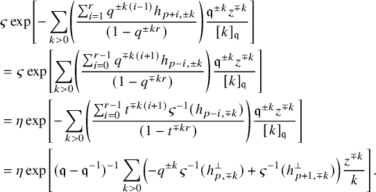 $$ \begin{align*} &\varsigma\exp\left[-\sum_{k>0}\left(\frac{\sum_{i=1}^{r}q^{\pm k(i-1)}h_{p+i,\pm k}}{(1-q^{\pm kr})}\right)\frac{\mathfrak{q}^{\pm k} z^{\mp k}}{[ k]_{\mathfrak{q}}} \right]\\ &= \varsigma\exp\left[\sum_{k>0}\left(\frac{\sum_{i=0}^{r-1}q^{\mp k(i+1)}h_{p-i,\pm k}}{(1-q^{\mp kr})}\right)\frac{\mathfrak{q}^{\pm k} z^{\mp k}}{[ k]_{\mathfrak{q}}} \right]\\ &=\eta\exp\left[-\sum_{k>0}\left(\frac{\sum_{i=0}^{r-1}t^{\mp k(i+1)}\varsigma^{-1}(h_{p-i,\mp k})}{(1-t^{\mp kr})}\right)\frac{\mathfrak{q}^{\pm k} z^{\mp k}}{[ k]_{\mathfrak{q}}} \right]\\ &= \eta\exp\left[(\mathfrak{q}-\mathfrak{q}^{-1})^{-1} \sum_{k>0}\left(-q^{\pm k}\varsigma^{-1}(h_{p,\mp k}^{\perp})+\varsigma^{-1}(h_{p+1,\mp k}^{\perp}) \right)\frac{z^{\mp k}}{k} \right]. \end{align*} $$
Recall the formulas (4.9) and (4.10) for $\mathcal {E}_{p,n}^{\pm }$
and
$\mathcal {E}_{p,n}^{\pm }$
and $\mathcal {H}_{p,n}^{\pm }$
. In [Reference Wen19], it was shown that
$\mathcal {H}_{p,n}^{\pm }$
. In [Reference Wen19], it was shown that
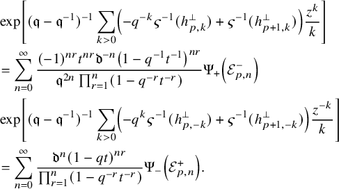 $$ \begin{align*} &\exp\left[(\mathfrak{q}-\mathfrak{q}^{-1})^{-1} \sum_{k>0}\left(-q^{- k}\varsigma^{-1}(h_{p, k}^{\perp})+\varsigma^{-1}(h_{p+1, k}^{\perp}) \right)\frac{z^{ k}}{k} \right]\\ &= \sum_{n=0}^\infty\frac{(-1)^{nr}t^{nr}\mathfrak{d}^{-n}\left( 1-q^{-1}t^{-1} \right)^{nr}}{\mathfrak{q}^{2n}\prod_{r=1}^n\left( 1-q^{-r}t^{-r} \right)}\Psi_+\left( \mathcal{E}_{p,n}^-\right)\\ &\exp\left[(\mathfrak{q}-\mathfrak{q}^{-1})^{-1} \sum_{k>0}\left(-q^{ k}\varsigma^{-1}(h_{p,- k}^{\perp})+\varsigma^{-1}(h_{p+1,- k}^{\perp}) \right)\frac{z^{- k}}{k} \right]\\ &= \sum_{n=0}^\infty\frac{\mathfrak{d}^n\left( 1-qt \right)^{nr}}{\prod_{r=1}^n\left( 1-q^{-r}t^{-r} \right)}\Psi_-\left( \mathcal{E}_{p,n}^+\right). \end{align*} $$
Applying $\eta $
, we get
$\eta $
, we get
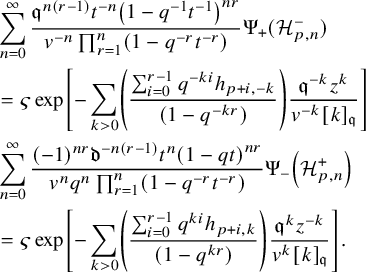 $$ \begin{align*} &\sum_{n=0}^\infty\frac{\mathfrak{q}^{n(r-1)}t^{-n}\left( 1-q^{-1}t^{-1} \right)^{nr}}{v^{-n}\prod_{r=1}^n\left( 1-q^{-r}t^{-r} \right)} \Psi_+(\mathcal{H}^-_{p,n})\\ &= \varsigma\exp\left[-\sum_{k>0}\left(\frac{\sum_{i=0}^{r-1}q^{- ki}h_{p+i,- k}}{(1-q^{- kr})}\right)\frac{\mathfrak{q}^{- k} z^{ k}}{v^{-k}[ k]_{\mathfrak{q}}} \right]\\&\sum_{n=0}^\infty\frac{(-1)^{nr}\mathfrak{d}^{-n(r-1)}t^{n}\left(1- qt \right)^{nr}}{v^nq^{n}\prod_{r=1}^n\left(1- q^{-r}t^{-r} \right)} \Psi_-\left( \mathcal{H}_{p,n}^+ \right)\\ &=\varsigma\exp\left[-\sum_{k>0}\left(\frac{\sum_{i=0}^{r-1}q^{ ki}h_{p+i, k}}{(1-q^{ kr})}\right)\frac{\mathfrak{q}^{ k} z^{- k}}{v^k[ k]_{\mathfrak{q}}} \right]. \end{align*} $$
A.3 Normal ordering
It will be slightly nicer to reorder our currents differently from Proposition 3.7:
Proposition A.2. For $p\in I$
, we have
$p\in I$
, we have
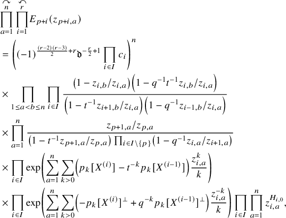 $$ \begin{align*} &\overset{\curvearrowright}{\prod_{a=1}^n}\,\overset{\curvearrowleft}{\prod_{i=1}^{r}}E_{p+i}(z_{p+i,a})\\ &= \left( (-1)^{\frac{(r-2)(r-3)}{2}+r}\mathfrak{d}^{-\frac{r}{2}+1}\prod_{i\in I} c_i\right)^n\\ &\times\prod_{1\le a<b\le n}\prod_{i\in I} \frac{\displaystyle\left(1-z_{i,b}/z_{i,a}\right)\left(1-q^{-1}t^{-1}z_{i,b}/z_{i,a}\right)}{\displaystyle\left(1-t^{-1}z_{i+1,b}/z_{i,a}\right)\left(1-q^{-1}z_{i-1,b}/z_{i,a}\right)}\\ &\times\prod_{a=1}^n \frac{z_{p+1,a}/z_{p,a}} {\left(1-t^{-1}z_{p+1,a}/z_{p,a}\right) \prod_{i\in I\setminus\{p\}} \left(1-q^{-1}z_{i,a}/z_{i+1,a}\right)}\\ &\times\prod_{i\in I}\exp\left(\sum_{a=1}^n\sum_{k>0}\left(p_{k}[X^{(i)}]-t^{-k}p_k[X^{(i-1)}]\right)\frac{z_{i,a}^{k}}{k}\right)\\ &\times\prod_{i\in I}\exp\left(\sum_{a=1}^n\sum_{k>0}\left(-p_{k}[X^{(i)}]^{\perp}+q^{-k}p_k[X^{(i-1)}]^{\perp}\right)\frac{z_{i,a}^{-k}}{k}\right) \prod_{i\in I}\prod_{a=1}^n z_{i,a}^{H_{i,0}}, \end{align*} $$
where all rational functions are Laurent series expanded assuming
 $$ \begin{align} |z_{i,a}|=1,\, |q|>1,\, |t|>1. \end{align} $$
For the F-currents, we have
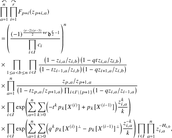 $$ \begin{align*} &\overset{\curvearrowleft}{\prod_{a=1}^n}\,\overset{\curvearrowright}{\prod_{i=1}^{r}}F_{p+i}(z_{p+i,a})\\ &=\left( \frac{(-1)^{\frac{(r-2)(r-3)}{2}+r}\mathfrak{d}^{\frac{r}{2}-1}}{\displaystyle\prod_{i\in I}c_i}\right)^n\\ &\times\prod_{1\le a<b\le n}\prod_{i\in I} \frac{\left(1-z_{i,a}/z_{i,b}\right)\left(1-qtz_{i,a}/z_{i,b}\right)}{\left(1-tz_{i-1,a}/z_{i,b}\right)\left(1-qz_{i+1,a}/z_{i,b}\right)} \\&\times \prod_{a=1}^n\frac{z_{p,a}/z_{p+1,a}}{\left(1-tz_{p,a}/z_{p+1,a}\right) \prod_{i\in I\setminus\{p+1\}} \left(1-qz_{i,a}/z_{i-1,a}\right)}\\&\times\prod_{i\in I}\exp\left(\sum_{a=1}^n\sum_{k>0}\left(-t^{k}p_{k}[X^{(i)}]+p_k[X^{(i-1)}]\right)\frac{z_{i,a}^{k}}{k}\right)\\ &\times\prod_{i\in I}\exp\left(\sum_{a=1}^n\sum_{k>0}\left(q^{k}p_{k}[X^{(i)}]^{\perp}-p_k[X^{(i-1)}]^{\perp}\right)\frac{z_{i,a}^{-k}}{k}\right) \prod_{i\in I}\prod_{a=1}^n z_{i,a}^{-H_{i,0}}, \end{align*} $$
where all rational functions are Laurent series expanded assuming
 $$ \begin{align} |z_{i,a}|=1,\, |q|< 1,\, |t|<1. \end{align} $$
A.4 Integral formula
Let
 $$ \begin{align*} d_n^+&=\frac{\mathfrak{q}^{n(r-1)}t^{-n}\left( 1-q^{-1}t^{-1} \right)^{nr}}{v^{-n}\prod_{r=1}^n\left( 1-q^{-r}t^{-r} \right)},& d_n^-&= \frac{(-1)^{nr}\mathfrak{d}^{-n(r-1)}t^{n}\left(1- qt \right)^{nr}}{v^nq^{n}\prod_{r=1}^n\left(1- q^{-r}t^{-r} \right)}. \end{align*} $$
We have
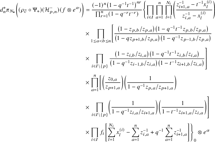 $$ \begin{align*} d_n^+\pi_{N_{\bullet}}\bigg( \left( \rho_{\vec{c}}\circ\Psi_+ \right)(\mathcal{H}_{p,n}^-)(f\otimes e^\alpha)\bigg) &=\frac{(-1)^n\left(1- q^{-1}t^{-1} \right)^{nr}}{\prod_{r=1}^n\left(1- q^{-r}t^{-r} \right)} \left\{\prod_{i\in I}\prod_{a=1}^n\prod_{l=1}^{N_i}\left(\frac{ z_{i+1,a}^{-1}-t^{-1}x_{l}^{(i)} }{ z_{i,a}^{-1}-x_{l}^{(i)} }\right)\right.\\[4pt] &\times\prod_{1\le a<b\le n} \left[ \frac{\left(1-z_{p,b}/z_{p,a}\right)\left(1-q^{-1}t^{-1}z_{p,b}/z_{p,a}\right)}{\left(1-qz_{p+1,b}/z_{p,a}\right)\left(1-q^{-1}z_{p-1,b}/z_{p,a}\right)}\right.\\[4pt] \nonumber &\times\left.\prod_{i\in I\backslash\{p\}} \frac{\left(1-z_{i,b}/z_{i,a}\right)\left(1-q^{-1}t^{-1}z_{i,b}/z_{i,a}\right)}{\left(1-q^{-1}z_{i-1,b}/z_{i,a}\right)\left(1-t^{-1}z_{i+1,b}/z_{i,a}\right)}\right]\\[4pt] &\times\prod_{a=1}^n \left[ \left(\frac{z_{0,a}}{z_{p+1,a}}\right)\left(\frac{1}{1-q^{-1}z_{p,a}/z_{p+1,a}}\right)\right.\\[4pt] \nonumber &\times\left. \prod_{i\in I\setminus\{p\}} \left(\frac{1}{1-q^{-1}z_{i,a}/z_{i+1,a}}\right) \left( \frac{1}{1-t^{-1}z_{i+1,a}/z_{i,a}} \right)\right]\\[4pt] &\times \prod_{i\in I}f_i\left[ \sum_{l=1}^{N_i}x_{l}^{(i)}-\sum_{a=1}^nz_{i,a}^{-1}+q^{-1}\sum_{a=1}^n z_{i+1,a}^{-1} \right]\Bigg\}_0\otimes e^\alpha \end{align*} $$
and
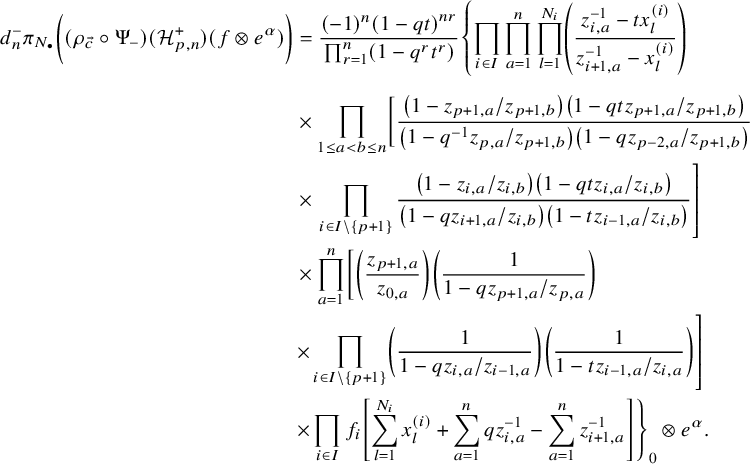 $$ \begin{align*} d_n^-\pi_{N_{\bullet}}\bigg( \left( \rho_{\vec{c}}\circ\Psi_- \right)(\mathcal{H}_{p,n}^+)(f\otimes e^\alpha)\bigg) &= \frac{(-1)^n\left(1- qt \right)^{nr}}{\prod_{r=1}^n\left(1- q^{r}t^{r} \right)} \left\{\prod_{i\in I}\prod_{a=1}^n\prod_{l=1}^{N_i}\left(\frac{ z_{i,a}^{-1}-tx_{l}^{(i)} }{ z_{i+1,a}^{-1}-x_{l}^{(i)} }\right)\right.\\[5pt] &\times\prod_{1\le a<b\le n}\left[ \frac{\left(1-z_{p+1,a}/z_{p+1,b}\right)\left(1-qtz_{p+1,a}/z_{p+1,b}\right)}{\left(1-q^{-1}z_{p,a}/z_{p+1,b}\right)\left(1-qz_{p-2,a}/z_{p+1,b}\right)}\right.\\&\times\left. \prod_{i\in I\backslash\{p+1\}} \frac{\left(1-z_{i,a}/z_{i,b}\right)\left(1-qtz_{i,a}/z_{i,b}\right)}{\left(1-qz_{i+1,a}/z_{i,b}\right)\left(1-tz_{i-1,a}/z_{i,b}\right)}\right]\\ &\times \prod_{a=1}^n \left[ \left(\frac{z_{p+1,a}}{z_{0,a}}\right) \left(\frac{1} {1-qz_{p+1,a}/z_{p,a}}\right)\right.\\ &\left.\times\prod_{i\in I\setminus\{p+1\}} \left(\frac{1}{1-qz_{i,a}/z_{i-1,a}}\right)\left(\frac{1}{1-tz_{i-1,a}/z_{i,a}}\right) \right]\\ &\left.\times \prod_{i\in I} f_i\left[ \sum_{l=1}^{N_i} x_{l}^{(i)}+\sum_{a=1}^n qz_{i,a}^{-1}-\sum_{a=1}^n z_{i+1,a}^{-1} \right]\right\}_0\otimes e^\alpha. \end{align*} $$
Finally, we make the substitution $w_{i,a}=z_{i,a}^{-1}$
and rewrite these formulas in terms of integrals. This gets us
$w_{i,a}=z_{i,a}^{-1}$
and rewrite these formulas in terms of integrals. This gets us
 $$ \begin{align*} &d_n^+\pi_{N_{\bullet}}\bigg( \left( \rho_{\vec{c}}\circ\Psi_+ \right)(\mathcal{H}_{p,n}^-)(f\otimes e^\alpha)\bigg)\\ &=\underset{|w_{i,a}|=1}{\oint\cdots\oint} \bigg(\varrho_{p,n}^+(w_{\bullet,\bullet},X_{N_{\bullet}})\prod_{i\in I} f_i\left[ \sum_{l=1}^{N_i} x_{l}^{(i)}-\sum_{a=1}^nw_{i,a}+\sum_{a=1}^nq^{-1}w_{i+1,a} \right] \prod_{a=1}^n \frac{dw_{i,a}}{2\pi\sqrt{-1}w_{i,a}} \bigg)\otimes e^\alpha \end{align*} $$
and
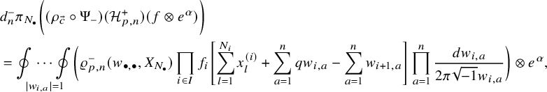 $$ \begin{align*} &d_n^-\pi_{N_{\bullet}}\bigg( \left( \rho_{\vec{c}}\circ\Psi_- \right)(\mathcal{H}_{p,n}^+)(f\otimes e^\alpha)\bigg)\\ &=\underset{|w_{i,a}|=1}{\oint\cdots\oint}\bigg(\varrho_{p,n}^-(w_{\bullet,\bullet},X_{N_{\bullet}})\prod_{i\in I}f_i\left[ \sum_{l=1}^{N_i} x_{l}^{(i)}+\sum_{a=1}^nqw_{i,a}-\sum_{a=1}^nw_{i+1,a} \right] \prod_{a=1}^n \frac{dw_{i,a}}{2\pi\sqrt{-1}w_{i,a}} \bigg)\otimes e^\alpha, \end{align*} $$
where
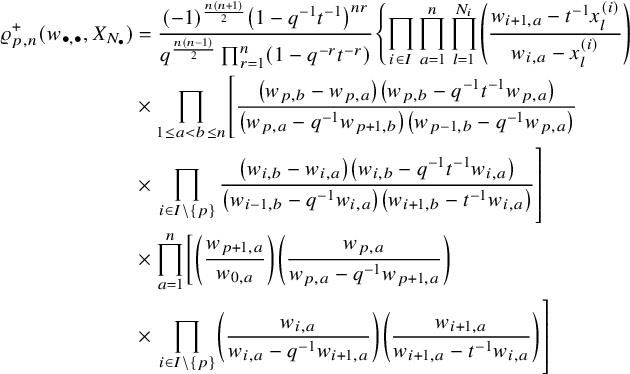 $$ \begin{align*} \varrho_{p,n}^+(w_{\bullet,\bullet},X_{N_{\bullet}}) &= \frac{(-1)^{\frac{n(n+1)}{2}}\left(1- q^{-1}t^{-1} \right)^{nr}}{q^{\frac{n(n-1)}{2}}\prod_{r=1}^n\left(1- q^{-r}t^{-r} \right)} \left\{\prod_{i\in I}\prod_{a=1}^n\prod_{l=1}^{N_i}\left(\frac{ w_{i+1,a}-t^{-1}x_{l}^{(i)} }{ w_{i,a}-x_{l}^{(i)} }\right)\right.\\ &\times\prod_{1\le a<b\le n} \left[ \frac{\left(w_{p,b}-w_{p,a}\right)\left(w_{p,b}-q^{-1}t^{-1}w_{p,a}\right)}{\left(w_{p,a}-q^{-1}w_{p+1,b}\right)\left(w_{p-1,b}-q^{-1}w_{p,a}\right)}\right.\\ \nonumber &\times\left.\prod_{i\in I\backslash\{p\}} \frac{\left(w_{i,b}-w_{i,a}\right)\left(w_{i,b}-q^{-1}t^{-1}w_{i,a}\right)}{\left(w_{i-1,b}-q^{-1}w_{i,a}\right)\left(w_{i+1,b}-t^{-1}w_{i,a}\right)}\right]\\ &\times\prod_{a=1}^n \left[ \left(\frac{w_{p+1,a}}{w_{0,a}}\right)\left(\frac{w_{p,a}}{w_{p,a}-q^{-1}w_{p+1,a}}\right)\right.\\ \nonumber &\times\left. \prod_{i\in I\setminus\{p\}} \left(\frac{w_{i,a}}{w_{i,a}-q^{-1}w_{i+1,a}}\right) \left( \frac{w_{i+1,a}}{w_{i+1,a}-t^{-1}w_{i,a}} \right)\right] \end{align*} $$
and
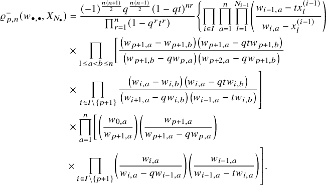 $$ \begin{align*} \varrho_{p,n}^-(w_{\bullet,\bullet},X_{N_{\bullet}}) &= \frac{(-1)^{\frac{n(n+1)}{2}}q^{\frac{n(n-1)}{2}}\left(1- qt \right)^{nr}}{\prod_{r=1}^n\left(1- q^{r}t^{r} \right)} \left\{\prod_{i\in I}\prod_{a=1}^n\prod_{l=1}^{N_{i-1}}\left(\frac{ w_{i-1,a}-tx_{l}^{(i-1)} }{ w_{i,a}-x_{l}^{(i-1)} }\right)\right.\\ &\times\prod_{1\le a<b\le n}\left[ \frac{\left(w_{p+1,a}-w_{p+1,b}\right)\left(w_{p+1,a}-qtw_{p+1,b}\right)}{\left(w_{p+1,b}-qw_{p,a}\right)\left(w_{p+2,a}-qw_{p+1,b}\right)}\right.\\ &\times\left. \prod_{i\in I\backslash\{p+1\}} \frac{\left(w_{i,a}-w_{i,b}\right)\left(w_{i,a}-qtw_{i,b}\right)}{\left(w_{i+1,a}-qw_{i,b}\right)\left(w_{i-1,a}-tw_{i,b}\right)}\right]\\ &\times \prod_{a=1}^n \left[ \left(\frac{w_{0,a}}{w_{p+1,a}}\right) \left(\frac{w_{p+1,a}}{w_{p+1,a}-qw_{p,a}}\right)\right.\\ &\left.\times\prod_{i\in I\setminus\{p+1\}} \left(\frac{w_{i,a}}{w_{i,a}-qw_{i-1,a}}\right)\left(\frac{w_{i-1,a}}{w_{i-1,a}-tw_{i,a}}\right) \right]. \end{align*} $$
A.5 Degree one
We compute the integral and record the resulting action on f when $n=1$
.
$n=1$
.
A.5.1 Difference operators
Let $Sh(X_{N_{\bullet }})=Sh$
denote the set of all shift patterns. Define
$Sh(X_{N_{\bullet }})=Sh$
denote the set of all shift patterns. Define
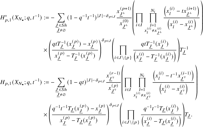 $$ \begin{align*} H_{p,1}^*(X_{N_{\bullet}};q,t^{-1}) &:= -\sum_{\substack{{\underline{J}}\in Sh\\{\underline{J}}\not=\varnothing}}(1-q^{-1}t^{-1})^{|J|-\delta_{p\in J}} \frac{x^{(p+1)}_{{\underline{J}}^{\vartriangle}}}{x^{(0)}_{{\underline{J}}^{\vartriangle}}} \left( \prod_{i\in I}\prod_{\substack{l=1\\ x^{(i)}_{l}\not=x^{(i)}_{{\underline{J}}^\vartriangle}}}^{N_i}\frac{\left(x_{l}^{(i)}-tx^{(i+1)}_{{\underline{J}}^\vartriangle}\right)}{\left(x_{l}^{(i)}-x^{(i)}_{{\underline{J}}^\vartriangle}\right)} \right)\\ &\times \left( \frac{qtT_{{\underline{J}}}^{-1}(x^{(p)}_{{\underline{J}}})-x^{(p)}_{{\underline{J}}}}{x^{(p)}_{{\underline{J}}}-T_{{\underline{J}}}^{-1}(x^{(p)}_{{\underline{J}}})} \right)^{\delta_{p\in J}} \left(\prod_{i\in J\backslash\{p\}}\frac{qtT_{{\underline{J}}}^{-1}(x^{(i)}_{{\underline{J}}})}{\left(x^{(i)}_{{\underline{J}}}-T_{\underline{J}}^{-1} (x^{(i)}_{{\underline{J}}})\right)}\right) T_{{\underline{J}}}^{-1}\\ H_{p,1}(X_{N_{\bullet}};q,t^{-1}) &:= -\sum_{\substack{{\underline{J}}\in Sh\\{\underline{J}}\not=\varnothing}} (1-qt)^{|J|-\delta_{p\in J}} \frac{x^{(r-1)}_{{\underline{J}}^{\triangledown}}}{x^{(p)}_{{\underline{J}}^{\triangledown}}} \left(\prod_{i\in I}\prod_{\substack{l=1\\ x^{(i)}_{l}\not= x^{(i)}_{{\underline{J}}^{\triangledown}}}}^{N_i} \frac{\left(x^{(i)}_{l}-t^{-1}x^{(i-1)}_{{\underline{J}}^{\triangledown}}\right)}{\left(x^{(i)}_{l}-x^{(i)}_{{\underline{J}}^{\triangledown}}\right)}\right)\\ &\times\left( \frac{q^{-1}t^{-1}T_{{\underline{J}}}(x^{(p)}_{{\underline{J}}})-x^{(p)}_{{\underline{J}}}}{x^{(p)}_{{\underline{J}}}-T_{{\underline{J}}}(x^{(p)}_{{\underline{J}}})} \right)^{\delta_{p\in J}} \left(\prod_{i\in J\backslash\{p\}}\frac{q^{-1}t^{-1}T_{{\underline{J}}}(x^{(i)}_{{\underline{J}}})}{\left(x^{(i)}_{{\underline{J}}}-T_{\underline{J}} (x^{(i)}_{{\underline{J}}})\right)}\right) T_{{\underline{J}}}. \end{align*} $$
Setting $r=1$
and inverting t, we indeed obtain the first Noumi-Sano operator.
$r=1$
and inverting t, we indeed obtain the first Noumi-Sano operator.
A.5.2 Eigenvalues
For a series $f(z)$
in z, let
$f(z)$
in z, let $[z^n] f(z)$
denote the coefficient of
$[z^n] f(z)$
denote the coefficient of $z^n$
. Methods similar to those in 5.4 allow us to establish the following.
$z^n$
. Methods similar to those in 5.4 allow us to establish the following.
Theorem A.3. For $|q|>1$
, we have
$|q|>1$
, we have
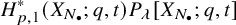 $$ \begin{align} &\hspace{-70pt}H^*_{p,1}(X_{N_{\bullet}};q,t)P_{\lambda}[X_{N_{\bullet}};q,t] \end{align} $$
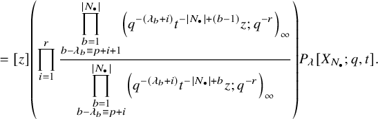 $$ \begin{align} &= [z]\left( \prod_{i=1}^{r} \frac{\displaystyle\prod^{|N_{\bullet}|}_{\substack{b=1\\ b-\lambda_b\equiv p+i+1 }}\left(q^{-(\lambda_b+i)}t^{-|N_{\bullet}|+ (b- 1)}z; q^{- r}\right)_\infty} {\displaystyle\prod^{|N_{\bullet}|}_{\substack{b=1\\ b-\lambda_b\equiv p+i }}\left(q^{-(\lambda_b+i)}t^{-|N_{\bullet}| +b}z; q^{- r}\right)_\infty} \right)P_{\lambda}[X_{N_{\bullet}};q,t]. \end{align} $$
However, for $|q|<1$
, we have
$|q|<1$
, we have
 $$ \begin{align} &\hspace{-70pt}H_{p,1}(X_{N_{\bullet}};q,t)P_{\lambda}[X_{N_{\bullet}};q,t] \end{align} $$
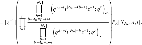 $$ \begin{align} &= [z^{-1}]\left( \prod_{i=1}^{r} \frac{\displaystyle\prod^{|N_{\bullet}|}_{\substack{b=1\\ b-\lambda_b\equiv p+i+1 }}\left(q^{\lambda_b+i}t^{|N_{\bullet}|- (b- 1)}z^{-1}; q^{ r}\right)_\infty} {\displaystyle\prod^{|N_{\bullet}|}_{\substack{b=1\\ b-\lambda_b\equiv p+i }}\left(q^{\lambda_b+i}t^{|N_{\bullet}| -b}z^{-1}; q^{ r}\right)_\infty} \right)P_{\lambda}[X_{N_{\bullet}};q,t]. \end{align} $$
Remark A.4. We have presented the eigenvalues in terms of our original spectral variables $q^{\lambda _b}t^{|N_{\bullet }|-b}$
. However, we can give a more natural combinatorial expression for the eigenvalues if we forgo this and use instead the transpose partition
$q^{\lambda _b}t^{|N_{\bullet }|-b}$
. However, we can give a more natural combinatorial expression for the eigenvalues if we forgo this and use instead the transpose partition $\lambda '$
[Reference Macdonald9, (I.1.3)]. Let
$\lambda '$
[Reference Macdonald9, (I.1.3)]. Let
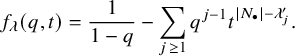 $$ \begin{align} f_{\lambda}(q,t) = \dfrac{1}{1-q} - \sum_{j\ge 1} q^{j-1} t^{|N_{\bullet}|-\lambda'_j}. \end{align} $$
It can be viewed as a series or as a rational function since $(1-q^r) f_{\lambda }(q,t)$
is a polynomial. Let
$(1-q^r) f_{\lambda }(q,t)$
is a polynomial. Let $\Gamma =\mathbb {Z}/r\mathbb {Z}$
be the cyclic group and let
$\Gamma =\mathbb {Z}/r\mathbb {Z}$
be the cyclic group and let $\chi $
be the generator of
$\chi $
be the generator of $R(\Gamma )$
. Define
$R(\Gamma )$
. Define $f_{\lambda }^{(p)}(q,t)$
by the following expression in
$f_{\lambda }^{(p)}(q,t)$
by the following expression in $\mathbb {Q}(q,t) \otimes R(\Gamma )$
:
$\mathbb {Q}(q,t) \otimes R(\Gamma )$
:
 $$ \begin{align} f_{\lambda}(q\chi^{-1},t\chi^{-1}) = \chi^{-1}\sum_{p\in I} f^{(p)}_{\lambda}(q,t) \chi^p. \end{align} $$
Then the eigenvalues are given by
 $$ \begin{align} H^*_{p,1}(X_{N_{\bullet}};q,t) P_{\lambda}[X_{N_{\bullet}};q,t] &= f_{\lambda}^{(p)}(q^{-1},t^{-1}) P_{\lambda}[X_{N_{\bullet}};q,t] \end{align} $$
 $$ \begin{align} H_{p,1}(X_{N_{\bullet}};q,t) P_{\lambda}[X_{N_{\bullet}};q,t] &= f_{\lambda}^{(p)}(q,t) P_{\lambda}[X_{N_{\bullet}};q,t]. \end{align} $$
Example A.5. Let $r=2$
and
$r=2$
and $\alpha =0$
(empty core). We use
$\alpha =0$
(empty core). We use $N_0=N_1=1$
. There are three nonempty shift patterns:
$N_0=N_1=1$
. There are three nonempty shift patterns: ${\underline {J}}_1 = \{x_1^{(0)}\}$
,
${\underline {J}}_1 = \{x_1^{(0)}\}$
, ${\underline {J}}_2=\{x_1^{(1)}\}$
and
${\underline {J}}_2=\{x_1^{(1)}\}$
and ${\underline {J}}_3 = \{x_1^{(0)},x_1^{(1)}\}$
. We apply
${\underline {J}}_3 = \{x_1^{(0)},x_1^{(1)}\}$
. We apply $H_{0,1}[X_{{N_{\bullet }}};q,t^{-1}]$
to
$H_{0,1}[X_{{N_{\bullet }}};q,t^{-1}]$
to $P_\emptyset [X_{{N_{\bullet }}};q,t]=1$
using summands
$P_\emptyset [X_{{N_{\bullet }}};q,t]=1$
using summands ${\underline {J}}_1,{\underline {J}}_2,{\underline {J}}_3$
:
${\underline {J}}_1,{\underline {J}}_2,{\underline {J}}_3$
:
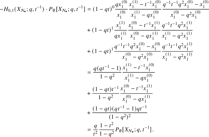 $$ \begin{align*} - H_{0,1}(X_{{N_{\bullet}}};q,t^{-1})\cdot P_\emptyset[X_{{N_{\bullet}}};q,t^{-1}] &= (1-qt)^0 \dfrac{q x_1^{(0)}}{x_1^{(0)}} \dfrac{x_1^{(1)}-t^{-1} x_1^{(0)}}{x_1^{(1)}-q x_1^{(0)}} \dfrac{q^{-1}t^{-1} q^2 x_1^{(0)} - x_1^{(0)}}{x_1^{(0)}-q^2 x_1^{(0)}} \\ &+ (1-qt)^1 \dfrac{x_1^{(1)}}{q x_1^{(1)}} \dfrac{x_1^{(0)}-t^{-1} x_1^{(1)}}{x_1^{(0)}-q x_1^{(1)}} \dfrac{q^{-1}t^{-1}q^2 x_1^{(1)}}{x_1^{(1)}-q^2x_1^{(1)}} \\ &+ (1-qt)^1 \dfrac{q^{-1}t^{-1} q^2 x_1^{(0)}- x_1^{(0)}}{x_1^{(0)}-q^2 x_1^{(0)}} \dfrac{q^{-1}t^{-1} q^2 x_1^{(1)}}{x_1^{(1)}-q^2 x_1^{(1)}}\\ &= \dfrac{q (qt^{-1}-1)}{1-q^2} \dfrac{x_1^{(1)}-t^{-1} x_1^{(0)}}{x_1^{(1)}-qx_1^{(0)}} \\ &+\dfrac{(1-qt)t^{-1}}{1-q^2}\dfrac{x_1^{(0)}-t^{-1}x_1^{(1)}}{x_1^{(0)}-qx_1^{(1)}}\\ &+\dfrac{(1-qt)(qt^{-1}-1)qt^{-1}}{(1-q^2)^2} \\ &= \dfrac{q}{t^2} \dfrac{1-t^2}{1-q^2} P_{\emptyset}[X_{{N_{\bullet}}};q,t^{-1}]. \end{align*} $$
We have
 $$ \begin{align*} f_{\emptyset}(q,t) &= \dfrac{1}{1-q} - \dfrac{t^2}{1-q} = \dfrac{1-t^2}{1-q} \\ f_{\emptyset}(q\chi^{-1},t\chi^{-1}) &= \dfrac{1-t^2}{1-q^2} (1 + q \chi) \\ f_{\emptyset}^{(0)}(q,t) &= q \dfrac{1-t^2}{1-q^2} \\ f_{\emptyset}^{(0)}(q,t^{-1}) &= q \dfrac{1-t^{-2}}{1-q^2} = - \dfrac{q}{t^2} \dfrac{1-t^2}{1-q^2}. \end{align*} $$
Acknowledgements
We thank Mark Haiman, Andrei Neguţ and Alexander Tsymbaliuk for helpful conversations.
Competing interest
The authors have no competing interests to declare.
Funding statement
D.O. gratefully acknowledges support from the Simons Foundation (638577, MPS-TSM-00008136) and the Max Planck Institute for Mathematics (MPIM Bonn). J.J.W. was supported by NSF-RTG grant ‘Algebraic Geometry and Representation Theory at Northeastern University’ (DMS-1645877) and ERC consolidator grant No. 101001159 ‘Refined invariants in combinatorics, low-dimensional topology and geometry of moduli spaces’.
Data availability statement
Not applicable
Ethical standards
The research meets all ethical guidelines, including adherence to the legal requirements of the study country.
Author contributions
All three authors contributed equally to this work.


 Open access