


1. Introduction
This paper, which is the last in a series of three [Reference Borodzik, Conway and Politarczyk1, Reference Borodzik, Conway and Politarczyk2], illustrates how to compute algorithmically certain signature invariants of a knot $K$
, twisted by a representation
$K$
, twisted by a representation $\pi _1(X_K) \to GL_d({\mathbb{F}[t^{\pm 1}]})$
, where
$\pi _1(X_K) \to GL_d({\mathbb{F}[t^{\pm 1}]})$
, where $X_K$
denotes the exterior of
$X_K$
denotes the exterior of $K$
. Before describing this algorithm, we provide some background on twisted Blanchfield forms and twisted signature invariants.
$K$
. Before describing this algorithm, we provide some background on twisted Blanchfield forms and twisted signature invariants.
1.1. Classical knot theory
Classical knot theory is concerned with knot invariants that are extracted from the algebraic topology of the knot exterior. Here, given a knot $K$
, customary notation involves using
$K$
, customary notation involves using $\nu (K)$
for an open tubular neighbourhood of
$\nu (K)$
for an open tubular neighbourhood of $K$
and
$K$
and $X_K\;:\!=\;S^3 \setminus \nu (K)$
for the exterior of
$X_K\;:\!=\;S^3 \setminus \nu (K)$
for the exterior of $K$
. Textbook examples of classical knot invariants include the Alexander polynomial
$K$
. Textbook examples of classical knot invariants include the Alexander polynomial $\Delta _K$
and the Levine-Tristram signature
$\Delta _K$
and the Levine-Tristram signature $\sigma _K \colon S^1 \to \mathbb{Z}$
[Reference Lickorish27, Reference Rolfsen38].
$\sigma _K \colon S^1 \to \mathbb{Z}$
[Reference Lickorish27, Reference Rolfsen38].
Both of these invariants are extracted from the infinite cyclic cover $X_K^\infty \to X_K$
and can be calculated using Seifert surfaces, that is, compact, connected, oriented surfaces in
$X_K^\infty \to X_K$
and can be calculated using Seifert surfaces, that is, compact, connected, oriented surfaces in $S^3$
with boundary
$S^3$
with boundary $K$
. Indeed, given a Seifert matrix
$K$
. Indeed, given a Seifert matrix $A$
for
$A$
for $K$
, the Alexander polynomial and signature at
$K$
, the Alexander polynomial and signature at $\omega \in S^1$
can be expressed as
$\omega \in S^1$
can be expressed as
 \begin{align*} &\Delta _K(t)=\det\!(tA-A^T),\\[5pt] &\sigma _K(\omega )=\operatorname{sign}\!((1-\omega )A+(1- \overline{\omega })A^T). \end{align*}
The same goes for the Alexander module $H_1(X_K;\;\mathbb{Z}[t^{\pm 1 }])\;:\!=\;H_1(X_K^\infty )$
which is presented, as a
$H_1(X_K;\;\mathbb{Z}[t^{\pm 1 }])\;:\!=\;H_1(X_K^\infty )$
which is presented, as a $\mathbb{Z}[t^{\pm 1}]$
-module, by the matrix
$\mathbb{Z}[t^{\pm 1}]$
-module, by the matrix $tA-A^T$
.
$tA-A^T$
.
Another classical knot invariant, that appears less frequently in textbooks, is a non-singular, sesquilinear, Hermitian form
 \begin{equation*} \textrm {Bl}(K) \colon H_1(X_K;\;\mathbb {Z}[t^{\pm 1}]) \times H_1(X_K;\;\mathbb {Z}[t^{\pm 1}]) \to \mathbb {Q}(t)/\mathbb {Z}[t^{\pm 1}],\end{equation*}
known as the Blanchfield form. Sesquilinearity refers to the fact that $\textrm{Bl}(K)(px,qy)=p\overline{q}\textrm{Bl}(K)(x,y)$
for every
$\textrm{Bl}(K)(px,qy)=p\overline{q}\textrm{Bl}(K)(x,y)$
for every $x,y \in H_1(X_K;\;\mathbb{Z}[t^{\pm 1}])$
(where, given a rational function
$x,y \in H_1(X_K;\;\mathbb{Z}[t^{\pm 1}])$
(where, given a rational function $p\;:\!=\;p(t) \in \mathbb{Q}(t)$
, we write
$p\;:\!=\;p(t) \in \mathbb{Q}(t)$
, we write $\overline{p}\;:\!=\;p(t^{-1})$
) and
$\overline{p}\;:\!=\;p(t^{-1})$
) and $\textrm{Bl}(K)$
being Hermitian means that
$\textrm{Bl}(K)$
being Hermitian means that $\textrm{Bl}(K)(y,x)=\overline{\textrm{Bl}(K)(x,y)}$
. The Blanchfield form can also be expressed using Seifert matrices [Reference Friedl and Powell13, Reference Kearton21]. The data of the pair
$\textrm{Bl}(K)(y,x)=\overline{\textrm{Bl}(K)(x,y)}$
. The Blanchfield form can also be expressed using Seifert matrices [Reference Friedl and Powell13, Reference Kearton21]. The data of the pair $(H_1(X_K;\;\mathbb{Z}[t^{\pm 1}]),\textrm{Bl}(K))$
encapsulate both the Alexander polynomial and the signature:
$(H_1(X_K;\;\mathbb{Z}[t^{\pm 1}]),\textrm{Bl}(K))$
encapsulate both the Alexander polynomial and the signature: $H_1(X_K;\;\mathbb{Z}[t^{\pm 1}])$
determines
$H_1(X_K;\;\mathbb{Z}[t^{\pm 1}])$
determines $\Delta _K$
and
$\Delta _K$
and $\textrm{Bl}(K)$
determines
$\textrm{Bl}(K)$
determines $\sigma _K$
.
$\sigma _K$
.
Applications of classical invariants include the study of the unknotting number, the $3$
-genus, fibredness as well as questions related to
$3$
-genus, fibredness as well as questions related to $4$
-dimensional topology and knot concordance. Here knot concordance refers to the study of (topologically) slice knots, that is, knots that bound a locally flat disc in
$4$
-dimensional topology and knot concordance. Here knot concordance refers to the study of (topologically) slice knots, that is, knots that bound a locally flat disc in $D^4$
.
$D^4$
.
1.2. Twisted knot invariants
More recently, knot theorists have taken up the study of invariants of pairs $(K,\beta )$
, where
$(K,\beta )$
, where $K$
is a knot and
$K$
is a knot and $\beta \colon \pi _1(X_K) \to GL_d({\mathbb{F}[t^{\pm 1}]})$
is a representation; (in fact, instead of the exterior
$\beta \colon \pi _1(X_K) \to GL_d({\mathbb{F}[t^{\pm 1}]})$
is a representation; (in fact, instead of the exterior $X_K$
, it is often convenient to use the closed
$X_K$
, it is often convenient to use the closed $3$
-manifold
$3$
-manifold $M_K$
obtained from
$M_K$
obtained from $S^3$
by
$S^3$
by $0$
-framed surgery on
$0$
-framed surgery on $K$
). The idea is that classical invariants correspond to the case where
$K$
). The idea is that classical invariants correspond to the case where $\beta$
is induced by abelianisation, whereas non-abelian representations capture more information about the fundamental group.
$\beta$
is induced by abelianisation, whereas non-abelian representations capture more information about the fundamental group.
The first papers on the topic, such as [Reference Kirk and Livingston23, Reference Lin28], focused on twisted Alexander polynomials, but the theory has also been leveraged to construct signature invariants [Reference Cha8, Reference Friedl14, Reference Kirk and Livingston23, Reference Levine26, Reference Nosaka34] and arguably has its root in earlier work of Casson and Gordon [Reference Casson and Gordon6, Reference Casson and Gordon7]. Many of the applications and successes of twisted knot invariants are discussed in [Reference Friedl and Vidussi16] but we simply note that one common area of application again concerns the study of knot concordance; see for example, [Reference Friedl14, Reference Friedl15, Reference Herald, Kirk and Livingston19, Reference Kirk and Livingston22, Reference Kirk and Livingston24, Reference Livingston and Meier30, Reference Miller31, Reference Miller32].
More recently, taking inspiration from the work of Cochran-Orr-Teichner [Reference Cochran, Orr and Teichner11], Miller and Powell initiated the study of the twisted Blanchfield form $\textrm{Bl}_\beta (K)$
, also with an eye towards applications to knot concordance group [Reference Miller and Powell33]. The absence of computational tools (such as the Seifert matrix in the classical case) has however limited further applications.
$\textrm{Bl}_\beta (K)$
, also with an eye towards applications to knot concordance group [Reference Miller and Powell33]. The absence of computational tools (such as the Seifert matrix in the classical case) has however limited further applications.
The goal of our sequence of papers is to further develop the theory of twisted Blanchfield forms and signatures, address computational aspects, and obtain further results in knot concordance. Our theory was applied in [Reference Conway, Kim and Politarczyk9] to study the subgroup of the knot concordance group generated by iterated torus knots; see also [Reference Conway and Nagel10].
1.3. Twisted Blanchfield forms and twisted signatures
Given a knot $K \subset S^3$
and a unitary acyclic representation
$K \subset S^3$
and a unitary acyclic representation $\beta \colon \pi _1(M_K) \to GL_d(\mathbb{C}[t^{\pm 1}])$
(we call
$\beta \colon \pi _1(M_K) \to GL_d(\mathbb{C}[t^{\pm 1}])$
(we call $\beta$
acyclic if the
$\beta$
acyclic if the $\mathbb{C}[t^{\pm 1}]$
-module
$\mathbb{C}[t^{\pm 1}]$
-module $H_1(M_K;\;\mathbb{C}[t^{\pm 1}]^d_{\beta })$
is torsion for each
$H_1(M_K;\;\mathbb{C}[t^{\pm 1}]^d_{\beta })$
is torsion for each $i$
), the twisted Blanchfield form is a non-singular, sesquilinear Hermitian pairing
$i$
), the twisted Blanchfield form is a non-singular, sesquilinear Hermitian pairing
 \begin{equation*} \textrm {Bl}_{\beta }(K) \colon H_1(M_K;\;{\mathbb {F}[t^{\pm 1}]}^d_{\beta }) \times H_1(M_K;\;{\mathbb {F}[t^{\pm 1}]}^d_{\beta }) \to \mathbb {C}(t)/\mathbb {C}[t^{\pm 1}].\end{equation*}
Details will be recalled in Section 3, but we nevertheless note two facts. First, when $\beta$
is induced by abelianisation,
$\beta$
is induced by abelianisation, $\textrm{Bl}_{\beta }(K)$
reduces to the classical Blanchfield form
$\textrm{Bl}_{\beta }(K)$
reduces to the classical Blanchfield form $\textrm{Bl}(K)$
. Secondly, while
$\textrm{Bl}(K)$
. Secondly, while $\textrm{Bl}_{\beta }(K)$
has been studied by Powell [Reference Powell35, Reference Powell36] and Miller-Powell [Reference Miller and Powell33], extracting concrete computable invariants from
$\textrm{Bl}_{\beta }(K)$
has been studied by Powell [Reference Powell35, Reference Powell36] and Miller-Powell [Reference Miller and Powell33], extracting concrete computable invariants from $\textrm{Bl}_{\beta }(K)$
has remained challenging. For instance, while
$\textrm{Bl}_{\beta }(K)$
has remained challenging. For instance, while $\textrm{Bl}_{\beta }(K)\,$
has been used to obstruct certain satellite knots from being slice [Reference Miller and Powell33], no explicit calculations have been possible for low crossing knots.
$\textrm{Bl}_{\beta }(K)\,$
has been used to obstruct certain satellite knots from being slice [Reference Miller and Powell33], no explicit calculations have been possible for low crossing knots.
In the first two papers of this series [Reference Borodzik, Conway and Politarczyk1, Reference Borodzik, Conway and Politarczyk2], we proved a classification result for linking forms over $\mathbb{F}[t^{\pm 1}]$
, where
$\mathbb{F}[t^{\pm 1}]$
, where $\mathbb{F}=\mathbb{R},\mathbb{C}$
, and described how to use this result to extract computable signature invariants from
$\mathbb{F}=\mathbb{R},\mathbb{C}$
, and described how to use this result to extract computable signature invariants from $\textrm{Bl}_{\beta }(K)$
, including a new twisted signature function
$\textrm{Bl}_{\beta }(K)$
, including a new twisted signature function
 \begin{equation*} \sigma _{K,\beta } \colon S^1 \to \mathbb {Z}\end{equation*}
that reduces to $\sigma _K$
for abelian
$\sigma _K$
for abelian $\beta$
and that is related to the Casson-Gordon invariants [Reference Casson and Gordon6, Reference Casson and Gordon7] for metabelian
$\beta$
and that is related to the Casson-Gordon invariants [Reference Casson and Gordon6, Reference Casson and Gordon7] for metabelian $\beta$
. We note that the Blanchfield form
$\beta$
. We note that the Blanchfield form $\textrm{Bl}_{\beta }(K)$
(and therefore the signature function
$\textrm{Bl}_{\beta }(K)$
(and therefore the signature function $\sigma _{K,\beta }$
) only depends on the conjugacy class of
$\sigma _{K,\beta }$
) only depends on the conjugacy class of $\beta$
.
$\beta$
.
Thanks to results from [Reference Borodzik, Conway and Politarczyk2] and to formulas for the behaviour of $\textrm{Bl}_{\beta }(K)$
under satellite operations from [Reference Borodzik, Conway and Politarczyk1], this paper shows how twisted signature invariants of iterated torus knots can be understood explicitly.
$\textrm{Bl}_{\beta }(K)$
under satellite operations from [Reference Borodzik, Conway and Politarczyk1], this paper shows how twisted signature invariants of iterated torus knots can be understood explicitly.
Remark 1.1.
The relationship between $\sigma _{K,\beta }$
and Casson-Gordon invariants arises by considering a representation
$\sigma _{K,\beta }$
and Casson-Gordon invariants arises by considering a representation $\alpha _K(n,\chi ) \colon \pi _1(M_K) \to GL_n(\mathbb{C}[t^{\pm 1}])$
, where
$\alpha _K(n,\chi ) \colon \pi _1(M_K) \to GL_n(\mathbb{C}[t^{\pm 1}])$
, where $\chi \colon H_1(\Sigma _n(K);\;\mathbb{Z}) \to \mathbb{Z}_m$
is a character; here,
$\chi \colon H_1(\Sigma _n(K);\;\mathbb{Z}) \to \mathbb{Z}_m$
is a character; here, $\Sigma _n(K)$
denotes the
$\Sigma _n(K)$
denotes the $n$
-fold branched cover of
$n$
-fold branched cover of $K$
. The definition of this representation will be recalled in Section
4
, but, from now on, we refer to
$K$
. The definition of this representation will be recalled in Section
4
, but, from now on, we refer to $\textrm{Bl}_{\alpha (n,\chi )}(K)$
as a metabelian Blanchfield form and to the corresponding signatures as metabelian signatures.
$\textrm{Bl}_{\alpha (n,\chi )}(K)$
as a metabelian Blanchfield form and to the corresponding signatures as metabelian signatures.
1.4. Twisted signatures of iterated torus knots
In order to describe our computation of twisted signatures for (iterated) torus knots, we briefly recall from [Reference Borodzik, Conway and Politarczyk1] how $\sigma _{K,\beta }$
is constructed; more details will be given in Section 3. As we review in Section 2, given a torsion
$\sigma _{K,\beta }$
is constructed; more details will be given in Section 3. As we review in Section 2, given a torsion $\mathbb{C}[t^{\pm 1}]$
-module
$\mathbb{C}[t^{\pm 1}]$
-module $M$
, our work from [Reference Borodzik, Conway and Politarczyk2] associates with every linking form
$M$
, our work from [Reference Borodzik, Conway and Politarczyk2] associates with every linking form $\lambda \colon M \times M \to \mathbb{C}(t)/\mathbb{C}[t^{\pm 1}]$
a locally constant signature function
$\lambda \colon M \times M \to \mathbb{C}(t)/\mathbb{C}[t^{\pm 1}]$
a locally constant signature function
 \begin{equation*} \sigma _{(M,\lambda )} \colon S^1 \to \mathbb {Z}. \end{equation*}
The twisted signature $\sigma _{K,\beta }$
is obtained as the signature function of the linking form
$\sigma _{K,\beta }$
is obtained as the signature function of the linking form $\textrm{Bl}_{\beta }(K)$
. In practice however, instead of describing the signature function, it is often more convenient to describe its value at the points
$\textrm{Bl}_{\beta }(K)$
. In practice however, instead of describing the signature function, it is often more convenient to describe its value at the points $\xi \in S^1$
where it jumps. Without going into details, given
$\xi \in S^1$
where it jumps. Without going into details, given $\xi \in S^1$
, these values are captured by the signature jump
$\xi \in S^1$
, these values are captured by the signature jump
 \begin{equation*} \delta \sigma _{(M,\lambda )}(\xi ) \in \mathbb {Z},\end{equation*}
the collection of which determines $\sigma _{M,\lambda }$
up to an additive constant. In turn, the signature jumps can be explicitly calculated if one knows the isometry type of the linking form
$\sigma _{M,\lambda }$
up to an additive constant. In turn, the signature jumps can be explicitly calculated if one knows the isometry type of the linking form $(M,\lambda )$
. Indeed, every linking form decomposes uniquely as
$(M,\lambda )$
. Indeed, every linking form decomposes uniquely as
 \begin{equation} (M,\lambda )= \bigoplus _{\substack{n_i,\epsilon _i,\xi _i\\ i\in I}}\mathfrak{e}(n_i,\epsilon _i,\xi _i,\mathbb{C})\oplus \bigoplus _{\substack{\xi _j\\ j\in J}}\mathfrak{f}(n_j,\xi _j,\mathbb{C}) \end{equation}
where the summands are explicit linking forms (whose definitions are recalled in Subsection 2) and the value of $\delta \sigma _{(M,\lambda )}(\xi )$
can be read off this decomposition.
$\delta \sigma _{(M,\lambda )}(\xi )$
can be read off this decomposition.
Remark 1.2.
In the decomposition of (1.1), the parameters $n_i \in \mathbb{N}_{\gt 0}$
and
$n_i \in \mathbb{N}_{\gt 0}$
and $\xi _i \in \mathbb{C}$
can be read off the primary decomposition of the module
$\xi _i \in \mathbb{C}$
can be read off the primary decomposition of the module $H$
; the knowledge of the linking form is not necessary. The signs
$H$
; the knowledge of the linking form is not necessary. The signs $\epsilon _i \in \lbrace \pm 1 \rbrace$
can be obtained if one knows the value of the linking form on every pair of elements of the module
$\epsilon _i \in \lbrace \pm 1 \rbrace$
can be obtained if one knows the value of the linking form on every pair of elements of the module ${\mathbb{F}[t^{\pm 1}]}/\textsf{F}_{\xi _i}^{n_i}$
that supports
${\mathbb{F}[t^{\pm 1}]}/\textsf{F}_{\xi _i}^{n_i}$
that supports $\mathfrak{e}(n_i,\epsilon _i,\xi _i,\mathbb{C})$
.
$\mathfrak{e}(n_i,\epsilon _i,\xi _i,\mathbb{C})$
.
Summarising, given a linking form $(M,\lambda )$
, Remark 2.6 below describes an algorithm to obtain the aforementioned decomposition of
$(M,\lambda )$
, Remark 2.6 below describes an algorithm to obtain the aforementioned decomposition of $(M,\lambda )$
and to read off its signature jumps. Thanks to this algorithm, the following theorem leads to a calculation of certain metabelian signatures of the
$(M,\lambda )$
and to read off its signature jumps. Thanks to this algorithm, the following theorem leads to a calculation of certain metabelian signatures of the $(2,2k+1)$
-torus knots.
$(2,2k+1)$
-torus knots.
Theorem 1.3.
For any $k\gt 0$
, there are
$k\gt 0$
, there are $2k+1$
characters
$2k+1$
characters $H_1(\Sigma _2(T_{2,2k+1})) \to \mathbb{Z}_{2k+1}$
which are denoted by
$H_1(\Sigma _2(T_{2,2k+1})) \to \mathbb{Z}_{2k+1}$
which are denoted by $\chi _\theta$
for
$\chi _\theta$
for $\theta =0,\ldots,2k$
. Each of the unitary representations
$\theta =0,\ldots,2k$
. Each of the unitary representations $\alpha (2,\chi _{\theta })$
is acyclic and, for
$\alpha (2,\chi _{\theta })$
is acyclic and, for $\theta =1,\ldots,k$
, the representation
$\theta =1,\ldots,k$
, the representation $\alpha (2,\chi _{\theta })$
is conjugate to
$\alpha (2,\chi _{\theta })$
is conjugate to $\alpha (2,\chi _{2k-\theta })$
.
$\alpha (2,\chi _{2k-\theta })$
.
Set $\xi = \exp \left (\frac{2 \pi i}{2k+1}\right )$
. For
$\xi = \exp \left (\frac{2 \pi i}{2k+1}\right )$
. For $1 \leq \theta \leq k$
, there exists an isometry
$1 \leq \theta \leq k$
, there exists an isometry
 \begin{align*} \textrm{Bl}_{\alpha (2,\chi _\theta )}(T_{2,2k+1}) \cong \lambda _{\theta }^{even} \oplus \lambda _{\theta }^{odd}, \end{align*}
where the linking forms $\lambda _{\theta }^{even}$
and
$\lambda _{\theta }^{even}$
and $\lambda _{\theta }^{odd}$
are as follows:
$\lambda _{\theta }^{odd}$
are as follows:
 \begin{align*} \lambda _{\theta }^{odd} &= \bigoplus _{\stackrel{1 \leq e \leq k}{2 \nmid \theta + e}} \left (\mathfrak{e}(1,1, \xi ^{e},\mathbb{C}) \oplus \mathfrak{e}(1,-1,\xi ^{-e},\mathbb{C})\right ), \end{align*}
and
 \begin{align*} \lambda _{\theta }^{even} &= \bigoplus _{\stackrel{1 \leq e \lt \theta }{2 \mid \theta +e}}\left (\mathfrak{e}(1,1,\xi ^{e}, \mathbb{C}) \oplus \mathfrak{e}(1,-1,\xi ^{-e},\mathbb{C})\right ) \oplus \\[5pt] &\bigoplus _{\stackrel{\theta \lt e \leq k}{2 \mid \theta +e}}\left (\mathfrak{e}(1,-1,\xi ^{e}, \mathbb{C}) \oplus \mathfrak{e}(1,1,\xi ^{-e},\mathbb{C})\right ). \end{align*}
Thanks to Theorem 1.3, and to our satellite formula for metabelian Blanchfield forms (see Theorem 4.3), we are able to calculate twisted signatures of linear combinations of iterated torus knots of the form $T_{2,q_1;2,q_2;\;\ldots ;\;2,q_n}$
. Here,
$T_{2,q_1;2,q_2;\;\ldots ;\;2,q_n}$
. Here, $T_{\ell,d;r,s}$
denotes the
$T_{\ell,d;r,s}$
denotes the $(r,s)$
-cable of the
$(r,s)$
-cable of the $(\ell,d)$
-torus knot. As should be apparent from Theorem 1.3, a general formula for the twisted signatures of such knots is prone to be quite unruly. Therefore instead of stating such a result, we illustrate our methods by obstructing the sliceness of
$(\ell,d)$
-torus knot. As should be apparent from Theorem 1.3, a general formula for the twisted signatures of such knots is prone to be quite unruly. Therefore instead of stating such a result, we illustrate our methods by obstructing the sliceness of $T_{2,3;2,13} \# T_{2,15} \# -T_{2,3;2,15} \# -T_{2,13}$
, an example already considered by Hedden, Kirk and Livingston [Reference Hedden, Kirk and Livingston20].
$T_{2,3;2,13} \# T_{2,15} \# -T_{2,3;2,15} \# -T_{2,13}$
, an example already considered by Hedden, Kirk and Livingston [Reference Hedden, Kirk and Livingston20].
1.5. The algorithm
Finally, we describe how to compute the twisted signature jumps of a knot associated with representations that take values in $\textrm{GL}_d(\mathbb{C}[t^{\pm 1}])$
(e.g. for the metabelian representation
$\textrm{GL}_d(\mathbb{C}[t^{\pm 1}])$
(e.g. for the metabelian representation $\alpha (n,\chi )$
). In particular, this is the procedure we follow to prove Theorem 1.3.
$\alpha (n,\chi )$
). In particular, this is the procedure we follow to prove Theorem 1.3.
Fix a unitary acyclic representation $\beta \colon \pi _1(M_K) \to GL_d(\mathbb{C}[t^{\pm 1}])$
. As was alluded to in Remark 1.2, the twisted signature jumps can be computed if one knows the (primary decomposition of the) twisted Alexander module
$\beta \colon \pi _1(M_K) \to GL_d(\mathbb{C}[t^{\pm 1}])$
. As was alluded to in Remark 1.2, the twisted signature jumps can be computed if one knows the (primary decomposition of the) twisted Alexander module $H_1(M_K;\;\mathbb{C}[t^{\pm 1}]^d_{\beta })$
and the value of the twisted Blanchfield pairing
$H_1(M_K;\;\mathbb{C}[t^{\pm 1}]^d_{\beta })$
and the value of the twisted Blanchfield pairing $\textrm{Bl}_{\beta }(K)$
on every pair of elements on this module; the latter is possible thanks to work of Powell [Reference Powell35] that we recall in Subsection 3.2. The procedure to compute the twisted signature
$\textrm{Bl}_{\beta }(K)$
on every pair of elements on this module; the latter is possible thanks to work of Powell [Reference Powell35] that we recall in Subsection 3.2. The procedure to compute the twisted signature $\sigma _{K,\beta }$
is now as follows.
$\sigma _{K,\beta }$
is now as follows.
-
Step 0 Fix a handle decomposition of the $0$
-surgery
$M_K$
, consider the induced presentation
$\langle x_1,\ldots,x_n \mid r_1,\ldots,r_{n-1} \rangle$
of
$\pi _1(M_K)$
, and calculate the Fox derivatives
$\partial x_i/\partial x_j$
. Note that a handle decomposition of
$M_K$
arises from a Wirtinger presentation of
$\pi _1(X_K)$
, as explained in [Reference Miller and Powell33, Section 3.1].
$0$
-surgery
$M_K$
, consider the induced presentation
$\langle x_1,\ldots,x_n \mid r_1,\ldots,r_{n-1} \rangle$
of
$\pi _1(M_K)$
, and calculate the Fox derivatives
$\partial x_i/\partial x_j$
. Note that a handle decomposition of
$M_K$
arises from a Wirtinger presentation of
$\pi _1(X_K)$
, as explained in [Reference Miller and Powell33, Section 3.1]. -
Step 1 Determine the primary decomposition of the twisted Alexander module over
$\mathbb{C}[t^{\pm 1}]$
. For some positive integers
$n_i$
and some
$\xi _i \in S^1$
, the primary decomposition of the torsion
$\mathbb{C}[t^{\pm 1}]$
-module
$H_1(M_K,\mathbb{C}[t^{\pm 1}]^d_{\beta })$
takes the form(1.2)where
\begin{equation} H_1(M_K,\mathbb{C}[t^{\pm 1}]^d_{\beta })=\bigoplus _{\xi _i,n_i} \mathbb{C}[t^{\pm 1}]/(t-\xi _i)^{n_i} \oplus H', \end{equation}
$H'$
is a
$\mathbb{C}[t^{\pm 1}]$
-module on which multiplication by
$(t-\xi )$
is an isomorphism for all
$\xi \in S^1$
. The parameters
$\xi _i \in \mathbb{C}$
and
$n_i \in \mathbb{N}_{\gt 0}$
that appear in this decomposition determine the
$\xi _i$
and the
$n_i$
from the
$\mathfrak{e}$
-forms in the decomposition of
$\textrm{Bl}_{\beta }(K)$
displayed in (1.1). Thus, the twisted Alexander module determines the mod
$2$
value of the twisted signature jumps. This step can be carried out using the Fox derivatives that were calculated in Step 0.
-
Step 2 Determine the data needed to calculate the twisted Blanchfield pairing
$\textrm{Bl}_{\beta }(K)$
. Let
$(C^*(\widetilde{M}_K), \delta )$
be the cochain complex of left
$\mathbb{Z}[\pi _1(M_K)]$
-modules of the universal cover
$\widetilde{M}_K$
. Use the presentation for
$\pi _1(M_K)$
, the Fox derivatives and [Reference Miller and Powell33, Equation following Theorem 3.15] to obtain a matrix for the
$\mathbb{Z}[\pi _1(M_K)]$
-linear symmetric structure map
$\Phi \colon C^2(\widetilde{N}) \to C_1(\widetilde{N})$
(i.e. informally speaking ‘Poincaré duality on the chain level’: see Remark 3.1 for details). Passing to twisted chain complexes,
$\delta$
and
$\Phi$
induce mapsMatrices are assumed to act on row vectors from the right and the cohomological differentials are determined by the homological differentials via the formula
\begin{align*} &\beta (\delta ) \colon C^1(M_K;\;\mathbb{C}[t^{\pm 1}]^d_{\beta }) \to C^{2}(M_K;\;\mathbb{C}[t^{\pm 1}]^d_{\beta }), \\[5pt] &\beta (\Phi ) \colon C^2(M_K;\;\mathbb{C}[t^{\pm 1}]^d_{\beta }) \to C_1(M_K;\;\mathbb{C}[t^{\pm 1}]^d_{\beta }). \end{align*}
$\beta (\delta ^{i}) = (-1)^{i} \beta (\partial _{i})^{\#T}$
, where
$\#$
denotes the involution on
$\mathbb{C}[t^{\pm 1}]$
given by
$p(t) \mapsto \overline{p}(t^{-1})$
, as described at the end of the introduction. The twisted Blanchfield pairing is isometric to the pairingwhere
\begin{align*} H^2(N;\;\mathbb{C}[t^{\pm 1}]^d_{\beta }) \times H^2(N;\;\mathbb{C}[t^{\pm 1}]^d_{\beta }) &\to \mathbb{C}(t)/\mathbb{C}[t^{\pm 1}] \\[5pt] ([v],[w]) & \mapsto \frac{1}{s} \left (v \cdot \beta (\Phi ) \cdot Z^{\# T}\right )^{\# T}, \end{align*}
$v,w \in C^2(M_K;\;\mathbb{C}[t^{\pm 1}]^d_{\beta })$
and
$Z \in C^1(M_K;\;\mathbb{C}[t^{\pm 1}]^d_{\beta })$
satisfy
$Z\beta (\delta )=sw$
for some
$s \in \, \mathbb{C}[t^{\pm 1}] \setminus \lbrace 0 \rbrace$
; see (3.3).
-
Step 3 Determine the twisted Blanchfield pairing on the generators of the cyclic summands
$\mathbb{C}[t^{\pm 1}]/(t-\xi _i)^{n_i}$
. More precisely, determine the signs
$\epsilon _i$
in the decomposition (1.1) of the twisted Blanchfield pairing. Given
$\xi \in S^1$
, a complex polynomial
$r(t)$
is called
$\xi$
-positive if
$(t^{-1}-\overline{\xi })r(t)$
is a complex symmetric polynomial and the function
$\theta \mapsto (e^{-i\theta }-\overline{\xi })r(e^{i\theta })$
changes sign from positive to negative as
$\theta$
crosses the value
$\theta _0$
for which
$e^{i\theta _0}=\xi$
. Let
$1_{\xi _i,n_i}$
be a generator of the cyclic module
$\mathbb{C}[t^{\pm 1}]/(t-\xi _i)^{n_i}$
displayed in (1.2). Write the expression for
$\textrm{Bl}_{\beta }(K)(1_{\xi _i,n_i},1_{\xi _i,n_i})$
obtained in Step
$2\,$
aswhere we think of
\begin{equation*}\textrm {Bl}_{\beta }(K)(1_{\xi _i,n_i},1_{\xi _i,n_i})=\frac {h}{(t-\xi _i)^{n_i}},\end{equation*}
$h$
as an element of
$\mathbb{C}[t^{\pm 1}]$
determined modulo
$f\;:\!=\;(t-\xi _i)^{n_i}$
. With this notation,
$\epsilon _i=1$
if
$\frac{h}{f}(t-\xi _i)^{(n_i+1)/2}(t^{-1}-\overline{\xi }_i)^{(n_i-1)/2}$
is
$\xi _i$
-positive, and
$\epsilon _i=-1$
otherwise.
-
Step 4 Collect the data from the previous steps and compute the signature jumps. Using Steps
$1$
and
$3$
, one can read off the decomposition of
$\textrm{Bl}_{\beta }(K)$
displayed in (1.1): Step
$1$
provides the parameters
$n_i \in \mathbb{N}_{\gt 0}$
and
$\xi _i \in \mathbb{C}$
, while Step
$3$
describes how to obtain the signs
$\epsilon _i$
. The signature jump is now obtained aswhere
\begin{equation*} \delta \sigma _{(M,\lambda )}(\xi )=\sum _{\substack {n \;\textrm{odd}\\ \epsilon =\pm 1}} \epsilon \mathcal {P}(n,\epsilon,\xi,\mathbb {C}),\end{equation*}
$\mathcal{P}(n,\epsilon,\xi,\mathbb{C})$
is the number of times
$\mathfrak{e}(n,\epsilon,\xi,\mathbb{C})$
enters the decomposition of
$(M,\lambda )$
.


1.6. Discussion of the algorithm
In order to catalogue the difficulties that can arise when implementing this algorithm, we first list some familiar problems that occur in such settings but purposefully avoid the terminology of computational complexity theory (our aim is to describe the limitations of our algorithm, not analyse it formally):
-
(i) problems that can be solved algorithmically using reasonable time and memory relative to the size of the problem;
-
(ii) problems that can be solved algorithmically using significant time and memory relative to the size of the problem;
-
(iii) problems for which there is no algorithm that produces an exact solution.
We now analyse our algorithm in light of these familiar problems; the initial data we are given are a diagram for our knot $K$
.
$K$
.
-
Step 0 Determining a presentation, Fox derivatives and a longitude are each problem of type (i).
-
Step 1 Determining the primary decomposition of the twisted Alexander module over
$\mathbb{C}[t^{\pm 1}]$
involves problems of types (i),(ii) and (iii) as we now explain in more detail.-
Calculating the twisted chain complex from the Fox derivatives is a problem of type (i) whereas calculating the homology of this chain complex of
$\mathbb{C}[t^{\pm 1}]$
-modules typically involves finding the Smith normal form of the differentials; a problem of type (ii). -
Finding the primary decomposition of a
$\mathbb{C}[t^{\pm 1}]$
-module involves finding the roots of a complex polynomial (the order of the module) and this is a problem of type (iii).
-
-
Step 2 Determining the data needed to calculate the twisted Blanchfield pairing
$\textrm{Bl}_{\beta }(K)$
consists of calculating further Fox derivatives, as well as finding an identity for the presentation of
$\pi _1(M_K)$
(see Section 7.1 for details) both of which are problems of type (i). -
Step 3 Determining the twisted Blanchfield pairing on the generators of the cyclic summands
$\mathbb{C}[t^{\pm 1}]/(t-\xi _i)^{n_i}$
is a problem of type (i) if exact values for the roots of the twisted Alexander polynomial are known; otherwise, it is a problem of type (iii). -
Step 4 Collecting the data from the previous steps and computing the signature jumps is a problem of type (i).


Summarising, if one puts aside issues related to the size of the knot, the main issue with our algorithm lies in finding the roots of the twisted Alexander polynomial.
The reason we are able to make such explicit calculations with torus knots is now apparent: the knot group $\pi _1(X_{T_{p,q}})$
admits a presentation with two generators and one relation (so there are few Fox derivatives to calculate), and the roots of our twisted Alexander polynomials can be determined explicitly; see Proposition 7.8 as well as [Reference Conway, Kim and Politarczyk9, Proposition 3.3 and Corollary 3.4]. Note however that this requires we overcome an additional difficulty: in step zero of the algorithm, we cannot use the handle decomposition of
$\pi _1(X_{T_{p,q}})$
admits a presentation with two generators and one relation (so there are few Fox derivatives to calculate), and the roots of our twisted Alexander polynomials can be determined explicitly; see Proposition 7.8 as well as [Reference Conway, Kim and Politarczyk9, Proposition 3.3 and Corollary 3.4]. Note however that this requires we overcome an additional difficulty: in step zero of the algorithm, we cannot use the handle decomposition of $M_{T_{p,q}}$
arising from the Wirtinger presentation of
$M_{T_{p,q}}$
arising from the Wirtinger presentation of $\pi _1(X_{T_{p,q}})$
as in [Reference Miller and Powell33, Section 3.1]: in Section 7, we are forced to find a handle decomposition of
$\pi _1(X_{T_{p,q}})$
as in [Reference Miller and Powell33, Section 3.1]: in Section 7, we are forced to find a handle decomposition of $M_{T_{p,q}}$
that induces this presentation.
$M_{T_{p,q}}$
that induces this presentation.
1.7. Organisation
In Section 2, we review the classification of linking forms over $\mathbb{C}[t^{\pm 1}]$
and the definition of signature jumps. In Section 3, we discuss the twisted Blanchfield form, we describe Powell’s algorithm to calculate it on any pair of elements and we recall the definition of twisted signature jumps. In Section 4, we review metabelian Blanchfield forms and their satellite formulas. In Section 5, we collect some facts about identities of group presentations and the cellular chain complex of the universal cover of a
$\mathbb{C}[t^{\pm 1}]$
and the definition of signature jumps. In Section 3, we discuss the twisted Blanchfield form, we describe Powell’s algorithm to calculate it on any pair of elements and we recall the definition of twisted signature jumps. In Section 4, we review metabelian Blanchfield forms and their satellite formulas. In Section 5, we collect some facts about identities of group presentations and the cellular chain complex of the universal cover of a $3$
-dimensional CW complex. In Section 6, we use identities to describe the symmetric structure on the chain complex of the universal cover of a
$3$
-dimensional CW complex. In Section 6, we use identities to describe the symmetric structure on the chain complex of the universal cover of a $3$
-manifold. In Section 7, we give an explicit description of the metabelian Blanchfield forms of
$3$
-manifold. In Section 7, we give an explicit description of the metabelian Blanchfield forms of $(2,2k+1)$
-torus knots. Finally, in Section 8, we combine these calculations with the satellite formulas to obstruct the sliceness of certain linear combinations of iterated torus knots.
$(2,2k+1)$
-torus knots. Finally, in Section 8, we combine these calculations with the satellite formulas to obstruct the sliceness of certain linear combinations of iterated torus knots.
Convention 1.4.
If $R$
is a commutative ring and
$R$
is a commutative ring and $f,g\in R$
, we write
$f,g\in R$
, we write $f\doteq g$
if there exists a unit
$f\doteq g$
if there exists a unit $u\in R$
such that
$u\in R$
such that $f=ug$
. For a ring
$f=ug$
. For a ring $R$
with involution, we denote this involution by
$R$
with involution, we denote this involution by $x\mapsto x^\#$
; the symbol
$x\mapsto x^\#$
; the symbol $\overline{x}$
is reserved for the complex conjugation. In particular, for
$\overline{x}$
is reserved for the complex conjugation. In particular, for $R=\mathbb{C}[t^{\pm 1}]$
the involution
$R=\mathbb{C}[t^{\pm 1}]$
the involution $(-)^\#$
is the composition of the complex conjugation with the map
$(-)^\#$
is the composition of the complex conjugation with the map $t\mapsto t^{-1}$
. For example, if
$t\mapsto t^{-1}$
. For example, if $p(t)=t-i$
, then
$p(t)=t-i$
, then $p^\#(i)=0$
, but
$p^\#(i)=0$
, but $\overline{p}(i)=2i$
. Given an
$\overline{p}(i)=2i$
. Given an $R$
-module
$R$
-module $M$
, we denote by
$M$
, we denote by $M^\#$
the
$M^\#$
the $R$
-module that has the same underlying additive group as
$R$
-module that has the same underlying additive group as $M$
, but for which the action by
$M$
, but for which the action by $R$
on
$R$
on $M$
is precomposed with the involution on
$M$
is precomposed with the involution on $R$
. For a matrix
$R$
. For a matrix $A$
over
$A$
over $R$
, we write
$R$
, we write $A^{\#T}$
for the transpose followed by the involution.
$A^{\#T}$
for the transpose followed by the involution.
2. Signatures of linking forms
We recall from [Reference Borodzik, Conway and Politarczyk2] the construction of certain signature invariants associated with a linking form over $\mathbb{C}[t^{\pm 1}]$
. The main input is a classification of linking forms over
$\mathbb{C}[t^{\pm 1}]$
. The main input is a classification of linking forms over $\mathbb{C}[t^{\pm 1}]$
which we also recall.
$\mathbb{C}[t^{\pm 1}]$
which we also recall.
2.1. Classification of linking forms
A linking form will refer to a pair $(M,\lambda )$
, where
$(M,\lambda )$
, where $M$
is a torsion
$M$
is a torsion $\mathbb{C}[t^{\pm 1}]$
-module and
$\mathbb{C}[t^{\pm 1}]$
-module and $ \lambda \colon M \times M\to \mathbb{C}(t)/\mathbb{C}[t^{\pm 1}]$
is a non-degenerate sesquilinear Hermitian pairing. In order to state our classification of linking forms, we recall some terminology.
$ \lambda \colon M \times M\to \mathbb{C}(t)/\mathbb{C}[t^{\pm 1}]$
is a non-degenerate sesquilinear Hermitian pairing. In order to state our classification of linking forms, we recall some terminology.
Definition 2.1.
Given $\xi \in S^1$
, a complex polynomial
$\xi \in S^1$
, a complex polynomial $r(t)$
is called
$r(t)$
is called $\xi$
-positive if
$\xi$
-positive if $(t^{-1}-\overline{\xi })r(t)$
is a complex symmetric polynomial and the function
$(t^{-1}-\overline{\xi })r(t)$
is a complex symmetric polynomial and the function $\theta \mapsto (e^{-i\theta }-\overline{\xi })r(e^{i\theta })$
changes sign from positive to negative as
$\theta \mapsto (e^{-i\theta }-\overline{\xi })r(e^{i\theta })$
changes sign from positive to negative as $\theta$
crosses the value
$\theta$
crosses the value $\theta _0$
for which
$\theta _0$
for which $e^{i\theta _0}=\xi$
.
$e^{i\theta _0}=\xi$
.
While it is helpful to work with arbitrary $\xi$
-positive polynomials, having a concrete example sometimes also proves useful: if
$\xi$
-positive polynomials, having a concrete example sometimes also proves useful: if $\xi \neq \pm 1$
, then
$\xi \neq \pm 1$
, then $r(t)=1-\xi t$
is
$r(t)=1-\xi t$
is $\xi$
-positive if
$\xi$
-positive if $\textrm{Im}(\xi )\gt 0$
and
$\textrm{Im}(\xi )\gt 0$
and $-(1-\xi t)$
is
$-(1-\xi t)$
is $\xi$
-positive if
$\xi$
-positive if $\textrm{Im}(\xi )\lt 0$
. Next, we refer to
$\textrm{Im}(\xi )\lt 0$
. Next, we refer to
 \begin{equation*}\textsf {C}_{\xi }(t) = \begin {cases} (t-\xi ), & \text {if } |\xi |=1,\\[5pt] (t-\xi )(t^{-1}-\xi ), & \text {if } |\xi | \in (0,1), \end {cases}\end{equation*}
as basic polynomials and define the building blocks for our classification of linking forms.
Definition 2.2.
Fix an integer $n\gt 0$
and
$n\gt 0$
and $\epsilon = \pm 1$
. For
$\epsilon = \pm 1$
. For $|\xi |=1$
, the basic linking form
$|\xi |=1$
, the basic linking form $\mathfrak{e}(n,\epsilon,\xi,\mathbb{C})$
is defined as
$\mathfrak{e}(n,\epsilon,\xi,\mathbb{C})$
is defined as
 \begin{align} \mathbb{C}[t^{\pm 1}]/ \textsf{C}_{\xi }(t)^n \times \mathbb{C}[t^{\pm 1}]/ \textsf{C}_{\xi }(t)^n &\to \mathbb{C}(t)/\mathbb{C}[t^{\pm 1}], \nonumber \\[5pt] (x,y) &\mapsto \frac{\epsilon x y^{\#}}{\textsf{C}_{\xi }(t)^{\frac{n}{2}}\textsf{C}_{\bar{\xi }}(t^{-1})^{\frac{n}{2}}}, \quad \ \ \ \ \ \text{if}\;n\;\text{is even}, \end{align}
 \begin{align} (x,y) &\mapsto \frac{\epsilon r(t) x y^{\#}}{\textsf{C}_{\xi }(t)^{\frac{n+1}{2}}\textsf{C}_{\bar{\xi }}(t^{-1})^{\frac{n-1}{2}}}, \quad \text{if } n \text{ is odd} \end{align}
where $r(t)$
is a
$r(t)$
is a $\xi$
-positive polynomial
Footnote 1. For
$\xi$
-positive polynomial
Footnote 1. For $|\xi |\lt 1$
, the basic linking form
$|\xi |\lt 1$
, the basic linking form $\mathfrak{f}(n,\xi,\mathbb{C})$
is
$\mathfrak{f}(n,\xi,\mathbb{C})$
is
 \begin{align} \mathbb{C}[t^{\pm 1}]/ \textsf{C}_{\xi }(t)^n \times \mathbb{C}[t^{\pm 1}]/ \textsf{C}_{\xi }(t)^n &\to \mathbb{C}(t)/\mathbb{C}[t^{\pm 1}], \nonumber \\[5pt] (x,y) &\mapsto \frac{x y^{\#}}{\textsf{C}_{\xi }(t)^{n}}. \end{align}
We can now state the classification of linking forms over $\mathbb{C}[t^{\pm 1}]$
that was proved in [Reference Borodzik, Conway and Politarczyk2].
$\mathbb{C}[t^{\pm 1}]$
that was proved in [Reference Borodzik, Conway and Politarczyk2].
Theorem 2.3.
Every linking form $(M,\lambda )$
over
$(M,\lambda )$
over $\mathbb{C}[t^{\pm 1}]$
can be presented as a direct sum
$\mathbb{C}[t^{\pm 1}]$
can be presented as a direct sum
 \begin{equation*}(M,\lambda )= \bigoplus _{\substack {n_i,\epsilon _i,\xi _i\\ i\in I}}\mathfrak {e}(n_i,\epsilon _i,\xi _i,\mathbb {C})\oplus \bigoplus _{\substack {\xi _j\\ j\in J}}\mathfrak {f}(n_j,\xi _j,\mathbb {C})\end{equation*}
for some finite set of indices $I$
and
$I$
and $J$
. Here, the
$J$
. Here, the $n_i\ge 0$
are integers, the
$n_i\ge 0$
are integers, the $\epsilon _i$
equal
$\epsilon _i$
equal $\pm 1$
and the
$\pm 1$
and the $\xi _i$
and
$\xi _i$
and $\xi _j$
are non-zero complex numbers. The presentation is unique up to permuting summands.
$\xi _j$
are non-zero complex numbers. The presentation is unique up to permuting summands.
2.2. Signatures of linking forms
Given $n \geq 0,\xi \in \mathbb{C}$
and
$n \geq 0,\xi \in \mathbb{C}$
and $\epsilon =\pm 1$
, we define the Hodge number
$\epsilon =\pm 1$
, we define the Hodge number $\mathcal{P}(n,\epsilon,\xi,\mathbb{C})$
of a linking form
$\mathcal{P}(n,\epsilon,\xi,\mathbb{C})$
of a linking form $(M,\lambda )$
over
$(M,\lambda )$
over $\mathbb{C}[t^{\pm 1}]$
as the number of times
$\mathbb{C}[t^{\pm 1}]$
as the number of times $\mathfrak{e}(n,\epsilon,\xi,\mathbb{C})$
enters the decomposition in Theorem 2.3.
$\mathfrak{e}(n,\epsilon,\xi,\mathbb{C})$
enters the decomposition in Theorem 2.3.
Definition 2.4.
The signature jump of a linking form $(M,\lambda )$
over
$(M,\lambda )$
over $\mathbb{C}[t^{\pm 1}]$
at
$\mathbb{C}[t^{\pm 1}]$
at $\xi \in S^1$
is defined as the following integer:
$\xi \in S^1$
is defined as the following integer:
 \begin{equation} \delta \sigma _{(M,\lambda )}(\xi )=\sum _{\substack{n \;\textrm{ odd}\\ \epsilon =\pm 1}} \epsilon \mathcal{P}(n,\epsilon,\xi,\mathbb{C}). \end{equation}
We collect some properties of signature jumps for later use; details can be found in [Reference Borodzik, Conway and Politarczyk2].
Theorem 2.5. Signature jumps satisfy the following properties:
-
1. The signature jump of
$(M,\lambda )$
vanishes at
$\xi \in S^1$
if
$\xi$
is not a root of the order
$\Delta _M$
of
$M$
. -
2. The signature jump is additive: if
$(M_1,\lambda _1)$
and
$(M_2,\lambda _2)$
are linking forms, then the following equality holds for every
$\xi \in S^1$
:
\begin{equation*}\delta \sigma _{(M_1 \oplus M_2,\lambda _1 \oplus \lambda _2)}(\xi )=\delta \sigma _{(M_1,\lambda _1)}(\xi )+\delta \sigma _{(M_2,\lambda _2)}(\xi ).\end{equation*}
-
3. A linking form is metabolic if and only if all its signature jumps vanish. Footnote 2


Next, we describe how to calculate signature jumps algorithmically. This underlies several of the steps of the algorithm from Subsection 1.5 of the introduction.
Algorithm 2.6.
Given a linking form $(H,\lambda )$
, here is how to calculate
$(H,\lambda )$
, here is how to calculate $\delta \sigma _{(H,\lambda )}(\xi )$
for
$\delta \sigma _{(H,\lambda )}(\xi )$
for $\xi \in S^1$
.
$\xi \in S^1$
.
-
1. Determine the
$(t-\xi )$
-primary summand
$H_\xi$
of
$H$
; the linking form
$\lambda$
restricts to a linking form
$\lambda _\xi \colon H_\xi \times H_\xi \to \mathbb{C}(t)/\mathbb{C}[t^{\pm 1}]$
. -
2. Decompose
$(H_\xi,\lambda _\xi )$
as an orthogonal sum of pairings over cyclic modules
The orthogonalisation procedure is algorithmic; see [Reference Borodzik and Friedl3 , Lemma 4.3];
\begin{equation*}(H_\xi,\lambda _\xi )=(H_\xi ^1,\lambda _\xi ^1)\oplus \dots \oplus (H_\xi ^{r_\xi },\lambda _\xi ^{r_\xi }).\end{equation*}
-
3. By Theorem 2.3 , for each
$j$
,
$(H_\xi ^j,\lambda _\xi ^j)$
is isometric to a
$\mathfrak{e}(n_j,\xi,\epsilon _j,\mathbb{C})$
, where
$n_j$
is such that
$H_\xi ^j=\mathbb{C}[t^{\pm 1}]/(\textsf{C}_\xi (t))^{n_j}$
, and where
$\epsilon _{j}=\pm 1$
is obtained as described in the next step.
-
4. If
$n_j$
is even,
$(H_\xi ^j,\lambda _\xi ^j)$
does not contribute to the signature jump, and so we disregard it. If
$n_j$
is odd,
$\epsilon _j$
can be determined as follows. Pick a generator
$x$
of the cyclic module
$H_\xi ^j$
and write
for some polynomial
\begin{equation*}\lambda _\xi ^j(x,x)= \frac {r(t)}{\textsf {C}_{\xi }(t)^{\frac {n+1}{2}}\textsf {C}_{\bar {\xi }}(t^{-1})^{\frac {n-1}{2}}}\end{equation*}
$r(t)$
. This polynomial has the property that
$(t-\xi )r(t)$
takes real values on the unit circle. We set
$\epsilon _j=+1$
if
$r(t)$
is
$\xi$
-positive and
$\epsilon _j=-1$
if
$-r(t)$
is
$\xi$
-positive.
-
5. To obtain
$\delta \sigma _{(H,\lambda )}(\xi )$
, sum up the
$\epsilon _j$
for each
$(H_\xi ^j,\lambda _\xi ^j)$
obtained so far.


The algorithm (except for the last step) is used for linking forms over $\mathbb{Z}$
with odd determinant; see [Reference Borodzik, Grabowski, Król and Marchwicka4
, Sections 9 and 10]. The case of linking forms over
$\mathbb{Z}$
with odd determinant; see [Reference Borodzik, Grabowski, Król and Marchwicka4
, Sections 9 and 10]. The case of linking forms over $\mathbb{C}[t^{\pm 1}]$
is analogous, because both
$\mathbb{C}[t^{\pm 1}]$
is analogous, because both $\mathbb{Z}$
and
$\mathbb{Z}$
and $\mathbb{C}[t^{\pm 1}]$
are principal ideal domains.
$\mathbb{C}[t^{\pm 1}]$
are principal ideal domains.
In the introduction, given a linking form $(M,\lambda )$
, we not only mentioned the signature jumps
$(M,\lambda )$
, we not only mentioned the signature jumps $\delta \sigma _{(M,\lambda )}$
but also the signature function
$\delta \sigma _{(M,\lambda )}$
but also the signature function $\sigma _{(M,\lambda )} \colon S^1 \to \mathbb{Z}$
. While the use of the latter is conceptually enlightening, this paper only makes use of the former.
$\sigma _{(M,\lambda )} \colon S^1 \to \mathbb{Z}$
. While the use of the latter is conceptually enlightening, this paper only makes use of the former.
3. Twisted Blanchfield forms
We briefly review the definition of twisted homology and some first facts about twisted Blanchfield forms; references include [Reference Borodzik, Conway and Politarczyk1, Reference Miller and Powell33]. While we do not recall the definition of these pairings, we describe an algorithm to calculate them (due to Powell [Reference Powell35]) that may just as well be taken as a definition. Throughout this section, we assume that $\mathbb{F}$
is either
$\mathbb{F}$
is either $\mathbb{R}$
or
$\mathbb{R}$
or $\mathbb{C}$
.
$\mathbb{C}$
.
3.1. Twisted Blanchfield pairings
Let $X$
be a space with universal cover
$X$
be a space with universal cover $p \colon \widetilde{X} \to X$
. We assume that
$p \colon \widetilde{X} \to X$
. We assume that $X$
has the homotopy type of a finite CW complex. The left action of
$X$
has the homotopy type of a finite CW complex. The left action of $\pi _1(X)$
on
$\pi _1(X)$
on $\widetilde{X}$
endows the singular chain groups of
$\widetilde{X}$
endows the singular chain groups of $C_*(\widetilde{X})$
with the structure of left
$C_*(\widetilde{X})$
with the structure of left $\mathbb{Z}[\pi _1(X)]$
-modules. Given a representation
$\mathbb{Z}[\pi _1(X)]$
-modules. Given a representation $\beta \colon \pi _1(X)\to GL_d({\mathbb{F}[t^{\pm 1}]})$
, use
$\beta \colon \pi _1(X)\to GL_d({\mathbb{F}[t^{\pm 1}]})$
, use ${\mathbb{F}[t^{\pm 1}]}_\beta ^d$
to denote the
${\mathbb{F}[t^{\pm 1}]}_\beta ^d$
to denote the $({\mathbb{F}[t^{\pm 1}]},\mathbb{Z}[\pi _1(X)])$
-bimodule whose right
$({\mathbb{F}[t^{\pm 1}]},\mathbb{Z}[\pi _1(X)])$
-bimodule whose right $\mathbb{Z}[\pi _1(X)]$
-module structure is given by right multiplication by
$\mathbb{Z}[\pi _1(X)]$
-module structure is given by right multiplication by $\beta (\gamma )$
on row vectors. The chain complexes
$\beta (\gamma )$
on row vectors. The chain complexes
 \begin{align*} C_*(X;\;{\mathbb{F}[t^{\pm 1}]}_\beta ^d)&\;:\!=\;{\mathbb{F}[t^{\pm 1}]}_\beta ^d \otimes _{\mathbb{Z}[\pi _1(X)]} C_*(\widetilde{X}) \\[5pt] C^*(X;\;{\mathbb{F}[t^{\pm 1}]}_\beta ^d)&\;:\!=\;\textrm{Hom}_{\operatorname{right}-\mathbb{Z}[\pi _1(X)]}( C_*(\widetilde{X})^\#,{\mathbb{F}[t^{\pm 1}]}_\beta ^d) \end{align*}
of left $\mathbb{F}[t^{\pm 1}]$
-modules will be called the (co)chain complexes of
$\mathbb{F}[t^{\pm 1}]$
-modules will be called the (co)chain complexes of $X$
twisted by
$X$
twisted by $\beta$
. The corresponding homology of left
$\beta$
. The corresponding homology of left $\mathbb{F}[t^{\pm 1}]$
-modules
$\mathbb{F}[t^{\pm 1}]$
-modules $H_*(X;\;{\mathbb{F}[t^{\pm 1}]}_\beta ^d)$
and
$H_*(X;\;{\mathbb{F}[t^{\pm 1}]}_\beta ^d)$
and $H^*(X;\;{\mathbb{F}[t^{\pm 1}]}_\beta ^d)$
will be called the (co)homology of
$H^*(X;\;{\mathbb{F}[t^{\pm 1}]}_\beta ^d)$
will be called the (co)homology of $X$
twisted by
$X$
twisted by $\beta$
. The representation
$\beta$
. The representation $\beta$
is acyclic if the chain complex
$\beta$
is acyclic if the chain complex $\mathbb{F}(t) \otimes _{{\mathbb{F}[t^{\pm 1}]}} C_*(X;\;{\mathbb{F}[t^{\pm 1}]}^d_\beta )$
is acyclic and unitary if
$\mathbb{F}(t) \otimes _{{\mathbb{F}[t^{\pm 1}]}} C_*(X;\;{\mathbb{F}[t^{\pm 1}]}^d_\beta )$
is acyclic and unitary if $\beta (\gamma )=\beta (\gamma ^{-1})^{\#T}$
.
$\beta (\gamma )=\beta (\gamma ^{-1})^{\#T}$
.
We now assume that $N$
is a closed, oriented
$N$
is a closed, oriented $3$
-manifold. If
$3$
-manifold. If $\beta \colon \pi _1(N) \to GL_d({\mathbb{F}[t^{\pm 1}]})$
is a representation that is both acyclic and unitary, then the
$\beta \colon \pi _1(N) \to GL_d({\mathbb{F}[t^{\pm 1}]})$
is a representation that is both acyclic and unitary, then the $\mathbb{F}[t^{\pm 1}]$
-module
$\mathbb{F}[t^{\pm 1}]$
-module $H_1(N;\;{\mathbb{F}[t^{\pm 1}]}^d_\beta )$
is endowed with a linking form
$H_1(N;\;{\mathbb{F}[t^{\pm 1}]}^d_\beta )$
is endowed with a linking form
 \begin{equation} \textrm{Bl}_{\beta }(N) \colon H_1(N;\;{\mathbb{F}[t^{\pm 1}]}^d_\beta ) \times H_1(N;\;{\mathbb{F}[t^{\pm 1}]}^d_\beta ) \to \mathbb{F}(t)/{\mathbb{F}[t^{\pm 1}]}, \end{equation}
called a twisted Blanchfield pairing. The definition of this pairing on $x,y \in H_1(N;\;{\mathbb{F}[t^{\pm 1}]}^d_\beta )$
is as
$x,y \in H_1(N;\;{\mathbb{F}[t^{\pm 1}]}^d_\beta )$
is as $\textrm{Bl}_\beta (N)(x,y)=\Theta (y)(x)$
where
$\textrm{Bl}_\beta (N)(x,y)=\Theta (y)(x)$
where $\Theta$
is the composition
$\Theta$
is the composition
 \begin{align*} \Theta \colon H_1(N;\;\mathbb{F}[t^{\pm 1}]^d_\beta ) \, & \xrightarrow{\operatorname{PD}^{-1}}\, H^2(N;\;\mathbb{F}[t^{\pm 1}]^d_\beta ) \\[5pt] & \xrightarrow{\operatorname{BS}^{-1}} H^1(N;\;(\mathbb{F}(t)/\mathbb{F}[t^{\pm 1}])^d_\beta ) \\[5pt] & \xrightarrow{\text{ev}} \textrm{Hom}_{\mathbb{F}[t^{\pm 1}]}(H_1(N;\;\mathbb{F}[t^{\pm 1}]^d_\beta ),\mathbb{F}(t)/\mathbb{F}[t^{\pm 1}])^\# \end{align*}
of the inverse of the Poincaré duality isomorphism, the inverse of a Bocktein isomorphism and an evaluation map.
While we do not give further details on the definition of this pairing (referring instead to [Reference Borodzik, Conway and Politarczyk1, Reference Miller and Powell33, Reference Powell36]), the next subsection instead describes an algorithm to compute its value on any pair of elements of $H_1(N;\;{\mathbb{F}[t^{\pm 1}]}^d_\beta )$
.
$H_1(N;\;{\mathbb{F}[t^{\pm 1}]}^d_\beta )$
.
3.2. A review of Powell’s algorithm
We briefly recall Powell’s algorithm to compute the Blanchfield pairing [Reference Powell35]. In [Reference Powell36] Powell defines twisted Blanchfield pairings for arbitrary $3$
-dimensional symmetric chain complexes. When
$3$
-dimensional symmetric chain complexes. When $N$
is a closed, oriented
$N$
is a closed, oriented $3$
-manifold and
$3$
-manifold and $\beta \colon \pi _1(N) \to GL_d({\mathbb{F}[t^{\pm 1}]})$
is a unitary acyclic representation, his definition yields a non-singular linking form
$\beta \colon \pi _1(N) \to GL_d({\mathbb{F}[t^{\pm 1}]})$
is a unitary acyclic representation, his definition yields a non-singular linking form
 \begin{equation*} \textrm {Bl}^{\beta }(N) \colon H^2(N;\;{\mathbb {F}[t^{\pm 1}]}^d_\beta ) \times H^2(N;\;{\mathbb {F}[t^{\pm 1}]}^d_\beta ) \to \mathbb {F}(t)/{\mathbb {F}[t^{\pm 1}]} \end{equation*}
on the twisted cohomology of $N$
whose relation to
$N$
whose relation to $\textrm{Bl}_\beta (N)$
is described in Remark 3.3 below. We now focus on the algorithm described in [Reference Miller and Powell33, Reference Powell35] to compute
$\textrm{Bl}_\beta (N)$
is described in Remark 3.3 below. We now focus on the algorithm described in [Reference Miller and Powell33, Reference Powell35] to compute $\textrm{Bl}^{\beta }(N)$
, and take the result as our definition of
$\textrm{Bl}^{\beta }(N)$
, and take the result as our definition of $ \textrm{Bl}^{\beta }(N)$
.
$ \textrm{Bl}^{\beta }(N)$
.
Remark 3.1.
Fixing a handle decomposition of $N$
(which we will do below) merely gives rise to a CW structure on a space homotopy equivalent to
$N$
(which we will do below) merely gives rise to a CW structure on a space homotopy equivalent to $N$
. As a consequence, the singular chain complex of
$N$
. As a consequence, the singular chain complex of $N$
is chain homotopy equivalent to the cellular chain complex of this auxiliary space The same can be said for the chain complexes of the universal covers viewed as chain complexes over
$N$
is chain homotopy equivalent to the cellular chain complex of this auxiliary space The same can be said for the chain complexes of the universal covers viewed as chain complexes over $\mathbb{Z}[\pi _1(N)]$
; see for example, [Reference Lück25
, Lemma 4.2]. Following [Reference Miller and Powell33], we nevertheless slightly abuse notation by writing
$\mathbb{Z}[\pi _1(N)]$
; see for example, [Reference Lück25
, Lemma 4.2]. Following [Reference Miller and Powell33], we nevertheless slightly abuse notation by writing $C_*(\widetilde{N})$
and
$C_*(\widetilde{N})$
and $C^*(\widetilde{N},\partial \widetilde{N})$
instead of invoking the space to which
$C^*(\widetilde{N},\partial \widetilde{N})$
instead of invoking the space to which $N$
is homotopy equivalent. Here the point is that the algorithm in[
Reference Miller and Powell33, Reference Powell35] only depends on the chain homotopy type of a given symmetric chain complex.
$N$
is homotopy equivalent. Here the point is that the algorithm in[
Reference Miller and Powell33, Reference Powell35] only depends on the chain homotopy type of a given symmetric chain complex.
Fix a handle decomposition of $N$
and choose a chain representative
$N$
and choose a chain representative $[N] \in C_3(N)$
for the fundamental class of
$[N] \in C_3(N)$
for the fundamental class of $N$
. Here, as indicated in Remark 3.1, we are technically working in the chain complex of a space homotopy equivalent to
$N$
. Here, as indicated in Remark 3.1, we are technically working in the chain complex of a space homotopy equivalent to $N$
. Use
$N$
. Use $\widetilde{N}$
to denote the universal cover of
$\widetilde{N}$
to denote the universal cover of $N$
and let
$N$
and let $(C^*(\widetilde{N}), \partial ^*)$
be the resulting cochain complex of left
$(C^*(\widetilde{N}), \partial ^*)$
be the resulting cochain complex of left $\mathbb{Z}[\pi _1(N)]$
-modules. As explained in [Reference Miller and Powell33, Proposition 2.10] the choice of
$\mathbb{Z}[\pi _1(N)]$
-modules. As explained in [Reference Miller and Powell33, Proposition 2.10] the choice of $[N]$
together with the symmetric construction [Reference Ranicki37] leads to a
$[N]$
together with the symmetric construction [Reference Ranicki37] leads to a $\mathbb{Z}[\pi _1(N)]$
-chain homotopy equivalence
$\mathbb{Z}[\pi _1(N)]$
-chain homotopy equivalence
 \begin{equation} \Phi \colon C^{3-*}(\widetilde{N}) \to C_*(\widetilde{N}) \end{equation}
which should be thought of as a chain level version of Poincaré duality. We will not delve into the details of the symmetric construction, but instead note that passing to twisted chain complexes, $\partial ^*$
and
$\partial ^*$
and $\Phi$
induce maps
$\Phi$
induce maps
 \begin{align*} &\beta (\partial ^*) \colon C^*(N;\;{\mathbb{F}[t^{\pm 1}]}^d_\beta ) \to C^{*+1}(N;\;{\mathbb{F}[t^{\pm 1}]}^d_\beta ), \\[5pt] &\beta (\Phi ) \colon C^{3-*}(N;\;{\mathbb{F}[t^{\pm 1}]}^d_\beta ) \to C_{*}(N;\;{\mathbb{F}[t^{\pm 1}]}^d_\beta ). \end{align*}
For later use, we also recall that matrices are assumed to act on row vectors from the right and that the cohomological differentials are determined by the homological differentials via the formula $\beta (\partial ^{i}) = (-1)^{i} \beta (\partial _{i})^{\#T}$
.
$\beta (\partial ^{i}) = (-1)^{i} \beta (\partial _{i})^{\#T}$
.
The following definition is due to Powell [Reference Powell36] (see also [Reference Miller and Powell33]).
Definition 3.2.
Let $N$
be a closed, oriented
$N$
be a closed, oriented $3$
-manifold and let
$3$
-manifold and let $\beta \colon \pi _1(N) \to GL_d({\mathbb{F}[t^{\pm 1}]})$
be a unitary acyclic representation. Fix a handle decomposition of
$\beta \colon \pi _1(N) \to GL_d({\mathbb{F}[t^{\pm 1}]})$
be a unitary acyclic representation. Fix a handle decomposition of $N$
and a chain representative
$N$
and a chain representative $[N] \in C_3(N)$
of the fundamental class and let
$[N] \in C_3(N)$
of the fundamental class and let $\Phi \colon C^{3-*}(\widetilde{N}) \to C_*(\widetilde{N})$
be the chain homotopy equivalence resulting from the symmetric construction. The cohomological twisted Blanchfield is defined as
$\Phi \colon C^{3-*}(\widetilde{N}) \to C_*(\widetilde{N})$
be the chain homotopy equivalence resulting from the symmetric construction. The cohomological twisted Blanchfield is defined as
 \begin{align} \textrm{Bl}^{\beta }(N) \colon H^2(N;\;{\mathbb{F}[t^{\pm 1}]}^d_\beta ) \times H^2(N;\;{\mathbb{F}[t^{\pm 1}]}^d_\beta ) &\to \mathbb{F}(t)/{\mathbb{F}[t^{\pm 1}]} \nonumber \\[5pt] ([v],[w]) & \mapsto \frac{1}{s} \left (v \cdot \beta (\Phi ) \cdot Z^{\# T}\right )^{\# T}, \end{align}
where $v,w \in C^2(N;\;{\mathbb{F}[t^{\pm 1}]}^d_\beta )$
and
$v,w \in C^2(N;\;{\mathbb{F}[t^{\pm 1}]}^d_\beta )$
and $Z \in C^1(N;\;{\mathbb{F}[t^{\pm 1}]}^d_\beta )$
satisfies
$Z \in C^1(N;\;{\mathbb{F}[t^{\pm 1}]}^d_\beta )$
satisfies $Z\beta (\partial ^2)=sw$
for some
$Z\beta (\partial ^2)=sw$
for some $s \in \,{\mathbb{F}[t^{\pm 1}]} \setminus \lbrace 0 \rbrace$
. The fact that this pairing does not depend on any of the choices involved was proved in[
Reference Powell36].
$s \in \,{\mathbb{F}[t^{\pm 1}]} \setminus \lbrace 0 \rbrace$
. The fact that this pairing does not depend on any of the choices involved was proved in[
Reference Powell36].
The next remark summarises the relation between the cohomological pairing of Definition 3.2 and the homological pairing mentioned in Subsection 3.1.
Remark 3.3.
The cohomological twisted Blanchfield pairing $\textrm{Bl}^{\beta }(N)$
is isometric to the twisted Blanchfield pairing
$\textrm{Bl}^{\beta }(N)$
is isometric to the twisted Blanchfield pairing $\textrm{Bl}_{\beta }(N)$
from Subsection
3.1
. Indeed [Reference Miller and Powell33
, Proposition 5.3] implies that for
$\textrm{Bl}_{\beta }(N)$
from Subsection
3.1
. Indeed [Reference Miller and Powell33
, Proposition 5.3] implies that for $x,y \in H_1(N;\;{\mathbb{F}[t^{\pm 1}]}^d_\beta )$
, the pairings are related by
$x,y \in H_1(N;\;{\mathbb{F}[t^{\pm 1}]}^d_\beta )$
, the pairings are related by
 \begin{equation*} \textrm {Bl}^{\beta }(N)(x,y) = \textrm {Bl}_{\beta }(N)(\Phi ^{-*}(x),\Phi ^{-*}(y)),\end{equation*}
where $\Phi ^{-*}=(\Phi ^*)^{-1}$
denotes the inverse of the homomorphism on (co)homology induced by
$\Phi ^{-*}=(\Phi ^*)^{-1}$
denotes the inverse of the homomorphism on (co)homology induced by $\Phi$
. We emphasise that the reader should consider Definition 3.2 as a computational device: as far as the definitions go, the approach outlined in Subsection
3.1
is more satisfactory.
$\Phi$
. We emphasise that the reader should consider Definition 3.2 as a computational device: as far as the definitions go, the approach outlined in Subsection
3.1
is more satisfactory.
Remark 3.4.
Suppose that $N=M_K$
is obtained by
$N=M_K$
is obtained by $0$
-surgery on a knot
$0$
-surgery on a knot $K$
. In this case, [Reference Miller and Powell33
, Construction 3.2] shows how to associate with any reduced diagram
$K$
. In this case, [Reference Miller and Powell33
, Construction 3.2] shows how to associate with any reduced diagram $D$
of
$D$
of $K$
with
$K$
with $c \geq 3$
crossings a specific handle decomposition of
$c \geq 3$
crossings a specific handle decomposition of $M_K$
with two
$M_K$
with two $3$
-handles
$3$
-handles $h_1^3$
and
$h_1^3$
and $h_2^3$
. The cohomological twisted Blanchfield form that Miller and Powell work with is then constructed by applying the symmetric construction to the fundamental cycle
$h_2^3$
. The cohomological twisted Blanchfield form that Miller and Powell work with is then constructed by applying the symmetric construction to the fundamental cycle $[M_K]\;:\!=\;-h_1^3-h_2^3$
[Reference Miller and Powell33
, Remark 3.12]. It is with respect to this handle decomposition and fundamental cycle that Miller-Powell describe an explicit algorithm to calculate the differentials and
$[M_K]\;:\!=\;-h_1^3-h_2^3$
[Reference Miller and Powell33
, Remark 3.12]. It is with respect to this handle decomposition and fundamental cycle that Miller-Powell describe an explicit algorithm to calculate the differentials and $\Phi$
in terms of a Wirtinger presentation for
$\Phi$
in terms of a Wirtinger presentation for $\pi _1(S^3 \setminus K)$
associated with the diagram
$\pi _1(S^3 \setminus K)$
associated with the diagram $D$
[Reference Miller and Powell33
, Section 3 and Theorem 3.9]. It is in this sense that computing the twisted Blanchfield pairing is algorithmic.
$D$
[Reference Miller and Powell33
, Section 3 and Theorem 3.9]. It is in this sense that computing the twisted Blanchfield pairing is algorithmic.
3.3. Twisted signatures
We briefly recall the definition of the twisted signature invariants from [Reference Borodzik, Conway and Politarczyk1]. As we mentioned in the introduction, given a knot $K$
and a unitary acyclic representation
$K$
and a unitary acyclic representation $\beta \colon \pi _1(M_K) \to GL_d(\mathbb{C}[t^{\pm 1}])$
, the twisted signature jump of
$\beta \colon \pi _1(M_K) \to GL_d(\mathbb{C}[t^{\pm 1}])$
, the twisted signature jump of $(K,\beta )$
is the signature jump of the linking form
$(K,\beta )$
is the signature jump of the linking form $\textrm{Bl}_\beta (K)$
:
$\textrm{Bl}_\beta (K)$
:
 \begin{equation*} \delta \sigma _{K,\beta }(\xi )\;:\!=\;\delta _{(H_1(M_K;\;\mathbb {C}[t^{\pm 1}]^n_\beta ), \textrm {Bl}_\beta (K))}.\end{equation*}
Properties of $\delta \sigma _{K,\beta }$
can be deduced from the properties of
$\delta \sigma _{K,\beta }$
can be deduced from the properties of $\delta _{(M,\lambda )}$
listed in Theorem 2.5. We record two additional remarks for later use:
$\delta _{(M,\lambda )}$
listed in Theorem 2.5. We record two additional remarks for later use:
Remark 3.5.
When $\beta \colon \pi _1(M_K) \to GL_1(\mathbb{C}[t^{\pm 1}])$
is the map induced by abelianisation, the twisted Blanchfield form reduces to the classical Blanchfield form and the twisted signature jumps reduce to the jumps of the classical Levine-Tristram signature [Reference Borodzik, Conway and Politarczyk1].
$\beta \colon \pi _1(M_K) \to GL_1(\mathbb{C}[t^{\pm 1}])$
is the map induced by abelianisation, the twisted Blanchfield form reduces to the classical Blanchfield form and the twisted signature jumps reduce to the jumps of the classical Levine-Tristram signature [Reference Borodzik, Conway and Politarczyk1].
Remark 3.6.
Thanks to the algorithm described in Remark
2.6
, the twisted signature jumps $\delta \sigma _{K,\beta }(\xi )$
can be calculated algorithmically from a knot diagram. Indeed, the key point is that the fourth step of Algorithm
2.6
requires that we be able to calculate elements of the form
$\delta \sigma _{K,\beta }(\xi )$
can be calculated algorithmically from a knot diagram. Indeed, the key point is that the fourth step of Algorithm
2.6
requires that we be able to calculate elements of the form $\textrm{Bl}_\beta (K)(x,x)$
, where
$\textrm{Bl}_\beta (K)(x,x)$
, where $x \in H_1(M_K;\;\mathbb{C}[t^{\pm 1}]^n_\beta )$
. This is possible thanks to the algorithm as described in Subsection
3.2
. The whole process was summarised in Subsection
1.5
from the introduction and is illustrated in Section
7
in the case of
$x \in H_1(M_K;\;\mathbb{C}[t^{\pm 1}]^n_\beta )$
. This is possible thanks to the algorithm as described in Subsection
3.2
. The whole process was summarised in Subsection
1.5
from the introduction and is illustrated in Section
7
in the case of $(2,2k+1)$
-torus knots.
$(2,2k+1)$
-torus knots.
4. Metabelian Blanchfield forms
We now restrict to a specific class of twisted Blanchfield pairing associated with certain metabelian representations that arise in Casson-Gordon theory [Reference Friedl14, Reference Herald, Kirk and Livingston19, Reference Miller and Powell33]. For a knot $K$
, this representation is of the form
$K$
, this representation is of the form
 \begin{equation*}\alpha _K(n,\chi ) \colon \pi _1(M_K) \to GL_n(\mathbb {C}[t^{\pm 1}]),\end{equation*}
where $\chi \colon H_1(\Sigma _n(K);\;\mathbb{Z}) \to \mathbb{Z}_m$
is a prime power order character on the first homology of
$\chi \colon H_1(\Sigma _n(K);\;\mathbb{Z}) \to \mathbb{Z}_m$
is a prime power order character on the first homology of $\Sigma _n(K)$
, the
$\Sigma _n(K)$
, the $n$
-fold cyclic branched cover of
$n$
-fold cyclic branched cover of $S^3$
branched along
$S^3$
branched along $K$
. After reviewing the definition of
$K$
. After reviewing the definition of $\alpha _K(n,\chi )$
, we list some properties of the resulting metabelian Blanchfield forms.
$\alpha _K(n,\chi )$
, we list some properties of the resulting metabelian Blanchfield forms.
4.1. Metabelian representations
The abelianisation homomorphism $\phi \colon \pi _1(M_K)\xrightarrow{\cong }\mathbb{Z}=\langle t_K\rangle$
endows
$\phi \colon \pi _1(M_K)\xrightarrow{\cong }\mathbb{Z}=\langle t_K\rangle$
endows $\mathbb{Z}[t_K^{\pm 1}]$
with a right
$\mathbb{Z}[t_K^{\pm 1}]$
with a right $\mathbb{Z}[\pi _1(M_K)]$
-module structure. This gives rise to the twisted homology
$\mathbb{Z}[\pi _1(M_K)]$
-module structure. This gives rise to the twisted homology $\mathbb{Z}[t_K^{\pm 1}]$
-module
$\mathbb{Z}[t_K^{\pm 1}]$
-module $H_1(M_K;\;\mathbb{Z}[t_{K}^{\pm 1}])$
. As in [Reference Friedl and Powell13, Corollary 2.4], identify
$H_1(M_K;\;\mathbb{Z}[t_{K}^{\pm 1}])$
. As in [Reference Friedl and Powell13, Corollary 2.4], identify $H_1(\Sigma _n(K);\;\mathbb{Z})$
with the quotient module
$H_1(\Sigma _n(K);\;\mathbb{Z})$
with the quotient module $H_1(M_K;\;\mathbb{Z}[t_K^{\pm 1}])/(t_K^n-1)$
. Consider the semidirect product
$H_1(M_K;\;\mathbb{Z}[t_K^{\pm 1}])/(t_K^n-1)$
. Consider the semidirect product $\mathbb{Z} \ltimes H_1(\Sigma _n(K);\;\mathbb{Z})$
, where the group law is given by
$\mathbb{Z} \ltimes H_1(\Sigma _n(K);\;\mathbb{Z})$
, where the group law is given by $ (t_K^i,v)\cdot (t_K^j,w)=(t_K^{i+j},t_K^{-j}v+w)$
. Next, let
$ (t_K^i,v)\cdot (t_K^j,w)=(t_K^{i+j},t_K^{-j}v+w)$
. Next, let $\gamma _K(n,\chi )$
be the homomorphism:
$\gamma _K(n,\chi )$
be the homomorphism:
 \begin{align} \gamma _K(n,\chi ) \colon \mathbb{Z} \ltimes H_1(\Sigma _n(K);\;\mathbb{Z}) &\to \, \operatorname{GL}_n(\mathbb{C}[t^{\pm 1}]) \nonumber \\[5pt] (t_K^j,v) &\mapsto \begin{pmatrix} 0\;\;\;& 1\;\;\; & \cdots\;\;\; &0 \\[5pt] \vdots\;\;\; & \vdots\;\;\; & \ddots\;\;\; & \vdots \\[5pt] 0\;\;\; & 0\;\;\; & \cdots\;\;\; & 1 \\[5pt] t\;\;\; & 0\;\;\; & \cdots\;\;\; & 0 \end{pmatrix}^j \begin{pmatrix} \xi _{m}^{\chi (v)}\;\;\; & 0\;\;\; & \cdots\;\;\; &0 \\[5pt] 0\;\;\; & \xi _{m}^{\chi (t_K \cdot v)}\;\;\; & \cdots\;\;\; &0 \\[5pt] \vdots\;\;\; & \vdots\;\;\; & \ddots\;\;\; & \vdots \\[5pt] 0\;\;\; & 0\;\;\; & \cdots\;\;\; & \xi _{m}^{\chi (t_K^{n-1} \cdot v)} \end{pmatrix}. \end{align}
Identify the module $H_1(M_K;\;\mathbb{Z}[t_{K}^{\pm 1}])$
with the quotient
$H_1(M_K;\;\mathbb{Z}[t_{K}^{\pm 1}])$
with the quotient $\pi _1(M_K)^{(1)}/\pi _1(M_K)^{(2)}$
and consider the following composition of canonical projections
$\pi _1(M_K)^{(1)}/\pi _1(M_K)^{(2)}$
and consider the following composition of canonical projections
 \begin{equation} q_K \colon \pi _{1}(M_{K})^{(1)} \to H_1(M_K;\;\mathbb{Z}[t_K^{\pm 1}]) \to H_1(\Sigma _n(K);\;\mathbb{Z}). \end{equation}
Fix an element $\mu _{K}$
in
$\mu _{K}$
in $\pi _1(M_K)$
such that
$\pi _1(M_K)$
such that $\phi _K(\mu _{K})=t_K$
. For every
$\phi _K(\mu _{K})=t_K$
. For every $g \in \pi _1(M_K)$
, we have
$g \in \pi _1(M_K)$
, we have $\phi _K(\mu _K^{-\phi _K(g)}g)=1$
and so
$\phi _K(\mu _K^{-\phi _K(g)}g)=1$
and so $\mu _K^{-\phi _K(g)}g\in \pi _1(M_K)^{(1)}$
. As a consequence, we obtain the following map:
$\mu _K^{-\phi _K(g)}g\in \pi _1(M_K)^{(1)}$
. As a consequence, we obtain the following map:
 \begin{align*} \widetilde{\rho }_K \colon \pi _1(M_K) &\to \mathbb{Z} \ltimes H_1(\Sigma _n(K);\;\mathbb{Z}) \\[5pt] g &\mapsto (\phi _K(g),q_K(\mu _{K}^{-\phi _K(g)}g)). \end{align*}
The unitary representation $\alpha _K(n,\chi )$
is obtained as the composition
$\alpha _K(n,\chi )$
is obtained as the composition
 \begin{equation*} \alpha _K(n,\chi ) \colon \pi _1(M_K) \stackrel {\widetilde {\rho }_K}{\to } \mathbb {Z} \ltimes H_1(\Sigma _n(K);\;\mathbb {Z}) \stackrel {\gamma _K(n,\chi )}{\longrightarrow } \operatorname {GL}_n(\mathbb {C}[t^{\pm 1}]). \end{equation*}
This representation is unitary, and if $m$
is a prime power and
$m$
is a prime power and $\chi \colon H_1(\Sigma _n(K);\;\mathbb{Z}) \to \mathbb{Z}_m$
is non-trivial, then
$\chi \colon H_1(\Sigma _n(K);\;\mathbb{Z}) \to \mathbb{Z}_m$
is non-trivial, then $\alpha _K(n,\chi )$
is acyclic; see [Reference Friedl and Powell12] and [Reference Miller and Powell33, Lemma 6.6]. Furthermore, when the knot is clear from the context, we will often write
$\alpha _K(n,\chi )$
is acyclic; see [Reference Friedl and Powell12] and [Reference Miller and Powell33, Lemma 6.6]. Furthermore, when the knot is clear from the context, we will often write $\alpha (n,\chi )$
instead of
$\alpha (n,\chi )$
instead of $\alpha _K(n,\chi )$
.
$\alpha _K(n,\chi )$
.
Definition 4.1.
For a prime power order representation $\chi \colon H_1(\Sigma _n(K);\;\mathbb{Z}) \to \mathbb{Z}_m$
, we refer to the twisted Blanchfield form
$\chi \colon H_1(\Sigma _n(K);\;\mathbb{Z}) \to \mathbb{Z}_m$
, we refer to the twisted Blanchfield form $\textrm{Bl}_{\alpha (n,\chi )}(K)$
as a metabelian Blanchfield form.
$\textrm{Bl}_{\alpha (n,\chi )}(K)$
as a metabelian Blanchfield form.
The relevance of $\textrm{Bl}_{\alpha (n,\chi )}(K)$
to knot concordance stems from the following theorem of Miller-Powell [Reference Miller and Powell33, Theorem 6.9] which itself builds on work of Casson and Gordon [Reference Casson and Gordon7].
$\textrm{Bl}_{\alpha (n,\chi )}(K)$
to knot concordance stems from the following theorem of Miller-Powell [Reference Miller and Powell33, Theorem 6.9] which itself builds on work of Casson and Gordon [Reference Casson and Gordon7].
Theorem 4.2.
Suppose $K$
is a slice knot. Then for any prime power
$K$
is a slice knot. Then for any prime power $n$
, there exists a metaboliser
$n$
, there exists a metaboliser $P$
of the linking pairing
$P$
of the linking pairing $H_1(\Sigma _n(K);\;\mathbb{Z})\times H_1(\Sigma _n(K);\;\mathbb{Z})\to \mathbb{Q}/\mathbb{Z}$
such that for any prime power
$H_1(\Sigma _n(K);\;\mathbb{Z})\times H_1(\Sigma _n(K);\;\mathbb{Z})\to \mathbb{Q}/\mathbb{Z}$
such that for any prime power $q^a$
and any non-trivial character
$q^a$
and any non-trivial character $\chi \colon H_1(\Sigma _n(K);\;\mathbb{Z})\to \mathbb{Z}_{q^a}$
vanishing on
$\chi \colon H_1(\Sigma _n(K);\;\mathbb{Z})\to \mathbb{Z}_{q^a}$
vanishing on $P$
, the Blanchfield form
$P$
, the Blanchfield form $\textrm{Bl}_{\alpha (n,\chi _b)}(K)$
is metabolic for some
$\textrm{Bl}_{\alpha (n,\chi _b)}(K)$
is metabolic for some $b\ge a$
, where
$b\ge a$
, where $\chi _b$
is the composition of
$\chi _b$
is the composition of $\chi$
with the inclusion
$\chi$
with the inclusion $\mathbb{Z}_{q^a}\hookrightarrow \mathbb{Z}_{q^b}$
.
$\mathbb{Z}_{q^a}\hookrightarrow \mathbb{Z}_{q^b}$
.
The take-away from Theorem 4.2 is that if we can find enough representations $\chi$
for which
$\chi$
for which $\textrm{Bl}_{\alpha (n,\chi _b)}(K)$
is not metabolic, then we can show that
$\textrm{Bl}_{\alpha (n,\chi _b)}(K)$
is not metabolic, then we can show that $K$
is not slice. To obstruct
$K$
is not slice. To obstruct $\textrm{Bl}_{\alpha (n,\chi _b)}(K)$
from being metabolic, we will use signature jumps.
$\textrm{Bl}_{\alpha (n,\chi _b)}(K)$
from being metabolic, we will use signature jumps.
4.2. The satellite formula for the metabelian Blanchfield form
Let $P,K \subset S^{3}$
be knots, and let
$P,K \subset S^{3}$
be knots, and let $\eta$
be a simple closed curve in the complement of
$\eta$
be a simple closed curve in the complement of $P$
. The satellite knot
$P$
. The satellite knot $P(K,\eta )$
with pattern
$P(K,\eta )$
with pattern $P$
, companion
$P$
, companion $K$
, and infection curve
$K$
, and infection curve $\eta$
is the image of
$\eta$
is the image of $P$
under the diffeomorphism
$P$
under the diffeomorphism $(S^{3}\setminus \mathcal{N}(\eta )) \cup _{\partial } (S^{3} \setminus \mathcal{N}(K)) \cong S^{3}$
, where the gluing of the exteriors of
$(S^{3}\setminus \mathcal{N}(\eta )) \cup _{\partial } (S^{3} \setminus \mathcal{N}(K)) \cong S^{3}$
, where the gluing of the exteriors of $\eta$
and
$\eta$
and $K$
identifies the meridian of
$K$
identifies the meridian of $\eta$
with the zero-framed longitude of
$\eta$
with the zero-framed longitude of $K$
and vice versa. The zero-surgery on the satellite knot
$K$
and vice versa. The zero-surgery on the satellite knot $P(K,\eta )$
can be obtained by the infection of
$P(K,\eta )$
can be obtained by the infection of $M_{P}$
by
$M_{P}$
by $K$
along
$K$
along $\eta \subset S^{3} \setminus P \subset M_{P}$
:
$\eta \subset S^{3} \setminus P \subset M_{P}$
:
 \begin{equation} M_{P(K,\eta )}=M_P \setminus \mathcal{N}(\eta ) \cup _\partial S^3 \setminus \mathcal{N}(K). \end{equation}
Let $\mu _{\eta }$
denote a meridian of
$\mu _{\eta }$
denote a meridian of $\eta$
. A representation
$\eta$
. A representation $\beta \colon \pi _{1}(M_{P(K,\eta )}) \to GL_{d}(\mathbb{F}[t^{\pm 1}])$
induces representations on
$\beta \colon \pi _{1}(M_{P(K,\eta )}) \to GL_{d}(\mathbb{F}[t^{\pm 1}])$
induces representations on $ \pi _{1}(M_{P} \setminus \mathcal{N}(\eta ))\,$
and
$ \pi _{1}(M_{P} \setminus \mathcal{N}(\eta ))\,$
and $\pi _{1}(S^{3} \setminus \mathcal{N}(K))$
. In turn, as explained in [Reference Borodzik, Conway and Politarczyk1, Section 3.3], these representations extend to representations
$\pi _{1}(S^{3} \setminus \mathcal{N}(K))$
. In turn, as explained in [Reference Borodzik, Conway and Politarczyk1, Section 3.3], these representations extend to representations
 \begin{equation*}\beta _{P} \colon \pi _{1}(M_{P}) \to GL_{d}(\mathbb {F}[t^{\pm 1}]), \quad \beta _{K} \colon \pi _{1}(M_K) \to GL_{d}(\mathbb {F}[t^{\pm 1}]).\end{equation*}
provided $\beta (\mu _{\eta }) = \textrm{id}$
and
$\beta (\mu _{\eta }) = \textrm{id}$
and $\det\!(\textrm{id} - \beta (\eta )) \neq 0$
, in which case we say that
$\det\!(\textrm{id} - \beta (\eta )) \neq 0$
, in which case we say that $\beta$
is
$\beta$
is $\eta$
-regular.
$\eta$
-regular.
Thus, given a character $\chi \colon H_1(\Sigma _n(P(K,\eta ));\;\mathbb{Z}) \to \mathbb{Z}_m$
, if the representation
$\chi \colon H_1(\Sigma _n(P(K,\eta ));\;\mathbb{Z}) \to \mathbb{Z}_m$
, if the representation $\alpha (n,\chi )$
is
$\alpha (n,\chi )$
is $\eta$
-regular, then it gives rise to representations
$\eta$
-regular, then it gives rise to representations $\alpha (n,\chi )_P$
on
$\alpha (n,\chi )_P$
on $\pi _1(M_P)$
and
$\pi _1(M_P)$
and $\alpha (n,\chi )_K$
on
$\alpha (n,\chi )_K$
on $\pi _1(M_K)$
. The representation
$\pi _1(M_K)$
. The representation $\alpha (n,\chi )_P$
can be shown to agree with
$\alpha (n,\chi )_P$
can be shown to agree with $\alpha (n,\chi _P)$
, where
$\alpha (n,\chi _P)$
, where $\chi _P$
is the character induced by
$\chi _P$
is the character induced by $\chi$
on
$\chi$
on $H_1(\Sigma _n(P);\;\mathbb{Z})$
, as in [Reference Litherland29, Section 4]. The main step in the proof of the metabelian satellite formula is to decompose
$H_1(\Sigma _n(P);\;\mathbb{Z})$
, as in [Reference Litherland29, Section 4]. The main step in the proof of the metabelian satellite formula is to decompose $\alpha (n,\chi )_K$
into
$\alpha (n,\chi )_K$
into $h\;:\!=\;\operatorname{gcd}(n,w)$
representations. To describe the outcome, for
$h\;:\!=\;\operatorname{gcd}(n,w)$
representations. To describe the outcome, for $i=1,\ldots,h$
, one considers the character
$i=1,\ldots,h$
, one considers the character
 \begin{align*} \chi _i \colon H_1(\Sigma _{n/h}(K);\;\mathbb{Z}) &\to \mathbb{Z}_m \\[5pt] v &\mapsto \chi (t_Q(\iota _n(v))), \end{align*}
where $t_Q$
denotes the generator of the deck transformation group of the infinite cyclic cover of
$t_Q$
denotes the generator of the deck transformation group of the infinite cyclic cover of $M_{P(K,\eta )}$
and
$M_{P(K,\eta )}$
and $\iota _n \colon H_1(\Sigma _{n/h}(K);\;\mathbb{Z}) \to H_1(\Sigma _{n}(P(K,\eta ));\;\mathbb{Z})$
is inclusion induced; we refer to [Reference Litherland29] and [Reference Borodzik, Conway and Politarczyk1] for further details on this later map.
$\iota _n \colon H_1(\Sigma _{n/h}(K);\;\mathbb{Z}) \to H_1(\Sigma _{n}(P(K,\eta ));\;\mathbb{Z})$
is inclusion induced; we refer to [Reference Litherland29] and [Reference Borodzik, Conway and Politarczyk1] for further details on this later map.
Additionally, use $\mu _Q$
to denote a meridian of
$\mu _Q$
to denote a meridian of $P(K,\eta )$
and define the map
$P(K,\eta )$
and define the map
 \begin{equation*} q_Q \colon \pi _1^{(1)}(M_{P(K,\eta )}) \to H_1(\Sigma _n(P(K,\eta ));\;\mathbb {Z})\end{equation*}
as in (4.2). The satellite formula for the metabelian Blanchfield form now reads as follows in the winding number $w\;:\!=\;\ell k(\eta,P) \neq 0$
case; we refer to [Reference Borodzik, Conway and Politarczyk1] for the general statement.
$w\;:\!=\;\ell k(\eta,P) \neq 0$
case; we refer to [Reference Borodzik, Conway and Politarczyk1] for the general statement.
Theorem 4.3.
Let $K,P$
be two knots in
$K,P$
be two knots in $S^{3}$
, let
$S^{3}$
, let $\eta$
be an unknotted curve in the complement of
$\eta$
be an unknotted curve in the complement of $P$
with meridian
$P$
with meridian $\mu _\eta$
, let
$\mu _\eta$
, let $w=\textrm{lk}(\eta,P) \neq 0$
, let
$w=\textrm{lk}(\eta,P) \neq 0$
, let $n\gt 1$
and set
$n\gt 1$
and set $h = \gcd (n,w)$
. For any character
$h = \gcd (n,w)$
. For any character $\chi \colon H_1(\Sigma _n(P(K,\eta ));\;\mathbb{Z}) \to \mathbb{Z}_{m}$
of prime power order, the metabelian representation
$\chi \colon H_1(\Sigma _n(P(K,\eta ));\;\mathbb{Z}) \to \mathbb{Z}_{m}$
of prime power order, the metabelian representation $\alpha (n,\chi )$
is
$\alpha (n,\chi )$
is $\eta$
-regular. Moreover,
$\eta$
-regular. Moreover,
-
1. if
$w$
is divisible by
$n$
, then there exists an isometry of linking forms
\begin{equation*}\textrm {Bl}_{\alpha (n,\chi )}(P(K,\eta )) \cong \textrm {Bl}_{\alpha (n,\chi _P)}(P) \oplus \bigoplus _{i=1}^{n} \textrm {Bl}(K)(\xi _{m}^{\chi _{i}(q_Q(\mu _Q^{-w}\eta ))}t^{w/n});\end{equation*}
-
2. if
$w$
is not divisible by
$n$
, then
$\textrm{Bl}_{\alpha (n,\chi )}(P(K,\eta ))$
is Witt equivalent to
\begin{equation*}\textrm {Bl}_{\alpha (n,\chi _{P})} (P)\oplus \bigoplus _{i=1}^{h} \textrm {Bl}_{\alpha (n/h,\chi _{i})}(K)(\xi _{m}^{\chi _{i}(q_Q(\mu _Q^{-w}\eta ))}t^{w/h}).\end{equation*}


Theorem 4.3 takes a particularly simple form for connected sums. In this case, we have $w=1$
(so
$w=1$
(so $h=1$
) as well as
$h=1$
) as well as $\eta =\mu _P$
.
$\eta =\mu _P$
.
Corollary 4.4.
Let $K, P$
be two knots. If
$K, P$
be two knots. If $\chi \colon H_1(\Sigma _n(K \# P);\;\mathbb{Z}) \to \mathbb{Z}_{m}$
is a character of prime power order, then
$\chi \colon H_1(\Sigma _n(K \# P);\;\mathbb{Z}) \to \mathbb{Z}_{m}$
is a character of prime power order, then $\textrm{Bl}_{\alpha (n,\chi )}(K \# P)$
is Witt equivalent to
$\textrm{Bl}_{\alpha (n,\chi )}(K \# P)$
is Witt equivalent to $\textrm{Bl}_{\alpha (n,\chi _P)}(P) \oplus \textrm{Bl}_{\alpha (n,\chi _K)}(K)$
.
$\textrm{Bl}_{\alpha (n,\chi _P)}(P) \oplus \textrm{Bl}_{\alpha (n,\chi _K)}(K)$
.
5. Identities of presentations and
$3$
-dimensional CW complexes

Given a $3$
-manifold
$3$
-manifold $M$
, the goal of the next two sections is to describe how Fox derivatives can be used to calculate the differentials in the handle chain complex
$M$
, the goal of the next two sections is to describe how Fox derivatives can be used to calculate the differentials in the handle chain complex $C_*^{\text{hnd}}(M;\;\mathbb{Z}[\pi _1(M)])$
as well as the symmetric structure it supports. The main difficulty in these calculations lies in understanding the third differential and the symmetric structure.
$C_*^{\text{hnd}}(M;\;\mathbb{Z}[\pi _1(M)])$
as well as the symmetric structure it supports. The main difficulty in these calculations lies in understanding the third differential and the symmetric structure.
This section focuses on the third differential. In order to explain the procedure needed to calculate it, we will need some facts about identities of group presentations. After recalling some terminology on crossed modules in Section 5.1, Section 5.2 focuses on identities and, given a 3-dimensional CW complex $Y$
, Section 5.3 builds on these notions to describe the (chain homotopy type of the) cellular chain complex of
$Y$
, Section 5.3 builds on these notions to describe the (chain homotopy type of the) cellular chain complex of $\widetilde{Y}$
.
$\widetilde{Y}$
.
With some effort, the main result of this section, namely Proposition 5.10, can be deduced from results in [Reference Brown, Higgins and Sivera5, Part 1] or by combining the work of Whitehead [Reference Whitehead41] and Trotter [Reference Trotter39]. Since these results do not seem to be frequently used by the low-dimensional topology community, we include both recollections and detailed proofs.
Remark 5.1.
In [Reference Miller and Powell33
, Section 3.1], Miller and Powell explain how a Wirtinger presentation of $\pi _1(X_K)$
gives rise to a handle decomposition of
$\pi _1(X_K)$
gives rise to a handle decomposition of $M_K$
, as well as how to calculate the
$M_K$
, as well as how to calculate the $\mathbb{Z}[\pi _1(M_K)]$
-handle chain complex of
$\mathbb{Z}[\pi _1(M_K)]$
-handle chain complex of $M_K$
and its symmetric structure. The work we carry out in this section and the next stems both from the fact that we plan to use a handle decomposition that does not arise from a Wirtinger presentation and because we felt the need to supplement more details to the paragraph in [Reference Miller and Powell33
, proof Theorem 3.9] that begins with ‘Note that there is a correspondence between 3-cells and identities of a presentation’: compare that paragraph with (the proofs of) Proposition 5.10 and Corollary 5.11
.
$M_K$
and its symmetric structure. The work we carry out in this section and the next stems both from the fact that we plan to use a handle decomposition that does not arise from a Wirtinger presentation and because we felt the need to supplement more details to the paragraph in [Reference Miller and Powell33
, proof Theorem 3.9] that begins with ‘Note that there is a correspondence between 3-cells and identities of a presentation’: compare that paragraph with (the proofs of) Proposition 5.10 and Corollary 5.11
.
5.1. Crossed modules
In this section, we give a brief summary of the theory of crossed modules. For more details refer to the Part 1 of [Reference Brown, Higgins and Sivera5]. The reason for considering crossed modules is that for $2$
-complexes, they provide a convenient formalism to relate identities of presentations (which we need to calculate the third differential and the symmetric structure of our chain complex) and
$2$
-complexes, they provide a convenient formalism to relate identities of presentations (which we need to calculate the third differential and the symmetric structure of our chain complex) and $\pi _2$
; see Proposition 5.9.
$\pi _2$
; see Proposition 5.9.
Definition 5.2.
-
• Given a group
$\pi$
, a crossed
$\pi$
-module is a pair
$(G,\partial )$
consisting of a group
$G$
upon which
$\pi$
acts from the left and a group homomorphism
$\partial \colon G \to \pi$
such that
for every
\begin{equation*}\partial (\gamma \cdot g)=\gamma \partial (g)\gamma ^{-1}\end{equation*}
$\gamma \in \pi$
and every
$g \in G$
. We often refer to
$(G,\partial )$
as a crossed
$\pi$
-module.
-
• Suppose we are given a group
$\pi$
, a set
$S$
, and a map
$m \colon S \to \pi$
. Let
$H$
be the free group on the set
$S \times \pi$
and extend the map
$m$
to a map
For two elements
\begin{equation*}\partial _{m} \colon H \to \pi, \quad \partial _{m}(x,\gamma ) = \gamma m(x) \gamma ^{-1}.\end{equation*}
$a,b \in H$
, we define their Peiffer commutator
We denote by
\begin{equation*}[[a,b]]_{P} = a b a^{-1} (\partial _{m}(a) \cdot b)^{-1}.\end{equation*}
$[[H,H]]_{m}$
the subgroup of
$H$
generated by Peiffer commutators.
-
• Given a group
$\pi$
, a set
$S$
, and a map
$m \colon S \to \pi$
, we construct the free crossed
$\pi$
-module
$(FC_{\pi }(S,m),\partial )$
generated by the pair
$(S,m)$
. As a group,
$FC_{\pi }(S,m)$
is the quotient
where, as in the previous item,
\begin{equation*}FC_{\pi }(S,m) = H/ [[H,H]]_{m},\end{equation*}
$H$
is the free group on the set
$S \times \pi$
. In other words, for any
$x,y \in S$
and
$\gamma _{1},\gamma _{2} \in \pi$
, the following relation holds in
$FC_{\pi }(S,m)$
:The action of
\begin{equation*}(y,\gamma _1) (x,\gamma _2) (y,\gamma _1)^{-1}\sim (x,\gamma _{1} m(y) \gamma _{1}^{-1} \gamma _{2}).\end{equation*}
$\pi$
on
$FC_{\pi }(S,m)$
comes from the natural left action of
$\pi$
on itself, that is,
$\gamma _{1} \cdot (x,\gamma _{2}) = (x,\gamma _{1} \gamma _{2})$
. Furthermore, since the map
$\partial _{m} \colon H \to \pi$
vanishes on
$[[H,H]]_{m}$
, it descends to a map defined on
$FC_{\pi }(S,m)$
, and we define
$\partial \;:\!=\; \partial _{m}$
.


Let us note the following facts whose proofs are left to the reader.
Lemma 5.3.
Let $(G,\partial )$
be a crossed
$(G,\partial )$
be a crossed $\pi$
-module.
$\pi$
-module.
-
1. The image
$\partial (G) \subset \pi$
is a normal subgroup.
-
2. The subgroup
$\ker\!(\partial ) \subset G$
is abelian.
-
3. The action of
$\pi$
on
$G$
descends to an action of
$\pi/\partial (G)$
on
$\ker\!(\partial )$
.


Example 5.4.
Let $\mathcal{P} = \langle \textbf{x} \mid \textbf{r} \rangle$
be a finite presentation of a group
$\mathcal{P} = \langle \textbf{x} \mid \textbf{r} \rangle$
be a finite presentation of a group $\pi$
, let
$\pi$
, let $X$
denote the
$X$
denote the $2$
-dimensional presentation CW complex of
$2$
-dimensional presentation CW complex of $\mathcal{P}$
and denote by
$\mathcal{P}$
and denote by $X^{1}$
the
$X^{1}$
the $1$
-skeleton of
$1$
-skeleton of $X$
. It is known (see e.g. [Reference Whitehead40]) that the pair
$X$
. It is known (see e.g. [Reference Whitehead40]) that the pair $ (\pi _{2}(X,X^{1}),\partial )$
is a crossed
$ (\pi _{2}(X,X^{1}),\partial )$
is a crossed $\pi _{1}(X^{1})$
-module, where
$\pi _{1}(X^{1})$
-module, where
 \begin{equation*}\partial \colon \pi _{2}(X,X^{1}) \to \pi _{1}(X^{1}),\end{equation*}
is the connecting homomorphism from the long exact sequence of the pair $(X,X^{1})$
.
$(X,X^{1})$
.
Whitehead [Reference Whitehead40
, Section 16] proved that $(\pi _{2}(X,X^{1}),\partial )$
is isomorphic to the free crossed
$(\pi _{2}(X,X^{1}),\partial )$
is isomorphic to the free crossed $\pi _{1}(X^{1})$
-module generated by the set
$\pi _{1}(X^{1})$
-module generated by the set $R= \{f^{2}_{r} \colon r \in \textbf{r}\}$
of characteristic maps
$R= \{f^{2}_{r} \colon r \in \textbf{r}\}$
of characteristic maps $f^{2}_{r} \colon (D^{2},\partial D^{2}) \to (X,X^{1})$
of the
$f^{2}_{r} \colon (D^{2},\partial D^{2}) \to (X,X^{1})$
of the $2$
-cells
$2$
-cells $\{e^{2}_{r} \colon r \in \textbf{r}\}$
of
$\{e^{2}_{r} \colon r \in \textbf{r}\}$
of $X$
. Furthermore, the map
$X$
. Furthermore, the map $ m \colon R \to \pi _{1}(X^{1})$
is given by the formula
$ m \colon R \to \pi _{1}(X^{1})$
is given by the formula $m(f^{2}_{r}) = r$
.
$m(f^{2}_{r}) = r$
.
5.2. Identities of presentations
This section is concerned with identities of group presentations. As will become apparent in the next section, this is the algebra that underlies the calculation of the third differential in the chain complex of the universal cover of a $3$
-dimensional CW complex.
$3$
-dimensional CW complex.
Let $\mathcal{P} = \langle \textbf{x} \mid \textbf{r} \rangle$
be a presentation of a group
$\mathcal{P} = \langle \textbf{x} \mid \textbf{r} \rangle$
be a presentation of a group $G$
, let
$G$
, let $F$
be the free group generated by
$F$
be the free group generated by $\textbf{x}$
, and let
$\textbf{x}$
, and let $P=\langle \rho _{r} \colon r \in \textbf{r} \rangle$
be the free group generated by symbols
$P=\langle \rho _{r} \colon r \in \textbf{r} \rangle$
be the free group generated by symbols $\rho _{r}$
, for
$\rho _{r}$
, for $r \in \textbf{r}$
. Moreover, following Trotter [Reference Trotter39, Section 2.1], consider the homomorphism
$r \in \textbf{r}$
. Moreover, following Trotter [Reference Trotter39, Section 2.1], consider the homomorphism
 \begin{equation*}\psi \colon F \ast P \to F\end{equation*}
defined on generators by $\psi (x)=x$
, for
$\psi (x)=x$
, for $x \in \textbf{x}$
, and
$x \in \textbf{x}$
, and $\psi (\rho _{r}) = r$
for
$\psi (\rho _{r}) = r$
for $r \in \textbf{r}$
.
$r \in \textbf{r}$
.
Definition 5.5.
Let $\mathcal{P} = \langle \textbf{x} \mid \textbf{r} \rangle$
be a presentation of a group
$\mathcal{P} = \langle \textbf{x} \mid \textbf{r} \rangle$
be a presentation of a group $G$
. Denote by
$G$
. Denote by $N(\mathcal{P})$
the normal subgroup of
$N(\mathcal{P})$
the normal subgroup of $F \ast P$
generated by
$F \ast P$
generated by $P$
:
$P$
:
 \begin{equation*} N(\mathcal {P})\;:\!=\;\langle \langle P \rangle \rangle \trianglelefteq F \ast P.\end{equation*}
An identity of the presentation $\mathcal{P}$
is an element of
$\mathcal{P}$
is an element of $\ker\!(\psi ) \cap N(\mathcal{P})$
. We write
$\ker\!(\psi ) \cap N(\mathcal{P})$
. We write $I(\mathcal{P})$
for the group of identities of
$I(\mathcal{P})$
for the group of identities of $\mathcal{P}$
:
$\mathcal{P}$
:
 \begin{equation*} I(\mathcal {P})\;:\!=\;\ker\!(\psi ) \cap N(\mathcal {P}).\end{equation*}
More explicitly, an identity is an element of $\ker\!(\psi )$
, which can be written as a product of words of the form
$\ker\!(\psi )$
, which can be written as a product of words of the form $w \rho ^{\epsilon }_{r} w^{-1}$
, where
$w \rho ^{\epsilon }_{r} w^{-1}$
, where $w$
lies in
$w$
lies in $F$
,
$F$
, $\epsilon = \pm 1$
, and
$\epsilon = \pm 1$
, and $r \in \textbf{r}$
.
$r \in \textbf{r}$
.
Construction 5.6.
Given a group $G$
, following Trotter [Reference Trotter39
, page 473], we outline the definition of a 3-dimensional chain complex of free left
$G$
, following Trotter [Reference Trotter39
, page 473], we outline the definition of a 3-dimensional chain complex of free left $\mathbb{Z}[G]$
-modules
$\mathbb{Z}[G]$
-modules
 \begin{equation*}C_\bullet (\textbf {x},\textbf {r},\textbf {s})=\left ( C_3 \xrightarrow {\partial _3} C_2 \xrightarrow {\partial _2} C_1 \xrightarrow {\partial _1} C_0 \right )\end{equation*}
associated with a presentation $\mathcal{P}=\langle \textbf{x} \mid \textbf{r}\rangle$
of
$\mathcal{P}=\langle \textbf{x} \mid \textbf{r}\rangle$
of $G$
and a set
$G$
and a set $\textbf{s}$
of identities of
$\textbf{s}$
of identities of $\mathcal{P}$
. The chain complex
$\mathcal{P}$
. The chain complex $C_\bullet (\textbf{x},\textbf{r},\textbf{s})$
satisfies
$C_\bullet (\textbf{x},\textbf{r},\textbf{s})$
satisfies $H_{0}(C_\bullet (\textbf{x},\textbf{r},\textbf{s})) \cong \mathbb{Z}$
(where
$H_{0}(C_\bullet (\textbf{x},\textbf{r},\textbf{s})) \cong \mathbb{Z}$
(where $\mathbb{Z}$
is endowed with the
$\mathbb{Z}$
is endowed with the $\mathbb{Z}[G]$
-module structure induced by augmentation),
$\mathbb{Z}[G]$
-module structure induced by augmentation), $H_{1}(C_\bullet (\textbf{x},\textbf{r},\textbf{s})) = 0$
.
$H_{1}(C_\bullet (\textbf{x},\textbf{r},\textbf{s})) = 0$
.
The chain module $C_0$
is free of rank one on an element
$C_0$
is free of rank one on an element $v$
,
$v$
, $C_1$
is free on elements
$C_1$
is free on elements $\{a_{x} \colon x \in \textbf{x}\}$
,
$\{a_{x} \colon x \in \textbf{x}\}$
, $C_2$
is free on elements
$C_2$
is free on elements $\{b_{r} \colon r \in \textbf{r}\}$
, and
$\{b_{r} \colon r \in \textbf{r}\}$
, and $C_3$
is free on the set
$C_3$
is free on the set $\{c_{s} \colon s \in \textbf{s}\}$
. The differentials are defined in terms of Fox derivatives
$\{c_{s} \colon s \in \textbf{s}\}$
. The differentials are defined in terms of Fox derivatives
 \begin{align*} \partial _{1}(a_{x}) &= (x-1)v, \quad \text{ for\ } x \in \textbf{x}, \\[5pt] \partial _{2}(b_{r}) &= \sum _{x \in \textbf{x}} \frac{\partial r}{\partial x} a_{x}, \quad \text{ for\ } r \in \textbf{r}, \\[5pt] \partial _{3}(c_{s}) &= \sum _{r \in \textbf{r}} \frac{\partial s}{\partial \rho _{r}} b_{r}, \quad \text{ for\ } s \in \textbf{s}, \end{align*}
where the Fox derivatives $\frac{\partial s}{\partial \rho _{r}}$
are computed in
$\frac{\partial s}{\partial \rho _{r}}$
are computed in $F \ast P$
. The fact that
$F \ast P$
. The fact that $H_{0}(C_\bullet (\textbf{x},\textbf{r},\textbf{s})) \cong \mathbb{Z}$
and
$H_{0}(C_\bullet (\textbf{x},\textbf{r},\textbf{s})) \cong \mathbb{Z}$
and $H_{1}(C_\bullet (\textbf{x},\textbf{r},\textbf{s})) = 0$
follows because Fox derivatives calculate the differentials in the cellular chain complex of the universal cover.
$H_{1}(C_\bullet (\textbf{x},\textbf{r},\textbf{s})) = 0$
follows because Fox derivatives calculate the differentials in the cellular chain complex of the universal cover.
Definition 5.7.
Let $\mathcal{P} = \langle \textbf{x} \mid \textbf{r} \rangle$
be a presentation of a group
$\mathcal{P} = \langle \textbf{x} \mid \textbf{r} \rangle$
be a presentation of a group $G$
. We say that a set of identities
$G$
. We say that a set of identities $\textbf{s}$
is complete if
$\textbf{s}$
is complete if $H_{2}(C_\bullet (\textbf{x},\textbf{r},\textbf{s})) = 0$
.
$H_{2}(C_\bullet (\textbf{x},\textbf{r},\textbf{s})) = 0$
.
When $\textbf{s}$
is a complete set of identities for a presentation
$\textbf{s}$
is a complete set of identities for a presentation $\mathcal{P}$
, we can think of
$\mathcal{P}$
, we can think of $C_\bullet (\textbf{x},\textbf{r},\textbf{s})$
as a truncation of a free resolution of the trivial
$C_\bullet (\textbf{x},\textbf{r},\textbf{s})$
as a truncation of a free resolution of the trivial $\mathbb{Z}[G]$
-module
$\mathbb{Z}[G]$
-module $\mathbb{Z}$
.
$\mathbb{Z}$
.
5.3. Identities and 3-dimensional CW complexes
We use identities to describe the chain complex of the universal cover of a $3$
-dimensional CW complex.
$3$
-dimensional CW complex.
Let $\mathcal{P} = \langle \textbf{x} \mid \textbf{r} \rangle$
be a presentation of a group
$\mathcal{P} = \langle \textbf{x} \mid \textbf{r} \rangle$
be a presentation of a group $G$
. As in the previous section, we write
$G$
. As in the previous section, we write $F$
for the free group on the set
$F$
for the free group on the set $\textbf{x}$
,
$\textbf{x}$
, $P$
for the free group generated by symbols
$P$
for the free group generated by symbols $\rho _{r}$
with
$\rho _{r}$
with $r \in \textbf{r}$
, and
$r \in \textbf{r}$
, and
 \begin{equation*} \psi \colon F \ast P \to F \end{equation*}
for the homomorphism defined on generators by $\psi (x)=x$
, for
$\psi (x)=x$
, for $x \in \textbf{x}$
, and
$x \in \textbf{x}$
, and $\psi (\rho _{r}) = r$
for
$\psi (\rho _{r}) = r$
for $r \in \textbf{r}$
. We also recall that
$r \in \textbf{r}$
. We also recall that
 \begin{equation*} N(\mathcal {P})\;:\!=\;\langle \langle P \rangle \rangle \trianglelefteq F \ast P.\end{equation*}
Observe that $F$
acts on
$F$
acts on $N(\mathcal{P})$
by conjugation.
$N(\mathcal{P})$
by conjugation.
Let $X$
denote a
$X$
denote a $2$
-dimensional presentation CW complex of
$2$
-dimensional presentation CW complex of $\mathcal{P}$
. In particular,
$\mathcal{P}$
. In particular, $X$
is built of
$X$
is built of $1$
-cells
$1$
-cells $e^{1}_{x}$
, for
$e^{1}_{x}$
, for $x \in \textbf{x}$
, and
$x \in \textbf{x}$
, and $2$
-cells
$2$
-cells $e^{2}_{r}$
, for
$e^{2}_{r}$
, for $r \in \textbf{r}$
.
$r \in \textbf{r}$
.
Construction 5.8.
There is a group homomorphism $\kappa _{N} \colon N(\mathcal{P}) \to \pi _{2}(X,X^{1})$
given by the formula
$\kappa _{N} \colon N(\mathcal{P}) \to \pi _{2}(X,X^{1})$
given by the formula
 \begin{equation*}\kappa _{N}(w \rho _{r}^{\epsilon } w^{-1}) = (w \cdot f^{2}_{r})^{\epsilon },\end{equation*}
where $f^{2}_{r} \colon (D^{2},\partial D^{2}) \to (X,X^{1})$
is the characteristic maps of the
$f^{2}_{r} \colon (D^{2},\partial D^{2}) \to (X,X^{1})$
is the characteristic maps of the $2$
-cell
$2$
-cell $e^{2}_{r}$
.
$e^{2}_{r}$
.
This uniquely defines $\kappa _{N}$
because, as we now assert,
$\kappa _{N}$
because, as we now assert, $N(\mathcal{P})$
is freely generated by words of the form
$N(\mathcal{P})$
is freely generated by words of the form $w \rho _{r} w^{-1}$
, for
$w \rho _{r} w^{-1}$
, for $r \in \textbf{r}$
and
$r \in \textbf{r}$
and $w \in F$
. Consider the canonical projection
$w \in F$
. Consider the canonical projection $p \colon F \ast P \to F$
with
$p \colon F \ast P \to F$
with $\ker\!(p) = N(\mathcal{P})$
and
$\ker\!(p) = N(\mathcal{P})$
and $(F \ast P)/ N(\mathcal{P}) \cong F$
. Therefore,
$(F \ast P)/ N(\mathcal{P}) \cong F$
. Therefore, $N(\mathcal{P}) = \pi _{1}(Y)$
, where
$N(\mathcal{P}) = \pi _{1}(Y)$
, where $Y \to K(F \ast P,1)$
is the covering associated with the projection
$Y \to K(F \ast P,1)$
is the covering associated with the projection $p$
. The space
$p$
. The space $Y$
can be constructed as a pullback of the universal cover
$Y$
can be constructed as a pullback of the universal cover $\widetilde{K(F,1)} \to K(F,1)$
along the map
$\widetilde{K(F,1)} \to K(F,1)$
along the map $K(F \ast P,1) \to K(F,1)$
induced by the projection
$K(F \ast P,1) \to K(F,1)$
induced by the projection $p$
. Both
$p$
. Both $K(F,1)$
and
$K(F,1)$
and $K(F \ast P,1)$
are bouquets of circles and we write
$K(F \ast P,1)$
are bouquets of circles and we write $(W_f)_{f \in F}$
for the lifts of the single
$(W_f)_{f \in F}$
for the lifts of the single $0$
-cell of
$0$
-cell of $K(F,1)$
. The aforementioned pullback of
$K(F,1)$
. The aforementioned pullback of $\widetilde{K(F,1)} \to K(F,1)$
can be build by attaching a copy of
$\widetilde{K(F,1)} \to K(F,1)$
can be build by attaching a copy of $K(P,1)$
at every
$K(P,1)$
at every $0$
-cell of
$0$
-cell of $\widetilde{K(F,1)}$
, that is, at every
$\widetilde{K(F,1)}$
, that is, at every $w_f$
. It follows that
$w_f$
. It follows that $Y$
is homotopy equivalent to a bouquet of
$Y$
is homotopy equivalent to a bouquet of $K(P_{w},1)$
, where
$K(P_{w},1)$
, where $P_{w} = w P w^{-1} \subset F \ast P$
and
$P_{w} = w P w^{-1} \subset F \ast P$
and $w \in F$
, that is,
$w \in F$
, that is, $Y \simeq \bigvee _{w \in F} K(P_{w},1)$
. Hence,
$Y \simeq \bigvee _{w \in F} K(P_{w},1)$
. Hence, $N(\mathcal{P})$
is freely generated by words of the form
$N(\mathcal{P})$
is freely generated by words of the form $w \rho _{r} w^{-1}$
, asserted and
$w \rho _{r} w^{-1}$
, asserted and $\kappa _N$
is defined.
$\kappa _N$
is defined.
The following proposition, though not explicitly stated, is a consequence of the results of Section 16 of [Reference Whitehead40] and of Section 2.3 in [Reference Trotter39].
Proposition 5.9.
Let $X$
be a
$X$
be a $2$
-dimensional CW complex realising a presentation
$2$
-dimensional CW complex realising a presentation $\mathcal{P}$
of a group
$\mathcal{P}$
of a group $G$
. The map
$G$
. The map $\kappa _{N} \colon N(\mathcal{P}) \to \pi _{2}(X,X^{1})$
is surjective and descends to an isomorphism of crossed
$\kappa _{N} \colon N(\mathcal{P}) \to \pi _{2}(X,X^{1})$
is surjective and descends to an isomorphism of crossed $F$
-modules
$F$
-modules
 \begin{equation*}\kappa _{N} \colon \left (N(\mathcal {P})/ [[N(\mathcal {P}),N(\mathcal {P})]]_{\psi },\psi \right ) \xrightarrow {\cong } \left ( \pi _{2}(X,X^{1}), \partial \right ).\end{equation*}
The restriction of $\kappa _{N}$
to
$\kappa _{N}$
to $I(\mathcal{P})$
induces an isomorphism of left
$I(\mathcal{P})$
induces an isomorphism of left $\mathbb{Z}[G]$
-modules
$\mathbb{Z}[G]$
-modules
 \begin{equation*}\kappa _{I} \colon I(\mathcal {P})/[[N(\mathcal {P}),N(\mathcal {P})]]_{\psi } \to \pi _2(X),\end{equation*}
where, by abuse of notation, we denote by $\psi$
the restriction of the map
$\psi$
the restriction of the map $\psi \colon F \ast P \to F$
to
$\psi \colon F \ast P \to F$
to $N(\mathcal{P})$
.
$N(\mathcal{P})$
.
Proof. First, we argue that $\kappa _{N}$
is surjective and that
$\kappa _{N}$
is surjective and that $\ker\!( \kappa _{N}) = [[N(\mathcal{P}),N(\mathcal{P})]]_{\psi }$
. As in Definition 5.2, we denote by
$\ker\!( \kappa _{N}) = [[N(\mathcal{P}),N(\mathcal{P})]]_{\psi }$
. As in Definition 5.2, we denote by $H$
the free group generated by the set
$H$
the free group generated by the set $S \times F$
, where
$S \times F$
, where $S = \{e^{2}_{r} \colon r \in \textbf{r}\}$
is the collection of
$S = \{e^{2}_{r} \colon r \in \textbf{r}\}$
is the collection of $2$
-cells of
$2$
-cells of $X$
. It follows that the map
$X$
. It follows that the map
 \begin{equation*}\theta \colon N(\mathcal {P}) \owns w \rho _{r} w^{-1} \mapsto (f^{2}_{r},w) \in H\end{equation*}
defines a group isomorphism. Indeed, this follows from the fact that $N(\mathcal{P})$
is freely generated by words of the form
$N(\mathcal{P})$
is freely generated by words of the form $w \rho _{r} w^{-1}$
, where
$w \rho _{r} w^{-1}$
, where $w \in F$
.
$w \in F$
.
This group homomorphism fits into the commutative diagram

where $q \colon H \to \pi _2(X,X^{1})$
is given on generators by the formula
$q \colon H \to \pi _2(X,X^{1})$
is given on generators by the formula $q(f_{r},w) = w \cdot f_{r}$
. Set
$q(f_{r},w) = w \cdot f_{r}$
. Set $F\;:\!=\;\pi _1(X^1)$
. As noted in Example 5.4,
$F\;:\!=\;\pi _1(X^1)$
. As noted in Example 5.4, $\pi _2(X,X^{1})$
is a free
$\pi _2(X,X^{1})$
is a free $F$
-crossed module, meaning that the homomorphism
$F$
-crossed module, meaning that the homomorphism $q$
is surjective with kernel
$q$
is surjective with kernel $\ker\!(q) = [[H,H]]_{\partial _{H}}$
, where
$\ker\!(q) = [[H,H]]_{\partial _{H}}$
, where $\partial _{H}$
denotes the map
$\partial _{H}$
denotes the map
 \begin{equation*}\partial _{H} \colon S \times F \to F=\pi _{1}(X^{1}), \quad \partial _{H}(f^{2}_{r},w) = w r w^{-1}.\end{equation*}
Since $\theta$
and
$\theta$
and $q$
are both surjective, the commutativity of (5.1) implies that so is
$q$
are both surjective, the commutativity of (5.1) implies that so is $\kappa _{N}$
.
$\kappa _{N}$
.
We now show that $\ker\!( \kappa _{N}) = [[N(\mathcal{P}),N(\mathcal{P})]]_{\psi }$
. Since
$\ker\!( \kappa _{N}) = [[N(\mathcal{P}),N(\mathcal{P})]]_{\psi }$
. Since $\ker\!(q)=[[H,H]]_{\partial _{H}}$
, the commutativity of (5.1) implies that
$\ker\!(q)=[[H,H]]_{\partial _{H}}$
, the commutativity of (5.1) implies that
 \begin{equation*}\ker\!(\kappa _{N}) = \theta ^{-1}(\!\ker\!(q)) = \theta ^{-1}([[H,H]]_{\partial _{H}}).\end{equation*}
In order to understand the subgroup $\theta ^{-1}([[H,H]]_{\partial _{H}})$
, consider the diagram
$\theta ^{-1}([[H,H]]_{\partial _{H}})$
, consider the diagram

whose commutativity implies the required equality:
 \begin{equation*}\ker\!(\kappa _{N}) = \theta ^{-1}(\!\ker\!(q)) = \theta ^{-1}([[H,H]]_{\partial _{H}}) = [[N(\mathcal {P}),N(\mathcal {P})]]_{\psi }.\end{equation*}
In particular, $\kappa _{N}$
induces an isomorphism
$\kappa _{N}$
induces an isomorphism
 \begin{equation*}N(\mathcal {P})/ [[N(\mathcal {P}),N(\mathcal {P})]]_{\psi } \cong \pi _{2}(X,X^{1}).\end{equation*}
It remains to show that the restriction of $\kappa _{N}$
to
$\kappa _{N}$
to $I(\mathcal{P})$
gives rise to the claimed isomorphism. Consider the following diagram with exact rows:
$I(\mathcal{P})$
gives rise to the claimed isomorphism. Consider the following diagram with exact rows:

The right-hand side square of (5.3) is commutative because for any $w \rho _{r}^{\epsilon } w^{-1} \in N(\mathcal{P})$
, we have
$w \rho _{r}^{\epsilon } w^{-1} \in N(\mathcal{P})$
, we have
 \begin{equation*}(\partial \circ \kappa _{N})(w \rho _{r}^{\epsilon } w^{-1}) = \partial ((f^{2}_{r},w)^{\epsilon }) = w r^{\epsilon } w^{-1} = \psi (w \rho _{r}^{\epsilon } w^{-1}).\end{equation*}
The commutativity of this diagram and the exactness of its rows gives the required isomorphism:
 \begin{equation*}\pi _{2}(X) = \ker\!(\partial ) \cong \ker\!(\psi )/ \ker\!(\kappa _{N}) = I(\mathcal {P})/ [[N(\mathcal {P}),N(\mathcal {P})]]_{\psi }.\end{equation*}
This concludes the proof of the proposition.
Roughly speaking, the next proposition describes how a set of identities $\textbf{s}$
for a group presentation
$\textbf{s}$
for a group presentation $\mathcal{P}$
determines a
$\mathcal{P}$
determines a $3$
-dimensional CW complex that realises the data of
$3$
-dimensional CW complex that realises the data of $\mathcal{P}$
and
$\mathcal{P}$
and $\textbf{s}$
.
$\textbf{s}$
.
Proposition 5.10.
Let $\mathcal{P} = \langle \textbf{x} \mid \textbf{r} \rangle$
be a presentation of a group
$\mathcal{P} = \langle \textbf{x} \mid \textbf{r} \rangle$
be a presentation of a group $G$
, and let
$G$
, and let $\textbf{s}$
be a collection of identities of
$\textbf{s}$
be a collection of identities of $\mathcal{P}$
. These data determine a
$\mathcal{P}$
. These data determine a $3$
-dimensional CW complex
$3$
-dimensional CW complex $Z \;:\!=\; Z(\textbf{x},\textbf{r},\textbf{s})$
such that:
$Z \;:\!=\; Z(\textbf{x},\textbf{r},\textbf{s})$
such that:
-
1.
$Z$
is connected and
$\pi _{1}(Z) \cong G$
, -
2.
$Z^{2}$
realises the presentation
$\mathcal{P}$
, -
3. the
$3$
-cells of
$Z$
are in bijection with
$\textbf{s}$
, -
4.
$\pi _{2}(Z) \cong \pi _{2}(Z^{2})/ S$
, where
$S$
denotes the left
$\mathbb{Z}[G]$
-submodule of
$\pi _{2}(Z^{2}) \cong I(\mathcal{P})/ [[N(\mathcal{P}),N(\mathcal{P})]]_{\psi }$
generated by elements of
$\textbf{s}$
. -
5. there is an identification
$C^{cell}_{\bullet }(\widetilde{Z}) \cong C_\bullet (\textbf{x},\textbf{r},\textbf{s})$
of
$\mathbb{Z}[G]$
-chain isomorphism where
$C_{\bullet }(\textbf{x},\textbf{r},\textbf{s})$
is the chain complex from Construction 5.6
.


In particular, if $\textbf{s}$
is a complete set of identities, then
$\textbf{s}$
is a complete set of identities, then $Z$
is the
$Z$
is the $3$
-skeleton of a model for the classifying space
$3$
-skeleton of a model for the classifying space $BG$
.
$BG$
.
Proof. Let $X$
be a presentation
$X$
be a presentation $2$
-complex of
$2$
-complex of $\mathcal{P}$
. By Proposition 5.9, the set
$\mathcal{P}$
. By Proposition 5.9, the set $\textbf{s}$
determines a collection of elements
$\textbf{s}$
determines a collection of elements $\{[g_{s}]\}_{s \in \textbf{s}}$
of
$\{[g_{s}]\}_{s \in \textbf{s}}$
of $\pi _{2}(X)$
. Construct
$\pi _{2}(X)$
. Construct $Z$
by adjoining
$Z$
by adjoining $3$
-cells
$3$
-cells $\{e^{3}_{s}\}_{s \in \textbf{s}}$
, where
$\{e^{3}_{s}\}_{s \in \textbf{s}}$
, where $e^{3}_{s}$
is attached using
$e^{3}_{s}$
is attached using $g_{s} \in \pi _{2}(X)$
. For later use, we denote the characteristic map of the
$g_{s} \in \pi _{2}(X)$
. For later use, we denote the characteristic map of the $3$
-cell
$3$
-cell $e^{3}_{s}$
by
$e^{3}_{s}$
by
 \begin{equation*} f^{3}_{s} \colon (D^{3},\partial D^{3}) \to (Z,Z^{2}).\end{equation*}
The first three points of the proposition now follow immediately from the construction of $Z$
. We prove the fourth point. Since
$Z$
. We prove the fourth point. Since $Z$
is a
$Z$
is a $3$
-complex, the relative homotopy group
$3$
-complex, the relative homotopy group $\pi _{3}(Z,Z^{2})$
is a free
$\pi _{3}(Z,Z^{2})$
is a free $\mathbb{Z}[G]$
-module generated by homotopy classes of characteristic maps
$\mathbb{Z}[G]$
-module generated by homotopy classes of characteristic maps $\{f^{3}_{s}\}_{s \in \textbf{s}}$
[Reference Whitehead41, Chapter V.1, Theorem 1.1]. Using the exact sequence
$\{f^{3}_{s}\}_{s \in \textbf{s}}$
[Reference Whitehead41, Chapter V.1, Theorem 1.1]. Using the exact sequence
 \begin{equation*}\pi _{3}(Z,Z^{2}) \xrightarrow {\partial } \pi _{2}(Z^{2}) \to \pi _{2}(Z) \to 0\end{equation*}
we conclude that $\pi _{2}(Z) \cong \pi _{2}(Z^{2})/ \operatorname{im} \partial$
. Observe that the boundary map in the exact sequence maps the homotopy class of the characteristic map
$\pi _{2}(Z) \cong \pi _{2}(Z^{2})/ \operatorname{im} \partial$
. Observe that the boundary map in the exact sequence maps the homotopy class of the characteristic map $[f_{s}]$
to the homotopy class of the corresponding attaching map
$[f_{s}]$
to the homotopy class of the corresponding attaching map $[g_{s}]$
, for
$[g_{s}]$
, for $s \in \textbf{s}$
. Observe that for any
$s \in \textbf{s}$
. Observe that for any $s \in \textbf{s}$
,
$s \in \textbf{s}$
, $\kappa _{I}([g_{s}]) = s$
, where
$\kappa _{I}([g_{s}]) = s$
, where $\kappa _{I}$
is the isomorphism from Proposition 5.9. Therefore,
$\kappa _{I}$
is the isomorphism from Proposition 5.9. Therefore, $\kappa _{I}^{-1}$
maps
$\kappa _{I}^{-1}$
maps $\operatorname{im} \partial$
isomorphically onto the
$\operatorname{im} \partial$
isomorphically onto the $\mathbb{Z}[G]$
-submodule of
$\mathbb{Z}[G]$
-submodule of $I(\mathcal{P})/ [[N(\mathcal{P}),N(\mathcal{P})]]_{\psi }$
generated by identities
$I(\mathcal{P})/ [[N(\mathcal{P}),N(\mathcal{P})]]_{\psi }$
generated by identities $s \in \textbf{s}$
, as desired. This concludes the proof of the fourth point.
$s \in \textbf{s}$
, as desired. This concludes the proof of the fourth point.
We prove the fifth and last point. For each $k$
, the chain groups underlying the chain complex
$k$
, the chain groups underlying the chain complex $C^{\text{cell}}_\bullet (\widetilde{Z})$
are
$C^{\text{cell}}_\bullet (\widetilde{Z})$
are $C^{\text{cell}}_{k}(\widetilde{Z}) = H_{k}(\widetilde{Z}^{k},\widetilde{Z}^{k-1})$
and the boundary maps are given by the composition
$C^{\text{cell}}_{k}(\widetilde{Z}) = H_{k}(\widetilde{Z}^{k},\widetilde{Z}^{k-1})$
and the boundary maps are given by the composition
 \begin{equation*}\partial ^{\text {cell}}_{k+1} \colon C_{k+1}^{\text {cell}}(\widetilde {Z}) = H_{k+1}(\widetilde {Z}^{k+1},\widetilde {Z}^{k}) \xrightarrow {\partial } H_{k}(\widetilde {Z}^{k}) \xrightarrow {j} H_{k}(\widetilde {Z}^{k},\widetilde {Z}^{k-1}) = C_{k}^{\text {cell}}(\widetilde {Z}),\end{equation*}
where the maps $\partial$
and
$\partial$
and $j$
come from the exact sequence of the pairs
$j$
come from the exact sequence of the pairs $(\widetilde{Z}^{k+1},\widetilde{Z}^{k})$
and
$(\widetilde{Z}^{k+1},\widetilde{Z}^{k})$
and $(\widetilde{Z}^{k},\widetilde{Z}^{k-1})$
, respectively. The expressions for
$(\widetilde{Z}^{k},\widetilde{Z}^{k-1})$
, respectively. The expressions for $\partial _{1}^{\text{cell}}$
and
$\partial _{1}^{\text{cell}}$
and $\partial _{2}^{\text{cell}}$
are well-known (see e.g. [Reference Trotter39, page 473]) and agree with the formulas given in Construction 5.6. Therefore, we focus only on identifying the differential
$\partial _{2}^{\text{cell}}$
are well-known (see e.g. [Reference Trotter39, page 473]) and agree with the formulas given in Construction 5.6. Therefore, we focus only on identifying the differential $\partial _{3}^{\text{cell}}$
.
$\partial _{3}^{\text{cell}}$
.
Consider the following commutative diagram

where the vertical map $\kappa$
comes from Proposition 5.9, the vertical maps between the third and the second row are induced by the covering map
$\kappa$
comes from Proposition 5.9, the vertical maps between the third and the second row are induced by the covering map $q\colon \widetilde{Z} \to Z$
, and the vertical maps between the third and fourth row come from the (relative) Hurewicz Theorem. In particular, (relative) Hurewicz Theorem implies that
$q\colon \widetilde{Z} \to Z$
, and the vertical maps between the third and fourth row come from the (relative) Hurewicz Theorem. In particular, (relative) Hurewicz Theorem implies that $h_{3}$
and
$h_{3}$
and $h_{2}$
are isomorphisms and that
$h_{2}$
are isomorphisms and that $h_{2,\text{rel}}$
induces an isomorphism
$h_{2,\text{rel}}$
induces an isomorphism
 \begin{equation*}\pi _{2}(\widetilde {Z}^{2},\widetilde {Z}^{1})^{ab} \cong H_{2}(\widetilde {Z}^{2},\widetilde {Z}^{1}).\end{equation*}
Note that the map $\partial _3^{\text{cell}} \colon H_3(\widetilde{Z},\widetilde{Z}^{2}) \to H_2(\widetilde{Z}^{2},\widetilde{Z}^{1})$
appears as the composition of the maps on the last row of this diagram. Since
$\partial _3^{\text{cell}} \colon H_3(\widetilde{Z},\widetilde{Z}^{2}) \to H_2(\widetilde{Z}^{2},\widetilde{Z}^{1})$
appears as the composition of the maps on the last row of this diagram. Since $H_{3}(\widetilde{Z},\widetilde{Z}^{2}) \cong \pi _{3}(\widetilde{Z},\widetilde{Z}^{2}) \cong \pi _{3}(Z,Z^{2})$
is freely generated as a
$H_{3}(\widetilde{Z},\widetilde{Z}^{2}) \cong \pi _{3}(\widetilde{Z},\widetilde{Z}^{2}) \cong \pi _{3}(Z,Z^{2})$
is freely generated as a $\mathbb{Z}[G]$
-module by the characteristic maps
$\mathbb{Z}[G]$
-module by the characteristic maps $f^{3}_{s} \colon (D^{3},\partial D^{3}) \to (Z,Z^{2})$
, it remains to understand
$f^{3}_{s} \colon (D^{3},\partial D^{3}) \to (Z,Z^{2})$
, it remains to understand
 \begin{equation*}\partial _3^{\text {cell}}([f^{3}_{s}])=j \circ \partial ([f^{3}_{s}]).\end{equation*}
For $[f^{3}_{s}] \in H_{3}(\widetilde{Z},\widetilde{Z}^{2})$
, we have
$[f^{3}_{s}] \in H_{3}(\widetilde{Z},\widetilde{Z}^{2})$
, we have $\partial ([f^{3}_{s}]) = [f^{3}_{s}|_{\partial D^{2}}] = [g_{s}]$
, where
$\partial ([f^{3}_{s}]) = [f^{3}_{s}|_{\partial D^{2}}] = [g_{s}]$
, where $g_s \in \pi _2(Z^2)=\pi _2(X)$
are the maps along which we glued the
$g_s \in \pi _2(Z^2)=\pi _2(X)$
are the maps along which we glued the $3$
-cells. It follows that
$3$
-cells. It follows that $s \in \kappa ^{-1}( q_{\ast } (h_{2}^{-1}(\{[g_{s}]\})))$
and therefore the commutativity of the diagram gives
$s \in \kappa ^{-1}( q_{\ast } (h_{2}^{-1}(\{[g_{s}]\})))$
and therefore the commutativity of the diagram gives
 \begin{equation*}\partial _{3}^{\text {cell}}([f^{3}_{s}]) = (j \circ \partial ) ([f^{3}_{s}]) = j([g_{s}]) = h_{2,\text {rel}}(q_{\ast }^{-1}(\kappa (j(s)))).\end{equation*}
We calculate this last expression. Observe that for any $x = w \rho _{r_{0}} w^{-1} \in N(\mathcal{P})$
with
$x = w \rho _{r_{0}} w^{-1} \in N(\mathcal{P})$
with $r_{0} \in \textbf{r}$
we have
$r_{0} \in \textbf{r}$
we have
 \begin{equation*}h_{2,\text {rel}}(q_{\ast }^{-1}(\kappa (x))) = w \cdot f^{2}_{r_{0}} = \frac {\partial x}{\partial \rho _{r_{0}}} \cdot f^{2}_{r_{0}} = \sum _{r \in \textbf {r}} \frac {\partial x}{\partial \rho _{r}} \cdot f^{2}_{r}.\end{equation*}
Here the Fox derivatives $\frac{\partial x}{\partial \rho _{r}}$
are calculated in
$\frac{\partial x}{\partial \rho _{r}}$
are calculated in $F \ast P$
and we used that
$F \ast P$
and we used that $ \frac{\partial x}{\partial \rho _{r_{0}}}=w$
and
$ \frac{\partial x}{\partial \rho _{r_{0}}}=w$
and $ \frac{\partial x}{\partial \rho _{r}}=0$
for
$ \frac{\partial x}{\partial \rho _{r}}=0$
for $r \neq r_0$
.
$r \neq r_0$
.
One then verifies that for any $y \in N(\mathcal{P})$
, we have
$y \in N(\mathcal{P})$
, we have
 \begin{equation*}h_{2,\text {rel}}(q_{\ast }^{-1}(\kappa (y))) = \sum _{r \in \textbf {r}} \frac {\partial y}{\partial \rho _{r}} \cdot f_{r}^{2}.\end{equation*}
Plugging this into the previous calculation, we obtain
 \begin{equation*}\partial _{3}^{\text {cell}}([f^{3}_{s}]) = h_{2,\text {rel}}(q_{\ast }^{-1}(\kappa (j(s)))) = \sum _{r \in \textbf {r}} \frac {\partial s}{\partial \rho _{r}} \cdot [f^{2}_{r}],\end{equation*}
This concludes the proof of the proposition.
Corollary 5.11.
Any $3$
-complex
$3$
-complex $Y$
determines a presentation
$Y$
determines a presentation $\mathcal{P} = \langle \textbf{x} \mid \textbf{r} \rangle$
of
$\mathcal{P} = \langle \textbf{x} \mid \textbf{r} \rangle$
of $\pi _1(Y)$
and a collection of identities
$\pi _1(Y)$
and a collection of identities $\textbf{s}$
of
$\textbf{s}$
of $\mathcal{P}$
, that is well-defined modulo Peiffer commutators.
$\mathcal{P}$
, that is well-defined modulo Peiffer commutators.
Furthermore, $Y$
is homotopy equivalent to the
$Y$
is homotopy equivalent to the $3$
-complex
$3$
-complex $Z(\textbf{x},\textbf{r},\textbf{s})$
from Proposition 5.10
.
$Z(\textbf{x},\textbf{r},\textbf{s})$
from Proposition 5.10
.
Proof. The $2$
-skeleton of
$2$
-skeleton of $Y$
determines a presentation
$Y$
determines a presentation $\mathcal{P} = \langle \textbf{x} \mid \textbf{r} \rangle$
of
$\mathcal{P} = \langle \textbf{x} \mid \textbf{r} \rangle$
of $\pi _{1}(Y)$
. Using the isomorphism
$\pi _{1}(Y)$
. Using the isomorphism $\pi _{2}(Y^{2}) \cong I(\mathcal{P})/ [[N(\mathcal{P}),N(\mathcal{P})]]_{\psi }$
from Proposition 5.9, we see that the attaching maps of the
$\pi _{2}(Y^{2}) \cong I(\mathcal{P})/ [[N(\mathcal{P}),N(\mathcal{P})]]_{\psi }$
from Proposition 5.9, we see that the attaching maps of the $3$
-cells of
$3$
-cells of $Y$
determine identities
$Y$
determine identities $s \in I(\mathcal{P})$
, which are well-defined modulo Peiffer commutators.
$s \in I(\mathcal{P})$
, which are well-defined modulo Peiffer commutators.
The homotopy equivalence $Y \simeq Z(\textbf{x},\textbf{r},\textbf{s})$
follows from the fact that there is a bijection between cells of
$Y \simeq Z(\textbf{x},\textbf{r},\textbf{s})$
follows from the fact that there is a bijection between cells of $Y$
and
$Y$
and $Z(\textbf{x},\textbf{r},\textbf{s})$
in each dimension, and the corresponding cells are attached via homotopic maps.
$Z(\textbf{x},\textbf{r},\textbf{s})$
in each dimension, and the corresponding cells are attached via homotopic maps.
6. Symmetric structures of aspherical 3-manifolds and identities of presentation
Given a $3$
-manifold
$3$
-manifold $M$
, this section builds on Section 5 to describe the symmetric structure on the handle chain complex
$M$
, this section builds on Section 5 to describe the symmetric structure on the handle chain complex $C_*^{\text{hnd}}(M;\;\mathbb{Z}[\pi _1(M)])$
. Section 6.1 recalls some facts about the handle chain complex. Section 6.2 records a technical result concerning the identities. Section 6.3 recalls work of Trotter according to which the symmetric structure can be calculated using identities and Fox calculus. When
$C_*^{\text{hnd}}(M;\;\mathbb{Z}[\pi _1(M)])$
. Section 6.1 recalls some facts about the handle chain complex. Section 6.2 records a technical result concerning the identities. Section 6.3 recalls work of Trotter according to which the symmetric structure can be calculated using identities and Fox calculus. When $M$
admits a handle decomposition with a single
$M$
admits a handle decomposition with a single $3$
-handle, the results of this section and Section 5 are summarised in Proposition 6.6.
$3$
-handle, the results of this section and Section 5 are summarised in Proposition 6.6.
6.1. The handle chain complex
Let $M$
be a connected
$M$
be a connected $n$
-manifold that admits a handle decomposition. Assume that the handles are attached in increasing order of index. In what follows we denote the
$n$
-manifold that admits a handle decomposition. Assume that the handles are attached in increasing order of index. In what follows we denote the $n$
-handles of
$n$
-handles of $M$
by
$M$
by $h_i^n$
and, for
$h_i^n$
and, for $d \geq 0$
, write
$d \geq 0$
, write $M^{(d)}$
for the submanifold of
$M^{(d)}$
for the submanifold of $M$
obtained by taking the union of all handles of indices
$M$
obtained by taking the union of all handles of indices $\leq d$
.
$\leq d$
.
For $d \geq 0$
, the associated handle chain complex has chain groups
$d \geq 0$
, the associated handle chain complex has chain groups
 \begin{equation*}C_{d}^{\text {hnd}}(M) = H_{d}(M^{(d)},M^{(d-1)})\end{equation*}
and differentials
 \begin{equation*}\partial ^{\text {hnd}}_{d+1} \colon C_{d+1}^{\text {hnd}}(M) = H_{d+1}(M^{(d+1)},M^{(d)}) \xrightarrow {\partial } H_{d}(M^{(d)}) \xrightarrow {j} H_{d}(M^{(d)},M^{(d-1)}) = C_{d}^{\text {hnd}}(M),\end{equation*}
where $\partial$
is the connecting homomorphism in the long exact homology sequence of the pair
$\partial$
is the connecting homomorphism in the long exact homology sequence of the pair $(M^{(d+1)},M^{(d)})$
and
$(M^{(d+1)},M^{(d)})$
and $j$
is induced by inclusion of pairs
$j$
is induced by inclusion of pairs $(M^{(d)},\emptyset ) \subset (M^{(d)},M^{(d-1)})$
.
$(M^{(d)},\emptyset ) \subset (M^{(d)},M^{(d-1)})$
.
Let $p \colon \widetilde{M} \to M$
be the universal covering projection. The handle decomposition of
$p \colon \widetilde{M} \to M$
be the universal covering projection. The handle decomposition of $M$
lifts to a handle decomposition of
$M$
lifts to a handle decomposition of $\widetilde{M}$
and we write
$\widetilde{M}$
and we write $\widetilde{M}^{(d)} = p^{-1}(M^{(d)})$
. We can now consider the handle chain complex of
$\widetilde{M}^{(d)} = p^{-1}(M^{(d)})$
. We can now consider the handle chain complex of $\widetilde{M}$
:
$\widetilde{M}$
:
 \begin{equation*}C_{\ast }^{\text {hnd}}(M;\;\mathbb {Z}[\pi _{1}(M)]) \;:\!=\; C_{\ast }^{\text {hnd}}(\widetilde {M}).\end{equation*}
Using the action of $\pi _{1}(M)$
on
$\pi _{1}(M)$
on $\widetilde{M}$
, each chain group
$\widetilde{M}$
, each chain group $C^{\text{hnd}}_{d}(M;\;\mathbb{Z}[\pi _{1}(M)])$
becomes a free left
$C^{\text{hnd}}_{d}(M;\;\mathbb{Z}[\pi _{1}(M)])$
becomes a free left $\mathbb{Z}[\pi _{1}(M)]$
-module. These chain
$\mathbb{Z}[\pi _{1}(M)]$
-module. These chain $\mathbb{Z}\pi _{1}(M)$
-modules are generated by a collection of lifts of the
$\mathbb{Z}\pi _{1}(M)$
-modules are generated by a collection of lifts of the $d$
-dimensional handles of
$d$
-dimensional handles of $M$
where we choose one lift for each handle. In what follows, we implicitly choose (arbitrarily) such lifts and use them as a basis for the relevant chain groups.
$M$
where we choose one lift for each handle. In what follows, we implicitly choose (arbitrarily) such lifts and use them as a basis for the relevant chain groups.
Construction 6.1.
By contracting each handle to its core, one obtains a $3$
-complex
$3$
-complex $X$
that embeds in
$X$
that embeds in $M$
,
$M$
, $\iota \colon X \hookrightarrow M$
and onto which
$\iota \colon X \hookrightarrow M$
and onto which $M$
deformation retracts via a map
$M$
deformation retracts via a map $r \colon M \to X$
. We write
$r \colon M \to X$
. We write $e_{i}^{j\,}$
for the
$e_{i}^{j\,}$
for the $j$
-dimensional cell of
$j$
-dimensional cell of $X$
which forms the core of the handle
$X$
which forms the core of the handle $h_{i}^{j}$
.
$h_{i}^{j}$
.
Lemma 6.2.
The inclusion map $\iota \colon X \hookrightarrow M$
induces chain isomorphisms
$\iota \colon X \hookrightarrow M$
induces chain isomorphisms
 \begin{equation*}\iota _{\ast } \colon C^{\text {cell}}_{\bullet }(X) \cong C^{\text {hnd}}_{\bullet }(M), \quad \iota _{\ast } \colon C^{\text {cell}}_{\bullet }(X;\;\mathbb {Z}[\pi _{1}(X)]) \cong C^{\text {hnd}}_{\bullet }(M;\;\mathbb {Z}[\pi _{1}(M)]).\end{equation*}
Every cell $e^{d}_{j}$
of
$e^{d}_{j}$
of $X$
gives rise to a generator
$X$
gives rise to a generator $[e^{d}_{j}]$
in
$[e^{d}_{j}]$
in $C^{\text{cell}}_{d}(M;\;\mathbb{Z}[\pi _{1}(M)])$
, and every handle
$C^{\text{cell}}_{d}(M;\;\mathbb{Z}[\pi _{1}(M)])$
, and every handle $h^{d}_{j}$
of
$h^{d}_{j}$
of $M$
gives rise to a generator
$M$
gives rise to a generator $h^{d}_{j} \in C^{\text{hnd}}_{d}(M;\;\mathbb{Z}[\pi _{1}(M)])$
. The map induced by
$h^{d}_{j} \in C^{\text{hnd}}_{d}(M;\;\mathbb{Z}[\pi _{1}(M)])$
. The map induced by $\iota$
, maps each generator
$\iota$
, maps each generator $e^{d}_{j}$
to the corresponding generator
$e^{d}_{j}$
to the corresponding generator $h^{d}_{j}$
.
$h^{d}_{j}$
.
Proof. Since $\iota$
preserves the respective filtrations
$\iota$
preserves the respective filtrations $\lbrace X^{(d)} \rbrace _d$
of
$\lbrace X^{(d)} \rbrace _d$
of $X$
and
$X$
and $\lbrace M^{(d)} \rbrace _d$
of
$\lbrace M^{(d)} \rbrace _d$
of $M$
, it follows that
$M$
, it follows that $\iota$
induces isomorphisms of respective chain groups. The naturality of the exact sequence of a pair in homology implies that
$\iota$
induces isomorphisms of respective chain groups. The naturality of the exact sequence of a pair in homology implies that $\iota$
is a chain map, and hence, the lemma follows.
$\iota$
is a chain map, and hence, the lemma follows.
6.2. Aspherical
$3$
-manifolds and identities of presentation

This short section records a technical lemma concerning identities. A $1$
- and
$1$
- and $2$
- handles in the handle decomposition
$2$
- handles in the handle decomposition $\mathcal{H}$
of a connected manifold
$\mathcal{H}$
of a connected manifold $M$
determine a presentation
$M$
determine a presentation $\mathcal{P}_{\mathcal{H}}$
of
$\mathcal{P}_{\mathcal{H}}$
of $\pi _1(M)$
. The next lemma notes that the
$\pi _1(M)$
. The next lemma notes that the $3$
-handles of
$3$
-handles of $M$
determine identities for this presentation.
$M$
determine identities for this presentation.
Lemma 6.3.
If $M$
is a closed, connected, oriented, aspherical
$M$
is a closed, connected, oriented, aspherical $3$
-manifold admitting a handle decomposition
$3$
-manifold admitting a handle decomposition $\mathcal{H}$
with
$\mathcal{H}$
with $k+1$
$k+1$ $3$
-handles, for some
$3$
-handles, for some $k \geq 0$
, then the presentation
$k \geq 0$
, then the presentation $\mathcal{P}_{\mathcal{H}}$
of
$\mathcal{P}_{\mathcal{H}}$
of $\pi _{1}(M)$
admits a complete set of identities
$\pi _{1}(M)$
admits a complete set of identities
 \begin{equation*}s_{1},\ldots,s_{k+1} \in I(\mathcal {P}_{\mathcal {H}})\end{equation*}
such that, modulo Peiffer commutators, any other identity can be written (uniquely up to order of factors) as a product of conjugates of the $s_i$
.
$s_i$
.
Proof. Since $M$
is aspherical, it follows that
$M$
is aspherical, it follows that $H_i(\widetilde{M})=0$
, for
$H_i(\widetilde{M})=0$
, for $i \geq 1$
. The Hurewicz theorem and the long exact sequence of the pair
$i \geq 1$
. The Hurewicz theorem and the long exact sequence of the pair $(\widetilde{M},\widetilde{M}^{(2)})$
gives rise to isomorphisms
$(\widetilde{M},\widetilde{M}^{(2)})$
gives rise to isomorphisms
 \begin{equation*}\pi _2(M^{(2)}) \cong H_{2}(\widetilde {M}^{(2)}) \cong H_{3}(\widetilde {M},\widetilde {M}^{(2)}) \cong \mathbb {Z}[\pi _{1}(M)]^{k+1} \end{equation*}
Let $f_{1},\ldots,f_{k+1} \in \pi _{2}(M^{(2)})$
be a
$f_{1},\ldots,f_{k+1} \in \pi _{2}(M^{(2)})$
be a $\mathbb{Z}[\pi _{1}(M)]$
-basis and consider the isomorphism
$\mathbb{Z}[\pi _{1}(M)]$
-basis and consider the isomorphism
 \begin{equation*}\kappa _{I} \colon I(\mathcal {P_{\mathcal {H}}})/ [[N(\mathcal {P}_{\mathcal {H}}),N(\mathcal {P}_{\mathcal {H}})]]_{\psi } \cong \pi _{2}(M^{(2)})\end{equation*}
from Proposition 5.9. A complete set of identities with the required properties is now given by considering $s_{i} = \kappa ^{-1}_{I}(f_{i})$
, for
$s_{i} = \kappa ^{-1}_{I}(f_{i})$
, for $i=1,2,\ldots,k+1$
.
$i=1,2,\ldots,k+1$
.
Taking $k=0$
in the previous lemma gives the following result.
$k=0$
in the previous lemma gives the following result.
Proposition 6.4.
If $M$
is a closed, connected, oriented, aspherical
$M$
is a closed, connected, oriented, aspherical $3$
-manifold admitting a handle decomposition
$3$
-manifold admitting a handle decomposition $\mathcal{H}$
with a single
$\mathcal{H}$
with a single $3$
-handle, then the presentation
$3$
-handle, then the presentation $\mathcal{P}_{\mathcal{H}}$
of
$\mathcal{P}_{\mathcal{H}}$
of $\pi _{1}(M)$
admits a unique (up to conjugation and modulo Peiffer commutators) identity
$\pi _{1}(M)$
admits a unique (up to conjugation and modulo Peiffer commutators) identity
 \begin{equation*} s \in I(\mathcal {P}_{\mathcal {H}}).\end{equation*}
6.3. Explicit formulas for the symmetric structure of a closed aspherical
$3$
-manifold

Given a $3$
-manifold
$3$
-manifold $M$
, this section collects the work from Section 5 to describe the differentials and symmetric structure on chain complex
$M$
, this section collects the work from Section 5 to describe the differentials and symmetric structure on chain complex $C_*^{\text{hnd}}(M,\mathbb{Z}[\pi _1(M)]).$
Given a closed, connected, oriented, aspherical $3$
-manifold
$3$
-manifold $M$
, with a handle decomposition
$M$
, with a handle decomposition $\mathcal{H}$
, we would like to obtain an explicit formula for the map
$\mathcal{H}$
, we would like to obtain an explicit formula for the map
 \begin{equation*}\Phi \colon C^{2}_{\text {hnd}}(M;\;\mathbb {Z}[\pi _{1}(M)]) \to C_{1}^{\text {hnd}}(M;\;\mathbb {Z}[\pi _{1}(M)])\end{equation*}
induced by the symmetric structure on $C^{3-*}(M;\;\mathbb{Z}[\pi _{1}(M)])$
.
$C^{3-*}(M;\;\mathbb{Z}[\pi _{1}(M)])$
.
For the $3$
-complex
$3$
-complex $X$
obtained from
$X$
obtained from $M$
by deformation retracting each handle to its core (as in Construction 6.1), the most important ingredient that goes into the calculation of the map
$M$
by deformation retracting each handle to its core (as in Construction 6.1), the most important ingredient that goes into the calculation of the map $\Phi$
(namely the diagonal chain map) was worked out by Trotter [Reference Trotter39, Section 2.4], see also [Reference Miller and Powell33, Section 3.3]. Building on this result we obtain the following proposition.
$\Phi$
(namely the diagonal chain map) was worked out by Trotter [Reference Trotter39, Section 2.4], see also [Reference Miller and Powell33, Section 3.3]. Building on this result we obtain the following proposition.
Proposition 6.5.
Let $M$
be a closed, connected, oriented, aspherical
$M$
be a closed, connected, oriented, aspherical $3$
-manifold that admits a handle decomposition
$3$
-manifold that admits a handle decomposition $\mathcal{H}$
. Let
$\mathcal{H}$
. Let
 \begin{equation*}\mathcal {P}_{\mathcal {H}} = \langle \textbf {x} \mid \textbf {r} \rangle \end{equation*}
denote the presentation of $\pi _{1}(M)$
determined by
$\pi _{1}(M)$
determined by $\mathcal{H}$
and let
$\mathcal{H}$
and let $\textbf{s}$
denote the set of identities from Lemma 6.3
. Each
$\textbf{s}$
denote the set of identities from Lemma 6.3
. Each $s \in \textbf{s}$
can be written in the form
$s \in \textbf{s}$
can be written in the form
 \begin{equation} s = \prod _{j=1}^{l_{s}} w_{s,j} \rho _{r_{s,j}}^{\epsilon _{s,j}} w_{s,j}^{-1}, \end{equation}
where $r_{s,j} \in \textbf{r}$
and
$r_{s,j} \in \textbf{r}$
and $\epsilon _{s,j} \in \{\pm 1\}$
, for all
$\epsilon _{s,j} \in \{\pm 1\}$
, for all $s$
and
$s$
and $j$
.
$j$
.
Endow $C_{2}^{\text{hnd}}(M;\;\mathbb{Z}[\pi _{1}(M)])$
with a basis
$C_{2}^{\text{hnd}}(M;\;\mathbb{Z}[\pi _{1}(M)])$
with a basis $h_{r}^{2}$
, for
$h_{r}^{2}$
, for $r \in \textbf{r}$
, induced by the handle structure
$r \in \textbf{r}$
, induced by the handle structure $\mathcal{H}$
. Denote by
$\mathcal{H}$
. Denote by $(h^{2}_{r})^{\#}$
, for
$(h^{2}_{r})^{\#}$
, for $r \in \textbf{r}$
, the dual basis of
$r \in \textbf{r}$
, the dual basis of $C^{2}_{\text{hnd}}(M;\;\mathbb{Z}[\pi _{1}(M)])$
. With respect to these bases, the coefficients of the matrix of the map
$C^{2}_{\text{hnd}}(M;\;\mathbb{Z}[\pi _{1}(M)])$
. With respect to these bases, the coefficients of the matrix of the map $\Phi$
are given by the formula
$\Phi$
are given by the formula
 \begin{equation*}\Phi ((h^{2}_{r})^{\#}) = \sum _{(s,j) \in \mathcal {I}(r)} \sum _{x \in \textbf {x}} \epsilon _{s,j} w_{s,j}^{-1} \frac {\partial w_{s,j}}{\partial x} h^{1}_{x},\end{equation*}
where $\mathcal{I}(r) = \{(s,j) \in \textbf{s} \times \mathbb{Z}_{\gt 0} \colon r_{s,j} = r\}$
, for
$\mathcal{I}(r) = \{(s,j) \in \textbf{s} \times \mathbb{Z}_{\gt 0} \colon r_{s,j} = r\}$
, for $r \in \textbf{r}$
. In other words, for a specified
$r \in \textbf{r}$
. In other words, for a specified $r \in \textbf{r}$
, in the interior sum includes only the terms
$r \in \textbf{r}$
, in the interior sum includes only the terms $w_{s,j} \rho _{r_{s,j}} w_{s,j}^{-1}$
coming from (6.1) which are conjugates of
$w_{s,j} \rho _{r_{s,j}} w_{s,j}^{-1}$
coming from (6.1) which are conjugates of $\rho _{r}^{\pm 1}$
.
$\rho _{r}^{\pm 1}$
.
Proof. This formula can be deduced from [Reference Miller and Powell33, Section 3.3].
For later use, we summarise the considerations of this section and the previous one in the case of an aspherical $3$
-manifold endowed with a handle decomposition with a single
$3$
-manifold endowed with a handle decomposition with a single $3$
-handle.
$3$
-handle.
Proposition 6.6.
Let $M$
be a closed, connected, oriented, aspherical
$M$
be a closed, connected, oriented, aspherical $3$
-manifold admitting a handle decomposition
$3$
-manifold admitting a handle decomposition $\mathcal{H}$
with a single
$\mathcal{H}$
with a single $0$
-handle and a single
$0$
-handle and a single $3$
-handle, and let
$3$
-handle, and let
 \begin{equation*}s = \prod _{j=1}^{l} w_{j} \rho _{r_{j}}^{\epsilon _{j}} w_{j}^{-1}.\end{equation*}
be the identity of the presentation $\mathcal{P}_{\mathcal{H}}=\langle \textbf{x} \mid \textbf{r} \rangle$
of
$\mathcal{P}_{\mathcal{H}}=\langle \textbf{x} \mid \textbf{r} \rangle$
of $\pi _{1}(M)$
from Proposition 6.4
.
$\pi _{1}(M)$
from Proposition 6.4
.
-
• The handle chain module
$C_0^{\text{hnd}}(M;\;\mathbb{Z}[\pi _{1}(M)])$
is freely generated by the class of a lift the
$0$
-handle
$h^{0}$
. -
• The handle chain module
$C_1^{\text{hnd}}(M;\;\mathbb{Z}[\pi _{1}(M)]$
is freely generated by classes of lifts of the
$1$
-handles
$\{h^{1}_{x} \colon x \in \textbf{x}\}.$
-
• The handle chain module
$C_2^{\text{hnd}}(M;\;\mathbb{Z}[\pi _{1}(M)]$
is freely generated by the classes of lifts of the
$2$
-handles
$\{h^{2}_{r} \colon r \in \textbf{r}\}$
, -
• The handle chain module
$C_3^{\text{hnd}}(M;\;\mathbb{Z}[\pi _{1}(M)]$
is freely generated by the class of a lift of the
$3$
-handle
$h^{3}_{s}$
.


The differentials can be expressed in terms of Fox derivatives as
 \begin{align*} \partial _{1}(h^{1}_{x}) &= (x-1)h^{0}, \quad \text{ for\ } x \in \textbf{x}, \\[5pt] \partial _{2}(h^{2}_{r}) &= \sum _{x \in \textbf{x}} \frac{\partial r}{\partial x} h^{1}_{x}, \quad \text{ for\ } r \in \textbf{r}, \\[5pt] \partial _{3}(h^{3}_{s}) &= \sum _{r \in \textbf{r}} \frac{\partial s}{\partial \rho _{r}} h^{2}_{r}, \end{align*}
where the Fox derivatives $\frac{\partial s}{\partial \rho _{r}}$
are computed in
$\frac{\partial s}{\partial \rho _{r}}$
are computed in $F \ast P$
.
$F \ast P$
.
With respect to these bases, the map $\Phi$
is given by the formula
$\Phi$
is given by the formula
 \begin{equation*}\Phi ((h^{2}_{r})^{\#}) = \sum _{x \in \textbf {x}} \sum _{j \in \mathcal {I}(r)} \epsilon _{j} w_{j}^{-1} \frac {\partial w_{j}}{\partial x} h^{1}_{x},\end{equation*}
where $\mathcal{I}(r) = \{j \in \mathbb{Z}_{\gt 0} \colon r_{j} = r\}$
, for
$\mathcal{I}(r) = \{j \in \mathbb{Z}_{\gt 0} \colon r_{j} = r\}$
, for $r \in \textbf{r}$
.
$r \in \textbf{r}$
.
Proof. The calculation of the handle chain complex follows from Corollary 5.11 and Lemma 6.2. The formula for the symmetric structure comes from Proposition 6.5.
7. Explicit computations for the torus knot
$T_{2,2k+1}$

We now describe how to apply the algorithm mentioned in Subsection 1.5 (see also Algorithm 2.6 and Remark 3.6) to metabelian Blanchfield forms of $(2,2k+1)$
-torus knots. In the notation of Section 4, these pairings are of the form
$(2,2k+1)$
-torus knots. In the notation of Section 4, these pairings are of the form $\textrm{Bl}_{\alpha (2,\chi )}(T_{2,2k+1})$
, where
$\textrm{Bl}_{\alpha (2,\chi )}(T_{2,2k+1})$
, where $\chi \colon H_1(\Sigma _2(T_{2,2k+1})) \to \mathbb{Z}_{2k+1}$
is a character.Footnote 3 In more detail, Subsection 7.1 describes the chain complex
$\chi \colon H_1(\Sigma _2(T_{2,2k+1})) \to \mathbb{Z}_{2k+1}$
is a character.Footnote 3 In more detail, Subsection 7.1 describes the chain complex $C_*(\widetilde{M}_{T_{2,2k+1}})$
; Subsection 7.2, uses Powell’s algorithm (as described in Subsection 3.2) to understand
$C_*(\widetilde{M}_{T_{2,2k+1}})$
; Subsection 7.2, uses Powell’s algorithm (as described in Subsection 3.2) to understand $\textrm{Bl}_{\alpha (2,\chi )}(T_{2,2k+1})(x,x)$
for any
$\textrm{Bl}_{\alpha (2,\chi )}(T_{2,2k+1})(x,x)$
for any $x \in H_1(M_{T_{2,2k+1}};\;\mathbb{C}[t^{\pm 1}]^2_{\alpha (2,\chi )})$
(in fact we will be working with cohomological pairing) and Subsection 7.3 applies the algorithm from Remark 2.6 to deduce the isometry type of
$x \in H_1(M_{T_{2,2k+1}};\;\mathbb{C}[t^{\pm 1}]^2_{\alpha (2,\chi )})$
(in fact we will be working with cohomological pairing) and Subsection 7.3 applies the algorithm from Remark 2.6 to deduce the isometry type of $\textrm{Bl}_{\alpha (2,\chi )}(T_{2,2k+1})$
, thus proving Theorem 1.3 from the introduction.
$\textrm{Bl}_{\alpha (2,\chi )}(T_{2,2k+1})$
, thus proving Theorem 1.3 from the introduction.
Throughout this section, we will be working with the diagram of $T_{2,2k+1}$
depicted in Figure 1.
$T_{2,2k+1}$
depicted in Figure 1.

Figure 1. A diagram of $T_{2,2k+1}$
together with generators of the knot group. Arrows indicate the orientation of the respective meridian when going under the knot. The blue loop is
$T_{2,2k+1}$
together with generators of the knot group. Arrows indicate the orientation of the respective meridian when going under the knot. The blue loop is $a = x_{2k}x_{2k+1}=x_{1}x_{2}$
.
$a = x_{2k}x_{2k+1}=x_{1}x_{2}$
.
7.1. The chain complex of the universal cover
In this subsection, we explicitly describe the chain complex of the universal cover of the $0$
-framed surgery
$0$
-framed surgery $M_{T_{2,2k+1}}$
.
$M_{T_{2,2k+1}}$
.
We start by providing a presentation for the fundamental group of $M_{T_{2,2k+1}}$
. Such a presentation can be computed from the knot group once a word for the longitude of
$M_{T_{2,2k+1}}$
. Such a presentation can be computed from the knot group once a word for the longitude of $T_{2,2k+1}$
is known. Using Figure 1, a Wirtinger presentation of the fundamental group of the complement of
$T_{2,2k+1}$
is known. Using Figure 1, a Wirtinger presentation of the fundamental group of the complement of $T_{2,2k+1}$
is
$T_{2,2k+1}$
is
 \begin{equation*}\pi \;:\!=\; \pi _{1}(S^{3} \setminus T_{2,2k+1}) = \langle x_{1}, x_{2}, \ldots, x_{2k+1} \mid r_{1}, r_{2}, \ldots, r_{2k} \rangle,\end{equation*}
where $r_{i} = x_{i} x_{i+1} x_{i+2}^{-1} x_{i+1}^{-1}$
and the indices are taken mod
$r_{i} = x_{i} x_{i+1} x_{i+2}^{-1} x_{i+1}^{-1}$
and the indices are taken mod $2k+1$
. We will now simplify the presentation. A standard argument is recalled, because it is used to describe the presentation of the fundamental group of
$2k+1$
. We will now simplify the presentation. A standard argument is recalled, because it is used to describe the presentation of the fundamental group of $M_{T_{2,2k+1}}$
.
$M_{T_{2,2k+1}}$
.
Lemma 7.1.
There exists an isomorphism $\phi \colon \pi \to G\;:\!=\;\langle a, b \mid a^{2k+1}b^{2} \rangle$
such that
$\phi \colon \pi \to G\;:\!=\;\langle a, b \mid a^{2k+1}b^{2} \rangle$
such that
 \begin{align*} \phi (x_{2(k-s)+1}) &= a^{s} (a^{k}b)^{-1} a^{-s}, \quad 0 \leq s \leq k, \\[5pt] \phi (x_{2(k-s)}) &= a^{s} (a^{k+1}b) a^{-s}, \quad 0 \leq s \leq k-1. \end{align*}
Proof. We first prove that $\pi$
is generated by
$\pi$
is generated by $x_{2k}$
and
$x_{2k}$
and $x_{2k+1}$
. Notice that the relation
$x_{2k+1}$
. Notice that the relation $r_{i}$
implies that the equality
$r_{i}$
implies that the equality $x_{i}x_{i+1} = x_{i+1}x_{i+2}$
holds. As a consequence, we obtain
$x_{i}x_{i+1} = x_{i+1}x_{i+2}$
holds. As a consequence, we obtain $x_{i} x_{i+1} = x_{i+s}x_{i+s+1}$
for any
$x_{i} x_{i+1} = x_{i+s}x_{i+s+1}$
for any $i$
and
$i$
and $s$
and, applying this formula recursively, we obtain
$s$
and, applying this formula recursively, we obtain
 \begin{align*} x_{2k-1} &\stackrel{r_{2k-1}}{=} x_{2k}x_{2k+1}x_{2k}^{-1}, \\[5pt] x_{2k-2} &\stackrel{r_{2k-2}}{=} x_{2k-1}x_{2k}x_{2k-1}^{-1} = (x_{2k} x_{2k+1}) x_{2k} (x_{2k}x_{2k+1})^{-1}, \\[5pt] x_{2k-3} &\stackrel{r_{2k-3}}{=} x_{2k-2}x_{2k-1}x_{2k-2}^{-1} \\[5pt] &= (x_{2k}x_{2k+1}x_{2k}x_{2k+1}^{-1}x_{2k}^{-1})(x_{2k}x_{2k+1}x_{2k}^{-1})(x_{2k}x_{2k+1}x_{2k}^{-1}x_{2k+1}^{-1}x_{2k}^{-1}) \\[5pt] &= (x_{2k}x_{2k+1})x_{2k}x_{2k+1}x_{2k}^{-1}(x_{2k}x_{2k+1})^{-1}. \end{align*}
As a consequence, we eliminate the generators $x_{1}, x_{2}, \ldots, x_{2k-1}$
and the relations
$x_{1}, x_{2}, \ldots, x_{2k-1}$
and the relations $r_{1}, r_{2}, \ldots, r_{2k-1}$
since we have the following equalities:
$r_{1}, r_{2}, \ldots, r_{2k-1}$
since we have the following equalities:
 \begin{align*} x_{2(k-s)+1} &= (x_{2k}x_{2k+1})^{s-1} x_{2k}x_{2k+1}x_{2k}^{-1} (x_{2k}x_{2k+1})^{-s+1}, \quad 1 \leq s \leq k, \\[5pt] x_{2(k-s)} &= (x_{2k}x_{2k+1})^{s} x_{2k+1} (x_{2k}x_{2k+1})^{s}, \quad 1 \leq s \leq k-1. \end{align*}
Reformulating, we have proved that $\pi$
is indeed generated by
$\pi$
is indeed generated by $x_{2k}$
and
$x_{2k}$
and $x_{2k+1}$
and we have obtained the presentation
$x_{2k+1}$
and we have obtained the presentation $\pi = \langle x_{2k}, x_{2k+1} \mid r'_{\!\!2k} \rangle$
, where
$\pi = \langle x_{2k}, x_{2k+1} \mid r'_{\!\!2k} \rangle$
, where
 \begin{align*} r'_{\!\!2k} &= x_{2k} x_{2k+1} x_{1}^{-1} x_{2k+1}^{-1} = x_{2k} x_{2k+1} (x_{2k} x_{2k+1})^{k-1} x_{2k} x_{2k+1}^{-1} x_{2k}^{-1} (x_{2k}x_{2k+1})^{-k+1} x_{2k+1}^{-1} \\[5pt] &= (x_{2k} x_{2k+1})^{k} x_{2k} (x_{2k} x_{2k+1})^{-k} x_{2k+1}^{-1}. \end{align*}
Using this presentation of $\pi$
, it is now straightforward to verify that
$\pi$
, it is now straightforward to verify that $\phi \colon \pi \to G$
is a group isomorphism, where the inverse is defined by setting
$\phi \colon \pi \to G$
is a group isomorphism, where the inverse is defined by setting $\phi ^{-1}(a) = x_{2k}x_{2k+1}$
and
$\phi ^{-1}(a) = x_{2k}x_{2k+1}$
and $\phi ^{-1}(b) = (x_{2k+1}^{-1}x_{2k}^{-1})^{k} x_{2k+1}^{-1}$
. This concludes the proof of the lemma.
$\phi ^{-1}(b) = (x_{2k+1}^{-1}x_{2k}^{-1})^{k} x_{2k+1}^{-1}$
. This concludes the proof of the lemma.
As a consequence, we can describe the fundamental group of the 0-framed surgery on $T_{2,2k+1}$
.
$T_{2,2k+1}$
.
Lemma 7.2.
The fundamental group of the $0$
-surgery on
$0$
-surgery on $T_{2,2k+1}$
admits the following presentation:
$T_{2,2k+1}$
admits the following presentation:
 \begin{equation} G_{0} = \langle a, b \mid a^{2k+1}b^{2}, (a^{k}b)^{2k+1} a^{2k+1} (a^{k}b)^{2k+1}\rangle. \end{equation}
Proof. Let $ (\mu,\lambda )$
be the meridian-longitude pair of
$ (\mu,\lambda )$
be the meridian-longitude pair of $T_{2,2k+1}$
expressed in words of
$T_{2,2k+1}$
expressed in words of $\pi$
. Using van Kampen’s theorem, to prove the proposition, it suffices to show that
$\pi$
. Using van Kampen’s theorem, to prove the proposition, it suffices to show that $\phi (\lambda ) = (a^{k}b)^{2k+1}a^{2k+1}(a^{k}b)^{2k+1}$
, where
$\phi (\lambda ) = (a^{k}b)^{2k+1}a^{2k+1}(a^{k}b)^{2k+1}$
, where $\phi$
is the isomorphism described in Lemma 7.1. Working with the Wirtinger presentation arising from Figure 1, we choose
$\phi$
is the isomorphism described in Lemma 7.1. Working with the Wirtinger presentation arising from Figure 1, we choose $(\mu,\lambda )$
as follows:
$(\mu,\lambda )$
as follows:
 \begin{equation*}\mu = x_{2k+1}, \quad \lambda = x_{2k+1}^{-2k-1} x_{1} x_{3} x_{5} \cdots x_{2k+1} x_{2} x_{4} \cdots x_{2k}.\end{equation*}
Next, the definition of $\phi$
gives
$\phi$
gives $\phi (x_{1} x_{3} \cdots x_{2k+1}) = a^{k} (b^{-1} a^{-k-1})^{k+1} a = a^{2k+1} (a^{-k-1}b^{-1})^{k+1} a^{-k}$
and
$\phi (x_{1} x_{3} \cdots x_{2k+1}) = a^{k} (b^{-1} a^{-k-1})^{k+1} a = a^{2k+1} (a^{-k-1}b^{-1})^{k+1} a^{-k}$
and $\phi (x_{2} x_{4} \ldots x_{2k}) = a^{k} (a^{k}b)^{k}$
. Since the relation
$\phi (x_{2} x_{4} \ldots x_{2k}) = a^{k} (a^{k}b)^{k}$
. Since the relation $a^{2k+1}b^{2}=1$
holds, we have
$a^{2k+1}b^{2}=1$
holds, we have $a^{-k-1}b^{-1} = a^{k}b$
, we deduce that
$a^{-k-1}b^{-1} = a^{k}b$
, we deduce that $\phi (x_{1}x_{3} \cdots x_{2k+1} x_{2} \cdots x_{2k}) = a^{2k+1} (a^{k}b)^{2k+1}$
, and the lemma is now concluded by recalling the definition of
$\phi (x_{1}x_{3} \cdots x_{2k+1} x_{2} \cdots x_{2k}) = a^{2k+1} (a^{k}b)^{2k+1}$
, and the lemma is now concluded by recalling the definition of $\lambda$
.
$\lambda$
.
We now describe a handle decomposition for $M_{T_{2,2k+1}}$
. Recall from Remark 3.4 that it is possible to obtain a handle decomposition of
$M_{T_{2,2k+1}}$
. Recall from Remark 3.4 that it is possible to obtain a handle decomposition of $M_{T_{2,2k+1}}$
from a reduced diagram for
$M_{T_{2,2k+1}}$
from a reduced diagram for $T_{2,2k+1}$
and that this decomposition can be used to calculate twisted Blanchfield forms. While this handle decomposition is easy to describe, it has one serious disadvantage: the number of handles grows with
$T_{2,2k+1}$
and that this decomposition can be used to calculate twisted Blanchfield forms. While this handle decomposition is easy to describe, it has one serious disadvantage: the number of handles grows with $k$
. To be able to perform computations for the whole family of torus knots
$k$
. To be able to perform computations for the whole family of torus knots $T_{2,2k+1}$
, for
$T_{2,2k+1}$
, for $k \geq 1$
, we use a handle decomposition with far fewer handles.
$k \geq 1$
, we use a handle decomposition with far fewer handles.
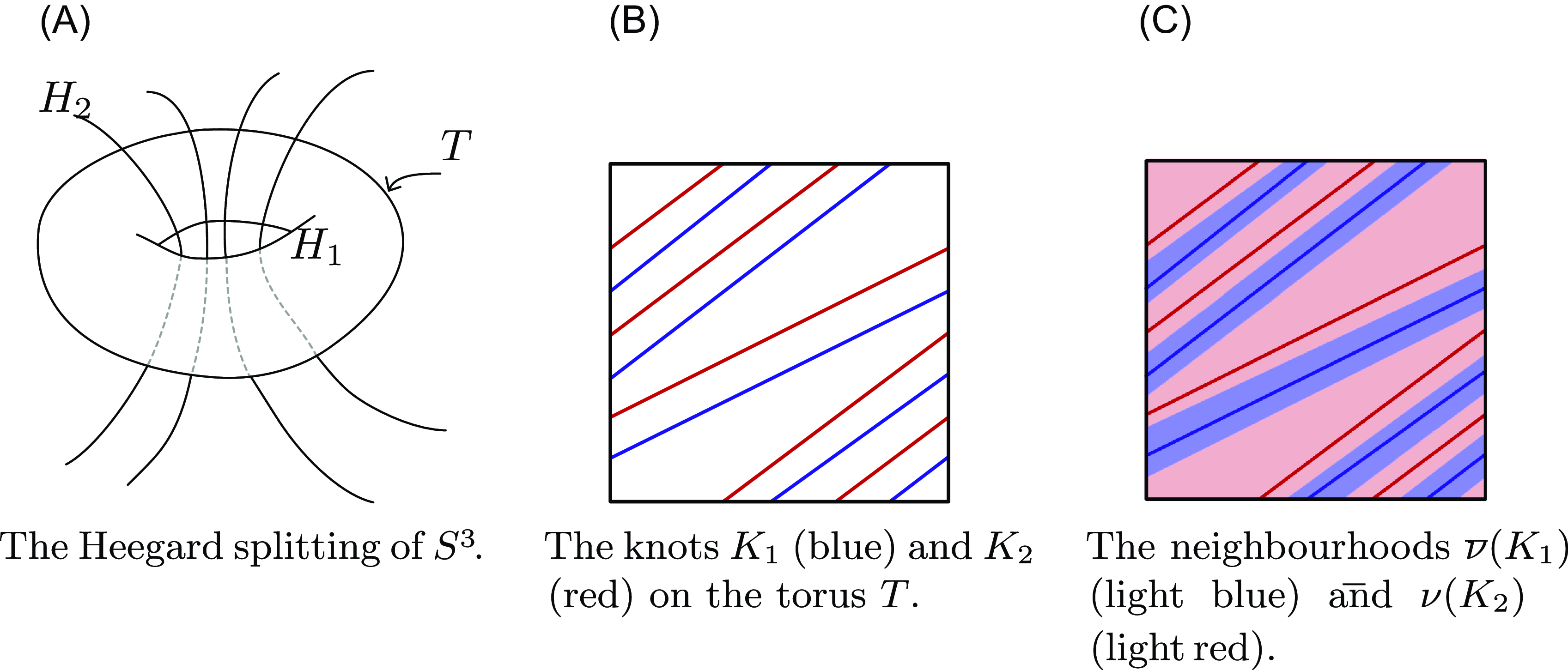
Figure 2. Left frame: the standard genus $1$
Heegaard decomposition of
$1$
Heegaard decomposition of $S^3$
. Central frame: the knots
$S^3$
. Central frame: the knots $K_1$
and
$K_1$
and $K_2$
lying in the Heegaard torus
$K_2$
lying in the Heegaard torus $T$
. Right frame: the neighbourhoods
$T$
. Right frame: the neighbourhoods $\overline{\nu }(K_1)$
and
$\overline{\nu }(K_1)$
and $\overline{\nu }(K_2)$
of
$\overline{\nu }(K_2)$
of $K_1$
and
$K_1$
and $K_2$
that satisfy
$K_2$
that satisfy $T = \overline{\nu }(K_1) \cup \overline{\nu }(K_2)$
and
$T = \overline{\nu }(K_1) \cup \overline{\nu }(K_2)$
and $\overline{\nu }(K_1) \cap \overline{\nu }(K_2) = \partial \overline{\nu }(K_1) = \partial \overline{\nu }(K_2)$
.
$\overline{\nu }(K_1) \cap \overline{\nu }(K_2) = \partial \overline{\nu }(K_1) = \partial \overline{\nu }(K_2)$
.
Construction 7.3.
We describe an explicit handle decomposition for the exterior $X_{T_{2,2k+1}}$
. Our strategy is to first describe
$X_{T_{2,2k+1}}$
. Our strategy is to first describe $X_{T_{2,2k+1}}$
as a union of three solid tori
$X_{T_{2,2k+1}}$
as a union of three solid tori $U_1,U_2$
and
$U_1,U_2$
and $V_1$
. We will then read off a handle decomposition for
$V_1$
. We will then read off a handle decomposition for $X_{T_{2,2k+1}}$
from a handle decomposition of the solid tori.
$X_{T_{2,2k+1}}$
from a handle decomposition of the solid tori.
Consider the standard genus one Heegaard decomposition $S^{3} = H_{1} \cup _{\partial } H_{2}$
with Heegaard surface the torus
$S^{3} = H_{1} \cup _{\partial } H_{2}$
with Heegaard surface the torus $T = H_{1} \cap H_{2}$
. The solid tori
$T = H_{1} \cap H_{2}$
. The solid tori $H_1$
and
$H_1$
and $H_2$
are sketched on the left frame of Figure
2
. Pick two parallel copies
$H_2$
are sketched on the left frame of Figure
2
. Pick two parallel copies $K_1,K_2 \subset T$
of the torus knot
$K_1,K_2 \subset T$
of the torus knot $T_{2,2k+1}$
that lie on the torus
$T_{2,2k+1}$
that lie on the torus $T$
as illustrated in the central frame of Figure
2
. The right-hand side of this figure shows closed neighbourhoods
$T$
as illustrated in the central frame of Figure
2
. The right-hand side of this figure shows closed neighbourhoods $\overline{\nu }(K_1),\overline{\nu }(K_2) \subset T$
that satisfy
$\overline{\nu }(K_1),\overline{\nu }(K_2) \subset T$
that satisfy
 \begin{equation*}T = \overline {\nu }(K_1) \cup \overline {\nu }(K_2) \text { and } \overline {\nu }(K_1) \cap \overline {\nu }(K_2) = \partial \overline {\nu }(K_1) = \partial \overline {\nu }(K_2).\end{equation*}
Shrink the solid tori $H_1 \cong S^1 \times D^2$
and
$H_1 \cong S^1 \times D^2$
and $H_2 \cong S^1 \times D^2$
to obtain half-sized solid tori
$H_2 \cong S^1 \times D^2$
to obtain half-sized solid tori $S^1 \times D^2_{\frac{1}{2}} \cong U_i \subset H_i$
. It follows that
$S^1 \times D^2_{\frac{1}{2}} \cong U_i \subset H_i$
. It follows that $V \;:\!=\; \overline{S^{3} \setminus (U_{1} \cup U_{2})}$
is a tubular neighbourhood of
$V \;:\!=\; \overline{S^{3} \setminus (U_{1} \cup U_{2})}$
is a tubular neighbourhood of $T \subset S^3$
and can be identified with
$T \subset S^3$
and can be identified with $V \cong T \times I \cong (\overline{\nu }(K_1) \cup \overline{\nu }(K_2)) \times I$
. Since we shrank the solid tori
$V \cong T \times I \cong (\overline{\nu }(K_1) \cup \overline{\nu }(K_2)) \times I$
. Since we shrank the solid tori $H_1$
and
$H_1$
and $H_2$
but expanded the torus
$H_2$
but expanded the torus $T=\overline{\nu }(K_1) \cup \overline{\nu }(K_2)$
, we obtain
$T=\overline{\nu }(K_1) \cup \overline{\nu }(K_2)$
, we obtain
 \begin{equation*}S^3=V \cup U_1 \cup U_2=(\overline {\nu }(K_1) \times I) \cup (\overline {\nu }(K_2) \times I) \cup U_1 \cup U_2.\end{equation*}
Recall that $K_2 \subset T$
is a copy of the torus knot
$K_2 \subset T$
is a copy of the torus knot $T_{2,2k+1}$
. Thus when we remove
$T_{2,2k+1}$
. Thus when we remove $\nu (K_2) \cong K_2 \times^{^{^{\;\;\;\circ\!\!\!\!\!\!\!\!}}} {D}^2$
from
$\nu (K_2) \cong K_2 \times^{^{^{\;\;\;\circ\!\!\!\!\!\!\!\!}}} {D}^2$
from $S^3$
, and write
$S^3$
, and write $V_1\;:\!=\;\overline{\nu }(K_1) \times I$
, we obtain the following decomposition of
$V_1\;:\!=\;\overline{\nu }(K_1) \times I$
, we obtain the following decomposition of $X_{T_{2,2k+1}}$
:
$X_{T_{2,2k+1}}$
:
 \begin{equation} X_{T_{2,2k+1}} = U_{1} \cup V_{1} \cup U_{2}. \end{equation}
The intersection $V_1 \cap U_i$
consists a normal push-off of the neighbourhood
$V_1 \cap U_i$
consists a normal push-off of the neighbourhood $\overline{\nu }(K_{1}) \subset T$
into
$\overline{\nu }(K_{1}) \subset T$
into $U_i$
. Put differently,
$U_i$
. Put differently, $V_1 \cap U_i$
is diffeomorphic to
$V_1 \cap U_i$
is diffeomorphic to $\overline{\nu }(K_i')\cong K_i' \times I$
, where
$\overline{\nu }(K_i')\cong K_i' \times I$
, where $K_i' \subset U_i$
is a normal push-off of the knot
$K_i' \subset U_i$
is a normal push-off of the knot $K_i\subset T$
.
$K_i\subset T$
.
The solid tori $U_i$
have handle decompositions with a single
$U_i$
have handle decompositions with a single $0$
-handle and a single
$0$
-handle and a single $1$
-handle, say
$1$
-handle, say $U_{i} = h_{i}^{0} \cup h_{i}^{1}$
, and we will obtain a handle decomposition for
$U_{i} = h_{i}^{0} \cup h_{i}^{1}$
, and we will obtain a handle decomposition for $X_{T_{2,2k+1}}$
by decomposing
$X_{T_{2,2k+1}}$
by decomposing $V_1$
as a union of two
$V_1$
as a union of two $3$
-balls
$3$
-balls $B_1$
and
$B_1$
and $B_2$
and showing that adding
$B_2$
and showing that adding $V_1$
to
$V_1$
to $U_1 \sqcup U_2$
is the same as adding a
$U_1 \sqcup U_2$
is the same as adding a $1$
-handle followed by a
$1$
-handle followed by a $2$
-handle.
$2$
-handle.
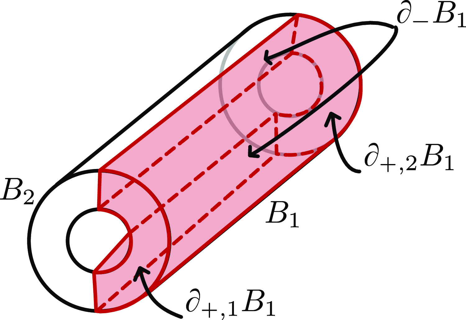
Figure 3. The solid torus $V_1 \cong S^1 \times I^2$
and its decomposition as a union of two
$V_1 \cong S^1 \times I^2$
and its decomposition as a union of two $3$
-balls,
$3$
-balls, $B_1$
(red) and
$B_1$
(red) and $B_2$
(the remaining part of
$B_2$
(the remaining part of $V_{1}$
). The attaching region
$V_{1}$
). The attaching region $\partial _+ B_1=\partial _{+,1} B_{1} \sqcup \partial _{+,2} B_{1}$
of
$\partial _+ B_1=\partial _{+,1} B_{1} \sqcup \partial _{+,2} B_{1}$
of $B_1$
, thought of as a
$B_1$
, thought of as a $1$
-handle, is also shown.
$1$
-handle, is also shown.
Fix a diffeomorphism $\psi \colon S^{1} \times I^{2} \xrightarrow{\cong } V_{1}$
such that
$\psi \colon S^{1} \times I^{2} \xrightarrow{\cong } V_{1}$
such that $N_{1} = V_{1} \cap T = \psi (S^{1} \times I \times \{1/2\})$
, and
$N_{1} = V_{1} \cap T = \psi (S^{1} \times I \times \{1/2\})$
, and $V_{1} \cap U_{i} = \psi (S^{1} \times I \times \{i-1\})$
. Define
$V_{1} \cap U_{i} = \psi (S^{1} \times I \times \{i-1\})$
. Define $B_{1} = \psi ([0,\pi ] \times I^{2}) \subset V_{1}$
and
$B_{1} = \psi ([0,\pi ] \times I^{2}) \subset V_{1}$
and $B_{2} = \psi ([\pi,2 \pi ] \times I^{2}) \subset V_{1}$
. Note that both
$B_{2} = \psi ([\pi,2 \pi ] \times I^{2}) \subset V_{1}$
. Note that both $B_1$
and
$B_1$
and $B_2$
are diffeomorphic to
$B_2$
are diffeomorphic to $3$
-balls and that
$3$
-balls and that $V_1=B_1 \cup B_2$
, as illustrated in Figure
3
. In what follows, we will be thinking of
$V_1=B_1 \cup B_2$
, as illustrated in Figure
3
. In what follows, we will be thinking of $B_1$
as a
$B_1$
as a $3$
-dimensional
$3$
-dimensional $1$
-handle and of
$1$
-handle and of $B_2$
as a
$B_2$
as a $3$
-dimensional
$3$
-dimensional $2$
-handle. The attaching region
$2$
-handle. The attaching region $\partial _+ B_1=\partial _{+,1} B_{1} \sqcup \partial _{+,2} B_{1}$
of
$\partial _+ B_1=\partial _{+,1} B_{1} \sqcup \partial _{+,2} B_{1}$
of $B_1$
can be also be seen in Figure
3
.
$B_1$
can be also be seen in Figure
3
.
-
• When
$V_1$
is glued to
$U_1 \sqcup U_2$
, the
$1$
-handle
$h_{3}^{1}=B_{1}$
is attached to the union
$U_{1} \sqcup U_{2}$
as illustrated in the top frame of Figure
4
. In more detail, we consider the aforementioned normal push offs
$K'_{\!\!1} \subset U_1$
and
$K'_{\!\!2} \subset U_2$
of
$K_1,K_2 \subset T$
, and the attaching regions of
$B_1$
and
$B_2$
are identified with a small
$2$
-disc neighbourhood of an unknotted portion of
$K'_{\!\!1}$
and
$K'_{\!\!2}$
.Figure 4. The space
$Z$
obtained from
$U_1 \sqcup U_2$
by attaching
$B_1$
is diffeomorphic to a genus two handlebody. This top figure shows the torus knots
$K'_{\!\!1} \subset U_1$
and
$K'_{\!\!2} \subset U_2$
, expressed using a symplectic basis for
$\partial U_1$
and
$\partial U_2$
. Taking the connected sum of these knots (as depicted in the bottom figure) leads to the knot
$J$
, which serves as the attaching circle for the attachment of the
$2$
-handle
$B_2$
.The effect of the handle attachment,
$Z \;:\!=\; U_{1} \cup B_{1} \cup U_{2},$
is diffeomorphic to a genus two handlebody and admits
$h_{0}^{1} \cup h_{2}^{0} \cup h_{1}^{1} \cup h_{2}^{1} \cup h_{3}^{1}$
as a handle decomposition. By performing isotopies of handle decompositions of
$U_{1}$
and
$U_{2}$
, we can assume that
$h_{3}^{1}$
cancels geometrically with either
$0$
-handle. Thus, there is a handle decomposition of
$Z$
of the form
where the right-hand side diffeomorphism results from cancelling
\begin{equation*}Z = h_{1}^{0} \cup h_{2}^{0} \cup h_{1}^{1} \cup h_{2}^{1} \cup h_{3}^{1} \cong h_{1}^{0} \cup h_{1}^{1} \cup h_{1}^{2},\end{equation*}
$h_{2}^{0}$
and
$h_{3}^{1} = B_{1}$
.
-
• When
$V_1$
is glued to
$U_1 \sqcup U_2$
, the
$2$
-handle
$h_r^{2}=B_{2}$
is attached to
$Z$
as illustrated in the bottom frame of Figure
4
. In more detail, the
$2$
-handle
$B_2$
is attached to
$Z$
along the curve
$J \subset \partial Z$
given by the connected sum of
$K'_{\!\!1}$
and
$K'_{\!\!2}$
that is also illustrated in the bottom frame of Figure
4
.


As a result, we have obtained a handle decomposition of $X_{T_{2,2k+1}}$
of the form
$X_{T_{2,2k+1}}$
of the form
 \begin{equation*}X_{T_{2,2k+1}} = h^{0}_{1} \cup h^{0}_{2} \cup h^{1}_{1} \cup h^{1}_{2} \cup h^{1}_{3} \cup h^{2}_{r}.\end{equation*}
When we cancel $h_{2}^{0}$
with
$h_{2}^{0}$
with $h_{3}^{1}$
, we obtain a handle decomposition
$h_{3}^{1}$
, we obtain a handle decomposition
 \begin{equation} X_{T_{2,2k+1}} = h^{0} \cup h_{1}^{1} \cup h_{2}^{1} \cup h_{r}^{2}. \end{equation}
Thus, $X_{T_{2,2k+1}}$
can be obtained from the genus two handlebody
$X_{T_{2,2k+1}}$
can be obtained from the genus two handlebody $Z$
by attaching a
$Z$
by attaching a $2$
-handle
$2$
-handle $h_{r}^{2}$
along a simple closed curve representing the element
$h_{r}^{2}$
along a simple closed curve representing the element $\alpha = a^{2k+1} c^{2} b^{2} d^{2k+1}$
where
$\alpha = a^{2k+1} c^{2} b^{2} d^{2k+1}$
where $a,c,b,d$
is a standard basis of
$a,c,b,d$
is a standard basis of $\pi _{1}(\partial Z)$
, with
$\pi _{1}(\partial Z)$
, with $c$
and
$c$
and $d$
representing meridians of
$d$
representing meridians of $Z$
. In particular,
$Z$
. In particular, $\pi _{1}(Z)$
is a rank-two free group generated by
$\pi _{1}(Z)$
is a rank-two free group generated by $a$
and
$a$
and $b$
, and
$b$
, and $J$
, viewed as a curve in
$J$
, viewed as a curve in $Z$
, represents the element
$Z$
, represents the element $a^{2k+1}b^{2}$
, as desired. Observe that there is no framing ambiguity in this case, see [Reference Gompf and Stipsicz18
, Example 4.1.4.(c)].
$a^{2k+1}b^{2}$
, as desired. Observe that there is no framing ambiguity in this case, see [Reference Gompf and Stipsicz18
, Example 4.1.4.(c)].
Construction 7.4.
Now that we have the handle decomposition (7.3) for $X_{T_{2,2k+1}}$
, we can obtain a handle decomposition of the zero-surgery
$X_{T_{2,2k+1}}$
, we can obtain a handle decomposition of the zero-surgery $M_{T_{2,2k+1}}$
. Indeed, to the handle decomposition (7.3) we attach a
$M_{T_{2,2k+1}}$
. Indeed, to the handle decomposition (7.3) we attach a $2$
-handle
$2$
-handle $h_{\lambda }^{2}$
, which annihilates the zero-framed longitude of
$h_{\lambda }^{2}$
, which annihilates the zero-framed longitude of $T_{2,2k+1}$
and a
$T_{2,2k+1}$
and a $3$
-handle
$3$
-handle $h^{3}$
. Consequently, we obtain a handle decomposition of the zero-surgery of the following form
$h^{3}$
. Consequently, we obtain a handle decomposition of the zero-surgery of the following form
 \begin{equation} M_{T_{2,2k+1}} = h^{0} \cup h_{1}^{1} \cup h_{2}^{1} \cup h_{r}^{2} \cup h_{\lambda }^{2} \cup h^{3}. \end{equation}
By construction, this handle decomposition leads to the presentation $G_0$
of
$G_0$
of $\pi _1(M_{T_{2,2k+1}} )$
.
$\pi _1(M_{T_{2,2k+1}} )$
.
Now let us study identities of the presentation $G_{0}$
from (7.1). Following the notation in Section 5.2, let
$G_{0}$
from (7.1). Following the notation in Section 5.2, let $\textbf{x} = \{a,b\}$
be the set of generators of
$\textbf{x} = \{a,b\}$
be the set of generators of $G_{0}$
and let
$G_{0}$
and let $\textbf{r} = \{R = a^{2k+1}b^{2},\lambda = (a^{k}b)^{2k+1}a^{2k+1}(a^{k}b)^{2k+1}\}$
be the set of relations of
$\textbf{r} = \{R = a^{2k+1}b^{2},\lambda = (a^{k}b)^{2k+1}a^{2k+1}(a^{k}b)^{2k+1}\}$
be the set of relations of $G_{0}$
. Denote by
$G_{0}$
. Denote by $F$
the free group on the set
$F$
the free group on the set $\textbf{x}$
and by
$\textbf{x}$
and by $P$
the free group generated by symbols
$P$
the free group generated by symbols $\rho _{r}$
, for
$\rho _{r}$
, for $r \in \textbf{r}$
. By
$r \in \textbf{r}$
. By $N(G_{0})$
we denote the normal subgroup of
$N(G_{0})$
we denote the normal subgroup of $F \ast P$
generated by
$F \ast P$
generated by $P$
. Consider the map
$P$
. Consider the map $\psi \colon F \ast P \to F$
given by the formula
$\psi \colon F \ast P \to F$
given by the formula
 \begin{equation*}\psi (x) = x, \quad \psi (\rho _{r}) = r,\end{equation*}
where $x \in \textbf{x}$
and
$x \in \textbf{x}$
and $r \in \textbf{r}$
. We will denote by the same symbol the restriction of
$r \in \textbf{r}$
. We will denote by the same symbol the restriction of $\psi$
to
$\psi$
to $N(G_{0})$
. Recall that
$N(G_{0})$
. Recall that $I(G_{0}) \;:\!=\; \ker\!(\psi ) \cap N(G_{0})$
and
$I(G_{0}) \;:\!=\; \ker\!(\psi ) \cap N(G_{0})$
and $[[N(G_{0}),N(G_{0})]]_{\psi }$
denote the normal subgroup of
$[[N(G_{0}),N(G_{0})]]_{\psi }$
denote the normal subgroup of $N(G_{0})$
generated by Peiffer commutators, see Definition 5.2.
$N(G_{0})$
generated by Peiffer commutators, see Definition 5.2.
Lemma 7.5.
Set $R = a^{2k+1}b^{2}$
,
$R = a^{2k+1}b^{2}$
, $\lambda = (a^{k}b)^{2k+1}a^{2k+1}(a^{k}b)^{2k+1}$
and
$\lambda = (a^{k}b)^{2k+1}a^{2k+1}(a^{k}b)^{2k+1}$
and $\mu = (a^{k}b)^{-1}$
. The following equality is satisfied in the free group
$\mu = (a^{k}b)^{-1}$
. The following equality is satisfied in the free group $F$
generated by
$F$
generated by $a$
and
$a$
and $b$
:
$b$
:
 \begin{equation*}\mu \lambda \mu ^{-1} \lambda ^{-1} = \left [\mu ^{-2k}a^{k}\right ] R \left [\mu ^{-2k}a^{k}\right ]^{-1} \mu ^{-2k-1} R^{-1} \mu ^{2k+1}.\end{equation*}
Consequently, the presentation (7.1) of $\pi _{1}(M_{T_{2,2k+1}})$
admits the following identity:
$\pi _{1}(M_{T_{2,2k+1}})$
admits the following identity:
 \begin{equation} s = \mu \rho _{2} \mu ^{-1} \rho _{2}^{-1} \mu ^{-2k-1} \rho _{1} \mu ^{2k+1} \left (\mu ^{-2k} a^{k}\right ) \rho _{1}^{-1}\left (\mu ^{-2k}a^{k}\right )^{-1}. \end{equation}
Furthermore, $s$
is a generator of the group of identities
$s$
is a generator of the group of identities $I(G_{0})/ [[N(G_{0}),N(G_{0}))]]_{\psi }$
.
$I(G_{0})/ [[N(G_{0}),N(G_{0}))]]_{\psi }$
.
Proof. The proof of the first assertion is a direct computation:
 \begin{align*} \mu \lambda \mu ^{-1} \lambda ^{-1} &= (a^{k}b)^{2k} a^{3k+1} b a^{-2k-1} (a^{k}b)^{-2k-1} \\[5pt] &= \left [(a^{k}b)^{2k+1} a^{k} \right ] (a^{2k+1}b^{2}) b (b^{-2}a^{-2k-1}) (a^{k}b)^{-2k-1} \\[5pt] &= \left [\mu ^{-2k-1} a^{k} \right ] R \left [\mu ^{-2k-1} a^{k} \right ]^{-1} \left [\mu ^{-2k-1} a^{k} \right ] b \mu ^{2k+1} \mu ^{-2k-1} R^{-1} \mu ^{2k+1} \\[5pt] &= \left [\mu ^{-2k}a^{k}\right ] R \left [\mu ^{-2k}a^{k}\right ]^{-1} \mu ^{-2k-1} R^{-1} \mu ^{2k+1}. \end{align*}
Consequently, $s$
is indeed an identity of the presentation
$s$
is indeed an identity of the presentation $G_{0}$
.
$G_{0}$
.
To prove the last assertion, observe that the handle decomposition from Construction 7.4 admits a single $3$
-handle. Therefore, by Proposition 6.4,
$3$
-handle. Therefore, by Proposition 6.4, $G_{0}$
admits a single identity, let us denote it by
$G_{0}$
admits a single identity, let us denote it by $s_{1}$
, which is unique up to conjugation by elements of
$s_{1}$
, which is unique up to conjugation by elements of $F$
and up to Peiffer commutators. Furthermore, every element of
$F$
and up to Peiffer commutators. Furthermore, every element of $I(G_{0})/ [[N(G_{0}),N(G_{0}))]]_{\psi }$
can be written, modulo Peiffer commutators, as a product of conjugates of
$I(G_{0})/ [[N(G_{0}),N(G_{0}))]]_{\psi }$
can be written, modulo Peiffer commutators, as a product of conjugates of $s_{1}$
by elements of
$s_{1}$
by elements of $F$
.
$F$
.
Remark 7.6.
We came up with the identity $s$
in (7.5) as follows. Since
$s$
in (7.5) as follows. Since $\mu$
and
$\mu$
and $\lambda$
commute in
$\lambda$
commute in $\pi _1(X_{T_{2,2k+1}})$
, the commutator
$\pi _1(X_{T_{2,2k+1}})$
, the commutator $\mu \lambda \mu ^{-1} \lambda ^{-1}$
is expressible as a product of conjugates of the relation
$\mu \lambda \mu ^{-1} \lambda ^{-1}$
is expressible as a product of conjugates of the relation $r$
and its inverse (cf. the first equation in Lemma 7.5). Identities are typically obtained by combining two relations in
$r$
and its inverse (cf. the first equation in Lemma 7.5). Identities are typically obtained by combining two relations in $\pi _1$
, so we then combined the aforementioned relation (specifically, using
$\pi _1$
, so we then combined the aforementioned relation (specifically, using $r$
) with the relation
$r$
) with the relation $\lambda =1$
.
$\lambda =1$
.
Having fixed the handle decomposition of $M_{T_{2,2k+1}}$
, we can describe the handle chain complex
$M_{T_{2,2k+1}}$
, we can describe the handle chain complex $C_{\ast }^{\text{hnd}}(\widetilde{M}_{T_{2,2k+1}})$
as well as the component of the chain homotopy equivalence
$C_{\ast }^{\text{hnd}}(\widetilde{M}_{T_{2,2k+1}})$
as well as the component of the chain homotopy equivalence $\Phi \colon C^{2}_{\text{hnd}}(\widetilde{M}_{T_{2,2k+1}}) \to C_{1}^{\text{hnd}}(\widetilde{M}_{T_{2,2k+1}})$
. For a quick review of the handle chain complex, refer to Section 6.1.
$\Phi \colon C^{2}_{\text{hnd}}(\widetilde{M}_{T_{2,2k+1}}) \to C_{1}^{\text{hnd}}(\widetilde{M}_{T_{2,2k+1}})$
. For a quick review of the handle chain complex, refer to Section 6.1.
Proposition 7.7.
The handle chain complex for the universal cover of the zero-surgery $M_{T_{2,2k+1}}$
is given by the
$M_{T_{2,2k+1}}$
is given by the $\mathbb{Z}[G_0]$
-module chain complex
$\mathbb{Z}[G_0]$
-module chain complex $\mathbb{Z}[G_{0}] \xrightarrow{\partial _{3}} \mathbb{Z}[G_{0}]^{2} \xrightarrow{\partial _{2}} \mathbb{Z}[G_{0}]^{2} \xrightarrow{\partial _{1}} \mathbb{Z}[G_{0}],$
where the differentials are described by the following formulas:
$\mathbb{Z}[G_{0}] \xrightarrow{\partial _{3}} \mathbb{Z}[G_{0}]^{2} \xrightarrow{\partial _{2}} \mathbb{Z}[G_{0}]^{2} \xrightarrow{\partial _{1}} \mathbb{Z}[G_{0}],$
where the differentials are described by the following formulas:
 \begin{align*} \partial _{3} &= \begin{pmatrix} \mu ^{-2k-1}-\mu ^{-2k} \cdot a^{k} & \mu -1 \\[5pt] \end{pmatrix}, \\[5pt] \partial _{2} &= \begin{pmatrix} \dfrac{\partial (a^{2k+1}b^{2})}{\partial a} & \dfrac{\partial (a^{2k+1}b^{2})}{\partial b} \\[12pt] \dfrac{\partial \lambda _{0}}{\partial a} & \dfrac{\partial \lambda _{0}}{\partial b} \\[5pt] \end{pmatrix}, \\[5pt] \partial _{1} &= \begin{pmatrix} a-1 & b-1 \end{pmatrix}^{T}. \end{align*}
Moreover, if $\Phi \colon C^{2}_{\text{hnd}}(\widetilde{M}_{T_{2,2k+1}}) \to C_{1}^{\text{hnd}}(\widetilde{M}_{T_{2,2k+1}})$
denotes the chain map mentioned in (3.2), then
$\Phi \colon C^{2}_{\text{hnd}}(\widetilde{M}_{T_{2,2k+1}}) \to C_{1}^{\text{hnd}}(\widetilde{M}_{T_{2,2k+1}})$
denotes the chain map mentioned in (3.2), then
 \begin{equation} \Phi = \begin{pmatrix} \mu ^{2k+1} \cdot \dfrac{\partial (\mu ^{-2k-1})}{\partial a} - a^{-k} \cdot \mu ^{2k} \cdot \dfrac{\partial (\mu ^{-2k} \cdot a^{k})}{\partial a} & \mu ^{2k+1} \cdot \dfrac{\partial (\mu ^{-2k-1})}{\partial b} - a^{-k} \cdot \mu ^{2k} \cdot \dfrac{\partial (\mu ^{-2k} \cdot a^{k})}{\partial b} \\[12pt] \mu ^{-1} \cdot \dfrac{\partial \mu }{\partial a} & \mu ^{-1} \cdot \dfrac{\partial \mu }{\partial b} \\[5pt] \end{pmatrix}. \end{equation}
Proof. Endow $M_{T_{2,2k+1}}$
with the handle decomposition from (7.4). This handle decomposition admits a single
$M_{T_{2,2k+1}}$
with the handle decomposition from (7.4). This handle decomposition admits a single $3$
-handle. By construction, this handle decomposition induces the presentation
$3$
-handle. By construction, this handle decomposition induces the presentation
 \begin{equation*} \pi _1(M_{T_{2,2k+1}}) \cong \langle a, b \mid a^{2k+1}b^{2}, (a^{k}b)^{2k+1} a^{2k+1} (a^{k}b)^{2k+1}\rangle \end{equation*}
and the identity
 \begin{equation*} R = \mu \rho _{2} \mu ^{-1} \rho _{2}^{-1} \mu ^{-2k-1} \rho _{1} \mu ^{2k+1} \left (\mu ^{-2k} a^{k}\right ) \rho _{1}^{-1}\left (\mu ^{-2k}a^{k}\right )^{-1}.\end{equation*}
Since $M_{T_{2,2k+1}}$
is aspherical [Reference Gabai17, Corollary 5], the result now follows from Proposition 6.6.
$M_{T_{2,2k+1}}$
is aspherical [Reference Gabai17, Corollary 5], the result now follows from Proposition 6.6.
In later computations, we will need the explicit formulas for the $\partial _i$
and, for this reason, we record the following computations which only require Fox calculus:
$\partial _i$
and, for this reason, we record the following computations which only require Fox calculus:
 \begin{align*} \frac{\partial (a^{2k+1}b^{2})}{\partial a} &= 1+a+a^{2}+\cdots +a^{2k}, \\[5pt] \frac{\partial (a^{2k+1}b^{2})}{\partial b} &= a^{2k+1}(1+b), \\[5pt] \frac{\partial \lambda _{0}}{\partial a} &= (1 + (a^{k}b)^{2k+1} a^{2k+1}) \frac{\partial (a^{k}b)^{2k+1}}{\partial a} + (a^{k}b)^{2k+1} (1+a+a^{2}+\cdots +a^{2k}), \\[5pt] \frac{\partial \lambda _{0}}{\partial b} &= (1 + (a^{k}b)^{2k+1} a^{2k+1}) \frac{\partial (a^{k}b)^{2k+1}}{\partial b}, \\[5pt] \frac{\partial (a^{k}b)^{2k+1}}{\partial a} &= (1+a^{k}b+(a^{k}b)^{2}+\cdots +(a^{k}b)^{2k}) (1+a+a^{2}+\cdots +a^{k-1}), \\[5pt] \frac{\partial (a^{k}b)^{2k+1}}{\partial b} &= (1+a^{k}b+(a^{k}b)^{2}+\cdots +(a^{k}b)^{2k}) a^{k}. \end{align*}
7.2. Blanchfield forms twisted by dihedral representations
In this subsection, we use Powell’s algorithm reviewed in Subsection 3.2 to compute metabelian Blanchfield pairings of $T_{2,2k+1}$
.
$T_{2,2k+1}$
.
Use $\Sigma _{2}(T_{2,2k+1})$
to denote the double cover of
$\Sigma _{2}(T_{2,2k+1})$
to denote the double cover of $S^{3}$
branched along
$S^{3}$
branched along $T_{2,2k+1}$
and let
$T_{2,2k+1}$
and let $\xi = \xi _{2k+1}$
be a primitive root of unity of order
$\xi = \xi _{2k+1}$
be a primitive root of unity of order $2k+1$
. Recall from Subsection 3.1 that for every character
$2k+1$
. Recall from Subsection 3.1 that for every character $\chi \colon H_1(\Sigma _{2}(T_{2,2k+1});\;\mathbb{Z}) \to \mathbb{Z}_{2k+1}$
, there is a metabelian representation
$\chi \colon H_1(\Sigma _{2}(T_{2,2k+1});\;\mathbb{Z}) \to \mathbb{Z}_{2k+1}$
, there is a metabelian representation
 \begin{equation*} \alpha (2,\chi ) \colon \pi _1(M_{T_{2,2k+1}}) \to GL_2(\mathbb {C}[t^{\pm 1}]).\end{equation*}
The representation $\alpha (2,\chi )$
can be described quite explicitly. We start by producing generators of the Alexander module of
$\alpha (2,\chi )$
can be described quite explicitly. We start by producing generators of the Alexander module of $T_{2,2k+1}$
. Since the abelianisation map
$T_{2,2k+1}$
. Since the abelianisation map
 \begin{equation*}\operatorname {Ab} \colon G_{0} \cong \pi _1(M_{T_{2,2k+1}})\to \mathbb {Z}\end{equation*}
sends $x_{2k}$
and
$x_{2k}$
and $x_{2k+1}$
to
$x_{2k+1}$
to $1$
, the commutator subgroup
$1$
, the commutator subgroup $G_{0}^{(1)} = [G_{0},G_{0}]$
consists of words in
$G_{0}^{(1)} = [G_{0},G_{0}]$
consists of words in $x_{2k}, x_{2k+1}$
such that the sum of the exponents is zero. In particular,
$x_{2k}, x_{2k+1}$
such that the sum of the exponents is zero. In particular, $x_{2k}x_{2k+1}^{-1} \in G_{0}^{(1)}$
and it is easy to check that
$x_{2k}x_{2k+1}^{-1} \in G_{0}^{(1)}$
and it is easy to check that $G_{0}^{(1)}$
is normally generated by
$G_{0}^{(1)}$
is normally generated by $x_{2k} x_{2k+1}^{-1}$
. Therefore, the image of
$x_{2k} x_{2k+1}^{-1}$
. Therefore, the image of $x_{2k} x_{2k+1}^{-1}$
generates the Alexander module
$x_{2k} x_{2k+1}^{-1}$
generates the Alexander module $H_{1}(M_{K};\;\mathbb{Z}[t^{\pm 1}]) = G_{0}^{(1)}/ G_{0}^{(2)}$
as a
$H_{1}(M_{K};\;\mathbb{Z}[t^{\pm 1}]) = G_{0}^{(1)}/ G_{0}^{(2)}$
as a $\mathbb{Z}[t^{\pm 1}]$
-module. Consider the projection
$\mathbb{Z}[t^{\pm 1}]$
-module. Consider the projection
 \begin{equation*}q \colon G_{0}^{(1)} \to H_{1}(M_{K};\;\mathbb {Z}[t^{\pm 1}]) \stackrel {}{\to } H_{1}(\Sigma _{2}(T_{2,2k+1});\;\mathbb {Z}). \end{equation*}
Since the image of $x_{2k}x_{2k+1}^{-1}$
generates the Alexander module, it follows that
$x_{2k}x_{2k+1}^{-1}$
generates the Alexander module, it follows that $q(x_{2k} x_{2k+1}^{-1})$
generates
$q(x_{2k} x_{2k+1}^{-1})$
generates $H_{1}(\Sigma _{2}(T_{2,2k+1});\;\mathbb{Z})$
. This, in particular, recovers the well-known fact that
$H_{1}(\Sigma _{2}(T_{2,2k+1});\;\mathbb{Z})$
. This, in particular, recovers the well-known fact that $H_1(\Sigma _2(T_{2,2k+1});\;\mathbb{Z})$
is cyclic, and – in fact –
$H_1(\Sigma _2(T_{2,2k+1});\;\mathbb{Z})$
is cyclic, and – in fact – $H_1(\Sigma _2(T_{2,2k+1});\;\mathbb{Z})\cong \mathbb{Z}_{2k+1}$
. As a consequence, the
$H_1(\Sigma _2(T_{2,2k+1});\;\mathbb{Z})\cong \mathbb{Z}_{2k+1}$
. As a consequence, the $2k+1$
characters
$2k+1$
characters $H_{1}(\Sigma _{2}(T_{2,2k+1});\;\mathbb{Z}) \to \mathbb{Z}_{2k+1}$
can be described by imposing that
$H_{1}(\Sigma _{2}(T_{2,2k+1});\;\mathbb{Z}) \to \mathbb{Z}_{2k+1}$
can be described by imposing that
 \begin{equation*}\chi _{\theta } \colon H_{1}(\Sigma _{2}(T_{2,2k+1});\;\mathbb {Z}) \to \mathbb {Z}_{2k+1}\end{equation*}
satisfies $\chi _{\theta }(q(x_{2k} x_{2k+1}^{-1})) = \theta$
for
$\chi _{\theta }(q(x_{2k} x_{2k+1}^{-1})) = \theta$
for $\theta =0,\ldots,2k$
. We shall now use these observations to compute the value of the metabelian representation
$\theta =0,\ldots,2k$
. We shall now use these observations to compute the value of the metabelian representation $\rho _\theta \;:\!=\;\alpha (2,\chi _{\theta })$
on the generators
$\rho _\theta \;:\!=\;\alpha (2,\chi _{\theta })$
on the generators $a$
and
$a$
and $b$
of
$b$
of $G_0$
. Using (4.1), we have
$G_0$
. Using (4.1), we have $\rho _{\theta }(x_{2k} x_{2k+1}^{-1}) = \left (\begin{smallmatrix} \xi ^{\theta } & 0 \\[5pt] 0 & \xi ^{-\theta } \\[5pt] \end{smallmatrix}\right )$
and
$\rho _{\theta }(x_{2k} x_{2k+1}^{-1}) = \left (\begin{smallmatrix} \xi ^{\theta } & 0 \\[5pt] 0 & \xi ^{-\theta } \\[5pt] \end{smallmatrix}\right )$
and $ \rho _{\theta }(x_{2k+1}) =\left (\begin{smallmatrix} 0 & 1 \\[5pt] t & 0 \\[5pt] \end{smallmatrix}\right )\,$
, and we therefore obtain
$ \rho _{\theta }(x_{2k+1}) =\left (\begin{smallmatrix} 0 & 1 \\[5pt] t & 0 \\[5pt] \end{smallmatrix}\right )\,$
, and we therefore obtain
 \begin{equation*}\rho _{\theta }(x_{2k}) = \begin {pmatrix} \xi ^{\theta } & 0 \\[5pt] 0 & \xi ^{-\theta } \\[5pt] \end {pmatrix} \begin {pmatrix} 0 & 1 \\[5pt] t & 0 \\[5pt] \end {pmatrix} = \begin {pmatrix} 0 & \xi ^{\theta } \\[5pt] t \xi ^{-\theta } & 0 \\[5pt] \end {pmatrix}. \end{equation*}
Next, recall from Lemma 7.1 that the generators $a$
and
$a$
and $b$
of
$b$
of $G_0$
are related to the generators
$G_0$
are related to the generators $x_{2k}$
and
$x_{2k}$
and $x_{2k+1}$
by the formulas
$x_{2k+1}$
by the formulas $a=\phi (x_{2k}x_{2k+1})$
and
$a=\phi (x_{2k}x_{2k+1})$
and $b=\phi (x_{2k+1}^{-1}x_{2k}^{-1})^kx_{2k+1}^{-1}$
. As a consequence, the metabelian representation
$b=\phi (x_{2k+1}^{-1}x_{2k}^{-1})^kx_{2k+1}^{-1}$
. As a consequence, the metabelian representation $\rho _\theta$
is entirely described by
$\rho _\theta$
is entirely described by
 \begin{align*} \rho _\theta (a) &= \begin{pmatrix} t\xi ^{-\theta } & 0 \\[5pt] 0 & t \xi ^{\theta } \\[5pt] \end{pmatrix}, \\[5pt] \rho _\theta (b) &= \begin{pmatrix} 0 & t^{-k-1} \xi ^{k \cdot \theta } \\[5pt] t^{-k} \xi ^{-k \cdot \theta } & 0 \\[5pt] \end{pmatrix}. \end{align*}
We can now work towards the description of the module $H^{2}(M_{T_{2,2k+1}};\;\mathbb{C}[t^{\pm 1}]_{\rho _{\theta }}^{2})$
which supports the cohomological Blanchfield pairing. Consider the polynomials
$H^{2}(M_{T_{2,2k+1}};\;\mathbb{C}[t^{\pm 1}]_{\rho _{\theta }}^{2})$
which supports the cohomological Blanchfield pairing. Consider the polynomials $P_{k}(t) = 1+t+t^{2}+\cdots +t^{k}$
and
$P_{k}(t) = 1+t+t^{2}+\cdots +t^{k}$
and $R_\eta (t)=t+t^{-1}-2 \operatorname{Re}(\eta )$
, for
$R_\eta (t)=t+t^{-1}-2 \operatorname{Re}(\eta )$
, for $\eta \in S^1$
. The latter polynomial is the basic polynomial from Subsection 3.1. Furthermore, we shall also need the following symmetric polynomial:
$\eta \in S^1$
. The latter polynomial is the basic polynomial from Subsection 3.1. Furthermore, we shall also need the following symmetric polynomial:
 \begin{equation*}\Delta _{\theta }(t) = t^{-k} \frac {P_{2k}(t)}{\textsf {R}_{\xi ^{\theta }}(t)} = \prod _{\stackrel {i=1}{i \neq \theta }}^{k} \textsf {R}_{\xi ^{i}}(t).\end{equation*}
The next lemma describes the cohomology $\mathbb{C}[t^{\pm 1}]$
-module
$\mathbb{C}[t^{\pm 1}]$
-module $H^{2}(M_{T_{2,2k+1}};\;\mathbb{C}[t^{\pm 1}]_{\rho _{\theta }}^{2})$
.
$H^{2}(M_{T_{2,2k+1}};\;\mathbb{C}[t^{\pm 1}]_{\rho _{\theta }}^{2})$
.
Proposition 7.8.
The module $H^{2}(M_{T_{2,2k+1}};\;\mathbb{C}[t^{\pm 1}]_{\rho _{\theta }}^{2})$
is isomorphic to
$H^{2}(M_{T_{2,2k+1}};\;\mathbb{C}[t^{\pm 1}]_{\rho _{\theta }}^{2})$
is isomorphic to $ \mathbb{C}[t^{\pm 1}]/ (\Delta _{\theta }(t))$
and admits a generator
$ \mathbb{C}[t^{\pm 1}]/ (\Delta _{\theta }(t))$
and admits a generator $[v_2] \in H^{2}(M_{T_{2,2k+1}};\;\mathbb{C}[t^{\pm 1}]_{\rho _{\theta }}^{2})$
such that
$[v_2] \in H^{2}(M_{T_{2,2k+1}};\;\mathbb{C}[t^{\pm 1}]_{\rho _{\theta }}^{2})$
such that
 \begin{equation*}\textrm {Bl}^{\rho _{\theta }}(T_{2,2k+1})([v_2],[v_2]) = \frac {\frac {1}{2}(t^{2k+1} \xi ^{k\theta } - t^{k+1} -t^{k}+\xi ^{(k+1)\theta })(t^{-2k-1}+1)}{t^{-k}P_{2k}(t)}.\end{equation*}
Proof. Since $H^{2}(M_{T_{2,2k+1}};\;\mathbb{C}[t^{\pm 1}]_{\rho _{\theta }}^{2})$
is equal to the quotient
$H^{2}(M_{T_{2,2k+1}};\;\mathbb{C}[t^{\pm 1}]_{\rho _{\theta }}^{2})$
is equal to the quotient $\ker\!({{\partial _3}^{\#T}})/\textrm{im}({{\partial _2}^{\# T}})$
, we first compute
$\ker\!({{\partial _3}^{\#T}})/\textrm{im}({{\partial _2}^{\# T}})$
, we first compute $\ker\!({{\partial _3}^{\#T}})$
, before studying
$\ker\!({{\partial _3}^{\#T}})$
, before studying $\textrm{im}({{\partial _2}^{\#T}})$
. First of all, note that
$\textrm{im}({{\partial _2}^{\#T}})$
. First of all, note that $\rho _{\theta }(\mu ) = \rho _{\theta }(x_{2k+1}) = \left (\begin{smallmatrix} 0 & 1 \\[5pt] t & 0 \end{smallmatrix}\right )\,$
. Using this computation and looking back to the definition of
$\rho _{\theta }(\mu ) = \rho _{\theta }(x_{2k+1}) = \left (\begin{smallmatrix} 0 & 1 \\[5pt] t & 0 \end{smallmatrix}\right )\,$
. Using this computation and looking back to the definition of $\partial _3$
(Proposition 7.7), we deduce that
$\partial _3$
(Proposition 7.7), we deduce that
 \begin{equation*}\rho _{\theta }(\partial _{3}) = \begin {pmatrix} -\xi ^{-k\theta } & t^{-k-1} & -1 & 1 \\[5pt] t^{-k} & -\xi ^{k\theta } & t & -1 \\[5pt] \end {pmatrix}. \end{equation*}
The differential $\rho _{\theta }(\partial _{3})^{\#T}$
has rank two; hence,
$\rho _{\theta }(\partial _{3})^{\#T}$
has rank two; hence, $\ker\!(\rho _{\theta }(\partial _{3})^{\#T})$
is
$\ker\!(\rho _{\theta }(\partial _{3})^{\#T})$
is $2$
-dimensional. In fact, we claim that the kernel of
$2$
-dimensional. In fact, we claim that the kernel of $\rho _{\theta }(\partial _{3})^{\# T}$
is freely generated by
$\rho _{\theta }(\partial _{3})^{\# T}$
is freely generated by
 \begin{align*} v_{1} &= \left (t^{-k}\xi ^{-k\theta }, t^{-2k-1}, \xi ^{-k\theta } P_{2k}(t^{-1}), \xi ^{-k\theta }P_{2k}(t^{-1})\right ), \\[3pt] v_{2} &= \left (0, t^{-1}-1, \xi ^{(k+1)\theta }-t^{k+1}, \xi ^{-k\theta }-t^{k}\right ). \end{align*}
Indeed, it is easy to check that $v_{1} \cdot \rho _{\theta }(\partial _{3})^{\# T} = v_{2} \cdot \rho _{\theta }(\partial _{3})^{\# T} = 0$
and that
$v_{1} \cdot \rho _{\theta }(\partial _{3})^{\# T} = v_{2} \cdot \rho _{\theta }(\partial _{3})^{\# T} = 0$
and that $v_{1}$
and
$v_{1}$
and $v_{2}$
are linearly independent. We now turn to
$v_{2}$
are linearly independent. We now turn to $ \textrm{im}(\rho _{\theta }(\partial _{2})^{\# T})$
. We first compute
$ \textrm{im}(\rho _{\theta }(\partial _{2})^{\# T})$
. We first compute $\rho _{\theta }(\partial _{2})^{\# T}$
, then find a basis for
$\rho _{\theta }(\partial _{2})^{\# T}$
, then find a basis for $C^{1}(M_{T_{2,2k+1}};\;\mathbb{C}[t^{\pm 1}]_{\rho _{\theta }}^{2})$
and finally compute the image. To obtain the first line of
$C^{1}(M_{T_{2,2k+1}};\;\mathbb{C}[t^{\pm 1}]_{\rho _{\theta }}^{2})$
and finally compute the image. To obtain the first line of $\rho _\theta (\partial _2)$
, we compute the Fox derivatives of
$\rho _\theta (\partial _2)$
, we compute the Fox derivatives of $r=a^{2k+1}b^2$
:
$r=a^{2k+1}b^2$
:
 \begin{align*} \rho _{\theta }\left (\frac{\partial r}{\partial a}\right ) &= \begin{pmatrix} P_{2k}(t\xi ^{-\theta }) & 0 \\[3pt] 0 & P_{2k}(t\xi ^{\theta }) \\[3pt] \end{pmatrix}, \\[3pt] \rho _{\theta }\left (\frac{\partial r}{\partial b}\right ) &= \begin{pmatrix} t^{2k+1} & t^{k} \xi ^{k\theta } \\[3pt] t^{k+1} \xi ^{-k\theta } & t^{2k+1} \\[3pt] \end{pmatrix}. \end{align*}
In order to obtain the second line of $\rho _\theta (\partial _{2})$
, we first compute
$\rho _\theta (\partial _{2})$
, we first compute
 \begin{align*} \rho _{\theta }\left (\frac{\partial (a^{k}b)}{\partial a}\right ) &= \begin{pmatrix} P_{k-1}(t\xi ^{-\theta }) & 0 \\[5pt] 0& P_{k-1}(t\xi ^{\theta }) \\[5pt] \end{pmatrix}, \\[5pt] \rho _{\theta }\left (\frac{\partial (a^{k}b)}{\partial b}\right ) &= \begin{pmatrix} t^{k}\xi ^{-k\theta } & 0 \\[5pt] 0 & t^{k}\xi ^{k\theta } \\[5pt] \end{pmatrix}, \\[5pt] \rho _{\theta }\left (\frac{\partial (a^{k}b)^{2k+1}}{\partial a}\right ) &= \begin{pmatrix} P_{k}(t^{-1}) & t^{-1}P_{k-1}(t^{-1}) \\[5pt] P_{k-1}(t^{-1}) & P_{k}(t^{-1}) \end{pmatrix} \cdot \begin{pmatrix} P_{k-1}(t\xi ^{-\theta }) & 0 \\[5pt] 0 & P_{k-1}(t\xi ^{\theta }) \\[5pt] \end{pmatrix} \\[5pt] &= \begin{pmatrix} P_{k}(t^{-1})P_{k-1}(t\xi ^{-\theta }) & t^{-1}P_{k-1}(t^{-1})P_{k-1}(t\xi ^{\theta }) \\[5pt] P_{k-1}(t^{-1})P_{k-1}(t\xi ^{-\theta }) & P_{k}(t^{-1})P_{k-1}(t\xi ^{\theta }) \\[5pt] \end{pmatrix}, \\[5pt] \rho \left (\frac{\partial (a^{k}b)^{2k+1}}{\partial b}\right ) &= \begin{pmatrix} P_{k}(t^{-1}) & t^{-1}P_{k-1}(t^{-1}) \\[5pt] P_{k-1}(t^{-1}) & P_{k}(t^{-1}) \end{pmatrix} \cdot \begin{pmatrix} t^{k}\xi ^{-k\theta } & 0 \\[5pt] 0 & t^{k} \xi ^{k\theta } \\[5pt] \end{pmatrix} \\[5pt] &= \begin{pmatrix} P_{k}(t)\xi ^{-k\theta }& P_{k-1}(t)\xi ^{k\theta } \\[5pt] t P_{k-1}(t) \xi ^{-k\theta } & P_{k}(t) \xi ^{k\theta } \\[5pt] \end{pmatrix}. \end{align*}
As a consequence, the second line of $\partial _2$
is given by
$\partial _2$
is given by
 \begin{align*} \rho _{\theta }\left (\frac{\partial \lambda _{0}}{\partial a}\right ) &= \begin{pmatrix} t^{-k}P_{k-1}(t\xi ^{-\theta })P_{2k}(t) & t^{-k}P_{k-1}(t\xi ^{\theta })P_{2k}(t) + t^{-k-1}P_{2k}(t\xi ^{\theta }) \\[5pt] t^{-k+1}P_{k-1}(t\xi ^{-\theta })P_{2k}(t) + t^{-k}P_{2k}(t\xi ^{-\theta }) & t^{-k}P_{k-1}(t\xi ^{\theta })P_{2k}(t) \\[5pt] \end{pmatrix} \\[5pt] &= \begin{pmatrix} t^{-k}P_{k-1}(t\xi ^{-\theta })P_{2k}(t) & \frac{P_{2k}(t)}{t\xi ^{\theta }-1} (\xi ^{k\theta }-t^{-k-1})\\[5pt] \frac{P_{2k}(t)}{t\xi ^{-\theta }-1}(t\xi ^{-k\theta }-t^{-k}) & t^{-k}P_{k-1}(t\xi ^{\theta })P_{2k}(t) \\[5pt] \end{pmatrix}, \\[5pt] \rho _{\theta }\left (\frac{\partial \lambda _{0}}{\partial b}\right ) &= \begin{pmatrix} \xi ^{-k\theta } P_{2k}(t) & \xi ^{k\theta } P_{2k}(t) \\[5pt] t \xi ^{-k\theta } P_{2k}(t) & \xi ^{k\theta } P_{2k}(t) \\[5pt] \end{pmatrix}. \end{align*}
This completes the first step of our computation of $ \textrm{im}(\rho _{\theta }(\partial _{2})^{\# T})$
. To carry out the second step, consider the following set of vectors of
$ \textrm{im}(\rho _{\theta }(\partial _{2})^{\# T})$
. To carry out the second step, consider the following set of vectors of $C^{1}(M_{T_{2,2k+1}};\;\mathbb{C}[t^{\pm 1}]_{\rho _{\theta }}^{2})$
:
$C^{1}(M_{T_{2,2k+1}};\;\mathbb{C}[t^{\pm 1}]_{\rho _{\theta }}^{2})$
:
 \begin{align} Z_{1} &= \left (\frac{\xi ^{-(k-1)\theta }t^{k+1}}{\xi ^{\theta }-\xi ^{-\theta }}, \frac{\xi ^{-\theta }}{\xi ^{\theta }-\xi ^{-\theta }}, 0, -\frac{t^{2k+1}\xi ^{\theta }P_{2k}(t^{-1}\xi ^{\theta })}{\xi ^{\theta }-\xi ^{-\theta }}\right ), \\[5pt] Z_{2} &= \left ((t^{-1}\xi ^{\theta }-1)\xi ^{-k\theta }t^{k+1}, t^{-1}\xi ^{-\theta }-1, 0, t^{2k+1}-1\right ), \nonumber \\[5pt] Z_{3} &= \left (0, t^{-k-2}\xi ^{(k-1)\theta }-\xi ^{k\theta }t^{-k-1}, 1, -\xi ^{k\theta }t^{-k-1}\right ), \nonumber \\[5pt] Z_{4} &= \left (0,0,0,1\right ) \nonumber. \end{align}
We claim that this collection of vectors yields a basis of $C^{1}(M_{T_{2,2k+1}};\;\mathbb{C}[t^{\pm 1}]_{\rho _{\theta }}^{2})$
. Indeed, if
$C^{1}(M_{T_{2,2k+1}};\;\mathbb{C}[t^{\pm 1}]_{\rho _{\theta }}^{2})$
. Indeed, if $Z$
denotes the matrix whose rows are
$Z$
denotes the matrix whose rows are $Z_{1}, Z_{2}, Z_{3}$
and
$Z_{1}, Z_{2}, Z_{3}$
and $Z_{4}$
, then
$Z_{4}$
, then $\det\!(Z) = -t^{k+1}\xi ^{-k\theta }$
: this determinant can be computed by first expanding along the fourth row and then expanding along the third column. Finally, we carry out the third and last step: using this basis of vectors, we compute the image of
$\det\!(Z) = -t^{k+1}\xi ^{-k\theta }$
: this determinant can be computed by first expanding along the fourth row and then expanding along the third column. Finally, we carry out the third and last step: using this basis of vectors, we compute the image of $\rho _\theta (\partial _2)^{\# T}\,$
by observing that
$\rho _\theta (\partial _2)^{\# T}\,$
by observing that
 \begin{align} Z_{1} \cdot \rho _{\theta }(\partial _{2})^{\# T} &= t^{-k+1} \cdot \Delta _{\theta }(t^{-1}) \cdot v_{2}, \\[5pt] Z_{2} \cdot \rho _{\theta }(\partial _{2})^{\# T} &= 0, \nonumber \\[5pt] Z_{3} \cdot \rho _{\theta }(\partial _{2})^{\# T} &= 0, \nonumber \\[5pt] Z_{4} \cdot \rho _{\theta }(\partial _{2})^{\# T} &= v_{1}. \nonumber \end{align}
We therefore deduce that the twisted homology $\mathbb{C}[t^{\pm 1}]$
-module
$\mathbb{C}[t^{\pm 1}]$
-module $H^{2}(M_{T_{2,2k+1}};\;\mathbb{C}[t^{\pm 1}]_{\rho _{\theta }}^{2})$
is cyclic with order
$H^{2}(M_{T_{2,2k+1}};\;\mathbb{C}[t^{\pm 1}]_{\rho _{\theta }}^{2})$
is cyclic with order $\Delta _{\theta }(t)$
. This concludes the proof of the first assertion of the proposition.
$\Delta _{\theta }(t)$
. This concludes the proof of the first assertion of the proposition.
In order to compute the twisted Blanchfield pairing, we first compute $\rho _\theta (\Phi )$
using (7.6) and then compute the Blanchfield pairing. We start with the calculation of the coefficients of the first line of
$\rho _\theta (\Phi )$
using (7.6) and then compute the Blanchfield pairing. We start with the calculation of the coefficients of the first line of $\rho _\theta (\Phi )$
. Looking back to (7.6), we see that each of the two blocks consists of a difference of two expressions. We compute each of these terms separately. First, note that we have
$\rho _\theta (\Phi )$
. Looking back to (7.6), we see that each of the two blocks consists of a difference of two expressions. We compute each of these terms separately. First, note that we have
 \begin{align*} \rho _{\theta }\left (\mu ^{2k+1} \cdot \frac{\partial \mu ^{-2k-1}}{\partial a}\right ) &= \begin{pmatrix} 0 & t^{k} \\[5pt] t^{k+1} & 0 \\[5pt] \end{pmatrix} \begin{pmatrix} P_{k}(t^{-1})P_{k-1}(t\xi ^{-\theta }) & t^{-1}P_{k-1}(t^{-1})P_{k-1}(t\xi ^{\theta }) \\[5pt] P_{k-1}(t^{-1})P_{k-1}(t\xi ^{-\theta }) & P_{k}(t^{-1})P_{k-1}(t\xi ^{\theta }) \\[5pt] \end{pmatrix} \\[5pt] &= \begin{pmatrix} t^{k}P_{k-1}(t^{-1})P_{k-1}(t\xi ^{-\theta }) & t^{k}P_{k}(t^{-1})P_{k-1}(t\xi ^{\theta }) \\[5pt] t^{k+1}P_{k}(t^{-1})P_{k-1}(t\xi ^{-\theta }) & t^{k}P_{k-1}(t^{-1})P_{k-1}(t\xi ^{\theta }) \\[5pt] \end{pmatrix}, \\[5pt] \rho _{\theta }\left (\mu ^{2k+1} \cdot \frac{\partial \mu ^{-2k-1}}{\partial b}\right ) &= \begin{pmatrix} 0 & t^{k} \\[5pt] t^{k+1} & 0 \\[5pt] \end{pmatrix} \begin{pmatrix} P_{k}(t)\xi ^{-k\theta }& P_{k-1}(t)\xi ^{k\theta } \\[5pt] t P_{k-1}(t) \xi ^{-k\theta } & P_{k}(t) \xi ^{k\theta } \\[5pt] \end{pmatrix} \\[5pt] &= \begin{pmatrix} t^{k+1}\xi ^{-k\theta }P_{k-1}(t) & t^{k} \xi ^{k\theta }P_{k}(t) \\[5pt] t^{k+1} \xi ^{-k\theta }P_{k}(t) & t^{k+1} \xi ^{k\theta }P_{k-1}(t) \\[5pt] \end{pmatrix}. \end{align*}
The computation of the upper left block of $\rho _\theta (\Phi )$
also requires us to compute
$\rho _\theta (\Phi )$
also requires us to compute
 \begin{align*} \frac{\partial (\mu ^{-2k} \cdot a^{k})}{\partial a} &= \frac{\partial{\mu ^{-2k}}}{\partial a} + \mu ^{-2k} \cdot \frac{\partial{a^{k}}}{\partial a} \\[5pt] &= (1 + \mu ^{-1} + \mu ^{-2} + \cdots + \mu ^{-2k+1}) \cdot \frac{\partial (a^{k} b)}{\partial a} + \mu ^{-2k} \cdot (1+a+a^{2}+\cdots +a^{k-1}) \\[5pt] &= (1 + \mu ^{-1}) \cdot (1 + \mu ^{-2} + \cdots (\mu ^{-2})^{k-1}) \cdot \frac{\partial a^{k}b}{\partial a} + \mu ^{-2k} \cdot (1+a+a^{2}+\cdots +a^{k-1}) \end{align*}
 \begin{align*} \rho _{\theta }\left (\frac{\partial (\mu ^{-2k} \cdot a^{k})}{\partial a}\right ) &= \begin{pmatrix} 1 & t^{-1} \\[5pt] 1 & 1 \\[5pt] \end{pmatrix} \cdot \begin{pmatrix} P_{k-1}(t^{-1}) & 0 \\[5pt] 0 & P_{k-1}(t^{-1}) \\[5pt] \end{pmatrix} \cdot \begin{pmatrix} P_{k-1}(t\xi ^{-\theta }) & 0 \\[5pt] 0 & P_{k-1}(t\xi ^{\theta }) \\[5pt] \end{pmatrix} \\[5pt] &+ \begin{pmatrix} t^{-k} & 0 \\[5pt] 0 & t^{-k} \\[5pt] \end{pmatrix} \cdot \begin{pmatrix} P_{k-1}(t\xi ^{-\theta }) & 0 \\[5pt] 0 & p_{k-1}(t\xi ^{\theta }) \\[5pt] \end{pmatrix} \\[5pt] &= \begin{pmatrix} P_{k}(t^{-1}) P_{k-1}(t\xi ^{-\theta }) & t^{-1}P_{k-1}(t^{-1})P_{k-1}(t\xi ^{\theta }) \\[5pt] P_{k-1}(t^{-1}) P_{k-1}(t\xi ^{-\theta }) & P_{k}(t^{-1})P_{k-1}(t\xi ^{\theta })\\[5pt] \end{pmatrix}, \end{align*}
and, similarly, the upper right block of $\rho _\theta (\Phi )$
requires that we compute
$\rho _\theta (\Phi )$
requires that we compute
 \begin{align*} \frac{\partial (\mu ^{-2k} \cdot a^{k})}{\partial b} &= \frac{\partial \mu ^{-2k}}{\partial b} = (1+\mu ^{-1}) \cdot (1+\mu ^{-2}+\cdots +(\mu ^{-2})^{k-1}) \cdot \frac{\partial a^{k}b}{\partial b}, \\[5pt] \rho _{\theta }\left (\frac{\partial (\mu ^{-2k} \cdot a^{k})}{\partial b}\right ) &= \begin{pmatrix} 1 & t^{-1} \\[5pt] 1 & 1 \\[5pt] \end{pmatrix} \cdot \begin{pmatrix} P_{k-1}(t^{-1}) & 0 \\[5pt] 0 & P_{k-1}(t^{-1}) \\[5pt] \end{pmatrix} \cdot \begin{pmatrix} t^{k} \xi ^{-k\theta } & 0 \\[5pt] 0 & t^{k} \xi ^{k\theta } \\[5pt] \end{pmatrix} \\[5pt] &= \begin{pmatrix} t^{k}\xi ^{-k\theta }P_{k-1}(t^{-1}) & t^{k-1} \xi ^{k\theta } P_{k-1}(t^{-1}) \\[5pt] t^{k}\xi ^{-k\theta }P_{k-1}(t^{-1}) & t^{k}\xi ^{k\theta }P_{k-1}(t^{-1}) \end{pmatrix}, \end{align*}
Consequently, using the two above sequences of computations, we have
 \begin{align*} \rho _{\theta }\left (a^{-k} \cdot \mu ^{2k} \cdot \frac{\partial (\mu ^{-2k} \cdot a^{k})}{\partial a}\right ) &= \begin{pmatrix} \xi ^{k\theta } & 0 \\[5pt] 0 & \xi ^{-k\theta } \\[5pt] \end{pmatrix} \begin{pmatrix} P_{k}(t^{-1}) P_{k-1}(t\xi ^{-\theta }) & t^{-1}P_{k-1}(t^{-1})P_{k-1}(t\xi ^{\theta }) \\[5pt] P_{k-1}(t^{-1}) P_{k-1}(t\xi ^{-\theta }) & P_{k}(t^{-1})P_{k-1}(t\xi ^{\theta })\\[5pt] \end{pmatrix} \\[5pt] &= \begin{pmatrix} \xi ^{k\theta } P_{k}(t^{-1})P_{k-1}(t\xi ^{-\theta }) & \xi ^{k\theta }t^{-1}P_{k-1}(t^{-1}) P_{k-1}(t\xi ^{\theta })\\[5pt] \xi ^{-k\theta } P_{k-1}(t^{-1})P_{k-1}(t\xi ^{-\theta }) & \xi ^{-k\theta }P_{k}(t^{-1})P_{k-1}(t\xi ^{\theta }) \\[5pt] \end{pmatrix}, \\[5pt] \rho _{\theta }\left (a^{-k} \cdot \mu ^{2k} \cdot \frac{\partial (\mu ^{-2k} \cdot a^{k})}{\partial b}\right ) &= \begin{pmatrix} \xi ^{k\theta } & 0 \\[5pt] 0 & \xi ^{-k\theta } \\[5pt] \end{pmatrix} \begin{pmatrix} t^{k}\xi ^{-k\theta }P_{k-1}(t^{-1}) & t^{k-1} \xi ^{k\theta } P_{k-1}(t^{-1}) \\[5pt] t^{k}\xi ^{-k\theta }P_{k-1}(t^{-1}) & t^{k}\xi ^{k\theta }P_{k-1}(t^{-1}) \\[5pt] \end{pmatrix} \\[5pt] &= \begin{pmatrix} t^{k}P_{k-1}(t^{-1}) & t^{k-1}\xi ^{2k\theta }P_{k-1}(t^{-1}) \\[5pt] t^{k}\xi ^{-2k\theta }P_{k-1}(t^{-1}) & t^{k}P_{k-1}(t^{-1}) \\[5pt] \end{pmatrix}. \end{align*}
Looking at (7.6), assembling these computations and taking the appropriate differences provides an explicit understanding of the first row of $\rho _\theta (\Phi )$
. Next, we compute entries in the second row of
$\rho _\theta (\Phi )$
. Next, we compute entries in the second row of $\rho _\theta (\Phi )$
:
$\rho _\theta (\Phi )$
:
 \begin{align*} \rho _{\theta }\left (-\mu ^{-1}\frac{\partial \mu }{\partial a}\right ) &= \begin{pmatrix} -P_{k-1}(t\xi ^{-\theta }) & 0 \\[5pt] 0 & -P_{k-1}(t\xi ^{\theta }) \\[5pt] \end{pmatrix}, \\[5pt] \rho _{\theta }\left (-\mu ^{-1}\frac{\partial \mu }{\partial b}\right ) &= \begin{pmatrix} -t^{k} \xi ^{-k\theta } & 0 \\[5pt] 0 & -t^{k}\xi ^{k\theta } \end{pmatrix}. \end{align*}
Finally, using $\rho _\theta (\Phi )$
and (3.3), we can compute the cohomological twisted Blanchfield pairing of
$\rho _\theta (\Phi )$
and (3.3), we can compute the cohomological twisted Blanchfield pairing of $M_{T_{2,2k+1}}$
. In more detail, we know from (3.3) that if
$M_{T_{2,2k+1}}$
. In more detail, we know from (3.3) that if $v \in Z^2(N;\;{\mathbb{F}[t^{\pm 1}]}^d_{\rho _\theta })$
, then
$v \in Z^2(N;\;{\mathbb{F}[t^{\pm 1}]}^d_{\rho _\theta })$
, then
 \begin{equation*}\textrm {Bl}^{\rho _\theta }(T_{2,2k+1})([v],[v])=\frac {1}{s} \left (v \cdot \rho _\theta (\Phi ) \cdot Z^{\# T}\right )^{\# T},\end{equation*}
where $Z \in C^1(N;\;{\mathbb{F}[t^{\pm 1}]}^d_{\rho _\theta })$
satisfies
$Z \in C^1(N;\;{\mathbb{F}[t^{\pm 1}]}^d_{\rho _\theta })$
satisfies $Z\rho _\theta (\partial ^2)=sv$
for some
$Z\rho _\theta (\partial ^2)=sv$
for some $s \in \, \mathbb{C}[t^{\pm 1}] \setminus \lbrace 0 \rbrace$
. In our case, we take
$s \in \, \mathbb{C}[t^{\pm 1}] \setminus \lbrace 0 \rbrace$
. In our case, we take $v=v_2$
and observe that
$v=v_2$
and observe that $ Z=Z_1$
is described in (7.7) and
$ Z=Z_1$
is described in (7.7) and $s=t^{-k+1}\Delta _\theta (t^{-1})=t^{-k+1}\Delta _\theta (t)$
(recall (7.8)). Therefore, we start by computing
$s=t^{-k+1}\Delta _\theta (t^{-1})=t^{-k+1}\Delta _\theta (t)$
(recall (7.8)). Therefore, we start by computing
 \begin{align*} Z_{1} \cdot &\rho _{\theta }(\Phi )^{\# T} \cdot v_{2}^{\# T}=\\[5pt] &= \frac{1}{\xi ^{\theta }-\xi ^{-\theta }} \cdot \left [\xi ^{-(k-1)\theta } t^{k+1} P_{k-1}(t^{-1}\xi ^{\theta })(1-\xi ^{k\theta }t^{k}) + \xi ^{-\theta } P_{k-1}(t^{-1}\xi ^{-\theta }) (1-\xi ^{k\theta }t^{k+1})\right ] -\\[5pt] &- \frac{1}{\xi ^{\theta }-\xi ^{-\theta }}t^{k+1}\xi ^{-(k-1)\theta }(1-\xi ^{k\theta }t^{k})P_{2k}(t^{-1}\xi ^{\theta }) = \\[5pt] &= \frac{1}{\xi ^{\theta }-\xi ^{-\theta }} \cdot \left [\xi ^{-(k-1)\theta } t^{k+1} P_{k-1}(t^{-1}\xi ^{\theta })(1-\xi ^{k\theta }t^{k}) + \xi ^{-\theta } P_{k-1}(t^{-1}\xi ^{-\theta }) (1-\xi ^{k\theta }t^{k+1})\right ] -\\[5pt] &- \frac{1}{\xi ^{\theta }-\xi ^{-\theta }} \cdot t^{k+1}\xi ^{-(k-1)\theta }(1-\xi ^{k\theta }t^{k})\left [P_{k-1}(t^{-1}\xi ^{\theta }) + t^{-k}\xi ^{k\theta }P_{k}(t^{-1}\xi ^{\theta })\right ] = \\[5pt] &= \frac{1}{\xi ^{\theta }-\xi ^{-\theta }}\left [\xi ^{-\theta }P_{k-1}(t^{-1}\xi ^{-\theta })(1-\xi ^{-(k+1)\theta }t^{k+1}) - t \cdot \xi ^{\theta } (1-t\xi ^{\theta }) P_{k-1}(t\xi ^{\theta })P_{k}(t^{-1}\xi ^{\theta })\right ] = \\[5pt] &= \frac{P_{k-1}(t\xi ^{\theta }) P_{k}(t\xi ^{-\theta })}{\xi ^{\theta } - \xi ^{-\theta }} \left [t^{-k+1} \xi ^{-k\theta } (1-t\xi ^{-\theta }) - t^{-k+1}\xi ^{(k+1)\theta }(1-t\xi ^{\theta })\right ] = \\[5pt] &= \xi ^{(k+1)\theta }t^{-k+2}P_{k-1}(t\xi ^{\theta })P_{k}(t\xi ^{-\theta }). \end{align*}
To facilitate computations, we will now arrange that both the numerator and denominator of $\textrm{Bl}^{\rho _\theta }(T_{2,2k+1})$
are symmetric. To that effect, we observe that if
$\textrm{Bl}^{\rho _\theta }(T_{2,2k+1})$
are symmetric. To that effect, we observe that if $b$
is a symmetric polynomial and
$b$
is a symmetric polynomial and $(a/b)^\#=a/b$
in
$(a/b)^\#=a/b$
in $\mathbb{F}(t)/{\mathbb{F}[t^{\pm 1}]}$
, then
$\mathbb{F}(t)/{\mathbb{F}[t^{\pm 1}]}$
, then $\frac{a}{b}=\frac{\frac{1}{2}(a+a^\#)}{b}$
in
$\frac{a}{b}=\frac{\frac{1}{2}(a+a^\#)}{b}$
in $\mathbb{F}(t)/{\mathbb{F}[t^{\pm 1}]}$
. Applying this remark to the symmetric polynomial
$\mathbb{F}(t)/{\mathbb{F}[t^{\pm 1}]}$
. Applying this remark to the symmetric polynomial $b=\Delta _\theta (t)$
, using
$b=\Delta _\theta (t)$
, using $\textrm{Bl}^{\rho _\theta }$
as a shorthand for
$\textrm{Bl}^{\rho _\theta }$
as a shorthand for $\textrm{Bl}^{\rho _\theta }(T_{2,2k+1})$
and recalling from above that
$\textrm{Bl}^{\rho _\theta }(T_{2,2k+1})$
and recalling from above that $\textrm{Bl}^{\rho _\theta }([v_2],[v_2])=\frac{1}{s}Z_1 \cdot \rho _\theta (\Phi )^{\#T} \cdot v_2^{\#T}$
with
$\textrm{Bl}^{\rho _\theta }([v_2],[v_2])=\frac{1}{s}Z_1 \cdot \rho _\theta (\Phi )^{\#T} \cdot v_2^{\#T}$
with $s=t^{-k+1}\Delta _\theta (t)$
, we obtain
$s=t^{-k+1}\Delta _\theta (t)$
, we obtain
 \begin{align*} \textrm{Bl}^{\rho _\theta }([v_{2}],[v_{2}]) &= \frac{\frac{1}{2}\xi ^{(k+1)\theta }t P_{k-1}(t\xi ^{\theta })P_{k}(t\xi ^{-\theta })}{\Delta _{\theta }(t)} + \frac{\frac{1}{2}\xi ^{-(k+1)\theta }t^{-1}P_{k-1}(t^{-1}\xi ^{-\theta })P_{k}(t^{-1}\xi ^{\theta })}{\Delta _{\theta }(t)} \\[5pt] &= \frac{\frac{1}{2}\xi ^{(k+1)\theta }t P_{k-1}(t\xi ^{\theta })P_{k}(t\xi ^{-\theta })(t^{-2k-1}+1)}{\Delta _{\theta }(t)} \\[5pt] &= \frac{\frac{1}{2}(t^{2k+1} \xi ^{k\theta } - t^{k+1} -t^{k}+\xi ^{(k+1)\theta })(t^{-2k-1}+1)}{t^{-k}P_{2k}(t)}. \end{align*}
This concludes the computation of the twisted Blanchfield pairing on the generator of the twisted cohomology $\mathbb{C}[t^{\pm 1}]$
-module
$\mathbb{C}[t^{\pm 1}]$
-module $H^{2}(M_{T_{2,2k+1}};\;\mathbb{C}[t^{\pm 1}]_{\rho _{\theta }}^{2})$
and thus the proof of the proposition.
$H^{2}(M_{T_{2,2k+1}};\;\mathbb{C}[t^{\pm 1}]_{\rho _{\theta }}^{2})$
and thus the proof of the proposition.
7.3. The isometry type of
$\textrm{Bl}^{\rho _{\theta }}(T_{2,2k+1})$

The aim of this subsection is to determine the isometry type of the twisted Blanchfield forms $\textrm{Bl}^{\rho _\theta }(T_{2,2k+1})$
, where
$\textrm{Bl}^{\rho _\theta }(T_{2,2k+1})$
, where $\rho _\theta =\alpha (2,\chi _\theta )$
. The following proposition (which is Theorem 1.3 from the introduction) implicitly contains the values of the twisted signature jumps
$\rho _\theta =\alpha (2,\chi _\theta )$
. The following proposition (which is Theorem 1.3 from the introduction) implicitly contains the values of the twisted signature jumps $\delta \sigma _{T_{2,2k+1},\rho _\theta } \colon S^1 \to \mathbb{Z}$
.
$\delta \sigma _{T_{2,2k+1},\rho _\theta } \colon S^1 \to \mathbb{Z}$
.
Theorem 7.9.
Set $\xi = \exp \left (\frac{2 \pi i}{2k+1}\right )$
. For any
$\xi = \exp \left (\frac{2 \pi i}{2k+1}\right )$
. For any $k\gt 0$
and
$k\gt 0$
and $1 \leq \theta \leq k$
, there exists an isometry
$1 \leq \theta \leq k$
, there exists an isometry
 \begin{align*} \textrm{Bl}^{\rho _{\theta }}(T_{2,2k+1}) \cong \lambda _{\theta }^{even} \oplus \lambda _{\theta }^{odd}, \end{align*}
where the linking forms $\lambda _{\theta }^{even}$
and
$\lambda _{\theta }^{even}$
and $\lambda _{\theta }^{odd}$
are as follows:
$\lambda _{\theta }^{odd}$
are as follows:
 \begin{align*} \lambda _{\theta }^{odd} &= \bigoplus _{\stackrel{1 \leq e \leq k}{2 \nmid \theta + e}} \left (\mathfrak{e}(1,1, \xi ^{e},\mathbb{C}) \oplus \mathfrak{e}(1,-1,\xi ^{-e},\mathbb{C})\right ), \end{align*}
and
 \begin{align*} \lambda _{\theta }^{even} &= \bigoplus _{\stackrel{1 \leq e \lt \theta }{2 \mid \theta +e}}\left (\mathfrak{e}(1,1,\xi ^{e}, \mathbb{C}) \oplus \mathfrak{e}(1,-1,\xi ^{-e},\mathbb{C})\right ) \oplus \\[5pt] &\bigoplus _{\stackrel{\theta \lt e \leq k}{2 \mid \theta +e}}\left (\mathfrak{e}(1,-1,\xi ^{e}, \mathbb{C}) \oplus \mathfrak{e}(1,1,\xi ^{-e},\mathbb{C})\right ). \end{align*}
Proof. Using Proposition 7.8, we can choose a generator $x$
of the cyclic module
$x$
of the cyclic module $H^{2}(M_{T_{2,2k+1}};\;\mathbb{C}[t^{\pm 1}]_{\rho _{\theta }}^{2})$
so that
$H^{2}(M_{T_{2,2k+1}};\;\mathbb{C}[t^{\pm 1}]_{\rho _{\theta }}^{2})$
so that $\textrm{Bl}^{\rho _{\theta }}(T_{2,2k+1})(x,x) =F(t)$
, where
$\textrm{Bl}^{\rho _{\theta }}(T_{2,2k+1})(x,x) =F(t)$
, where
 \begin{equation*}F(t) = \frac {\frac {1}{2}(t^{2k+1} \xi ^{k\theta } - t^{k+1} -t^{k}+\xi ^{(k+1)\theta })(t^{-2k-1} + 1)}{t^{-k}P_{2k}(t)}.\end{equation*}
Since $\Delta _\theta (t)=\prod _{\stackrel{e=1}{e \neq \theta }}^{k} \textsf{R}_{\xi ^{e}}(t)$
, we know that the isometry type of
$\Delta _\theta (t)=\prod _{\stackrel{e=1}{e \neq \theta }}^{k} \textsf{R}_{\xi ^{e}}(t)$
, we know that the isometry type of $\textrm{Bl}^{\rho _{\theta }}(T_{2,2k+1})$
will involve a direct sum of the basic pairings
$\textrm{Bl}^{\rho _{\theta }}(T_{2,2k+1})$
will involve a direct sum of the basic pairings $ \mathfrak{e}(1,0,\pm 1,\xi ^{e},\mathbb{C})$
. In order to determine the correct signs, and prove the theorem, we will apply the procedure described in Subsection 2.2. The aforementioned signs depend on whether
$ \mathfrak{e}(1,0,\pm 1,\xi ^{e},\mathbb{C})$
. In order to determine the correct signs, and prove the theorem, we will apply the procedure described in Subsection 2.2. The aforementioned signs depend on whether $F(t)(t-\xi ^e)$
is
$F(t)(t-\xi ^e)$
is $\xi ^{e}$
-positive or
$\xi ^{e}$
-positive or $\xi ^{e}$
-negative, for
$\xi ^{e}$
-negative, for $1 \leq e \leq 2k$
and
$1 \leq e \leq 2k$
and $e \neq \theta, 2k+1-\theta$
. Notice that
$e \neq \theta, 2k+1-\theta$
. Notice that $F(t) = \frac{G(t)}{H_{e}(t)} \cdot \frac{1}{\textsf{R}_{\xi ^{e}}(t)}$
, where, for
$F(t) = \frac{G(t)}{H_{e}(t)} \cdot \frac{1}{\textsf{R}_{\xi ^{e}}(t)}$
, where, for $1 \leq e \leq 2k$
, we set
$1 \leq e \leq 2k$
, we set
 \begin{align*} G(t) &= \frac{1}{2}(t^{2k+1} \xi ^{k\theta } - t^{k+1} -t^{k}+\xi ^{(k+1)\theta })(t^{-2k-1} + 1), \\[5pt] H_{e}(t) &= \frac{t^{-k}P_{2k}(t)}{\textsf{R}_{\xi ^{e}}(t)} = \prod _{\stackrel{i=1}{i \neq e}}^{k} \textsf{R}_{\xi ^{i}}(t). \end{align*}
Reformulating, the theorem will immediately follow once we determine the $e$
for which the following function is
$e$
for which the following function is $\xi ^e$
-positive or
$\xi ^e$
-positive or $\xi ^e$
-negative:
$\xi ^e$
-negative:
 \begin{equation} F(t) \cdot (t-\xi ^{e}) = (-1)^{\theta +e}\left [(-1)^{\theta +1}G(t)\right ] \cdot \left [\frac{(-1)^{e-1}}{H_{e}(t)(1-t^{-1}\xi ^{-e})}\right ]. \end{equation}
In Lemma 7.10 below, we show that $\frac{(-1)^{e-1}}{H_{e}(t)(1-t^{-1}\xi ^{-e})}$
is
$\frac{(-1)^{e-1}}{H_{e}(t)(1-t^{-1}\xi ^{-e})}$
is $\xi ^e$
-positive, while in Lemma 7.11, we study the sign of
$\xi ^e$
-positive, while in Lemma 7.11, we study the sign of $(-1)^{\theta +1}G(\xi ^e)$
.
$(-1)^{\theta +1}G(\xi ^e)$
.
Lemma 7.10.
For any $1 \leq e \leq 2k$
, the following function is
$1 \leq e \leq 2k$
, the following function is $\xi ^{e}$
-positive:
$\xi ^{e}$
-positive:
 \begin{equation*}\frac {(-1)^{e-1}}{H_{e}(t)(1-t^{-1}\xi ^{-e})}.\end{equation*}
Proof. Notice that $\frac{1}{1-t^{-1}\xi ^{-e}}$
is
$\frac{1}{1-t^{-1}\xi ^{-e}}$
is $\xi ^{e}$
-positive if
$\xi ^{e}$
-positive if $1 \leq e \leq k$
and
$1 \leq e \leq k$
and $\xi ^{e}$
-negative if
$\xi ^{e}$
-negative if $k+1 \leq e \leq 2k$
. As a consequence, the lemma boils down to determining the sign of
$k+1 \leq e \leq 2k$
. As a consequence, the lemma boils down to determining the sign of $(-1)^{e-1}H_e(\xi ^e)$
. We first check this when
$(-1)^{e-1}H_e(\xi ^e)$
. We first check this when $1 \leq e \leq k$
. For any
$1 \leq e \leq k$
. For any $1 \leq i \leq k$
such that
$1 \leq i \leq k$
such that $e \neq i$
, we have
$e \neq i$
, we have
 \begin{equation*}\textsf {R}_{\xi ^{i}}(\xi ^{e}) = 2\textrm {Re}(\xi ^{e}) - 2 \textrm {Re}(\xi ^{i}) \begin {cases} \gt 0 & \text {if } e\lt i, \\[5pt] \lt 0 & \text {if } e\gt i. \\[5pt] \end {cases} \end{equation*}
Combining these inequalities with the definition of $H_e(t)$
, we obtain
$H_e(t)$
, we obtain
 \begin{equation*}(-1)^{e-1}H_{e}(\xi ^{e}) = \underbrace {(-1)^{e-1}\prod _{i=1}^{e-1}\textsf {R}_{\xi ^{i}}(\xi ^{e})}_{\gt 0} \cdot \underbrace {\prod _{i=e+1}^{k}\textsf {R}_{\xi ^{i}}(\xi ^{e})}_{\gt 0}\gt 0.\end{equation*}
The case $k+1 \leq e \leq 2k$
can be reduced to the previous one. Indeed, notice that
$k+1 \leq e \leq 2k$
can be reduced to the previous one. Indeed, notice that $H_{e}(t) = H_{2k+1-e}(t)$
and
$H_{e}(t) = H_{2k+1-e}(t)$
and $\textsf{R}_{\xi ^{i}}(\xi ^{e}) = \textsf{R}_{\xi ^{i}}(\xi ^{2k+1-e})$
, because
$\textsf{R}_{\xi ^{i}}(\xi ^{e}) = \textsf{R}_{\xi ^{i}}(\xi ^{2k+1-e})$
, because $\textsf{R}_{\xi ^{i}}(t)$
is a real polynomial. This implies that
$\textsf{R}_{\xi ^{i}}(t)$
is a real polynomial. This implies that
 \begin{equation*}(-1)^{e-1}H_{e}(\xi ^{e}) = (-1)^{2k+1-e}H_{2k+1-e}(\xi ^{2k+1-e})\lt 0.\end{equation*}
This concludes the proof of the lemma.
Let us now study the sign of the numerator of (7.9). Notice first that for $1 \leq e \leq k$
, we have
$1 \leq e \leq k$
, we have
 \begin{equation*}G(\xi ^{e}) = G(\xi ^{-e}) = G(\xi ^{2k+1-e}),\end{equation*}
and it is therefore sufficient to determine the sign of $G(\xi ^{e})$
for
$G(\xi ^{e})$
for $1 \leq e \leq k$
.
$1 \leq e \leq k$
.
Lemma 7.11.
For $1 \leq e \leq k$
such that
$1 \leq e \leq k$
such that $e \neq \theta$
, we have
$e \neq \theta$
, we have
 \begin{equation*}(-1)^{\theta +1}G(\xi ^{e}) \begin {cases} \gt 0, & \text { if } 1 \leq e \lt \theta \leq k \text { and } 2 \mid \theta + e, \\[5pt] \lt 0, & \text { if } 1 \leq \theta \lt e \leq k \text { and } 2 \mid \theta +e, \\[5pt] \lt 0, & \text { if } 2 \nmid \theta +e. \end {cases} \end{equation*}
Proof. Using successively the definition of $G(t)$
, the fact that
$G(t)$
, the fact that $\xi =\operatorname{exp}\!(\frac{2\pi i}{2k+1})$
and the identities
$\xi =\operatorname{exp}\!(\frac{2\pi i}{2k+1})$
and the identities
 \begin{equation*}\cos\!(x) - \cos\!(y) = -2 \sin\!\left (\frac {x+y}{2}\right ) \sin\!\left (\frac {x-y}{2}\right ),\end{equation*}
we obtain the following equality:
 \begin{align*} G(\xi ^{e}) &= 2 (\textrm{Re}(\xi ^{k\theta })-\textrm{Re}(\xi ^{ke})) \\[5pt] &= 2 \left (\cos\! \left (\frac{2\pi k\theta }{2k+1}\right ) - \cos\! \left (\frac{2\pi ke}{2k+1}\right )\right ) \\[5pt] &= -4 \sin\! \left (\frac{\pi k (\theta +e)}{2k+1}\right ) \sin\! \left (\frac{\pi k(\theta -e)}{2k+1}\right ) \\[5pt] &= -4 \sin\! \left (\frac{(\theta +e)\pi }{2} - \frac{(\theta +e)\pi }{4k+2}\right ) \sin\! \left (\frac{(\theta -e)\pi }{2}-\frac{(\theta -e)\pi }{4k+2}\right ) = (\!\ast\!). \end{align*}
As a consequence, we consider two cases depending on the parity of $\theta + e$
. First, suppose that
$\theta + e$
. First, suppose that $\theta +e$
is even. Using the identity
$\theta +e$
is even. Using the identity $\sin\! (y+n\pi )=(-1)^{n}\sin\! (y)$
, we deduce that previous expression becomes
$\sin\! (y+n\pi )=(-1)^{n}\sin\! (y)$
, we deduce that previous expression becomes
 \begin{align*} (\!\ast\!) &= 4(-1)^{\theta +1}\sin\! \left (\frac{(\theta +e)\pi }{4k+2}\right ) \sin\! \left (\frac{(\theta -e)\pi }{4k+2}\right ). \end{align*}
Since $\sin\! \left (\frac{(\theta +e)\pi }{4k+2}\right )\gt 0$
and
$\sin\! \left (\frac{(\theta +e)\pi }{4k+2}\right )\gt 0$
and $\sin\! \left (\frac{(\theta -e)\pi }{4k+2}\right )\gt 0$
if
$\sin\! \left (\frac{(\theta -e)\pi }{4k+2}\right )\gt 0$
if $\theta \gt e$
, we deduce that for
$\theta \gt e$
, we deduce that for $\theta +e$
even
$\theta +e$
even
 \begin{equation*}(-1)^{\theta +1}(\!\ast\!) \begin {cases} \gt 0, & 1 \leq e \lt \theta \leq k, \\[5pt] \lt 0, & 1 \leq \theta \lt e \leq k. \\[5pt] \end {cases} \end{equation*}
Next, we suppose that $\theta +e$
is odd. Using the identities
$\theta +e$
is odd. Using the identities $\sin\! (y+\pi n) = (-1)^{n} \sin\! (y)$
and
$\sin\! (y+\pi n) = (-1)^{n} \sin\! (y)$
and $\sin\! (y + \pi/2) = \cos\! (y)$
, we obtain
$\sin\! (y + \pi/2) = \cos\! (y)$
, we obtain
 \begin{align*} (\!\ast\!) &= 4(-1)^{\theta }\cos\! \left (\frac{(\theta +e)\pi }{4k+2}\right ) \cos\! \left (\frac{(\theta -e)\pi }{4k+2}\right ). \end{align*}
Since $1 \leq e \leq k$
, we have
$1 \leq e \leq k$
, we have $\cos\! \left (\frac{(\theta +e)\pi }{4k+2}\right )\gt 0$
and
$\cos\! \left (\frac{(\theta +e)\pi }{4k+2}\right )\gt 0$
and $\cos\! \left (\frac{(\theta -e)\pi }{4k+2}\right )\gt 0$
. Consequently, if
$\cos\! \left (\frac{(\theta -e)\pi }{4k+2}\right )\gt 0$
. Consequently, if $\theta +e$
is odd,
$\theta +e$
is odd, $(-1)^{\theta +1}$ $(\!\ast\!)\lt 0$
. This concludes the proof of the lemma.
$(\!\ast\!)\lt 0$
. This concludes the proof of the lemma.
The proof of Theorem 7.9 is now concluded by using Lemmas 7.10 and 7.11 as well as (7.9) and the remarks which were made at the beginning of the proof.
8. Obstructing the sliceness of algebraic knots
The goal of this section is to illustrate how the combination of Theorem 7.9 and the satellite formula from Theorem 4.3 can be used to obstruct certain algebraic knots from being slice. For concreteness, we focus on the knot $T_{2,3;2,13} \# T_{2,15} \# -T_{2,3;2,15} \# -T_{2,13}$
, an example that was previously considered by Hedden, Kirk and Livingston [Reference Hedden, Kirk and Livingston20].
$T_{2,3;2,13} \# T_{2,15} \# -T_{2,3;2,15} \# -T_{2,13}$
, an example that was previously considered by Hedden, Kirk and Livingston [Reference Hedden, Kirk and Livingston20].
Throughout this section, for an integer $\ell \gt 0$
we set
$\ell \gt 0$
we set $\xi _{\ell } = \exp \left (2\pi i/\ell \right )$
.
$\xi _{\ell } = \exp \left (2\pi i/\ell \right )$
.
8.1. Characters on covers of cable knots
Given a knot $K$
and an odd integer
$K$
and an odd integer $d$
, use
$d$
, use $K_{2,d}$
to denote its
$K_{2,d}$
to denote its $(2,d)$
-cable. In other words,
$(2,d)$
-cable. In other words, $K_{2,d}$
is the satellite knot with pattern the
$K_{2,d}$
is the satellite knot with pattern the $(2,d)$
torus knot
$(2,d)$
torus knot $T_{2,d}$
, companion
$T_{2,d}$
, companion $K$
and infection curve
$K$
and infection curve $\eta = a$
(using the notation from Section 7.1) depicted in Figure 1.
$\eta = a$
(using the notation from Section 7.1) depicted in Figure 1.
The preimage of $\eta$
in the
$\eta$
in the $2$
-fold branched cover
$2$
-fold branched cover $\Sigma _2(T_{2,d})$
consists of two curves
$\Sigma _2(T_{2,d})$
consists of two curves $\widetilde{\eta }_1,\widetilde{\eta }_2$
. Denote by
$\widetilde{\eta }_1,\widetilde{\eta }_2$
. Denote by $\mu _\eta$
and
$\mu _\eta$
and $\lambda _\eta$
the meridian and longitude of
$\lambda _\eta$
the meridian and longitude of $\eta$
and write
$\eta$
and write $\widetilde{\mu }_i$
and
$\widetilde{\mu }_i$
and $\widetilde{\lambda }_i$
for some meridian-longitude pair of the boundary of the tubular neighbourhood of
$\widetilde{\lambda }_i$
for some meridian-longitude pair of the boundary of the tubular neighbourhood of $\widetilde{U}_i \subset \Sigma _2(T_{2,d})$
for
$\widetilde{U}_i \subset \Sigma _2(T_{2,d})$
for $i=1,2$
. Note that
$i=1,2$
. Note that $\widetilde{\mu }_1$
and
$\widetilde{\mu }_1$
and $\widetilde{\mu }_2$
vanish in
$\widetilde{\mu }_2$
vanish in $H_1(\Sigma _2(T_{2,d});\;\mathbb{Z})=\mathbb{Z}_d$
, while the lift
$H_1(\Sigma _2(T_{2,d});\;\mathbb{Z})=\mathbb{Z}_d$
, while the lift $\widetilde{\lambda }_1$
generates
$\widetilde{\lambda }_1$
generates $H_1(\Sigma _2(T_{2,d});\;\mathbb{Z})$
and
$H_1(\Sigma _2(T_{2,d});\;\mathbb{Z})$
and $\widetilde{\lambda }_2=-\widetilde{\lambda }_1$
in
$\widetilde{\lambda }_2=-\widetilde{\lambda }_1$
in $H_1(\Sigma _2(T_{2,d});\;\mathbb{Z})$
. The following topological result is proved in [Reference Hedden, Kirk and Livingston20, Section 2].
$H_1(\Sigma _2(T_{2,d});\;\mathbb{Z})$
. The following topological result is proved in [Reference Hedden, Kirk and Livingston20, Section 2].
Proposition 8.1.
Let $\ell$
be an odd prime. To any character
$\ell$
be an odd prime. To any character $\chi \colon H_1(\Sigma _2(K_{2,d});\;\mathbb{Z}) \to \mathbb{Z}_{\ell }$
, one can associate an integer
$\chi \colon H_1(\Sigma _2(K_{2,d});\;\mathbb{Z}) \to \mathbb{Z}_{\ell }$
, one can associate an integer $\theta$
modulo
$\theta$
modulo $\ell$
by the condition
$\ell$
by the condition $\chi (\widetilde{\lambda }_1)=\xi _{\ell }^{\theta }$
. This character is denoted
$\chi (\widetilde{\lambda }_1)=\xi _{\ell }^{\theta }$
. This character is denoted $\chi _{\theta }$
. In particular, this sets up a bijective correspondence between
$\chi _{\theta }$
. In particular, this sets up a bijective correspondence between $\mathbb{Z}_{\ell }$
-valued characters on
$\mathbb{Z}_{\ell }$
-valued characters on $H_1(\Sigma _2(K_{2,d});\;\mathbb{Z})$
and on
$H_1(\Sigma _2(K_{2,d});\;\mathbb{Z})$
and on $ H_1(\Sigma _2(T_{2,d});\;\mathbb{Z})$
.
$ H_1(\Sigma _2(T_{2,d});\;\mathbb{Z})$
.
Given an oriented knot $K$
, as is customary in knot concordance, we use
$K$
, as is customary in knot concordance, we use $-K$
to denote the mirror image of
$-K$
to denote the mirror image of $K$
with the reversed orientation, that is,
$K$
with the reversed orientation, that is, $-K=\overline{K}^r$
. The next remark, which follows [Reference Hedden, Kirk and Livingston20, Lemma 3.2], describes the characters on
$-K=\overline{K}^r$
. The next remark, which follows [Reference Hedden, Kirk and Livingston20, Lemma 3.2], describes the characters on $H_1(\Sigma _2(-K);\;\mathbb{Z})$
.
$H_1(\Sigma _2(-K);\;\mathbb{Z})$
.
Remark 8.2.
By definition of the reverse mirror image, there is an orientation reversing homeomorphism $h \colon \Sigma _2(K) \to \Sigma _2(-K)$
, and, from now on, it will be understood that we identify the characters on
$h \colon \Sigma _2(K) \to \Sigma _2(-K)$
, and, from now on, it will be understood that we identify the characters on $H_1(\Sigma _2(K);\;\mathbb{Z})$
and with those on
$H_1(\Sigma _2(K);\;\mathbb{Z})$
and with those on $H_1(\Sigma _2(-K);\;\mathbb{Z})$
via this homeomorphism. With this convention, the same proof as in [
Reference Borodzik, Conway and Politarczyk1, Proposition 3.4] shows that
$H_1(\Sigma _2(-K);\;\mathbb{Z})$
via this homeomorphism. With this convention, the same proof as in [
Reference Borodzik, Conway and Politarczyk1, Proposition 3.4] shows that $\textrm{Bl}_{\alpha (2,\chi )}(-K)=-\textrm{Bl}_{\alpha (2,\chi )}(K)$
. Note however that the character we fixed on
$\textrm{Bl}_{\alpha (2,\chi )}(-K)=-\textrm{Bl}_{\alpha (2,\chi )}(K)$
. Note however that the character we fixed on $-K$
is not the one obtained by combining the second and third items of [
Reference Borodzik, Conway and Politarczyk1, Proposition 3.4].
$-K$
is not the one obtained by combining the second and third items of [
Reference Borodzik, Conway and Politarczyk1, Proposition 3.4].
8.2. A concrete example
Denote by $T_{\ell,d;r,s}$
the
$T_{\ell,d;r,s}$
the $(r,s)$
-cable of the
$(r,s)$
-cable of the $(\ell,d)$
-torus knot. From now on, we consider the following algebraic knot which was thoroughly studied by Hedden, Kirk and Livingston [Reference Hedden, Kirk and Livingston20]:
$(\ell,d)$
-torus knot. From now on, we consider the following algebraic knot which was thoroughly studied by Hedden, Kirk and Livingston [Reference Hedden, Kirk and Livingston20]:
 \begin{align} K &= T_{2,3;2,13} \# T_{2,15} \# -T_{2,3;2,15} \# -T_{2,13} \\[2pt] &= K_{1} \# K_{2} \# K_{3} \# K_{4}. \nonumber \end{align}
Our goal is to study metabelian Blanchfield pairings of the form $\textrm{Bl}_{\alpha (2,\chi )}(K)$
. We start by discussing characters on
$\textrm{Bl}_{\alpha (2,\chi )}(K)$
. We start by discussing characters on $H_1(\Sigma _2(K);\;\mathbb{Z})$
. Using the decomposition of
$H_1(\Sigma _2(K);\;\mathbb{Z})$
. Using the decomposition of $K$
as
$K$
as $K_{1} \# K_{2} \# K_{3} \# K_{4}$
, we obtain the direct sum decomposition
$K_{1} \# K_{2} \# K_{3} \# K_{4}$
, we obtain the direct sum decomposition $H_1(\Sigma _2(K);\;\mathbb{Z})=H_1(\Sigma _2(K_1);\;\mathbb{Z}) \oplus \cdots \oplus H_1(\Sigma _2(K_4);\;\mathbb{Z})$
. Furthermore, by Proposition 8.1, we have the isomorphisms
$H_1(\Sigma _2(K);\;\mathbb{Z})=H_1(\Sigma _2(K_1);\;\mathbb{Z}) \oplus \cdots \oplus H_1(\Sigma _2(K_4);\;\mathbb{Z})$
. Furthermore, by Proposition 8.1, we have the isomorphisms $H_1(\Sigma _2(K_i);\;\mathbb{Z})\cong H_1(\Sigma _2(T_{2,13});\;\mathbb{Z})$
for
$H_1(\Sigma _2(K_i);\;\mathbb{Z})\cong H_1(\Sigma _2(T_{2,13});\;\mathbb{Z})$
for $i=1,4$
and
$i=1,4$
and $H_1(\Sigma _2(K_i);\;\mathbb{Z}) \cong H_1(\Sigma _2(T_{2,15});\;\mathbb{Z})$
for
$H_1(\Sigma _2(K_i);\;\mathbb{Z}) \cong H_1(\Sigma _2(T_{2,15});\;\mathbb{Z})$
for $i=2,3$
. Since these isomorphisms identify the corresponding characters, we have obtained the following lemma.
$i=2,3$
. Since these isomorphisms identify the corresponding characters, we have obtained the following lemma.
Lemma 8.3.
Let $\ell$
be an odd prime. For the knot
$\ell$
be an odd prime. For the knot $K$
described in (8.1), every character
$K$
described in (8.1), every character $\chi \colon H_1(\Sigma _2(K);\;\mathbb{Z}) \to \mathbb{Z}_{\ell }$
can be written as
$\chi \colon H_1(\Sigma _2(K);\;\mathbb{Z}) \to \mathbb{Z}_{\ell }$
can be written as $\chi = \chi _{1}+\chi _{2}+\chi _{3}+\chi _{4}$
with
$\chi = \chi _{1}+\chi _{2}+\chi _{3}+\chi _{4}$
with $\chi _i\;:\!=\;\chi _{\theta _i} \colon H_1(\Sigma _2(K_i);\;\mathbb{Z}) \to \, \mathbb{Z}_{\ell }$
, where
$\chi _i\;:\!=\;\chi _{\theta _i} \colon H_1(\Sigma _2(K_i);\;\mathbb{Z}) \to \, \mathbb{Z}_{\ell }$
, where $0 \leq \theta _{1},\theta _{4}\leq 12$
and
$0 \leq \theta _{1},\theta _{4}\leq 12$
and $0 \leq \theta _{2},\theta _{3} \leq 14$
.
$0 \leq \theta _{2},\theta _{3} \leq 14$
.
Remark 8.4.
To study the metabelian signatures, it is enough to consider the cases $0 \leq \theta _{1},\theta _{4}\leq 6$
and
$0 \leq \theta _{1},\theta _{4}\leq 6$
and $0 \leq \theta _{2},\theta _{3} \leq 7$
, indeed this follows from the fact that the representations
$0 \leq \theta _{2},\theta _{3} \leq 7$
, indeed this follows from the fact that the representations $\alpha (2,\chi _{\alpha })$
and
$\alpha (2,\chi _{\alpha })$
and $\alpha (2,\chi _{-\alpha })$
are equivalent. To be more precise, if we set
$\alpha (2,\chi _{-\alpha })$
are equivalent. To be more precise, if we set $A = \left (\begin{smallmatrix} 0&1\\[5pt] t&0 \end{smallmatrix}\right )$
, then we get
$A = \left (\begin{smallmatrix} 0&1\\[5pt] t&0 \end{smallmatrix}\right )$
, then we get $A \alpha (2,\chi _{\alpha }) A^{-1} =\, \alpha (2,\chi _{-\alpha })$
.
$A \alpha (2,\chi _{\alpha }) A^{-1} =\, \alpha (2,\chi _{-\alpha })$
.
The next proposition describes the Witt class of the metabelian Blanchfield pairing $ \textrm{Bl}_{\alpha (2,\chi )}(K)\,$
.
$ \textrm{Bl}_{\alpha (2,\chi )}(K)\,$
.
Proposition 8.5.
Let $K$
be the knot described in (8.1) and let
$K$
be the knot described in (8.1) and let $\chi \colon H_1(\Sigma _2(K);\;\mathbb{Z}) \to \mathbb{Z}_{\ell }\,$
be a character. Write
$\chi \colon H_1(\Sigma _2(K);\;\mathbb{Z}) \to \mathbb{Z}_{\ell }\,$
be a character. Write $\chi =\chi _1+\chi _2+\chi _3+\chi _4$
as in Lemma 8.3
, where
$\chi =\chi _1+\chi _2+\chi _3+\chi _4$
as in Lemma 8.3
, where $\chi _i=\chi _{\theta _i}$
with
$\chi _i=\chi _{\theta _i}$
with $0 \leq \theta _{1},\theta _{4}\leq 6$
and
$0 \leq \theta _{1},\theta _{4}\leq 6$
and $0 \leq \theta _{2},\theta _{3} \leq 7$
. Then, the metabelian Blanchfield form
$0 \leq \theta _{2},\theta _{3} \leq 7$
. Then, the metabelian Blanchfield form $ \textrm{Bl}_{\alpha (2,\chi )}(K)\,$
is Witt equivalent to
$ \textrm{Bl}_{\alpha (2,\chi )}(K)\,$
is Witt equivalent to
 \begin{align} & \textrm{Bl}_{\alpha (2,\chi _{1})}(T_{2,13}) \oplus -\textrm{Bl}_{\alpha (2,\chi _{4})}(T_{2,13}) \\[5pt] &\oplus \textrm{Bl}_{\alpha (2,\chi _{2})}(T_{2,15}) \oplus -\textrm{Bl}_{\alpha (2,\chi _{3})}(T_{2,15}) \nonumber \\[5pt] &\oplus \textrm{Bl}(T_{2,3})(\xi _{13}^{\theta _{1}}t) \oplus \textrm{Bl}(T_{2,3})(\xi _{13}^{-\theta _{1}}t) \oplus -\textrm{Bl}(T_{2,3})(\xi _{15}^{\theta _{3}}t) \oplus -\textrm{Bl}(T_{2,3})(\xi _{15}^{-\theta _{3}}t). \nonumber \end{align}
Proof. Since we know from Corollary 4.4 that metabelian Blanchfield pairings are additive, up to Witt equivalence, we need only study the metabelian Blanchfield pairing of $(2,d)$
-cables of
$(2,d)$
-cables of $(2,2k+1)$
-torus knots (here, we also used Remark 8.2). The proposition will follow from the claim that given a
$(2,2k+1)$
-torus knots (here, we also used Remark 8.2). The proposition will follow from the claim that given a $(2,2k+1)$
-torus knot
$(2,2k+1)$
-torus knot $K'$
and a character
$K'$
and a character $\chi =\chi _\theta$
on
$\chi =\chi _\theta$
on $H_1(\Sigma_2(K'_{2,d});\;\mathbb{Z})$
, there is an isometry
$H_1(\Sigma_2(K'_{2,d});\;\mathbb{Z})$
, there is an isometry
 \begin{equation*}\textrm {Bl}_{\alpha (2,\chi _{\theta })}(K'_{2,d}) \cong \textrm {Bl}_{\alpha (2,\chi _{\theta })}(T_{2,d}) \oplus \textrm {Bl}(K')(\xi _{\ell }^{-\theta }t) \oplus \textrm {Bl}(K')(\xi _{\ell }^{\theta }t).\end{equation*}
Using the notation from Section 4.2, $K'_{2,d}$
is a satellite knot with pattern
$K'_{2,d}$
is a satellite knot with pattern $P = T_{2,d}$
, companion
$P = T_{2,d}$
, companion $K'$
, and the infection curve
$K'$
, and the infection curve $\eta$
is in fact the curve which was denoted by
$\eta$
is in fact the curve which was denoted by $a$
in Subsection 7.2. Since the winding number is
$a$
in Subsection 7.2. Since the winding number is $w=2$
, the first assertion of Theorem 4.3 implies that
$w=2$
, the first assertion of Theorem 4.3 implies that $\alpha (2,\chi )$
is
$\alpha (2,\chi )$
is $\eta$
-regular and therefore restricts to a representation
$\eta$
-regular and therefore restricts to a representation $\alpha (2,\chi )_{K'}$
on
$\alpha (2,\chi )_{K'}$
on $\pi _1(M_{K'})$
. Since
$\pi _1(M_{K'})$
. Since $n=2$
divides
$n=2$
divides $w=2$
, the representation
$w=2$
, the representation $\alpha (2,\chi )_{K'}$
is abelian. As the curve
$\alpha (2,\chi )_{K'}$
is abelian. As the curve $a$
is a generator of
$a$
is a generator of $H_1(M_{K'};\;\mathbb{Z})$
, we see that
$H_1(M_{K'};\;\mathbb{Z})$
, we see that $\alpha (2,\chi )_{K'}$
is determined by
$\alpha (2,\chi )_{K'}$
is determined by $\alpha (2,\chi _{\theta })(a) = \left (\begin{smallmatrix} t \xi _{\ell }^{-\theta } & 0 \\[5pt] 0 & t \xi _{\ell }^{\theta } \\[5pt] \end{smallmatrix}\right )$
. The claim (and thus the proposition) now follows by applying Theorem 4.3.
$\alpha (2,\chi _{\theta })(a) = \left (\begin{smallmatrix} t \xi _{\ell }^{-\theta } & 0 \\[5pt] 0 & t \xi _{\ell }^{\theta } \\[5pt] \end{smallmatrix}\right )$
. The claim (and thus the proposition) now follows by applying Theorem 4.3.
Next, we determine the conditions under which $\textrm{Bl}_{\alpha (2,\chi )}(K)$
is metabolic.
$\textrm{Bl}_{\alpha (2,\chi )}(K)$
is metabolic.
Proposition 8.6.
Let $K$
be the knot described in (8.1) and let
$K$
be the knot described in (8.1) and let $\chi \colon H_1(\Sigma _2(K);\;\mathbb{Z}) \to \mathbb{Z}_{\ell }\,$
be a character. Write
$\chi \colon H_1(\Sigma _2(K);\;\mathbb{Z}) \to \mathbb{Z}_{\ell }\,$
be a character. Write $\chi =\chi _1+\chi _2+\chi _3+\chi _4$
as in Lemma 8.3 where
$\chi =\chi _1+\chi _2+\chi _3+\chi _4$
as in Lemma 8.3 where $\chi _i=\chi _{\theta _i}$
with
$\chi _i=\chi _{\theta _i}$
with $0 \leq \theta _{1},\theta _{4}\leq 6$
and
$0 \leq \theta _{1},\theta _{4}\leq 6$
and $0 \leq \theta _{2},\theta _{3} \leq 7$
. Then, the metabelian Blanchfield pairing
$0 \leq \theta _{2},\theta _{3} \leq 7$
. Then, the metabelian Blanchfield pairing $\textrm{Bl}_{\alpha (2,\chi )}(K)$
is metabolic if and only if
$\textrm{Bl}_{\alpha (2,\chi )}(K)$
is metabolic if and only if $\theta _{1}=\theta _{2}=\theta _{3}=\theta _{4}=0$
.
$\theta _{1}=\theta _{2}=\theta _{3}=\theta _{4}=0$
.
Proof. First, recall from Theorem 2.5 that if a linking form is metabolic, then its signature jumps vanish. Substituting $\theta _{1}=\theta _{2}=\theta _{3}=\theta _{4}=0$
into (8.2) shows that
$\theta _{1}=\theta _{2}=\theta _{3}=\theta _{4}=0$
into (8.2) shows that $\textrm{Bl}_{\alpha (2,\chi )}(K)$
is metabolic.
$\textrm{Bl}_{\alpha (2,\chi )}(K)$
is metabolic.
We now prove the converse in two steps. Firstly, we show that if $\theta _1 \neq \theta _4$
(or
$\theta _1 \neq \theta _4$
(or $\theta _2 \neq \theta _3$
), then
$\theta _2 \neq \theta _3$
), then $\textrm{Bl}_{\alpha (2,\chi )}(K)$
is not metabolic. Secondly, we show that when
$\textrm{Bl}_{\alpha (2,\chi )}(K)$
is not metabolic. Secondly, we show that when $\theta _1=\theta _4$
and
$\theta _1=\theta _4$
and $\theta _3=\theta _2$
, the metabelian Blanchfield form
$\theta _3=\theta _2$
, the metabelian Blanchfield form $\textrm{Bl}_{\alpha (2,\chi )}(K)$
is metabolic if and only if
$\textrm{Bl}_{\alpha (2,\chi )}(K)$
is metabolic if and only if $\theta _{1} = \theta _{3} = 0$
.
$\theta _{1} = \theta _{3} = 0$
.
Assume that $\theta _{1} \neq \theta _{4}$
. We assert that the signature jump of
$\theta _{1} \neq \theta _{4}$
. We assert that the signature jump of $\textrm{Bl}_{\alpha (2,\chi )}(K)$
at
$\textrm{Bl}_{\alpha (2,\chi )}(K)$
at $\xi _{13}^{\theta _{1}}$
is
$\xi _{13}^{\theta _{1}}$
is $\pm 1$
. To see this, first note that Theorem 7.9 (or a glance at the twisted Alexander polynomial) implies that in (8.2), only the summand
$\pm 1$
. To see this, first note that Theorem 7.9 (or a glance at the twisted Alexander polynomial) implies that in (8.2), only the summand $\textrm{Bl}_{\alpha (2,\chi _{1})}(T_{2,13}) \oplus -\textrm{Bl}_{\alpha (2,\chi _{4})}(T_{2,13})$
can contribute a non-trivial signature jump at
$\textrm{Bl}_{\alpha (2,\chi _{1})}(T_{2,13}) \oplus -\textrm{Bl}_{\alpha (2,\chi _{4})}(T_{2,13})$
can contribute a non-trivial signature jump at $\xi _{13}^{\theta _{1}}$
: indeed Theorem 7.9 shows that
$\xi _{13}^{\theta _{1}}$
: indeed Theorem 7.9 shows that $\textrm{Bl}_{\alpha (2,\chi _{2})}(T_{2,15}) \oplus -\textrm{Bl}_{\alpha (2,\chi _{3})}(T_{2,15})$
can only jump at powers of
$\textrm{Bl}_{\alpha (2,\chi _{2})}(T_{2,15}) \oplus -\textrm{Bl}_{\alpha (2,\chi _{3})}(T_{2,15})$
can only jump at powers of $\xi _{15}$
. Since the untwisted terms in (8.2) do not contribute to the signature jump either, we focus on
$\xi _{15}$
. Since the untwisted terms in (8.2) do not contribute to the signature jump either, we focus on $\textrm{Bl}_{\alpha (2,\chi _{1})}(T_{2,13}) \oplus -\textrm{Bl}_{\alpha (2,\chi _{4})}(T_{2,13})$
. Theorem 7.9 implies that the signature function of
$\textrm{Bl}_{\alpha (2,\chi _{1})}(T_{2,13}) \oplus -\textrm{Bl}_{\alpha (2,\chi _{4})}(T_{2,13})$
. Theorem 7.9 implies that the signature function of $\textrm{Bl}_{\alpha (2,\chi _{1}) }(T_{2,13})$
jumps at
$\textrm{Bl}_{\alpha (2,\chi _{1}) }(T_{2,13})$
jumps at $\xi _{13}^e$
when
$\xi _{13}^e$
when $e \neq \theta _1$
. Therefore, the signature jump of
$e \neq \theta _1$
. Therefore, the signature jump of $\textrm{Bl}_{\alpha (2,\chi _{1})}(T_{2,13})$
at
$\textrm{Bl}_{\alpha (2,\chi _{1})}(T_{2,13})$
at $\xi _{13}^{\theta _{1}}$
is trivial and, since
$\xi _{13}^{\theta _{1}}$
is trivial and, since $\theta _4 \neq \theta _1$
, the signature jump of
$\theta _4 \neq \theta _1$
, the signature jump of $-\textrm{Bl}_{\alpha (2,\chi _{4})}(T_{2,13})$
at
$-\textrm{Bl}_{\alpha (2,\chi _{4})}(T_{2,13})$
at $\xi _{13}^{\theta _{1}}$
is
$\xi _{13}^{\theta _{1}}$
is $\pm 1$
. This concludes the proof of the assertion. Using this assertion and Theorem 2.5, we deduce that
$\pm 1$
. This concludes the proof of the assertion. Using this assertion and Theorem 2.5, we deduce that $\textrm{Bl}_{\alpha (2,\chi )}(K)$
is not metabolic. The case where
$\textrm{Bl}_{\alpha (2,\chi )}(K)$
is not metabolic. The case where $\theta _{2} \neq \theta _{3}$
is treated analogously.
$\theta _{2} \neq \theta _{3}$
is treated analogously.
Next, we assume that $\theta _{1} = \theta _{4}$
and
$\theta _{1} = \theta _{4}$
and $\theta _{2}=\theta _{3}$
. Using (8.2), this assumption implies that the metabelian Blanchfield form
$\theta _{2}=\theta _{3}$
. Using (8.2), this assumption implies that the metabelian Blanchfield form $\textrm{Bl}_{\alpha (2,\chi )}(K)\,$
is Witt equivalent to
$\textrm{Bl}_{\alpha (2,\chi )}(K)\,$
is Witt equivalent to
 \begin{equation} \textrm{Bl}(T_{2,3})(\xi _{13}^{\theta _{1}}t) \oplus \textrm{Bl}(T_{2,3})(\xi _{13}^{-\theta _{1}}t) \oplus -\textrm{Bl}(T_{2,3})(\xi _{15}^{\theta _{3}}t) \oplus -\textrm{Bl}(T_{2,3})(\xi _{15}^{-\theta _{3}}t). \end{equation}
To determine whether $\textrm{Bl}_{\alpha (2,\chi )}(K)\,$
is metabolic, Theorem 2.5 implies that we must study the jumps of the signature function of the linking form in (8.3). Since we are dealing with untwisted Blanchfield forms, these jumps are the signature jumps of the corresponding Levine-Tristram signature function; see Remark 3.5. The proof of [Reference Hedden, Kirk and Livingston20, Theorem 7.1] shows that for distinct
$\textrm{Bl}_{\alpha (2,\chi )}(K)\,$
is metabolic, Theorem 2.5 implies that we must study the jumps of the signature function of the linking form in (8.3). Since we are dealing with untwisted Blanchfield forms, these jumps are the signature jumps of the corresponding Levine-Tristram signature function; see Remark 3.5. The proof of [Reference Hedden, Kirk and Livingston20, Theorem 7.1] shows that for distinct $a_i$
, the jumps (as
$a_i$
, the jumps (as $\omega$
varies along
$\omega$
varies along $S^1$
) of the Levine-Tristram signatures
$S^1$
) of the Levine-Tristram signatures $\sigma _{T_{m,n}}(\xi _\ell ^{a_i} \omega )$
occur at distinct points (here
$\sigma _{T_{m,n}}(\xi _\ell ^{a_i} \omega )$
occur at distinct points (here $m,n$
are prime). Consequently, we deduce that
$m,n$
are prime). Consequently, we deduce that $\textrm{Bl}_{\alpha (2,\chi )}(K)$
is metabolic if and only if
$\textrm{Bl}_{\alpha (2,\chi )}(K)$
is metabolic if and only if $\theta _{1} = \theta _{3} = 0$
. This concludes proof of the theorem.
$\theta _{1} = \theta _{3} = 0$
. This concludes proof of the theorem.
We recover a result of Hedden, Kirk and Livingston [Reference Hedden, Kirk and Livingston20].
Theorem 8.7.
The knot $K$
from (8.1) is algebraically slice but not slice.
$K$
from (8.1) is algebraically slice but not slice.
Proof. Hedden, Kirk and Livingston show that $K$
is algebraically slice [Reference Hedden, Kirk and Livingston20, Lemma 2.1]. By means of contradiction, assume that
$K$
is algebraically slice [Reference Hedden, Kirk and Livingston20, Lemma 2.1]. By means of contradiction, assume that $K$
is slice. Theorem 4.2 implies that for any prime power
$K$
is slice. Theorem 4.2 implies that for any prime power $\ell$
, there exists a metaboliser
$\ell$
, there exists a metaboliser $P$
of
$P$
of $\lambda _{\ell }$
such that for any prime power
$\lambda _{\ell }$
such that for any prime power $q^a$
, and any non-trivial character
$q^a$
, and any non-trivial character $\chi \colon H_1(L_{\ell }(K);\;\mathbb{Z}) \to \mathbb{Z}_{q^a}$
vanishing on
$\chi \colon H_1(L_{\ell }(K);\;\mathbb{Z}) \to \mathbb{Z}_{q^a}$
vanishing on $P$
, we have some
$P$
, we have some $b \geq a$
such that the metabelian Blanchfield pairing
$b \geq a$
such that the metabelian Blanchfield pairing $\textrm{Bl}_{\alpha (n,\chi _b)}(K)$
is metabolic. As Proposition 8.6 shows that the Blanchfield pairing
$\textrm{Bl}_{\alpha (n,\chi _b)}(K)$
is metabolic. As Proposition 8.6 shows that the Blanchfield pairing $\textrm{Bl}_{\alpha (n,\chi _b)}(K)$
is metabolic if and only if the character is trivial, we obtain the desired contradiction. This concludes the proof of the theorem.
$\textrm{Bl}_{\alpha (n,\chi _b)}(K)$
is metabolic if and only if the character is trivial, we obtain the desired contradiction. This concludes the proof of the theorem.
Acknowledgement
We thank the referee for valuable comments, especially concerning chain level Poincaré duality and our choice of handle decompositions. This paper, together with [Reference Borodzik, Conway and Politarczyk1, Reference Borodzik, Conway and Politarczyk2], was originally part of a single paper titled ‘Twisted Blanchfield pairings and Casson-Gordon invariants’. While that paper was being written, the second named author was at University of Geneva and later at Durham University, supported by the Swiss National Science Foundation; during a subset of the revision and splitting process, he was a visitor at the Max Planck Institute for Mathematics. The first named author is supported by the National Science Center grant 2019/B/35/ST1/01120. The third named author is supported by the National Science Center grant 2016/20/S/ST1/00369. All three authors wish to thank the University of Geneva and the University of Warsaw at which part of this work was conducted.


 Open access