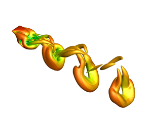
Hostname: page-component-745bb68f8f-hvd4g Total loading time: 0 Render date: 2025-01-28T04:11:58.896Z Has data issue: false hasContentIssue false

Dynamics of weighted flexible ribbons in a uniform flow

Published online by Cambridge University Press:  14 August 2024

Kui Liu
Affiliation:
Department of Modern Mechanics, University of Science and Technology of China, Hefei, Anhui 230026, PR China
Haibo Huang*
Affiliation:
Department of Modern Mechanics, University of Science and Technology of China, Hefei, Anhui 230026, PR China
*
Email address for correspondence: huanghb@ustc.edu.cn

Abstract

This study explores the dynamics of flexible ribbons with an added weight $G$ at the tail in uniform flow, considering key parameters like inflow Reynolds number ($Re_u$), mass ratio ($M_t$) and aspect ratio (${A{\kern-4pt}R}$). For two-dimensional ribbons, a simplified theoretical model accurately predicts equilibrium configurations and forces. Inspired by Barois & De Langre (J. Fluid Mech., vol. 735, 2013, R2), we introduce an important control parameter ($C_G$) that effectively collapses normalized forces and angle data. Vortex-induced vibration is observed, and Strouhal number ($St$) scaling laws with $C_G$ are identified. In three-dimensional scenarios, the model effectively predicts lift, but its accuracy in predicting drag is limited to situations with small $Re_u$ values. The flow along the side edges mitigates pressure differences, thereby suppressing vibration and uplift, particularly noticeable in the case of narrow ribbons. This study offers new insights into the dynamics of flexible bodies in uniform flow.

Type
JFM Papers
Copyright
© The Author(s), 2024. Published by Cambridge University Press

1. Introduction

The interaction between flexible structures and surrounding fluids is a common and well-known phenomenon in nature, as seen in the reconfiguration of plants (de Langre Reference de Langre2008), flapping of flags (Shelley & Zhang Reference Shelley and Zhang2011), swimming fish (Triantafyllou, Triantafyllou & Yue Reference Triantafyllou, Triantafyllou and Yue2000) and the flight of birds/insects (Wu Reference Wu2011). Studying the dynamics of these fluid–flexible structure systems is valuable for biologists seeking a deeper understanding of plant biology and the locomotion of aquatic and aerial animals (Nepf Reference Nepf2012; Lauder Reference Lauder2015). Moreover, the fundamental mechanisms uncovered can serve as inspiration for engineers designing high-performance biomimetic aerial/underwater vehicles or robots (Platzer et al. Reference Platzer, Jones, Young and Lai2008; Smits Reference Smits2019). The applications extend to energy extraction (Allen & Smits Reference Allen and Smits2001; Wu Reference Wu2011; Mathai et al. Reference Mathai, Tzezana, Das and Breuer2022), the paper industry (Watanabe et al. Reference Watanabe, Suzuki, Sugihara and Sueoka2002) and flow control (Shen et al. Reference Shen, Zhang, Yue and Triantafyllou2003; Sunil, Kumar & Poddar Reference Sunil, Kumar and Poddar2022). As a result, these issues have captivated human interest for several decades.

Previous studies, such as Alben, Shelley & Zhang (Reference Alben, Shelley and Zhang2002), Gao et al. (Reference Gao, Pan, Wang and Tian2020) and Sun et al. (Reference Sun, Peng, Yang, Xiong, Wang and Wang2022), have focused on drag reduction in fluid–flexible structure interactions. Classic theory for rigid bluff bodies suggests that drag ($F_d$) is proportional to the square of the oncoming flow speed ($U$), i.e. $F_d \sim U^2$ (Batchelor Reference Batchelor1967). However, flexible bodies under fluid loading undergo reconfiguration, decreasing the projected area perpendicular to the flow and adopting a more streamlined posture (Alben et al. Reference Alben, Shelley and Zhang2002; Buchak, Eloy & Reis Reference Buchak, Eloy and Reis2010; Luhar & Nepf Reference Luhar and Nepf2011; Schouveiler & Eloy Reference Schouveiler and Eloy2013). This reconfiguration results in a slower-growing form of drag, expressed as $F_d \sim U^{2 + \mathscr {V}}$, where $\mathscr {V}$ is the Vogel exponent (Vogel Reference Vogel1984Reference Vogel1989). Examples like tree leaves (Vogel Reference Vogel1989) or circular plastic sheets (Schouveiler & Boudaoud Reference Schouveiler and Boudaoud2006) demonstrate a much slower drag growth than the $U^2$ law as they roll into tighter cones in the fluid. In a two-dimensional (2-D) flowing soap film, a flexible fibre tethered at the midpoint exhibits drag scaling as $U^{4/3}$ (i.e. $\mathscr {V}=-2/3$) at high Reynolds numbers ($Re$), as observed in the experimental and theoretical study by Alben et al. (Reference Alben, Shelley and Zhang2002) and Alben, Shelley & Zhang (Reference Alben, Shelley and Zhang2004). Additionally, Zhu (Reference Zhu2008) numerically studied a compliant fibre tethered in a viscous flow at moderate $Re$ (i.e. $Re \in [10, 800]$) and found that the power law exponents decrease monotonically from approximately 2 towards 4/3 as $Re$ increases. Experimental investigations by Barois & de Langre (Reference Barois and de Langre2013) on the reconfiguration of flexible ribbons with added weight at the free end revealed that drag is nearly independent of free-stream velocity at high $Re$. This unique phenomenon is a focal point of the present study. In nature, plants laden with fruits naturally droop and sway in the wind. Similarly, in everyday scenarios, heavy objects are often added to the trailing edge of flags to prevent violent flapping. These observations highlight the relevance of weighted flexible structures in both natural and engineered systems.

However, the aforementioned studies do not address the flapping or vibration of bodies. When flow passes a bluff body, vortex shedding typically occurs with significant flow separation at relatively high $Re$. In such cases, a vortex wake, such as the Kármán vortex street, becomes observable. The periodic shedding of vortices results in oscillatory forces acting on the body, causing drag and lift in the streamwise and transverse directions, respectively. If the body is elastically mounted, it may undergo substantial vibration, termed vortex-induced vibration (VIV) (Williamson & Govardhan Reference Williamson and Govardhan2004). There is an extensive body of literature on VIV of rigid objects, including works by Sarpkaya (Reference Sarpkaya2004), Wu, Ge & Hong (Reference Wu, Ge and Hong2012), Raissi et al. (Reference Raissi, Wang, Triantafyllou and Karniadakis2019), Carlson, Currier & Modarres-Sadeghi (Reference Carlson, Currier and Modarres-Sadeghi2021) and Han et al. (Reference Han, de Langre, Thompson, Hourigan and Zhao2023), for interested readers to explore.

In the presence of an oncoming flow, flexible structures like flags, fibres or filaments may exhibit passive flapping motions (Zhang et al. Reference Zhang, Childress, Libchaber and Shelley2000; Jia et al. Reference Jia, Li, Yin and Yin2007; Jia & Yin Reference Jia and Yin2008; Kim et al. Reference Kim, Cossé, Huertas Cerdeira and Gharib2013). Taneda (Reference Taneda1968) experimentally explored various flags and observed that flags remain motionless in slow flows, transitioning to regular and irregular flapping states as the flow speed increases. The motion of flexible filaments in a flowing soap film was investigated by Zhang et al. (Reference Zhang, Childress, Libchaber and Shelley2000), revealing two distinct dynamical states for a single filament: stretched–straight and coherent flapping states. Shelley, Vandenberghe & Zhang (Reference Shelley, Vandenberghe and Zhang2005) studied oscillations of heavy flags through experiments and theoretical analysis, identifying a critical flow velocity triggering flag flapping. The corresponding Strouhal number ($St$) is consistent with that of swimming/flying animals for efficient cruising (Taylor, Nudds & Thomas Reference Taylor, Nudds and Thomas2003). Eloy et al. (Reference Eloy, Lagrange, Souilliez and Schouveiler2008) conducted experiments on the flutter of flexible plates with varying aspect ratios, highlighting the significance of three-dimensional (3-D) effects. Numerous numerical studies complement these experiments. For instance, 2-D simulations of a flag in viscous flow by Zhu & Peskin (Reference Zhu and Peskin2002) and Connell & Yue (Reference Connell and Yue2007), or inviscid flow by Alben & Shelley (Reference Alben and Shelley2008) confirmed bistable properties or hysteresis observed in experiments by Zhang et al. (Reference Zhang, Childress, Libchaber and Shelley2000) and Shelley et al. (Reference Shelley, Vandenberghe and Zhang2005). Connell & Yue (Reference Connell and Yue2007), by altering the mass ratio of 2-D flags and fluid, identified three distinct regimes: fixed-point, regular flapping and chaotic flapping regimes. The flapping of 3-D flags was simulated by Kim & Peskin (Reference Kim and Peskin2007) and Huang & Sung (Reference Huang and Sung2010), considering the effects of gravity. Additional numerical simulations of flexible flags or filaments can be found in works by Zhu & Peskin (Reference Zhu and Peskin2003), Zhu (Reference Zhu2009), Uddin, Huang & Sung (Reference Uddin, Huang and Sung2013), O'Connor & Revell (Reference O'Connor and Revell2019) and others.

In this study, we numerically investigate the dynamics of flexible ribbons in a uniform flow, with a weight $G$ added at the trailing edges. Notably, the only existing experimental research on this specific fluid–flexible structure problem was conducted by Barois & de Langre (Reference Barois and de Langre2013). However, their study lacked comprehensive discussion, omitting crucial details such as flow fields, potentially due to experimental measurement challenges. Additionally, they did not account for the effects of aspect ratio (${A{\kern-4pt}R}$) and the 2-D cases, which could yield notably different results, particularly when vibrations occur with a large aspect ratio. Furthermore, their study neglected viscous effects given the sufficiently large $Re$. To address these limitations, we conduct both 2-D and 3-D simulations at low Reynolds numbers (${\sim }O(10^2)$). Our investigation involves a thorough examination of ribbon reconfiguration and forces, and we establish a simplified theoretical model based on force decomposition for accurate predictions. Force decomposition allows us to isolate tangential forces, enabling a closer examination of viscous effects. Special attention is given to ribbon vibrations and the derivation of scaling laws. Additionally, we explore 3-D effects by varying the aspect ratio, conducting a detailed analysis of both 2-D and 3-D flow fields.

Adding weight to the end of the flexible ribbon serves several purposes in our study. Firstly, it simulates gravity's effect on flexible structures encountered in real-world scenarios. Our goal is to understand how gravity influences their motion and deformation. Secondly, adding weight enables us to manipulate the system's dynamic behaviour. Adjusting the centre of mass affects dynamic characteristics like vibration frequency, amplitude and mode shape of the ribbon. This provides more control variables and experimental parameters, enhancing our understanding of fluid–structure interaction. Furthermore, this approach offers insights and strategies for designing and optimizing flexible structures. Optimizing weight distribution improves performance across aerospace and mechanical engineering. For example, in flexible unmanned aerial vehicles, added weights may enhance flight dynamics.

Note that both 2-D and 3-D simulations are essential in our study. Considering that achieving a much wider range of ${A{\kern-4pt}R}$ would demand significant computational resources, we selected a feasible range that still allowed us to investigate relevant 3-D effects. The 2-D simulations are valuable as they correspond to cases where ${A{\kern-4pt}R}$ approaches infinity, assuming deformation in the spanwise direction can be neglected. This simplification enables us to focus on the fundamental behaviour of the ribbon and its interaction with the surrounding fluid. Besides, conducting 2-D simulations aligns with our theoretical analysis, which is inherently two-dimensional. This allows for a direct comparison between theoretical predictions and numerical simulations, facilitating a deeper understanding of the fluid–structure interaction phenomenon.

The remainder of this paper is organized as follows. In § 2, we present the physical problem and mathematical formulation. The numerical method and validation are detailed in § 3. In § 4, we discuss comprehensive results, and concluding remarks are provided in § 5.

2. Physical problem and mathematical formulation

The schematic diagrams of the 2-D and 3-D flexible ribbons considered in our study are illustrated in figure 1. These flexible ribbons, characterized by a length $L$ (and width $W$ in 3-D cases), are immersed in a uniform flow with an oncoming speed $U$. The leading edge of the ribbon is stationary, while a weight $G$ is affixed at the trailing edge, inducing a natural droop. The remaining sections of the ribbon have the freedom to move and passively deform, facilitated by fluid–structure interactions.

Figure 1. Schematic diagrams illustrating 2-D (a) and 3-D (b) flexible ribbons in a uniform flow. Here, $U$ represents the oncoming flow speed, $L$ and $W$ denote the chord and span length of the ribbon, respectively, $G$ is the weight added at the trailing edge, $\theta _l$ is the angle between the tangent direction of the leading edge and the horizontal direction and $s$ as well as $(s_1, s_2)$ represent the curvilinear coordinates on the ribbons.

We employ the incompressible Navier–Stokes equations to model and solve the fluid flow,

(2.1)$$\begin{gather} \frac{\partial \boldsymbol{v}}{\partial t}+\boldsymbol{v} \boldsymbol{\cdot}\boldsymbol{\nabla} \boldsymbol{v}=-\frac{1}{\rho} \boldsymbol{\nabla} p+\frac{\mu}{\rho} \nabla^{2} \boldsymbol{v}+\boldsymbol{f}_{b}, \end{gather}$$
(2.2)$$\begin{gather}\boldsymbol{\nabla} \boldsymbol{\cdot}\boldsymbol{v}=0, \end{gather}$$

where $\boldsymbol {v}$ is the velocity, $p$ is the pressure, $\rho$ is the density of the fluid, $\mu$ is the dynamic viscosity and $\boldsymbol {f}_{b}$ denotes the Eulerian momentum force acting on the surrounding fluid due to the immersed boundary.

To characterize the deformation and motion of the ribbon within a Lagrangian coordinate system, we employ the structural equation. In the case of 3-D scenarios, the structural equation is formulated as follows (Huang & Sung Reference Huang and Sung2010; Hua, Zhu & Lu Reference Hua, Zhu and Lu2014):

(2.3)\begin{align} \rho_s h \frac{\partial^2 \boldsymbol{X}}{\partial t^2}=\sum_{i, j=1}^2 \frac{\partial}{\partial s_i}\left\{\varphi_{i j} \left[\delta_{i j}-\left(\frac{\partial \boldsymbol{X}}{\partial s_i} \boldsymbol{\cdot} \frac{\partial \boldsymbol{X}}{\partial s_j}\right)^{-1 / 2}\right] \frac{\partial \boldsymbol{X}}{\partial s_j}-\frac{\partial}{\partial s_j} \left(\gamma_{i j} \frac{\partial^2 \boldsymbol{X}}{\partial s_i \partial s_j}\right)\right\}+ \boldsymbol{F}_s + \boldsymbol{F}_{g}, \end{align}

where $\boldsymbol {X}(s_1, s_2, t)=(X(s_1, s_2, t), Y(s_1, s_2, t), Z(s_1, s_2, t))$ is the position vector of the ribbon, $s_1$ and $s_2$ are the chordwise and spanwise Lagrangian coordinates, respectively, $\rho _{s}$ is the structural mass density, $h$ is the structural thickness, $\boldsymbol {F}_{s}$ is the Lagrangian force exerted on the plate by the surrounding fluid, $\boldsymbol {F}_{g} = G \boldsymbol g / g$ is the weight added at the trailing edge (here, $g$ is the magnitude of gravitational acceleration $\boldsymbol g$) and $\delta _{i j}$ is the Kronecker delta function. Matrix $\varphi _{i j}$ is the in-plane effect matrix, where $\varphi _{11}=\varphi _{22}=E h$ is the structural stretching stiffness and $\varphi _{12}$ is the structural shearing stiffness. Matrix $\gamma _{ij}$ represents the out-of-plane effect matrix associated with bending and twisting stiffness, where $\gamma _{11} = EI$ denotes the chordwise bending stiffness. At the leading edge ($s_1 = 0$), the simply supported condition is adopted, i.e.

(2.4a,b)\begin{equation} \boldsymbol{X}=(0, 0, s_2),\quad \frac{\partial^2 \boldsymbol{X}}{\partial s_1^2}=0. \end{equation}

At the trailing edge ($s_1 = L$) and two other free edges ($s_2 = 0$ or $W$), the boundary conditions are

(2.5a,b)\begin{equation} \varphi_{i j}\left[\delta_{i j}-\left(\frac{\partial \boldsymbol{X}}{\partial s_i} \boldsymbol{\cdot} \frac{\partial \boldsymbol{X}}{\partial s_j}\right)^{-1 / 2}\right] \frac{\partial \boldsymbol X}{\partial s_j}-\frac{\partial}{\partial s_j}\left(\gamma_{i j} \frac{\partial^2 \boldsymbol X}{\partial s_i \partial s_j}\right)=0,\quad \frac{\partial^2 \boldsymbol{X}}{\partial s_i \partial s_j}=0. \end{equation}

Here, the Einstein summation convention is not applied on $i$ and $j$ ($i, j=1, 2$). In addition, the weight $G=W m_t g$ is evenly distributed at the trailing edge (see figure 1b), where $m_t$ is the mass per unit length of the additional weight.

For the 2-D cases, the structural equation (2.3) degenerates into the following form (Zhu & Peskin Reference Zhu and Peskin2002; Connell & Yue Reference Connell and Yue2007; Hua, Zhu & Lu Reference Hua, Zhu and Lu2013):

(2.6)\begin{equation} \rho_{s} h \frac{\partial^{2} \boldsymbol{X}}{\partial t^{2}}-\frac{\partial}{\partial s} \left[E h\left(1-\left|\frac{\partial \boldsymbol{X}} {\partial s}\right|^{-1}\right) \frac{\partial \boldsymbol{X}}{\partial s}\right]+E I \frac{\partial^{4} \boldsymbol{X}}{\partial s^{4}}=\boldsymbol{F}_{s} + \boldsymbol{F}_{g}, \end{equation}

where $s$ is the Lagrangian coordinate, $\boldsymbol {X}(s, t)=(X(s, t), Y(s, t))$ is the position vector of the ribbon. At the leading edge of the ribbon ($s=0$), the simply supported condition (2.4a,b) becomes

(2.7a,b)\begin{equation} \boldsymbol{X}=\left(0, 0\right),\quad \frac{\partial^2 \boldsymbol{X}}{\partial s^2}=0. \end{equation}

At the free end ($s=L$), the boundary conditions are

(2.8a,b)\begin{equation} -E h\left(1-\left|\frac{\partial \boldsymbol{X}}{\partial s}\right|^{-1}\right) \frac{\partial \boldsymbol{X}}{\partial s} + E I \frac{\partial^3 \boldsymbol{X}}{\partial s^3}=0,\quad \frac{\partial^2 \boldsymbol{X}}{\partial s^2}=0. \end{equation}

Besides, the weight $G=1 \cdot m_t g$ (considering unit depth) is concentrated at the trailing edge (see figure 1a).

In our study, the fluid density $\rho$, the dynamic viscosity $\mu$ and the dimensional length of the ribbon $L$ are fixed. To normalize the above equations, the characteristic quantities $\rho$, $L$ and $U_{ref} = \kappa \mu / \rho L$ are chosen, where $\kappa =200$ is a constant (note that other values of $\kappa$ are also acceptable, and would not alter the trends and findings presented in our study). Therefore, the characteristic time is $T = L / U_{ref}$, and the gravitational acceleration is $g = U_{ref}^2 / L$. Based on dimensional analysis, the following dimensionless governing parameters are introduced: the aspect ratio ${A{\kern-4pt}R} = W/L$, the Reynolds number based on the oncoming flow speed $Re_u=\rho U L / \mu$, the mass ratio of the ribbon to the fluid $M=\rho _{s} h/ \rho L$, the mass ratio of additional weight at the trailing edge to the fluid $M_t=m_t / \rho L^2$, the stretching stiffness $S =E h / \rho U_{ref}^{2} L$ and the bending stiffness $K =E I / \rho U_{ref}^{2} L^{3}$.

3. Numerical method and validation

The lattice Boltzmann method (Chen & Doolen Reference Chen and Doolen1998) is employed for the numerical solution of the Navier–Stokes equations, while a finite element method is utilized to model the motion of the flexible plate (Doyle Reference Doyle2001). The immersed boundary method (Zhu & Peskin Reference Zhu and Peskin2002) is employed to couple the fluid and structure solvers. To enforce the no-slip boundary condition, the body force term $\boldsymbol {f}_{b}$ in (2.1) acts as an interaction force between the fluid and the immersed boundary. The deformation of the plate is addressed using the corotational scheme (Doyle Reference Doyle2001), which is adept at handling large displacements. Further details on the numerical methods can be found in our previous papers (Hua et al. Reference Hua, Zhu and Lu2013; Huang, Wei & Lu Reference Huang, Wei and Lu2018; Zhang, Huang & Lu Reference Zhang, Huang and Lu2020).

The simulations are performed on a computational domain in the range $[-15, 25] \times [-15, 15]$ in the $x$ and $y$ directions for 2-D cases, and $[-10, 30] \times [-10, 10] \times [-10, 10]$ in the $x$, $y$ and $z$ directions for 3-D cases. This domain size is sufficiently large to eliminate any boundary effects. Initially, the fluid's velocity field is $U \boldsymbol e_x$ throughout the domain, where $\boldsymbol e_x$ is the unit vector in the $x$ direction. A uniform velocity $U \boldsymbol e_x$ is imposed at the upstream boundary and the side boundaries of the fluid computational domain. At the downstream boundary, a convective boundary condition $\partial \boldsymbol {v} / \partial t + U \partial \boldsymbol {v} / \partial x = \boldsymbol {0}$ is specified.

To validate the numerical method, simulations of 2-D and 3-D flags in a uniform flow are conducted. In the 2-D case, the non-dimensional parameters are $Re=200$, $K=0.0015$, $M=1.5$, $S=1000$ and Froude number $Fr=g L / U^2=0.5$ (Huang et al. Reference Huang, Shin and Sung2007). For the 3-D case, the parameters are $Re=200$, $K=0.0001$, $M=1.0$, $S=1000$, $Fr=0$ and ${A{\kern-4pt}R} =1$ (Huang & Sung Reference Huang and Sung2010). The results are depicted in figure 2, showing good agreement with results in the literature (Huang et al. Reference Huang, Shin and Sung2007; Huang & Sung Reference Huang and Sung2010).

Figure 2. Validations for cases: (a) transverse displacement of the trailing edge of the 2-D flag with $Re=200$, $K=0.0015$, $M=1.5$, $S=1000$ and $Fr=0.5$ (Huang, Shin & Sung Reference Huang, Shin and Sung2007); (b) transverse displacement of the centre of the trailing edge of the 3-D flag with $Re=200$, $K=0.0001$, $M=1.0$, $S=1000$, $Fr=0$ and ${A{\kern-4pt}R} =1$ (Huang & Sung Reference Huang and Sung2010).

Besides, we have also made a direct comparison of our results with those of Barois & de Langre (Reference Barois and de Langre2013), as shown in figure 3. In this comparison, the $G$-normalized drag $F_d / G$ of the 3-D ribbon is presented as a function of $C_G$ with $M_t = 1$ and ${A{\kern-4pt}R} = 0.5$, where the definition of $C_G$ in 3-D scenarios is $C_G = {\rho U^2 L W}/{2G}$. Despite our $Re_u$ being approximately one or two orders of magnitude smaller than theirs (${\sim }O(10^2\unicode{x2013}10^3)$ compared with ${\sim }O(10^3\unicode{x2013}10^5)$), our results capture the variation trend of the $F_d/G$ curve well. Especially when $C_G<1$, our results are consistent with their experimental findings. This indicates the significance of our study within the $Re_u \sim O(10^2\unicode{x2013}10^3)$ range. However, for $C_G>1$, we observe that our $F_d/G$ values are notably larger than their corresponding values. This discrepancy may be due to the significant skin friction caused by viscous effects in our study, owing to our lower $Re_u$, as discussed in § 4.2.1.

Figure 3. The $G$-normalized drag $F_d / G$ of the 3-D ribbon as a function of $C_G$ with $M_t = 1$ and ${A{\kern-4pt}R} = 0.5$. The experimental results of Barois & de Langre (Reference Barois and de Langre2013) are also presented with ${A{\kern-4pt}R} \approx 0.1$.

Furthermore, our numerical strategy has been successfully validated and applied to study various flow problems, including tandem flexible inverted flags in a uniform flow (Huang et al. Reference Huang, Wei and Lu2018), the impact of trailing-edge shape on the self-propulsive performance of heaving flexible plates (Zhang et al. Reference Zhang, Huang and Lu2020) and the scaling laws of the self-propulsive performance of flexible plates (Liu, Liu & Huang Reference Liu, Liu and Huang2022). Additional detailed numerical validations are available in these referenced papers.

The outcomes of the grid independence and time-step independence assessments for the 2-D and 3-D flexible ribbons are depicted in figure 4. It indicates that $\Delta x / L=0.01$ and $\Delta t / T=0.00025$ are suitable for the 2-D cases, while $\Delta x / L=0.025$ and $\Delta t / T=0.000625$ are sufficient for the 3-D cases to attain accurate results. Consequently, we adopt these mesh sizes and time-step sizes in our subsequent simulations.

Figure 4. Grid independence and time-step independence study for (a) the 2-D ribbon with $M_t = 1$ and $Re_u = 200$ and (b) the 3-D ribbon with $M_t = 1$, $Re_u = 200$ and ${A{\kern-4pt}R} =0.25$. The streamwise force $F_x$ normalized by $F_{ref} = (1/2) \rho U_{ref}^2 L$ as a function of time is presented.

4. Results and discussion

In the present simulations, certain parameters are held constant: mass ratio of the ribbon to the fluid ($M = 0.5$), bending stiffness ($K = 10^{-4}$) and stretching stiffness ($S=10^4$). The choice of a large $S$ ensures that the ribbon is nearly inextensible, while a small $K$ ensures that the ribbon is fully compliant with the surrounding flow, aligning with the experimental findings of Barois & de Langre (Reference Barois and de Langre2013). The selected value for $M$ also conforms to previous studies on flexible bodies in a uniform flow (Huang & Sung Reference Huang and Sung2010; Hua et al. Reference Hua, Zhu and Lu2014; Sun et al. Reference Sun, Peng, Yang, Xiong, Wang and Wang2022), where $M$ ranges from $10^{-1}$ to $10^0$. The remaining key parameters, namely the inflow Reynolds number $Re_u$, the mass ratio of the additional weight at the trailing edge $M_t$ and the aspect ratio ${A{\kern-4pt}R}$, are left variable. Both 2-D and 3-D cases are considered, and the corresponding results are presented in §§ 4.1 and 4.2, respectively.

4.1. Analysis of two-dimensional results

In the 2-D scenarios, the aspect ratio ${A{\kern-4pt}R} = \infty$, and we investigate the effects of $Re_u$ ($\in [50,800]$ with an interval of 50) and $M_t$ ($=1, 2$ and $3$). In Appendix A, we demonstrate that the initial angle of the ribbon has no impact on the statistics of interest, such as time-averaged forces. Once released from the initial state, the system promptly reaches an equilibrium state, where the ribbon may undergo periodic oscillations.

Our initial focus is on quasi-static results (§ 4.1.1) to propose a simplified model (§ 4.1.2). In this context, quantitative results are presented as time-averaged values unless explicitly specified otherwise. For instance, the time-averaged drag and lift are defined as $F_d = f_1 \int _{t^{\prime }}^{t^{\prime }+1/f_1} F_x(t) \,\mathrm {d} t$ and $F_l = f_1 \int _{t^{\prime }}^{t^{\prime }+1/f_1} F_y(t) \,\mathrm {d} t$, respectively, where $f_1$ represents the dominant frequency or flapping frequency, and $F_x(t)$ and $F_y(t)$ denote the instantaneous streamwise and transverse forces of the ribbon. The analysis of kinematic characteristics (i.e. vibrations) and flow fields of the system will be conducted in § 4.1.4.

4.1.1. Reconfiguration and forces

The discussion on the reconfiguration of the ribbons is presented first, as depicted in figure 5. In slow flows (i.e. small $Re_u$), the ribbon sags downwards due to gravity acting on the trailing edge. As $Re_u$ increases, the ribbon gradually lifts upwards with noticeable bending deformations (figure 5), presenting a more streamlined shape. The projection length of the ribbon in the $x$ and $y$ directions, denoted as $L_x$ and $L_y$ respectively, monotonically increases and decreases with the flow speed, as illustrated in figure 6. These observations align with the fundamental characteristics of flexible body reconfiguration in flow (Alben et al. Reference Alben, Shelley and Zhang2002; Gosselin, de Langre & Machado-Almeida Reference Gosselin, de Langre and Machado-Almeida2010).

Figure 5. The equilibrium configurations of the ribbons for (a) $M_t = 1$, $Re_u = 100\unicode{x2013}400$, (b) $M_t = 2$, $Re_u = 100\unicode{x2013}600$ and (c) $M_t = 3$, $Re_u = 100\unicode{x2013}700$. Here, the curves represent time-averaged configurations, as the ribbons undergo periodic oscillation in 2-D scenarios. In each panel, the $Re_u$ values of the cases increase gradually from left to right, with an interval of 100.

Figure 6. The normalized projected length of the ribbon in the $x$ and $y$ directions, i.e. (a) $L_x$ and (b) $L_y$.

It is noteworthy that higher speeds can induce self-collision of the ribbon due to violent vibrations (see § 4.1.4). This leads to simulation failure, and the corresponding cases are discarded. Thus, there exists a critical value of $Re_u$, denoted as $Re_u^c$, beyond which the system becomes unstable. The value of $Re_u^c$ is dependent on the mass ratio of the weight added at the trailing edge $M_t$. We observed that, for $M_t = 1$, 2 and 3, the critical Reynolds number $Re_u^c$ is approximately 450, 600 and 750, respectively. Consequently, in figures 6 and 7, only cases with $Re_u \leq Re_u^c$ are plotted. This observation of $Re_u^c$ increasing with $M_t$ agrees with expectations, as a larger $M_t$ typically enhances system stability.

Figure 7. The normalized time-averaged (a) leading-edge inclination angle $\theta _l$, (b) drag $F_d$, (c) lift $F_l$ and (d) leading-edge tension $T_l$ of the 2-D ribbons as functions of $Re_u$ for various $M_t$. The hollow circles mark the positions where $\theta _l = 0$.

In addition to $L_x$ and $L_y$, the leading-edge inclination angle $\theta _l$ can also be employed to quantitatively describe the ribbon's reconfiguration (see figure 1a). Figure 7(a) illustrates $\theta _l$ as a function of $Re_u$. It is noted that $\theta _l$ exhibits an initial increase followed by a slight decrease with the increase of $Re_u$. The decrease in $\theta _l$ for large $Re_u$ is associated with the increase in the streamwise projection length $L_x$ of the ribbon (see figures 5 and 6(a), and note that the ribbon's total length remains constant due to its inextensibility). Its further mechanism will be discussed in figure 8. It is noteworthy that $\theta _l$ can significantly exceed 0, as evident in figure 7(a), where the maximum value of $\theta _l$ is approximately $36^\circ$, or in figure 5, where the ribbon conspicuously protrudes upwards for large $Re_u$. This result diverges from the experiments conducted by Barois & de Langre (Reference Barois and de Langre2013), where the maximum value of $\theta _l$ is 0. A more in-depth analysis of this disparity is provided in the subsequent sections.

Figure 8. Time-averaged pressure contours around the ribbon for $Re_u = 350$ (a), 400 (b) and 450 (c) with $M_t = 1$. Solid and dashed lines denote the positive and negative normalized pressure contours, respectively.

The flow-induced reconfiguration significantly influences the forces acting on the ribbons (Schouveiler & Boudaoud Reference Schouveiler and Boudaoud2006; Luhar & Nepf Reference Luhar and Nepf2011). Figure 7(bd) presents the time-averaged drag $F_d$, lift $F_l$ and leading-edge tension $T_l$ of the ribbon as functions of $Re_u$ for different $M_t$. It is observed that, at small $Re_u$, the drag of the ribbon adheres well to the classical quadratic law, i.e. $F_d \sim Re_u^2 \sim U^2$ (see the dashed line in figure 7b). This behaviour is attributed to the minimal deformation of the ribbon at small $Re_u$. For instance, at $Re_u \leq 250$ with $M_t = 3$, the ribbon exhibits $L_y \geq 0.92$ (see figure 6b), resembling an upright rigid plate. Consequently, the drag of the ribbon at small $Re_u$ mimics that of rigid bluff bodies. The $U^2$ growth in drag also implies the predominance of form drag while skin friction can be neglected (Alben et al. Reference Alben, Shelley and Zhang2002). In the absence of skin friction, the tension of the ribbon is uniform and equivalent to the weight $G$ added at the trailing edge (see § 4.1.2). Therefore, at small $Re_u$, the leading-edge tension $T_l$ of the ribbon remains nearly constant (see figure 7d), i.e. $T_l \approx G$ (note that the value of normalized weight $G/F_{ref}$ is twice that of $M_t$ due to the factor $1/2$ in $F_{ref} = (1/2) \rho U_{ref}^2 L$).

As $Re_u$ increases, the influence of skin friction becomes significant. The hollow circles in figure 7 mark the positions where $\theta _l = 0$, signifying a point where skin friction starts to play a crucial role. Figure 7(d) indicates that, when $\theta _l > 0$, the leading-edge tension $T_l$ experiences a substantial increase with the rising $Re_u$. This phenomenon may be attributed to the fact that, under large $Re_u$ conditions ($\theta _l > 0$), the ribbon's shape tends to align more parallel to the oncoming flow (see figure 5), facilitating the generation of skin friction. Consequently, skin friction contributes to the tension in the ribbon, resulting in $T_l > G$ for high $Re_u$ (figure 7d).

Here, we would like to estimate the magnitude of the skin friction to better elucidate whether it plays an important role. The skin friction can be approximated as viscous drag per unit width on a flat plate aligned with the flow, expressed as: $F_{vis} = 1.33\rho U^2 L_x Re_u^{-1/2}$ (Batchelor Reference Batchelor1967; Alben et al. Reference Alben, Shelley and Zhang2002) (i.e. the $U^{3/2}$ scaling), where $L_x$ is the length of the plate (in our study, it is the projected length of the ribbon in the $x$ direction). The dimensionless skin friction is given by: $\hat F_{vis} = F_{vis} / F_{ref}=1.33\rho U^2 L_x Re_u^{-1/2} / (0.5 \rho U_{ref}^2 L ) = 2.66 Re_u^{3/2} L_x / ( \kappa ^2 L )$. Through calculation, when $Re_u$ is small, $F_{vis}$ is at least one order of magnitude smaller than the total drag $F_d$, indicating its negligible contribution (i.e. $F_{vis} / F_d < 10^{-1}$). Specifically, for the case with $Re_u = 400$ and $M_t = 2$, $F_{vis} / F_d \approx 0.09$, thus the skin friction can be ignored. However, at large $Re_u$, $F_{vis}$ significantly increases. For instance, for $Re_u = 600$ and $M_t = 2$, $F_{vis} / F_d \approx 0.17$, which closely matches the percentage increase of $T_l$ compared with $G$ in figure 7(d). Alternatively, the approximate 17 % increase can be directly observed from figure 12(a). This indicates that, at large $Re_u$, the skin friction may have a significant effect on leading-edge tension increment. These conclusions are consistent with what we have found and summarized in the above analysis and § 4.1.2.

Remarkably, it is observed that, when $\theta _l > 0$, the change in $F_d$ remains small, and $F_d$ approximates $G$ as $Re_u$ increases (see figure 7b). In other words, the drag appears to be independent of the oncoming flow speed, resembling the findings of Barois & de Langre (Reference Barois and de Langre2013). In the experiments by Barois & de Langre (Reference Barois and de Langre2013), skin friction was neglected as $Re_u \sim O(10^4)$. Consequently, the tension in the ribbon equalled the weight added at the trailing edge, i.e. $T_l = G$. As $Re_u$ increased, they observed that the leading edge of the ribbon remained horizontal (Barois & de Langre Reference Barois and de Langre2013), implying $\theta _l = 0$. Therefore, the drag remained constant since $F_d = T_l \cos \theta _l = G$ (see figure 25a). In contrast, in our study, $\theta _l$ continues to increase after reaching 0 (figure 7a), resulting in a further reduction in the transverse projection length $L_y$ (figure 6b) and the form drag. However, the increased skin friction, as detailed in the next section, compensates for the reduced form drag, thereby maintaining the total drag substantially unchanged (figure 7b).

Concerning the lift $F_l$, it primarily relies on the transverse pressure difference across the ribbon. Notably, a larger transverse pressure difference results in a greater $\theta _l$. Consequently, $F_l$ exhibits a similar trend to $\theta _l$ as $Re_u$ increases (see figure 7c). In figure 8, we present time-averaged pressure contours around the ribbon for $Re_u = 350$, 400 and 450 with $M_t = 1$. It is seen that, with the rise in $Re_u$, the high-pressure region beneath the ribbon diminishes and shifts towards the trailing edge, indicating a decrease in the pressure difference across the ribbon. Hence, beyond certain thresholds (e.g. $Re_u = 350$ for $M_t = 1$ and $Re_u = 450$ for $M_t = 2$), both $F_l$ and $\theta _l$ decline as $Re_u$ increases, as depicted in figure 7(a,c). Additionally, since $F_l = T_l \sin \theta _l + G$ (see figure 25a), it becomes evident that $F_l \approx G$ when $\theta _l = 0$ (indicated by the hollow circles in figure 7c).

Furthermore, it is observable that an increase in $M_t$ (or the weight $G$) leads to an approximately proportional increase in $T_l$ (figure 7d). This, in turn, results in a proportional increase in $F_d$ and $F_l$ when $Re_u$ is large (figure 7b,c). Therefore, $G$ emerges as a pivotal characteristic force of the system, offering insights for force rescaling in § 4.1.3.

4.1.2. Simplified theoretical model

To facilitate a more insightful analysis of the fluid–flexible structure problem, it is necessary to establish a simplified theoretical model. In Appendix B, we achieve this by decomposing the force acting on the ribbon. Next, we would like to check whether the model can effectively predict the equilibrium configurations and forces of the ribbons.

According to (B7), we can obtain the local inclination angle $\theta$ at different positions of the ribbon. Specifically, in (B7), let $\hat s = 0$ (i.e. the leading edge), we can get that

(4.1)\begin{equation} \theta_l = \theta(0) =-\frac{\rm \pi}{2}+\frac{f_n L}{G}, \end{equation}

or

(4.2)\begin{equation} \frac{f_n L}{G} = \theta_l + \frac{\rm \pi}{2}. \end{equation}

Substituting (4.2) into (B7), we have

(4.3)\begin{equation} \theta(\hat{s})=\theta_l-\hat{s}\left(\theta_l+\frac{\rm \pi}{2}\right). \end{equation}

The equations (4.3) and (B7) describe the theoretical equilibrium shape of the ribbon. In practical terms, (4.3) is more useful than (B7) because it is more convenient to observe $\theta _l$ rather than $f_n$ in experiments. Figure 9 shows the local inclination angle $\theta$ along the ribbon for various $Re_u$ with $M_t = 2$, where symbols and lines represent numerical and theoretical (according to (4.3)) results, respectively. It is seen that the theoretical model effectively predicts $\theta$ along the ribbon when $Re_u$ is not too large. However, the model fails for large $Re_u$, primarily because, under those circumstances, the large tangential force stretches the ribbon in the streamwise direction, and the shape is no longer a circular arc (see the cases with large $Re_u$ in figure 5).

Figure 9. The local inclination angle $\theta$ along the ribbon for various $Re_u$ with $M_t = 2$. Symbols and lines represent numerical and theoretical (according to (4.3)) results, respectively.

This theoretical model is also applicable for predicting the drag and lift of the ribbon. Although (4.2) has provided the relationship between $f_n$ and $\theta _l$, we aim to validate the results through numerical simulations. Figure 10 illustrates the $G$-normalized total normal force $f_n L / G$ as a function of the leading-edge inclination angle $\theta _l$. It is observed that, for all $M_t$, $f_n L / G$ well satisfies the linear relationship with respect to $\theta _l$ with the slope $\gamma = 1.1$, while the slope given by (4.2) is 1. This slight difference may arise from the non-uniform distribution of $f_n$ near the edges (see figure 26a). The tangential force might also influence the slope as it alters the ribbon shape (i.e. $\theta _l$) and local tension magnitude. Considering these factors, $\gamma$ can be regarded as a correction parameter, and (4.2) can be modified to

(4.4)\begin{equation} f_n = \frac {\gamma G}{L} \left(\theta_l + \frac{\rm \pi}{2}\right),\quad (\gamma = 1.1). \end{equation}

According to (4.3) and (4.4), the total drag $F_d$ and lift $F_l$ of the ribbon can be calculated as follows:

(4.5)\begin{align} F_d = \int_0^1-f_n \sin \theta {\cdot} L \,\mathrm{d} \hat{s} &= \int_0^1-\frac{\gamma G}{L} \left(\theta_l+\frac{\rm \pi}{2}\right) \sin \left[\theta_l-\hat{s}\left(\theta_l+\frac{\rm \pi}{2}\right)\right] {\cdot} L \,\mathrm{d} \hat{s} \nonumber\\ &= \gamma G \cos \theta_l, \end{align}
(4.6)\begin{align} F_l=\int_0^1 f_n \cos \theta {\cdot} L \,\mathrm{d} \hat{s} &= \int_0^1 \frac{\gamma G}{L}\left(\theta_l+\frac{\rm \pi}{2}\right) \cos \left[\theta_l-\hat{s}\left(\theta_l+\frac{\rm \pi}{2}\right)\right] {\cdot} L \,\mathrm{d} \hat{s} \nonumber\\ &= \gamma G(1+\sin \theta_l). \end{align}

Figure 11 presents the $G$-normalized drag $F_d / G$ and lift $F_l / G$. The numerical results align well with the theoretical values given by (4.5) and (4.6). However, small discrepancies are noticed for cases with $\theta _l \approx 0.2{\rm \pi}$ (see figure 11a). This is not surprising as the assumptions made in the theoretical prediction, $f_n \approx C$ and $f_\tau \approx 0$, are broken in these large-$Re_u$ cases.

Figure 10. The $G$-normalized total normal force $f_n L / G$ as a function of the leading-edge inclination angle $\theta _l$ for different $M_t$. The dash-dotted line is the fitting curve: ${f_n L}/{G} = \gamma (\theta _l + {{\rm \pi} }/{2})$, with a slope of $\gamma = 1.1$ and $R^2 = 0.99$.

Figure 11. The $G$-normalized (a) drag $F_d / G$ and (b) lift $F_l / G$ as functions of $\theta _l$ for various $M_t$. The dash-dotted lines represent the theoretical predictions given by (4.5) and (4.6).

Next, we examine the contribution of normal and tangential forces to drag and lift (i.e. the $x$ and $y$ component forces experienced by the ribbon). Let us begin by investigating the contribution of normal and tangential forces to drag

(4.7a,b)\begin{equation} F_{n, x} = f_1 \int_{t^{\prime}}^{t^{\prime}+1/f_1} \int_0^L f_{n, x}(s,t) \,\mathrm{d} s \,\mathrm{d} t,\quad F_{\tau, x} = f_1 \int_{t^{\prime}}^{t^{\prime}+1/f_1} \int_0^L f_{\tau, x}(s,t) \,\mathrm{d} s \,\mathrm{d} t, \end{equation}

where $f_1$ is the vibration frequency of the ribbon (see § 4.1.4). The contribution of normal and tangential forces to lift

(4.8a,b)\begin{equation} F_{n, y} = f_1 \int_{t^{\prime}}^{t^{\prime}+1/f_1} \int_0^L f_{n, y}(s,t) \,\mathrm{d} s \,\mathrm{d} t,\quad F_{\tau, y} = f_1 \int_{t^{\prime}}^{t^{\prime}+1/f_1} \int_0^L f_{\tau, y}(s,t) \,\mathrm{d} s \,\mathrm{d} t. \end{equation}

In figure 12, we present these forces as functions of $Re_u$ for cases with $M_t = 2$. It is observed that, when $Re_u \leq 300$, the drag almost entirely comes from the normal force since $F_d \approx F_{n, x}$ and $F_{\tau, x} \approx 0$ (see figure 12a). When $Re_u > 300$, the tangential force begins to exert its effect in generating drag, contributing approximately 15 % of the drag for $Re_u = 600$ (see figure 12a). These results are consistent with our estimation of skin friction or tangential force in § 4.1.1. Therefore, for high $Re_u$ (or $\theta _l$), the drag calculated by the theoretical model (4.5) is smaller than the actual one (see figure 11a).

Figure 12. (a) The drag $F_d$, the total $x$-component of $\boldsymbol f_n$ and $\boldsymbol f_\tau$ (i.e. $F_{n, x}$ and $F_{\tau, x}$) and (b) the lift $F_l$, the total $y$-component of $\boldsymbol f_n$ and $\boldsymbol f_\tau$ (i.e. $F_{n, y}$ and $F_{\tau, y}$) as functions of $Re_u$ with $M_t = 2$. The forces are rescaled using $G$.

On the other hand, as shown in figure 12(b), the tangential force contributes less to the lift, and almost all the lift is generated by the normal force, i.e. $F_l \approx F_{n, y}$. Hence, the theoretical model works well for the lift, even when $Re_u$ (or $\theta _l$) is large (see figure 11b).

4.1.3. Normalization analysis and rescaling

In § 4.1.1, we presented key results of the ribbons vs $Re_u$, normalizing the forces by $F_{ref}= (1/2) \rho U_{ref}^2 L$. However, these data did not collapse (see figure 7). The introduction of new scaling parameters is necessary to achieve a possible uniform scaling and enhance our understanding of the underlying mechanisms of the problem.

Note that the forces involved in the system mainly include the fluid force characterized by $\rho U^2 L$, the elastic force characterized by $EI / L^2$ and the weight $G$ added at the trailing edge. Since the bending stiffness of the ribbon in our study is $K =E I / \rho U_{ref}^{2} L^{3} = 10^{-4}$, we can see that $E I / L^{2} = 10^{-4} \rho U_{ref}^{2} L \approx 10^{-4} \rho U^2 L$, i.e. the elastic force is negligible because it is much smaller than the fluid force. While $G$ and $\rho U^2 L$ are of the same order of magnitude. Therefore, the behaviour of the ribbon is primarily governed by the balance between $G$ and the characteristic fluid force $\rho U^2 L$. Hence, a key non-dimensional parameter can be defined as (Barois & de Langre Reference Barois and de Langre2013)

(4.9)\begin{equation} C_G = \frac{\rho U^2 L}{2G}, \end{equation}

which can also be regarded as the $G$-normalized characteristic fluid force. It is inspired by the theoretical model in § 4.1.2, where $f_n$, $F_d$ and $F_l$ are all proportional to $G$ (see (4.4), (4.5) and (4.6)). This suggests that $G$ serves as the characteristic force of the system, and all forces, including the characteristic fluid force $\rho U^2 L$, should be rescaled using $G$.

The forces and angle data in the new scaling are plotted in figure 13. Remarkably, this scaling collapses the data well for all $M_t$, compared with figure 7. Additionally, for small $C_G$, the $G$-normalized drag can be scaled as $F_d / G \sim C_G$, corresponding to the $U^2$ growth of drag in figure 7(b); while $F_d / G \approx 1$ when $C_G$ is large (see figure 13b), corresponding to $F_d \approx G$ (figure 7b). It is also noteworthy that, similar to $Re_u^c$, there is a critical $C_G$, i.e. $C_G^c$, beyond which the system is unstable due to self-collision of the ribbon. For various $M_t$, $C_G^c$ remains almost constant, at approximately $2.4$ (see figure 13). This consistency suggests that $C_G^c$ effectively characterizes the system, offering a more stable descriptor than $Re_u^c$, which increases with $M_t$. Hence, $C_G$ proves to be a more suitable control parameter for the system.

Figure 13. (a) Leading-edge inclination angle $\theta _l$, (b) drag $F_d$, (c) lift $F_l$ and (d) leading-edge tension $T_l$ as functions of $C_G$ for various $M_t$.

4.1.4. Vortex-induced vibration of the ribbon

In the following, we will discuss the details of the VIV observed in the ribbons (Williamson & Govardhan Reference Williamson and Govardhan2004). Figure 14 presents the instantaneous vorticity contours and corresponding power spectrum density of the transverse force for $Re_u = 200$, $300$ and $500$ with $M_t = 2$. The flow behind the ribbon exhibits unsteadiness, with vortices shedding alternately, forming a classical Kármán vortex street (see supplementary movies available at https://doi.org/10.1017/jfm.2024.512). The vortex shedding frequency corresponds to the dominant frequency of the transverse force, denoted as $f_1$, or the vibration frequency of the ribbon. Observing figure 14(b,d,f), it is evident that $f_1$ increases with the rise in $Re_u$. The increase in vortex shedding frequency $f_1$ signifies a reduction in the streamwise distance between adjacent vortices. Additionally, as $Re_u$ increases, the transverse projected length of the ribbon $L_y$ gradually decreases (see figure 6b), resulting in a narrower wake. Consequently, for larger $Re_u$, the vortex street tends to be more compact in both the streamwise and transverse directions, as illustrated in figure 14(a,c,e). Furthermore, it is observed that, at relatively large $Re_u$ (e.g. $Re_u = 500$ in figure 14e), the vortex street appears irregular. This irregularity may be attributed to the complex interaction between the ribbon's structure and the vortices, leading to the emergence of secondary frequencies, as depicted in figure 14(f).

Figure 14. Instantaneous vorticity contours (a,c,e) and corresponding power spectrum density (PSD) of the transverse force (b,d,f) for (a,b) $Re_u = 200$, (c,d) $Re_u = 300$ and (e,f) $Re_u = 500$ with $M_t = 2$. The frequency is normalized by $f_{ref} = U_{ref}/L$.

Note that the first natural frequency of the ribbon in vacuum is given by: $f_1^{vac}= ({C_1^2}/{2 {\rm \pi}L^2}) \sqrt {{EI}/{\rho _s h}} = {U_{ref}}/{L} \cdot ({C_1^2}/{2 {\rm \pi}}) \sqrt {{K}/{M}}$, where $C_1 = 1.875$ is a constant (Van Eysden & Sader Reference Van Eysden and Sader2006). Thus, the dimensionless first natural frequency is represented as $\hat f_1^{vac} = f_1^{vac} \cdot {L}/{U_{ref}} = ({C_1^2}/{2 {\rm \pi}}) \sqrt {{K}/{M}}$. In our study, the bending stiffness $K$ ($= 10^{-4}$) is very small and the mass ratio $M$ is of the order of 1. Consequently, $\hat f_1^{vac}$ is considerably small, nearly two orders of magnitude smaller than the observed flapping frequency in figure 14. In conventional VIV systems, such as an elastically mounted rigid cylinder, the oscillation frequency of the body closely aligns with its natural frequency $f_1^{vac}$ (Williamson & Govardhan Reference Williamson and Govardhan2004). This is attributed to the significant value of $K$, where the elastic force acts as the primary restoring force for body vibration. However, in our study, the elastic force $EL/L^2$ is negligible compared with the fluid force (see § 4.1.3). In the following, we will demonstrate that the Strouhal number ($St$) related to the ribbon's vibration frequency is determined by the equilibrium between the fluid reaction force and pressure difference moments.

Vortex shedding induces time-varying forces on the ribbons, as shown in figure 15, which illustrates the time history of forces ($F_x$ and $F_y$), $\theta _l$ and instantaneous pressure contours at several representative moments. In the case with a lower $Re_u$ (i.e. case I: $Re_u=200$ in figure 15a), the forces and $\theta _l$ exhibit an in-phase relationship. Specifically, when $\theta _l$ reaches its local maximum value at $t/T = t_1$, the high pressure difference across the ribbon (see figure 15b) results in large $F_x$ and $F_y$. Conversely, when $\theta _l$ is at its local minimum, i.e. $t/T = t_2$, the pressure difference across the ribbon significantly diminishes (see figure 15c), leading to lower $F_x$ and $F_y$ at that instant.

Figure 15. Time history of streamwise force $F_x$, transverse force $F_y$ and leading edge inclination angle $\theta _l$ for (a) case I: $M_t = 2$, $Re_u = 200$ and (d) case II: $M_t = 2$, $Re_u = 500$. (b,c) Instantaneous pressure contours in case I. (e,f) Instantaneous pressure contours in case II. At $t=t_1$ and $t_3$, the ribbons reach their maximum $\theta _l$; at $t=t_2$ and $t_4$, minimum $\theta _l$. Solid and dashed lines for pressure contours denote the positive and negative normalized pressure contours.

However, in the case with a higher $Re_u$ (i.e. case II: $Re_u=500$ in figure 15d), the forces and $\theta _l$ exhibit an antiphase relationship. At $t/T = t_3$, high pressure exists near the leading edge (figure 15e), causing the ribbon to lift upwards and $\theta _l$ to reach a local maximum value. Conversely, at $t/T = t_4$, the high-pressure range extends backward and downward (figure 15f), corresponding to a locally minimum $\theta _l$ (figure 15d). It is worth noting that a smaller $\theta _l$ implies a large transverse projected length $L_y$ and higher pressure difference. As a result, the locally minimum $\theta _l$ at $t/T = t_4$ leads to larger forces ($F_x$ and $F_y$) compared with those at $t/T = t_3$ (see figure 15e,f). Additionally, due to the superposition of multiple frequencies (see figure 14f), the variation of forces with time at $Re_u=500$ is more complex than at $Re_u=200$.

Furthermore, the time-varying forces induce significant vibrations of the flexible ribbon. In this context, the Strouhal number $St$, based on the vibration frequency $f_1$, ribbon length $L$ and inflow speed $U$, can be introduced (Shelley et al. Reference Shelley, Vandenberghe and Zhang2005; Huang & Sung Reference Huang and Sung2010), i.e.

(4.10)\begin{equation} St = \frac{f_1 L}{U}. \end{equation}

Besides, the leading-edge vibration amplitude $A_l$ can be defined as the difference between the maximum and minimum values of the leading-edge inclination angle $\theta _l$. The values of $A_l$ and $St$ as functions of $C_G$ for various $M_t$ are presented in figure 16(a,b). It is observed that, as $C_G$ increases, $A_l$ significantly grows due to the effects of vortex shedding, reaching a maximum of $30^\circ$$45^\circ$ (see figure 16a). Meanwhile, it is surprising to find that $St$ remains almost constant, i.e. $St = C$ for small $C_G$, where $C \approx 0.154$ is a constant (see figure 16b). In the following, we will show that this behaviour can be interpreted by considering the balance of moments on the ribbon.

Figure 16. (a) The leading-edge vibration amplitude $A_l$, (b) the Strouhal number $St$ and (c) $L_x / L_y$ for different $M_t$ as functions of $C_G$.

During the ribbon's vibration, the mass and acceleration of the surrounding fluid set into motion are scaled as $\rho L^2$ and $f_1^2 L$, respectively (Batchelor Reference Batchelor1967; Gazzola, Argentina & Mahadevan Reference Gazzola, Argentina and Mahadevan2014). Consequently, the moment of the reaction force exerted by the fluid on the ribbon scales as $M_{rea} = \rho L^2 \cdot f_1^2 L \cdot L$, considering that the arm of the force is scaled as $L$. On the other hand, the moment caused by the pressure difference across the ribbon scales as $M_{pre} =F_{pre} L= (\rho U^2 L) \cdot L$, where $F_{pre}$ is the force generated by the pressure difference. Balancing these two moments yields

(4.11)\begin{equation} f_1 L \sim U \quad \text{or} \quad St = C, \end{equation}

meaning that the vibration velocity of the trailing edge $f_1 L$ is proportional to $U$, and consequently, $St$ remains unchanged for small $C_G$.

Next, we would like to focus on the range of large $C_G$. As $C_G$ further increases, $A_l$ significantly decreases while $St$ notably increases (see figure 16a,b). In this case, a simple scaling law between $St$ and $C_G$ emerges, namely $St \sim C_G^{2/3}$ (see figure 16b). The explanation for this behaviour is analogous to the earlier analysis. For large $C_G$ (i.e. large $U$ or $Re_u$), the ribbon experiences an overall upward lift and bending deformation (figure 5). Consequently, the acceleration of the surrounding fluid and the arm of the force are scaled as $f_1^2 L_y$ and $L_y$, respectively. This leads to $M_{rea}$ being scaled as $\rho L^2 \cdot f_1^2 L_y \cdot L_y$. On the other hand, the moments of streamwise and transverse forces caused by pressure difference are scaled as $M_{pre,s} = \rho U^2 L_y \cdot L_y$ and $M_{pre,t} = \rho U^2 L_x \cdot L_x$, respectively. Note that $M_{pre,s}$ may be small enough to be ignored since $L_y$ is much smaller than $L_x$ when $Re_u$ (or $C_G$) is large (see figure 6). Balancing the moments $M_{rea}$ and $M_{pre,t}$, we obtain

(4.12)\begin{equation} f_1 L {\cdot} L_y \sim U {\cdot} L_x \quad \text{or} \quad St \sim L_x / L_y, \end{equation}

meaning that $St$ is proportional to $L_x / L_y$. Figure 16(c) shows $L_x / L_y$ as a function of $C_G$. It is observed that, for large $C_G$, $L_x / L_y$ exhibits approximately $C_G^{2/3}$ growth. Hence, (4.12) becomes

(4.13)\begin{equation} St \sim L_x / L_y \sim C_G^{2/3}, \end{equation}

which aligns well with the $St$-scaling indicated in figure 16(b) for large $C_G$.

Additionally, when $C_G$ is small, $L_x / L_y$ demonstrates a more rapid growth (figure 16c), i.e.

(4.14)\begin{equation} L_x / L_y \sim C_G \sim U^2, \end{equation}

attributed to the gradually noticeable deformations of the ribbon as the speed increases (see figure 6). Note that the transitions of the $St$- and $Lx/Ly$-scalings both occur around $C_G \approx 0.5$ (see figure 16b,c), indicating a strong correlation between them.

It is noteworthy that the range of $St$ in the present study agrees broadly with that observed in prior research on flapping flexible bodies (Taylor et al. Reference Taylor, Nudds and Thomas2003; Shelley et al. Reference Shelley, Vandenberghe and Zhang2005; Connell & Yue Reference Connell and Yue2007; Huang & Sung Reference Huang and Sung2010), specifically falling within $St \in [0.15, 0.6]$. Moreover, considering $St \sim C_G^{2/3} \sim U^{4/3}$, it follows that $f_1 \sim U^{7/3}$, implying a rapid increase in $f_1$ with increasing $U$. In simpler terms, the ribbon undergoes high-frequency vibration when $U$ (or $Re_u$) is large. This high-frequency vibrational state is inherently unstable and can potentially result in self-collision of the ribbon. As discussed in §§ 4.1.1 and 4.1.3, critical values of $Re_u$ and $C_G$ (i.e. $Re_u^c$ and $C_G^c$) exist, below which the system remains stable.

4.2. Analysis of three-dimensional results

In the preceding discussions of 2-D ribbon simulations, we uncovered significant differences compared with the results obtained from the 3-D experiments conducted by Barois & de Langre (Reference Barois and de Langre2013), such as the uplift of ribbons ($\theta _l>0$) at high $Re_u$ and the emergence of the VIV phenomenon. To elucidate the underlying reasons for these phenomena and gain a deeper understanding of the distinctions between 2-D simulations and 3-D experiments, we conducted 3-D simulations of the ribbons. In this context, we primarily focused on exploring the influences of the aspect ratio ${A{\kern-4pt}R}$ (set to values of 0.25, 0.5 and 1) and inflow Reynolds number $Re_u$ (ranging from 50 to 600 with intervals of 50), while maintaining $M_t = 1$. The following sections provide a detailed examination of the reconfiguration, forces acting on the ribbons, and the associated flow fields in the context of these 3-D simulations.

4.2.1. Reconfiguration and forces

In the present 3-D simulations, the ribbon undergoes primarily chordwise bending deformations, exhibiting minimal twisting or spanwise bending deformations. The ribbon profile remains almost identical at different spanwise positions. Figure 17 presents the equilibrium configurations of ribbons on the $z=0$ section (symmetry plane), showing a gradual upward deflection as $U$ (or $Re_u$) increases, similar to the 2-D results (see figure 5 or the dashed lines in figure 17a). An intriguing observation is that, in the case of 3-D ribbons, $\theta _l$ experiences a significant reduction (figure 17), particularly when ${A{\kern-4pt}R}$ is small. This reduction is more apparent in figure 18(a), which depicts $\theta _l$ as a function of $Re_u$ for various ${A{\kern-4pt}R}$. Specifically, for ${A{\kern-4pt}R} = 1$, the maximum value of $\theta _l$ (i.e. $\theta _{l,max}$) is $22.6^\circ$; for ${A{\kern-4pt}R} = 0.5$, $\theta _{l,max} = 13.6^\circ$; while for ${A{\kern-4pt}R} = 0.25$, $\theta _{l,max} = 4.7^\circ$ (see figure 18a), which is notably small. It is worth noting that, for the 2-D ribbons with ${A{\kern-4pt}R} = \infty$, $\theta _{l,max}$ reaches up to $36^\circ$ (see figures 18(a) or 7(a)). Therefore, as ${A{\kern-4pt}R}$ decreases, $\theta _{l,max}$ tends to approach zero, consistent with experimental findings by Barois & de Langre (Reference Barois and de Langre2013) where ${A{\kern-4pt}R} \approx 0.1$ for rectangular ribbons resulted in $\theta _{l,max} = 0^\circ$. This phenomenon is attributed to 3-D effects, as elaborated in § 4.2.3.

Figure 17. The equilibrium configurations of ribbons on the $z=0$ section (symmetry plane) for (a) ${A{\kern-4pt}R} = 0.25$, (b) ${A{\kern-4pt}R} = 0.5$ and (c) ${A{\kern-4pt}R} = 1$ with $Re_u$ ranging from 100 to 600. Each curved line represents the equilibrium state of a case. If the ribbon exhibits periodic oscillation, i.e. when the leading-edge vibration amplitude $A_l$ is non-zero (refer to figure 21), the curve represents a time-averaged configuration. From bottom to top, $Re_u$ gradually increases in increments of 100. For comparison, the equilibrium configurations of the 2-D ribbon (i.e. the dashed lines) for $M_t = 1$ and $Re_u = 100\unicode{x2013}400$ (as shown in figure 5a) are also presented in (a).

Figure 18. (a) Leading-edge inclination angle $\theta _l$, (b) drag $F_d$, (c) lift $F_l$ and (d) leading-edge tension $T_l$ of the 3-D ribbons as functions of $Re_u$ for various ${A{\kern-4pt}R}$. For comparison, the corresponding 2-D results with $M_t = 2$ are also presented, see the double dots lines.

The forces (i.e. $F_d$, $F_l$ and $T_l$) for various ${A{\kern-4pt}R}$ are also displayed in figure 18. It can be observed that, similar to the 2-D results in figures 18(b) or 7(b), when $Re_u$ is small, the 3-D ribbon's $F_d$ is well approximated by $U^2$ growth due to the small deformations (figure 18b). However, as $Re_u$ increases further, $F_d$ continues to rise at a reduced rate, ultimately surpassing the weight $G$ (figure 18b). This increase is attributed to the drag contributed by skin friction or tangential force, which is evident in figure 18(d), where $T_l / G$ significantly exceeds 1. It is worth noting that when skin friction is negligible, $T_l / G \approx 1$.

Concerning the lift shown in figure 18(c), similar to the 2-D results, the changing trend of $F_l$ aligns with that of $\theta _l$ (see figure 18a,c). Moreover, for narrow cases (i.e. ${A{\kern-4pt}R} =0.25$) and large $Re_u$, the $G$-normalized lift $F_l/G \approx 1$ (see figure 18c) since $\theta _l \approx 0^\circ$, considering that $F_l = T_l \sin \theta _l + G$.

It is essential to note that all the data in figure 18 closely depend on ${A{\kern-4pt}R}$, a key parameter determining 3-D effects. For wide ribbons, the results will be akin to those of 2-D cases (see figure 18); for instance, $\theta _l$ for ${A{\kern-4pt}R} = 1$ closely resembles the 2-D data (see figure 18a). However, for narrow cases, the ribbons exhibit higher $F_d/G$ and $T_l/G$ but lower $F_l/G$ and $\theta _l$. Due to these opposing effects, introducing a single correction parameter that can collapse all the data proves challenging. In the subsequent sections (§§ 4.2.2 and 4.2.3), we will focus on the 3-D effects in detail by analysing the flow field.

To assess the suitability of the theoretical model in 3-D scenarios, we examine the $G$-normalized drag $F_d/G$ and lift $F_l/G$ as functions of $\theta _l$ for various ${A{\kern-4pt}R}$ in figure 19. Similar to the 2-D results in figure 11(b), the theoretical model accurately predicts the lift $F_l$ for all 3-D cases (see figure 19b). However, for the drag, the theoretical model proves accurate only within a narrower range of $\theta _l$ or $Re_u$ (see figure 19a) and when $\theta _l$ or $Re_u$ is large, a significant discrepancy emerges between theoretical and simulated values of $F_d$, particularly for narrow ribbons (figure 19a). In 3-D cases, the theoretical model does not perform as well as it does in 2-D cases.

Figure 19. The $G$-normalized (a) drag $F_d / G$ and (b) lift $F_l / G$ as functions of $\theta _l$ for various ${A{\kern-4pt}R}$. The dash-dotted lines are the theoretical lines given by (4.5) and (4.6).

We aim to explore the potential reasons for this observation. We present the drag ($F_d$), lift ($F_l$) and the total $x$- and $y$-components of normal and tangential forces ($F_{n, x}$, $F_{\tau, x}$, $F_{n, y}$ and $F_{\tau, y}$) as functions of $Re_u$ for ${A{\kern-4pt}R} =0.25$ in figure 20. The analysis reveals a substantial increase in the drag provided by the tangential force (i.e. $F_{\tau, x}$) at high $Re_u$. For instance, at $Re_u = 600$ and ${A{\kern-4pt}R} =0.25$, $F_{\tau, x}$ constitutes 39 % of the total drag $F_d$ (see figure 20a), whereas it accounts for only approximately 15 % at most in the 2-D cases (see figure 12a). A plausible explanation for the elevated tangential force or skin friction at small ${A{\kern-4pt}R}$ is as follows. When ${A{\kern-4pt}R} =0.25$ and $Re_u$ is large, the front and middle portions of the ribbons are oriented horizontally (see figure 17a). In this configuration, the direction of the tangential force is parallel to that of $F_d$, implying that all the tangential force contributes to drag. Conversely, in the case of 2-D ribbons or 3-D ribbons with larger ${A{\kern-4pt}R}$, where the body curves upwards (see figures 5 and 17b,c), only the $x$-component or a portion of the tangential force contributes to drag. Consequently, for narrow cases (i.e. ${A{\kern-4pt}R} =0.25$), the tangential force contributes a higher proportion to drag. It is noteworthy that the tangential force is disregarded in the theoretical model, leading to a smaller theoretical value for drag compared with $F_d$. This difference is more pronounced for narrow ribbons (see figure 19a). The equilibrium configuration is associated with the fluid flow and pressure on the ribbon, which will be discussed in detail in § 4.2.3.

Figure 20. (a) The drag $F_d$, the $x$-component of $\boldsymbol f_n$ and $\boldsymbol f_\tau$ (i.e. $F_{n, x}$ and $F_{\tau, x}$) and (b) the lift $F_l$, the $y$-component of $\boldsymbol f_n$ and $\boldsymbol f_\tau$ (i.e. $F_{n, y}$ and $F_{\tau, y}$) as functions of $Re_u$ with ${A{\kern-4pt}R} = 0.25$. The forces are normalized by $G$.

For the lift, as shown in figure 20(b), it is observed that the tangential force generates a small negative lift contribution, denoted by $F_{\tau, y}<0$, primarily due to the sagging of the trailing edge. Consequently, $F_{n, y}$ in figure 20(b) and the theoretical lift value in figure 19(b) are slightly larger than $F_l$. However, the negative lift is relatively small and decreases with the increase of ${A{\kern-4pt}R}$. Therefore, the theoretical model performs exceptionally well in predicting the lift, particularly for wide ribbons, such as ${A{\kern-4pt}R} = 1$ in figure 19(b).

4.2.2. Three-dimensional effects stabilize ribbon motion

The VIV phenomenon may also occur in 3-D scenarios. Figure 21 displays the leading-edge vibration amplitude $A_l$ as a function of $Re_u$ for various ${A{\kern-4pt}R}$. It is evident that, in comparison with the 2-D results presented in figure 16, the vibrations of the 3-D ribbons are significantly suppressed, particularly for narrow cases. More specifically, at $Re_u=300$, for ${A{\kern-4pt}R} =1$, the maximum value of $A_l$ (i.e. $A_{l, {max}}$) is notably reduced to approximately $5^\circ$, in contrast to the $A_{l, {max}} \approx 45^\circ$ observed for the 2-D cases. Here, $A_{l, {max}}$ generally decreases with ${A{\kern-4pt}R}$: $A_{l, {max}} \approx 2^\circ$ and 0 for ${A{\kern-4pt}R} =0.5$ and 0.25, respectively (see figure 21). Hence, it appears that the 3-D effects contribute to making the ribbons more stable compared with their 2-D counterparts. Consequently, the $St$ scalings observed for 2-D ribbons in figure 16(b) are no longer applicable in 3-D scenarios.

Figure 21. The leading-edge vibration amplitude $A_l$ of the 3-D ribbons as a function of $Re_u$ for various ${A{\kern-4pt}R}$.

The vibration characteristics of the ribbons may be closely associated with flow structures. Figure 22 presents snapshots of the vortical structures around the ribbons visualized by an isosurface of the $Q$ criterion, pressure contours at the spanwise symmetry plane $z=0$ and transverse velocity contours at the horizontal section $y=-0.3$ for various ${A{\kern-4pt}R}$ with $Re_u = 300$. In the cases of ${A{\kern-4pt}R} =$ 0.5 and 1, the snapshots are at the instant when $\theta _l$ is at its maximum. It is observed that the vortical structure for ${A{\kern-4pt}R} = 0.25$ demonstrates a steady pattern with two long antennae extended downstream (figure 22a). In contrast, for ${A{\kern-4pt}R} = 0.5$ and 1, there is regular shedding of a hairpin-shaped vortex structure due to the vibration of the ribbon (see figure 22(d,g) or supplementary movies). Moreover, the vortical structure for larger ${A{\kern-4pt}R}$ (i.e. ${A{\kern-4pt}R} =1$) appears stronger than that for smaller ${A{\kern-4pt}R}$ (i.e. ${A{\kern-4pt}R} =0.5$). These differences can be explained by analysing the velocity and pressure fields. Examination of the velocity and pressure fields reveals that the fluid near the two side edges of the ribbon exhibits a significant upward velocity (see figure 22(c,f,i), where the transverse velocity $v>0$ near the two sides). In other words, the flow can leak from the two side edges, alleviating the high pressure below the ribbons and decreasing the pressure difference across the ribbon (Gosselin et al. Reference Gosselin, de Langre and Machado-Almeida2010), especially for cases with small ${A{\kern-4pt}R}$. As shown in figure 22(b,e,h), the pressure difference across the ribbon is clearly reduced as ${A{\kern-4pt}R}$ decreases, further suppressing the generation and shedding of vortices. Consequently, when ${A{\kern-4pt}R} =0.25$, the boundary layer is completely attached to the ribbon without flow separation (figure 22a). In summary, the leakage of flow from the two sides of the ribbon is a key 3-D effect mechanism that stabilizes the ribbon's motion.

Figure 22. Snapshots of (a,d,g) vortical structures visualized by an isosurface of the $Q$ criterion, (b,e,h) pressure contours at the spanwise symmetry plane $z=0$ of the ribbon and (c,f,i) transverse velocity contours at the horizontal section $y=-0.3$ for the cases with $Re_u = 300$ (the top views of the ribbons are also drawn). From top row to bottom row, ${A{\kern-4pt}R} = 0.25$, 0.5 and 1, respectively. The isosurface of the $Q$ criterion is coloured by streamwise velocity $u$.

4.2.3. Three-dimensional equilibrium configuration and fluid flow

For cases with larger $Re_u$ (i.e. $Re_u > 300$), the vibration amplitude $A_l$ of the ribbon decreases, and in some instances, the ribbon does not vibrate at all (see figure 21). Figure 23 presents the corresponding vortical structures, pressure and velocity contours for $Re_u=500$. It is evident that the fluid near the two sides exhibits larger transverse velocity (figure 23c,f,i), resulting in a significant reduction of the high-pressure region below the ribbon. For instance, in the narrow case (i.e. ${A{\kern-4pt}R} = 0.25$ in figure 23b), high pressure is concentrated mainly ahead of the leading and trailing edges, accompanied by a negative pressure distribution behind them, indicating a high pressure difference near the leading and trailing edges. This configuration is beneficial for increasing drag but not lift. It is also noted that the wider ribbon exhibits a broader range of positive and negative pressure regions compared with the narrow ribbon, resulting in a higher overall pressure difference. This leads to increased total drag ($F_d$) and lift ($F_l$) for the wider ribbon. However, it is important to consider the influence of the weight ($G=W m_t g$) added at the trailing edge, which is proportionally larger for the wider ribbon due to its increased span length $W$. As a result, the narrower ribbon may achieve a higher drag-to-weight ratio ($F_d / G$) but a lower lift-to-weight ratio ($F_l / G$), as depicted in figure 18(b,c).

Figure 23. Same as figure 22, but $Re_u = 500$ and the position of the horizontal section for the transverse velocity contours (c,f,i) is $y=0$.

Additionally, for the front half of the ribbon, the pressure is nearly the same above and below due to flow leakage from the two sides, resulting in a very small corresponding pressure difference (figure 23b). As a result, the front half of the ribbon is approximately horizontal, implying $\theta _l \approx 0$ for large $Re_u$. This aligns well with our findings in figure 18(a) and the experimental results of Barois & de Langre (Reference Barois and de Langre2013) for narrow ribbons. As ${A{\kern-4pt}R}$ increases (i.e. ${A{\kern-4pt}R} = 0.5$ and 1), the negative pressure range extends forward, and a considerable pressure difference across the front half of the ribbon is generated (figure 23e,h), causing the ribbon to bend upwards. Hence, for wide ribbons, $\theta _l$ is evidently greater than 0 when $Re_u$ is large (see figure 18a).

From the above analysis, we observe that the effects of side edge flow leakage are more pronounced for high $Re_u$ (i.e. $Re_u = 500$). Consequently, ribbons with different ${A{\kern-4pt}R}$ remain stable, and the corresponding vortical structures are similar to those shown in figure 22(a) – a steady wake pattern with two long antennae (figure 23a,d,g). However, as the inflow speed (or $Re_u$) increases further, reaching a sufficiently high value, the pressure difference can induce instability in the system, overriding the stabilizing effect of the 3-D dynamics. This effect becomes more pronounced, particularly for wider ribbons. Hence, for the case with ${A{\kern-4pt}R} =1.0$ (green line in figure 21), the ribbon exhibits noticeable vibration at $Re_u = 600$, resulting in a peak value of the leading-edge vibration amplitude $A_l$.

5. Concluding remarks

In this study, we investigate the dynamics of 2-D and 3-D weighted flexible ribbons in a uniform flow. As $Re_u$ or inflow speed $U$ increases in the 2-D cases, ribbons are lifted, with $\theta _l$ rising and $L_y$ decreasing. At small $Re_u$, $F_d \sim U^2$, and at high $Re_u$, bending deformations become pronounced. At higher $Re_u$, the skin friction gradually increases, compensating for the reduced form drag and $F_d \approx G$. To better understand the underlying mechanisms, a simplified theoretical model is established based on assumptions that the tangential force or skin friction is ignored and the normal force is approximately evenly distributed along the ribbon. Our simplified theoretical model accurately predicts lift and effectively predicts equilibrium shapes and drag. The scaling parameter $C_G$, first introduced by Barois & de Langre (Reference Barois and de Langre2013), successfully collapses forces and angle data for all 2-D cases.

In 2-D scenarios, ribbons undergo significant vibrations, exhibiting VIV with frequency $f_1$ increasing alongside oncoming flow velocity. The Strouhal number $St = f_1 L / U$ follows scaling laws with respect to $C_G$: for small $C_G$, $St$ is constant, and for large $C_G$, $St \sim C_G^{2/3}$, confirmed through an analysis of the balance between fluid reaction force and pressure difference moments.

In 3-D cases, ribbons experience chordwise bending without obvious spanwise deformations, maintaining similarity to 2-D shapes. The theoretical model effectively predicts lift, while drag, influenced by tangential force or skin friction, is accurately modelled for small $Re_u$ only. Compared with 2-D ribbons, 3-D vibrations are suppressed. Side edge flow leakage effects reduce the pressure difference across ribbons, enhancing stability, particularly for narrow ribbons. This prevents uplift in narrower ribbons, keeping the front half nearly horizontal ($\theta _l \approx 0$) at large $Re_u$, consistent with prior experimental results. These insights contribute to a deeper understanding of the flexible body dynamics in a uniform flow.

Supplementary movies

Supplementary movies are available at https://doi.org/10.1017/jfm.2024.512.

Acknowledgements

Calculations are performed at the Supercomputing Center of the University of Science and Technology of China.

Funding

This work was supported by the Natural Science Foundation of China (NSFC) grant nos 11972342 and 11772326.

Declaration of interests

The authors report no conflict of interest.

Appendix A. Initial angle independence

For the study on initial angle independence, we conducted tests with three different initial angles: $\theta _0 = 0^\circ, -45^\circ$ and $-90^\circ$, corresponding to the initial horizontal, inclined and vertical placement of ribbons, respectively. Figure 24 presents the time history of the leading-edge inclination angle $\theta _l$ and streamwise force $F_x$ for the 2-D ribbon with $M_t = 1$ and $Re_u = 200$ under different $\theta _0$. It is observed that, despite a certain phase difference, the mean, amplitude and period of $\theta _l$ and $F_x$ remain identical for different $\theta _0$. We have also conducted tests for the 3-D cases (not shown here), and the results were consistent. Therefore, in our simulations, we set $\theta _0$ to $-90^\circ$, representing the natural drooping state.

Figure 24. Time history of (a) leading-edge inclination angle $\theta _l$ and (b) streamwise force $F_x$ of the 2-D ribbon for different $\theta _0$ with $M_t = 1$ and $Re_u = 200$.

Appendix B. Simplified theoretical model based on force decomposition

To establish a simplified model, we first decompose the force acting on the ribbon. As illustrated in figure 25(a), the Lagrangian force $\boldsymbol f_s$ exerted on the ribbon by the surrounding fluid can be broken down into two distinct components: the first is the normal force $\boldsymbol {f}_n$, where the pressure component predominantly contributes; the second is the tangential force $\boldsymbol {f}_{\tau }$, primarily arising from viscous effects. The definitions of these forces are as follows (Peng, Huang & Lu Reference Peng, Huang and Lu2018; Liu, Huang & Lu Reference Liu, Huang and Lu2020; Liu et al. Reference Liu, Liu and Huang2022):

(B1)$$\begin{gather} \boldsymbol{f}_{s}=[-p \boldsymbol{I}+\boldsymbol{T}_\mu] \boldsymbol{\cdot}\boldsymbol{n}=\boldsymbol{f}_n+\boldsymbol{f}_{\tau}, \end{gather}$$
(B2)$$\begin{gather}\boldsymbol{f}_n=(\boldsymbol{f}_{s} \boldsymbol{\cdot} \boldsymbol{n}) \boldsymbol{n}= f_n \boldsymbol{n}=(\,f_{n, x}, f_{n, y}), \end{gather}$$
(B3)$$\begin{gather}\boldsymbol{f}_{\tau}=(\boldsymbol{f}_{s} \boldsymbol{\cdot} \boldsymbol{\tau}) \boldsymbol{\tau}= f_{\tau}\boldsymbol{\tau} = (\,f_{\tau, x}, f_{\tau, y}), \end{gather}$$

where $\boldsymbol {I}$ represents the unit tensor, $\boldsymbol {T}_\mu$ stands for the viscous stress tensor, $f_n$ and $f_\tau$ denote the magnitudes of $\boldsymbol {f}_n$ and $\boldsymbol {f}_{\tau }$, respectively. Additionally, $\boldsymbol {\tau }$ indicates the unit tangential vector directed towards the trailing edge, $\boldsymbol {n}$ represents the unit normal vector and $[{\cdot }]$ signifies the jump in a quantity across the immersed boundary. As an illustrative example, figure 25(b,c) shows the distributions of normal and tangential forces on the ribbon, respectively, for $M_t = 2$ and $Re_u = 350$.

Figure 25. (a) Schematic diagram of force decomposition. Here, $\boldsymbol {\tau }$ and $\boldsymbol {n}$ denote the local tangential and normal vectors, respectively, $\theta _l$ is the leading-edge ($s=0$) inclination angle, $T_l$ is the leading-edge tension and $G$ is the weight added at the trailing edge ($s=L$). (b,c) Depict the distributions of normal and tangential forces on the ribbon, respectively, with $M_t = 2$ and $Re_u = 350$.

Figure 26 displays the normal and tangential forces ($f_n$ and $f_\tau$) along the ribbon for various $Re_u$ with $M_t = 2$. It is evident that $f_n$ generally increases with the rise in $Re_u$ (figure 26a). This is attributed to a larger oncoming flow speed $U$, resulting in an increased pressure difference, as the pressure difference across the ribbon scales with $\rho U^2$ (Ristroph & Zhang Reference Ristroph and Zhang2008; Gao et al. Reference Gao, Pan, Wang and Tian2020). Moreover, when $Re_u$ is not excessively large, $f_n$ is approximately evenly distributed along the ribbon, except near the edges. Regarding the tangential force $f_\tau$, it is notably small for $Re_u \leq 400$ and becomes relatively large for larger $Re_u$ (figure 26b). Consequently, skin friction or $f_\tau$ is negligible for small $Re_u$ but may play a role for larger $Re_u$, consistent with our analysis in figure 7.

Figure 26. Distributions of (a) normal force $f_n$ and (b) tangential force $f_\tau$ along the ribbon for various $Re_u$ with $M_t = 2$.

For higher $Re_u$, the trends of $f_n$ and $f_\tau$ are closely linked to $\theta _l$. Notably, the pressure contours around the ribbon for $Re_u > 400$ with $M_t = 2$ resemble those for $Re_u > 300$ with $M_t = 1$, as illustrated in figure 8. Consequently, as $Re_u$ exceeds 400, the decrease in $\theta _l$ signifies a reduction in the pressure difference near the leading edge of the ribbon. This observation aligns with the significant decrease in $f_n$ near the leading edge ($s/L = 0$) evident in figure 26(a), indicating an uneven distribution of $f_n$ under these conditions. Furthermore, the decrease in $\theta _l$ coupled with the increase in $Re_u$ promotes the generation of skin friction, resulting in a notable increase in the tangential force $f_\tau$ at higher $Re_u$ values (figure 26b).

The preceding analysis lays the foundation for two key assumptions in establishing a simplified model, i.e. $f_n \approx C$ and $f_\tau \approx 0$, where $C$ is a positive constant. However, it is crucial to note that these assumptions are valid only when $Re_u$ is not excessively large.

Based on the force balance of a infinitesimal element, we can easily obtain the following equations about the normal and tangential forces (Barois & de Langre Reference Barois and de Langre2013):

(B4)$$\begin{gather} T_s \frac{\mathrm{d}\theta}{\mathrm{d} s} =-f_n, \end{gather}$$
(B5)$$\begin{gather}\frac{\mathrm{d} T_s}{\mathrm{d} s} =- f_\tau, \end{gather}$$

where $T_s$ the local tension magnitude and $\theta$ is the local inclination angle of the ribbon. The negative sign in (B4) is attributed to the clockwise change in $\theta$ along the ribbon, which is opposite to the positive direction.

Since $f_\tau \approx 0$, (B5) becomes $\mathrm {d} T_s / \mathrm {d} s \approx 0$, which indicates that $T_s$ is approximately constant. Considering the boundary condition at the trailing edge, i.e. $T_{s, s=L} = G$, we have $T_s \approx G$ along the ribbon. Therefore, (B4) is simplified as

(B6)\begin{equation} \frac{\mathrm{d} \theta }{\mathrm{d} s} =-\frac{f_n}{G}, \end{equation}

where the left side is the local curvature of the ribbon and the right side is a constant, i.e. (B6) represents a circular arc. The entire equilibrium shape of the ribbons with relatively small and moderate $Re_u$ indeed resembles perfect circular arcs (see figure 5). Integrating (B6) and considering $\theta = -{\rm \pi} /2$ at $\hat s = 1$ yields

(B7)\begin{equation} \theta(\hat{s})=-\frac{\rm \pi}{2}+\frac{f_n L}{G}(1-\hat{s}), \end{equation}

where $\hat {s} = s/L$ is the dimensionless curvilinear coordinate along the ribbon, $f_n L$ represents the total normal force and $f_n L / G$ is the $G$-normalized total normal force. Equation (B7) is similar to the result of Barois & de Langre (Reference Barois and de Langre2013). Further, in § 4.1.2, we demonstrate that the model can also be used to predict the forces on the ribbons.

References

Alben, S. & Shelley, M. 2008 Flapping states of a flag in an inviscid fluid: bistability and the transition to chaos. Phys. Rev. Lett. 100, 074301.CrossRefGoogle Scholar
Alben, S., Shelley, M. & Zhang, J. 2002 Drag reduction through self-similar bending of a flexible body. Nature 420, 479481.CrossRefGoogle ScholarPubMed
Alben, S., Shelley, M. & Zhang, J. 2004 How flexibility induces streamlining in a two-dimensional flow. Phys. Fluids 16, 16941713.CrossRefGoogle Scholar
Allen, J.J. & Smits, A.J. 2001 Energy harvesting eel. J. Fluids Struct. 15 (3), 629640.CrossRefGoogle Scholar
Barois, T. & de Langre, E. 2013 Flexible body with drag independent of the flow velocity. J. Fluid Mech. 735, R2.CrossRefGoogle Scholar
Batchelor, G.K. 1967 An Introduction to Fluid Dynamics. Cambridge University Press.Google Scholar
Buchak, P., Eloy, C. & Reis, P.M. 2010 The clapping book: wind-driven oscillations in a stack of elastic sheets. Phys. Rev. Lett. 105, 194301.CrossRefGoogle Scholar
Carlson, D.W., Currier, T.M. & Modarres-Sadeghi, Y. 2021 Flow-induced vibrations of a square prism free to oscillate in the cross-flow and inline directions. J. Fluid Mech. 919, A2.CrossRefGoogle Scholar
Chen, S.Y. & Doolen, G.D. 1998 Lattice Boltzmann method for fluid flows. Annu. Rev. Fluid Mech. 30, 329364.CrossRefGoogle Scholar
Connell, B.S.H. & Yue, D.K.P. 2007 Flapping dynamics of a flag in a uniform stream. J. Fluid Mech. 581, 3367.CrossRefGoogle Scholar
Doyle, J.F. 2001 Nonlinear Analysis of Thin-Walled Structures: Statics, Dynamics, and Stability. Springer.CrossRefGoogle Scholar
Eloy, C., Lagrange, R., Souilliez, C. & Schouveiler, L. 2008 Aeroelastic instability of cantilevered flexible plates in uniform flow. J. Fluid Mech. 611, 97106.CrossRefGoogle Scholar
Gao, S., Pan, S., Wang, H. & Tian, X. 2020 Shape deformation and drag variation of a coupled rigid-flexible system in a flowing soap film. Phys. Rev. Lett. 125, 034502.CrossRefGoogle Scholar
Gazzola, M., Argentina, M. & Mahadevan, L. 2014 Scaling macroscopic aquatic locomotion. Nat. Phys. 10, 758761.CrossRefGoogle Scholar
Gosselin, F., de Langre, E. & Machado-Almeida, B.A. 2010 Drag reduction of flexible plates by reconfiguration. J. Fluid Mech. 650, 319341.CrossRefGoogle Scholar
Han, P., de Langre, E., Thompson, M.C., Hourigan, K. & Zhao, J. 2023 Vortex-induced vibration forever even with high structural damping. J. Fluid Mech. 962, A13.CrossRefGoogle Scholar
Hua, R.-N., Zhu, L. & Lu, X.-Y. 2013 Locomotion of a flapping flexible plate. Phys. Fluids 25, 121901.CrossRefGoogle Scholar
Hua, R.-N., Zhu, L. & Lu, X.-Y. 2014 Dynamics of fluid flow over a circular flexible plate. J. Fluid Mech. 759, 5672.CrossRefGoogle Scholar
Huang, H., Wei, H. & Lu, X.-Y. 2018 Coupling performance of tandem flexible inverted flags in a uniform flow. J. Fluid Mech. 837, 461476.CrossRefGoogle Scholar
Huang, W., Shin, S.J. & Sung, H.J. 2007 Simulation of flexible filaments in a uniform flow by the immersed boundary method. J. Comput. Phys. 226 (2), 22062228.CrossRefGoogle Scholar
Huang, W. & Sung, H.J. 2010 Three-dimensional simulation of a flapping flag in a uniform flow. J. Fluid Mech. 653, 301336.CrossRefGoogle Scholar
Jia, L.-B., Li, F., Yin, X.-Z. & Yin, X.-Y. 2007 Coupling modes between two flapping filaments. J. Fluid Mech. 581, 199220.CrossRefGoogle Scholar
Jia, L.-B. & Yin, X.-Z. 2008 Passive oscillations of two tandem flexible filaments in a flowing soap film. Phys. Rev. Lett. 100, 228104.CrossRefGoogle Scholar
Kim, D., Cossé, J., Huertas Cerdeira, C. & Gharib, M. 2013 Flapping dynamics of an inverted flag. J. Fluid Mech. 736, R1.CrossRefGoogle Scholar
Kim, Y. & Peskin, C.S. 2007 Penalty immersed boundary method for an elastic boundary with mass. Phys. Fluids 19 (5), 053103.CrossRefGoogle Scholar
de Langre, E. 2008 Effects of wind on plants. Annu. Rev. Fluid Mech. 40 (1), 141168.CrossRefGoogle Scholar
Lauder, G.V. 2015 Fish locomotion: recent advances and new directions. Annu. Rev. Mar. Sci. 7, 521545.CrossRefGoogle ScholarPubMed
Liu, K., Huang, H. & Lu, X.-Y. 2020 Hydrodynamic benefits of intermittent locomotion of a self-propelled flapping plate. Phys. Rev. E 102, 053106.CrossRefGoogle ScholarPubMed
Liu, K., Liu, X. & Huang, H. 2022 Scaling the self-propulsive performance of pitching and heaving flexible plates. J. Fluid Mech. 936, A9.CrossRefGoogle Scholar
Luhar, M. & Nepf, H.M. 2011 Flow-induced reconfiguration of buoyant and flexible aquatic vegetation. Limnol. Oceanogr. 56 (6), 20032017.CrossRefGoogle Scholar
Mathai, V., Tzezana, G.A., Das, A. & Breuer, K.S. 2022 Fluid–structure interactions of energy-harvesting membrane hydrofoils. J. Fluid Mech. 942, R4.CrossRefGoogle Scholar
Nepf, H.M. 2012 Flow and transport in regions with aquatic vegetation. Annu. Rev. Fluid Mech. 44 (1), 123142.CrossRefGoogle Scholar
O'Connor, J. & Revell, A. 2019 Dynamic interactions of multiple wall-mounted flexible flaps. J. Fluid Mech. 870, 189216.CrossRefGoogle Scholar
Peng, Z.-R., Huang, H. & Lu, X.-Y. 2018 Collective locomotion of two closely spaced self-propelled flapping plates. J. Fluid Mech. 849, 10681095.CrossRefGoogle Scholar
Platzer, M.F., Jones, K.D., Young, J. & Lai, J.C.S. 2008 Flapping wing aerodynamics: progress and challenges. AIAA J. 46 (9), 21362149.CrossRefGoogle Scholar
Raissi, M., Wang, Z., Triantafyllou, M.S. & Karniadakis, G.E. 2019 Deep learning of vortex-induced vibrations. J. Fluid Mech. 861, 119137.CrossRefGoogle Scholar
Ristroph, L. & Zhang, J. 2008 Anomalous hydrodynamic drafting of interacting flapping flags. Phys. Rev. Lett. 101, 194502.CrossRefGoogle ScholarPubMed
Sarpkaya, T. 2004 A critical review of the intrinsic nature of vortex-induced vibrations. J. Fluids Struct. 19 (4), 389447.CrossRefGoogle Scholar
Schouveiler, L. & Boudaoud, A. 2006 The rolling up of sheets in a steady flow. J. Fluid Mech. 563, 7180.CrossRefGoogle Scholar
Schouveiler, L. & Eloy, C. 2013 Flow-induced draping. Phys. Rev. Lett. 111, 064301.CrossRefGoogle ScholarPubMed
Shelley, M., Vandenberghe, N. & Zhang, J. 2005 Heavy flags undergo spontaneous oscillations in flowing water. Phys. Rev. Lett. 94, 094302.CrossRefGoogle ScholarPubMed
Shelley, M. & Zhang, J. 2011 Flapping and bending bodies interacting with fluid flows. Annu. Rev. Fluid Mech. 43 (1), 449465.CrossRefGoogle Scholar
Shen, L., Zhang, X., Yue, D.K.P. & Triantafyllou, M.S. 2003 Turbulent flow over a flexible wall undergoing a streamwise travelling wave motion. J. Fluid Mech. 484, 197221.CrossRefGoogle Scholar
Smits, A.J. 2019 Undulatory and oscillatory swimming. J. Fluid Mech. 874, P1.CrossRefGoogle Scholar
Sun, Y., Peng, Z., Yang, D., Xiong, Y., Wang, L. & Wang, L. 2022 Dynamics of a rigid-flexible coupling system in a uniform flow. J. Fluid Mech. 943, A44.CrossRefGoogle Scholar
Sunil, P., Kumar, S. & Poddar, K. 2022 Flow past a rotationally oscillating cylinder with an attached flexible filament. J. Fluid Mech. 930, A3.CrossRefGoogle Scholar
Taneda, S. 1968 Waving motion of flags. J. Phys. Soc. Japan 24, 392401.CrossRefGoogle Scholar
Taylor, G., Nudds, R. & Thomas, A. 2003 Flying and swimming animals cruise at a strouhal number tuned for high power efficiency. Nature 425, 707711.CrossRefGoogle Scholar
Triantafyllou, M.S., Triantafyllou, G.S. & Yue, D.K.P. 2000 Hydrodynamics of fishlike swimming. Annu. Rev. Fluid Mech. 32, 3353.CrossRefGoogle Scholar
Uddin, E., Huang, W. & Sung, H.J. 2013 Interaction modes of multiple flexible flags in a uniform flow. J. Fluid Mech. 729, 563583.CrossRefGoogle Scholar
Van Eysden, C.A. & Sader, J.E. 2006 Resonant frequencies of a rectangular cantilever beam immersed in a fluid. J. Appl. Phys. 100 (11), 114916.CrossRefGoogle Scholar
Vogel, S. 1984 Drag and flexibility in sessile organisms. Am. Zool. 24 (1), 3744.CrossRefGoogle Scholar
Vogel, S. 1989 Drag and reconfiguration of broad leaves in high winds. J. Expl Bot. 40 (8), 941948.CrossRefGoogle Scholar
Watanabe, Y., Suzuki, S., Sugihara, M. & Sueoka, Y. 2002 An experimental study of paper flutter. J. Fluids Struct. 16 (4), 529542.CrossRefGoogle Scholar
Williamson, C.H.K. & Govardhan, R. 2004 Vortex-induced vibrations. Annu. Rev. Fluid Mech. 36 (1), 413455.CrossRefGoogle Scholar
Wu, T.Y. 2011 Fish swimming and bird/insect flight. Annu. Rev. Fluid Mech. 43, 2558.CrossRefGoogle Scholar
Wu, X., Ge, F. & Hong, Y. 2012 A review of recent studies on vortex-induced vibrations of long slender cylinders. J. Fluids Struct. 28, 292308.CrossRefGoogle Scholar
Zhang, C., Huang, H. & Lu, X.-Y. 2020 Effect of trailing-edge shape on the self-propulsive performance of heaving flexible plates. J. Fluid Mech. 887, A7.CrossRefGoogle Scholar
Zhang, J., Childress, S., Libchaber, A. & Shelley, M. 2000 Flexible filaments in a flowing soap film as a model for one-dimensional flags in a two-dimensional wind. Nature 408, 835839.CrossRefGoogle Scholar
Zhu, L. 2008 Scaling laws for drag of a compliant body in an incompressible viscous flow. J. Fluid Mech. 607, 387400.CrossRefGoogle Scholar
Zhu, L. 2009 Interaction of two tandem deformable bodies in a viscous incompressible flow. J. Fluid Mech. 635, 455475.CrossRefGoogle Scholar
Zhu, L. & Peskin, C.S. 2002 Simulation of a flapping flexible filament in a flowing soap film by the immersed boundary method. J. Comput. Phys. 179 (2), 452468.CrossRefGoogle Scholar
Zhu, L. & Peskin, C.S. 2003 Interaction of two flapping filaments in a flowing soap film. Phys. Fluids 15 (7), 19541960.CrossRefGoogle Scholar
Figure 0

Figure 1. Schematic diagrams illustrating 2-D (a) and 3-D (b) flexible ribbons in a uniform flow. Here, $U$ represents the oncoming flow speed, $L$ and $W$ denote the chord and span length of the ribbon, respectively, $G$ is the weight added at the trailing edge, $\theta _l$ is the angle between the tangent direction of the leading edge and the horizontal direction and $s$ as well as $(s_1, s_2)$ represent the curvilinear coordinates on the ribbons.

Figure 1

Figure 2. Validations for cases: (a) transverse displacement of the trailing edge of the 2-D flag with $Re=200$, $K=0.0015$, $M=1.5$, $S=1000$ and $Fr=0.5$ (Huang, Shin & Sung 2007); (b) transverse displacement of the centre of the trailing edge of the 3-D flag with $Re=200$, $K=0.0001$, $M=1.0$, $S=1000$, $Fr=0$ and ${A{\kern-4pt}R} =1$ (Huang & Sung 2010).

Figure 2

Figure 3. The $G$-normalized drag $F_d / G$ of the 3-D ribbon as a function of $C_G$ with $M_t = 1$ and ${A{\kern-4pt}R} = 0.5$. The experimental results of Barois & de Langre (2013) are also presented with ${A{\kern-4pt}R} \approx 0.1$.

Figure 3

Figure 4. Grid independence and time-step independence study for (a) the 2-D ribbon with $M_t = 1$ and $Re_u = 200$ and (b) the 3-D ribbon with $M_t = 1$, $Re_u = 200$ and ${A{\kern-4pt}R} =0.25$. The streamwise force $F_x$ normalized by $F_{ref} = (1/2) \rho U_{ref}^2 L$ as a function of time is presented.

Figure 4

Figure 5. The equilibrium configurations of the ribbons for (a) $M_t = 1$, $Re_u = 100\unicode{x2013}400$, (b) $M_t = 2$, $Re_u = 100\unicode{x2013}600$ and (c) $M_t = 3$, $Re_u = 100\unicode{x2013}700$. Here, the curves represent time-averaged configurations, as the ribbons undergo periodic oscillation in 2-D scenarios. In each panel, the $Re_u$ values of the cases increase gradually from left to right, with an interval of 100.

Figure 5

Figure 6. The normalized projected length of the ribbon in the $x$ and $y$ directions, i.e. (a) $L_x$ and (b) $L_y$.

Figure 6

Figure 7. The normalized time-averaged (a) leading-edge inclination angle $\theta _l$, (b) drag $F_d$, (c) lift $F_l$ and (d) leading-edge tension $T_l$ of the 2-D ribbons as functions of $Re_u$ for various $M_t$. The hollow circles mark the positions where $\theta _l = 0$.

Figure 7

Figure 8. Time-averaged pressure contours around the ribbon for $Re_u = 350$ (a), 400 (b) and 450 (c) with $M_t = 1$. Solid and dashed lines denote the positive and negative normalized pressure contours, respectively.

Figure 8

Figure 9. The local inclination angle $\theta$ along the ribbon for various $Re_u$ with $M_t = 2$. Symbols and lines represent numerical and theoretical (according to (4.3)) results, respectively.

Figure 9

Figure 10. The $G$-normalized total normal force $f_n L / G$ as a function of the leading-edge inclination angle $\theta _l$ for different $M_t$. The dash-dotted line is the fitting curve: ${f_n L}/{G} = \gamma (\theta _l + {{\rm \pi} }/{2})$, with a slope of $\gamma = 1.1$ and $R^2 = 0.99$.

Figure 10

Figure 11. The $G$-normalized (a) drag $F_d / G$ and (b) lift $F_l / G$ as functions of $\theta _l$ for various $M_t$. The dash-dotted lines represent the theoretical predictions given by (4.5) and (4.6).

Figure 11

Figure 12. (a) The drag $F_d$, the total $x$-component of $\boldsymbol f_n$ and $\boldsymbol f_\tau$ (i.e. $F_{n, x}$ and $F_{\tau, x}$) and (b) the lift $F_l$, the total $y$-component of $\boldsymbol f_n$ and $\boldsymbol f_\tau$ (i.e. $F_{n, y}$ and $F_{\tau, y}$) as functions of $Re_u$ with $M_t = 2$. The forces are rescaled using $G$.

Figure 12

Figure 13. (a) Leading-edge inclination angle $\theta _l$, (b) drag $F_d$, (c) lift $F_l$ and (d) leading-edge tension $T_l$ as functions of $C_G$ for various $M_t$.

Figure 13

Figure 14. Instantaneous vorticity contours (a,c,e) and corresponding power spectrum density (PSD) of the transverse force (b,d,f) for (a,b) $Re_u = 200$, (c,d) $Re_u = 300$ and (e,f) $Re_u = 500$ with $M_t = 2$. The frequency is normalized by $f_{ref} = U_{ref}/L$.

Figure 14

Figure 15. Time history of streamwise force $F_x$, transverse force $F_y$ and leading edge inclination angle $\theta _l$ for (a) case I: $M_t = 2$, $Re_u = 200$ and (d) case II: $M_t = 2$, $Re_u = 500$. (b,c) Instantaneous pressure contours in case I. (e,f) Instantaneous pressure contours in case II. At $t=t_1$ and $t_3$, the ribbons reach their maximum $\theta _l$; at $t=t_2$ and $t_4$, minimum $\theta _l$. Solid and dashed lines for pressure contours denote the positive and negative normalized pressure contours.

Figure 15

Figure 16. (a) The leading-edge vibration amplitude $A_l$, (b) the Strouhal number $St$ and (c) $L_x / L_y$ for different $M_t$ as functions of $C_G$.

Figure 16

Figure 17. The equilibrium configurations of ribbons on the $z=0$ section (symmetry plane) for (a) ${A{\kern-4pt}R} = 0.25$, (b) ${A{\kern-4pt}R} = 0.5$ and (c) ${A{\kern-4pt}R} = 1$ with $Re_u$ ranging from 100 to 600. Each curved line represents the equilibrium state of a case. If the ribbon exhibits periodic oscillation, i.e. when the leading-edge vibration amplitude $A_l$ is non-zero (refer to figure 21), the curve represents a time-averaged configuration. From bottom to top, $Re_u$ gradually increases in increments of 100. For comparison, the equilibrium configurations of the 2-D ribbon (i.e. the dashed lines) for $M_t = 1$ and $Re_u = 100\unicode{x2013}400$ (as shown in figure 5a) are also presented in (a).

Figure 17

Figure 18. (a) Leading-edge inclination angle $\theta _l$, (b) drag $F_d$, (c) lift $F_l$ and (d) leading-edge tension $T_l$ of the 3-D ribbons as functions of $Re_u$ for various ${A{\kern-4pt}R}$. For comparison, the corresponding 2-D results with $M_t = 2$ are also presented, see the double dots lines.

Figure 18

Figure 19. The $G$-normalized (a) drag $F_d / G$ and (b) lift $F_l / G$ as functions of $\theta _l$ for various ${A{\kern-4pt}R}$. The dash-dotted lines are the theoretical lines given by (4.5) and (4.6).

Figure 19

Figure 20. (a) The drag $F_d$, the $x$-component of $\boldsymbol f_n$ and $\boldsymbol f_\tau$ (i.e. $F_{n, x}$ and $F_{\tau, x}$) and (b) the lift $F_l$, the $y$-component of $\boldsymbol f_n$ and $\boldsymbol f_\tau$ (i.e. $F_{n, y}$ and $F_{\tau, y}$) as functions of $Re_u$ with ${A{\kern-4pt}R} = 0.25$. The forces are normalized by $G$.

Figure 20

Figure 21. The leading-edge vibration amplitude $A_l$ of the 3-D ribbons as a function of $Re_u$ for various ${A{\kern-4pt}R}$.

Figure 21

Figure 22. Snapshots of (a,d,g) vortical structures visualized by an isosurface of the $Q$ criterion, (b,e,h) pressure contours at the spanwise symmetry plane $z=0$ of the ribbon and (c,f,i) transverse velocity contours at the horizontal section $y=-0.3$ for the cases with $Re_u = 300$ (the top views of the ribbons are also drawn). From top row to bottom row, ${A{\kern-4pt}R} = 0.25$, 0.5 and 1, respectively. The isosurface of the $Q$ criterion is coloured by streamwise velocity $u$.

Figure 22

Figure 23. Same as figure 22, but $Re_u = 500$ and the position of the horizontal section for the transverse velocity contours (c,f,i) is $y=0$.

Figure 23

Figure 24. Time history of (a) leading-edge inclination angle $\theta _l$ and (b) streamwise force $F_x$ of the 2-D ribbon for different $\theta _0$ with $M_t = 1$ and $Re_u = 200$.

Figure 24

Figure 25. (a) Schematic diagram of force decomposition. Here, $\boldsymbol {\tau }$ and $\boldsymbol {n}$ denote the local tangential and normal vectors, respectively, $\theta _l$ is the leading-edge ($s=0$) inclination angle, $T_l$ is the leading-edge tension and $G$ is the weight added at the trailing edge ($s=L$). (b,c) Depict the distributions of normal and tangential forces on the ribbon, respectively, with $M_t = 2$ and $Re_u = 350$.

Figure 25

Figure 26. Distributions of (a) normal force $f_n$ and (b) tangential force $f_\tau$ along the ribbon for various $Re_u$ with $M_t = 2$.

Supplementary material: File

Liu and Huang supplementary material 1

The instantaneous vorticity contours for the case with Mt=2 and Reu=200.
Download Liu and Huang supplementary material 1(File)
File 1.3 MB
Supplementary material: File

Liu and Huang supplementary material 2

The instantaneous vorticity contours for the case with Mt=2 and Reu=300.
Download Liu and Huang supplementary material 2(File)
File 1.3 MB
Supplementary material: File

Liu and Huang supplementary material 3

The instantaneous vorticity contours for the case with Mt=2 and Reu=500.
Download Liu and Huang supplementary material 3(File)
File 1.5 MB
Supplementary material: File

Liu and Huang supplementary material 4

The instantaneous vorticity contours for the case with AR=0.5 and Reu=300.
Download Liu and Huang supplementary material 4(File)
File 679.5 KB
Supplementary material: File

Liu and Huang supplementary material 5

The instantaneous vorticity contours for the case with AR=1 and Reu=300.
Download Liu and Huang supplementary material 5(File)
File 870.7 KB