Enstrophy variations in the collapsing process of point vortices

Abstract

We investigate enstrophy variations by collapse of point vortices in an inviscid flow and, in particular, focus on the enstrophy dissipation that is a significant property characterising two-dimensional (2-D) turbulent flows. To reveal the vortex dynamics causing the enstrophy dissipation, we consider the dynamics of point vortices, whose vorticity is concentrated on points and dynamics on the inviscid flow, governed by the point-vortex system. The point-vortex system has self-similar collapsing solutions, which are expected to be a key to understand the enstrophy dissipation, but the collapsing process cannot be described by solutions to the 2-D Euler equations. We thus consider the 2-D filtered-Euler equations, which are a regularised model of the 2-D Euler equations, and their point-vortex solutions. The preceding studies (Gotoda and Sakajo, J. Nonlinear Sci. 2016, vol. 26, pp. 1525–1570, Gotoda and Sakajo, SIAM J. Appl. Math. 2018, vol. 78, 2105–2128) have proven that there exist three point-vortex solutions to the filtered model such that they converge to self-similar collapsing orbits in the three point-vortex system and dissipate the enstrophy at the event of collapse in the zero limit of the filter parameter. In this study, we numerically show that the enstrophy dissipation by the collapse of point vortices could occur for the four and five vortex problems in a filtered model. Moreover, we show the detailed convergence process of the point vortices for gradually decreasing filter parameters, which provides a new insight for the three vortex problem. In addition, numerical computations suggest that the enstrophy dissipation is caused by collapse of separated point vortices with the negative interactive energy.

1. Introduction

In two-dimensional (2-D) turbulent flows at high Reynolds number, there appears inconsistency in flow regularity between inviscid limits of viscous flows and non-viscous ones: the dissipation of the enstrophy, which is the $L^2$ norm of scalar vorticity, in the inviscid limit gives rise to the inertial range of the energy density spectrum corresponding to the forward enstrophy cascade in the 2-D turbulence (Kraichnan 1967; Leith 1968; Batchelor 1969), but smooth solutions to the 2-D Euler equations conserve the enstrophy. This inconsistency insists that turbulent flows subject to the 2-D Navier–Stokes equations converge to non-smooth flows governed by the 2-D Euler equations in the inviscid limit. Indeed, Tran & Dritschel (2006), Dritschel et al. (2007) and references therein have indicated that the enstrophy dissipation rate of the 2-D Navier–Stokes flow with finite vorticity converges to zero in the vanishing viscosity limit. In addition, Buckmaster et al. (2019) and references therein have proven the existence of energy dissipating solutions to the three-dimensional (3-D) Euler equations with weak regularity and those dissipative solution are expected to describe 3-D turbulent flows. Our motivation of this study is to characterise the anomalous enstrophy dissipation by vortex dynamics and describe it by solutions to 2-D differential equations in fluid dynamics. However, the vorticity governed by the Navier–Stokes equations spreads with complicated support as time evolves, so that it is often difficult to analyse the precise dynamics of the solution mathematically and numerically. Inviscid models such as the Euler equations preserve vorticity and, the interaction among vortices has a simpler mechanism than viscous models, which makes it possible to describe the vortex dynamics explicitly in some cases. Hence, we try to construct enstrophy dissipating solutions with weak regularity using inviscid models and understand the vortex dynamics in 2-D turbulent flows.

To construct non-smooth solutions dissipating the enstrophy using the 2-D Euler equations, we have to deal with less regular vorticity that we call singular vorticity and, according to Eyink (2001), the enstrophy dissipation could occur for the vorticity such as distributions in the space of finite Radon measures. However, the global well posedness of the 2-D Euler equations has not been established for vorticity described by finite Radon measures. To overcome this difficulty, we regularise the Euler equations based on a spatial filtering. We call this regularised model the filtered-Euler equations, which are a generalised model of the Euler- $\alpha$ equations and the vortex blob regularisation. The advantage of considering the filtered model is the existence of a unique global weak solution for initial vorticity in the space of finite Radon measures Gotoda (2018). In addition, the 2-D filtered-Euler equations converge to the 2-D Euler equations in the zero limit of the filter parameter for certain classes of initial vorticity (Gotoda 2018, 2020). Our strategy for constructing an enstrophy dissipating solution is to find a unique global weak solution to the 2-D filtered-Euler equations that dissipates the enstrophy in the zero limit of the filter parameter.

Another aim of this study is to clarify what kinds of vortex motions cause the enstrophy dissipation. For this purpose, we consider the vorticity represented by a $\delta$ -measure, which we call point vortex, as the initial vorticity in the space of finite Radon measures, since the dynamics of point vortices is described by their orbits and it is enough to trace them mathematically or numerically. Although the existence of a weak solution has not been established for the 2-D Euler equations with point-vortex initial vorticity, the point-vortex system is known as a model describing the dynamics of point vortices on the 2-D Euler flow formally. One of the notable features of the point-vortex system is the existence of self-similar collapsing solutions, that is, point vortices simultaneously collide with each other at a finite time. The mechanism of collapse of multiple vortices plays an important role to understand fluid phenomena. For example, the dynamics of point vortices is used as a simple model of the 2-D turbulence, and collapse of point vortices is considered as an elementary process in the 2-D turbulence kinetics (Novikov 1975; Siggia & Aref 1981; Carnevale et al. 1991; Benzi et al. 1992; Weiss 1999; Leoncini et al. 2000). However, the 2-D filtered-Euler equations have a global weak solution for point-vortex initial vorticity and the evolution of their point-vortex solution is described by ordinary differential equations called the filtered-point-vortex system. Our aim is to show the existence of solutions to the filtered-point-vortex system that cause the anomalous enstrophy dissipation via collapse of point vortices in the zero limit of the filter parameter.

As the first attempt of constructing a point-vortex solution dissipating the enstrophy, Sakajo (2012) has considered the three-vortex problem in the $\alpha$ -point-vortex system, which is the filtered-point-vortex system derived from the 2-D Euler- $\alpha$ equations, with the initial data leading to self-similar collapse in the three-point-vortex system. Sakajo (2012) has shown with a help of numerical computations that the solution to the three- $\alpha$ -point-vortex system converges to a self-similar collapsing orbit in the $\alpha \to 0$ limit and the enstrophy diverges to negative infinity at the collapse time. This result has been proven with mathematical rigour for a wider set of initial data by Gotoda & Sakajo (2016b ) and mathematically extended to the general filtered-point-vortex system by Gotoda & Sakajo (2018). In these preceding results, the enstrophy of the solution to the filtered-point-vortex system is defined by a variational part of the total enstrophy since the total enstrophy is not well defined in the zero limit of the filter parameter. Then, we say that the enstrophy dissipates by collapse of point vortices in that limit when the variational part converges to the Dirac delta function with negative mass and a point support at the collapse time, see § 3.3 for the precise definition.

The purpose of the present paper is to show that the enstrophy dissipation by collapse of point vortices could occur for the four- and five-vortex problems. As for the point-vortex system, general formulae for self-similar collapsing solutions have not been found for the four- and more vortex problems, but Novikov & Sedov (1979) has obtained an example of the family of initial configurations leading to self-similar collapse of four and five point vortices. We thus show that the solutions to the four- and five-filtered-point-vortex systems, with initial data by Novikov & Sedov (1979), converge to self-similar collapsing orbits and dissipate the enstrophy in the zero limit of the filter parameter. To show that, we numerically solve the $\alpha$ -point-vortex system for several decreasing filter parameters, which enables us to observe the zero limit process of the filter parameter precisely. In the main results, we see the detailed behaviours of the mutual distances, the enstrophy and the collapse time of point vortices for those filter parameters. Since we treat not for specific initial data but for a one-parameter family of initial data, we numerically cover wide sets of initial data leading to self-similar collapse in the point-vortex system. Before considering the four- and five-vortex problems, we revisit the three-vortex problem to investigate the behaviours of point vortices for several small filter parameters converging to zero since Gotoda & Sakajo (2016b , 2018) have not revealed the detailed process of the enstrophy dissipation by vortex collapse. After the investigations of the four- and five-vortex problems, we show that the enstrophy dissipation occurs for the initial data whose Hamiltonian energy is negative, and the total enstrophy at the collapse time diverges to positive infinity in the zero limit of the filter parameter. This shows that the enstrophy dissipation is caused by the interaction of collapsing point vortices with negative interactive energy since the enstrophy of the filtered-point-vortex system comes from the interaction among separated point vortices, Our results indicate that vortex collapse plays an important role in understanding the 2-D turbulent flow, and we also say that the filtered model is a useful model to see vortex dynamics on flows at high Reynolds number. Indeed, owing to its regularity, the dynamics of unbounded vorticity in the filtered model is often well defined globally in time, and the Euler- $\alpha$ equations and the Navier–Stokes $\alpha$ equations are used as physically relevant models of turbulent flows (Chen et al. 1998, 1999; Foias et al. 2001, 2002; Mohseni et al. 2003; Lunasin et al. 2007) and the dynamics of vortex sheets (Holm et al. 2006; Caflisch et al. 2017).

This paper is organised as follows. In § 2, we briefly review the point-vortex system. To compare with the filtered-point-vortex system, we derive the point-vortex system from the 2-D Euler equation based on the Lagrangian flow map. Then, we introduce the definition of self-similar motions and examples of exact self-similar collapsing solutions to the point-vortex system. In § 3, we derive the filtered-point-vortex system from the 2-D filtered-Euler equations and see fundamental properties. After introducing the variations of the total enstrophy and the total energy to the filtered-point-vortex system, we mention preceding results about the enstrophy dissipation via self-similar collapse of three point vortices. The main results are shown in § 4. In this section, we first see numerical solutions to the three- $\alpha$ -point-vortex system and the detailed process of the enstrophy dissipation by triple vortex collapse in comparison with the mathematical theory in the preceding results. After that, we numerically show that collapse of four and five point vortices could cause the enstrophy dissipation by considering the zero limit of the filter parameter. Then, we compare the total enstrophy with the variational part of it at the collapse time quantitatively and see the dependence between the divergence of the enstrophy and the Hamiltonian energy. Section 5 is devoted to concluding remarks.

2. The point-vortex system

2.1. Derivation based on the 2-D Euler equations

In this section, we review the formulation of the point-vortex system and its fundamental properties. We start by considering the 2-D Euler equations as an inviscid model:

(2.1) \begin{equation} \partial _t {\boldsymbol{v}} + ({\boldsymbol{v}} \cdot \nabla ) {\boldsymbol{v}} + \nabla p = 0, \qquad \nabla \cdot {\boldsymbol{v}} = 0, \end{equation}

where unknown functions ${\boldsymbol{v}}(\boldsymbol{x},t) = (v_1({\boldsymbol{x}},t),v_2({\boldsymbol{x}},t))$ and $p({\boldsymbol{x}},t)$ describe a velocity field and a pressure function, respectively. Taking the $\operatorname {curl}$ of (2.1), we obtain a transport equation for the vorticity $q := \operatorname {curl} {\boldsymbol{v}} = \partial _{x_1} v_2 - \partial _{x_2} v_1$ :

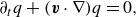(2.2) \begin{equation} \partial _t q + ({\boldsymbol{v}} \cdot \nabla ) q = 0, \end{equation}

which we call the vorticity form of (2.1), and the Biot–Savart law gives

(2.3) \begin{equation} {\boldsymbol{v}}({\boldsymbol{x}},t) = (\boldsymbol{K} \ast q)({\boldsymbol{x}},t) := \int _{{\mathbb R}^2} \boldsymbol{K}({\boldsymbol{x}}- \boldsymbol{y}) q(\boldsymbol{y},t) {\textrm d} \boldsymbol{y}, \qquad \boldsymbol{K}({\boldsymbol{x}}) := \frac {1}{2 \pi }\frac {{\boldsymbol{x}}^\perp }{|{\boldsymbol{x}}|^2}, \end{equation}

where ${\boldsymbol{x}}^\perp := (- x_2, x_1)$ . The initial value problem of (2.2) in ${\mathbb {R}}^2$ has a unique global weak solution for initial vorticity $q_0 \in L^1({\mathbb {R}}^2) \cap L^\infty ({\mathbb {R}}^2)$ (Yudovich 1963). Then, owing to the uniqueness, we have the Lagrangian flow map $\boldsymbol{\eta }$ governed by

(2.4) \begin{equation} \partial _t \boldsymbol{\eta }({\boldsymbol{x}}, t) = {\boldsymbol{v}} \left ( \boldsymbol{\eta }({\boldsymbol{x}}, t), t \right ), \qquad \boldsymbol{\eta }({\boldsymbol{x}}, 0) = {\boldsymbol{x}}. \end{equation}

Note that a unique solution of (2.4) yields a solution of (2.2) via $q({\boldsymbol{x}},t) = q_0(\boldsymbol{\eta }({\boldsymbol{x}}, -t))$ . The existence of a global weak solution to (2.2) has been extended to the case of $q_0 \in L^1({\mathbb {R}}^2) \cap L^p({\mathbb {R}}^2)$ with $p \gt 1$ (DiPerna & Majda 1987) and less regular vorticity $q_0 \in {\mathcal{M}}(\mathbb{R}^2) \cap H_{{loc}}^{-1}(\mathbb{R}^2)$ (Delort 1991; Majda 1993), where ${\mathcal{M}}(\mathbb{R}^2)$ and $H_{{loc}}^{-1}(\mathbb{R}^2)$ denote the space of finite Radon measures and the Sobolev space, respectively.

In this paper, we focus on point-vortex initial vorticity, which is represented by

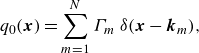(2.5) \begin{equation} q_0({\boldsymbol{x}}) = \sum _{m=1}^N \Gamma _m \ \delta ({\boldsymbol{x}} - \boldsymbol{k}_m), \end{equation}

where $N \in \mathbb{N}$ is the number of point vortices and $\delta ({\boldsymbol{x}})$ is the Dirac delta function. The given constants $\Gamma _m \in {\mathbb {R}} \setminus \{0 \}$ and $\boldsymbol{k}_m \in {\mathbb {R}}^2$ denote the strength and the initial position of the $m$ th point vortex, respectively. Unfortunately, the solvability of (2.2) has not been established for initial vorticity (2.5) in general. In what follows, we formally derive the governing equations of point vortices from (2.2) by assuming that point vortices are convected by the flow map (2.4), and the solution of (2.2) is described by

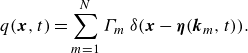(2.6) \begin{equation} q({\boldsymbol{x}},t) = \sum _{m=1}^N \Gamma _m \ \delta ({\boldsymbol{x}} - \boldsymbol{\eta }(\boldsymbol{k}_m,t)). \end{equation}

For simplicity, we set ${\boldsymbol{x}}_m(t) := \boldsymbol{\eta }(\boldsymbol{k}_m,t)$ . Then, (2.4) and the Biot–Savart law yield

(2.7) \begin{equation} \frac {\mbox{d}}{\mbox{d}t} {\boldsymbol{x}}_m(t) = \sum _{n=1}^N \Gamma _n \int \boldsymbol{K} ( {\boldsymbol{x}}_m(t) - \boldsymbol{y})\ \delta (\boldsymbol{y} - {\boldsymbol{x}}_n(t)) {\textrm d}\boldsymbol{y} \sim \sum _{n\neq m}^N \Gamma _n \boldsymbol{K} ({\boldsymbol{x}}_m(t) - {\boldsymbol{x}}_n(t) ). \end{equation}

Note that the last approximation is not a mathematically rigorous calculation but a formal one, since the kernel $\boldsymbol{K}$ is not bounded at the origin. Introducing complex positions of point vortices $z_m(t) := x_m(t) + i y_m(t)$ for convenience of notation, we find the point-vortex (PV) system:

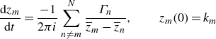(2.8) \begin{equation} \dfrac {\mbox{d} z_m}{\mbox{d}t} = \frac {-1}{2 \pi i} \sum _{n\neq m}^N \dfrac {\Gamma _n}{\overline {z}_m - \overline {z}_n}, \qquad z_m(0) = k_m \end{equation}

for $m = 1,\ldots {\kern-1pt}, N$ , where $\overline {z}_m$ denotes the complex conjugate of $z_m$ and $k_m$ denotes the complex position of $\boldsymbol{k}_m \in \mathbb{R}^2$ . The PV system is formulated as a Hamiltonian dynamical system with the Hamiltonian,

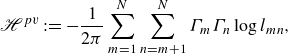(2.9) \begin{equation} {\mathscr{H}}^{{pv}} := - \frac {1}{2 \pi } \sum _{m=1}^{N} \sum _{n=m+1}^{N} \Gamma _{m} \Gamma _{n} \log {l_{mn}}, \end{equation}

where $l_{mn}(t) := |z_m(t) - z_n(t)|$ (Kirchhoff 1876). In addition to the Hamiltonian ${\mathscr{H}}^{{pv}}$ , the PV system has the following invariant quantities:

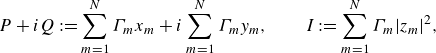(2.10) \begin{align} P + i Q := \sum _{m=1}^N \Gamma _m x_m + i \sum _{m=1}^N \Gamma _m y_m, \qquad I := \sum _{m=1}^N \Gamma _m |z_m|^2, \end{align}

and these quantities yield another invariant,

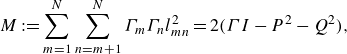(2.11) \begin{equation} M := \sum _{m=1}^N \sum _{n=m+1}^N \Gamma _m \Gamma _n l_{mn}^2 = 2(\Gamma I - P^2 - Q^2), \end{equation}

where $\Gamma := \sum _{m=1}^N \Gamma _m$ . Considering these invariants, we find that the PV system (2.8) with $N \leqslant 3$ is integrable for any $\Gamma _m \in \mathbb{R}\setminus \{0\}$ and the system with $N = 4$ is integrable when $\Gamma = 0$ holds, see Newton (2001) for details. The system is no longer integrable for $N = 4$ with $\Gamma \neq 0$ and $N \geqslant 5$ , for which the dynamics of point vortices could be chaotic.

2.2. Self-similar solutions

Self-similar motions of point vortices are described by the form of

(2.12) \begin{equation} z_m(t) = k_m f(t), \qquad f(t) := r(t) e^{i \theta (t)}, \end{equation}

where $r \geqslant 0$ and $\theta \in \mathbb{R}$ satisfy $r(0) = 1$ and $\theta (0) = 0$ (Kimura 1987). Here, owing to the translational invariance of the PV system, we fix the centre of point vortices to the origin, that is, $P=Q=0$ . Substituting (2.12) into (2.8), we find

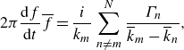(2.13) \begin{equation} 2 \pi \dfrac {\mbox{d}f}{\mbox{d}t} \overline {f} = \frac {i}{k_m} \sum _{n\neq m}^N \dfrac {\Gamma _n}{\overline {k}_m - \overline {k}_n}, \end{equation}

which implies that the existence of a self-similar solution is equivalent to the existence of an initial configuration $\{ k_m \}_{m=1}^N$ for which there exist constants $A$ , $B \in \mathbb{R}$ independent of $m$ such that they satisfy

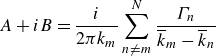(2.14) \begin{equation} A + i B = \frac {i}{2 \pi k_m} \sum _{n\neq m}^N \dfrac {\Gamma _n}{\overline {k}_m - \overline {k}_n} \end{equation}

for any $m = 1,\ldots {\kern-1pt},N$ . See Gotoda (2021) for the explicit formulae of the constants $A$ and $B$ . For the case of $A \neq 0$ , the self-similar solution of the PV system is explicitly described by

(2.15) \begin{equation} z_m(t) = k_m \sqrt {2At + 1} \exp {\left [ i \dfrac {B}{2A}\log {(2At + 1)} \right ]}, \quad m = 1,\ldots {\kern-1pt},N, \end{equation}

and the mutual distances are given by $l_{mn}(t) = l_{mn}(0) \sqrt {2At + 1}$ for $m \neq n$ (Kimura 1987). Thus, the point vortices simultaneously collide at the origin with the time

(2.16) \begin{equation} t_c := - \frac {1}{2A}, \end{equation}

which is called the collapse time. We call self-similar motions with $A \lt 0$ collapsing and those with $A \gt 0$ expanding in the positive direction of time. For the initial position satisfying $A =0$ , the corresponding self-similar solution is a relative equilibrium in the form $z_m(t) = k_m e^{i B t}$ that rotates rigidly about their centre of vorticity with the angular velocity $B$ . It is easily confirmed that self-similar solutions with $A \neq 0$ satisfy $I = M = 0$ and

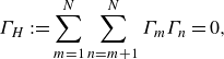(2.17) \begin{equation} \Gamma _H := \sum _{m=1}^N \sum _{n=m+1}^N \Gamma _m \Gamma _n = 0, \end{equation}

which follows from the invariance of the Hamiltonian. Note that we may fix the $N$ th point vortex of the initial configuration to $z_N = 1$ on the real axis since the PV system has rotational and scaling invariance.

2.3. Exact solutions for self-similar collapse

In the three-PV system, it is known that $\Gamma _H = M = 0$ is a necessary and sufficient condition for the self-similar collapse (Aref 1979; Kimura 1987; Newton 2001), and any partial collapse does not occur. Note that $\Gamma _H = 0$ allows us to assume that $\Gamma _1$ , $\Gamma _2$ have a same sign and $\Gamma _3$ does the opposite one without loss of generality: $\Gamma _3$ is replaced by $ - \Gamma _1 \Gamma _2 /(\Gamma _1 + \Gamma _2)$ . Under the condition $\Gamma _H = M = 0$ , initial configurations of self-similar solutions are expressed by

(2.18) \begin{equation} k_1 = \dfrac {\Gamma _1 \Gamma _2}{(\Gamma _1 + \Gamma _2)^2} \left ( 1 - \dfrac {\sqrt {\mathcal{R}}}{\Gamma _1} e^{i \theta } \right ), \quad k_2 = \dfrac {\Gamma _1 \Gamma _2}{(\Gamma _1 + \Gamma _2)^2} \left ( 1 + \dfrac {\sqrt {\mathcal{R}}}{\Gamma _2} e^{i \theta } \right ), \quad k_3 = 1 \end{equation}

for $\theta \in [0, 2\pi )$ , where $\mathcal{R} := \Gamma _1^2 + \Gamma _1 \Gamma _2 + \Gamma _2^2$ , see Kimura (1987). Then, three point vortices form equilateral triangles for $\theta = \theta _\pm$ satisfying $\cos {\theta _\pm } = - (\Gamma _1 - \Gamma _2)/(2 \sqrt {\mathcal{R}})$ and $0 \lt \theta _+ \lt \pi \lt \theta _- \lt 2\pi$ . Since the initial configuration (2.18) is a one-parameter family with the parameter $\theta \in [0,2 \pi )$ , ${\mathscr{H}}$ and $(A, B)$ in (2.14) are considered as functions of $\theta$ , see Newton (2001)and Gotoda (2021) for the explicit formulae of them. All possible equilibria, which are equivalent to $A = 0$ , are collinear states for $\theta = 0, \pi$ and equilateral triangles for $\theta = \theta _\pm$ . It is easily confirmed that the self-similar solution is collapsing for $\theta \in (0, \theta _+) \cup (\pi , \theta _-)$ and expanding for $\theta \in (\theta _+, \pi ) \cup (\theta _-, 2 \pi )$ . In the case of $\Gamma _1 = \Gamma _2$ , which is the case we use for numerical computations later, we have $\theta _+ = \pi /2$ and $\theta _- = 3 \pi /2$ .

In the PV system with $N \geqslant 4$ , explicit formulae for configurations leading to self-similar collapse have not been established in general. However, an example of exact self-similar collapsing solutions for the four- and five-vortex problems has been obtained by Novikov & Sedov (1979). In this example, four point vortices are located at vertices of a parallelogram whose diagonals intersect at the origin and the fifth point vortex is located at the origin, that is,

(2.19) \begin{equation} k_1 = \dfrac {1}{2} d_1 e^{i\theta }, \qquad k_2 = - \dfrac {1}{2} d_1 e^{i\theta }, \qquad k_3 = - \dfrac {1}{2} d_2, \qquad k_4 = \dfrac {1}{2} d_2, \qquad k_5 = 0, \end{equation}

where given constants $d_1, d_2$ are lengths of the diagonals and $\theta \in [0,2\pi )$ is the angle between the diagonals. The strengths of point vortices are $\Gamma _1 = \Gamma _2 = \alpha$ , $\Gamma _3 = \Gamma _4 = \beta$ and $\Gamma _5 = \gamma$ , where $\alpha , \beta , \gamma \in \mathbb{R} \setminus \{ 0 \}$ are given constants. The configuration (2.19) satisfies $P = Q = 0$ and, due to the self-similarity with rotation, we have

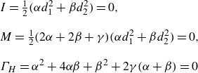(2.20) \begin{equation} \begin{aligned} & I = \tfrac {1}{2}\Big( \alpha d_1^2 + \beta d_2^2 \Big) = 0, \\[8pt] & M = \tfrac {1}{2}(2 \alpha + 2 \beta + \gamma )\Big( \alpha d_1^2 + \beta d_2^2 \Big) = 0, \\[8pt] & \Gamma _H = \alpha ^2 + 4 \alpha \beta + \beta ^2 + 2 \gamma (\alpha + \beta )= 0 \end{aligned} \end{equation}

and these conditions yield the relation $d_1^2 / d_2^2 = - \beta /\alpha$ . Ignoring the fifth point vortex $k_5$ , we have the initial configuration leading to self-similar collapse for the four-PV system. Similarly to the five-PV problem, we have $P = Q = 0$ and (2.20) with $\gamma \equiv 0$ should be satisfied. Then, we have $d_1^2 / d_2^2 = - \beta /\alpha = 2 \pm \sqrt {3} \gt 0$ . Considering (2.19) as a one-parameter family, the Hamiltonian ${\mathscr{H}}^{{pv}}$ is represented by

(2.21) \begin{equation} {\mathscr{H}}^{{pv}}(\theta ) = \dfrac {-1}{2 \pi } \log {\left[ c_H d_1^{\alpha (\alpha + 2 \gamma )} d_2^{\beta (\beta + 2 \gamma )} \Big(d_1^4 + d_2^4 - 2 d_1^2 d_2^2 \cos {2 \theta } \Big)^{\alpha \beta } \right]}, \end{equation}

where $c_H := 2^{ -4 \alpha \beta - 2 \gamma (\alpha + \beta )}$ , and this formula is valid for the four-vortex problem by setting $\gamma \equiv 0$ . The explicit formulae for $(A,B)$ in (2.14) for (2.19) have been obtained as functions of $\theta$ , see Novikov & Sedov (1979). In both the four- and five-PV systems, relative equilibria are diamond configurations for $\theta = \pi /2, 3\pi /2$ and collinear states for $\theta = 0, \pi$ . In this paper, we consider the case of $\alpha \lt 0$ , for which the self-similar motions are collapsing for $\theta \in (0, \pi /2) \cup (\pi , 3\pi /2)$ and expanding for $\theta \in (\pi /2, \pi ) \cup (3\pi /2, 2\pi )$ .

3. The filtered point-vortex system

3.1. Dynamics of point vortices on the 2-D filtered-Euler flow

We introduce the filtered-point-vortex (FPV) system, which describes the dynamics of point-vortex solutions of the 2-D filtered-Euler equations. The filtered-Euler equations are a regularised model of the Euler equations on the basis of a spatial filtering and given by

(3.1) \begin{equation} \partial _t {\boldsymbol{v}}^\varepsilon + (\boldsymbol{u}^\varepsilon \cdot \nabla ){\boldsymbol{v}}^\varepsilon - (\nabla {\boldsymbol{v}}^\varepsilon )^T \cdot \boldsymbol{u}^\varepsilon - \nabla p^\varepsilon = 0, \quad \boldsymbol{u}^\varepsilon = h^\varepsilon \ast {\boldsymbol{v}}^\varepsilon , \quad \nabla \cdot {\boldsymbol{v}}^\varepsilon = 0, \end{equation}

where ${\boldsymbol{v}}^\varepsilon$ and $p^\varepsilon$ are unknown functions, and $h^\varepsilon$ has the form

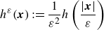(3.2) \begin{align} h^\varepsilon ({\boldsymbol{x}}) := \frac {1}{\varepsilon ^2} h \left ( \frac {|{\boldsymbol{x}}|}{\varepsilon } \right ) \end{align}

with a given filter function $h \in L^1(0,\infty )$ (Foias et al. 2001; Holm et al. 2006). We mention detailed properties that a filter function $h$ should satisfy in Remark 2. We consider the vorticity $q^\varepsilon := \operatorname {curl} {\boldsymbol{v}}^\varepsilon$ and the vorticity form of (3.1):

(3.3) \begin{equation} \partial _t q^\varepsilon + (\boldsymbol{u}^\varepsilon \cdot \nabla )q^\varepsilon = 0, \qquad \boldsymbol{u}^\varepsilon = \boldsymbol{K}^\varepsilon \ast q^\varepsilon , \end{equation}

where $\boldsymbol{K}^\varepsilon := \boldsymbol{K} \ast h^\varepsilon$ is a filtered kernel and we call the relation $\boldsymbol{u}^\varepsilon = \boldsymbol{K}^\varepsilon \ast q^\varepsilon$ the filtered-Biot–Savart law. In contrast to the 2-D Euler equations, the 2-D filtered-Euler equations have a unique global weak solution for initial vorticity $q_0 \in {\mathcal{M}}({\mathbb {R}}^2)$ (Gotoda 2018), which guarantees the global solvability for the point-vortex initial data (2.5). Thus, we have the filtered-Lagrangian flow map $\boldsymbol{\eta }^\varepsilon$ convected by the filtered velocity $\boldsymbol{u}^\varepsilon$ :

(3.4) \begin{equation} \partial _t \boldsymbol{\eta }^\varepsilon ({\boldsymbol{x}}, t) = \boldsymbol{u}^\varepsilon \left ( \boldsymbol{\eta }^\varepsilon ({\boldsymbol{x}}, t), t \right ), \qquad \boldsymbol{\eta }^\varepsilon ({\boldsymbol{x}}, 0) = {\boldsymbol{x}}, \end{equation}

and the solution of (3.3) is expressed by $q^\varepsilon ({\boldsymbol{x}},t) = q_0(\boldsymbol{\eta }^\varepsilon ({\boldsymbol{x}}, -t))$ . The convergence of the 2-D filtered-Euler equations to the 2-D Euler equations has been proven for the initial vorticity in $L^1({\mathbb {R}}^2) \cap L^p({\mathbb {R}}^2)$ with $1 \lt p \leqslant \infty$ and ${\mathcal{M}}(\mathbb{R}^2) \cap H_{{loc}}^{-1}(\mathbb{R}^2)$ , see Gotoda (2018, 2020).

Remark 1. The singular kernel $\boldsymbol{K}$ appearing in the 2-D Euler equations is expressed by $\boldsymbol{K} = \nabla ^\perp G$ , where $\nabla ^\perp = (- \partial _{x_2}, \partial _{x_1})$ and $G$ is a fundamental solution to the 2-D Laplacian $\Delta G = \delta$ . The filtered kernel $\boldsymbol{K}^\varepsilon$ in the 2-D filtered-Euler equations is represented by $\boldsymbol{K}^\varepsilon = \nabla ^\perp G^\varepsilon$ , where $G^\varepsilon$ is a solution to the 2-D Poisson equation $\Delta G^\varepsilon = h^\varepsilon$ . Since $h^\varepsilon$ is radially symmetric, it is easily confirmed that $\boldsymbol{K}^\varepsilon ({\boldsymbol{x}}) = \nabla ^\perp (G_r (|{\boldsymbol{x}}|/ \varepsilon ) )$ and $G_r$ satisfies

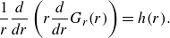(3.5) \begin{equation} \frac {1}{r} \frac {{d}}{{{d}}r} \left ( r \frac {{{d}}}{{d}r} G_r(r) \right ) = h(r). \end{equation}

Then, we have

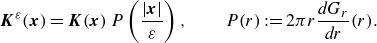(3.6) \begin{equation} \boldsymbol{K}^\varepsilon ({\boldsymbol{x}}) = \boldsymbol{K}({\boldsymbol{x}})\, P\left ( \frac {|{\boldsymbol{x}}|}{\varepsilon } \right ), \qquad P(r) := 2\pi r \frac {{{d}} G_r}{{d}r}(r). \end{equation}

The function $P \in C[0,\infty )$ is monotonically increasing and satisfies $P(0)=0$ and $P(r) \to 1$ as $r \to \infty$ . Note that $\boldsymbol{K}^\varepsilon$ does not have singularity at the origin and belongs to $C_0({\mathbb {R}}^2)$ , the space of continuous functions vanishing at infinity.

We consider point-vortex solutions of (3.3). Owing to the uniqueness for the initial vorticity (2.5), we have a unique filtered-Lagrangian flow map $\boldsymbol{\eta }^\varepsilon$ and the solution of (3.3) is given by

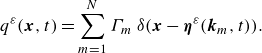(3.7) \begin{equation} q^\varepsilon ({\boldsymbol{x}},t) = \sum _{m=1}^N \Gamma _m \ \delta ({\boldsymbol{x}} - \boldsymbol{\eta }^\varepsilon (\boldsymbol{k}_m,t)). \end{equation}

Setting ${\boldsymbol{x}}^\varepsilon _m(t) := \boldsymbol{\eta }^\varepsilon (\boldsymbol{k}_m,t)$ , we find from (3.4) and the filtered-Biot–Savart law that

(3.8) \begin{equation}{d \over {dt}} {\boldsymbol{x}}^\varepsilon _m(t) = \sum _{n=1}^N \Gamma _n \int \boldsymbol{K}^\varepsilon \big( {\boldsymbol{x}}^\varepsilon _m(t) - \boldsymbol{y}\big)\ \delta \big(\boldsymbol{y} - {\boldsymbol{x}}^\varepsilon _n(t)\big) \,{\textrm d}\boldsymbol{y} = \sum _{n\neq m}^N \Gamma _n \boldsymbol{K}^\varepsilon \big({\boldsymbol{x}}^\varepsilon _m(t) - {\boldsymbol{x}}^\varepsilon _n(t)\big). \end{equation}

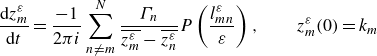
Let $z_m^\varepsilon (t) := x_m^\varepsilon (t) + i y_m^\varepsilon (t)$ and recall (3.6). Then, we obtain the FPV system in the complex form:

(3.9) \begin{equation} \dfrac {\mbox{d} z_m^\varepsilon }{\mbox{d}t} = \frac {-1}{2 \pi i} \sum _{n\neq m}^N \dfrac {\Gamma _n}{\overline {z_m^\varepsilon } - \overline {z_n^\varepsilon }} P\left ( \frac {l_{mn}^\varepsilon }{\varepsilon } \right ), \qquad z_m^\varepsilon (0) = k_m \end{equation}

for $m = 1,\ldots {\kern-1pt}, N$ , where $l_{mn}^\varepsilon (t) := |z_m^\varepsilon (t) - z_n^\varepsilon (t)|$ , see Gotoda & Sakajo (2018). We call point vortices governed by the FPV system filtered point vortices. The FPV system is a Hamiltonian system with the Hamiltonian

(3.10) \begin{equation} {\mathscr{H}}^\varepsilon := - \frac {1}{2 \pi } \sum _{m=1}^N \sum _{n=m+1}^N \Gamma _m \Gamma _n \left [ \log {l_{mn}^\varepsilon } + H_G\left ( \frac {l_{mn}^\varepsilon }{\varepsilon } \right ) \right ], \end{equation}

where $H_G(r) := - \log {r} + 2 \pi G_r(r)$ . The FPV system admits the conserved quantities $(P^\varepsilon , Q^\varepsilon , I^\varepsilon , M^\varepsilon )$ , which are defined in the same manner as $(P, Q, I, M)$ in the PV system, and ${\mathscr{H}}^\varepsilon$ . The integrability of (3.9) depending on $N$ is also same as the PV system.

It is important to remark that, owing to the global solvability and uniqueness, filtered point vortices never collapse for any $\varepsilon \gt 0$ . In contrast to the 2-D Euler equations, the derivation of (3.9) is mathematically rigorous and thus the FPV system is equivalent to the vorticity form of the 2-D filtered-Euler equations with initial data (2.5): a weak solution to the 2-D filtered-Euler equations yields a solution to the FPV system and vice versa.

Remark 2. The filter function $h$ characterises the regularity of the filtered model. In this paper, we suppose that $h$ is a given function satisfying $h \in C_0(0, \infty ) \cap L^1(0,\infty )$ and

(3.11) \begin{equation} 2 \pi \int _0^\infty r h (r)\, {\textrm d}r = 1. \end{equation}

Note that $h$ may have a singularity at the origin but should decay at infinity, see Gotoda (2018)and Gotoda & Sakajo (2018) for the detailed condition that guarantees the global solvability for the point-vortex initial vorticity. For a suitable filter function $h$ , the 2-D filtered-Euler equations have a unique global weak solution for initial vorticity in ${\mathcal{M}}({\mathbb {R}}^2)$ . Considering a specific filter function $h$ , we obtain an explicit form of the filtered-Euler equations. For instance, the Euler- $\alpha$ model, the vortex blob regularisation and the exponential model are often used as a regularised inviscid model.

3.2. Variations of enstrophy and energy

We introduce variations of the enstrophy and the energy for solutions to the FPV system. The derivations of them are based on the Fourier transform and we here start with the final forms of the total enstrophy and the approximated total energy, see Gotoda & Sakajo (2018) for the detailed derivations. We define the total enstrophy by the $L^2$ -norm of the filtered vorticity $\omega ^\varepsilon := h^\varepsilon \ast q^\varepsilon$ . Then, the total enstrophy of the FPV system is given by

(3.12) \begin{equation} \begin{aligned} \frac {1}{2}\int _{\mathbb{R}^2} \left \vert \omega ^\varepsilon ({\boldsymbol x}, t) \right \vert ^2 \,{\textrm d}{\boldsymbol x} &= \frac {1}{4 \pi \varepsilon ^2} \sum _{m=1}^N \Gamma _m^2 \int _0^\infty s \left \vert 2\pi \widehat {h}(s) \right \vert ^2\, {\textrm d}s \\[8pt] &\quad + \frac {1}{2\pi \varepsilon ^2} \sum _{m=1}^N \sum _{n=m+1}^N \Gamma _m \Gamma _n \int _0^\infty s \left \vert 2\pi \widehat {h}(s) \right \vert ^2 J_0 \left ( s \frac {l_{mn}^\varepsilon }{\varepsilon } \right ) \,{\textrm d}s, \end{aligned} \end{equation}

where $\widehat {h}$ is the Fourier transform of $h$ and $J_0$ is the zeroth-order Bessel function of the first kind. The first term in the right-hand side describes the enstrophy produced by self-interaction of point vortices and the second one comes from interaction among separated point vortices. Since the self-interaction term is constant in time and diverges to infinity in the $\varepsilon \to 0$ limit, we consider the variational part of the total enstrophy provided by the second term,

(3.13) \begin{equation} {\mathscr{Z}}^\varepsilon (t) := \frac {1}{2\pi \varepsilon ^2} \sum _{m=1}^N \sum _{n=m+1}^N \Gamma _m \Gamma _n \int _0^\infty s \left \vert 2\pi \widehat {h}(s) \right \vert ^2 J_0 \left ( s \frac {l_{mn}^\varepsilon (t)}{\varepsilon } \right ) \,{\textrm d}s, \end{equation}

and investigate how the enstrophy varies with mutual interaction of point vortices. In what follows, we call the variation ${\mathscr{Z}}^\varepsilon$ the enstrophy of the FPV system. The total energy for the filtered model is defined by the $L^2$ -norm of the filtered velocity $\boldsymbol{u}^\varepsilon$ . However, the total energy on the whole space ${\mathbb {R}}^2$ is not finite in general, since the filtered-Biot–Savart law implies $\boldsymbol{u}^\varepsilon ({\boldsymbol{x}}) \sim |{\boldsymbol{x}}|^{-1}$ as $|{\boldsymbol{x}}| \to \infty$ . Thus, we consider the total energy cut off at a scale larger than $L \gg 1$ . Then, the following approximation holds:

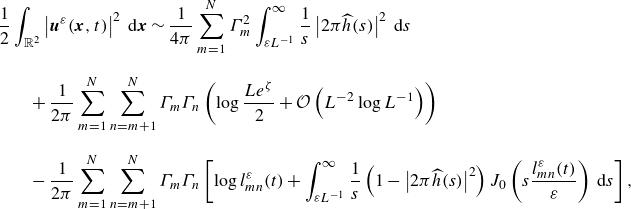(3.14) \begin{align} \frac {1}{2} & \int _{\mathbb{R}^2} \left \vert {\boldsymbol u}^\varepsilon ({\boldsymbol x}, t) \right \vert ^2\, {\textrm d}{\boldsymbol x} \sim \frac {1}{4 \pi } \sum _{m=1}^N \Gamma _m^2\int _{\varepsilon L^{-1}}^\infty \frac {1}{s} \left \vert 2\pi \widehat {h}(s) \right \vert ^2 \,{\textrm d}s \nonumber \\[8pt] & \quad + \frac {1}{2\pi } \sum _{m=1}^N \sum _{n=m+1}^N \Gamma _m \Gamma _n \left ( \log {\frac {L e^\zeta }{2}} + \mathcal{O}\left ( L^{-2} \log {L^{-1}} \right ) \right ) \nonumber \\[8pt] & \quad - \frac {1}{2\pi } \sum _{m=1}^N \sum _{n=m+1}^N \Gamma _m \Gamma _n \left [ \log {l_{mn}^\varepsilon (t)} + \int _{\varepsilon L^{-1}}^\infty \frac {1}{s} \left ( 1 - \left \vert 2\pi \widehat {h}(s) \right \vert ^2 \right ) J_0 \left ( s \frac {l_{mn}^\varepsilon (t)}{\varepsilon } \right ) \,{\textrm d}s \right ], \end{align}

where $\zeta$ is Euler’s constant. Taking the $L \rightarrow \infty$ limit in the non-constant part, we obtain a variational part of the approximated total energy:

(3.15) \begin{equation} {\mathscr{E}}^\varepsilon (t) := - \frac {1}{2\pi } \sum _{m=1}^N \sum _{n=m+1}^N \! \Gamma _m \Gamma _n \! \left [ \log {l_{mn}^\varepsilon (t)} + \!\int _0^\infty \frac {1}{s} \left ( 1 - \left \vert 2\pi \widehat {h}(s) \right \vert ^2 \right ) J_0 \left ( s \frac {l_{mn}^\varepsilon (t)}{\varepsilon } \right ) {\textrm d}s \right ], \end{equation}

in which the integrand of the second term does not have any singularity owing to $2\pi \widehat {h}(0) = 1$ . Then, we define the energy dissipation rate of the FPV system by the time derivative of ${\mathscr{E}}^\varepsilon (t)$ :

(3.16) \begin{equation} {\mathscr{D}}_E^\varepsilon (t) := \frac {\mbox{d}}{\mbox{d} t} {\mathscr{E}}^\varepsilon (t). \end{equation}

3.3. Preceding results about enstrophy dissipation

As the first attempt of constructing a point-vortex solution dissipating the enstrophy, Sakajo (2012) has numerically shown that self-similar collapse of three point vortices could dissipate the enstrophy by using the Euler- $\alpha$ model. Let us review the preceding results for the Euler- $\alpha$ model more precisely since we use this model later for numerical computations. In the Euler- $\alpha$ model, the filter function $h$ is given by

(3.17) \begin{equation} h(r) = \frac {1}{2 \pi } K_0(r), \end{equation}

where $K_0$ is the zeroth-order modified Bessel function of the second kind, for which the corresponding equations (3.1) are called the 2-D Euler- $\alpha$ equations. Then, we find that the smoothing function $P$ in the FPV system (3.9) is expressed by

(3.18) \begin{equation} P(r) = 1 - r K_1(r), \end{equation}

where $K_1$ denotes the first-order modified Bessel function of the second kind, see Gotoda & Sakajo (2016a , b ) and Sakajo (2012). The FPV system and filtered point vortices with (3.18) are called the $\alpha$ -point-vortex ( $\alpha$ PV) system and $\alpha$ -point vortices, respectively. Note that the filter parameter in the Euler- $\alpha$ model is often denoted by $\alpha$ , but we consistently use $\varepsilon$ to avoid confusion in this paper. The quantities ${\mathscr{H}}^\varepsilon$ , ${\mathscr{Z}}^\varepsilon$ and ${\mathscr{E}}^\varepsilon$ for the $\alpha$ -PV system are explicitly described by

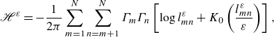(3.19a) \begin{align} {\mathscr{H}}^\varepsilon &= - \frac {1}{2 \pi } \sum _{m=1}^N \sum _{n=m+1}^N \Gamma _m \Gamma _n \left [ \log {l_{mn}^\varepsilon } + K_0\left ( \frac {l_{mn}^\varepsilon }{\varepsilon } \right ) \right ], \end{align}

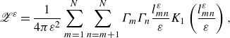(3.19b) \begin{align} {\mathscr{Z}}^\varepsilon &= \frac {1}{4\pi \varepsilon ^2} \sum _{m=1}^N \sum _{n=m+1}^N \Gamma _m \Gamma _n \frac {l_{mn}^\varepsilon }{\varepsilon } K_1 \left ( \frac {l_{mn}^\varepsilon }{\varepsilon } \right ), \end{align}

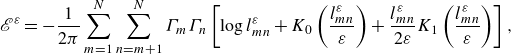(3.19c) \begin{align} {\mathscr{E}}^\varepsilon &= - \frac {1}{2\pi } \sum _{m=1}^N \sum _{n=m+1}^N \Gamma _m \Gamma _n \left [ \log {l_{mn}^\varepsilon } + K_0 \left ( \frac {l_{mn}^\varepsilon }{\varepsilon } \right ) + \frac {l_{mn}^\varepsilon }{2 \varepsilon } K_1 \left ( \frac {l_{mn}^\varepsilon }{\varepsilon } \right ) \right ],\end{align}

and they satisfy ${\mathscr{E}}^\varepsilon + \varepsilon ^2 {\mathscr{Z}}^\varepsilon = {\mathscr{H}}^\varepsilon$ . Sakajo (2012) has considered the three- $\alpha$ -PV system and shown with the help of numerical computations that, under the condition $\Gamma _H = M ^\varepsilon = 0$ , three $\alpha$ -point vortices converge to a self-similar collapsing solution of the PV system in the $\varepsilon \to 0$ limit and dissipate the enstrophy at the event of the triple collapse while the energy is conserved. Subsequently, this result has been proven with mathematical rigour by Gotoda & Sakajo (2016b ) and then Gotoda & Sakajo (2018) have proven that the same result holds for the FPV system (3.9) with the general filter function $h$ . In these preceding studies, the enstrophy dissipation by collapse of point vortices and the energy conservation mean that there exist constants $t_c \in {\mathbb {R}}$ and $m_z \lt 0$ such that we have

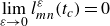(3.20) \begin{equation} \lim _{\varepsilon \rightarrow 0} l^\varepsilon _{mn}(t_c) = 0 \end{equation}

for any $m \neq n$ , and

(3.21) \begin{equation} \lim _{\varepsilon \rightarrow 0} {\mathscr{Z}}^\varepsilon = m_z \delta (\cdot - t_c) , \qquad \lim _{\varepsilon \rightarrow 0} {\mathscr{D}}_E^\varepsilon = 0 \end{equation}

in the sense of distributions. Here, $t_c$ is the time when the self-similar collapse occurs and $m_z$ is the mass of the enstrophy dissipation. For the $N$ vortex problem with $N \geqslant 4$ , we have one numerical example of quadruple collapse causing the enstrophy dissipation in the four- $\alpha$ -PV system of Gotoda & Sakajo (2016a ) with specific initial data that is also found numerically. In the present study, we consider the four- and five-vortex problems in the FPV system for the one-parameter family of initial data (2.19) and give numerical solutions leading to the enstrophy dissipation by vortex collapse in the $\varepsilon \to 0$ limit.

Remark 3. The preceding studies have also shown that three filtered-point vortices converge to a self-similar collapsing solution to the three-PV system with the collapse time $t_c$ . Although the filtered-point vortices exist globally in time for $\varepsilon \gt 0$ , the $\varepsilon \to 0$ limit of them is no longer defined at $t = t_c$ and we cannot connect the two limit solutions for $t \lt t_c$ and $t \gt t_c$ at the collapse time. As we see in § 4 , the enstrophy for the filtered-point vortices with $\varepsilon \gt 0$ decreases to minimum at the critical time and then returns to the original value as time evolves. However, in the $\varepsilon \to 0$ limit, the minimum value of the enstrophy diverges to negative infinity at the collapse time. Therefore, the $\varepsilon \to 0$ limit solution of the FPV system exists in the time interval $(-\infty ,t_c)$ and breaks down at $t = t_c$ with the divergence of the enstrophy, which holds for the limit solution for $t \gt t_c$ , that is, it exists in $(t_c, \infty )$ and the enstrophy diverges at $t = t_c$ as time evolves in the negative direction.

4. Main results

4.1. Numerical method

To conduct numerical computations for dynamics of solutions to the FPV system, we have to give an explicit filter function $h$ . In this paper, we employ the $\alpha$ -PV system, that is, the FPV system (3.9) with (3.17), and consider the three-, four- and five-vortex problems: the three- $\alpha$ -PV system with (2.18), the four- $\alpha$ -PV system with (2.19) without $k_5$ and the five- $\alpha$ -PV system with (2.19). Similarly to the PV system, solutions to the FPV system for $\theta \in (\pi , 2\pi )$ are symmetric to those for $\theta \in (0, \pi )$ with the real axis. In addition, solutions for $\theta \in (\pi /2, \pi )$ are expanding and thus there is no collapse of filtered point vortices in the $\varepsilon \to 0$ limit for any positive time. For the cases of $\theta = 0, \pi /2, \pi$ and $3\pi /2$ on the axes, as we mentioned in § 2.3, the corresponding solutions to the PV system are relative equilibria. However, the solutions to the FPV system for those initial configurations are not relative equilibria and they are expanding, except for the three filtered-point vortices with $\theta = \pi /2$ . Thus, it is enough to pay attention to $\theta \in (0, \pi /2)$ for considering the enstrophy dissipation by vortex collapse.

For later use, we introduce several notation. Since solutions to the FPV system are parametrised by $\theta$ in the initial data (2.18) and (2.19), we describe

(4.1) \begin{equation} l_{mn}^\varepsilon (t;\theta ) = l_{mn}^\varepsilon (t) \end{equation}

when we emphasise that the solutions depend on $\theta$ . Then, for $\theta \in (0,\pi /2)$ , we define the critical time $t_c^\varepsilon = t_c^\varepsilon (\theta )$ as the time when the total length of $l_{mn}^\varepsilon$ in the $L^2$ -sense,

(4.2) \begin{equation} L^\varepsilon (t; \theta ) := \sum _{m =1}^N \sum _{n = m + 1}^N \left ( l^\varepsilon _{mn}(t;\theta ) \right )^2, \end{equation}

attains its minimum, that is,

(4.3) \begin{equation} t_c^\varepsilon = t_c^\varepsilon (\theta ) := \underset {t \geqslant 0}{\operatorname {argmin}}\ L^\varepsilon (t; \theta ). \end{equation}

The critical time $t_c^\varepsilon$ corresponds to the collapse time of the PV system. Indeed, for initial data (2.18) and (2.19), the collapse time (2.16) of the PV system is a function of $\theta$ , which we describe by

(4.4) \begin{equation} t_c = t_c(\theta ) := \frac {1}{2 A(\theta )}, \end{equation}

where $A(\theta )$ is given by (2.14). Then, as we see later, numerical computations show that $t_c^\varepsilon (\theta )$ converges to $t_c(\theta )$ in the $\varepsilon \to 0$ limit for any $\theta \in (0, \pi /2)$ . The enstrophy ${\mathscr{Z}}^\varepsilon$ and the energy dissipation rate ${\mathscr{D}}_E^\varepsilon$ are also functions of $\theta$ and denoted by ${\mathscr{Z}}^\varepsilon (t; \theta )$ and ${\mathscr{D}}^\varepsilon _E(t; \theta )$ . In particular, we represent the values of $L^\varepsilon (t; \theta )$ and ${\mathscr{Z}}^\varepsilon (t; \theta )$ at the critical time by

(4.5) \begin{equation} L^\varepsilon _c(\theta ) := L^\varepsilon (t_c^\varepsilon (\theta ), \theta ), \qquad {\mathscr{Z}}^\varepsilon _c(\theta ) := {\mathscr{Z}}^\varepsilon (t_c^\varepsilon (\theta ), \theta ) \end{equation}

for simplicity. We remark that the convergence of $L^\varepsilon _c(\theta )$ to zero and the divergence of ${\mathscr{Z}}^\varepsilon _c(\theta )$ to negative infinity in the $\varepsilon \to 0$ limit indicate collapse of point vortices and the enstrophy dissipation, respectively.

For numerical computations, we divide the interval $(0, \pi /2)$ into $200$ segments and compute solutions to the $\alpha$ -PV system with the initial configuration for

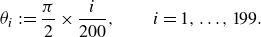(4.6) \begin{equation} \theta _i := \frac {\pi }{2} \times \frac {i}{200}, \qquad i = 1, \ldots {\kern-1pt}, 199. \end{equation}

As for the filter parameter $\varepsilon$ , we compute the five cases of

(4.7) \begin{equation} \varepsilon _1 := 0.01, \quad \varepsilon _2 := 0.025, \quad \varepsilon _3 := 0.05, \quad \varepsilon _4 := 0.075, \quad \varepsilon _5 := 0.1. \end{equation}

As the numerical scheme for solving the $\alpha$ -PV systems, we use the five-stage implicit Runge–Kutta method based on the n-point Gauss–Legendre quadrature formula (Butcher 1964) with the time step size $\Delta t = 0.0001$ . To ensure the accuracy of numerical solutions, we use variables with 32 decimal digit precision. For the four- $\alpha$ -PV system with several initial configurations near $\theta = 0$ , we have used $\Delta t = 0.00001$ and 50 decimal digit precision to accurately compute long time behaviours of the solutions. For the five- $\alpha$ -PV system, mathematical analysis shows that the fifth point vortex is fixed to the origin throughout time evolution and thus we have fixed it in the numerical scheme. Figure 1 shows examples of the four and five $\alpha$ -point vortices for the initial data (2.19) with $\theta = \theta _{30}$ .

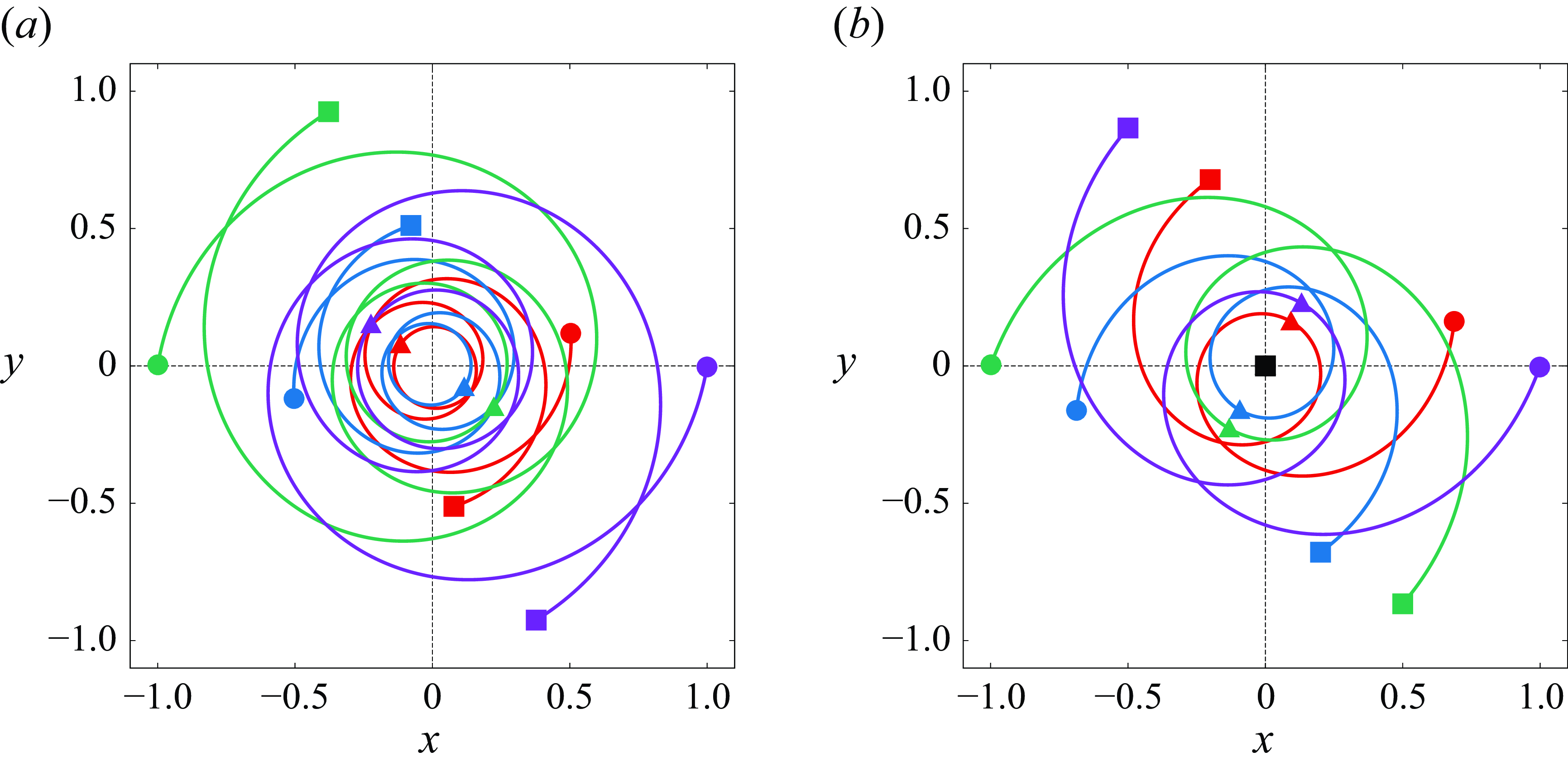
Figure 1. Orbits of the (a) four and (b) five $\alpha$ -point vortices for the initial data (2.19) with $\theta = \theta _{30}$ and the filter parameter $\varepsilon _3 = 0.05$ . The circular, triangle and square points describe the configurations at $t=0$ , $t=t_c^\varepsilon$ and $t=2t_c^\varepsilon$ , respectively.

4.2. Three-vortex problem

In the three-vortex problem, it has already been proven that the solution to the FPV system with initial data (2.18) for $\theta \in (0, \pi /2)$ converges to a self-similar collapsing solution of the PV system and dissipates the enstrophy at the collapse time. However, its mathematical analysis has not revealed the detailed process of the enstrophy dissipation by collapse of three point vortices. To see the convergence process of the filtered-point vortices up to collapse and the associated enstrophy variation as $\varepsilon$ decreases precisely, we investigate the three- $\alpha$ -PV system with initial data (2.18) by numerical computations.

For simplicity, we consider the case of $\Gamma _1 = \Gamma _2$ : we may set $\Gamma _1 = \Gamma _2 = -1$ and $\Gamma _3 = 1/2$ without loss of generality. Then, (2.18) is expressed by

(4.8) \begin{equation} k_1 = \dfrac {1}{4}\left ( 1 + \sqrt {3} e^{i\theta } \right ), \qquad k_2 = \dfrac {1}{4}\left ( 1 - \sqrt {3} e^{i\theta } \right ), \qquad k_3 = 1 \end{equation}

for $\theta \in (0, \pi /2)$ . Figures 2(a) and 2(b) show the graphs of $L^{\varepsilon _3}(t;\theta _i)$ and ${\mathscr{Z}}^{\varepsilon _3}(t; \theta _i)$ for $i = 20, 40, 70, 120, 180$ . These graphs indicate that, for any fixed $\theta \in (0, \pi /2)$ , the functions $L^\varepsilon (t;\theta )$ and ${\mathscr{Z}}^\varepsilon (t;\theta )$ of the variable $t$ are monotonically decreasing for $t \lt t_c^\varepsilon$ and increasing for $t \gt t_c^\varepsilon$ : ${\mathscr{Z}}^\varepsilon (t;\theta )$ attains its minimum at $t_c^\varepsilon (\theta )$ that is defined by the time when $L^\varepsilon (t;\theta )$ reaches its minimum. That is to say, three $\alpha$ -point vortices approach each other with decreasing the enstrophy as time evolves, and then the enstrophy decreases the most when $\alpha$ -point vortices are at their closest. After the critical time, the enstrophy increases as the $\alpha$ -point vortices move away from each other. Note that ${\mathscr{Z}}^\varepsilon (t;\theta )$ is a negative function for any fixed $\theta \in (0, \pi /2)$ , which is specific to the three-vortex problem as we see in the four- and five-vortex problems later.

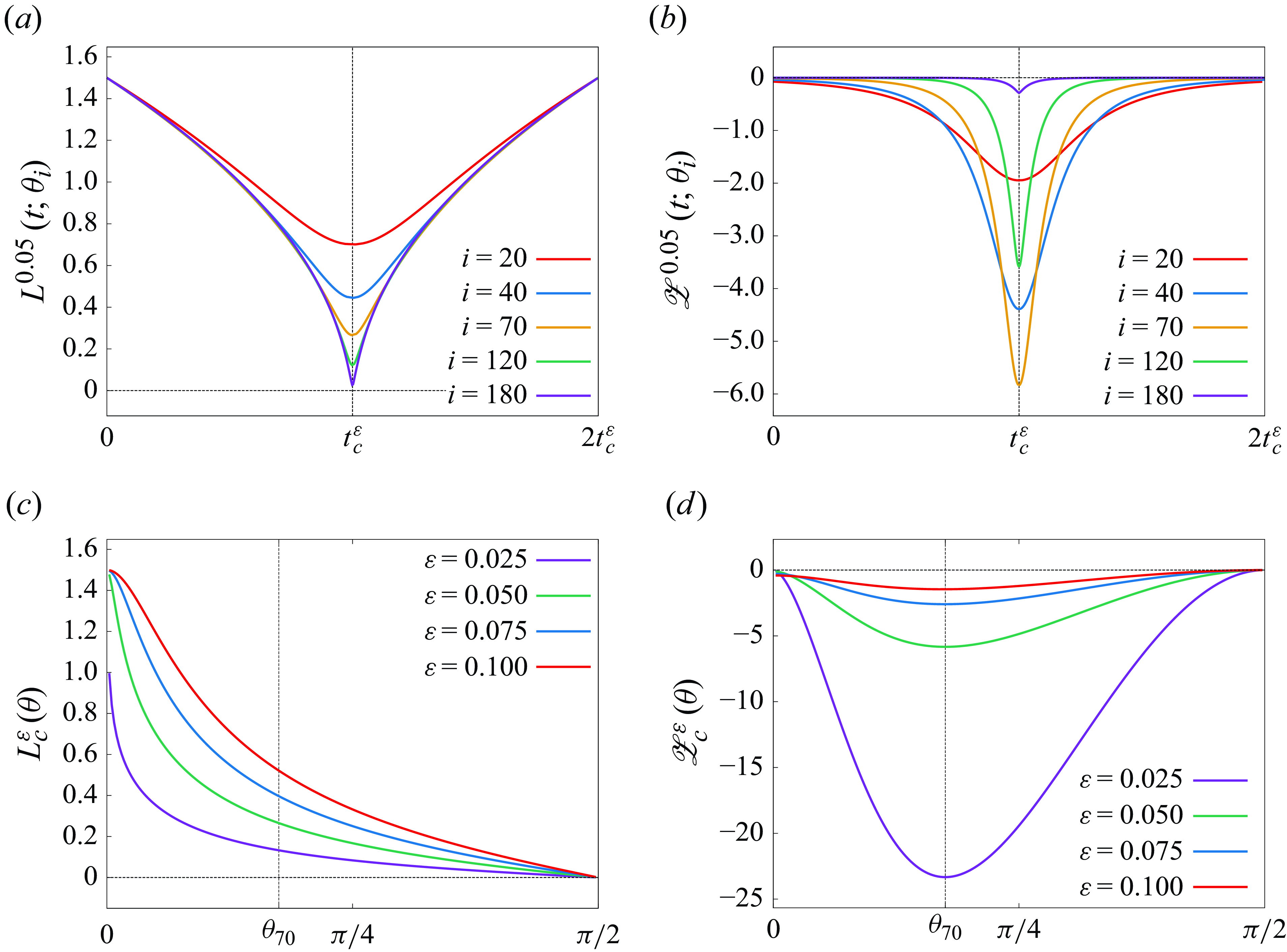
Figure 2. Graphs of (a) $\{ L^{\varepsilon _3}(t; \theta _i) \}_{i \in \mathcal{I}}$ , (b) $\{ {\mathscr{Z}}^{\varepsilon _3}(t;\theta _i) \}_{i \in \mathcal{I}}$ with $\mathcal{I}= \{20, 40, 70, 120, 180 \}$ , (c) $\{ L^{\varepsilon _n}_c(\theta )\}_{n=2}^5$ and (d) $\{ {\mathscr{Z}}^{\varepsilon _n}_c(\theta ) \}_{n=2}^5$ for the three $\alpha$ -PV system. In panels (a) and (b), the time axes are rescaled so that $\{ t_c^\varepsilon (\theta _i) \}_{i \in \mathcal{I}}$ are placed at the same midpoint. The curves in panels (c) and (d) are interpolating data for $i = 1, \ldots {\kern-1pt} , 199$ with lines.

We focus on the total length and the enstrophy at the critical time. As we see in figure 2(c), $L^\varepsilon _c(\theta )$ is monotonically decreasing and, for any fixed $\theta \in (0,\pi /2)$ , it seems to approach zero as $\varepsilon$ gets smaller. Figure 2(d) shows that ${\mathscr{Z}}^\varepsilon _c(\theta )$ has the minimum in $(0,\pi /2)$ and numerical computations suggest

(4.9) \begin{equation} \theta _{69} \lt \operatorname {argmin}_{\theta \in (0,\pi /2)}\, {\mathscr{Z}}^\varepsilon _c(\theta ) \lt \theta _{71} \end{equation}

and $\operatorname {argmin_\theta }\, {\mathscr{Z}}^\varepsilon _c(\theta )$ is independent of $\varepsilon \gt 0$ . We also find from figure 2(d) that, for any fixed $\theta \in (0,\pi /2)$ , ${\mathscr{Z}}^\varepsilon _c(\theta )$ seems to diverge to negative infinity as $\varepsilon$ tends to zero, though it is not a monotonically decreasing function of $\varepsilon$ near $\theta =0$ . Although we omit the figures, numerical computations indicate that the configuration of the three $\alpha$ -point vortices at $t_c^\varepsilon (\theta )$ is a collinear state for any $\varepsilon \gt 0$ and $\theta \in (0,\pi /2)$ , and it is similar to (4.8) with $\theta = 0$ , which is a relative equilibrium of the three-PV system, see § 2.3.

Next, we see the $\varepsilon \to 0$ limits of $L^\varepsilon _c(\theta )$ , ${\mathscr{Z}}^\varepsilon _c(\theta )$ and $t^\varepsilon _c(\theta )$ for $\theta \in (0, \pi /2)$ more precisely. For $i \in \{1,\ldots {\kern-1pt} ,199\}$ , we consider the following three sets of five points on $\mathbb{R}^2$ :

(4.10) \begin{equation} \mathcal{L}(i) := \big\{ (\varepsilon _n^2,L_n(i)) \big\}_{n=1}^5, \quad \mathcal{Z}(i) := \big\{ (\varepsilon _n^2,Z_n(i)) \big\}_{n=1}^5, \quad \mathcal{T}(i) := \big\{ (\varepsilon _n^2,T_n(i))\big\}_{n=1}^5, \end{equation}

where $\{\varepsilon _n \}_{n=1}^5$ is given by (4.7) and $L_n$ , $Z_n$ , $T_n$ are defined by

(4.11) \begin{equation} L_n(i) := \frac {L^{\varepsilon _n}_c(\theta _i)^2}{L^{\varepsilon _5}_c(\theta _i)^2}, \qquad Z_n(i) := \frac {1/ {\mathscr{Z}}^{\varepsilon _n}_c(\theta _i)}{1/|{\mathscr{Z}}^{\varepsilon _5}_c(\theta _i)|} = \frac {|{\mathscr{Z}}^{\varepsilon _5}_c(\theta _i)|}{{\mathscr{Z}}^{\varepsilon _n}_c(\theta _i)}, \qquad T_n(i) := \frac {t^{\varepsilon _n}_c(\theta _i)}{t_c(\theta _i)} - 1. \end{equation}

Here, $t_c(\theta )$ is the collapse time (4.4) in the PV system. Note that we use normalised values of $L^{\varepsilon _n}_c(\theta )$ , $1/{\mathscr{Z}}^{\varepsilon _n}_c(\theta )$ and $t^{\varepsilon _n}_c(\theta )$ divided by $L^{\varepsilon _5}_c(\theta )$ , $1/|{\mathscr{Z}}^{\varepsilon _5}_c(\theta )|$ and $t_c(\theta )$ , respectively. Our purpose is to show that $\mathcal{L}(i)$ , $\mathcal{Z}(i)$ and $\mathcal{T}(i)$ are on curves connected to the origin on ${\mathbb {R}}^2$ for any $i = 1,\ldots {\kern-1pt} ,199$ , which indicates that $L^\varepsilon _c(\theta )$ converges to zero, ${\mathscr{Z}}^\varepsilon _c(\theta )$ diverges to negative infinity and $t^\varepsilon _c(\theta )$ converges to $t_c(\theta )$ in the $\varepsilon \to 0$ limit. We apply the least squares method to $\mathcal{L}(i)$ , $\mathcal{Z}(i)$ and $\mathcal{T}(i)$ , and try to approximate these sets by straight lines. We describe the approximate lines by

(4.12) \begin{equation} y = a_X(i) x + b_X(i), \end{equation}

and the errors between the approximate lines and the three sets by

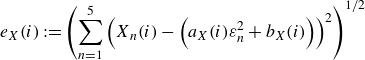(4.13) \begin{equation} e_X(i):= \left ( \sum _{n=1}^5 \left ( X_n(i) - \left ( a_X(i) \varepsilon _n^2 + b_X(i) \right ) \right )^2 \right )^{1/2} \end{equation}

for $X = L, Z, T$ . Figure 3(a) shows the graphs of $b_L(i), b_Z(i), b_T(i)$ and $e_L(i), e_Z(i),$ $e_T(i)$ for $i = 1, \ldots {\kern-1pt} , 199$ . For large $i$ , $\mathcal{L}(i)$ , $\mathcal{Z}(i)$ and $\mathcal{T}(i)$ are well approximated by straight lines connected to the origin since both $(b_L(i), b_Z(i),b_T(i))$ and $(e_L(i), e_Z(i),e_T(i))$ are sufficiently small. Although the errors $e_L(i)$ , $e_Z(i)$ and $e_T(i)$ for small $i$ are large, which means that $\mathcal{L}(i)$ , $\mathcal{Z}(i)$ and $\mathcal{T}(i)$ are not on any straight line, these three sets are still on curves connected to the origin, see figures 3(b), 3(c) and 3(d). Hence, we find from the numerical computations that the desired convergences of $L^\varepsilon _c(\theta )$ , ${\mathscr{Z}}^\varepsilon _c(\theta )$ and $t^\varepsilon _c(\theta )$ hold, and conclude that the enstrophy dissipation occurs by the collapse of three point vortices. We again remark that these numerical results are consistent with the mathematical results of Gotoda & Sakajo (2016b , 2018).

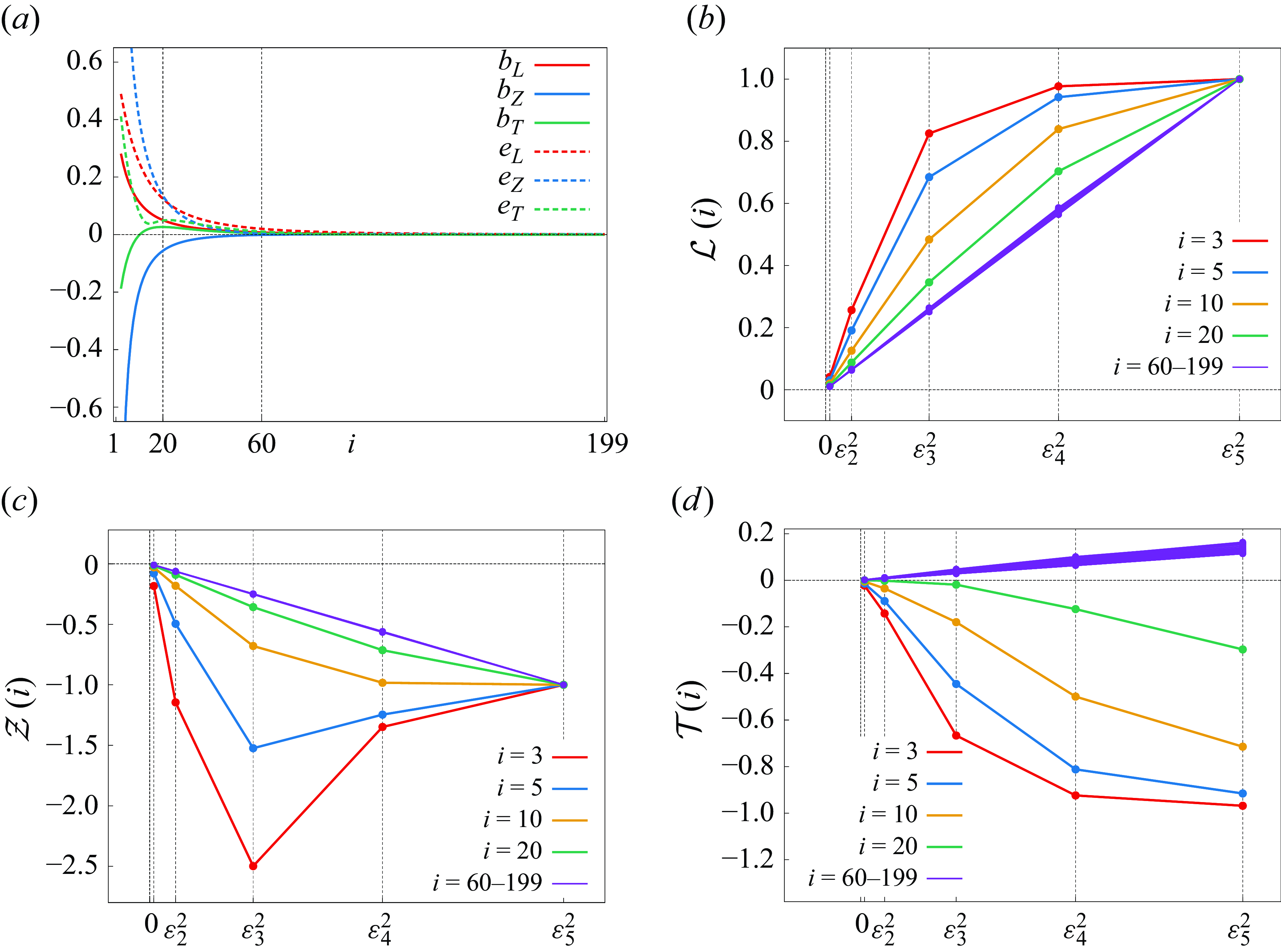
Figure 3. Interpolating curves of (a) $b_L(i), b_Z(i), b_T(i)$ and $e_L(i), e_Z(i), e_T(i)$ , $i = 1, \ldots {\kern-1pt}, 199$ with lines, in which the continuous curves describe $b_L, b_Z, b_T$ and the dashed ones describe $e_L, e_Z, e_T$ . The plots of (b) $\mathcal{L}(i)$ , (c) $\mathcal{Z}(i)$ and (d) $\mathcal{T}(i)$ with interpolating straight lines. The purple graphs in panels (b) and (c) are plotting data for all $i$ from $60$ to $199$ and those in panel (d) are plotting skipped data for $i = j\times 10$ , $j=6,\ldots {\kern-1pt} ,19$ for visibility.

4.3. Four-vortex problem

We consider the four- $\alpha$ -PV system with initial data (2.19) without $k_5$ , that is,

(4.14) \begin{equation} k_1 = \dfrac {1}{2} d_1 e^{i\theta }, \qquad k_2 = - \dfrac {1}{2} d_1 e^{i\theta }, \qquad k_3 = - \dfrac {1}{2} d_2, \qquad k_4 = \dfrac {1}{2} d_2 \end{equation}

for $\theta \in (0, \pi /2)$ . For numerical computations, we set $d_2 = 2$ and $\alpha = -1$ , which determine the other parameters $d_1$ and $\beta$ by the relation $d_1^2 / d_2^2 = - \beta /\alpha = 2 - \sqrt {3}$ .

As we see in figures 4(a) and 4(c), similarly to the three-vortex problem, $L^{\varepsilon _3}(t;\theta _i)$ decreases as time evolves and, after attaining its minimum at $t_c^\varepsilon (\theta _i)$ , it turns to increase, which holds for the other $\varepsilon _n$ as well. At the critical time, $L^{\varepsilon _n}_c(\theta )$ attains its minimum at a certain $\theta _L \in (0, \pi /2)$ and it is monotonically decreasing for $\theta \lt \theta _L$ and increasing for $\theta \gt \theta _L$ , which is a feature different from the three-vortex problem. Numerical computations indicate $\theta _{136} \lt \theta _L \lt \theta _{138}$ for any $\varepsilon _n$ . As $\varepsilon \gt 0$ gets smaller, $L^\varepsilon _c(\theta )$ seems to converge to zero: the four $\alpha$ -point vortices simultaneously collapse at a finite time in the $\varepsilon \to 0$ limit. Regarding the enstrophy, figures 4(b) and 4(d) show that ${\mathscr{Z}}^\varepsilon (t;\theta )$ could be positive for $\theta$ larger than a certain value $\theta _Z \in (0, \pi /2)$ in contrast to the three-vortex problem. More precisely, it is suggested that ${\mathscr{Z}}^\varepsilon (t;\theta )$ is a negative function of $t$ for any fixed $\theta \lt \theta _Z$ , but ${\mathscr{Z}}^\varepsilon (t;\theta )$ for $\theta \gt \theta _Z$ becomes positive around $t_c^\varepsilon (\theta )$ and it is a positive function for sufficiently large $\theta$ . In addition, numerical computations show that, as a function of $t$ , ${\mathscr{Z}}^\varepsilon (t, \theta _i)$ has one local extremum at $t_c^\varepsilon (\theta _i)$ for $i \leqslant 132$ and $i \geqslant 173$ , that is, the value ${\mathscr{Z}}^\varepsilon _c(\theta _i)$ is the global minimum for $i \leqslant 132$ and the global maximum for $\theta \geqslant 173$ . For the case of $132 \lt i \lt 173$ , ${\mathscr{Z}}^\varepsilon (t;\theta _i)$ is in a transition process: the critical time $t_c^\varepsilon (\theta _i)$ is not just one extremum but ${\mathscr{Z}}^\varepsilon (t;\theta _i)$ has several extrema, see figures 5(a) and 5(b). Focusing on the critical time, ${\mathscr{Z}}^\varepsilon _c(\theta )$ attains its minimum around $\theta = \theta _{66}$ and maximum around $\theta = \theta _{160}$ . The sign of ${\mathscr{Z}}^\varepsilon _c(\theta )$ changes at $\theta = \theta _Z$ satisfying $\theta _{137} \lt \theta _Z \lt \theta _{138}$ . Considering the $\varepsilon \to 0$ limit, ${\mathscr{Z}}^\varepsilon _c(\theta )$ seems to diverge to negative infinity for $\theta \lt \theta _Z$ and positive infinity for $\theta \gt \theta _Z$ . Namely, the enstrophy dissipation by collapse of the four $\alpha$ -point vortices in the $\varepsilon \to 0$ limit occurs for $\theta \lt \theta _Z$ . It is numerically suggested that $\theta _Z$ is the same value as $\theta _L$ which we describe by $\theta _c$ , and the critical angle $\theta _c$ is a universal constant with respect to $\varepsilon \gt 0$ .

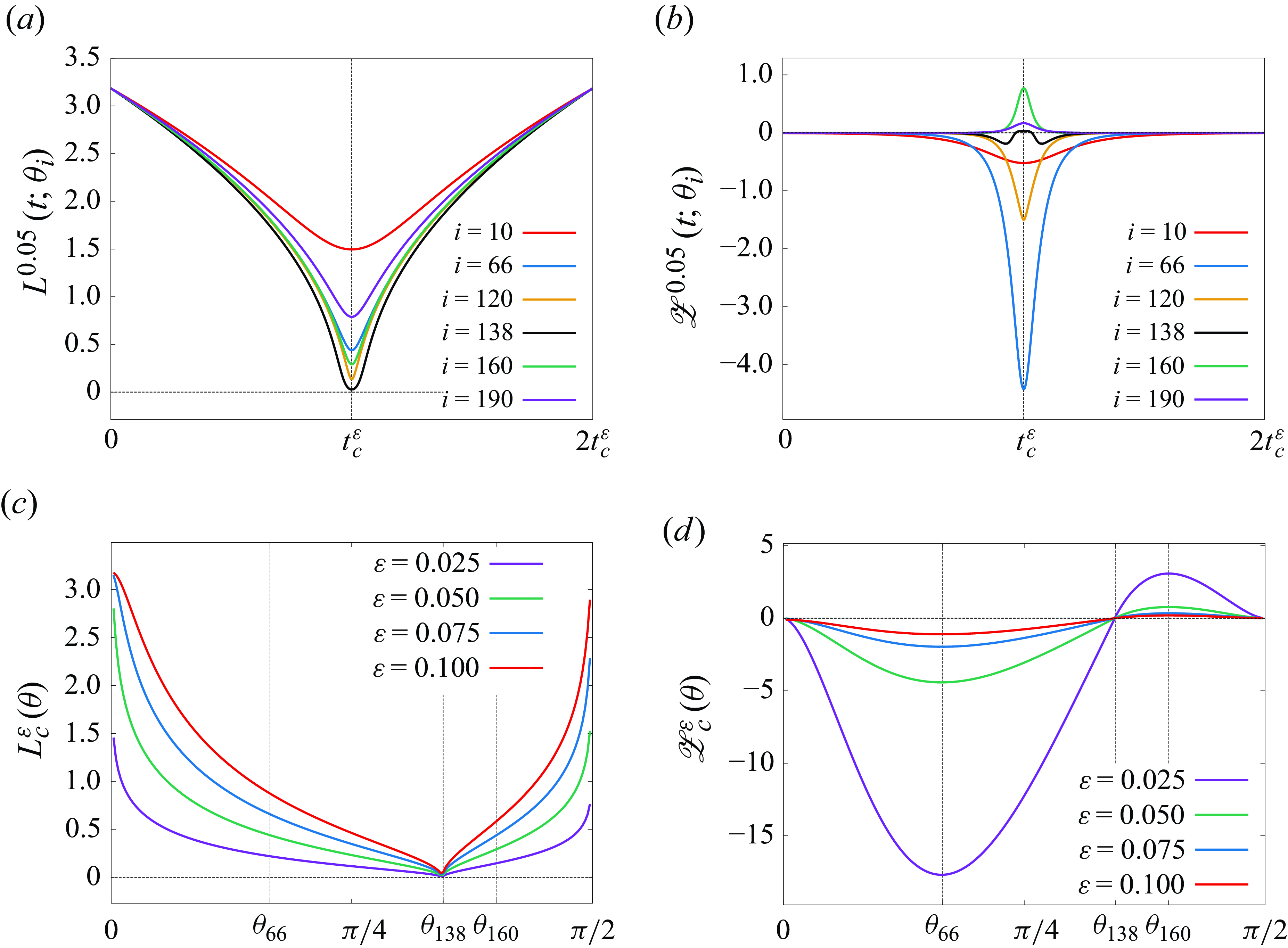
Figure 4. Graphs of (a) $\{ L^{\varepsilon _3}(t; \theta _i) \}_{i \in \mathcal{I}}$ , (b) $\{ {\mathscr{Z}}^{\varepsilon _3}(t;\theta _i) \}_{i \in \mathcal{I}}$ with $\mathcal{I}= \{10, 66, 120, 138, 160, 190 \}$ , (c) $\{ L^{\varepsilon _n}_c(\theta )\}_{n=2}^5$ and (d) $\{ {\mathscr{Z}}^{\varepsilon _n}_c(\theta ) \}_{n=2}^5$ for the four- $\alpha$ -PV system. Similarly to figure 2, the time axes are rescaled in panels (a) and (b), and the graphs of panels (c) and (d) are interpolating curves for $i = 1, \ldots {\kern-1pt} , 199$ .

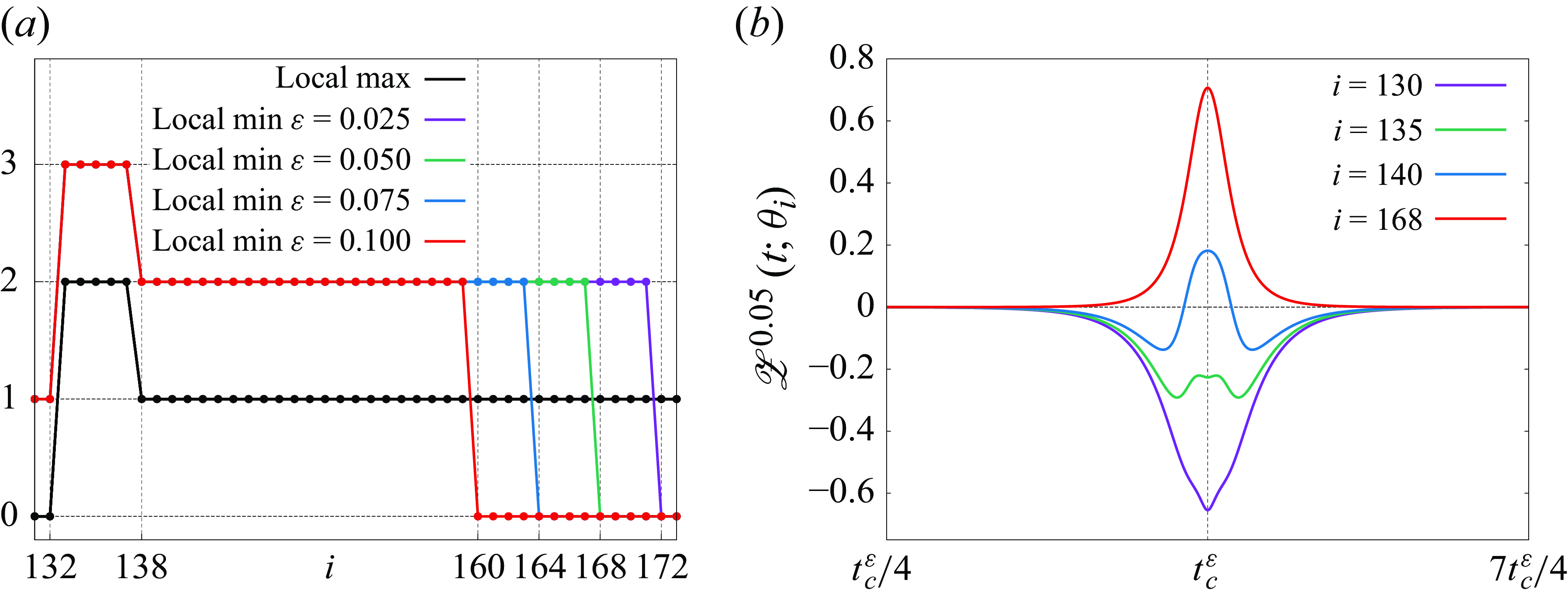
Figure 5. (a) Numbers of local maximum and local minimum of ${\mathscr{Z}}^{\varepsilon }(t;\theta _i)$ for $i =131,\ldots {\kern-1pt} , 173$ . (b) Graphs of $\{ {\mathscr{Z}}^{\varepsilon _3}(t;\theta _i) \}_{i \in \{130,135,140,168 \}}$ .

We remark on the configuration of the four $\alpha$ -point vortices at the critical time. Figure 6(a) shows the rescaled configurations at $t_c^{\varepsilon _3}(\theta _i)$ for $i=1,\ldots {\kern-1pt} ,199$ and figure 6(b) shows the angle between $l^{\varepsilon _3}_{12}(t_c^{\varepsilon _3};\theta _i)$ and $l^{\varepsilon _3}_{34}(t_c^{\varepsilon _3};\theta _i)$ divided by $\pi$ , which is denoted by $\theta _d(i)/\pi$ . For any $i = 1,\ldots {\kern-1pt} ,137$ , the configuration at the critical time is a collinear state whose enstrophy ${\mathscr{Z}}^\varepsilon _c(\theta _i)$ is negative, see figure 4(d). For $i = 138,\ldots {\kern-1pt} ,199$ , the four $\alpha$ -point vortices form a rhombus at $t_c^\varepsilon (\theta _i)$ and ${\mathscr{Z}}^\varepsilon _c(\theta _i)$ has a positive value, which has never been observed in the three-vortex problem. Thus, $\theta _c$ is also critical in terms of the configuration of $\alpha$ -point vortices at the critical time. It is noteworthy that the collinear and the rhombus states observed in figure 6(a) are the same as (4.14) with $\theta = 0$ and $\theta =\pi /2$ , that is, relative equilibria in the four-PV system. We have numerically obtained the same figures as figure 6 for the other $\varepsilon _n$ . Thus, the enstrophy dissipation could occur by vortex collapse in the $\varepsilon \to 0$ limit of the four $\alpha$ -point vortices keeping a collinear configuration.

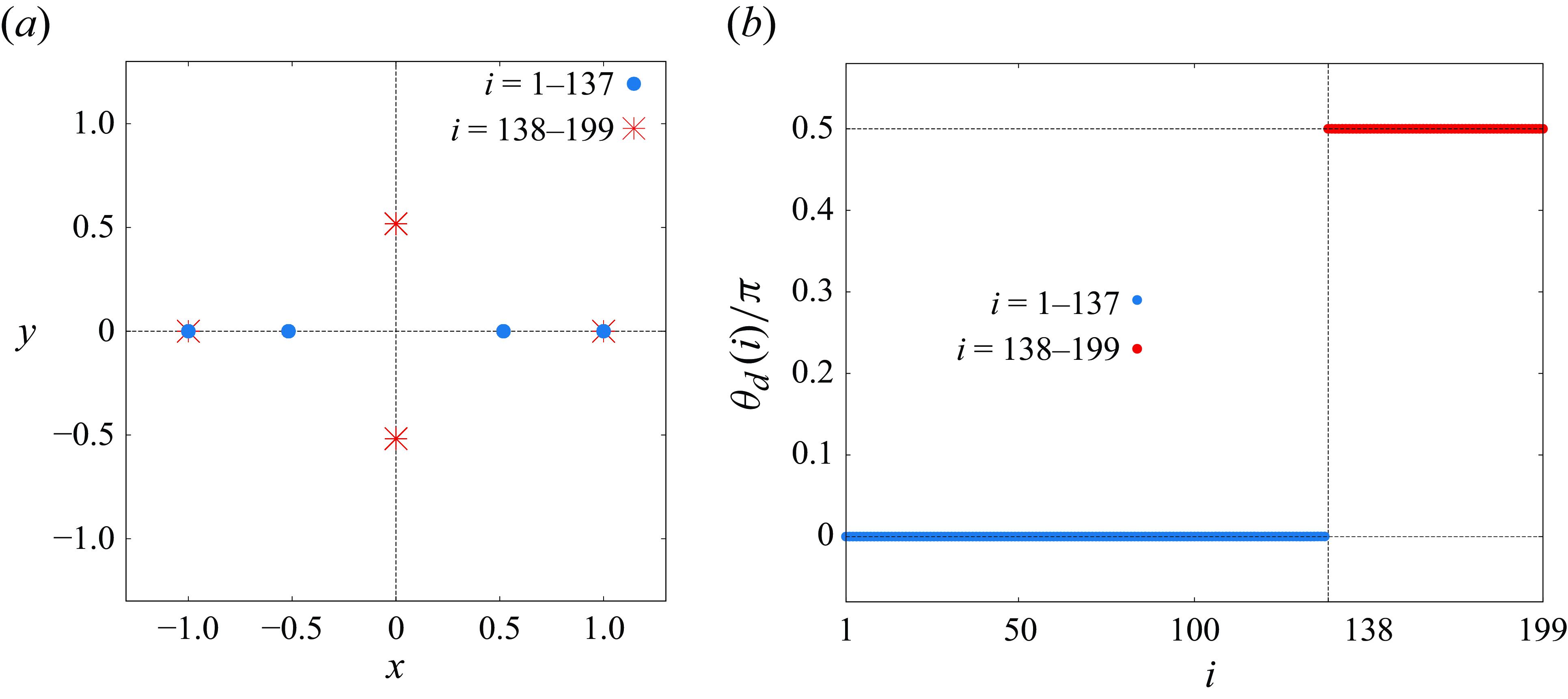
Figure 6. (a) Rescaled configurations of the four $\alpha$ -point vortices at $t_c^{\varepsilon _3}(\theta _i)$ . (b) Angle between the diagonals $l^{\varepsilon _3}_{12}(t_c^{\varepsilon _3};\theta _i)$ and $l^{\varepsilon _3}_{34}(t_c^{\varepsilon _3};\theta _i)$ divided by $\pi$ .

Next, we investigate the $\varepsilon \to 0$ limits of $L^\varepsilon _c(\theta )$ , ${\mathscr{Z}}^\varepsilon _c(\theta )$ and $t^\varepsilon _c(\theta )$ . In the same manner as the three-vortex problem, we consider the three sets $\mathcal{L}(i)$ , $\mathcal{Z}(i)$ and $\mathcal{T}(i)$ in (4.10), and show that $\mathcal{L}(i)$ , $\mathcal{Z}(i)$ and $\mathcal{T}(i)$ are on curves connected to the origin for any $i=1,\ldots {\kern-1pt} ,199$ . We also use the same notation about the approximate lines (4.12) and the errors (4.13) based on the least squares method. Figure 7(a) shows graphs of $b_L(i), b_Z(i), b_T(i)$ and $e_L(i), e_Z(i), e_T(i)$ for $i = 1, \ldots {\kern-1pt}, 199$ . Except for $\theta _i$ near $i =0$ and $i=199$ , the three curves interpolating $\mathcal{L}(i)$ , $\mathcal{Z}(i)$ and $\mathcal{T}(i)$ with lines are approximated by straight lines and the errors $e_L(i)$ , $e_Z(i)$ , $e_T(i)$ are sufficiently small. Note that, for $\theta _i$ around the critical angle $\theta _c$ , absolute values of $b_L(i)$ , $b_Z(i)$ , $e_L(i)$ and $e_Z$ are slightly larger than zero, but they are still well approximated by straight lines. As for $\theta _i$ near $i=0$ and $i=199$ , the errors $e_L(i)$ , $e_Z(i)$ and $e_T(i)$ are large, and thus the three sets are not on any straight line. However, they are on curves connected to the origin, see figures 7(b), 7(c) and 7(d). Hence, numerical computations indicate that, for any $\theta \in (0, \pi /2)$ , the solution to the four- $\alpha$ -PV system with (4.14) converges to a collapsing orbit with the collapse time $t_c(\theta )$ and the enstrophy diverges to infinity: it diverges to negative infinity for $\theta \lt \theta _c$ and positive infinity for $\theta \gt \theta _c$ .

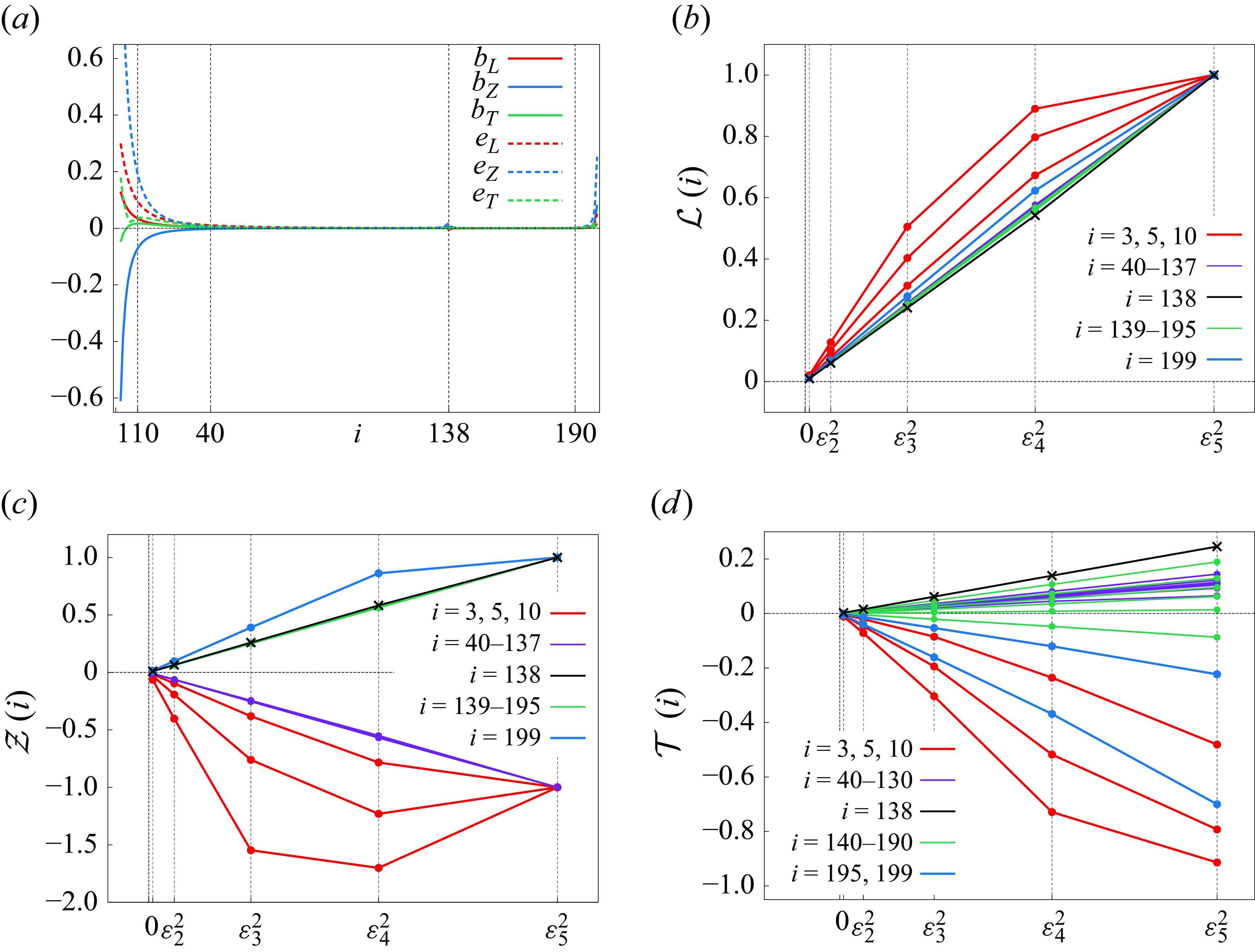
Figure 7. Interpolating curves of (a) $b_L(i), b_Z(i), b_T(i)$ and $e_L(i), e_Z(i), e_T(i)$ , $i = 1, \ldots {\kern-1pt}, 199$ with lines. Plots of (b) $\mathcal{L}(i)$ , (c) $\mathcal{Z}(i)$ and (d) $\mathcal{T}(i)$ with lines. The purple and green graphs in panels (b) and (c) are plotting data for all $i$ in the described ranges and those in panel (d) are plotting skipped data for $i = j\times 10$ , $j=4,\ldots {\kern-1pt} ,19$ .

Finally, we show that the convergences (3.20) and (3.21) in the sense of distributions hold for the four-vortex problem with $\theta \in (0, \theta _c)$ . The abovementioned analysis about the $\varepsilon \to 0$ limit has already shown (3.20) for $\theta \in (0, \pi /2)$ . To see that ${\mathscr{Z}}^\varepsilon$ converges to the Dirac delta function, it is sufficient to show that, for any $\theta \in (0, \theta _c)$ , there exists a constant $m_z(\theta ) \lt 0$ such that

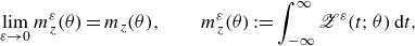(4.15) \begin{equation} \lim _{\varepsilon \to 0} m_z^\varepsilon (\theta ) = m_z(\theta ), \qquad m_z^\varepsilon (\theta ):=\int _{-\infty }^\infty {\mathscr{Z}}^\varepsilon (t; \theta )\, {\textrm d}t, \end{equation}

since we have already confirmed

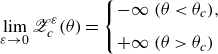(4.16) \begin{equation} \lim _{\varepsilon \to 0} {\mathscr{Z}}^\varepsilon _c(\theta ) = \left \{ \begin{array}{ll} - \infty & (\theta \lt \theta _c), \\[8pt] + \infty & (\theta \gt \theta _c) \end{array} \right . \end{equation}

and

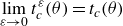(4.17) \begin{equation} \lim _{\varepsilon \to 0} t_c^\varepsilon (\theta ) = t_c(\theta ) \end{equation}

for any $\theta \in (0, \pi /2)$ . As we see in figure 8(a), for any fixed $\theta \in (0, \pi /2)$ , $m_z^\varepsilon (\theta )$ converges to a certain value as $\varepsilon$ tends to zero. Thus, defining the function $m_z(\theta )$ by the pointwise limit, we obtain the convergence to the Dirac delta function. Note that ${\mathscr{Z}}^\varepsilon (t,\theta )$ has several local minima for $\theta \in (\theta _{132}, \theta _c)$ , see figure 5(a), and thus the convergence to the Dirac delta function is not obvious. However, as we see in figure 8(b), the times when ${\mathscr{Z}}^\varepsilon (t,\theta _{137})$ attains its local minima get close to $t_c^\varepsilon (\theta _{137})$ as $\varepsilon$ tends to zero, that is, it converges to the collapse time $t_c(\theta _{137})$ owing to (4.17). Since numerical computations show that the same result holds for $\theta _i$ , $i=133,\ldots {\kern-1pt} ,136$ , we find from (4.16) that the desired convergence holds for any $\theta \in (\theta _{132}, \theta _c)$ . As for the convergence of the energy dissipation rate ${\mathscr{D}}_E^\varepsilon$ , it is enough to show that ${\mathscr{D}}_E^\varepsilon (t-t_c^\varepsilon )$ is an odd and integrable function on $\mathbb R$ , see the proof of theorem 6 of Gotoda & Sakajo (2018). As an example, figure 8(c) shows the graph of ${\mathscr{D}}_E^\varepsilon (t-t_c^\varepsilon ; \theta _{60})$ that is odd and rapidly decreasing as $t$ gets further away from $t_c^\varepsilon (\theta _{60})$ for any $\varepsilon _n$ . Although we omit the figures, numerical computations show that ${\mathscr{D}}_E^\varepsilon (t-t_c^\varepsilon ;\theta _i)$ is odd and integrable for any $i=1, \ldots {\kern-1pt} , 199$ . Thus, we conclude that, for any $\theta \in (0, \theta _c)$ , ${\mathscr{Z}}^\varepsilon (\cdot ; \theta )$ converges to the Dirac delta function with the mass $m_z(\theta ) \lt 0$ and the point support $t= t_c(\theta )$ , and ${\mathscr{D}}_E^\varepsilon (\cdot ;\theta )$ converges to zero in the sense of distributions.

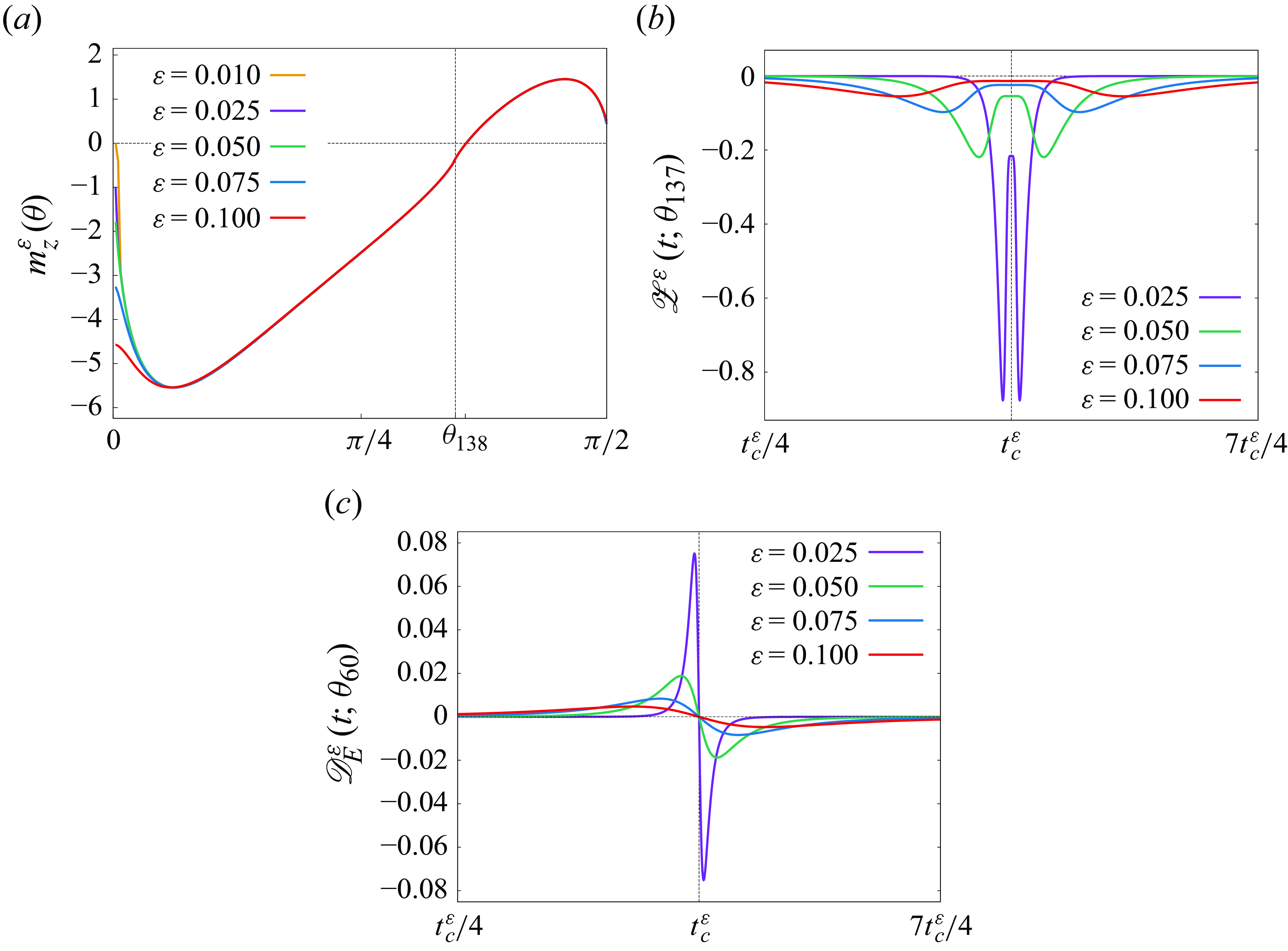
Figure 8. Graphs of (a) $\{ m_z^{\varepsilon _n}(\theta ) \}_{n=1}^5$ , (b) $\{ {\mathscr{Z}}^{\varepsilon }(t,\theta _{137}) \}_{n=2}^5$ and (c) $\{ {\mathscr{D}}_E^{\varepsilon }(t,\theta _{60}) \}_{n=2}^5$ for the four- $\alpha$ -PV system.

4.4. Five-vortex problem

We consider the five-vortex problem with initial data (2.19) for $\theta \in (0,\pi /2)$ . In the following numerical computations, we use the parameters $d_2 = 2$ , $\alpha = -1$ and $\beta = 1/2$ . Then, $d_1$ and $\gamma$ are determined by (2.20).

As we see in figures 9(a) and 9(b), the functions $L^{\varepsilon }(t;\theta _i)$ and ${\mathscr{Z}}^\varepsilon (t;\theta _i)$ behave almost in the same way as the four-vortex problem and numerical computations for the other $\varepsilon _n$ show the same features. As for the values of $L^{\varepsilon }(t;\theta )$ and ${\mathscr{Z}}^\varepsilon (t;\theta )$ at the critical time, figures 9(c) and 9(d) show that there exists a critical angle $\theta _c$ in $(\theta _{83},\theta _{84})$ , which seems to be universal with respect to $\varepsilon \gt 0$ , such that $L^\varepsilon _c(\theta )$ attains its minimum at $\theta = \theta _c$ and ${\mathscr{Z}}^\varepsilon _c(\theta )$ changes its sign before and after $\theta _c$ . In addition, ${\mathscr{Z}}^\varepsilon _c(\theta )$ has the global minimum around $\theta _{41}$ and the global maximum around $\theta _{123}$ . These features are similar to the four-vortex problem, but the critical angle $\theta _c$ for the present parameters $(\alpha , \beta , \gamma )$ is smaller than that observed in the four-vortex problem.

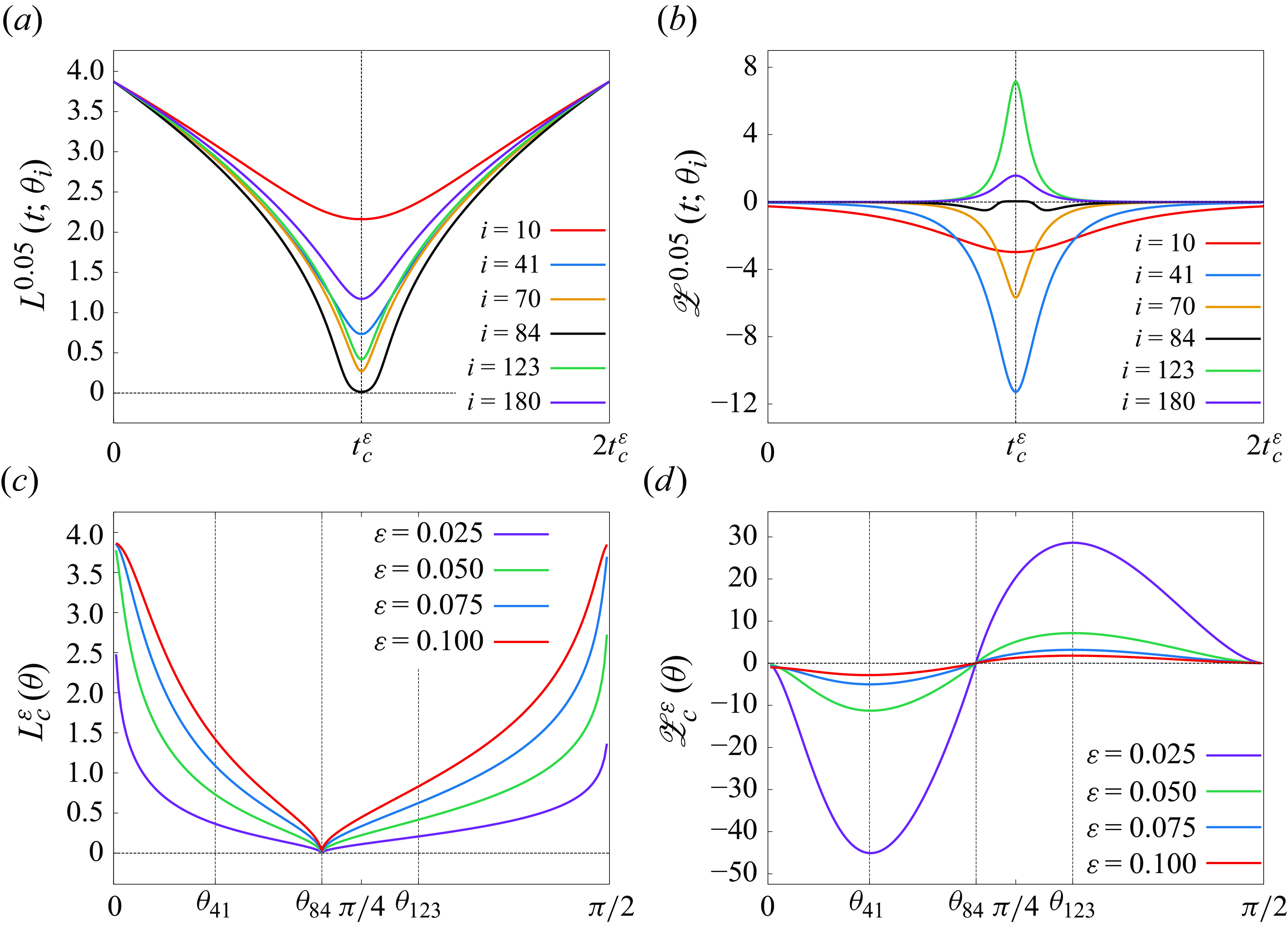
Figure 9. Graphs of (a) $\{ L^{\varepsilon _3}(t; \theta _i) \}_{i \in \mathcal{I}}$ , (b) $\{ {\mathscr{Z}}^{\varepsilon _3}(t;\theta _i) \}_{i \in \mathcal{I}}$ with $\mathcal{I}= \{10, 41, 70, 84, 123, 180 \}$ , (c) $\{ L^{\varepsilon _n}_c(\theta )\}_{n=2}^5$ and (d) $\{ {\mathscr{Z}}^{\varepsilon _n}_c(\theta ) \}_{n=2}^5$ for the five- $\alpha$ -PV system. Similarly to figures 2 and 4, the time axes are rescaled in panels (a) and (b), and the graphs of panels (c) and (d) are interpolating curves for $i = 1, \ldots {\kern-1pt} , 199$ .

As for the behaviour of ${\mathscr{Z}}^\varepsilon (t, \theta _i)$ for $\theta _i$ around $\theta _c$ , similarly to the four-vortex problem, the number of its extremum is not single and there is a transition process, see figure 10 for the details. The configuration of the five $\alpha$ -point vortices at the critical time also varies before and after $\theta _c$ : configurations for $\theta \lt \theta _c$ are collinear states and those for $\theta \gt \theta _c$ are rhombuses, see figure 11. Note that the abovementioned collinear and rhombus states are similar to relative equilibria (2.19) with $\theta = 0$ and $\theta =\pi /2$ in the five-PV system. Since we have obtained the same result as figure 11 for the other $\varepsilon _n$ , the enstrophy dissipation is caused by the collapse in the $\varepsilon \to 0$ limit of the five $\alpha$ -point vortices keeping a collinear configuration as well as the four-vortex problem.

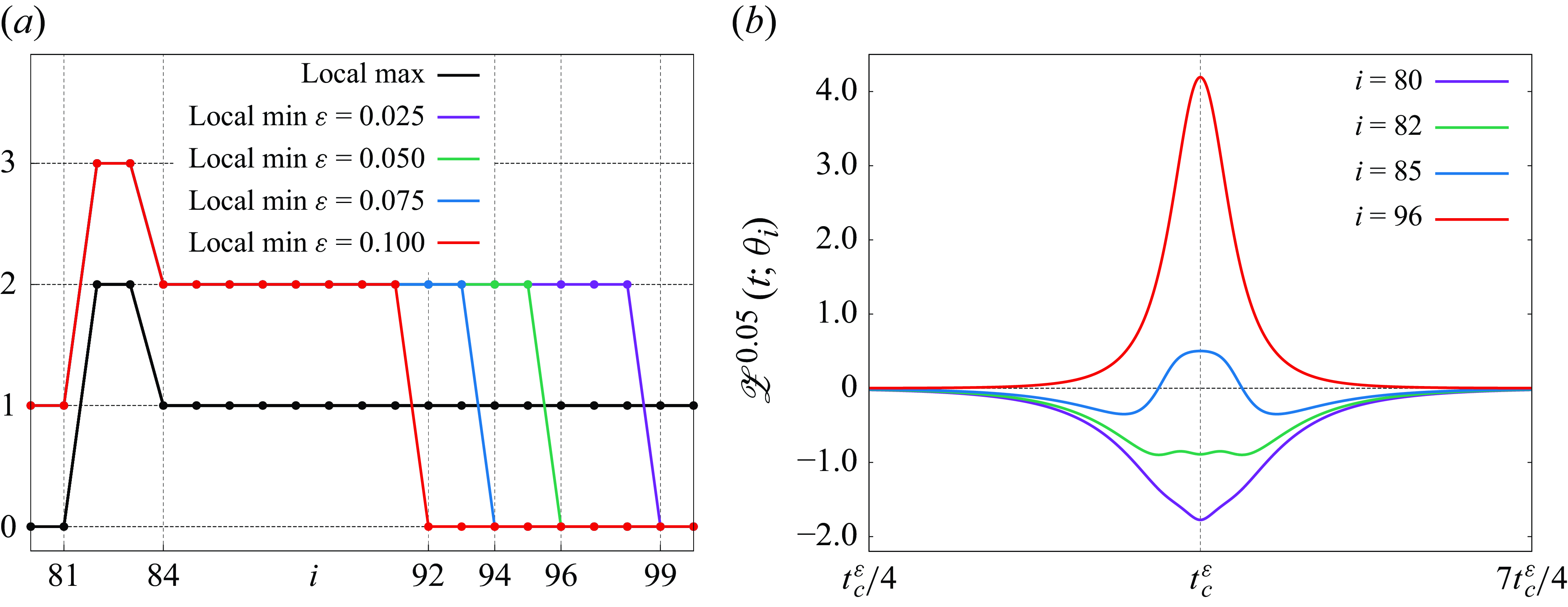
Figure 10. (a) Numbers of local maximum and local minimum of ${\mathscr{Z}}^{\varepsilon }(t;\theta _i)$ for $i =80,\ldots {\kern-1pt} , 100$ . (b) Graphs of $\{ {\mathscr{Z}}^{\varepsilon _3}(t;\theta _i) \}_{i \in \{80,82,85,96 \}}$ .

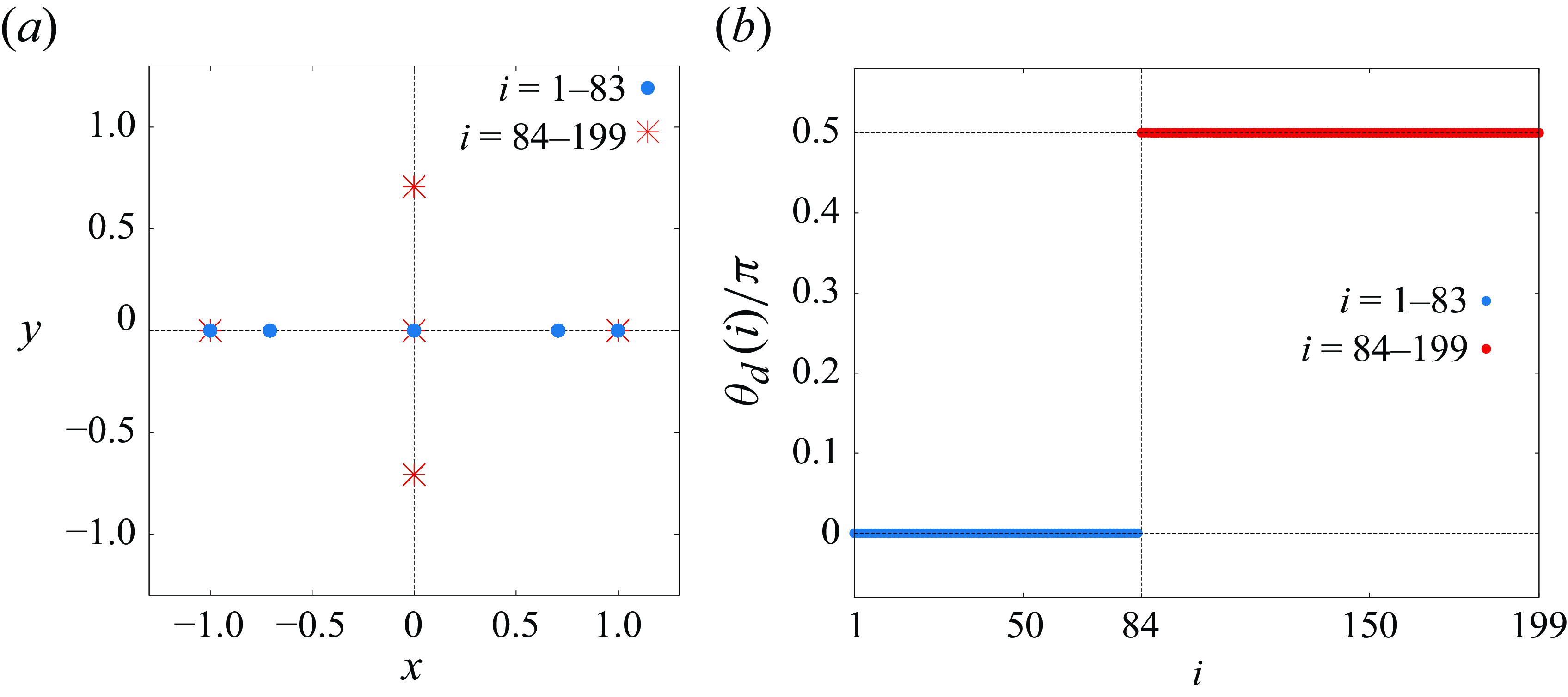
Figure 11. (a) Rescaled configurations of the five $\alpha$ -point vortices at $t_c^{\varepsilon _3}(\theta _i)$ . (b) Angle between the diagonals $l^{\varepsilon _3}_{12}(t_c^{\varepsilon _3};\theta _i)$ and $l^{\varepsilon _3}_{34}(t_c^{\varepsilon _3};\theta _i)$ divided by $\pi$ .

We investigate the $\varepsilon \to 0$ limits of $L^\varepsilon _c(\theta )$ , ${\mathscr{Z}}^\varepsilon _c(\theta )$ and $t^\varepsilon _c(\theta )$ by considering $\mathcal{L}(i)$ , $\mathcal{Z}(i)$ and $\mathcal{T}(i)$ in (4.10) and using the notation (4.12) and (4.13) based on the least squares method. As we see in figure 12(a), except for $\theta _i$ near $i =0$ , $i=84$ and $i=199$ , the three curves interpolating $\mathcal{L}(i)$ , $\mathcal{Z}(i)$ and $\mathcal{T}(i)$ are approximated by straight lines and $b_L(i)$ , $b_Z(i)$ , $b_T(i)$ are sufficiently close to zero. Although the errors $e_L(i)$ , $e_Z(i)$ and $e_T(i)$ near $i =0$ , $i =84$ and $i=199$ are large and their data are not on any straight line, they are on curves connected to the origin, see figures 12(b), 12(c) and 12(d). Thus, we conclude that, for any $\theta \in (0, \pi /2)$ , the solution to the five- $\alpha$ -PV system with (2.19) converges to a collapsing orbit with the collapse time $t_c(\theta )$ , which is equivalent to (3.20), and the enstrophy diverges to negative infinity for $\theta \lt \theta _c$ and positive infinity for $\theta \gt \theta _c$ .

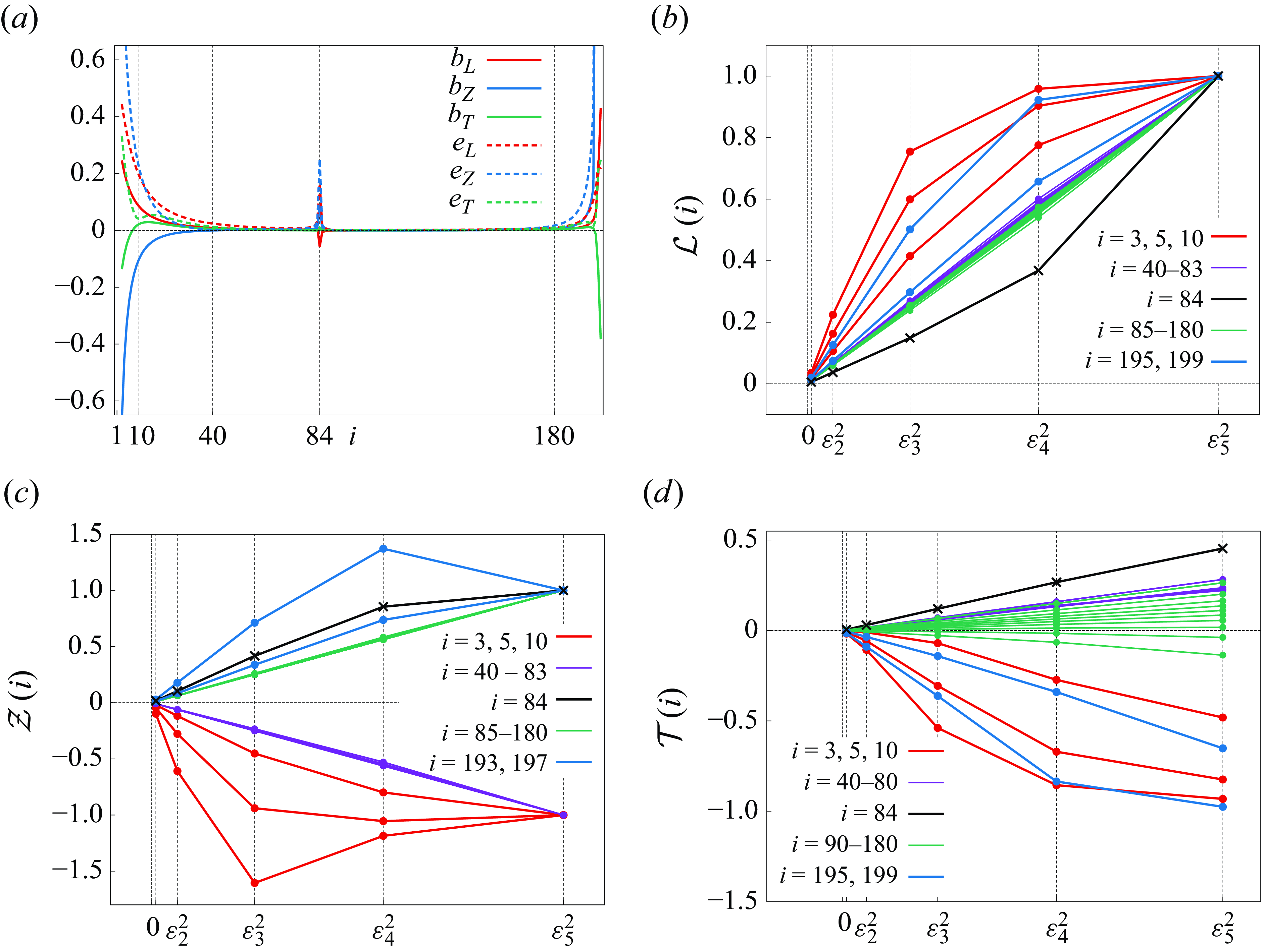
Figure 12. Interpolating curves of (a) $b_L(i), b_Z(i), b_T(i)$ and $e_L(i), e_Z(i), e_T(i)$ , $i = 1, \ldots {\kern-1pt}, 199$ with lines. The plots of (b) $\mathcal{L}(i)$ , (c) $\mathcal{Z}(i)$ and (d) $\mathcal{T}(i)$ with lines. The purple and green graphs in panels (b) and (c) are plotting data for all $i$ in the described range and those in panel (d) are plotting skipped data for $i = j\times 10$ , $j=4,\ldots {\kern-1pt} ,18$ .

As for the convergence (3.21), figure 13(a) shows that, for any fixed $\theta \in (0, \pi /2)$ , $m_z^\varepsilon (\theta )$ converges to a constant in the $\varepsilon \to 0$ limit. Thus, similarly to the four-vortex problem, we define the function $m_z(\theta )$ by the pointwise limit and then find

(4.18) \begin{equation} \lim _{\varepsilon \to 0} m_z^\varepsilon (\theta ) = m_z(\theta ) \end{equation}

for $\theta \in (0, \pi /2)$ and, especially, $m_z(\theta ) \lt 0$ for $\theta \in (0,\theta _c)$ . Since (4.16) follows from the abovementioned argument about the $\varepsilon \to 0$ limit, we obtain the convergence (3.21). Although figure 10(a) shows that ${\mathscr{Z}}^\varepsilon (t,\theta )$ has several local minima for any $\theta \in (\theta _{81}, \theta _c)$ , we find from figure 13(b) that the convergence of ${\mathscr{Z}}^\varepsilon (t,\theta )$ to the Dirac delta function still holds in the same manner as the four-vortex problem. As for ${\mathscr{D}}_E^\varepsilon$ , figure 13(c) and other numerical computations indicate that ${\mathscr{D}}_E^{\varepsilon }(t-t_c^\varepsilon ; \theta _{60})$ is an odd and integrable function for any $\varepsilon \gt 0$ , and ${\mathscr{D}}_E^{\varepsilon }(t-t_c^\varepsilon ; \theta _i)$ is as well for $i=1, \ldots {\kern-1pt} , 199$ . Thus, we conclude that, for any $\theta \in (0, \theta _c)$ , ${\mathscr{Z}}^\varepsilon (\cdot ; \theta )$ converges to the Dirac delta function with the negative mass $m_z(\theta ) \lt 0$ and the support $t= t_c(\theta )$ , and ${\mathscr{D}}_E^\varepsilon (\cdot ;\theta )$ converges to zero in the sense of distributions.

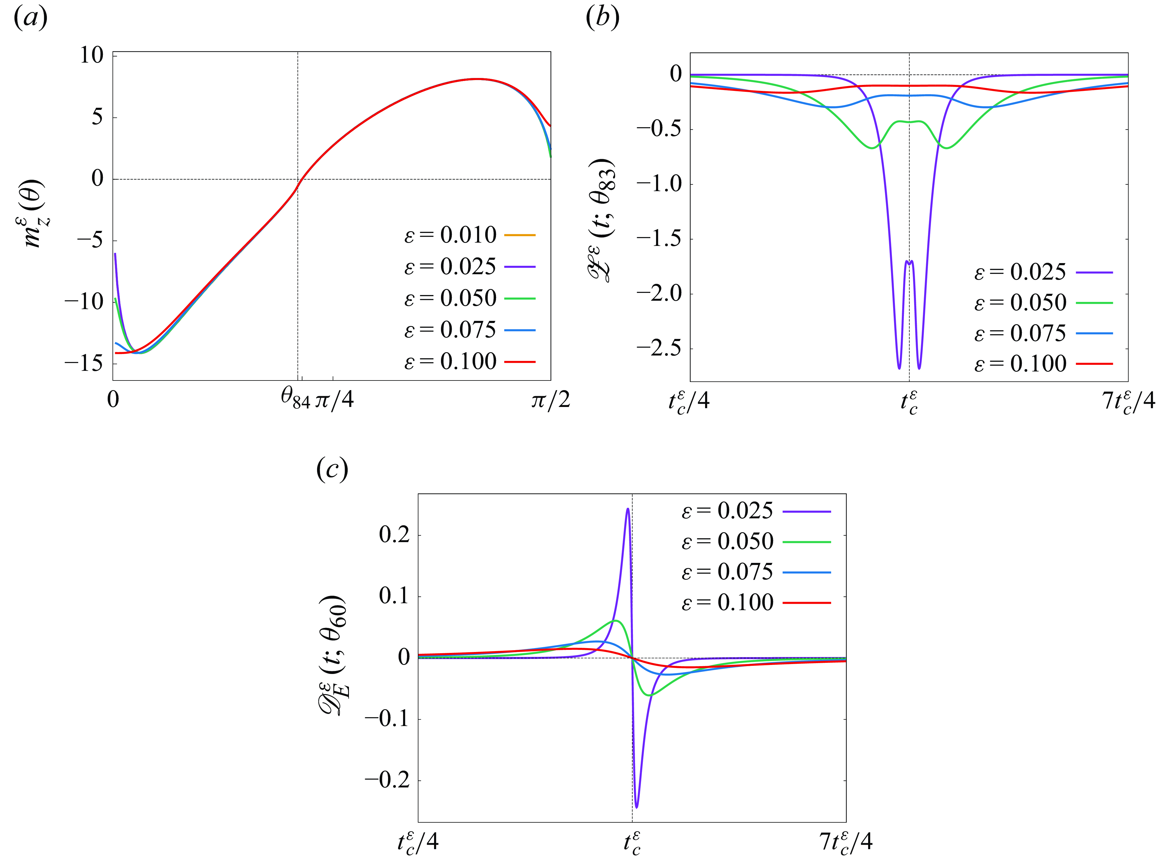
Figure 13. Graphs of (a) $\{ m_z^{\varepsilon _n}(\theta ) \}_{n=1}^5$ , (b) $\{ {\mathscr{Z}}^{\varepsilon }(t,\theta _{83}) \}_{n=2}^5$ and (c) $\{ {\mathscr{D}}_E^{\varepsilon }(t,\theta _{60}) \}_{n=2}^5$ for the five- $\alpha$ -PV system.

4.5. Remark on the total enstrophy and the Hamiltonian energy

Recall that the total enstrophy (3.12) consists of the constant term and the time-dependent term, that is,

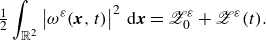(4.19) \begin{equation} \tfrac {1}{2}\int _{\mathbb{R}^2} \left \vert \omega ^\varepsilon ({\boldsymbol x}, t) \right \vert ^2 \,{\textrm d}{\boldsymbol x} = {\mathscr{Z}}^\varepsilon _0 + {\mathscr{Z}}^\varepsilon (t). \end{equation}

In the Euler- $\alpha$ model, it follows from $2 \pi \widehat {h}(s) = (1 + s^2)^{-1}$ that

(4.20) \begin{equation} {\mathscr{Z}}^\varepsilon _0 = \frac {1}{8 \pi \varepsilon ^2} \sum _{m=1}^N \Gamma _m^2, \quad {\mathscr{Z}}^\varepsilon (t;\theta ) = \frac {1}{4\pi \varepsilon ^2} \sum _{m=1}^N \sum _{n=m+1}^N \Gamma _m \Gamma _n \frac {l_{mn}^\varepsilon (t;\theta )}{\varepsilon } K_1 \left ( \frac {l_{mn}^\varepsilon (t;\theta )}{\varepsilon } \right ). \end{equation}

We now show that the total enstrophy diverges to positive infinity in the $\varepsilon \to 0$ limit for any $\theta \in (0,\pi /2)$ . For the case of $t \neq t_c(\theta )$ in (4.4), Gotoda (2020) has proven that the solution to the FPV system converges to the solution to the PV system with the same initial data, that is,

(4.21) \begin{equation} \lim _{\varepsilon \to 0} l_{mn}^\varepsilon (t;\theta ) = l_{mn}(t;\theta ) \gt 0, \qquad t \neq t_c(\theta ), \end{equation}

where $l_{mn}(t;\theta )$ is the mutual distance of the $m$ th and $n$ th point vortices in the PV system. Thus, considering $K_1(r) \sim e^{-r}$ as $r \to \infty$ , we find that ${\mathscr{Z}}^\varepsilon (t;\theta )$ converges to zero as $\varepsilon \to 0$ for any $\theta \in (0,\pi /2)$ , and the total enstrophy diverges to positive infinity due to the divergence of ${\mathscr{Z}}^\varepsilon _0$ . For the case of $t = t_c(\theta )$ , as we see in § 4, it has been shown that

(4.22) \begin{equation} \lim _{\varepsilon \to 0} l_{mn}^\varepsilon \big(t_c^\varepsilon (\theta );\theta \big) = 0, \qquad \lim _{\varepsilon \to 0} t_c^\varepsilon (\theta ) = t_c(\theta ) \end{equation}

and the divergence of ${\mathscr{Z}}^\varepsilon _c (\theta )$ for $\theta \neq \theta _c$ in the $\varepsilon \to 0$ limit. We consider

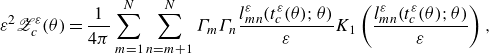(4.23) \begin{equation} \varepsilon ^2 {\mathscr{Z}}^\varepsilon _c(\theta ) = \frac {1}{4\pi } \sum _{m=1}^N \sum _{n=m+1}^N \Gamma _m \Gamma _n \frac {l_{mn}^\varepsilon \big(t_c^\varepsilon (\theta ); \theta \big)}{\varepsilon } K_1 \left ( \frac {l_{mn}^\varepsilon \big(t_c^\varepsilon (\theta );\theta \big)}{\varepsilon } \right ), \end{equation}

and plot the data set

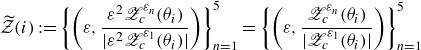(4.24) \begin{equation} \widetilde {\mathcal{Z}}(i) :=\left \{ \left (\varepsilon , \frac {\varepsilon ^2{\mathscr{Z}}^{\varepsilon _n}_c(\theta _i)}{|\varepsilon ^2 {\mathscr{Z}}^{\varepsilon _1}_c(\theta _i)|} \right ) \right \}_{n=1}^5 = \left \{ \left (\varepsilon , \frac {{\mathscr{Z}}^{\varepsilon _n}_c(\theta _i)}{|{\mathscr{Z}}^{\varepsilon _1}_c(\theta _i)|} \right ) \right \}_{n=1}^5 \end{equation}

on $\mathbb{R}^2$ for $i=1,\ldots {\kern-1pt} ,199$ in figure 14. Then, we find from the figures that $\varepsilon ^2 {\mathscr{Z}}^\varepsilon _c(\theta )$ converges to a non-zero constant as $\varepsilon \to 0$ and the limit value is quite close to $\varepsilon _1^2 {\mathscr{Z}}^{\varepsilon _1}_c(\theta )$ . Hence, both ${\mathscr{Z}}^\varepsilon _0$ and ${\mathscr{Z}}^\varepsilon _c(\theta )$ diverge with the same order $1/\varepsilon ^2$ and it is enough to compare the values of $\varepsilon ^2{\mathscr{Z}}^\varepsilon _0$ , which no longer depends on $\varepsilon$ , and $\varepsilon _1^2{\mathscr{Z}}^{\varepsilon _1}_c(\theta )$ to show the divergence of the total enstrophy. The value of $\varepsilon ^2{\mathscr{Z}}^\varepsilon _0$ and the range of $\varepsilon _1^2{\mathscr{Z}}^{\varepsilon _1}_c(\theta )$ obtained by numerical computations are as follows:

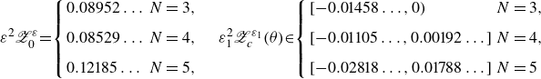(4.25) \begin{equation} \varepsilon ^2 {\mathscr{Z}}^\varepsilon _0\! =\! \left \{ \begin{array}{ll} 0.08952\ldots {\kern-1pt} & N=3, \\[8pt] 0.08529\ldots {\kern-1pt} & N=4, \\[8pt] 0.12185\ldots {\kern-1pt} & N=5, \end{array} \right . \quad \varepsilon _1^2 {\mathscr{Z}}^{\varepsilon _1}_c(\theta ) \!\in \! \left \{ \begin{array}{ll} \lbrack -0.01458\ldots {\kern-1pt} , 0) & N=3, \\[8pt] \lbrack -0.01105\ldots {\kern-1pt} , 0.00192\ldots {\kern-1pt} \rbrack & N=4, \\[8pt] \lbrack -0.02818\ldots {\kern-1pt} , 0.01788\ldots {\kern-1pt} \rbrack & N=5 \end{array} \right . \end{equation}

for any $\theta \in (0, \pi /2)$ . Thus, we conclude that the total enstrophy diverges to positive infinity since

(4.26) \begin{equation} \lim _{\varepsilon \to 0} \left ( \varepsilon ^2{\mathscr{Z}}^\varepsilon _0 + \varepsilon ^2{\mathscr{Z}}^\varepsilon _c(\theta ) \right ) \gt 0 \end{equation}

holds for any $\theta \in (0, \pi /2)$ , that is, the enstrophy produced by self-interaction is relatively larger than the variable enstrophy by mutual interaction of point vortices.

Figure 14. Interpolating curves of $\widetilde {\mathcal{Z}}(i)$ , $i=1,\ldots {\kern-1pt} ,199$ with lines for the (a) four- and (b) five-vortex problems. Three horizontal lines describe $y=1$ , $y=0$ and $y=-1$ .

Next, we see the relation between the enstrophy and the Hamiltonian energy. The numerical computations for the four- and five-vortex problems indicate that the sign of ${\mathscr{Z}}^\varepsilon _c(\theta )$ changes before and after the critical angle $\theta _c$ . We deduce the value of $\theta _c$ in terms of the Hamiltonian energy. Figure 15 shows the graphs of the Hamiltonian energies, $\{{\mathscr{H}}^{\varepsilon _n}(\theta )\}_{n=1}^5$ of the $\alpha$ -PV system with the initial data (2.19) and ${\mathscr{H}}^{{pv}}(\theta )$ in (2.21) of the PV system. We find from the figures that $\{{\mathscr{H}}^{\varepsilon _n}(\theta )\}_{n=1}^5$ and ${\mathscr{H}}^{{pv}}(\theta )$ seem to be zero at $\theta = \theta _c$ and thus we expect that the critical angle $\theta _c$ is the zero point of ${\mathscr{H}}^{{pv}}(\theta )$ . Recall that ${\mathscr{H}}^{{pv}}(\theta )$ is given by

(4.27) \begin{equation} {\mathscr{H}}^{{pv}}(\theta ) = \dfrac {-1}{2 \pi } \log {\left [ c_H d_1^{\alpha (\alpha + 2 \gamma )} d_2^{\beta (\beta + 2 \gamma )} \left (d_1^4 + d_2^4 - 2 d_1^2 d_2^2 \cos {2 \theta } \right )^{\alpha \beta } \right ]}, \end{equation}

Figure 15. Hamiltonian energies ${\mathscr{H}}_{\textrm{pv}}(\theta )$ and ${\mathscr{H}}^\varepsilon (\theta )$ for the (a) four- and (b) five-vortex problems.

where $c_H := 2^{ -4 \alpha \beta - 2 \gamma (\alpha + \beta )}$ , and ${\mathscr{H}}^{{pv}}(\theta )$ is monotonically increasing in $[0,\pi /2]$ . Then, for the four-vortex problem, it is confirmed that ${\mathscr{H}}^{{pv}}(\theta ) \leqslant 0$ is equivalent to

(4.28) \begin{equation} \cos ^2{\theta } \geqslant \frac {3}{2} - 4 (2 - \sqrt {3})^{\sqrt {3}/2} \in (0,1). \end{equation}

Thus, setting

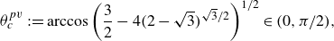(4.29) \begin{equation} \theta _c^{{pv}} := \arccos {\left ( \frac {3}{2} - 4 (2 - \sqrt {3})^{\sqrt {3}/2}\right )^{1/2}} \in (0, \pi /2), \end{equation}

we find ${\mathscr{H}}^{{pv}}(\theta _c^{{pv}}) = 0$ and ${\mathscr{H}}^{{pv}}(\theta ) \lt 0$ for $\theta \lt \theta _c^{{pv}}$ . Note that $\theta _c^{{pv}}$ is independent of the vortex strength $(\alpha , \beta )$ satisfying $-\beta /\alpha = 2 \pm \sqrt {3}$ . For the five-vortex problem, we find that ${\mathscr{H}}^{{pv}}(\theta ) \leqslant 0$ leads to

(4.30) \begin{equation} \cos ^2{\theta } \geqslant F\left (- \frac {\beta }{\alpha } \right ), \quad F(r) := \frac {1}{2} + \frac {1}{4} \left ( r + \frac {1}{r} - 2^{r + 1/r} r^{-1/2 + 1/(1 - r)}\right ). \end{equation}

The function $F(r)$ , $r \gt 0$ satisfies $F(r) = F(1/r)$ , $F(r) \lt 1$ for $r \in (0,\infty )$ and $F(r) \to -\infty$ as $r \to 0+$ and $r \to +\infty$ : there exists $r_0 \in (0,1)$ such that $F(r_0) = F(1/r_0) = 0$ , $F(r) \gt 0$ for $r \in (r_0, 1/r_0)$ and $F(r) \lt 0$ for $r \in (0,r_0)\cup (1/r_0,\infty )$ . Thus, for the vortex strength $(\alpha , \beta )$ satisfying $r_0 \lt -\beta /\alpha \lt 1/r_0$ , the zero point of ${\mathscr{H}}^{{pv}}(\theta )$ is given by

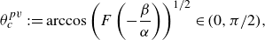(4.31) \begin{equation} \theta _c^{{pv}} := \arccos {\left ( F\left (- \frac {\beta }{\alpha } \right ) \right )^{1/2}} \in (0, \pi /2), \end{equation}

and, for the case of $ - \beta /\alpha \not \in (r_0,1/r_0)$ , ${\mathscr{H}}^{{pv}}(\theta )$ is negative for any $\theta \in (0, \pi /2)$ . Solving $F(r) = 0$ numerically, we obtain $r_0 = 0.24427\ldots {\kern-1pt}$ and $1/r_0 = 4.09373\ldots {\kern-1pt}$ . As the example, the parameters $(\alpha , \beta ) = (-1,1/2)$ used in § 4.4 yield $ - \beta /\alpha = 0.5 \gt 1/r_0$ and

(4.32) \begin{equation} \cos {\theta _c^{{pv}}} = \sqrt {10}/4, \qquad \theta _c^{{pv}} = 0.65905\ldots {\kern-1pt} . \end{equation}

For the angles $\theta _c^{{pv}}$ in (4.29) and (4.32), ${\mathscr{H}}^{\varepsilon }(\theta _c^{{pv}})$ has the following values with 50 decimal digit precision:

(4.33) \begin{align} {\mathscr{H}}^{\varepsilon _1}(\theta _c^{{pv}}) &= 0.00000000000000000000000000000000000000004774156710, \end{align}

(4.34) \begin{align} {\mathscr{H}}^{\varepsilon _2}(\theta _c^{{pv}}) &= 0.00000000000000000796175871454158934707611832596294, \end{align}

(4.35) \begin{align} {\mathscr{H}}^{\varepsilon _3}(\theta _c^{{pv}}) &= 0.00000000048910839350430301244288127565540176406427, \end{align}

(4.36) \begin{align} {\mathscr{H}}^{\varepsilon _4}(\theta _c^{{pv}}) &= 0.00000018223482101614445263682135598596595421823532, \end{align}

(4.37) \begin{align} {\mathscr{H}}^{\varepsilon _5}(\theta _c^{{pv}}) &= 0.00000325269532525068849213275840879218226860975190 \end{align}

for the four vortex problem, and

(4.38) \begin{align} {\mathscr{H}}^{\varepsilon _1}(\theta _c^{{pv}}) &= 0.00000000000000000000000000003652118959255022897325, \end{align}

(4.39) \begin{align} {\mathscr{H}}^{\varepsilon _2}(\theta _c^{{pv}}) &= 0.00000000000070340760920868777298657288061992813740, \end{align}

(4.40) \begin{align} {\mathscr{H}}^{\varepsilon _3}(\theta _c^{{pv}}) &= 0.00000018385254207161893676571683279896647647117553, \end{align}

(4.41) \begin{align} {\mathscr{H}}^{\varepsilon _4}(\theta _c^{{pv}}) &= 0.00001039320650198493256045089710397484679028994850, \end{align}

(4.42) \begin{align} {\mathscr{H}}^{\varepsilon _5}(\theta _c^{{pv}}) &= 0.00007106778013595361344004641215888167270122817411 \end{align}

for the five-vortex problem. Hence, the critical angle $\theta _c$ slightly depends on $\varepsilon \gt 0$ , that is, $\theta _c(\varepsilon )$ , but it converges to $\theta _c^{{pv}}$ rapidly, which insists that $\theta _c^{{pv}}$ is the critical angle for the sign of the enstrophy variation. Finally, we remark on the case of $-\beta /\alpha \not \in (r_0,1/r_0)$ . Figure 16 shows ${\mathscr{H}}^{\varepsilon _3}(\theta )$ and ${\mathscr{Z}}^{\varepsilon _3}_c(\theta )$ for $\alpha = -2.05$ , $\beta = 0.5$ and $d_2 = 2$ , for which we have $-\beta /\alpha =0.24390\ldots {\kern-1pt} \lt r_0$ and $(\gamma , d_1)$ are determined by (2.20). We find from the figures that both ${\mathscr{H}}^{\varepsilon _3}(\theta )$ and ${\mathscr{Z}}^{\varepsilon _3}_c(\theta )$ are negative for any $\theta \in (0, \pi /2)$ , which suggests that the enstrophy at the critical time diverges to negative infinity. Summarising the results, the Hamiltonian energy produced by interaction of separated point vortices is closely related to the enstrophy variation, and the negative energy yields the strict dissipation of the enstrophy, which is consistent with the three-vortex problem of Gotoda & Sakajo (2016b , 2018).

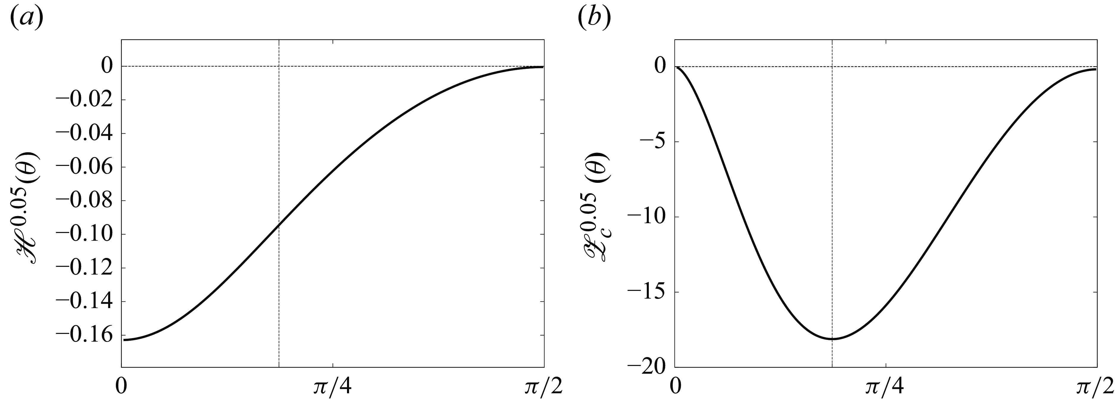
Figure 16. Graph of (a) ${\mathscr{H}}^{\varepsilon _3}(\theta )$ and (b) ${\mathscr{Z}}^{\varepsilon _3}_c(\theta )$ for the five-vortex problem with the parameters $\alpha = -2.05$ and $\beta = 0.5$ . The vertical line describes the angle for which ${\mathscr{Z}}^{\varepsilon _3}_c$ gets its minimum.

5. Concluding remarks

We have numerically investigated the dynamics of point-vortex solutions to the 2-D Euler- $\alpha$ equations with the initial data for which the solution to the PV system leads to self-similar collapse in a finite time. In particular, we have considered the three-, four- and five-vortex problems in which we have explicit formulae of self-similar collapsing solutions. The preceding results have already proven that the solution to the FPV system with that initial data converges to a self-similar collapsing orbit in the three-PV system and dissipates the enstrophy by the triple collapse in the $\varepsilon \to 0$ limit. In this paper, we have numerically shown that the enstrophy dissipation by collapse of point vortices could occur for the four- and five-vortex problems of the $\alpha$ -PV system in that limit by visualising the detailed processes of the vortex dynamics and the induced enstrophy variation in the limit, which has never been shown in the preceding results and has given a new insight into the mechanism of the enstrophy dissipation. Our result insists that the anomalous enstrophy dissipation by vortex collapse is not specific to three vortices and it could be universal mechanism for multiple vortices in 2-D inviscid flows. We have also shown that enstrophy dissipation is mainly caused by the interaction of point vortices with the negative interactive energy by comparing the total enstrophy, its variational part and the Hamiltonian energy of the FPV system.

We make some remarks and mention future directions. Our numerical computations have shown that, for some initial data leading to self-similar collapse in the PV system, the corresponding filtered point vortices converge to a collapsing orbit, but the mass of the enstrophy variation is not negative. Although, we have numerically suggested that the configuration of filtered point vortices at the critical time and the sign of the Hamiltonian energy are essentially related to the sign of the mass, further mathematical analysis is required to interpret this phenomenon physically and show the robustness of the enstrophy dissipation against the vortex strength. It is also necessary to investigate whether or not the same result holds for other filtered models such as the vortex blob regularisation and the exponential filter, and how differences among these models appear. It is challenging to find the enstrophy dissipating solutions for $N$ -vortex problems with $N \geqslant 6$ , and computing the multiple FPV system accurately is a difficult problem due to numerical errors induced by nonlinear effects of the system. Another direction of future works is considering the filtered model with periodic boundary conditions. Indeed, O’Neil (1989) has shown examples of a periodic array of point vortices leading to self-similar collapse. It is interesting to observe the dynamics of them in the periodic filtered model. We are also studying the inviscid limit of the 2-D Navier–Stokes equations with point-vortex initial vorticity. Gallay (2011) has proven that, for given initial profile of point vortices, the solution to the 2-D Navier–Stokes equations converges to the solution to the PV system with the same initial data in the inviscid limit except for the collapse time. Although it seems to be difficult to show the convergence at the collapse time, it is challenging to investigate whether the enstrophy dissipation by vortex collapse occurs in the inviscid limit or not.