Experimental investigation of inertial spheres settling in surface gravity waves

Abstract

We investigate the motion of weakly negatively buoyant spheres settling in surface gravity waves using laboratory experiments. The trajectories of the settling spheres are tracked over most of the water depth with simultaneous measurements of the background fluid flow. These experiments are conducted in the regime relevant for environmental and geophysical applications where both particle inertia and fluid inertia are important. Using these data, we show that the sphere motion is well described by the kinematic sum of the undisturbed fluid velocity and the particle terminal settling velocity as long as the fluid inertia is not too large. We show how this result can be understood in the context of an ad hoc Maxey–Riley–Gatignol-type equation where the drag on the particle is given by the Schiller–Naumann drag correlation. We also evaluate whether inertial particles experience enhanced settling in waves, finding that measurement uncertainties in the particle terminal settling velocity and the presence of Eulerian-mean flows do not allow the small percentage increase in the settling velocity to be measured. When the fluid inertia becomes large enough, we observe path instabilities caused by particle wake effects in both quiescent and wavy conditions. However, the particle velocity fluctuations associated with the path instabilities are unaffected by the background flow. The minimal influence of the wavy flow on the particle path instabilities is thought to be due to the large-scale separation between the waves and the particle.

1. Introduction

Particle motion is important in environmental and geophysical applications because it determines the transport of nutrients, pollutants and carbon in lakes and oceans (e.g. Moulton et al. 2022; Sutherland et al. 2023). These particles (e.g. plankton, (micro)plastics, marine aggregates, sediment) often exist in the regime where their size and density differences with respect to the flow length scale and fluid density, respectively, are both small. This makes the Basset–Boussinesq–Oseen (BBO) and Maxey–Riley–Gatignol (MRG) equations an attractive framework to model the particle dynamics since they take into account how the particle’s inertia modifies its transport and predict, for example, how the particle settling rate is affected.

Most relevant to this study, there have been a number of investigations into how particle settling is affected by the coupling between particle inertia and flow in surface gravity waves using theoretical expansions and numerical solutions of BBO- and MRG-type equations (e.g. Eames 2008; Santamaria et al. 2013; Bakhoday-Paskyabi 2015; DiBenedetto, Clark & Pujara 2022) and measurements in laboratory experiments (e.g. Clark et al. 2020). Some of these investigations reported enhanced particle settling and dispersion due to the coupling between particle inertia and wave-induced flow, with settling velocity up to 20 % greater than the particle terminal settling velocity in quiescent fluid.

While the BBO and MRG equations are derived under the assumption that the Reynolds number of the relative motion between the particle and the fluid is small, DiBenedetto et al. (2022) demonstrated that in many applications involving particle settling in surface waves, this Reynolds number is not necessarily small and can be as large as $10^3$ . In this range of particle Reynolds number, a common ad hoc extension of the BBO- and MRG-type equations uses the Schiller–Naumann drag correlation to estimate the drag force on the particle (Balachandar 2024). Additionally, in practical applications where fluid velocity fields are not available at a fine enough resolution, or where computational costs need to be reduced, particle motion is often approximated in an ad hoc manner as the kinematic sum of the background fluid velocity and the particle’s terminal settling velocity. However, predictions of particle trajectories from such ad hoc models are rarely tested against experimental data for particle settling at large particle Reynolds number.

Apart from the geophysical and environmental applications mentioned above, an investigation of inertial particles settling in surface waves is also attractive from a fundamental point of view. Surface waves offer a naturally two-dimensional, unsteady and non-uniform flow, where the flow field varies over a single length and time scale. While the flow is irrotational, limiting the scope of flow–particle interactions, this does provide certain advantages. In particular, the Saffman lift forces are absent (Balachandar 2024), and the Faxén corrections are irrelevant (DiBenedetto et al. 2022). Furthermore, in the laboratory it is possible to obtain well-resolved simultaneous measurements of settling particle trajectories and the background fluid flow with a single camera.

Finally, it is known that particles settling at large enough particle Reynolds number in quiescent fluid can have path instabilities that include lateral motions and rotations. The path instabilities for weakly negatively buoyant particles settling in otherwise quiescent fluid at different particle Reynolds numbers have been explored via numerical simulations (Jenny, Dušek & Bouchet 2004; Zhou & Dušek 2015) and laboratory experiments (Veldhuis & Biesheuvel 2007; Horowitz & Williamson 2010; Raaghav, Poelma & Breugem 2022; Cabrera-Booman, Plihon & Bourgoin 2024). The path instabilities emerge as the effects of fluid inertia break the axial symmetry in the particle wake, which leads to asymmetric forces and torques (Horowitz & Williamson 2010; Ern et al. 2012). However, for particles settling in an unsteady and non-uniform background flow, it remains unclear whether the presence and structure of these path instabilities would be modified through interaction with the flow.

In this paper, we investigate how inertia (due to both the particle and the fluid) affects the motion of weakly negatively buoyant particles settling in surface gravity waves. We do this via experiments where the motion of inertial spheres settling in a wavy flow is measured simultaneously with the background flow field. We compare the experimental data with predictions from an ad hoc MRG-type equation that uses the Schiller–Naumann drag correlation, and examine how this comparison varies with different dimensionless parameters. We check whether enhanced settling can be observed in the data, and whether path instabilities in the particle motion are modified by the wavy flow. The remainder of the paper is organised as follows. Section 2 gives a description of the relevant dimensionless parameters and the dynamics of particle motion. Section 3 describes the laboratory experiments, with the particle motion analysis given in § 4. We end with a summary of the main points and directions for future work in § 5.

2. Theoretical background

2.1. Surface waves

In small-amplitude (linear) wave theory, the dimensionless free-surface displacement for monochromatic progressive waves is given by $\eta = ka \cos (x-t)$ , and the dimensionless velocity field is given by

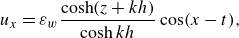(2.1a) \begin{align} u_x=\varepsilon _w \frac {\cosh (z+kh)}{\cosh {kh}}\cos (x-t), \end{align}

(2.1b) \begin{align} u_z=\varepsilon _w \frac {\sinh (z+kh)}{\cosh {kh}}\sin (x-t), \end{align}

where $\varepsilon _w = ka/\tanh {kh}$ is the wave nonlinearity parameter. Here, $a$ is the wave amplitude, $k$ is the wavenumber, $\omega$ is the wave angular frequency, and $h$ is the undisturbed water depth. The dimensionless coordinates $x$ and $z$ point in the direction of wave propagation and upwards against gravity, respectively, with the origin of $z$ being at the undisturbed free surface. All variables are made dimensionless using the wavenumber $k$ and angular frequency $\omega$ .

2.2. Dimensionless parameters

The parameters that characterise the settling of small, weakly negatively buoyant spheres in surface gravity waves are as follows. The flow field in small-amplitude surface gravity waves is characterised by three length scales, namely the wavelength $L$ (or wavenumber $k = 2\unicode{x03C0} /L$ ), the wave amplitude $a$ , and the water depth $h$ , and by a single time scale, the wave period $T$ (or angular frequency $\omega = 2\unicode{x03C0} /T$ ). The spherical particle is characterised by its density $\rho _p$ , diameter $d_p$ , and terminal settling velocity in quiescent fluid $v^{\prime }_s$ . Together with the fluid properties (namely, density $\rho$ and kinematic viscosity $\nu$ ), and the gravitational acceleration $g$ , there are a total of ten dimensional variables and three fundamental dimensions, which yields seven independent dimensionless parameters. Note that the need to include $v^{\prime}_s$ as an additional parameter arises since its value cannot be determined from other variables when the particle Reynolds number is not small such that the settling velocity is no longer given by the classical Stokes settling velocity. Additionally, the gravitational acceleration is implicitly included in the variables describing the waves since it links the wave period and water depth to the wavelength via the dispersion relation ( $\omega ^2 = gk \tanh kh$ ), but it needs to be included separately when considering particle settling in waves due to its role in the vertical dynamics of particle motion.

We choose the seven dimensionless parameters as follows. The wave-induced flow is characterised by the wave steepness $ka$ and the relative water depth $kh$ . The particle settling in quiescent fluid is characterised by the specific gravity $\gamma = \rho _p/\rho$ and the terminal settling velocity particle Reynolds number ${\textit {Re}}_{p,t} = v^{\prime}_s d_p/\nu$ , which quantifies the importance of fluid inertia. Note that since the terminal settling velocity is not known a priori, a better indicator of the importance of fluid inertia, instead of $Re_{p,t}$ , is the Galileo number ${\textit{Ga}} = v^{\prime}_g d_p/\nu$ , where the characteristic settling velocity is the inertia-gravitational velocity scale $v^{\prime}_g = {((\gamma -1) gd_p)^{1/2}}$ . We will use both dimensionless numbers as appropriate, but only one of them should be included in the list of seven dimensionless parameters.

For the remaining three dimensionless parameters, we choose to characterise the interaction between the particle and wave-induced flow by the ratios of length, time and velocity scales between the particle and the fluid, given respectively by

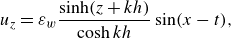
(2.2) \begin{equation} {{Sz}} = kd_p, \quad {{St}} = \frac {\omega d_p^2 (\gamma +C_m)}{18\nu (1+0.15\, Re_{p,t}^{0.687})} (=\omega \tau _{p,SN}), \quad {{Sv}} = \frac {v^{\prime}_s}{gka/\omega }. \end{equation}

Here, ${\textit{Sz}}$ is the size number, which quantifies the ratio between the particle diameter ( $d_p$ ) and the wavelength ( $L$ ); ${\textit{St}}$ is the Stokes number, which quantifies the particle inertia via the ratio between the time scale for an inertial particle to relax to the flow using the Schiller–Naumann drag correlation ( $\tau _{p,SN}$ ) and the wave period ( $T$ ); and ${\textit{S}v}$ is the settling number (sometimes called the Rouse number), which quantifies the importance of gravitational settling via the ratio between the particle terminal settling velocity ( $v^{\prime}_s$ ) and the characteristic velocity scale of fluid motion in waves ( $u_w=gka/\omega$ ). In the particle time scale, the added mass coefficient for a sphere is taken to be $C_m = {1}/{2}$ , and the particle Reynolds number is determined based on the terminal settling velocity.

2.3. Particle motion under the MRG framework

A widely used simplified version of the MRG equation (without the history force and Faxén corrections, e.g. see Maxey & Riley 1983; Bergougnoux et al. 2014; DiBenedetto et al. 2022) is given in dimensionless form by

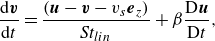(2.3) \begin{equation} \frac {{\rm d}\boldsymbol{v}}{{\rm d}t} = \frac {(\boldsymbol{u} - \boldsymbol{v} - v_s \boldsymbol{e}_z)}{{\textit{St}}_{{lin}}} + \beta \frac {{\rm D}\boldsymbol{u}}{{\rm D}t}, \end{equation}

where all variables are made dimensionless using $k$ and $\omega$ . Here, $\boldsymbol{v}$ is the particle velocity, $\boldsymbol{u}$ is the undisturbed fluid velocity, $v_s$ is the dimensionless terminal settling velocity, $\boldsymbol{e}_z$ is the unit vector antiparallel to gravity, and $\beta = ({1 + C_m})/({\gamma + C_m})$ . The term on the left-hand side signifies the particle acceleration, the first term on the right-hand side signifies the combined forces of drag and buoyancy, and the second term on the right-hand side signifies the forces due to added mass and fluid acceleration (Bergougnoux et al. 2014). To emphasise that the particle motion is in the small particle Reynolds number regime, the particle Stokes number is written as ${\textit{St}}_{{lin}}=\omega \tau _{p,\textit{lin}}$ where ‘lin’ refers to the fact that the (Stokes) drag is linear with respect to the slip velocity. The particle relaxation time scale is given by $\tau _{p,\textit{lin}} = d_p^2 (\gamma +C_m)/18\nu$ , and the dimensional terminal settling velocity is given by the classical Stokes settling velocity $v^{\prime}_{s} = \tau _{p,\textit{lin}}(1-\beta )g$ .

In the limit of small and weakly negatively buoyant particles ( $(1 - \beta ) \rightarrow 0,\ {\textit{St}} \rightarrow 0$ ), the equation reduces to the simple kinematic model

(2.4) \begin{equation} \boldsymbol{v} = \boldsymbol{u} - v_s \boldsymbol{e}_z, \end{equation}

where the particle velocity is the sum of the undisturbed fluid velocity at the particle position and the particle terminal settling velocity. In this state, the particle drag force and buoyancy are the only forces in play, and they are in balance. When ${\textit{St}}$ is small but finite, a kinematic solution for particle motion can be obtained from an ${\textit{St}}$ expansion. However, for larger or denser particles, an increase in ${\textit{St}}$ (quantifying particle inertia) is also accompanied by an increase in particle Reynolds number (quantifying fluid inertia) since larger particle size and density also result in faster relative motion between the fluid and the particle. This can render the problem outside the bounds of validity of the MRG formulation since the relative motion between the particle and the fluid is no longer characterised by a low Reynolds number.

Bergougnoux et al. (2014) investigated the applicability of (2.3) and (2.4) for particle settling based on laboratory experiments of spheres settling in a two-dimensional, steady cellular flow. Comparing particle trajectories from the full MRG equation ((2.3) with the history force and Faxén corrections included) with experimental data, they found that the motion of settling particles at low Stokes numbers ( ${\textit{St}} \lesssim 0.1$ ) and finite particle Reynolds numbers ( ${\textit {Re}}_{p,t} \lesssim 10$ ) was well predicted by the simple kinematic model (2.4). This was true as long as one used the measured settling velocity rather than the classical Stokes settling velocity. However, as Bergougnoux et al. (2014) noted, the applicability of (2.3) and (2.4) for larger particle diameters and densities is questionable since the larger Stokes numbers (quantifying particle inertia) would also be accompanied by larger particle Reynolds numbers (quantifying fluid inertia).

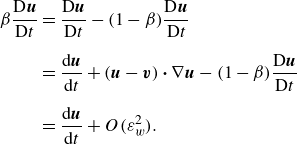
DiBenedetto et al. (2022) used an ad hoc form of the MRG equation to study particle settling in waves that takes the dimensionless form

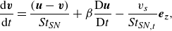(2.5) \begin{equation} \frac {\mathrm{d}\boldsymbol{v}}{\mathrm{d}t} = \frac {(\boldsymbol{u} - \boldsymbol{v})}{\textit{St}_{\textit{SN}}} + \beta \frac {\mathrm{D}\boldsymbol{u}}{\mathrm{D} t} - \frac {v_{s}}{{\textit{St}_{\textit{SN}}}_{,t}} {\boldsymbol{e_{z}}} , \end{equation}

where the Stokes number based on the Schiller–Naumann drag correlation is given by ${\textit{St}}_{\textit{SN}} = {\omega d_p^2(C_m+\gamma )}/{[18\nu (1+0.15\, {\textit{Re}}_p^{0.687})]}$ and ${\textit{St}}_{{\textit{SN},t}}$ is the same quantity replacing ${\textit {Re}}_p$ with ${\textit {Re}}_{p,t}$ . Using the Schiller–Naumann drag correlation to approximate the drag force for ${\textit {Re}}_p \lesssim 10^3$ yields a modified definition of the particle Stokes number, denoted as ${\textit{St}}_{\textit{SN}}$ , where the subscript SN indicates the use of the Schiller–Naumann drag model. While $\textit{St}_{\textit{SN}}$ is a dynamic quantity that evolves as the particle travels through the flow, ${\textit{St}_{\textit{SN}}}_{,t} = \omega d_p^2 (C_m + \gamma )/[18\nu (1 + 0.15\, {\textit {Re}}_{p,t}^{0.687})]$ is constant. Here, ${\textit{S}v}$ appears implicitly in the dimensionless particle terminal settling velocity since it can be written as $v_s = \varepsilon _w \, {\textit{S}v}$ .

DiBenedetto et al. (2022) derived an explicit expression for the particle velocity based on an expansion in ${\textit{St}}$ to quantify effects of particle inertia, and used a multiple time scale analysis to obtain the wave-averaged particle drift velocity. They also discussed the mechanisms for enhanced settling and dispersion of inertial particles in waves, extending the Santamaria et al. (2013) results to arbitrary depth ( $kh$ value) and drag force that is nonlinear with respect to the particle slip velocity using the Schiller–Naumann drag correlation.

3. Laboratory experiments

We conducted experiments in a rectangular tank that was 504 cm long, 50 cm deep, and 20 cm wide, constructed with glass walls mounted on a steel frame, as shown in figure 1. The water depth was $h=31.5$ cm, with water temperature $21\,^\circ\text{C}$ (kinematic viscosity $\nu = 9.78 \times 10^{-7}$ m $^2$ s⁻¹). The coordinates $(x^{\prime}, z^{\prime})$ are aligned with the wave propagation and antigravity directions, respectively, with the origin at the still-water level 2.5 m downstream of the wavemaker. Triangular prisms of coarse-pored sponges were placed at both ends of the tank to dissipate wave energy and limit reflection. To generate waves, we used a cylindrical plunging wavemaker with diameter 7.4 cm, and a right-angled triangular plunging wavemaker with dimensions 24 cm (height) by 15 cm (length). Below, the primed quantities refer to dimensional quantities, with the unprimed counterpart referring to its dimensionless version.

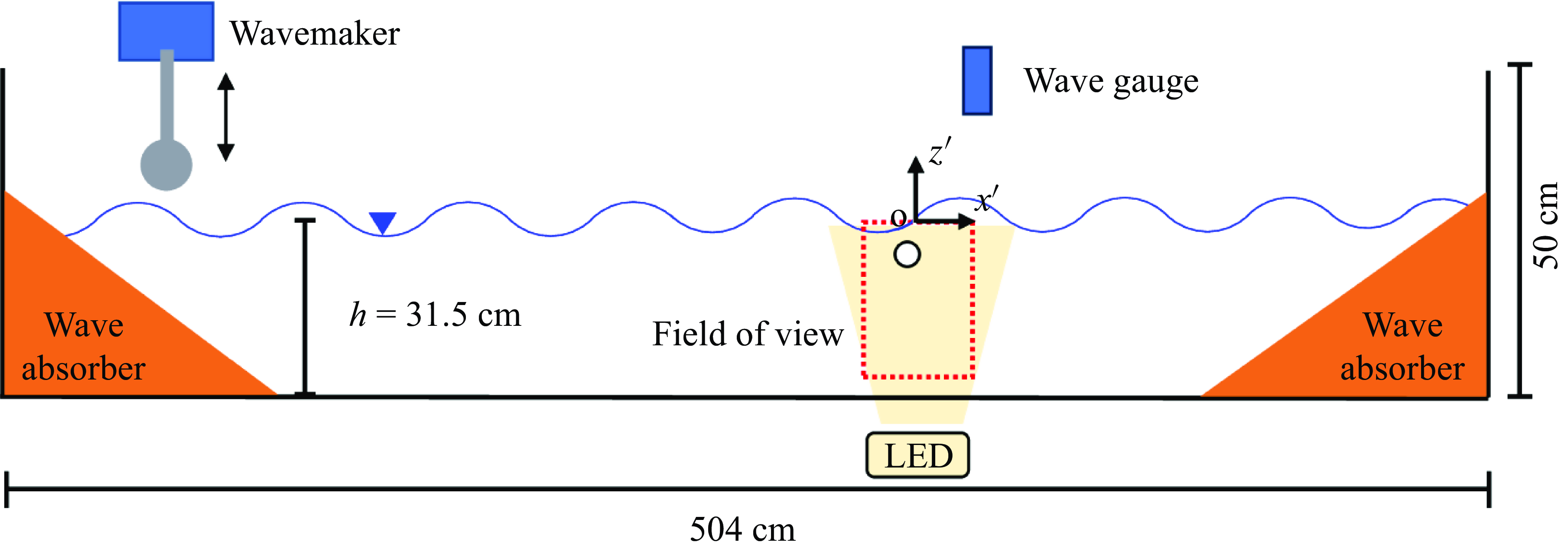
Figure 1. Schematic of the experimental set-up.

3.1. Waves and wave-induced flow

The waves and wave-induced flow were characterised as follows. A wave gauge (Toughsonic 3, Senix Corporation) was used to measure the free surface displacement time series $\eta ^{\prime}(t^{\prime})$ . The wave angular frequency $\omega$ was found from the location of the peak in the spectrum of the wave gauge data. The wave amplitude $a$ was estimated by fitting the data to $\eta^{\prime} = a \cos \omega t^{\prime}$ , allowing for an arbitrary phase shift. Finally, the wavenumber $k$ was calculated from the dispersion relationship $\omega ^2 = gk\tanh {kh}$ . 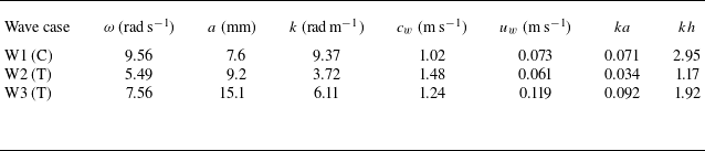Table 1 summarises the wave characteristics and dimensionless wave parameters for each wave case, including the wave speed $c_w$ , characteristic wave-induced fluid velocity $u_w = gka/\omega$ , wave steepness $ka$ , and relative depth $kh$ .

Table 1. Parameters of each wave case, where C and T in the wave case column indicate that waves are generated by the cylindrical and triangular wavemakers, respectively.

We measured the wave-induced flow using particle image velocimetry (PIV). The PIV field of view spanned 16.5 cm in the $x^{\prime}$ direction, and 26 cm in the $z^{\prime}$ direction, covering 80 % of the water depth over $-26\ \text{cm}\lt z^{\prime}\lt 0$ . No measurements were made in the bottom 5.5 cm of the water column. It was illuminated with an LED line light with average light sheet thickness 1 cm, and seeded with tracer particles ( $d_{50} = 10 \unicode{x03BC}$ m, $\gamma = 1.1$ ; 110P8 Potter Industries). We took images at 20 Hz with a camera (LaVision Imager MX 2M-160, 1936 $\times$ 1216 px) fitted with a 16 mm lens (Tamron) to get magnification factor 7.14 px $\text{mm}^{-1}$ . To obtain the flow velocity field, we used a PIV algorithm with an iterative multi-pass cross-correlation method (DaVis v10.2; LaVision), where the last pass used 64 $\times$ 64 px with 50 % overlap and a Gaussian fit for subpixel accuracy. The final velocity vectors had spatial resolution approximately 4.5 mm, and were checked for quality by examining the relative heights of the first and second correlation peaks. Low-quality vectors ( $\lt 2\, \%$ ) were removed without interpolation. For wave cases W1 and W2, the reflection of the moving water surface on the flume side wall contaminated the image data near the surface. For wave case W3, the vertical gradients in the flow were large, and the flow near the moving surface resulted in tracer streaks. Despite these challenges, we were able to obtain velocity data for all wave cases below depth $z^{\prime} \lesssim -3a$ (figure 2).

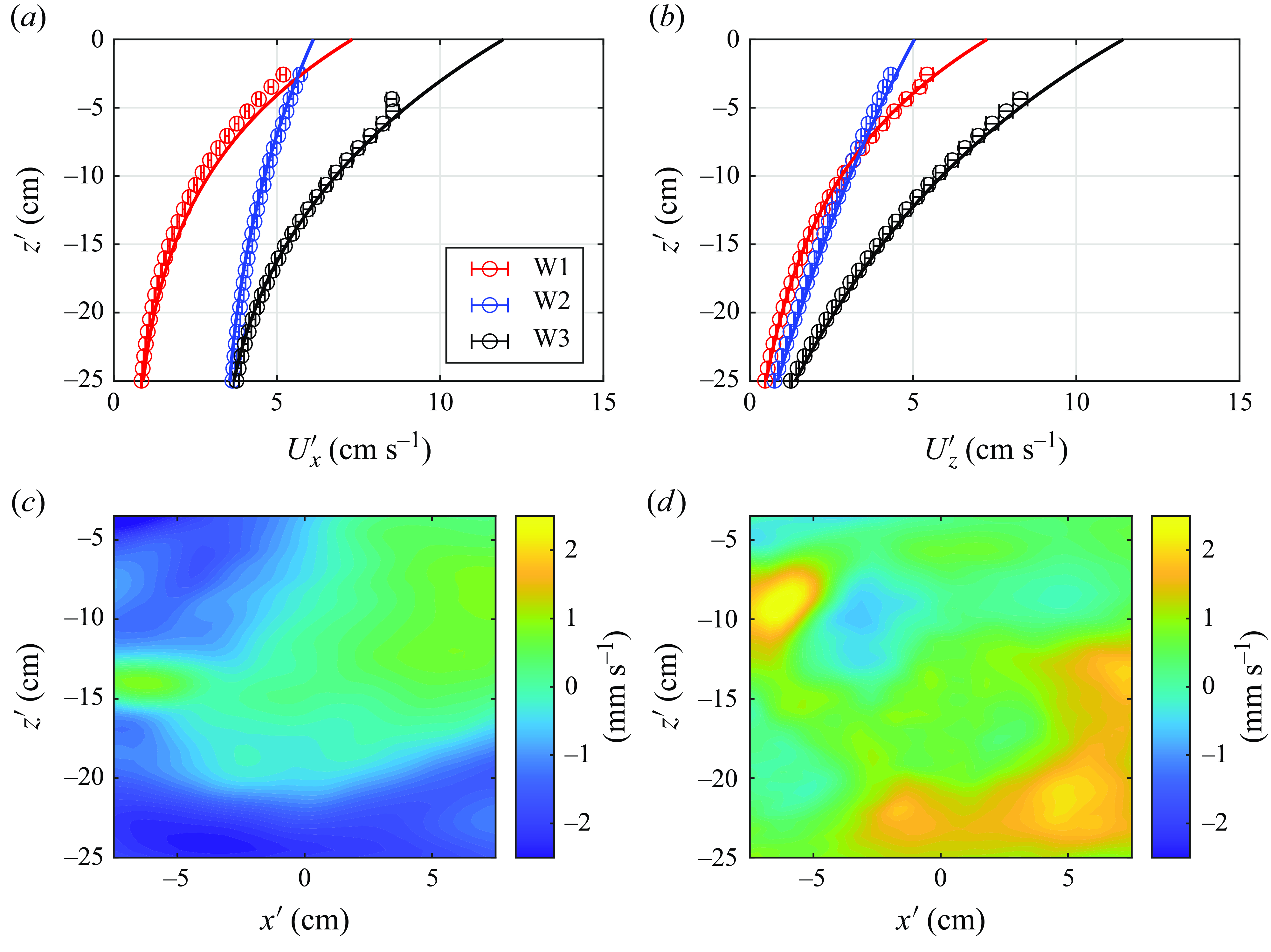
Figure 2. Wave-induced flow spanning $-26\ \text{cm}\lesssim z^{\prime} \lesssim -3a$ . (a,b) Velocity amplitude profiles for oscillatory flow; data with 95 % confidence intervals (circles) and linear wave theory (solid lines). (c) Horizontal Eulerian-mean flow (W1), $\overline {U}^{\prime}_x$ . (d) Vertical Eulerian-mean flow (W1), $\overline {U}^{\prime}_z$ .

To evaluate whether the wave-induced flows conform to linear wave theory (2.1), we compared the PIV velocity measurements with the dimensional velocity field given by

(3.1a) \begin{align} u^{\prime}_x = U^{\prime}_x(z^{\prime}) \cos (kx^{\prime}-\omega t^{\prime}) + \overline {U}^{\prime}_x, \end{align}

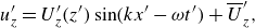(3.1b) \begin{align} u^{\prime}_z = U^{\prime}_z(z^{\prime}) \sin (kx^{\prime}-\omega t^{\prime}) + \overline {U}^{\prime}_z, \end{align}

where $U^{\prime}_x(z^{\prime})$ and $U^{\prime}_z(z^{\prime})$ denote the oscillatory velocity amplitudes in the horizontal and vertical directions, respectively, and $\overline {U}^{\prime}_x$ and $\overline {U}^{\prime}_z$ represent the Eulerian-mean velocities in the horizontal and vertical directions, respectively. For pure monochromatic progressive waves, $U^{\prime}_x(z^{\prime}) = (gka/\omega )\cosh (k(z^{\prime}+h))/\cosh kh$ and $U^{\prime}_z(z^{\prime}) = (gka/\omega )\sinh (k(z^{\prime}+h))/\cosh kh$ , and $\overline {U}^{\prime}_x=\overline {U}^{\prime}_z=0$ . Figure 2 displays the wave-induced velocity amplitudes for wave cases W1–W3, and the Eulerian-mean flow field for wave case W1, obtained from the experimental data by fitting the velocities at each PIV grid point to (3.1). The velocity amplitudes are averaged in the horizontal direction, with the 95 % confidence intervals calculated using the bootstrap technique. The velocity amplitudes show good agreement with linear wave theory, except for a small deviation near the free surface. Furthermore, the magnitudes of Eulerian-mean flow are small compared to the amplitudes of the oscillatory flow.

3.2. Particle settling

We measured the settling dynamics of five solid spherical particles whose properties are summarised in table 2. The nylon (N1, N2, N3) and Torlon (T1) particles were purchased (US Plastics Corp.), whereas the nylon 12 particles (N4) were 3-D printed (selective laser sintering, Fuse 1, Formlabs). We checked that the manufacturer’s reported particle diameters ( $d_p$ ) were accurate to the resolution of standard callipers. Since particle mass (and density) are expected to be altered by water absorption, we stored the particles in water before and in between experiments. The particle mass was then measured using a precision balance scale, allowing us to calculate the particle density ( $\rho _p$ ) and the relative density ( $\gamma$ ).

Table 2. Dimensional particle parameters. Uncertainty bounds show the 95 $\%$ confidence intervals using the bootstrap method.

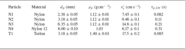
We measured the terminal settling velocity ( $v^{\prime}_s$ ) of each particle with 10 repetitions by particle tracking (described below) in quiescent water in the same tank. We also estimated the particle relaxation time scale using the Schiller–Naumann drag correlation $\tau _{p,SN}=d^2_p(\gamma +({1}/{2}))/[18\nu (1+0.15\, Re_{p,t}^{0.687})]$ . Data from particles settling in quiescent fluid showed that the particle vertical velocities reached the terminal settling velocities over a time that was $O(\tau _{p,SN})$ , similar to the exponential approach to the terminal settling velocity in the Stokes drag regime. Thus, we concluded that $\tau _{p,SN}$ provides a reliable estimate for the particle relaxation time scale of our inertial particles.

For N4 particles, the mass measurements were less reliable due to variability in water adherence. So we estimated its relative density from the measured terminal settling velocity, solving for $\gamma$ in $v^{\prime}_s = \sqrt {(4/3) (\gamma - 1)d_p g/C_D}$ , where $C_D=(24/Re_{p,t})(1+0.15\,Re_{p,t}^{0.687})$ is the Schiller–Naumann correlation for the drag coefficient.

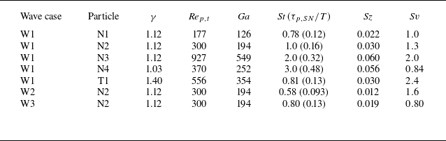
Table 3 lists all experiments for particles settling in waves with the relevant dimensionless parameters. In all cases, the particles are small compared to the wavelengths so that the size number is small ( ${\textit{Sz}} \ll 1$ ), and the particles are weakly negatively buoyant so that the specific gravity is just above unity, $(\gamma - 1) \ll 1$ , with the possible exception of T1 particles, where $(\gamma - 1) = 0.4$ . However, the particle relaxation time scale is not small compared to the wave period, and the Stokes number is ${\textit{St}} =O(1)$ . The settling number covers the range $0.8 \leqslant Sv \leqslant 2.4$ , with values below, at and above unity. The $Re_{p,t}$ and $\textit{Ga}$ values span a range that includes particles both below the threshold for path instabilities (N1) and above the threshold for path instabilities (N2–N4, T1).

Table 3. Dimensionless parameters for each experiment. Ratios of the particle relaxation time to the wave period ( $\tau _{p,SN}/T$ ) are also presented, alongside ${\textit{St}}$ .

3.2.1. The N1, N2, N3, N4 and T1 particles in wave case W1

Experiments with N1, N2, N3, N4 and T1 particles in wave case W1 were used to investigate the particle settling dynamics at different Galileo numbers ( $126 \leqslant {\textit{Ga}} \leqslant 549$ ) at ${\textit{St}} = O(1)$ ( $0.78 \leqslant {\textit{St}} \leqslant 3.0$ ) and ${\textit{S}v} = O(1)$ ( $0.84 \leqslant {\textit{S}v} \leqslant 2.4$ ). To gather data for particle settling dynamics, we simultaneously tracked the spheres and measured the velocity field using a combined particle tracking and PIV approach.

In each experiment, a single sphere was released with a tweezer at approximately 1 cm below the wave trough once the waves were established. We followed this procedure after preliminary experiments suggested that if a particle is dropped from above the water surface, then its initial velocity in the water may exceed its terminal settling velocity, and its trajectory may be altered by air bubbles trapped underneath the particle. The release points were confined to within a few centimetres of the origin in the horizontal direction.

We conducted 10 repetitions for N1, N3, N4 and T1 particles, and 25 repetitions for N2 particles (as detailed in § 3.2.2), varying the initial phase of the wave when the particle was dropped, and excluding drops where the particle travelled outside the light sheet in the spanwise direction. We waited at least 10 minutes between drops to minimise the influence of the previous drop. Occasionally, we had to remove settled particles from the tank before the next release, and this procedure likely altered the structure of the Eulerian-mean flow even though we waited approximately 30 minutes between releases in such cases.

To obtain particle trajectories from the image data, we first removed the background image over the set of images for each trajectory by subtracting the minimum count for each pixel. We determined the particle centroid in each image via the imfindcircles function in MATLAB, which employs a circular Hough transform, setting the radius range based on the expected particle size in pixels. This procedure had an uncertainty of 0.5 pixel ( $\approx 0.07$ mm), which was estimated by checking that circles with centroids shifted from the estimated centroid did not cover the entire particle in the image. Finally, a Savitzky–Golay filter (sgolayfilt in MATLAB) with a second-order polynomial was applied to the data to reduce noise in particle centroid positions. Particle velocities were then calculated using a first-order finite difference scheme using the filtered data. Using the finite difference scheme ensures that the particle velocity data are synchronised with the fluid velocity PIV data.

Since the filter performance depends on the fitting window $L_f$ , we compared the trajectories of the raw and filtered particle centroids for different $L_f$ for the N1 particle (figure 3 a). The filtered data with $L_f = 5$ help to reduce the noise in the particle centroid positions, but larger $L_f$ values change the particle positions more than the measurement uncertainty (0.5 pixel or 0.07 mm) (inset in figure 3 a). Additionally, the effect of filtering on particle velocity shows that using $L_f=5$ reduces noise, but further increases in $L_f$ result in excessive smoothing (figure 3 b). This is evident from the reduction in the magnitude of the velocity spectra at the peak (figure 3 c). Thus, we use $L_f = 5$ points across all data.

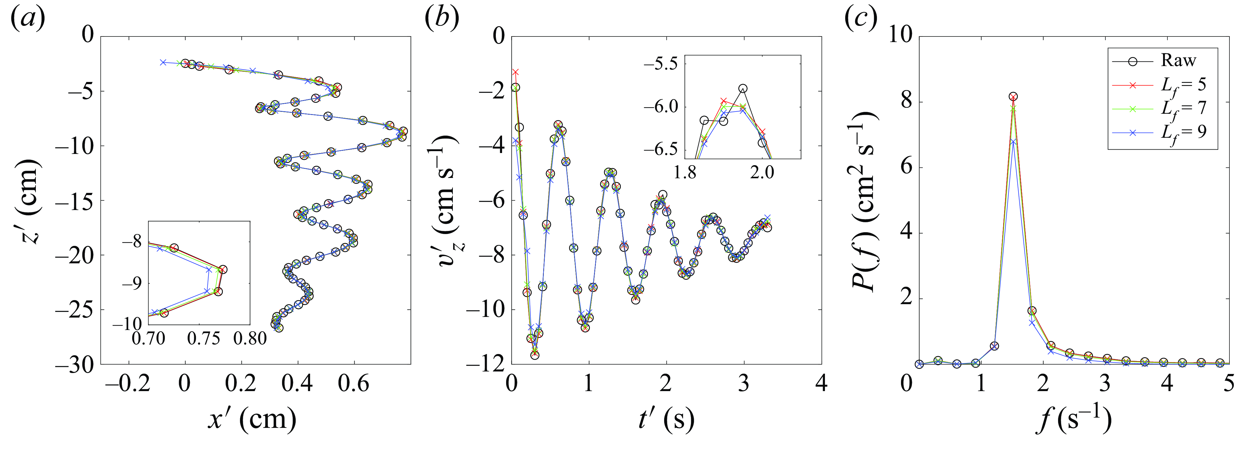
Figure 3. Representative raw and filtered data for N1 particles: (a) positions, (b) velocities, (c) velocity spectra. Insets offer close-up views.

The fluid velocity data were obtained using PIV (as described above), with low-quality vectors ( $\lt 2\, \%$ ) removed without interpolation, which also included vectors where the interrogation window overlapped with any portion of the settling particle. The undisturbed fluid velocity at the particle position was calculated with linear interpolation of the velocity vectors in space, using the particle position at the midpoint between successive images. Since the fluid velocity data are well resolved in space and time, the linear interpolation method was found to be sufficiently accurate. In the interpolation, we excluded fluid velocity vectors within a radius $3d_p$ from each particle centroid and from near the free surface ( $z^{\prime} \gtrsim -3a$ ).

We examined the effect of the exclusion radius on the interpolation; see the example of flow velocities at the particle position for an N3 particle (largest size and $\textit{Ga}$ ) in figure 4. The interpolated fluid velocity at the particle centroid is not sensitive to the size of the exclusion region at $3d_p$ or above. The maximum velocity difference between using exclusion radii $3d_p$ and $5d_p$ is approximately $10^{-3}$ , which is much smaller than the magnitude of the slip velocities (see figure 7(e) below). Thus, we concluded that an exclusion radius of $3d_p$ was sufficient to obtain the background fluid velocities at the particle centroid positions.

It is worth noting that while our experimental set-up allows us to obtain well-resolved simultaneous measurements of the particle trajectories and background fluid velocities over most of the water column, we are not able to capture the particle wake within the fluid since the light is delivered from below the tank, and the wake flow immediately above the particle is blocked by the particle. Some part of the wake structure may influence the fluid velocity vectors in the vicinity of the particle, but since the wake flow is not measurable, these vectors are excluded from the analysis as explained above.

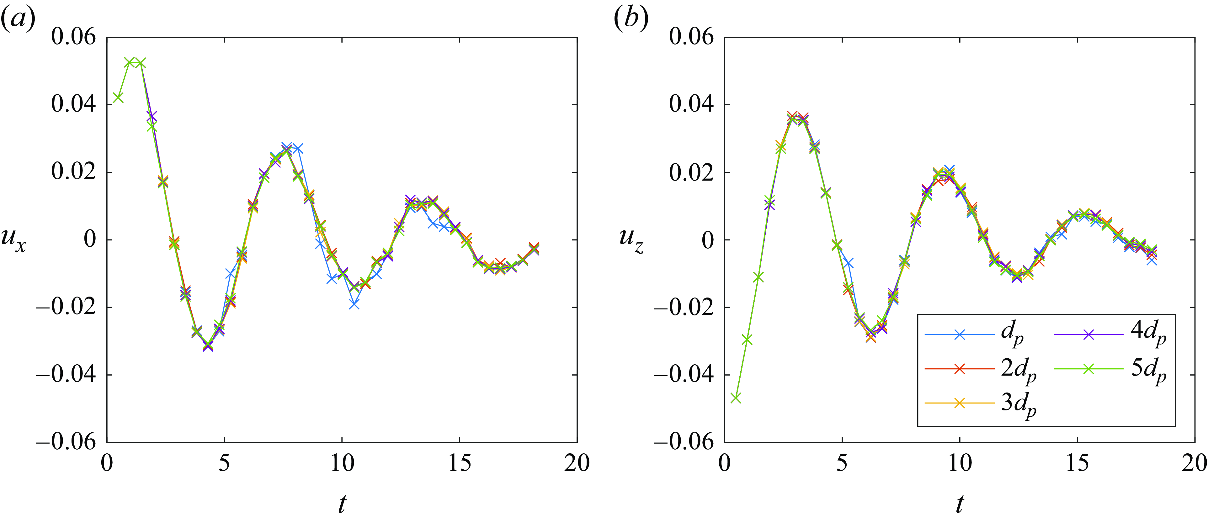
Figure 4. Representative dimensionless fluid velocities interpolated to the particle centroid for varying exclusion radius; N3 particle in wave case W1.

3.2.2. The N2 particles in wave cases W1, W2 and W3

Experiments with N2 particles in wave cases W1, W2 and W3 were used to investigate how the path instabilities of settling spheres in quiescent fluid would be affected by unsteady and non-uniform wavy flow. The N2 particles ( $\gamma = 1.12, \ {\textit{Ga}} = 194$ ) were chosen since their Galileo number is above the previously found threshold for steady vertical trajectories in quiescent fluid ( ${\textit{Ga}} \approx 155$ ). Across wave cases W1, W2 and W3, the wave frequency was varied to vary the flow time scale relative to the dominant time scale of the particles’ path instabilities. At the low frequencies of W2 and W3, we used the triangular wavemaker, as the cylindrical wavemaker was unable to produce waves without also increasing the amplitude (table 1). This resulted in some variation in ${\textit{S}v}$ in this experimental set, but all experiments were still at ${\textit{St}} = O(1)$ ( $0.58 \leqslant {\textit{St}} \leqslant 1.0$ ) and ${\textit{S}v} = O(1)$ ( $0.8 \leqslant {\textit{S}v} \leqslant 1.6$ ) (table 3). We conducted 25 repetitions for each wave condition and in quiescent conditions to reduce the statistical uncertainty in the results. Measurements of the flow and particle motion were made using the same methods as described in § 3.2.1.

4. Analysis of particle motion

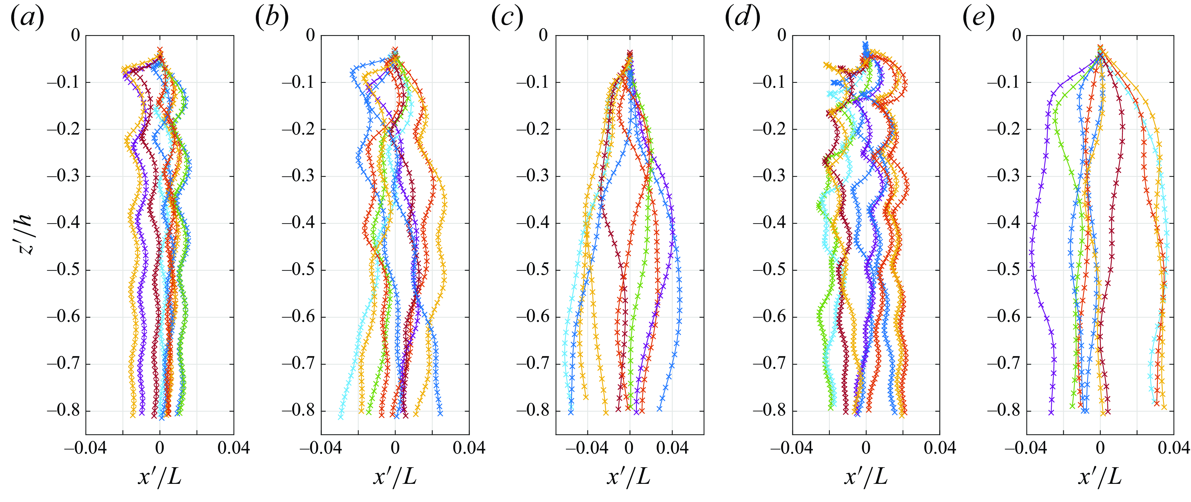
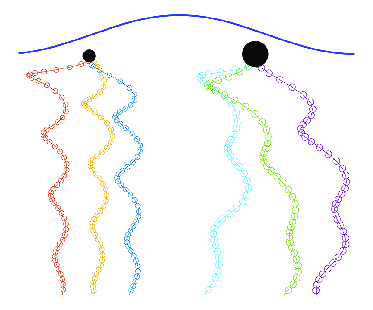
Figure 5. Particle trajectories in wave case W1 normalised by wavelength and water depth: (a) N1, (b) N2, (c) N3, (d) N4, (e) T1.

We begin with a qualitative examination of typical particle trajectories and particle velocities relative to the background flow, before proceeding to more quantitative analysis for different subsets of the data.

Figure 5 shows particle trajectories in wave case W1 (§ 3.2.1). The $x^{\prime}$ and $z^{\prime}$ coordinates are made dimensionless by the wavelength and water depth, respectively, and all trajectories are shown with initial horizontal position $x^{\prime}=0$ . The N1 particles, released at different wave phases, spread out immediately after release in the region $ -0.3 \leqslant z^{\prime}/h \leqslant 0$ , and later fall predominantly in the vertical direction, with small and regular horizontal oscillations in the region $z^{\prime}/h \leqslant -0.3$ . The horizontal oscillations decay as the particles settle deeper, and appear to be consistent in magnitude across different trajectories. In contrast, the trajectories of the other particles (N2–N4, T1) show larger horizontal motions than the N1 particles, with some particles (N3, T1) showing qualitatively different trajectories from the start. Notably, the horizontal motions do not seem to decay with depth.

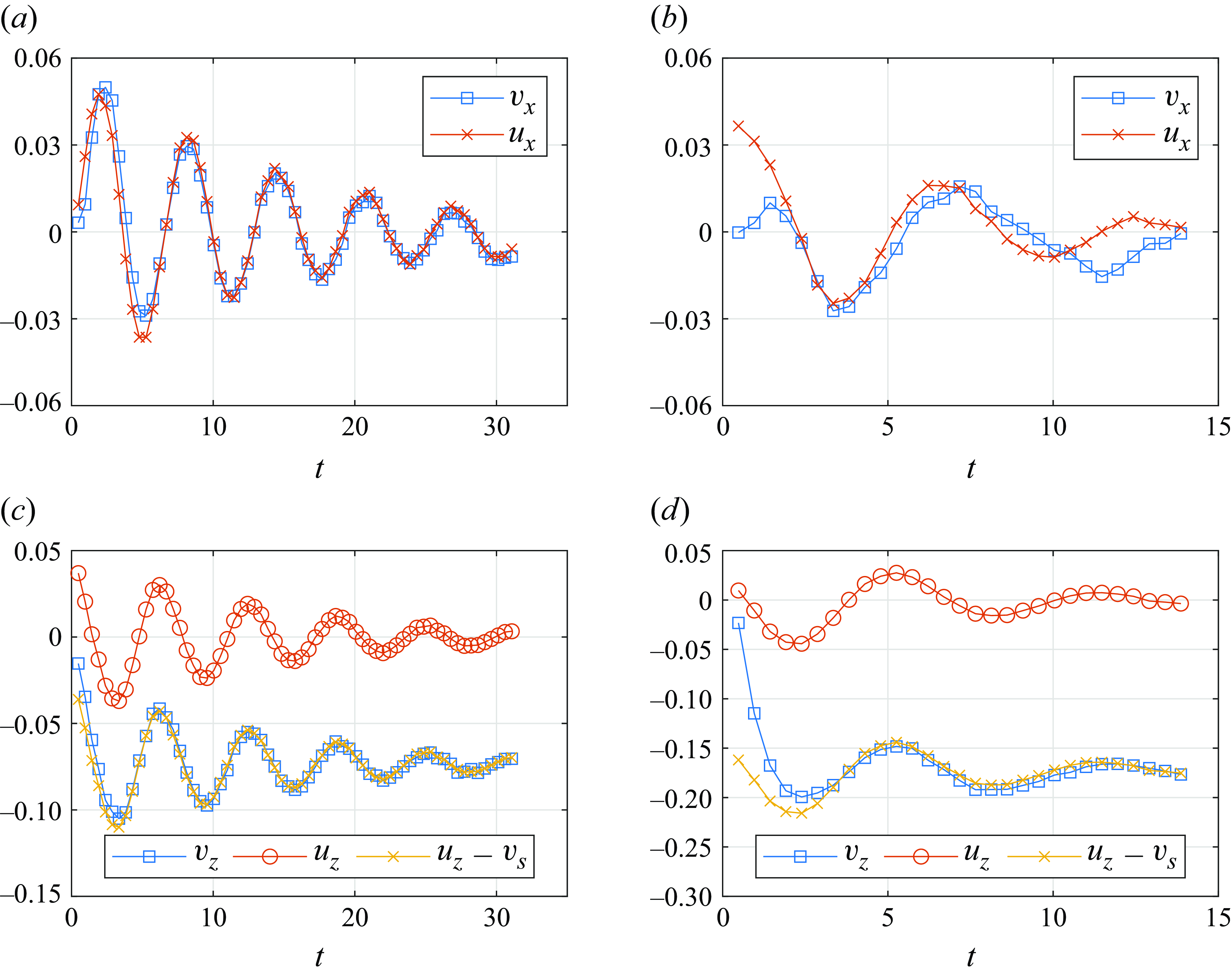
Figure 6. Representative normalised particle velocity ( $\boldsymbol{v}$ ) and normalised undisturbed fluid velocity ( $\boldsymbol{u}$ ) data: (a,c) N1, (b,d) T1, for (a,b) horizontal components, (c,d) vertical components, including the kinematic model ( $v_z = u_z-v_s$ ).

Moving on to the particle velocities, figure 6 shows typical time series of the dimensionless particle velocity and the corresponding dimensionless fluid velocity at the particle position for N1 and T1 particles. The wave-induced flow clearly affects the motion of both particles, but there are differences in the particle slip velocity (defined as $\boldsymbol{v}_{\textit{slip}} = \boldsymbol{v} - \boldsymbol{u}$ ). In particular, the particle velocities are well predicted by the kinematic model (see (2.4), $\boldsymbol{v}_{\textit{slip}} = -v_s \boldsymbol{e}_z$ ) for the N1 particle ( $\gamma = 1.12, \ {\textit{Ga}} = 126$ , ${\textit{St}} = 0.78$ ) in both directions after an initial transient period, whereas for the T1 particle ( $\gamma = 1.40, \ {\textit{Ga}} = 354$ , ${\textit{St}} = 0.81$ ), only the vertical velocity follows the kinematic model after an initial transient period, and the horizontal velocity continues to deviate from the undisturbed fluid velocity.

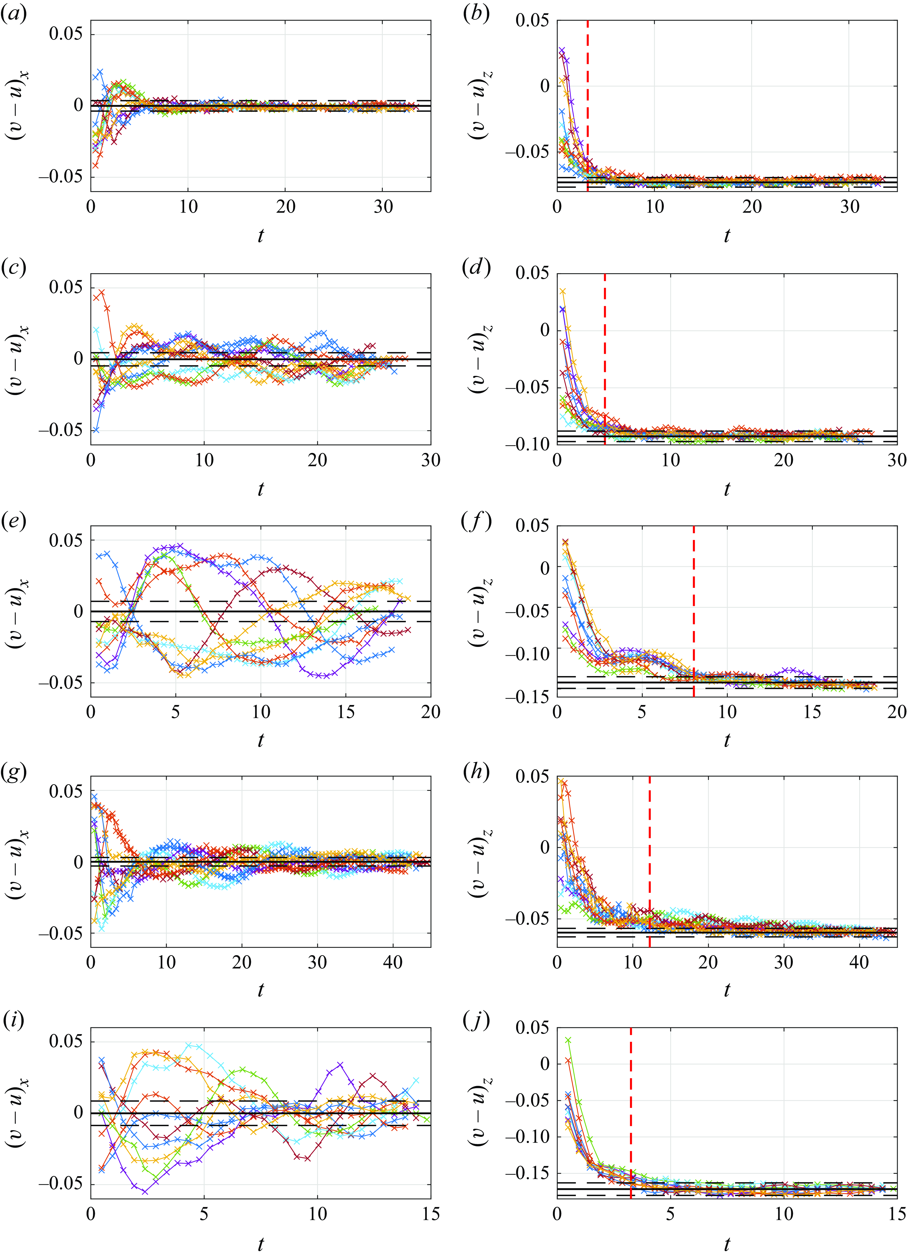
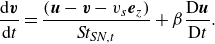
Figure 7. Particle slip velocities normalised by wave speed: (a,b) N1, (c,d) N2, (e,f) N3, (g,h) N4, (i,j) T1. Black solid lines are $(v-u)_x =0$ and $(v-u)_z = -v_s$ . Black dashed lines show $\pm 0.05v_s$ relative to the black solid lines. Red dashed lines represent $t = 4 \omega \tau _{p,SN}$ . The colours correspond to the slip velocity of the respective particles in figure 5.

To further examine whether particle velocity can be predicted by the kinematic model (2.4), we show data of particle slip velocity for all experiments in wave case W1 in figure 7. The data show that to a good approximation, the vertical slip velocities for all particles relax to the terminal settling velocity $(v_z-u_z) \approx -v_s$ , with fluctuations about this state that are small relative to the magnitude of $v_s$ . Further, all particles appear to reach this quasi-steady vertical slip at $t^{\prime} \approx 4\tau _{p,SN}$ after their release (red dashed lines), regardless of the initial conditions, similar to the exponential approach to terminal settling velocity in the Stokes drag regime. Together with the same observation in quiescent conditions, this observation shows that the particle time scale estimated using the Schiller–Naumann drag correlation serves as a reliable estimate for the particle relaxation time in both quiescent and wavy conditions. In contrast to the vertical slip velocities, the horizontal slip velocities show stark differences across different particles. While N1 particles reach a state where the horizontal slip velocity becomes negligible ( $(v_x -u_x )\approx 0$ ), the other particles never reach this state.

Below, we investigate the particle dynamics more quantitatively. We separate the dynamics of N1 particles from the others, given that their motion shows an unexpected agreement with the kinematic model (§ 4.1). We then investigate how the path instabilities affecting the other particles in quiescent fluid influence their settling in waves (§ 4.2).

4.1. The N1 particle

4.1.1. Approach to the kinematic model

As mentioned above, the MRG equation (2.3), which is valid for small particle Reynolds number ( ${\textit {Re}}_p \ll 1$ ), reduces to the kinematic model (2.4) in the limit of small Stokes number ( ${\textit{St}} \ll 1$ ) for weakly negatively buoyant particles ( $(1 - \beta) \ll 1$ ) because the first term on the right-hand side of the equation dominates. Here, we have found that N1 particles in wave case W1, which have Stokes number ${\textit{St}} = O(1)$ and particle Reynolds number ${\textit {Re}}_p = O(100)$ , also follow the kinematic model. In the following, we show how this finding can be rationalised in the context of the ad hoc extension of the MRG equation for large particle Reynolds number (2.5).

Starting with (2.5), we consider the scenario where the fluctuations in the particle slip velocities are small relative to the slip velocity: $\lvert \Delta v_{\textit{slip}} \rvert /v_{\textit{slip}} \ll 1$ . We observe this in the N1 particle data when the slip approaches the terminal settling velocity. As ${\textit {Re}}_p\ (= |\boldsymbol{v}^{\prime}-\boldsymbol{u}^{\prime}|\,d_p/\nu )$ remains nearly constant in these condition, ${\textit{St}}_{\textit{SN}}$ can be approximated by a constant, which in this case is ${\textit{St}}_{\textit{SN},t}$ . This gives

(4.1) \begin{equation} \frac {\mathrm{d}\boldsymbol{v}}{\mathrm{d}t} = \frac {(\boldsymbol{u} - \boldsymbol{v} - v_s \boldsymbol{e}_z)}{\textit{St}_{{\textit{SN},t}}} + \beta \frac {\mathrm{D}\boldsymbol{u}}{\mathrm{D} t} . \end{equation}

We now simplify this equation further using the following scalings, where $\varepsilon _w$ is the wave nonlinearity parameter: $\boldsymbol{u} = O(\varepsilon _w)$ , $\boldsymbol{v} = O(\varepsilon _w)$ , ${\textit{St}} = O(1)$ , $(1-\beta) =O(\varepsilon _w)$ and ${\textit{S}v} = O(1)$ , which implies $v_s = O(\varepsilon _w)$ since $ v_s=\varepsilon _w\,{\textit{S}v}$ . We can write the last term as

(4.2) \begin{align} \beta \frac {\mathrm{D}\boldsymbol{u}}{\mathrm{D}t} & = \frac {\mathrm{D}\boldsymbol{u}}{\mathrm{D}t} - (1-\beta )\frac {\mathrm{D}\boldsymbol{u}}{\mathrm{D}t} \nonumber \\[6pt] & = \frac {\mathrm{d}\boldsymbol{u}}{\mathrm{d}t} + (\boldsymbol{u}-\boldsymbol{v})\boldsymbol{\cdot} \nabla \boldsymbol{u} - (1-\beta ) \frac {\mathrm{D}\boldsymbol{u}}{\mathrm{D}t} \nonumber \\[6pt] & = \frac {\mathrm{d}\boldsymbol{u}}{\mathrm{d}t} + O(\varepsilon _w^2). \end{align}

By dropping terms of $O(\varepsilon _w^2)$ , (4.1) can be written as

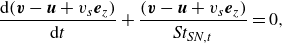(4.3) \begin{equation} \frac {\mathrm{d} (\boldsymbol{v}-\boldsymbol{u}+v_{s}\boldsymbol{e}_z)}{\mathrm{d}t} + \frac {(\boldsymbol{v}-\boldsymbol{u}+v_{s}\boldsymbol{e}_z)}{{\textit{St}}_{\textit{SN},t}}=0, \end{equation}

where we have used $\mathrm{d}v_{s}/\mathrm{d}t =0$ . The solution is given by

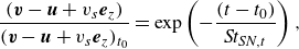(4.4) \begin{equation} \frac {(\boldsymbol{v}-\boldsymbol{u}+v_{s}\boldsymbol{e}_z)}{(\boldsymbol{v}-\boldsymbol{u}+v_{s}\boldsymbol{e}_z)_{t_0}} = \exp \left (-\frac {(t-t_0)}{{\textit{St}}_{\textit{SN},t}}\right ), \end{equation}

which shows that the particle slip velocities approach the kinematic model with an exponential decay with a dimensionless time scale given by ${\textit{St}}_{\textit{SN},t}$ , with an ‘initial condition’ $(\boldsymbol{v}-\boldsymbol{u}+v_{s}\boldsymbol{e}_z)_{t_0}$ at $t=t_0$ . At $(t-t_0) \gg {\textit{St}}_{\textit{SN},t}$ , we recover the kinematic model $\boldsymbol{v} = \boldsymbol{u} - v_{s}\boldsymbol{e}_z$ .

Figure 8 shows how the data compare against (4.4) during the particles’ approach to the kinematic model. We have to select the ‘initial time’ $t_0$ in (4.4) with care since the noise in the data is amplified when $(\boldsymbol{v}-\boldsymbol{u}+v_{s}\boldsymbol{e}_z)_{t_0}$ is small, and the particle release mechanism will impart some unknown initial motion to the particle. In the horizontal direction, we select $t_{x0}$ as the time when the horizontal slip velocity reaches its peak (see figure 7 a), after which it decays towards zero. For trajectories where the horizontal slip velocity does not have a clear peak, $t_{x0}$ is chosen as the time when $|(v-u)_x|$ begins to be smaller than $0.15 v_s$ . In the vertical direction, $t_{z0}$ is defined as the time when $|(v-u)_z|$ exceeds $0.7 v_s$ , by which time ${\textit{St}}_{\textit{SN}}$ is also within 20 % of ${\textit{St}}_{\textit{SN},t}$ .

Overall, the data show a reasonable agreement with the prediction in the horizontal direction, while it appears that the approach to the kinematic model in the vertical direction takes longer than predicted. The slower approach to the kinematic model in the vertical could be due to the history force (ignored here), which has been shown in previous experiments to have this effect (Mordant & Pinton 2000). Additionally, we see that forces related to drag, buoyancy, added mass and fluid acceleration are all important in the approach to the kinematic model. This is different to the case for particles with ${\textit{St}} \ll 1$ , where the kinematic model results from the drag–buoyancy forces being dominant. Finally, the Stokes number is important only to describe the transient phase in approaching the kinematic model. After that, only ${\textit{S}v}$ influences the particle motion.

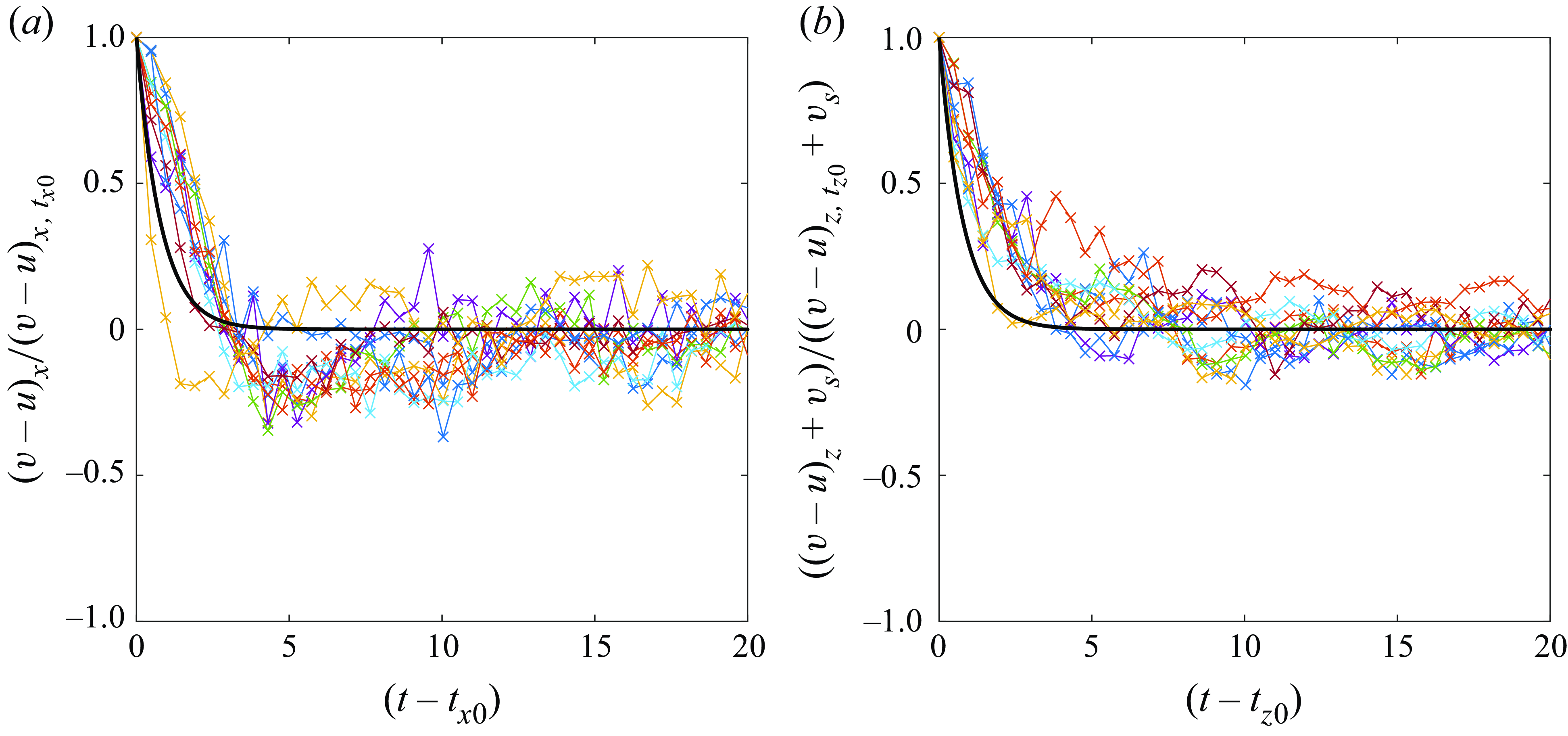
Figure 8. Evolution of $\boldsymbol{v}-\boldsymbol{u}+v_s \boldsymbol{e}_z$ for N1 particle data normalised by the initial condition in different directions: (a) horizontal, (b) vertical. Black solid lines are the analytical model (4.4).

4.1.2. Enhanced settling and dispersion

Since we found that ${\textit{St}}$ does not influence the particle motion after an initial transient phase, we can use the experimentally validated kinematic model (2.4) for particles below the $\textit{Ga}$ threshold for path instabilities to perform the same multiple time scale analysis as in DiBenedetto et al. (2022) to obtain the wave-averaged particle drift velocities. We find these (in dimensionless form) to be

(4.5) \begin{equation} v_{x\text{-}drift} = \frac {1}{1 + v_s^2} u_{{SD}}, \quad v_{z\text{-}drift} = -v_s\left [1 + \frac {1}{1 + v_s^2} u_{{SD}} \right ], \end{equation}

where $u_{{SD}} = \varepsilon _{w}^2 \cosh {2(Z_p +kh)}/2\cosh ^2kh$ is the classical dimensionless Stokes drift velocity with wave-averaged vertical particle position $Z_p$ , and $v_s$ is the dimensionless particle settling velocity, with all velocities made dimensionless using the wave speed $\omega /k$ . Equation (4.5) predicts that the horizontal drift is reduced while the vertical drift is enhanced, with both effects related to how the particle samples the fluid flow, and quantified by the term ${u_{{SD}}}(1/({1 + v_s^2}))$ . The settling velocity enhancement increases in percentage terms as the wave steepness increases and as the dimensionless particle settling velocity decreases.

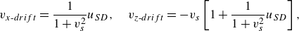
To check how well (4.5) predicts the settling velocity enhancement, we compute the net settling velocity using a single particle trajectory, following the double wave-averaging approach in DiBenedetto et al. (2022). Defining the wave average of quantity $s$ over wave period $T$ as $\overline {s} = ({1}/{T}) \int _{t}^{t+T} s(\tau )\,{\rm d}\tau$ , we wave average the particle vertical position and velocity once to remove the wave-induced oscillations, and once more to remove the influence of the initial wave phase at the release point. The double wave-averaged vertical velocity $\overline {\overline {v_z}}$ is then only a function of the double wave-averaged vertical position $\overline {\overline {z^{\prime}_p}}$ .

Figure 9. (a) Double wave-averaged velocity profiles of the N1 particles made dimensionless with the terminal settling velocity. Markers show data with 95 % confidence intervals, dashed lines show predicted enhanced settling (4.5), and vertical black dash-dotted lines indicate 95 % confidence interval of the terminal settling velocity (table 2). (b) Vertical profile of the standard deviation of the wave-averaged horizontal particle position for N1 particles.

Figure 9(a) shows profiles of $\overline {\overline {v_z}}$ as a function of $\overline {\overline {z^{\prime}_p}}$ for N1 particle data binned in vertical increments $0.1(z^{\prime}/h)$ and averaged across different particle releases. For $\overline {\overline {z^{\prime}_p}}/h\gt -0.3$ , the vertical drift is affected by the initial relaxation of the particle to the wave-induced flow, where its vertical slip velocity is smaller than the terminal settling velocity. Below this region, where the particle motion follows the kinematic model, the data appear to show a very small ( $1\,\%$ ) settling enhancement, which in turn is much greater than the enhancement predicted by (4.5) at these depths.

However, the settling enhancement suggested by the data should be interpreted with care since it falls within the uncertainty in the terminal settling velocity (dash-dotted lines). While (4.5) does not correctly predict the settling enhancement, it also does not account for the presence of Eulerian-mean flow. As seen in figure 2, although the Eulerian-mean flow is small compared to the wave-induced oscillatory flow, it is approximately $1\,\%$ of $v_s$ , and could be the cause of the settling enhancement in the data. We conclude that although a wave-induced settling enhancement cannot be ruled out, it is challenging to conclusively demonstrate it given the unavoidable sources of uncertainty and the smallness of the enhancement predicted from theory.

Apart from enhanced settling, DiBenedetto et al. (2022) also provided a discussion of the mechanisms by which inertial particles disperse in the horizontal direction while settling in waves. While no horizontal dispersion is predicted by divergence of the drift velocities (4.5), there is dispersion in the wave-resolved sense due to variations in the wave phase at the point of initial particle release. The variation in the initial phase can be understood as vertical variations in the effective wave-averaged initial positions, which are acted upon by the shear in the Stokes drift near the surface.

To quantitatively inspect the horizontal dispersion of the N1 particles, we compute the standard deviation of their wave-averaged horizontal positions. As the N1 particles undergo five wave periods while settling in the measurement area, we obtain their wave-averaged particle positions ( $\overline {x^{\prime}_p}$ and $\overline {z^{\prime}_p}$ ) for each wave period. The standard deviations of the horizontal particle positions with corresponding mean vertical positions are then determined by bootstrapping using data for each wave period. Note that since the particles are subjected to similar wave-induced flows, their vertical displacements are nearly uniform across the particles for each wave period, leading to negligible confidence intervals in $\overline {z^{\prime}_p}$ .

Figure 9(b) shows the vertical profile of the dimensionless standard deviations of the wave-averaged horizontal particle positions. While the standard deviation increases near the surface as particles with different initial wave phases spread out, it remains relatively constant in $\overline {z^{\prime}_p}/h\lt -0.2$ , which is consistent with the mechanism discussed in DiBenedetto et al. (2022). Note that the small changes in the standard deviation in $\overline {z^{\prime}_p}/h\lt -0.2$ could be due to the weak Eulerian-mean flows, and they are not investigated further.

4.2. Path instabilities

To understand why certain particles show large deviations from the kinematic model, we compared how spheres settle in waves with the corresponding data in quiescent water. Figure 10 shows images of particles N1 and N3 (smallest and largest $\textit{Ga}$ values, respectively) with black markings on them to visualise particle rotation. The markings on the N1 particle do not move, showing that the particle had little to no rotation, as expected for a particle settling in a quiescent fluid and an irrotational flow. However, the markings on the N3 particle change consistently, indicating that the particle rotates while settling in both quiescent fluid and in irrotational waves. Since there is no mechanism by which irrotational wavy flow can cause rotations of spherical particles, we conclude that the oscillations in horizontal slip velocity in wavy flow for our larger $\textit{Ga}$ particles must be due to path instabilities. In other words, the deviations of particle motion from the kinematic model are due to fluid inertia rather than particle inertia.

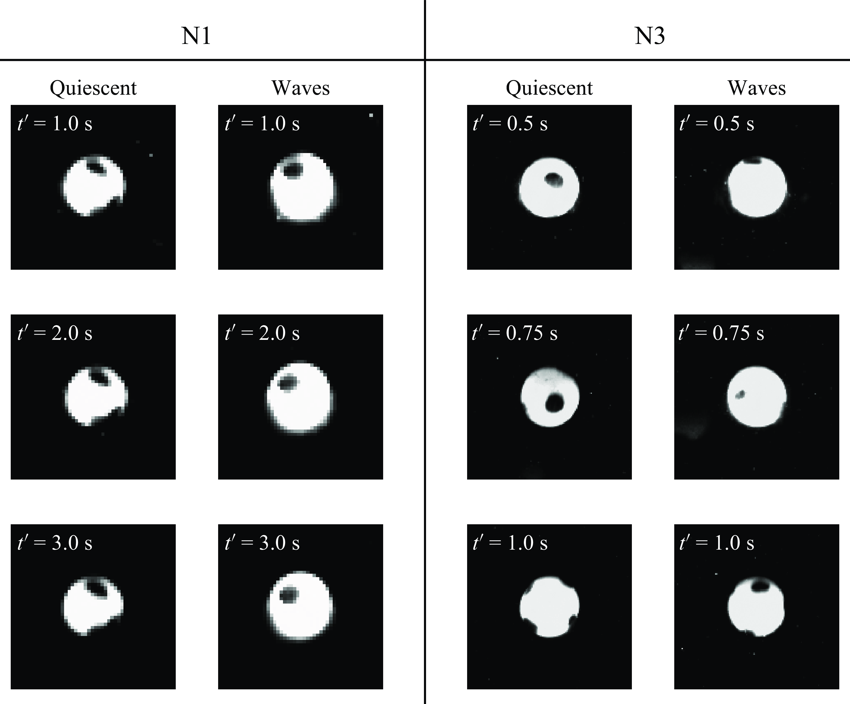
Figure 10. The N1 and N3 particles with surface markings settling in quiescent water and waves.

To explore the path instabilities more quantitatively, we calculated spectra of the particle slip velocity $P(f)$ , where $f$ is the frequency. Specifically, we used the dimensional slip velocity in waves $(\boldsymbol {v}^{\prime }-\boldsymbol {u}^{\prime })$ , and the dimensional particle velocity in quiescent conditions $\boldsymbol v^{\prime }$ . Note that by using the particle slip velocity, we avoid the spectral peak produced by the wave-induced oscillations in particle motion. We used the data over the vertical region $-0.8 \lt z^{\prime}/h \lt -0.3$ , where the vertical slip has already relaxed to the particle’s terminal settling velocity, but the particle motion is still affected by the wave-induced flow. To compute the spectra, we first matched the length of the slip velocity data time series for all data of a given particle in both waves and quiescent conditions by excluding the last few data points in order to ensure consistency in the frequency resolution. Typically, no more than three data points were excluded. We also subtracted the mean from the time series of each particle release to obtain time series of zero-mean velocity fluctuations (slip velocity in waves $(\boldsymbol {v}^{\prime }-\boldsymbol {u}^{\prime })^*$ and particle velocity in quiescent conditions $(\boldsymbol{v}^{\prime })^*$ ). The spectrum for each particle release was then computed using the fast Fourier transform on the zero-mean time series before being ensemble averaged across different particle releases (as recommended in Bendat & Piersol 2011). Finally, the ensemble mean spectrum and its confidence interval at each frequency were determined via bootstrapping across the spectra.

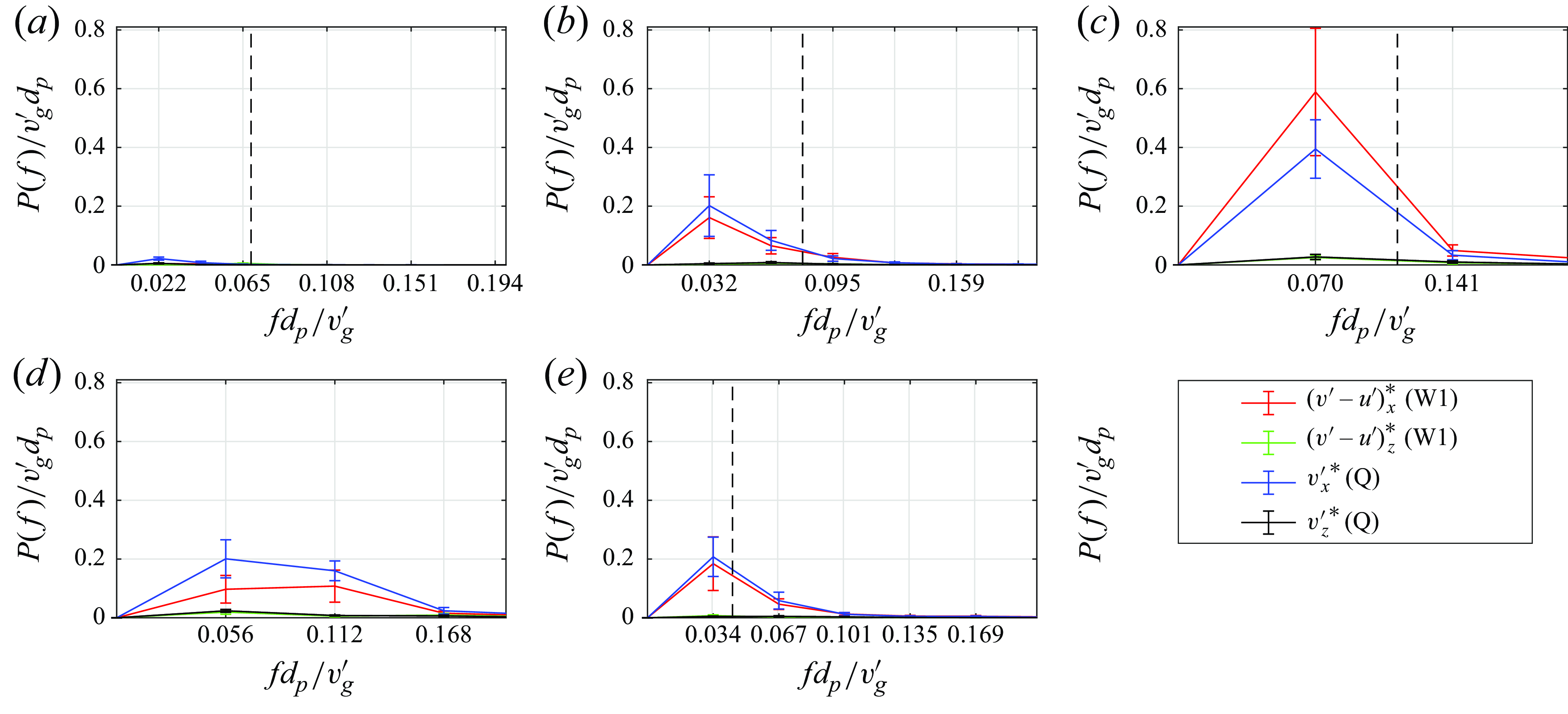
Figure 11. Normalised ensemble mean spectra of particle slip velocity fluctuations in waves and quiescent fluid for (a) N1, (b) N2, (c) N3, (d) N4, (e) T1. Vertical dashed lines indicate the dimensionless wave frequency ( $d_p/Tv^{\prime}_g$ ), with $d_p/Tv^{\prime}_g \approx 0.22$ in (d) not shown.

Figure 11 shows the ensemble mean spectra for each particle type using 10 particle releases in both quiescent fluid and waves. While the spectra for the N1 particle ( ${\textit{Ga}} = 126$ , below the ${\textit{Ga}} \approx 155$ threshold for path instabilities) show no peaks, the spectra of the other particles show clear peaks with magnitudes 1–2 decades larger in the horizontal direction compared to the vertical. The normalised frequencies at which the spectral peaks occur in our data agree with previously reported values for similar $\textit{Ga}$ - and $\gamma$ -valued particles settling in quiescent conditions (Veldhuis & Biesheuvel 2007; Raaghav et al. 2022; Cabrera-Booman et al. 2024). Since the wake instabilities of spheres settling in quiescent fluid are determined solely by particle and fluid properties, the spectral peaks occur at the same frequencies regardless of whether the particles are settling in quiescent fluid or in waves, and these frequencies are distinct from the wave frequency, we conclude that the deviations from the wave-induced flow in the horizontal direction (figure 7) are indeed due to asymmetric wakes and path instabilities, and that these path instabilities are unaffected by the waves. Note that the lack of influence of the oscillatory wave-induced flow on the path instabilities caused by particle wakes is different to, for example, the case where spheres or cylinders are forced to oscillate transversely across a free stream flow (Williamson & Roshko 1988; Peter & De 2016), in which the wake vortex frequency is influenced by the forced oscillation frequency.

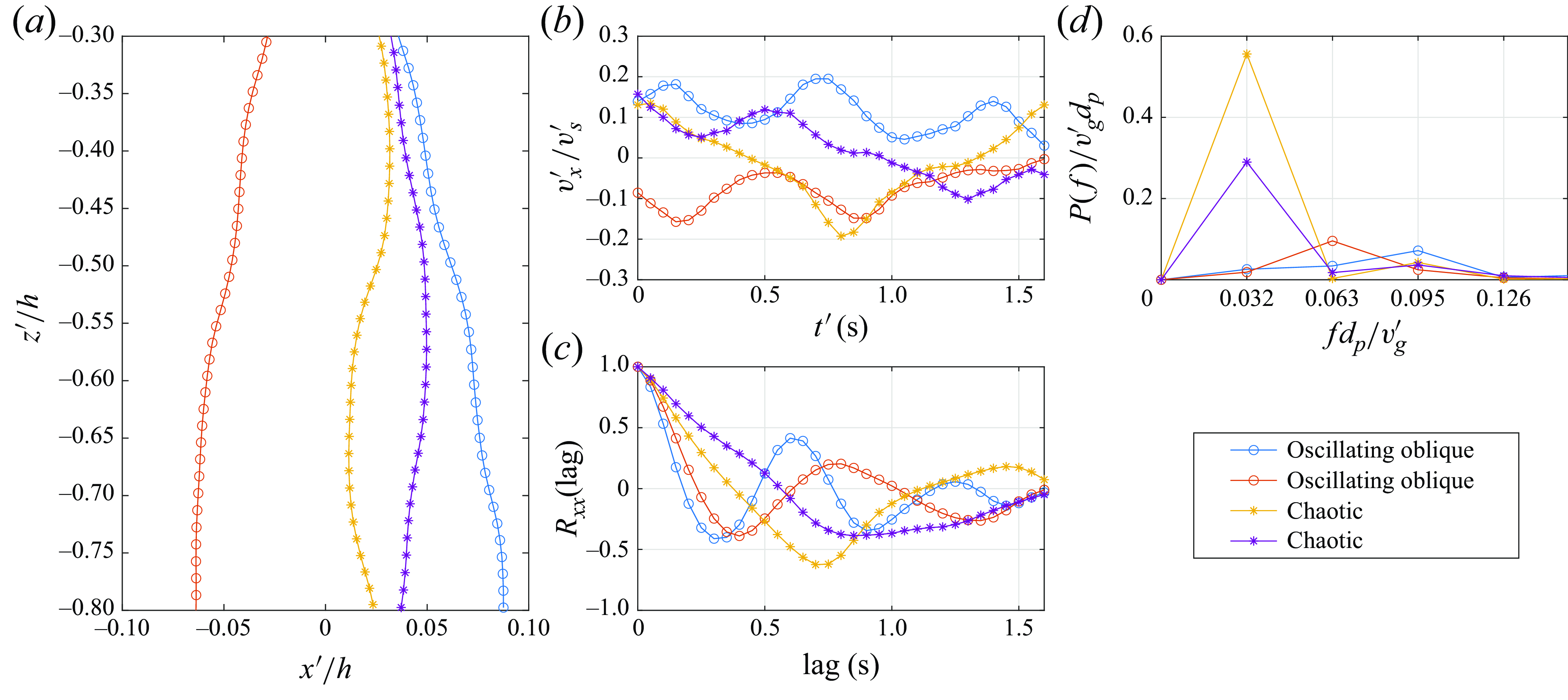
Figure 12. The N2 particles settling in quiescent fluid: (a) example trajectories; (b) normalised horizontal particle velocities; (c) horizontal particle velocity autocorrelation function; (d) normalised spectra of horizontal particle velocities.

While the data in figure 11 suggest that the wave-induced flow has little influence on the particle path instabilities, the spectral peaks are broad and the frequency resolution is coarse. Furthermore, the data are from a single wave case, leaving open the question of whether the waves might affect the path instabilities at different wave frequencies. We address these points using N2 particle data spanning wave cases W1, W2 and W3 (§ 3.2.2) and further analysis.

Figure 12 shows further analysis of N2 particles settling in quiescent fluid. In the example trajectories in figure 12(a), we observe two distinct regimes of path instabilities: a low-frequency oscillating oblique regime (circles), and a chaotic regime (asterisks). This is not surprising since N2 particles are at the boundary between the two different regimes in $\textit{Ga}$ – $\gamma$ space (see figure 5 in Raaghav et al. 2022), and the particle properties have small variations across different particles of each type. In the oscillating oblique regime, there are multiple oscillations, but the sign of the horizontal velocity remains unchanged, resulting in a non-negligible mean (figure 12 b). In contrast, in the chaotic regime, there is one or fewer oscillations, but they occur around a near-zero mean horizontal velocity with a change in sign (figure 12 b). These differences are reflected in the horizontal velocity autocorrelations ( $R_{xx} ({\text{lag}}) = \langle v^{\prime *}_x(t^{\prime})\, v^{\prime *}_x(t^{\prime}+{\text{lag}})\rangle /\langle (v^{\prime *}_x)^2\rangle$ , where $\langle \boldsymbol{\cdot} \rangle$ denotes a mean over the time series; see figure 12 c), which show a distinct peak for the oscillating oblique regime, and no distinct peak for the chaotic regime. The horizontal velocity spectra (figure 12 d) show that the peaks for the two regimes are at different frequencies. While the spectral peaks for the oscillating oblique regime occur at frequencies corresponding to the lags associated with the peaks in the autocorrelation functions ( $\approx 0.6$ and $0.8$ s), the spectral peaks for the chaotic regime occur at the smallest resolved frequency (i.e. the first non-zero bin) since the trajectories are too short to observe complete oscillations. We also note that the variance of the horizontal particle velocity for the oscillating oblique regime is much smaller than that for the chaotic regime, which results in a smaller spectral peak.

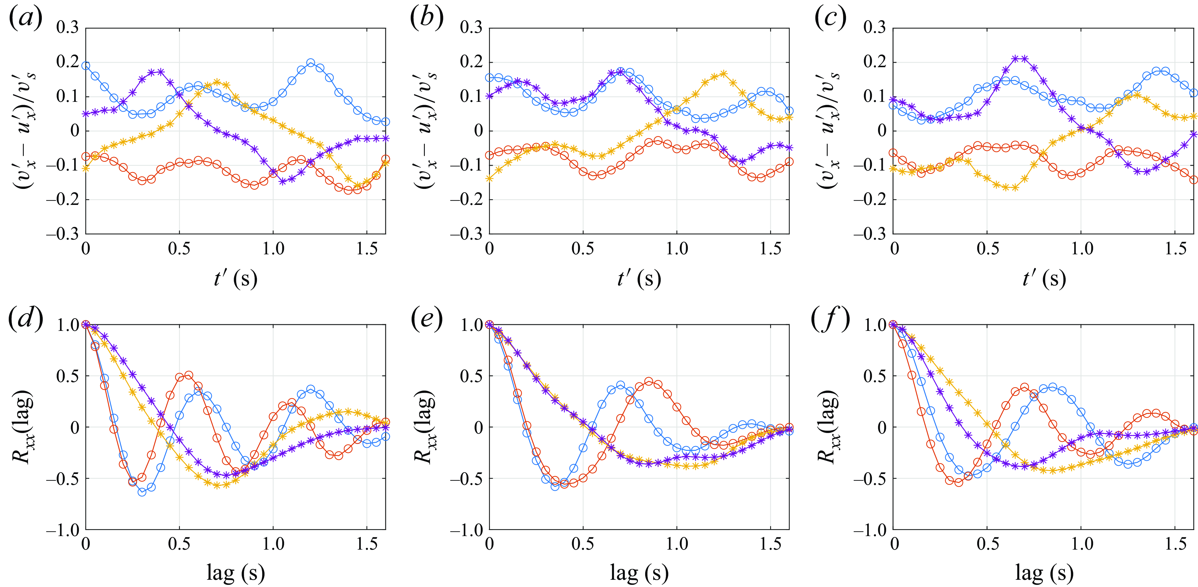
Figure 13. The N2 particles settling in waves. Examples of normalised horizontal slip velocities and the corresponding horizontal slip velocity autocorrelation functions for different wave cases: (a,d) W1, (b,e) W2, (c,f) W3.

Figure 13 shows the corresponding analysis for N2 particles settling in waves. The wave-induced oscillatory motion of particles makes it difficult to identify different path instability regimes from particle trajectories, but we find that the horizontal slip velocities show features that resemble the same two different regimes: a low-frequency oscillating oblique regime (circles), and a chaotic regime (asterisks) (figure 13 a–c). As in the data from quiescent fluid, there are multiple oscillations with the same sign for the oscillating oblique regime, whereas there are one or fewer oscillations with a change in sign in the chaotic regime. The corresponding slip velocity autocorrelation functions (figure 13 d–f) show distinct peaks for the former, while no distinct peak is observed for the latter, just as in the quiescent fluid case.

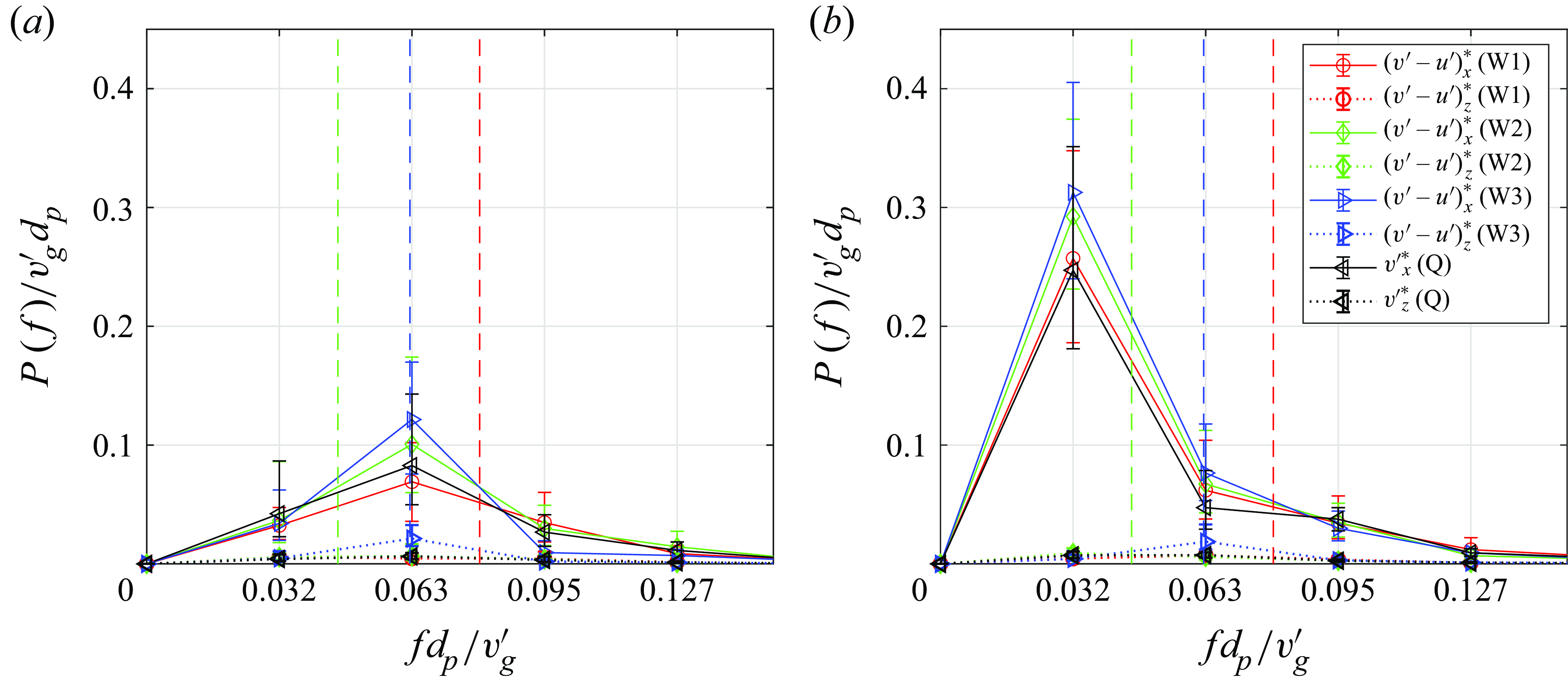
Figure 14. Normalised ensemble mean spectra of N2 particle slip velocity fluctuations in waves and quiescent fluid: (a) oscillating oblique regime; (b) chaotic regime. Vertical dashed lines indicate the dimensionless wave frequency ( $d_p/Tv^{\prime}_g$ ), with different colours corresponding to different wave cases.

With the knowledge of the two different path instability regimes, we can return to the comparison between the spectra in quiescent fluid and in waves presented in figure 11, and use the N2 particle data to confirm that the magnitude and width of the spectral peaks are unaffected by the waves. Figure 14 shows the ensemble mean spectra split into the low-frequency oscillating oblique regime and the chaotic regime. Each spectrum comes from the mean of approximately 12 particle releases (from a total of 25 releases, with both regimes being equally likely), and the particle in each release experiences a significant wave-induced flow for at least one wave period while settling through the region of analysis ( $-0.8 \lt z^{\prime}/h \lt -0.3$ ). We note that while the coarse frequency resolution is a fundamental limitation of the short particle trajectories (see also Veldhuis & Biesheuvel 2007; Cabrera-Booman et al. 2024), which themselves are limited by the finite depth of the wave-influenced region, the time domain analysis in figures 12 and 13 confirms the robustness of the spectral peaks.

We observe that in both path instability regimes, the presence of the waves does not affect either the magnitude or the width of the spectral peak in figure 14. This is true across the three different wave cases with different frequencies, where $T/T_{\textit{oscillating oblique}} = 0.80, 1.4, 1.0$ and $T/T_{\textit{chaotic}} = 0.40, 0.70, 0.51$ , with $T_{\textit{oscillating oblique}}$ and $T_{\textit{chaotic}}$ being the periods associated with spectral peaks for the two path instability regimes, and $T$ being the wave period. Moreover, the spectral peaks occur at dimensionless frequencies that are distinct from those associated with the wave period. These results demonstrate that path instabilities of settling particles observed in quiescent fluid persist in the unsteady wave-induced flows, and account for the deviation of particle velocities from the kinematic model. We suspect that the lack of interaction between the particle wakes and the wavy flow is due to the smallness of ${\textit{Sz}}$ (table 3), which implies a large-scale separation between the particles and the flow length scale.

5. Conclusions

We have investigated the effects of particle and fluid inertia on the dynamics of spherical particles settling in the two-dimensional, non-uniform, unsteady and irrotational flow induced by surface waves. The particles are small ( ${\textit{Sz}}\lt 0.06$ ) and weakly negatively buoyant ( $(\gamma - 1) \lt 0.4$ , $(1 - \beta) \lt 0.21$ ), are inertial from both the particle perspective ( ${\textit{St}}=O(1)$ ) and the fluid perspective ( $125 \lt {\textit{Ga}} \lt 550$ , corresponding to $100 \lt {\textit {Re}}_{p,t} \lt 1000$ ), and settle over a range of velocities relative to the fluid velocity ( $0.8 \leqslant Sv \leqslant 2.4$ ). By capturing the motion of the particle and tracers simultaneously using a single camera, particle velocities and flow velocity fields are estimated via particle tracking and particle image velocimetry, respectively, with the latter used to estimate the undisturbed flow velocity at the particle position.

We observed that particle motion is well described by the simple kinematic model $\boldsymbol{v}=\boldsymbol{u}-v_s\boldsymbol{e}_z$ after a transient period, as long as the effects of fluid inertia are small enough that they do not induce path instabilities. To rationalise this observation, we show how an ad hoc Maxey–Riley–Gatignol (MRG) equation, where the Stokes drag is replaced with the drag force from the Schiller–Naumann drag correlation, can be simplified to show that particle dynamics will approach the kinematic model. In this analysis, we find that all terms in the MRG equation (particle acceleration, drag, buoyancy, fluid forcing, and added mass) are important. Additionally, while ${\textit{St}}$ is important to predict the time scale over which the particle dynamics approach the kinematic model, only ${\textit{S}v}$ is required to predict particle motion once the particle motion is well described by the kinematic model. Thus, although ad hoc extensions of the MRG equation have been developed to extend its applicability to large particle Reynolds number, the motion of settling particles with significant particle and fluid inertia is actually better described by the simple kinematic model $\boldsymbol{v}=\boldsymbol{u}-v_s\boldsymbol{e}_z$ .

For particles that follow the kinematic model, we give the wave-averaged particle drifts. While the data show qualitative agreement with the mechanism for horizontal dispersion from DiBenedetto et al. (2022), we find that the settling velocity enhancement, if it exists, is too small to be measurable within experimental uncertainties.

As fluid inertia increases ( ${\textit{Ga}} \gtrsim 155$ , corresponding to ${\textit {Re}}_{p,t} \gtrsim 210$ ), we observed path instabilities in particle trajectories. By examining the similarities in the horizontal velocity of settling particles in quiescent fluid, and the horizontal slip velocity of settling particles in waves, along with their autocorrelation and spectra, we confirmed that these path instabilities are caused by wake effects that have been reported previously to occur for settling particles in quiescent fluid. Remarkably, these path instabilities appear to be unaffected by the background flow even when ${\textit{St}} =O(1)$ , ${\textit{S}v} = O(1)$ , and the ratios between the wave period and dominant path instability period are below, at and above unity. Thus, we conclude that this lack of interaction between the background flow and the particle wakes is because ${\textit{Sz}} \ll 1$ , meaning that there is a large separation between the particle size and the length scale of the flow.

For applications of inertial particle settling in non-trivial flow environments, future studies should focus on the role of fluid inertia (as well as particle inertia) as even small, weakly negatively buoyant particles ( $\gamma \approx 1.1$ , $d_p \approx 3$ mm particles in water) can be expected to have path instabilities. Similarly, other particle types, such as positively buoyant particles, bubbles, and particles with complex shapes, will have their own regimes of path instabilities. While we have found wave-induced flow (two-dimensional, unsteady and non-uniform) to be an attractive testing ground to understand flow–particle interactions that is also relevant to environmental and geophysical applications, it is difficult to extrapolate our findings directly to more complex flows since wavy flow is irrotational and varies over a single length and time scale. Thus, it would also be interesting to understand to what degree the current results hold or are modified in multi-scale flow environments (e.g. turbulence).