Generalized Lagrangian heterogeneous multiscale modelling of complex fluids

Abstract

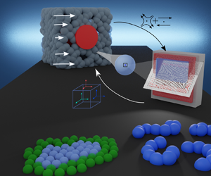
We introduce a fully Lagrangian heterogeneous multiscale method (LHMM) to model complex fluids with microscopic features that can extend over large spatio/temporal scales, such as polymeric solutions and multiphasic systems. The proposed approach discretizes the fluctuating Navier–Stokes equations in a particle-based setting using smoothed dissipative particle dynamics (SDPD). This multiscale method uses microscopic information derived on-the-fly to provide the stress tensor of the momentum balance in a macroscale problem, therefore bypassing the need for approximate constitutive relations for the stress. We exploit the intrinsic multiscale features of SDPD to account for thermal fluctuations as the characteristic size of the discretizing particles decreases. We validate the LHMM using different flow configurations (reverse Poiseuille flow, flow passing a cylinder array and flow around a square cavity) and fluid (Newtonian and non-Newtonian). We show the framework's flexibility to model complex fluids at the microscale using multiphase and polymeric systems. We also show that stresses are adequately captured and passed from micro to macro scales, leading to richer fluid response at the continuum. In general, the proposed methodology provides a natural link between variations at a macroscale, whereas accounting for memory effects of microscales.

1. Introduction

The modelling of complex fluids, synthetic or biological, is in general a challenging task due to the multiscale nature of the flow, leading to complex behaviours such as flow-induced phase separation, shear-thinning/thickening and viscoelasticity. Usual approaches involve the solution of a macroscopic balance of momentum, along with constitutive equations that relate the dependency of the stresses and velocity fields due to microscopically originated features. However, limitations of these approaches arise when the constitutive equations are not known a priori. Moreover, the existence of large relaxation times at the microscale results in a non-trivial interplay with macroscopic flow features, requiring a detailed description of the entire stress history. In this context, heterogeneous multiscale methods (HMMs) (Ee et al. 2007) that combine numerical algorithms to resolve separately macro- and microscales, appear as powerful tools to model the behaviour of fluids across scales. In HMMs, microscales are localized and solved on parts of the domain to obtain microscopically derived properties that are used to close the macroscale problem (Ren & Weinan 2005). This methodology offers the advantage of capturing microscopic effects at the macroscopic length scales, with a lower cost than solving the full microscale problem in the whole domain. In HMMs, the derived microscales properties can enter into the macroscales representations either through constitutive relationships or microscopic stresses information without a priori assumption of the constitutive relationships. The latest is an important advantage of HMMs for the modelling of complex fluids. For an extended review on HMMs, the reader is referred to the work of Ee et al. (2007). One of the key benefits of having a constitutive equation for stress is the ability to generalize fluid behaviour in the macroscopic domain without the need for explicit microscopic simulations. Such constitutive relations have been formulated for various non-Newtonian fluids (Bird et al. 1987). However, many complex systems lack an a priori constitutive relationship, which necessitates system-specific approximations. In this context, using microscopically informed stress for the momentum equation provides a more systematic approach to bypass the need for unknown constitutive models. The primary assumption with this strategy is that the adopted methodology used for the microscales should be capable of reproducing the physical system. Consequently, the microscales will typically require preliminary characterization.

Depending on the type of discretization (Eulerian or Lagrangian) used for macro- and microscales, the HMMs are classified as Eulerian/Eulerian (EE), Lagrangian/Lagrangian (LL), Eulerian/Lagrangian (EL) and Lagrangian/Eulerian (LE); see figure 1(a). A large part of the existent HMMs relies on EE and EL schemes (Ee et al. 2007), where the macroscale dynamics is resolved on a fixed grid (using a variety of methods such as finite elements, finite volumes, lattice Boltzmann, to name a few), and microscale simulations (e.g. molecular dynamics (Alexiadis et al. 2013; Borg, Lockerby & Reese 2015; Tedeschi et al. 2021), coarse-graining methods, stochastic methods, etc.) are associated with grid points, where microscopic properties are derived. For viscoelastic fluids modelling, Laso and Öttinger introduced a pioneering approach known as CONNFFESSIT (Laso & Öttinger 1993) (calculation of non-Newtonian flow: finite element and stochastic simulation technique), combining finite elements at the macroscale and stochastic particle simulations of polymer dynamics at the microscale.

Figure 1. Scheme of different HMM approaches. Eulerian–Eulerian (EE), Eulerian–Lagrangian (EL) and Lagrangian–Lagrangian (LL). The evolution of the stress tensor depends on the effective relaxation times at the microscales $\lambda '$. Systems with $\lambda ' \ll \bar {\lambda }$ (green) are accurately computed at the microscopic scales, whereas for $\lambda ' \leq \bar {\lambda }$ (blue), larger microscale simulations are required to capture memory effects as the macro scales evolve. LL approaches facilitate the carrying of the stress information during the time integration at macroscales.

The EE and EL approaches are generally appropriate for fluids with microstructural relaxation times (${\lambda }'$) that are sufficiently small compared to the macroscopic ones (${\lambda }$) (Ren & Weinan 2005; Yasuda & Yamamoto 2008, 2014). As shown in figure 1(b), for multiscale problems with significant time scale separation, where ${\lambda }' \ll {\lambda }$ (or $Wi = {\lambda }'/ {\lambda } \ll 1$, where $Wi$ is the Weissenberg number), a quasi-steady state can be achieved for the microscopic stresses, regardless of the flow history. This approach has been employed in atomistic-continuum simulations of simple fluids using molecular dynamics with an Eulerian grid-based calculation of the flow field (Ren & Weinan 2005). In simple fluids, the local stress depends point-wise in time on the velocity gradient, and therefore, the initial conditions for the microstructure can be chosen arbitrarily at each time step. The average stress is then calculated using the Irving–Kirkwood approximation, provided that local stationarity is achieved within the same time step.

However, this approach cannot be extended to complex fluids with finite memory, when ${\lambda } \lesssim {\lambda }'$ ($Wi>1$). As shown in figure 1(b), the stresses and microstructure heavily depend on flow history, and relaxation times are likely to be comparable to, or even exceed, the macroscopic time step. The direct use of EL or EE schemes to generate an initial microstructural configuration in a fixed fluid cell is fundamentally and technically limited due to two reasons. First, it is not known beforehand where the fluid comes from and what its flow history was, and second, even if this information were available, it would require additional constitutive and numerical features capable of accounting for complex spatio/temporal variations.

Alternative techniques to address these issues include spatial/temporal homogenization methods and backward-tracking Lagrangian particles combined with Eulerian grids to capture memory effects in the fluid (Phillips & Williams 1999; Wapperom, Keunings & Legat 2000; Ingelsten et al. 2021). However, fluid memory can be very long in polymer systems, suspensions, etc., precluding simple linear backward approximations. Regarding the second issue, one alternative is to incorporate continuum configuration fields that can be discretized and advected from the macroscales (Ottinger, van den Brule & Hulsen 1997). However, it would be extremely challenging to know a priori those fields for general multiphysics problems (i.e. non-polymeric), as well as the numerical generation of microscopic configurations consistent with the history of the fluid.

For systems with larger microstructural relaxation times (${\lambda } \lesssim {\lambda }'$), the particular restrictions of EE and EL can be circumvented using fully Lagrangian, LL, schemes (Ee et al. 2007), and a proper sampling procedure for the microstructure. Indeed, LL schemes have been successfully used to model elastic effect and history-dependent flows (Murashima & Taniguchi 2010; Seryo et al. 2020; Morii & Kawakatsu 2021) at large Weissenberg numbers. As illustrated in figure 1(b), LL schemes directly track the material points at the macroscale retaining their strain and strain-rate variation, thus naturally handling history-dependent fluids. A variety of LL methodologies have emerged over the last decade, adopting mainly smoothed particle hydrodynamics (SPH) discretizations at the macroscales and combination of different microscopic models (Ellero, Español & Flekkoy 2003; Murashima & Taniguchi 2010; Feng et al. 2016; Xu & Yu 2016; Sato & Taniguchi 2017; Zhao et al. 2018; Sato, Harada & Taniguchi 2019; Giessen et al. 2020; Schieber & Hütter 2020; Seryo et al. 2020; Morii & Kawakatsu 2021). At the microscales, the stress evolution of polymeric solutions and entanglements have been accounted for using Brownian dynamic (Xu & Yu 2016), active learning (Zhao et al. 2018; Seryo et al. 2020) and slip-link models (Feng et al. 2016; Sato & Taniguchi 2017; Sato et al. 2019). In these LL schemes, it is considered that microscales only account for the polymer contribution to the stress, whereas the fluid is modelled uniquely from the macroscopic discretization (Feng et al. 2016). Its effect (i.e. velocity gradient tensor) enters the Langevin-type dynamics for stochastic micro-realizations implicitly as a single parameter, and not directly as a boundary condition for the full microsystem.

In fact, one important issue limiting the applicability of HMM methods to more detailed descriptions of complex fluids is precisely the proper imposition of microscale constraints that are consistent with the macroscale kinematics and the calculation of microscopic information required by the macro state (Ee et al. 2007). When using particle-based micro-models with explicit solvent description (e.g. molecular dynamics, dissipative particle dynamics, discrete element method, SDPD), the construction of this constrained microscale solver represents often the most cumbersome technical step. For LL schemes, due to the history-dependent evolution of the flow and the existence of non-trivial flow configurations, the microscales can be subjected to arbitrary series of deformations that are usually difficult to handle with traditional periodic boundary conditions (BCs). To avoid these limitations, existent LL schemes have been restricted to the use of microscopic simulators that do not depend on the ‘physical’ boundary conditions (Feng et al. 2016; Sato & Taniguchi 2017; Sato et al. 2019; Morii & Kawakatsu 2021). This includes, for example, the case of Brownian dynamics for statistically independent polymers, such as dilute polymer solutions or polymer melts in mean field approximation, or where geometries that reproduce simple flow configurations are utilized (Seryo et al. 2020) (i.e. simple shear or uniaxial deformation). More general micro–macro couplings (e.g. full particle-based model of polymeric dispersions, colloid suspensions, emulsions, etc.) involving detailed microsystems models undergoing arbitrary flow deformations are beyond the capabilities of the current frameworks.

Another important assumption in some of the existent microsolvers is that the microscopic states of all polymers are in equilibrium and that the coils do not have translational degrees of freedom, but only rotational and extensional ones (Morii & Kawakatsu 2021). Regarding microscopic BCs approaches using simple flow configurations, they are suitable to account for translational effects and often provide information sufficient to characterize simple fluids. However, since complex fluids can possess microscopic structures that are influenced by different flow configurations, geometries, time scales and deformation rates, it has been evidenced that to correctly model non-Newtonian fluids (Tedeschi et al. 2021), it is necessary to determine the full stress contribution from the microscopic solver.

In this manuscript, we propose a generalized fully Lagrangian HMM (LHMM) using smoothed dissipative particle dynamics (Español & Revenga 2003; Ellero & Español 2018) (SDPD), suitable to model general complex fluids (e.g. colloids, polymer, microstructures in suspensions) while using the same fluid description across scales. Among the different computational methods successfully used to model Newtonian and non-Newtonian fluids at continuum and microscales, SDPD has emerged as a suitable tool to simulate complex fluids (Kulkarni et al. 2013; Müller, Fedosov & Gompper 2014; Ellero & Español 2018). The main strengths of SDPD are: (i) it consistently discretizes the fluctuating Navier–Stokes equations allowing the direct specification of transport properties such as viscosity of the fluid; (ii) SDPD is compliant with the general equation for non-equilibrium reversible–irreversible coupling (GENERIC) (Öttinger 2005) and therefore, it discretely satisfies the first and second laws of thermodynamics, and fluctuation–dissipation theorem (FDT); (iii) at macroscopic scales, SDPD converges to the well-known continuum method smoothed particle hydrodynamics (SPH) as the characteristic size of the discretized particle increases (Vázquez-Quesada, Ellero & Español 2009; Ellero & Español 2018). For an extended review of SDPD, the reader is referred to the publication of Ellero & Español (2018).

Since SDPD offers a natural physical link between different scales, we construct an HMM that uses SDPD to solve both macro- and microscales. This approach ensures the compatibility of the different representations by construction and physical consistency across scales. At the microscales, we adopt the recently proposed BC methodology (Moreno & Ellero 2021) that allows the acquisition of the full microscopic stress contributions for arbitrary flow configurations. This allows to carry out micro-computations under general mixed flow conditions. While it is true that CONNFFESSIT (Laso & Öttinger 1993) and other EL methodologies are also capable of handling mixed flow features, those features are not included in current LL methodologies with fully explicit solvent descriptions. Furthermore, in the context of LL, our approach exploits the versatility of SDPD to model a variety of microscopic physical systems beyond polymeric systems. Our LHMM scheme's strength lies in its unique combination of aspects that other methods only partially account for. We can summarize the main features of the proposed LHHM framework as follows.

1. (i) Model history-dependent flows by construction.

2. (ii) Significant spatio-temporal gains in simulations compared with fully resolved microscale simulations.

3. (iii) Thermodynamic-consistent discretization of the fluctuating Navier–Stokes equations in both macro- and microscales (deterministic–stochastic) providing a direct link to physical parameters.

4. (iv) GENERIC compliant at both macro and micro levels.

5. (v) Multiphysics – polymers, colloids, suspensions, multiphasic systems. No constitutive models for closure are required.

6. (vi) Complex-flow configurations are allowed and can be handled at the microscales.

In the following sections, first, a general description of HMM is introduced along with the governing balance equations, then, the proposed fully Lagrangian approach and the particle-based discretization are presented. Finally, without loss of generality, we streamline the validation of the methodology focusing on two-dimensional simulations of complex flows with memory. At the microscales, we adopt generic, yet complex, polymeric and multiphase flows to showcase the flexibility of the method.

2. Heterogeneous multiscale methods

In general, for HMMs, we can define the macroscopic problem considering a domain $\varOmega \subset \mathcal {R}^D$ (with dimension $D=2,3$) with a boundary $\partial \varOmega = \varGamma _{\mathcal {D}} \cup \varGamma _{\mathcal {N}}$, where $\varGamma _{\mathcal {D}}$ and $\varGamma _{\mathcal {N}}$ correspond to boundary regions where Dirichlet and Neumann boundary conditions are applied, respectively. The mass and momentum balance of the system for an incompressible fluid with constant density $\rho$ can be expressed as

(2.1)\begin{equation} \left. \begin{aligned} \boldsymbol{\nabla} \boldsymbol{\cdot} {\boldsymbol{v}} & = 0, \quad \text{in} \ \varOmega \times (0,T),\\ \rho \frac{\text{d} {\boldsymbol{v}}}{\text{d} t} - \boldsymbol{\nabla} \boldsymbol{\cdot} \boldsymbol\tau({\boldsymbol{v}},p) & = f ,\quad \text{in} \ \varOmega \times (0,T),\\ {\boldsymbol{v}} & = g, \quad \text{on} \ \varGamma_{\mathcal{D}} \times (0,T), \\ {\boldsymbol{v}}(0) & = {\boldsymbol{v}}_0, \quad \text{in} \ \varOmega \times \{0\}, \end{aligned} \right\} \end{equation}

where the total stress tensor is given by ${\boldsymbol \tau } = -p{\boldsymbol I} + \boldsymbol {\pi }$, with $p$ being the pressure and $\boldsymbol {\pi }$ the viscous stress. For incompressible Newtonian fluids, the viscous stress is a linear function of the strain rate ($\boldsymbol {\pi }=\eta (\boldsymbol {\nabla }{\boldsymbol v} + \boldsymbol {\nabla }{\boldsymbol v}^T)$, with $\eta$ being the viscosity) and the flow can be totally described using (2.1). For non-Newtonian fluids such as colloidal and polymeric systems, this linear behaviour does not hold and other relationships are required (Bird et al. 1987). Additionally, for microfluidics, where complex flow patterns and thermal effects may arise, the use of Dirichlet boundary conditions, ${\boldsymbol {v}} = g$ on $\varGamma _{\mathcal {D}} \times (0,T)$, may not accurately model such microscopic effects, requiring more elaborated considerations for the boundary conditions.

2.1. Lagrangian heterogeneous multiscale method (LHMM)

We propose an LL-type of methodology, as depicted in figure 1, discretizing both macro- and microscales with a particle-based representation of the system. We distinguish macroscale parameters and variables if they are derived from microscales calculations using the upper bar (i.e. $\bar {X}$), whereas microscale variables are denoted using a prime (i.e. $X'$). We use the subindices $x,y$ and $z$ to indicate the coordinate axis. If we express the macroscopic viscous stress determined from a representative microscopic domain $\varOmega '$ in terms of hydrodynamic, non-hydrodynamic and kinetic contributions as ${\bar {\boldsymbol {\pi }}}={\bar {\boldsymbol {\pi }}}_{h}+{\bar {\boldsymbol {\pi }}}_{m}+{\bar {\boldsymbol {\pi }}}_{k}$, the ensemble average stress at the microscales leads to

(2.2)\begin{align} \langle \bar{\boldsymbol{\pi}} \rangle (\boldsymbol x) &= \frac{1}{\varOmega'} \int_{\varOmega'}{\boldsymbol{\pi}'} \,\text{d} \varOmega', \nonumber\\ &= \frac{1}{\varOmega'} \left(\int_{\varOmega'} {\boldsymbol{\pi}}_h' \,\text{d} \varOmega' + \int_{\varOmega'} {\boldsymbol{\pi}}_m' \,\text{d} \varOmega' + \int_{\varOmega'} {\boldsymbol{\pi}}_k' \,\text{d} \varOmega' \right), \end{align}

where ${\boldsymbol {\pi }}_h'$ accounts for the hydrodynamic contributions to the stress and ${\boldsymbol {\pi }}_m'$ corresponds to the non-hydrodynamics effects (presence of colloids, polymers, walls, etc). The $\langle \boldsymbol {\cdot }\rangle$ denotes the averaging over the microscopic domain. However, the $\bar {\boldsymbol {\pi }}$ corresponds to a macroscopic field. For a Newtonian (ideal) solvent, the stress is given by $\langle \bar {\boldsymbol {\pi }}_o\rangle = <2\eta \bar {\boldsymbol {d}}> = \langle \bar {\boldsymbol {\pi }}_h\rangle$ ($\bar {\boldsymbol {d}}$ being the rate-of-strain tensor computed from microscopic information). Additionally, if this Newtonian solvent stress contributes homogeneously over the whole domain at all scales, it is reasonable to consider that ${\boldsymbol {\pi }}_o = 2 \eta \boldsymbol {d} =\langle \bar {\boldsymbol {\pi }}_o\rangle$. (Notice that the overbar notation of $\boldsymbol {d}$ is omitted since is not a multiscale contribution, in contrast to $\bar {\boldsymbol {d}}$ that is a macroscopic rate of strain determined from microscopic variables.) We can now introduce a hybrid macro–micro formulation given by

(2.3) \begin{equation} \langle{\bar{\boldsymbol{\pi}}}_{h}\rangle (\boldsymbol x) = \underbrace{\epsilon 2 \eta \boldsymbol{d}}_{\textit{macro}} + \underbrace{\frac{1}{\varOmega'} \int_{\varOmega'} (1-\epsilon) {\boldsymbol{\pi}}_h' \,\text{d} \varOmega'}_{\textit{micro}}. \end{equation}

This scheme is a generalized framework that allows us to incorporate ideal hydrodynamics interactions of the fluid from both scales. The weighting parameter $\epsilon$ conveniently provides numerical stability to the method, whereas naturally accounting for spatial inhomogeneities of the stresses. According to (2.3), if $\epsilon =1$, the ideal hydrodynamic contributions are fully accounted for from the macroscale level, and microscales only contribute to non-hydrodynamic interactions. In contrast, if $\epsilon =0$, the viscous stresses used to solve the macroscale problem are totally computed by the micro-representation, and it implicitly accounts for all stress contributions (hydro- and non-hydrodynamic) across scales. The balance between the origin of the Newtonian contribution to the stress, whether from macro- or microscales, can be controlled by the parameter $\epsilon$. Traditionally, Newtonian contributions have only been modelled from macroscales ($\epsilon =1$) as in previous work by other researchers (Murashima & Taniguchi 2010; Feng et al. 2016; Xu & Yu 2016; Sato & Taniguchi 2017; Zhao et al. 2018; Sato et al. 2019; Schieber & Hütter 2020; Seryo et al. 2020; Morii & Kawakatsu 2021). Microscopic simulations have generally been used to reproduce only the complex microstructural features without incorporating the Newtonian contributions. In contrast, our proposed framework uses the SDPD method at both scales, which consistently discretizes the Navier–Stokes equation. As a result, our method is theoretically capable of retrieving the ideal solvent stress contribution from microscales as well. Although this would not be needed for dispersed systems in Newtonian media undergoing affine deformations, it could be relevant in most complex cases considering non-Newtonian materials (Einarsson, Yang & Shaqfeh 2018) or non-affine polymer deformations (Simavilla, Espanol & Ellero 2023).

A major limitation associated with using only microscopic simulations to determine both hydrodynamic and non-hydrodynamic contributions ($\epsilon =0$) can be related to the numerical stability of the method. The computation of the stress involves spatial and temporal averaging over the microscopic realization, and the thermal fluctuations on the ideal stress can be amplified, leading to instability of the entire macro–micro scheme. Therefore, it seems reasonable to consider always a non-vanishing contribution of the Newtonian solvent in the macro description. In the results section, we compare the stability and accuracy of (2.3) for different values of $\epsilon$ for different simple and complex fluids. An additional feature of this macro–micro scheme is that it allows for further generalization of the framework to simulate microscopic stresses at arbitrary locations of the macro domain, whereas other regions are modelled using the standard Newtonian discretization. Given (2.2) and (2.3), we can now express $\boldsymbol {\tau }$ in (2.1) as

(2.4) \begin{equation} \boldsymbol \tau ={-}p{\boldsymbol I} + \left(\underbrace{\epsilon{\boldsymbol{\pi}_o}}_{\textit{macroscopic}} + \underbrace{\left[(1-\epsilon)\bar{\boldsymbol{\pi}}_h +\bar{\boldsymbol{\pi}}_m + \bar{\boldsymbol{\pi}}_k\right]}_{\textit{microscopic }}\right). \end{equation}

We remark that hydrodynamic contributions for non-Newtonian solvents combine both ideal and non-ideal interactions, $\langle \bar {\boldsymbol {\pi }}_h\rangle =\langle \bar {\boldsymbol {\pi }}_o\rangle +\langle \bar {\boldsymbol {\pi }}_h|_{{non\textrm {-}ideal}}\rangle$. Whereas the ideal effects are expected to occur in the fluid at all scales, the non-ideal interactions are only evident at microscales by the disruption of the flow field due to the presence of any microstructures. In Appendix B, we present a general LHMM description suitable for Newtonian and non-Newtonian macroscopic matrix descriptions. Here, we evaluate our LHMM scheme using (2.4). In § 2.4, we describe the methodology used to estimate the different components of these stresses. Considering the representation of fluid in a Lagrangian framework (Español & Revenga 2003) and the previous decomposition (2.4), the divergence of the total stress in (2.1) takes the form

(2.5)\begin{align} \boldsymbol{\nabla} \boldsymbol{\cdot} {\boldsymbol \tau} ={-}\boldsymbol{\nabla} p + \epsilon \left(\bar{\eta} \nabla^2 {\boldsymbol{v}} + \left(\bar{\zeta} + \frac{\bar{\eta}}{D}\right) \boldsymbol{\nabla} \boldsymbol{\nabla} \boldsymbol{\cdot} {\boldsymbol{v}} \right) + (1-\epsilon)\boldsymbol{\nabla} \boldsymbol{\cdot}\bar{\boldsymbol{\pi}}_h +\boldsymbol{\nabla} \boldsymbol{\cdot} \bar{\boldsymbol{\pi}}_m +\boldsymbol{\nabla} \boldsymbol{\cdot} \bar{\boldsymbol{\pi}}_k, \end{align}

where $D$ is the dimension, and ${\eta }$ and ${\zeta }$ are the shear and bulk viscosities, respectively. It is worth noting that although the continuity equation assumes exact incompressibility, the SDPD and SPH models adopted in this work are based on a standard quasi-incompressible approach where the artificial sound speed is tuned to keep compressibility effects below a few percent. As a results, compressible terms in the continuity and momentum equations are considered whereas the magnitude of the bulk viscosity is chosen to remove the velocity divergence formally from the momentum equation. Previous studies have also discussed the importance of these numerical aspects in SDPD discretizations (Colagrossi et al. 2017).

In general, since we aim to incorporate hydrodynamics interactions of the fluid in both scales, a critical requirement for the microscales solver is the capability to model both simple and complex fluids. Here, we model both macro- and microscales using SDPD, discretizing the fluctuating momentum equation as a set of $N$ interacting particles with position ${\boldsymbol r}_i$ and velocity ${\boldsymbol {v}}_i$. The system is constituted by particles with a volume $\mathcal {V}_i$, such that ${1}/{\mathcal {V}_i} = d_i = \sum _j W(r_{ij},h)$, with $d_i$ being the number density of particles, $r_{ij} = |{\boldsymbol r}_i-{\boldsymbol r}_j|$, and $W(r_{ij},h)$ an interpolant kernel with finite support $h$ and normalized to one. Additionally, to discretize the balance equations, a positive function $F_{ij}$ is introduced such that $F_{ij} = -\boldsymbol {\nabla } W(r_{ij},h)/r_{ij}$, where the gradient of the kernel function is expressed as $\boldsymbol {\nabla } W(r_{ij},h) = \partial W(r_{ij},h) / \partial r_{ij} \ \boldsymbol {e}_{ij}$. From now, when describing each scale, we identify the discrete particles at microscales with the subindices $i$ and $j$, whereas those at macroscales with $I$ and $J$.

For the interpolant function at both scales, we adopt the Lucy kernel (Español & Revenga 2003) typically used in SPH and SDPD:

(2.6)\begin{equation} W(r) = \begin{cases} \dfrac{w_0}{h^D}\left(1+\dfrac{3r}{h}\right)\left(1-\dfrac{r}{h}\right)^3, & r/h<1,\\ 0, & r/h>1, \end{cases} \end{equation}

where $w_0=5/{\rm \pi}$ or $w_0=105/16{\rm \pi}$ for two or three dimensions, respectively.

2.2. Macroscales

At the macroscales, when the volume ${\mathcal {V}}_I$ of the discretizing particle approach continuum scales and thermal fluctuations are negligible, SDPD is equivalent to the smoothed particle hydrodynamics method (Vázquez-Quesada et al. 2009). For this scale, the geometry and type of flow prescribe the boundary condition at $\partial \varOmega$. The SDPD discretized equations for (2.1), describing the particle's position, density and momentum for a fluid without external forces, are expressed as (Español & Revenga 2003)

(2.7 and 2.8)

where ${\boldsymbol {r}}_{IJ} = {\boldsymbol r}_I - {\boldsymbol r}_J$, ${\boldsymbol {v}}_{IJ} = {\boldsymbol {v}}_I - {\boldsymbol {v}}_J$ and ${\boldsymbol e}_{IJ}= {\boldsymbol {r}}_{IJ}/{r}_{IJ}$. In (2.8), ${F}_{IJ}$ is expressed in terms of the macroscales indicating its correspondence with a interpolation kernel with finite support $\bar {h}$. Additionally, $a$ and $b$ are friction coefficients related to the shear ${\eta }$ and bulk ${\zeta }$ viscosities of the fluid through $a={(D+2){\eta }}/{D}-{\zeta }$ and $b = (D+2)({\zeta }+{\eta }/{D})$ (for $D=2,3$).

The term ${p}$ is the density-dependent pressure. We adopt the Tait equation of state, given by $p_i = {c^2\rho _0}/{7}[ ({\rho _i}/{\rho _0})^{7}-1]+p_b$, where $c$ is the speed of sound on the fluid and $\rho _0$ is the reference density. The term $c^2\rho _0/7$ corresponds to the reference pressure of the system, given by $c^2 = \partial p/ \partial \rho |_{\rho =\rho _0}$. The parameter $p_b$ is a background pressure that provides numerical stability by keeping the pressure of the system always positive.

The microscopically informed tensor $\bar {\boldsymbol {\pi }}_{IJ}$ is given by

(2.9) \begin{equation} \bar{\boldsymbol{\pi}}_{IJ}= (1-\epsilon)\left(\frac{\bar{\boldsymbol{\pi}}_I}{d_I^2} + \frac{\bar{\boldsymbol{\pi}}_J}{d_J^2}\right)_h + \left(\frac{\bar{\boldsymbol{\pi}}_I}{d_I^2} + \frac{\bar{\boldsymbol{\pi}}_J}{d_J^2}\right)_m + \left(\frac{\bar{\boldsymbol{\pi}}_I}{d_I^2} + \frac{\bar{\boldsymbol{\pi}}_J}{d_J^2}\right)_k. \end{equation}

The terms $(\bar {\boldsymbol {\pi }}_{I})_h$, $(\bar {\boldsymbol {\pi }}_{I})_m$ and $(\bar {\boldsymbol {\pi }}_{I})_k$ are obtained from the microscale. Their representation is detailed in § 2.4.

2.3. Microscales

At microscales, the SDPD (Ellero & Español 2018) equations contain both deterministic and stochastic contributions. The later accounts consistently for thermal fluctuations. The balance equations are then given by

(2.10, 2.11 and 2.12)

where ${\boldsymbol {v}}'_{ij} = {\boldsymbol {v}}'_i - {\boldsymbol {v}}'_j$, and $a'$ and $b'$ are friction coefficients related to the shear $\eta$ and bulk $\zeta$ viscosities of the fluid through $a'={(D+2)\eta }/{D}-\zeta$ and $b' = (D+2)(\zeta +{\eta }/{D})$. Thermal fluctuations are consistently incorporated into the model through the stochastic contributions to the momentum equation by (2.12). Here, ${\boldsymbol {W}}_{ij}$ is a matrix of independent increments of a Wiener process for each pair $i,j$ of particles and ${\boldsymbol {\tilde {W}}}_{ij}$ is its traceless symmetric part, given by

(2.13)\begin{equation} \text{d} {\boldsymbol{\tilde{W}}}_{ij} = \frac{1}{2}[{\rm d}{\boldsymbol{W}}_{ij}+\text{d} {\boldsymbol{W}}_{ij}^T] - \frac{\delta^{\alpha \beta}}{D}\text{tr}[\text{d} {\boldsymbol{W}}_{ij}], \end{equation}

where the independent increments of the Wiener processes satisfy

(2.14)\begin{equation} \langle \text{d} {\boldsymbol {W}}_{ii^*}^{\alpha \alpha^*} \,\text{d} {\boldsymbol {W}}_{jj}^{\beta \beta^*}\rangle = [\delta_{ij}\delta_{i^*j^*} + \delta_{ij^*} \delta_{i^*j}]\delta^{\alpha \beta}\delta^{\alpha^* \beta^*} \,\text{d} t . \end{equation}

To satisfy the fluctuation–dissipation balance, the amplitude of the thermal noises $A_{ij}$ and $B_{ij}$ are related to the friction coefficients $a'$ and $b'$ through

(2.15)$$\begin{gather} A_{ij} = \left[4k_BT a' \frac{{F}_{ij}'}{d_i d_j} \right]^{1/2}, \end{gather}$$

(2.16)$$\begin{gather}B_{ij} = \left[4k_BT\left(b' -a'\frac{D-2}{D}\right)\frac{{F}_{ij}'}{d_i d_j} \right]^{1/2}. \end{gather}$$

We remark that in (2.12), the prime notation for the $A_{ij}$ and $B_{ij}$ is omitted since thermal fluctuations are only accounted for microscales. The selection of these amplitudes in (2.15) and (2.16) for the noise terms, in the context of the fluctuation–dissipation theorem, leads to a dissipation which is exactly the same as that in the macroscopic discretization of SDPD. Furthermore, (2.15) and (2.16) ensure that the stochastic differential equation (2.11) produces a variables distribution in accordance with the Einstein distribution function and follows the GENERIC structure. For a detailed derivation of SDPD, the reader is referred to the work of Español & Revenga (2003).

At microscales, smoothed dissipative particle dynamics has been used to model complex fluids such as polymer or colloids (Ellero et al. 2003; Vázquez-Quesada et al. 2009; Moreno & Ellero 2021; Simavilla & Ellero 2022) by using additional potentials (Litvinov et al. 2008) or constructing colloidal objects with adequate interaction potentials with the surrounding fluid (Vázquez-Quesada et al. 2009; Bian et al. 2012). Using this approach, (2.11) can be further enlarged to explicitly account for contributions due to connectivity potentials (i.e. FENE Litvinov et al. 2008), colloid–solvent interactions (Bian et al. 2012), colloid–colloid interactions (Vázquez-Quesada et al. 2009), blood flow (Moreno et al. 2013; Müller et al. 2014; Ye et al. 2020), phase separation (Lei et al. 2016) and coffee extraction (Mo et al. 2021).

2.4. Coupling

In the proposed LHMM, the transfer of information macro-to-micro occurs through the velocity field of the macroscales, ${\boldsymbol {v}}$, that defines the boundary conditions of the microscale subsystems. However, the micro-to-macro transfer occurs via the stress tensor, $\bar {\boldsymbol {\pi }}$. If $\mathcal {N}$ denotes the number of microscopic subsystems generated to compute microscale-informed stresses, here we consider the most general case, $\mathcal {N} = \bar {N}$, such that one microscopic simulation is generated per each macroscopic particle. Of course, microscopic simulations contain a large number of microscopic degrees of freedom (e.g. polymers, colloids, droplets) on which the mean average is referred. In general, the total number of degrees of freedom (particles) required to describe a system using LHMM decreases compared with a fully resolved microscopic system when the length scale separation between scales increases (i.e. towards a continuum representation of the fluid), which offers significant advantages from a computational standpoint. In § 2.5, we further discuss those computational aspects. We present the general stages of the coupling in figure 2 and Algorithm 1 in Appendix A. The coupling strategy is accomplished in two alternating stages: (i) macro-to-micro and (ii) micro-to-macro. In the first stage, the velocity gradient at the macroscale is computed and used to prescribe the boundary conditions at the microscale. Microscale simulations are then conducted using (2.10) and (2.11). In the second stage, the ensemble and time average of the stress for each microscopic simulations is computed and passed to the macroscopic particles to solve (2.7) and (2.8). After updating positions and velocities of the macroscale particles, another coupling loop is started

Figure 2. (a) Schematic representation of the fully Lagrangian heterogeneous multiscale method proposed. (b) Algorithm and (c) parallelization.

2.4.1. Macro-to-micro

At the microscale, we use a generalized boundary condition scheme recently proposed (Moreno & Ellero 2021) to non-trivial velocity fields (i.e. mixed shear and extensional) in periodic domains. We decompose the microscopic simulation domain in three regions: buffer, boundary condition ($\varOmega _{bc}'$) and core ($\varOmega '$), as shown in figure 2. The properties of the fluid, such as the stress tensor, are evaluated from the core region. In the boundary-condition region, the velocity of the particles is prescribed from a macroscopic velocity field ${\boldsymbol {v}}$. The system is further stabilized and periodic boundary conditions are adopted owing to the buffer region. A detailed description of this domain decomposition approach can be found from Moreno & Ellero (2021). To reconstruct the velocity field ${\boldsymbol {v}}$ at boundary regions $\varOmega _{bc}'$, we use the velocity gradient $\boldsymbol {\nabla } {\boldsymbol {v}}_I$ at the macroscale $I$th particle position. The macroscopic $\boldsymbol {\nabla } {\boldsymbol {v}}_I$ can be approximated using the SDPD interpolation kernel, such that

(2.17)\begin{equation} \boldsymbol{\nabla} {\boldsymbol{v}}_I = \sum_J {F}_{IJ} {\boldsymbol{r}}_{IJ} {\boldsymbol{v}}_{IJ}. \end{equation}

This first-order approximation allows us to compute velocity gradients with a minimal computational cost during the macroscopic force calculation stage. In the results section, we validate the use of this approach. Other high-order alternatives to compute $\boldsymbol {\nabla } {\boldsymbol {v}}_I$ are also possible. However, it would require an additional spatial interpolation step (Zhang & Batra 2004). Using (2.17), the velocity ${\boldsymbol {v}}'_i$ of the microscale particles located at the boundary-condition region is then determined by

(2.18)\begin{equation} {\boldsymbol{v}}_i = {\boldsymbol r}_i' \boldsymbol{\nabla} {\boldsymbol{v}}_I, \quad \forall i \in \varOmega_{bc}', \end{equation}

where the macroscopic velocity field is linearly interpolated taking the macroscopic particle centred at the origin of the box (see figure 2). The extent of the microscopic subsystems is given by the characteristic length $\varOmega '$. In general, we consider that all microscopic subsystems have the same size $\varOmega '$, however, different sizes can be used if the specific features of the flow require it.

2.4.2. Micro-to-macro

Given a macroscopic particle $I$, we determined its stress tensor, $\bar {\boldsymbol {\pi }}_I$, from the microscales. Here, we adopt the Irving–Kirkwood (IK) methodology (Yang, Wu & Li 2012) such that the stress is given by $\bar {\boldsymbol {\pi }}_I({\boldsymbol x'};t) = \bar {\boldsymbol {\pi }}_I^K ({\boldsymbol x'};t) + \bar {\boldsymbol {\pi }}_I^P ({\boldsymbol x'};t)$, where $\bar {\boldsymbol {\pi }}_I^K ({\boldsymbol x'};t)$ and $\bar {\boldsymbol {\pi }}_I^P ({\boldsymbol x'};t)$ account for kinetic and potential contributions to the stress tensor, respectively. This potential contribution contains both hydrodynamic and non-hydrodynamic terms. We use the weighting function $w_{IK}({\boldsymbol r'},{\boldsymbol x'})$ for the spatial averaging, whereas time averaging is conducted over a range on $N_t'$ microscopic time steps. Transient simulations require careful consideration of the desired level of accuracy. Ensemble averaging alone can lead to a high noise-to-signal ratio, producing spurious fluctuations in the macroscopic system. While running replicates of the microscale simulations can improve ensemble measurement, this incurs a significant overhead, making it impractical for use in the LHMM. To accurately estimate the stress, the IK approach requires spatial and temporal averaging. We propose a simple approximation of the measured stress at the end of the microscopic interval using the computed running average of the stress during that interval, which suffices if the stress magnitude does not significantly change during that interval. For a more precise estimation of the transient stress, a denoising stage can be performed at the end of each coupling loop (Zimmerman, Jones & Templeton 2010; Zimon, Reese & Emerson 2016). This involves smoothing and interpolating the measured signal within the interval of the microscopic simulation, followed by using the interpolated approximation to calculate the expected stress at the end of the microscale interval. This approach is particularly useful for systems where larger macroscopic time steps are desired or if the measured stress during the macroscopic interval can exhibit an overshoot.

The kinetic part is then given by (Tadmor & Miller 2011)

(2.19)\begin{equation} \bar{\boldsymbol{\pi}}_I^K ({\boldsymbol x};t) ={-}\frac{1}{N_t'}\sum_{n=1}^{N_t'} \left[ \sum_{i} m_i \, w_{IK}({\boldsymbol r}_i(n)-{\boldsymbol x}){\vartriangle {\boldsymbol{v}}'_i(n)}\otimes {\vartriangle {\boldsymbol{v}}'_i(n)} \right], \end{equation}

where $\vartriangle {\boldsymbol {v}}'_i(n) = {\boldsymbol {v}}'_i - \langle {\boldsymbol {v}}' ({\boldsymbol r}_i;n) \rangle$ is the relative velocity of the particle $i$ at time step $n$. In the IK approach, if $\varphi _{ij}$ is the magnitude of the force between particles $i$ and $j$, it is considered that the force term can be expressed in central force decomposition as

(2.20)\begin{equation} {\boldsymbol f}_{ij}(n) \otimes {\boldsymbol r}_{ij}(n) = \frac{\varphi_{ij}(n){\boldsymbol r}_{ij}(n)}{r_{ij}(n)} \otimes {\boldsymbol r}_{ij}(n). \end{equation}

With this, the potential part of the stress tensor reads

(2.21)\begin{equation} \bar{\boldsymbol{\pi}}_I^P ({\boldsymbol x},t) = \frac{1}{2N_t'}\sum_{n=1}^{N_t'} \left[\sum_{\substack{i,j \\ i\neq j}} {\boldsymbol f}_{ij}(n) \otimes {\boldsymbol r}_{ij}(n) \, \mathcal{B}({\boldsymbol x};{\boldsymbol r}_i(n),{\boldsymbol r}_j(n)) \right] ,\end{equation}

where $\mathcal {B}({\boldsymbol x};{\boldsymbol r}_i(n),{\boldsymbol r}_j(n))$ is a bond function given by $\mathcal {B}({\boldsymbol x; u,v}) = \int _{s=0}^1 w_{IK} ((1-s){\boldsymbol u}+s {\boldsymbol v}-\boldsymbol {x} ) \,\textrm {d} s$. The bond function is the integrated weight of the bond for a weighting function centred at $\boldsymbol x$. If the weighting function $w_{IK}(\kern1pt \boldsymbol{y}-{\boldsymbol x})$ is taken as constant within a domain $\varOmega _a$ and zero elsewhere, $w_{IK} = 1/\textrm {Vol}(\varOmega _a)$ if ${\boldsymbol y} \in \varOmega _a$. If additionally, the bond function $\mathcal {B}$ is calculated only with bonds fully contained in $\varOmega _a$, we would have $\mathcal {B}({\boldsymbol x};{\boldsymbol r}_i,{\boldsymbol r}_j) = 1/\textrm {Vol}(\varOmega _a)$ for $i-j \in \varOmega _a$. For more detailed descriptions and extended validation benchmarks, we refer the reader to the work of Moreno & Ellero (2021).

2.4.3. Time stepping

A critical aspect of heterogeneous multiscale methods is the time-stepping approach used to send information between scales (Ee, Ren & Vanden-Eijnden 2009; Lockerby et al. 2013). From macroscales, we consider the time step is given by $\Delta {t}$, whereas the overall time scale $\lambda _{MM}$ of the system investigated is related to the operative conditions, such as the shear rate, $\dot {\gamma }$. Thus, macroscopic scales define the extent of the overall simulations, requiring a minimum of $m$ steps ($\lambda _{MM} = m\Delta {t}$). The time-stepping approach depends on the time-scale separation between macro- and microsystems. If we denote the characteristic relaxation time for each scale as $\lambda$, systems with large time scale separation satisfy ${\lambda }' \ll {\lambda }$, whereas for highly coupled scales, ${\lambda }' \approx {\lambda }$. From microscales, the time step $\Delta {t}'$ sets the condition to accurately resolve the stress evolution of the system. The relaxation of the microscales requires a minimal number of time steps $n$, such that ${\lambda }' = n \Delta {t}'$. In practice, microscopic simulations would use $n$ large enough (${\lambda }' < n \Delta {t}'$) to ensure the proper stabilization of the system and to reduce the noise-to-signal ratio.

In multiscale methods, the relaxation time of the macro- and microsystems determines the ratio $\Delta {t}/ \Delta {t}'$. As the limit condition for the highest temporal resolution, we can consider the case of $\Delta {t}/ \Delta {t}' = 1$. However, in practice, this would not correspond to a temporal multiscale method, but a fully microscopic description of the system. In those cases, the gain in performance for using HMM comes only from the spatial upscaling of the stress. Existent LL schemes (Yasuda & Yamamoto 2014; Sato & Taniguchi 2017; Sato et al. 2019) that use time steps in the same order for macro- and microsolvers are limited to problems with microscale temporal resolutions. Otherwise, in the case of stochastic microscale simulations (Morii & Kawakatsu 2021), equilibration of the microscales is assumed through mean-field approximations. Due to these practical restrictions, different time-stepping approaches have been recently investigated (Ee et al. 2009; Lockerby et al. 2013) to increase the temporal gain in HMMs and reach macroscopic time scales. Depending on the order of magnitude of $\Delta {t}/ \Delta {t}'$, different time-stepping schemes can be used. In figure 3, we illustrate the basic sequence of time stepping: (a) scattering $\boldsymbol {\nabla } {\boldsymbol {v}}_I$ on individual microscopic solvers; (b) solving microscales under arbitrary BC; (c) gathering $\bar {\boldsymbol {\pi }}_I$ for macroscales; and (d) solving macroscales. The simplest time-stepping, typically referred as continuous coupling between scales (see figure 3), considers that microsolvers are evolved during $n\Delta {t}'$, whereas the time integration at macroscale occurs at $\Delta {t} = n\Delta {t}'$. An alternative to achieve both spatial and temporal gain when using our LL schemes is the heterogeneous-coupling time stepping (Lockerby et al. 2013) (as known as time burst), as presented in figure 3. In time-burst approaches, the macroscales are evolved using $\Delta {t} = m \Delta {t}'$, where $m\gg n$. Therefore, microscale behaviour is extrapolated over larger periods. Compared with continuous coupling, the overall gain of heterogeneous time stepping is given by the ratio $m/n$. In general, for highly coupled scales (${\lambda }' \approx {\lambda }$), we would require $m \sim n$ to reach the continuous coupling. The EE and EL schemes with time-burst time stepping have been adopted for systems with large enough time scale separation (${\lambda }' \ll {\lambda }$). However, due to the incompatibility of a simple Eulerian description to capture memory effects, this approximation of constant microscopic stresses over a larger macroscopic time exhibit larger deviations as the microscale relaxation time increases. These limitations can be significantly relieved using LL schemes (Ee et al. 2009). Here, depending on the type of system and scale separation, we used both continuous and heterogeneous coupling in time.

Figure 3. Time-stepping approaches and information passing between scales. In LL schemes, it is in principle possible to pass information from micro solvers before reaching full equilibration, since the historically dependent stress is naturally tracked in the Lagrangian framework.

The Lagrangian nature of the proposed framework represents a critical ingredient to perform the multiscale coupling with SDPD. Flow history is by default accessible to every element of fluid (SPH particle), which carries its microstructure (in a Lagrangian sense). As a consequence, the initial conditions (SDPD positions/velocities) at every macroscopic time step can be taken as those at the end of the previous time step, regardless of whether the microstructure has relaxed or not within it. This idea allows us to apply HMM directly to the flow of complex fluids by running SDPD simulations in parallel (one for each SPH particle) undergoing inhomogeneous and possibly unsteady velocity gradients obtained from the macroscopic SPH calculation. As discussed by Bertevas, Fan & Tanner (2010), accurate IK estimates in mesoscopic calculations require typically periodic representative elementary volumes (RVEs) three to ten times larger in linear size than the suspended solid particles, and therefore we expect a significant computational gain when applying this procedure to SPH fluid volumes much larger than the RVE.

2.5. The LHMM implementation

Since each macroscopic particle is equipped with its microscale solver, the overall cost of the HMM simulations increases compared with constitutive-equations-based approaches. However, the expected cost is significantly reduced for fluids that require to be solved with a resolution at the microscopic scale (polymer coil or colloid scale for example). The LL schemes offer parallelization advantages, allowing each macroparticle to compute its stress independently. Here, we implement the LHMM using a c++ driver, coupled with multiple parallel instances of LAMMPS (Plimpton 1995) to solve both macro- and microscales. In figure 2(c), we illustrate the parallelization approach used. An important feature of the current implementation is that both macro- and microscales can be fully parallelized separately. This has significant advantages compared with fully microscopically resolved systems. In those, the computational cost does not scale linearly as the size of the macroscopic domain reaches continuum scales.

Since both scales are solved using SDPD, we can estimate the relative cost of solving a given system in terms of the total number of discretizing particles used or degrees of freedom (DOFs). Considering a macroscopic system of size $\bar {L}$ being fully microscopically resolved with interparticle distance $\textrm {d}\kern0.7pt x'$, the total number of DOFs is then given by $N_{full} = (\bar {L}/\textrm {d}\kern0.7pt x')^D$, where $D$ is the dimension of the system. This system in an LHMM discretization requires $N_{LHMM} = \bar {N}N'$ total particles, where $\bar {N} = (\bar {L}/\textrm {d}\,{x})^D$ and $N' = (\varOmega '/\textrm {d}\kern0.7pt x')^D$, with $\varOmega '$ being the size of the microscopic domain sampled. Additionally, if we define the spatial and temporal gain of the LHMM method as $G_s = \bar {h}/\varOmega '$ and $G_t = \Delta {t}/\Delta {t}'$, respectively, the total number of DOFs for LHMM can be expressed as

(2.22)\begin{equation} N_{LHMM} = N_{full} \left(\frac{\varOmega'}{\text{d}\,{x}}\right)^D = N_{full} \frac{\kappa}{G_s}, \end{equation}

where the ratio ${\varOmega '}/{\textrm {d}\,{x}}$ is inversely proportional to the spatial gain $G_s$ achieved by the LHMM, since at the macroscale, $\bar {h} = \kappa \,\textrm {d}\,{x}$. The value of $\kappa$ is typically determined by the required number of neighbour points for the kernel interpolation and is related to the accuracy of the method (Ellero & Adams 2011). Herein, we use $\kappa =4$ (Bian et al. 2012) (for both macro- and microscales). From (2.22), we can readily identify that, compared with a fully resolved system, the LHMM entails a reduction in DOFs required for systems with $G_s>4$. In general, the goal of HMM is to model systems with spatial gains orders of magnitude larger to tackle continuum scale problems with microscopic detailed effects.

Another computational gain associated with the LHMM is the flexibility of using larger time steps compared with a fully resolved system. The Courant–Friedrichs–Lewy (CFL) condition determines the stability criterium for the minimum integration time step for microscales, $\Delta {t}' = \textrm {d}\kern0.7pt x'/c$, where $c$ is the artificial speed of sound. As discussed in the previous section, for a target macroscopic time scale $\lambda _{MM}$, the total number of times steps required is then $n_{full} = \lambda _{MM}/\Delta {t}' = (c\lambda _{MM})/\textrm {d}\kern0.7pt x'$. Thus, for instance, to model a system of the order of seconds with a nanoscopic resolution would typically require $n_{full} \propto 10^{12}$ time steps. In LHMM, the CFL condition at the macroscale allows the use of $\Delta {t} = \textrm {d}\,{x}/c \propto G_s\Delta {t}'$, which scales with the spatial gain, so it is, in principle, feasible to integrate macroscale equations over significantly larger time steps. It is worth noting that a slightly smaller macroscopic time steps may be preferred to comply with the characteristic microscopic relaxation time, as discussed in the previous section. In HMM, the temporal gain is, in general, limited by the capability of the method to accurately keep track of the historically dependent stress. This aspect is an important feature of the proposed fully Lagrangian scheme, allowing the use of larger macroscopic time steps, compared with Eulerian–Lagrangian settings.

3. Macro and micro descriptions

We conduct a series of different benchmark tests for a simple Newtonian fluid to validate the consistency and stability of the proposed multiscale method. We consider a macroscale system under reverse Poiseuille flow (Fedosov, Karniadakis & Caswell 2010) (RPF) in a domain of size $L_y \times L_x$ and evaluate the effect of the stabilizing parameter $\epsilon$ on the range $[0\unicode{x2013} 1]$. In RPF schemes, an external force, $F_{ext}$, is applied in the upper half of the simulation box, whereas $-F_{ext}$ is imposed in the lower half. Additionally, we evaluate the proposed LHMM framework on other geometries that induce different local flow types (i.e. shear, extension and mixed flow) corresponding to a flow in circular- and square-contraction arrays. The use of arbitrary BC (Moreno & Ellero 2021) at the microscales allows us to account for different spatial flow configurations. In figure 4, we summarize the type of flow configurations investigated. For circular arrays, the size of the channel was $L_y=16\bar {h}$ and $L_x=20\bar {h}$, whereas the size of the contraction is $R=4\bar {h}$. The number of particles used for microscopic simulations ranged from two to four thousand. At the walls, we adopt the methodology used by Bian et al. (2012), such that the velocity of the wall particles used to compute the viscous forces is extrapolated to enforce non-slip boundary conditions, ${\boldsymbol {v}}=0$, at the fluid–wall interface.

Figure 4. Sketch of macro- and microscopic systems investigated. At the macroscale, reverse Poiseuille flow and flow in arrays (cylindrical and square) are constructed. For microscales, in addition to the standard Newtonian fluid, complex fluids are modelled as oligomeric solutions and melts, and two immiscible fluids $k$ and $l$, undergoing microphase separation.

To illustrate the flexibility of the proposed LHMM framework at the microscales, we model various physical problems. We adopt different generic SDPD models for polymeric and multiphase systems. We must note that these complex fluids are used here only to showcase our multiscale methodology, thus, a systematic parametric analysis of the specific systems is out of the scope of this work and will be addressed in future publications. We must remark that in the current LHHM approach, we consider that the compositions (i.e. polymer or phases) remain constant during the whole macro–micro simulation. Therefore, effects such as shear stress-induced migration between the macroscopic particles is not accounted for. Further generalization of the LHMM to account for those effects can be attained by including additional evolution equations for compositional fields (Ellero et al. 2003) discretized at the macroscopic level, such that microscopic simulations can be generated on the fly accordingly. Stress-driven transport could be also generalized in our LHMM to include the stress-gradient-induced polymer migration models (Zhu et al. 2016; Hajizadeh & Larson 2017).

3.1. Oligomer melts

We model non-Newtonian fluids by constructing melts of oligomers of $N_s=8$ and $N_s=16$ connected SDPD particles. We use the finitely extensible nonlinear elastic (FENE) potential of the form $U_{fene} = -1/2 k_s r_s^2 \textrm {ln} [1-(r/r_s)^2]$, where $k_s$ and $r_s$ are the bond energy constant and maximum distance, respectively. In our simulations, we fix $k_s = 23k_BT/r_s^2$ and $r_s=1.5\textrm {d}\kern0.7pt x'$. We characterize the oligomers in the system through its end-to-end vector $\boldsymbol {R}_f$ to determine the mean end-to-end distance $\langle R_f \rangle ^2 = \langle |\boldsymbol {R}_f|\rangle ^2$. The equilibrium end-to-end radius, $R_f$, measured from simulations under no flow condition is $R_f = 0.3\pm 0.02$ at $k_BT =1$. For simulations conducted at $k_BT=0.1$, the measured $R_f=0.11\pm 0.01$. Given the size of the microdomain and oligomers, the microscales are being sampled on size ratios of approximately $10 < \varOmega '/R_f \sim <13$. Polymeric systems constructed in similar fashion in SDPD (Simavilla & Ellero 2022) have shown that the polymer relaxation times $\lambda _p$ agreed with the Zimm model. Herein, we identify relaxation times for $N_s = 8$ of the order of $\lambda _p \approx 6 t_{SDPD}$ and for $N_s=16$ of the order of $\lambda _p \approx 9 t_{SDPD}$. The Weissenberg numbers ($Wi=\dot {\gamma }\lambda _p$) investigated on the different examples, full micro- and multiscale, ranged from $0.3$ to $100$.

3.2. Two-phase flow

We also constructed microscale systems constituted by two immiscible phases $l$ and $k$. The composition of each phase is denoted as $\kappa _p$, for $p=k,l$, such that the binary mixture satisfies $\kappa _l + \kappa _k =1$. We adopt the SDPD scheme proposed by Lei et al. (2016) for multiphase flows. In this scheme, the momentum equation at microscale (2.11) incorporates an additional pairwise term $F^{int}$ that accounts for interfacial forces between the two phases $k$ and $l$, such that

(3.1)\begin{equation} F_{ij}^{int} ={-}s_{ij} \phi(r_{ij}) \frac{{\boldsymbol r}_{ij}}{r_{ij}}, \end{equation}

where

(3.2)\begin{equation} s_{ij} = \begin{cases} s_{kl} & \text{if} \ {\boldsymbol r}_i \in \varOmega_k \text{ and } {\boldsymbol r}_j \in \varOmega_l,\\ s_{kk} & \text{if} \ {\boldsymbol r}_i \in \varOmega_k \text{ and } {\boldsymbol r}_j \in \varOmega_k,\\ s_{ll} & \text{if} \ {\boldsymbol r}_i \in \varOmega_l \text{ and } {\boldsymbol r}_j \in \varOmega_l, \\ \end{cases} \end{equation}

and $\phi (r_{ij})$ is a shape factor given by

(3.3)\begin{equation} \phi = r_{ij} [{-}G{\rm e}^{-({r_{ij}^2}/{2r_a^2})} + {\rm e}^{-({r_{ij}^2}/{2r_b^2})} ], \end{equation}

where $G=2^{D+1}$, with $D$ being the dimension. The range for repulsive and attractive interactions are defined as $2r_a = r_b = \rho _n^{-1/D}$, such that a relative uniform particle distribution is obtained for a given interfacial tension $\sigma$. The interaction parameters satisfy $s_{kk} = s_{ll} = 10^3s_{kl}$, and the magnitude can be obtained from the surface tension and particle density of the system as

(3.4)\begin{equation} s_{ii} = \frac{1}{2(1-10^{{-}3})}\rho_n^{{-}2} \frac{\sigma}{[4-D]^{{-}1}([4-D]\pi)^{1/[4-D]} ({-}Gr_a^{D+3}+r_b^{D+3})}. \end{equation}

Here, we model the multiphase systems considering a viscosity ratio between both phases $\eta _k/\eta _l = 1$ and interfacial tension $\sigma = 0.5$. The characteristic time, $\lambda _{ps}$, for total phase separation of a phase $k$ with concentrations of $0.2$ and $0.5$ (starting from a homogeneous mixture) were identified as $\sim 140 t_{SDPD}$ and $\sim 40 t_{SDPD}$, respectively. In general, the size ($4h < \varOmega ' <10h$) of microscale systems investigated and shear rates used lead to capillary numbers $Ca = (\eta \dot {\gamma } \varOmega ')/(2\sigma )>10$ that are typical for highly deformable and breakable droplets of the suspending phase (Kapiamba 2022). It has been shown experimentally that at low $Ca$ numbers, the steady-state morphology of multiphase systems can be described as a single value function of the flow. However, when microstructural properties are determined by the balance between break-up and coalescence of the phases, the morphology can be controlled by the initial conditions of the system, leading to more than one steady-state morphology (Minale, Moldenaers & Mewis 1997).

4. Results and discussion

The proper estimation of the velocity gradient at macroscales as well as the correct measurement of the stress tensor from microsystems are key components of the proposed LHMM. Therefore, we verify that numerical errors associated with particle resolution at each scale are negligible and that the arbitrary boundary conditions used for microscales do not introduce spurious artefacts on the stress for complex systems. In Appendices C–E, we present a detailed validation of both scales discretizations independently.

4.1. Fully microscopically resolved simulations

To validate the accuracy of the proposed LHMM, we conduct RPF simulations of a fully resolved (micro) Newtonian fluid and oligomeric melts using simulation domains with length scales of the order of $\bar {L} \propto 10^{2}\,\textrm {d}\kern0.7pt x'$ to $10^3\,\textrm {d}\kern0.7pt x'$. For oligomeric melts, we can refer to the domain size in terms of the end-to-end distance of the coils. As a consequence, for oligomers with $N_s = 16$ and $R_f \approx 1.5\,\textrm {d}\kern0.7pt x'$, the fully resolved domains correspond to lengths of the order of $200R_f$ to $800R_f$. These fully resolved systems require between $10^{3}$ and $10^6$ microscopic particles or DOFs. We must remark that macroscopic domains using fully resolved microscopic scales can be typically of the order of $\bar {L} > 10^{8}\,\textrm {d}\kern0.7pt x'$, thus requiring DOF $>10^{9}$. The computational cost to simulate such large systems quickly becomes prohibitive, even for efficiently parallelizable codes. The domain size used herein provides a baseline to evaluate the accuracy of the proposed LHMM framework and is already large enough to evidence the high computational demand for this type of system. In figure 5(a), we compare the velocity profiles for a fully resolved Newtonian and an oligomeric melt. Under the same forcing, the non-Newtonian behaviour of the oligomeric melt is evidenced by a reduced velocity (larger viscosity) and flattened profile. Solid lines correspond to the quadratic and fourth-order fitting of the velocities for the Newtonian and melt, respectively. In figure 5(b), we present the velocity profile of the upper-side RPF velocity profile obtained for three different domain sizes with fixed $\boldsymbol {\nabla } {\boldsymbol {v}}_{xy}|_{max}$. As the domain size increases, the effective velocities of the system change. However, the non-Newtonian profile is consistently preserved.

Figure 5. (a) Fully microscopically resolved RPF for Newtonian and non-Newtonian fluid. Non-Newtonian fluids are modelled oligomers with $N_s=16$ particles per chain. (b) Closeup of the upper part of an RPF for different domain sizes evidencing a characteristic non-Newtonian profile. We indicate the total number of degrees of freedom (particles) required in those simulations along with the box and oligomer size ratio, for each case. Larger domains will readily require DOF $> 1\times 10^6$.

In figure 6, we compare the corresponding velocity profiles obtained from fully resolved microscopic solutions and the proposed LHMM for two oligomeric systems ($N_s=8$ and $N_s=16$, with $\bar {L}=64$). The LHMM results correspond to simulations with $\textrm {d}\,{x}=3.2$ and $\textrm {d}\kern0.7pt x'=0.2$. Considering a kernel size $\bar {h} =4\,\textrm {d}\,{x}$ and a microscopic domain $\varOmega ' = 20\,\textrm {d}\kern0.7pt x'$, the spatial gain for these tests is $G_s=3.2$. We evaluate the influence of the stabilizing parameter $\epsilon$. In general, we observe that when hydrodynamic contributions are only accounted for from macro simulations, $\epsilon \approx 1$, the effective viscosity of the systems increases leading to slightly smaller velocities for LHMM. Such an effect is reduced as $\epsilon$ diminishes. When hydrodynamic, $\epsilon \approx 0$, the obtained velocity exhibit instabilities that are likely related to the macroscopic particle resolution. Since the stresses are only accounted for from microsimulations when $\epsilon = 0$, the viscous interactions between macroscopic particles can experience numerical fluctuations due to the stress calculation from microscopic transient simulations. However, we must note that even for $\epsilon = 0$, the order of magnitude of the viscous stresses is closely related to the fully microscopic results. The LHMM with $\epsilon \approx 0$ reproduces up to a good approximation the characteristic behaviour of the oligomeric system. Overall, we identify that stabilization parameters $\epsilon >0.1$ provide a reasonable stabilization of the stresses.

Figure 6. The RPF velocity profiles for two different oligomeric melts with $N_s=8$ and $N_s=16$ using different values of the stabilizing parameter $\epsilon$. Overall, the LHMM schemes capture up to a good approximation the effect of microscopic oligomer chains in the flow. For $N_s=16$, relatively larger deviations are observed as $\epsilon \approx 0$. This is likely because of the noise-to-signal ratio of the computed stress for larger chains. Further improvement can be achieved by increasing the sampling volume at the microscales.

4.2. The LHMM for complex fluids

Now, we continue evaluating the proposed LHMM on a macroscopic domain with significantly larger spatio/temporal gain, solving the microscales using the SDPD equations (2.10)–(2.12). For macroscopic simulations, we consider a fluid with properties $\rho =1000\,\textrm {kg}\,\textrm {m}^{-3}$, $\bar {\eta }=1\times 10^{-3}\,\textrm {Pa}\,\textrm {s}$, $c=0.1\,\textrm {m}\,\textrm {s}^{-1}$, $\bar {p}_b=1\,\textrm {Pa}$. The macroscopic time and length scales are defined in terms of $\Delta \bar {t}=0.0002\,\textrm {s}$, $\textrm {d}\,{x} = 5\times 10^{-4}\,\textrm {m}$ and $\bar {h}=0.002\,\textrm {m}$, respectively (see table 1). For microscales, we adopt a resolution $\textrm {d}\kern0.7pt x' = 2.5\times 10^{-10}\,\textrm {m}$, such that the size of the microscopic kernel is ${h}'=4\,\textrm {d}\kern0.7pt x'=1\times 10^{-10}\,\textrm {m}$ and $\varOmega ' = 20\,\textrm {d}\kern0.7pt x'$. Therefore, these LHMM simulations correspond to spatial gains $G_s \approx 4\times 10^{6}$. From (2.22), we can observe that it implies a reduction in the required DOF of $\propto 10^{6}$, compared with the fully microscopically resolved system.

Table 1. Macroscopic fluid and system parameters.

To streamline the construction of the different microscopic systems and presentation of the results, we conduct microscopic simulations using reduced units ($X'=X_{physical}'/X_{ref}'$). We introduce a reference length ($h_{ref}'= 1.25\times 10^{-9}\,\textrm {m}$), mass ($m_{ref}'= 1.56\times 10^{-15}\,\textrm {kg}$) and time ($t_{ref}'= 0.0125\,\textrm {s}$) scales (see table 2). Henceforth, unless otherwise stated, the reduced fluid properties of the microscopic simulations are consistently given by $\rho '=1.0$, ${\eta }'=10$. The particles are initially localized in a square grid with an interparticle distance $\textrm {d}\kern0.7pt x'= 0.2$. Additionally, for microscopic simulations, we use $c'=40$ and ${p}_b'=50$. The time step is chosen to satisfy the incompressibility of the system and ensure numerical stability. We choose the smaller time scale between the CFL condition, $\Delta t' = h'/(4({\boldsymbol {v}} +c))$, and the viscous time scales, $\Delta t' = h'^2/(8\eta '\rho ')$. Thus, we use $\Delta {t}'=0.0001$ to ensure lower density fluctuations. At microscales, we account for thermal fluctuation, thus the energy scale is determined by $k_BT=1.0$. Following the results reported by Moreno & Ellero (2021), we construct microscale simulations suitable for arbitrary boundary conditions with a core size between $\varOmega ' = 15\,\textrm {d}\kern0.7pt x'$ and $\varOmega ' = 20\,\textrm {d}\kern0.7pt x'$ (i.e. the size of the sample to determine the stresses), whereas the sizes of the boundary condition and buffer regions are $5\,\textrm {d}\kern0.7pt x'$ and $5\,\textrm {d}\kern0.7pt x'$, respectively.

Table 2. Microscopic fluid and system parameters.

In Appendix F (see figure 17), we compile the steady-state velocity profiles obtained for a Newtonian flow, using the stress tensor computed directly from microscopic subsystems ((2.19) and (2.21)), for various $\epsilon$. Consistently, in figure 17, we can observe that microscale simulations can recover the macroscopic stress tensor, leading to the proper modelling of the flow. This represents an evidence of the robustness of SDPD to capture the ideal solvent contributions across scales. For comparison, we have included the velocity profile obtained for a system without microscale contributions.

4.2.1. Oligomeric melt

In figure 7, we show the steady-state results for an RPF flow configuration of oligomeric melts at different shear rates. We can observe the characteristic shear-thinning effect induced by the alignment of the chains in the flow. Overall, the magnitude of the stabilization parameter did not induce any effect on the rheology of the fluid, evidencing a proper description of the fluid from both macro- and microscales separately. In addition to the steady-state solution, we were able to capture the characteristic deviations in the temporal evolution for the oligomer melt (see Appendix G). For the Newtonian fluid, the velocity profile is consistently reproduced by a quadratic fitting, whereas the microscopic effects of the oligomer chains lead to a fourth-order velocity profile in the non-Newtonian fluid.

Figure 7. The RPF for non-Newtonian fluid, using oligomers with $N_s=8$. (a) Comparison between Newtonian and non-Newtonian for two values of $\epsilon = 0.01$ and $\epsilon = 0.2$. The magnitude of the stabilization parameter does not affect the rheology of the fluid, evidencing a proper description of the fluid from both macro- and microscales separately. Shear-thinning effect of oligomer melts at different shear rates. The value of $\epsilon =0.01$ is used for low shear rates. As the shear rate increases, the value of $\epsilon =0.2$ is used to ensure stability of the measured stress. (b) Variation of the stress and first normal stress differences for three different macroscopic particles (i)–(iii). The initial position of the particles is highlighted on the right, (i) in red at $y/L = 0.55$, (ii) in black at $y/L = 0.35$ and (iii) in orange at $y/L = 0.1$. Microscales are constituted by oligomers with $N_s=8$. The characteristic normal stress differences in the fluid increase due to the microscopic response of the chains.

In addition to the differences in the velocity profile for oligomeric melts, another relevant characteristic that can be analysed for this non-Newtonian fluid is the evolution of their stresses. In figure 7(b), we present the variation of the shear stress and first normal stress difference for three macroscopic particles (highlighted in red, black and orange) at $Wi=30$, for oligomer melts with $N_s=8$. The particles are initially localized at positions across the domain such that they experienced different magnitudes of stress. As described in figure 7, a shear-thinning behaviour can be evidenced in the magnitude of $\bar {{\rm \pi} }_{xy}$ when the shear rate increases. Additionally, the emergence of first normal stress differences is observed for the macroscopic particles due to the microscopic response of the chains.

4.2.2. Multiphase flow

Using the same RPF setting at the macroscales, we can easily investigate other physical systems with different microscopic features. In figure 8, we compile the results obtained for multiphase flows using two phases $l$ and $k$, with compositions $\kappa _l=0.1$ and $\kappa _l=0.5$. In these simulations, the two phases are initially mixed and the phase separation takes places concurrently with the imposition of the flow. As a result, the macroscopic shear affects the morphology of the microstructure formed, leading to a different response of the mixture. The characteristic size of the microstructure depends on the phase composition. Low concentrations of $l$ phase favour spherical to elongated droplet transitions, whereas at intermediate concentrations, the increase in the shear rate induces transitions of the microstructure from disordered spinodal to lamella-like structures.

Figure 8. (a) Typical velocity profile for RPF coupled with multiphase flow at microscale, using two different compositions of the phase $l$, $\kappa _l=0.2$ and $\kappa _l=0.5$. (b) Comparison of the steady-state velocity profile obtained for a Newtonian fluid and two schemes of LHMM simulations. The phase separation at microscales results in a shear-thinning behaviour of the macroscopic flow. For comparison, we include the steady profile for a system without historical tracking of the microscale. In that situation, the formation of microstructures with larger relaxation times is never reached, and the fluid behaves similar to the Newtonian fluid.

In figure 8, we also compare the steady-state velocity profile obtained for a Newtonian fluid and the multiphase case with $\kappa _l=0.5$. For comparison, we have included the profile for a multiphase system where the microstructure at the beginning of each macroscopic time step is reinitialize as fully mixed. This assumption is consistent with microstructural evolution reaching its equilibrium condition on time scales much smaller than the macroscopic time step. However, for these types of systems, it will imply that the historical evolution of the microstructure is neglected. In general, we observe that the microphase separation results in a shear-thinning behaviour for the multiphase systems modelled. Remarkably, we can observe that the thinning behaviour roots in the proper history tracking of the microstructure. In systems without memory, the formation of microstructures with larger relaxation times is never reached, and the fluid resembles the Newtonian behaviour of their individual phases.

4.3. Flow through complex geometry

Now, we evaluate the proposed LHMM framework on geometries that induces different local flow types (i.e. shear, extension and mixed flow) for both oligomer melts and multiphase flows. For these large macroscopic domains, a direct validation with the fully microscopically resolved systems is computationally taxing. Therefore, for complex geometries, we first validated the simple Newtonian fluid in the LHMM scheme, with respect to the corresponding Newtonian fluid as modelled from a macroscopic simulation (using only SPH simulations) (see Appendix F, figure 18). Overall, we identify that the LHMM consistently captures the behaviour of the ideal fluid, on the range of parameters evaluated.

4.3.1. Oligomeric melt

In figure 9, we present the steady velocity and stresses for an oligomeric melt ($N_s=16$), passing a cylindrical array at $Wi=0.4$. For the cylindrical contraction, we use a domain of size $19\,\textrm {d}\,{x} \times 27\,\textrm {d}\,{x}$ and the radius of the cylinder $R=6\,\textrm {d}\,{x}$. The size of the macroscopic kernel $4\textrm {d}\,{x}= 64$ and the microscopic domain size $\varOmega '=8$ are defined such that the overall spatial gain of these simulations is $G_s=8$ with an aspect ratio between the cylinder $R$ and the coil size $R_f$ of nearly $300$ times. The flow at the macroscale is induced by an external forcing $f_{ext}=0.58$ acting on the fluid particles. Fully microscopically resolved simulations of these systems would require over $10^7$ particles for a two-dimensional system, in contrast to the $10^6$ particles used for LHMM. Figure 9(a) compares the velocity and stress contours between a Newtonian and oligomeric melt. In general, we identify alterations in the steady profiles arising from the enhanced viscosity of the oligomer melts. The characteristic shear thinning response of the melt (as discussed in previous sections) to the spatially changing velocity gradient induces a modest but evident break in symmetry for both velocity and stress. In figure 9(b), we plot the profiles along the vertical line at the entrance of the domain. The higher viscosity of the oligomeric melts is consistent with the typical flattened velocity profile observed and the larger stress. The stress profiles along a vertical and horizontal line are also presented in figure 9(c,d) to illustrate the larger stress contribution due to the oligomeric chains and the change in the generated stress along the channel.

Figure 9. Comparison of the velocity and hydrodynamic stresses contours (a) between a Newtonian and oligomeric melt around a cylinder (at $Wi=0.4$). In a domain of size $19\,\textrm {d}\,{x} \times 27\,\textrm {d}\,{x}$ with a radius of cylinder of $R=6\,\textrm {d}\,{x}$. (b) Comparison of the velocity profile along a vertical line at the entrance of the channel. Microscopic features of the chains at the microscales induce the deviation of the Newtonian behaviour leading flattened velocity profile. (c,d) Stress variation along (a,c) vertical and (a,d) horizontal slices are presented to compare the response of both fluids.

4.3.2. Multiphase flow

The capabilities of the method to track history-dependent effects are further shown using multiphase flows in a square cavity array. In figure 10, we include the velocity and stress profile for a Newtonian and a biphasic fluid, averaged over the same macroscopic time span. For the biphasic fluid, the microscale simulations are initialized as homogeneously mixed phases, with $\kappa _k=0.5$, that undergo microphase separation as they flow through the channel. As a result, multiphase flows are characterized by the emergence of microstructures that can evolve with the simulation, therefore carrying historical information during their transport across the channel. The formation of such microstructures is additionally affected by the spatially variable velocity gradient experienced by each macroscopic particle. Consistently, as the particles move within the domain, the state of the microstructure determines their stress response, affecting the macroscopic flow. In figure 10(a), we can observe that the Newtonian fluid has reached a nearly symmetric steady condition for both velocity and stresses. However, the multiphase fluid exhibit a significantly different flow behaviour and stress distribution. Further estimation of the root-mean-squared (r.m.s.) velocity and stresses fluctuation allows us to elucidate that the temporal stability of the velocity and stress are responsible for the observed flow patterns. Figure 10(b) evidences the persistent fluctuations on multiphasic systems, due to the continuous evolution of the microstructure. Different from simple Newtonian fluids, multiphase flows are likely to require larger simulation times to reach a steady-state condition (in the statistical sense). In Appendix H, we present the evolution of the velocity and stress (and r.m.s. fluctuations) for multiphase flow at different time steps, evidencing that multiphasic systems have not yet reached a steady condition. We must highlight that when comparing the stress evolution between Newtonian and multiphase flows, the latter is characterized by larger relaxation times ($\lambda _{ps}$) that typically exceed a single microscopic simulation. The LHMM used herein allows us to naturally account for such large relaxation times while keeping the modelling of microscopic simulations computationally feasible.

Figure 10. Comparison of the velocity and stress $\bar {{\rm \pi} } _{xy}$ on a square-contraction array for Newtonian and multiphase flows. (a) Steady-state velocity and stress contours and (b) root-mean-squared velocity and stress fluctuations.

It is important to note that depending on the characteristic size $r_{micro}$ of the microstructure, the size of the microscopic domain must be large enough for the microstructure to be commensurate, this is $\varOmega '> r_{micro}$. Since certain physical systems can exhibit microstructures constantly varying in size (e.g. continuously growing aggregates), the definition of $\varOmega '$ poses some important challenges, requiring a systematic analysis of the specific physical phenomena investigated. However, these aspects related to varying microstructural size are out of the scope of the present work and will be addressed in future publications. Here, we have focused on showcasing the capabilities and flexibility of the proposed approach.

5. Conclusions and future work

Herein, we proposed a fully Lagrangian heterogeneous multiscale methodology (LHMM), suitable to model complex fluids across large spatial/temporal scales. This methodology offers the advantage of capturing microscopic effects at the macroscopic length scales, with a lower cost than solving the full microscale problem in the whole domain. The LHMM discretizes both macro- and microscale using the smoothed dissipative particle dynamics method, taking advantage of its thermodynamic consistency and GENERIC compliance. The LHMM uses the velocity field of the macroscales to define the boundary conditions of microscale subsystems that are localized at the positions of the macroscopic particles. Subsequently, those microscale subsystems provide a microscopically derived stress $\boldsymbol \tau$ that is pushed to the macroscales to close the momentum equation and continue their temporal solution. This way, the stress information is explicitly carried by the macroscopic Lagrangian points and memory effects related to the evolution of the microstructure are preserved. We tested the LHMM using both Newtonian and non-Newtonian fluids evidencing its capability to capture complex fluid behaviour such as those of polymer melts and multiphase flows under complex geometries. The LHMM was developed using the highly parallelizable LAMMPS libraries. An important feature is that both macro- and microscale can be fully parallelized separately. This has significant advantages compared with fully microscopically resolved systems, which required intensive communication between subdomains of the system. In LHMM, each microscopic simulation is executed separately reducing communication bottlenecks. Further generalization and improvement of the proposed LHMM framework can be achieved to construct microscopic simulations on-the-fly. Additional scalar fields at the macroscale (Ellero et al. 2003) can be adopted to trigger microscopic simulations only in certain macroparticles that satisfy location or characteristic threshold conditions. Before this activation, the macroscopic particles could be modelled using only the Newtonian approximation to the stress, and consequently, no memory-related features would need to be accounted for. Such generalization will be addressed in future publications. Applications of the LHMM include various complex systems such as colloidal suspensions or biological flows.

Algorithm 1: Lagrangian heterogeneous multiscale coupling

References

Alexiadis, A., Lockerby, D.A., Borg, M.K. & Reese, J.M. 2013 A Laplacian-based algorithm for non-isothermal atomistic-continuum hybrid simulation of micro and nano-flows. Comput. Meth. Appl. Mech. Engng 264, 8194.CrossRefGoogle Scholar
Bertevas, E., Fan, X. & Tanner, R.I. 2010 Simulation of the rheological properties of suspensions of oblate spheroidal particles in a Newtonian fluid. Rheol. Acta 49 (1), 5373.CrossRefGoogle Scholar
Bian, X., Litvinov, S., Qian, R., Ellero, M. & Adams, N.A. 2012 Multiscale modeling of particle in suspension with smoothed dissipative particle dynamics. Phys. Fluids 24, 012002.CrossRefGoogle Scholar
Bird, R.B., Curtiss, F.C., Amstrong, C.R. & Ole, H. 1987 Dynamics of polymeric liquids, second edition volume 2: Kinetic theory, vol. 2. John Wiley and Sons.Google Scholar
Borg, M.K., Lockerby, D.A. & Reese, J.M. 2015 A hybrid molecular-continuum method for unsteady compressible multiscale flows. J. Fluid Mech. 768, 388414.CrossRefGoogle Scholar
Colagrossi, A., Durante, D., Avalos, J.B. & Souto-Iglesias, A. 2017 Discussion of stokes’ hypothesis through the smoothed particle hydrodynamics model. Phys. Rev. E 96, 023101.CrossRefGoogle ScholarPubMed
Ee, W., Engquist, B., Li, X., Ren, W. & Vanden-Eijnden, E. 2007 Heterogeneous multiscale methods: a review. Commun. Comput. Phys. 2, 367450.Google Scholar
Ee, W., Ren, W. & Vanden-Eijnden, E. 2009 A general strategy for designing seamless multiscale methods. J. Comput. Phys. 228 (15), 54375453.CrossRefGoogle Scholar
Einarsson, J., Yang, M. & Shaqfeh, E.S.G. 2018 Einstein viscosity with fluid elasticity. Phys. Rev. Fluids 3, 013301.CrossRefGoogle Scholar
Ellero, M. & Adams, N.A. 2011 SPH simulations of flow around a periodic array of cylinders confined in a channel. Intl J. Numer. Meth. Engng 86, 10271040.CrossRefGoogle Scholar
Ellero, M. & Español, P. 2018 Everything you always wanted to know about SDPD (but were afraid to ask). Appl. Maths Mech. 39 (1), 103124.CrossRefGoogle Scholar
Ellero, M., Español, P. & Flekkoy, E.G. 2003 Thermodynamically consistent fluid particle model for viscoelastic flows. Phys. Rev. E 68, 041504.CrossRefGoogle ScholarPubMed
Español, P. & Revenga, M. 2003 Smoothed dissipative particle dynamics. Phys. Rev. E 67 (2), 12.CrossRefGoogle ScholarPubMed
Fedosov, D.A., Karniadakis, G.E. & Caswell, B. 2010 Steady shear rheometry of dissipative particle dynamics models of polymer fluids in reverse Poiseuille flow. J. Chem. Phys. 132 (14), 144103.CrossRefGoogle ScholarPubMed
Feng, H., Andreev, M., Pilyugina, E. & Schieber, J.D. 2016 Smoothed particle hydrodynamics simulation of viscoelastic flows with the slip-link model. Mol. Syst. Des. Engng 1 (1), 99108.CrossRefGoogle Scholar
Giessen, E.V.D., et al. 2020 Roadmap on multiscale materials modeling. Model. Simul. Mater. Sci. Engng 28, 043001.CrossRefGoogle Scholar
Hajizadeh, E. & Larson, R.G. 2017 Stress-gradient-induced polymer migration in Taylor–Couette flow. Soft Matt. 13, 59425949.CrossRefGoogle ScholarPubMed
Ingelsten, S., Mark, A., Kadar, R. & Edelvik, F. 2021 A backwards-tracking Lagrangian–Eulerian method for viscoelastic two-fluid flows. Appl. Sci. 11, 439.CrossRefGoogle Scholar
Kapiamba, K.F. 2022 Mini-review of the microscale phenomena during emulsification of highly concentrated emulsions. Colloid Interface Sci. Commun. 47, 100597.CrossRefGoogle Scholar
Kulkarni, P.M., Fu, C.C., Shell, M.S. & Leal, L.G. 2013 Multiscale modeling with smoothed dissipative particle dynamics. J. Chem. Phys. 138, 234105.CrossRefGoogle ScholarPubMed
Laso, M. & Öttinger, H.C. 1993 Calculation of viscoelastic flow using molecular models: the connffessit approach. J. Non-Newtonian Fluid Mech. 47, 120.CrossRefGoogle Scholar
Lei, H., Baker, N.A., Wu, L., Schenter, G.K., Mundy, C.J. & Tartakovsky, A.M. 2016 Smoothed dissipative particle dynamics model for mesoscopic multiphase flows in the presence of thermal fluctuations. Phys. Rev. E 94 (2), 116.CrossRefGoogle ScholarPubMed
Litvinov, S., Ellero, M., Hu, X. & Adams, N.A. 2008 Smoothed dissipative particle dynamics model for polymer molecules in suspension. Phys. Rev. E 77, 066703.CrossRefGoogle ScholarPubMed
Lockerby, D.A., Duque-Daza, C.A., Borg, M.K. & Reese, J.M. 2013 Time-step coupling for hybrid simulations of multiscale flows. J. Comput. Phys. 237, 344365.CrossRefGoogle Scholar
Minale, M., Moldenaers, P. & Mewis, J. 1997 Effect of shear history on the morphology of immiscible polymer blends. Macromolecules 30, 54705475.CrossRefGoogle Scholar
Mo, C., Johnston, R., Navarini, L. & Ellero, M. 2021 Modeling the effect of flow-induced mechanical erosion during coffee filtration. Phys. Fluids 33, 093101.CrossRefGoogle Scholar
Moreno, N. & Ellero, M. 2021 Arbitrary flow boundary conditions in smoothed dissipative particle dynamics: a generalized virtual rheometer. Phys. Fluids 33, 012006.CrossRefGoogle Scholar
Moreno, N., Vignal, P., Li, J. & Calo, V.M. 2013 Multiscale modeling of blood flow: coupling finite elements with smoothed dissipative particle dynamics. Procedia Comput. Sci. 18, 25652574.CrossRefGoogle Scholar
Morii, Y. & Kawakatsu, T. 2021 Lagrangian multiscale simulation of complex flows. Phys. Fluids 33 (9), 093106.CrossRefGoogle Scholar
Müller, K., Fedosov, D.A. & Gompper, G. 2014 Margination of micro- and nano-particles in blood flow and its effect on drug delivery. Sci. Rep. 4 (1), 18.CrossRefGoogle ScholarPubMed
Murashima, T. & Taniguchi, T. 2010 Multiscale Lagrangian fluid dynamics simulation for polymeric fluid. J. Polym. Sci. B 48 (8), 886893.CrossRefGoogle Scholar
Öttinger, H.C. 2005 Beyond Equilibrium Thermodynamics. John Wiley and Sons.CrossRefGoogle Scholar
Öttinger, H.C., van den Brule, B.H.A.A. & Hulsen, M.A. 1997 Brownian configuration fields and variance reduced CONNFFESSIT. J. Non-Newtonian Fluid Mech. 70, 255261.CrossRefGoogle Scholar
Phillips, T.N. & Williams, A.J. 1999 Viscoelastic flow through a planar contraction using a semi-Lagrangian finite volume method. J. Non-Newtonian Fluid Mech. 87, 215246.CrossRefGoogle Scholar
Plimpton, S. 1995 Fast parallel algorithms for short-range molecular dynamics. J. Comput. Phys. 117, 119.CrossRefGoogle Scholar
Ren, W. & Weinan, E. 2005 Heterogeneous multiscale method for the modeling of complex fluids and micro-fluidics. J. Comput. Phys. 204 (1), 126.CrossRefGoogle Scholar
Sato, T., Harada, K. & Taniguchi, T. 2019 Multiscale simulations of flows of a well-entangled polymer melt in a contraction-expansion channel. Macromolecules 52 (2), 547564.CrossRefGoogle Scholar
Sato, T. & Taniguchi, T. 2017 Multiscale simulations for entangled polymer melt spinning process. J. Non-Newtonian Fluid Mech. 241, 3442.CrossRefGoogle Scholar
Schieber, J. & Hütter, M. 2020 Multiscale modeling beyond equilibrium. Phys. Today 73, 3642.CrossRefGoogle Scholar
Seryo, N., Sato, T., Molina, J.J. & Taniguchi, T. 2020 Learning the constitutive relation of polymeric flows with memory. Phys. Rev. Res. 2, 033107.CrossRefGoogle Scholar
Simavilla, D.N. & Ellero, M. 2022 Mesoscopic simulations of inertial drag enhancement and polymer migration in viscoelastic solutions flowing around a confined array of cylinders. J. Non-Newtonian Fluid Mech. 305, 104811.CrossRefGoogle Scholar
Simavilla, D.N., Espanol, P. & Ellero, M. 2023 Non-affine motion and selection of slip coefficient in constitutive modeling of polymeric solutions using a mixed derivative. J. Rheol. 67, 253.CrossRefGoogle Scholar
Tadmor, E.B. & Miller, R.E. 2011 Modeling Materials: Continuum, Atomistic and Multiscale Techniques. Cambridge University Press.CrossRefGoogle Scholar
Tedeschi, F., Giusteri, G.G., Yelash, L., Lukácová-Medvid'ová, M., Tedeschi, F., Giusteri, G.G., Yelash, L. & Lukácová-Medvid'ová, M. 2021 A multi-scale method for complex flows of non-Newtonian fluids. Maths Engng 4 (6), 122.Google Scholar
Vázquez-Quesada, A., Ellero, M. & Español, P. 2009 Consistent scaling of thermal fluctuations in smoothed dissipative particle dynamics. J. Chem. Phys. 130 (3), 034901.CrossRefGoogle ScholarPubMed
Wapperom, P., Keunings, R. & Legat, V. 2000 The backward-tracking Lagrangian particle method for transient viscoelastic flows. J. Non-Newtonian Fluid Mech. 91 (2–3), 273295.CrossRefGoogle Scholar
Xu, X. & Yu, P. 2016 A multiscale SPH method for simulating transient viscoelastic flows using bead-spring chain model. J. Non-Newtonian Fluid Mech. 229, 2742.CrossRefGoogle Scholar
Yang, J.Z., Wu, X. & Li, X. 2012 A generalized Irving–Kirkwood formula for the calculation of stress in molecular dynamics models. J. Chem. Phys. 137 (13), 134104.CrossRefGoogle ScholarPubMed
Yasuda, S. & Yamamoto, R. 2008 A model for hybrid simulations of molecular dynamics and computational fluid dynamics. Phys. Fluids 20, 113101.CrossRefGoogle Scholar
Yasuda, S. & Yamamoto, R. 2014 Synchronized molecular-dynamics simulation via macroscopic heat and momentum transfer: an application to polymer lubrication. Phys. Rev. X 4, 110.Google Scholar
Ye, T., Shi, H., Phan-Thien, N. & Lim, C.T. 2020 The key events of thrombus formation: platelet adhesion and aggregation. Biomech. Model. Mechanobiol. 19, 943955.CrossRefGoogle ScholarPubMed
Zhang, G.M. & Batra, R.C. 2004 Modified smoothed particle hydrodynamics method and its application to transient problems. Comput. Mech. 34, 137146.CrossRefGoogle Scholar
Zhao, L., Li, Z., Caswell, B., Ouyang, J. & Karniadakis, G.E. 2018 Active learning of constitutive relation from mesoscopic dynamics for macroscopic modeling of non-Newtonian flows. J. Comput. Phys. 363, 116127.CrossRefGoogle Scholar
Zhu, G., Rezvantalab, H., Hajizadeh, E., Wang, X. & Larson, R.G. 2016 Stress-gradient-induced polymer migration: perturbation theory and comparisons to stochastic simulations. J. Rheol. 60, 327.CrossRefGoogle Scholar
Zimmerman, J.A., Jones, R.E. & Templeton, J.A. 2010 A material frame approach for evaluating continuum variables in atomistic simulations. J. Comput. Phys. 229, 23642389.CrossRefGoogle Scholar
Zimon, M.J., Reese, J.M. & Emerson, D.R. 2016 A novel coupling of noise reduction algorithms for particle flow simulations. J. Comput. Phys. 321, 169190.CrossRefGoogle Scholar