Hostname: page-component-cd9895bd7-dzt6s Total loading time: 0 Render date: 2024-12-28T22:20:39.730Z Has data issue: false hasContentIssue false

Hydrodynamic roughness induced by a multiscale topography

Published online by Cambridge University Press:  26 October 2023

Pan Jia*
Affiliation:
School of Science, Harbin Institute of Technology, 518055 Shenzhen, P.R. China
Bruno Andreotti
Affiliation:
Laboratoire de Physique de l'ENS, UMR 8550 Ecole Normale Supérieure – CNRS – Université PSL – Université de Paris – Sorbonne Université, 24 rue Lhomond, 75005 Paris, France
Philippe Claudin
Affiliation:
Physique et Mécanique des Milieux Hétérogènes, UMR 7636 CNRS – ESPCI Paris – Université PSL – Université de Paris – Sorbonne Université, 10 rue Vauquelin, 75005 Paris, France
*
Email address for correspondence: jiapan@hit.edu.cn

Abstract

Turbulent flows above a solid surface are characterised by a hydrodynamic roughness that represents, for the far velocity field, the typical length scale at which momentum mixing occurs close to the surface. Here, we are theoretically interested in the hydrodynamic roughness induced by a two-dimensional modulated surface, the elevation profile of which is decomposed in Fourier modes. We describe the flow for a sinusoidal mode of given wavelength and amplitude with Reynolds-averaged Navier–Stokes equations closed by means of a mixing-length approach that takes into account a possible surface geometrical roughness as well as the presence of a viscous sublayer. It also incorporates spatial transient effects at the laminar–turbulent transition. Performing a weekly nonlinear expansion in the bedform aspect ratio, we predict the effective hydrodynamic roughness when the surface wavelength is varied and we show that it presents a non-monotonic behaviour at the laminar–turbulent transition when the surface is hydrodynamically smooth. Further, with a self-consistent looped calculation, we are able to recover the smooth–rough transition of a flat surface, for which the hydrodynamic roughness changes from a regime where it is dominated by the viscous length to another one where it scales with the surface corrugation. We finally apply the results to natural patterns resulting from hydrodynamic instabilities such as those associated with dissolution or sediment transport. We discuss in particular the aspect ratio selection of dissolution bedforms and roughness hierarchy in superimposed ripples and dunes.

Type
JFM Papers
Copyright
© The Author(s), 2023. Published by Cambridge University Press

1. Introduction

The length scale over which mixing occurs in the superficial layer of a turbulent boundary layer, close to a solid surface, is a key quantity in meteorology and geomorphology. This length, later defined as the ‘hydrodynamic roughness’, is for example necessary to account for the effect of relief and vegetation on winds (Bradley Reference Bradley1980; Finnigan Reference Finnigan1988; Raupach Reference Raupach1992; Raupach, Gillette & Leys Reference Raupach, Gillette and Leys1993; Wolfe & Nickling Reference Wolfe and Nickling1993; Marticorena & Bergametti Reference Marticorena and Bergametti1995; Lancaster & Baas Reference Lancaster and Baas1998; King, Nickling & Gillies Reference King, Nickling and Gillies2006; Gillies, Nickling & King Reference Gillies, Nickling and King2007). Remote sensing methods including satellite imagery (Jasinski & Crago Reference Jasinski and Crago1999), airborne light detection and ranging (Paul-Limoges et al. Reference Paul-Limoges, Christen, Coops, Black and Trofymow2013), tethersonde and eddy correlation systems (Tsuang et al. Reference Tsuang, Tsai, Lin and Chen2003; Tsai et al. Reference Tsai, Tsuang, Lu, Chang, Yao and Shen2010), Global Positioning System radiosondes (Han et al. Reference Han, Ma, Su, Chen, Zhang, Li and Sun2015), European Remote Sensing scattermeter (Prigent et al. Reference Prigent, Tegen, Aires, Marticorena and Zribi2005) and terrestrial laser scanning (Nield et al. Reference Nield2013), have been employed to evaluate the hydrodynamic roughness and its relation to geometrical asperities of the ground. In glaciology, these measurements are also used to quantify the turbulent heat exchange between the surface of glaciers and the atmosphere, and their contribution to the ice melt (Smeets & Van den Broeke Reference Smeets and Van den Broeke2008). Similarly, the determination of the hydrodynamic roughness of the sea surface is important in oceanography to quantify the exchange of momentum at the air–sea interface (Maat, Kraan & Oost Reference Maat, Kraan and Oost1991) and the nucleation of waves (Aulnette, Rabaud & Moisy Reference Aulnette, Rabaud and Moisy2019; Perrard et al. Reference Perrard, Lozano-Durán, Rabaud, Benzaquen and Moisy2019). As a final example, this length scale directly controls the vertical thermal exchange with the atmosphere in cities (Crago, Okello & Jasinski Reference Crago, Okello and Jasinski2012; Kent, Grimmond & Gatey Reference Kent, Grimmond and Gatey2017).

Some of these applied problems belong to the generic case of a turbulent boundary layer above a flat rough surface. Since the earliest investigations in the 1930s, including those of Nikuradse (Reference Nikuradse1933) and Schlichting (Reference Schlichting1937), it has been found that the velocity profile in such flows is logarithmic with respect to the distance $z$ to the surface. Following dimensional analysis (Prandtl Reference Prandtl1925; Pope Reference Pope2000; Schlichting & Gersten Reference Schlichting and Gersten2000), the rate of momentum mixing in this turbulent layer is determined by the mean velocity gradient, over a length scale, called the mixing length, $\ell$, proportional to the geometrical distance $z$. For a steady and homogenous flow over a flat substrate in neutral conditions, the velocity profile away from the boundary takes the classical form

(1.1)\begin{equation} u_x = \frac{u_*}{\kappa}\ln\left(\frac{z}{z_0}\right), \end{equation}

where $u_x$ is the time-averaged velocity along the flow direction $x$; $u_*$ is the friction velocity, related by $u_* = \sqrt {\tau _{xz}/\rho }$ to the shear stress $\tau _{xz}$ and the fluid density $\rho$; $\tau _{xz}$ represents the flux of momentum across surfaces parallel to the solid substrate and is therefore conserved in the $z$ direction; $\kappa \approx 0.4$ is the phenomenological von Kármán constant. The length $z_0$ is the altitude at which the logarithmic velocity profile (1.1) seems to vanish above the ground, when extrapolated, hence appearing as a reference level below which the velocity becomes very small. It is called the hydraulic roughness in hydraulic engineering (Van Rijn Reference Van Rijn1984; Flack & Schultz Reference Flack and Schultz2010), the aerodynamic roughness in the case of an air flow and here is generically named hydrodynamic roughness. The parameter $z_0$ can be interpreted as a mixing length governing the turbulent fluctuations close to the solid surface. The physical origin of the hydrodynamic roughness depends on the processes at play close to the surface. It has for instance been experimentally studied in wind tunnels with discrete roughness elements placed on a flat substrate (Taylor, Gent & Keen Reference Taylor, Gent and Keen1976; Schmid & Bünzli Reference Schmid and Bünzli1995; Hobson, Wood & Brown Reference Hobson, Wood and Brown1999; Sadique et al. Reference Sadique, Yang, Meneveau and Mittal2017). It is modified when the solid is covered by slender flexible structures such as plants (De Langre Reference De Langre2008). It can be produced by turbulence fluctuations themselves, by roughening of the surface of the ocean. Another example is the case of sediment transport, which can dominate the interaction between the granular bed surface and the flow, and typically increases the hydrodynamic roughness (Owen Reference Owen1964; Raupach Reference Raupach1991; Gillette, Marticorena & Bergametti Reference Gillette, Marticorena and Bergametti1998; Sherman & Farrell Reference Sherman and Farrell2008; Durán, Claudin & Andreotti Reference Durán, Claudin and Andreotti2011).

A situation of interest is that of a turbulent flow over an elevation profile that presents several nested length scales. This situation of a gentle topography with superimposed patterns is typically relevant of sedimentary bedforms (Van Rijn Reference Van Rijn1982Reference Van Rijn1984; Elbelrhiti, Claudin & Andreotti Reference Elbelrhiti, Claudin and Andreotti2005; Venditti, Church & Bennett Reference Venditti, Church and Bennett2005; Narteau et al. Reference Narteau, Zhang, Rozier and Claudin2009; Nield et al. Reference Nield2013; Durán Vinent et al. Reference Durán Vinent, Andreotti, Claudin and Winter2019). A generic example is grains that form sand ripples, themselves covering the surface of dunes. As shown in figure 1, sedimentary bedforms can present up to four interlocking scales: grains, small impact ripples, large hydrodynamic ripples and dunes. How to account for the fact that the grains control the hydrodynamic roughness for the flow over the sand ripples, and the ripples that over the dunes? How to handle such a multi-scale roughness hierarchy? Here, we consider a two-scale problem, and investigate the hydrodynamic roughness induced by a large-scale topography whose surface presents a roughness at a much smaller scale. What is the effect of the inner surface roughness on the outer topography-induced roughness, far from the surface? What are the separate effects of amplitude and horizontal length scale of the large-scale elevation profile on the outer hydrodynamic roughness? Is there a signature of the laminar–turbulent transition on this hydrodynamic roughness?

Figure 1. (a) Schematic of superimposed bedforms: grains of size $d$ form sand ripples of wavelength $\lambda$ and amplitude $\zeta$, which themselves cover the surface of a dune; the hydrodynamic roughness at the scale of the large bedform is induced by the small ones. (b) Martian dune of Nili Patera dune field (from HIRISE picture ESP_062069_1890) with superimposed metre-scale ripples. Dune size $\simeq$300 m. (c) Photograph of the surface of a Martian dune in Gale Crater by NASA's Curiosity rover (Image Credit: NASA/JPL-Caltech/MSSS PIA20755). Small decimetric ripples superimposed on large metre-scale bedforms.

The article is organised as follows. In § 2, we perform the weakly nonlinear analysis of the turbulent flow above a modulated surface using two expansion techniques. We first discuss the smooth–rough transition, and present the turbulent closure used to relate the Reynolds stresses to the velocity gradient inspired from models developed for erosion, dissolution and sublimation pattern formation (Charru, Andreotti & Claudin Reference Charru, Andreotti and Claudin2013; Claudin, Durán & Andreotti Reference Claudin, Durán and Andreotti2017; Durán Vinent et al. Reference Durán Vinent, Andreotti, Claudin and Winter2019). This closure involves a mixing length which allows us not only to account for surface geometrical roughness and viscous sublayer, but also to incorporate transient effects at the laminar–turbulent transition. The most technical mathematical considerations are gathered in several appendices. The results are presented in § 3 where we study the outer hydrodynamic roughness induced by a topography, with an emphasis on the effect of the inner, surface roughness. We show that a self-consistent looped calculation allows us to recover the hydrodynamic roughness induced by a rough surface of equivalent grain size $d$. We then come back to the questions mentioned in the previous paragraph, compare some of our findings with salient results from the literature and address the laminar–turbulent transition from the point of view of bed roughness. Open problems and perspectives conclude the manuscript.

2. Hydrodynamic model

2.1. Smooth–rough transition

We consider here a turbulent boundary layer above a solid surface whose elevation profile presents two well-separated length scales: a large-scale topography whose surface presents a roughness at a smaller scale. This situation is typically that of sand grains at the surface of sand ripples, or that of sand ripples at the surface of sand dunes. A simplifying description is to consider the large-scale topography as smooth, described by a vertical elevation profile $z=Z(x)$, invariant along the spanwise $y$-direction and to take into account the effect of the roughness of the solid surface in the hydrodynamic model (figure 1a).

The situation where the topography is flat provides important constraints to calibrate such a model (figure 2). When the surface roughness is much smaller than the thickness of the viscous sublayer $\sim \nu /u_*$, where $\nu$ is the kinematic viscosity of the fluid, the hydrodynamic regime is said to be smooth: the logarithmic velocity profile is regularised by a laminar flow close to the surface (Pope Reference Pope2000; Schlichting & Gersten Reference Schlichting and Gersten2000). In this case, the hydrodynamic roughness is consequently found to be controlled by the viscous length $\nu /u_*$, independent of the amplitude of the solid surface asperities and is around $z_0 \sim \nu /(7u_*)$ (Raupach, Antonia & Rajagopalan Reference Raupach, Antonia and Rajagopalan1991b; Schlichting & Gersten Reference Schlichting and Gersten2000). In contrast, when the viscous sublayer is thin enough, $z_0$ is rather controlled by the geometrical roughness of the solid surface and the hydrodynamic regime is said to be rough. In this context, the reference situation is a granular bed composed of natural sand grains of size $d$, which leads to a hydrodynamic roughness $z_0=r d$ in the rough regime. For a static sand bed of grain size $d$, the hydrodynamic roughness measured by extrapolation of the velocity log profile (1.1) in the rough regime gives typical values in the range $r \simeq 0.03\hbox{--}0.1$ (Bagnold Reference Bagnold1941; Kamphuis Reference Kamphuis1974; Schlichting & Gersten Reference Schlichting and Gersten2000; Andreotti Reference Andreotti2004). For an arbitrary rough substrate it has been proposed to define an equivalent sand grain such that its hydrodynamic roughness is the same as that of a sand bed composed of grains of that size (Flack & Schultz Reference Flack and Schultz2010; Chung et al. Reference Chung, Hutchins, Schultz and Flack2021; Kadivar, Tormey & McGranaghan Reference Kadivar, Tormey and McGranaghan2021). This approach assumes that the hydrodynamic roughness is essentially proportional to the average roughness element height (Fang & Sill Reference Fang and Sill1992). Here, we will show, however, that the hydrodynamic roughness presents more subtle dependences on other parameters such as the element spacing density and shape (Wiberg & Nelson Reference Wiberg and Nelson1992; Dong, Liu & Wang Reference Dong, Liu and Wang2002; Xue et al. Reference Xue, Wang, Sun and Zhang2002; Jiménez Reference Jiménez2004; Cheng et al. Reference Cheng, Hayden, Robins and Castro2007; Brown, Nickling & Gillies Reference Brown, Nickling and Gillies2008).

Figure 2. (a) Hydrodynamic roughness $z_0$ measurements, including Flack & Schultz (Reference Flack and Schultz2010) (green squares) and those by Nikuradse (Reference Nikuradse1933) (violet triangles), as a function of the dimensionless equivalent grain size $\mathcal {R}_d = du_*/\nu$. Green background $\mathcal {R}_d \lesssim 10$: smooth regime for which $z_0 \simeq \nu /(7u_*)$. Grey background $\mathcal {R}_d \gtrsim 10^2$: rough regime for which $z_0 \simeq d/30$. Lines: theoretical prediction of an effective roughness $z_e$ induced by a sinusoidal surface of wavelength $\lambda =d$ and amplitude $\zeta = 0.88 d/2{\rm \pi}$ (see § 3.3). Dash-dotted orange line: perturbative calculation (3.5). Solid red line: self-consistent calculation. (b) Dimensionless velocity profiles $u_x/u_*$ from data over a smooth flat surface (Johnson & Johnston Reference Johnson and Johnston1989; Wei & Willmarth Reference Wei and Willmarth1989) (inverted triangles) and over various rough flat surfaces (Schultz & Flack Reference Schultz and Flack2009; Flack & Schultz Reference Flack and Schultz2010) (squares). Lines: function $\mathcal {U}$ (2.9) in the smooth (black curve, $\mathcal {R}_d = 0$) and rough (blue curve, $\mathcal {R}_d \to \infty$) limits. The distance to the surface $z$ is rescaled by $z_0$, deduced by an extrapolation to a vanishing value of the profile semi-log fit far from the surface (dashed orange line).

2.2. Governing equations and turbulent closure

In a spirit similar to Taylor, Sykes & Mason (Reference Taylor, Sykes and Mason1989), we consider that the inner surface roughness is characterised by an equivalent grain size $d$. The smooth–rough transition is controlled by the grain size based Reynolds number $\mathcal {R}_d = d u_*/\nu$. The velocity $\boldsymbol {u}$ and pressure $p$ fields are described by means of Reynolds-averaged Navier–Stokes equations, which state

(2.1)$$\begin{gather} \partial_i u_i = 0, \end{gather}$$
(2.2)$$\begin{gather}\rho u_i \partial_i u_j={-}\partial_j p+\partial_i \tau_{ij}, \end{gather}$$

where $\rho$ is the fluid density and $\tau _{ij}$ is the Reynolds stress tensor. As a classical mixing theory for boundary layer flows, we take here a first-order closure (Pope Reference Pope2000) to relate the stress to the strain rate $\dot \gamma _{ij} = \partial _i u_j+\partial _j u_i$, which adds microscopic molecular and turbulent viscosities

(2.3)\begin{equation} \tau_{ij} = \rho (\nu + \ell^2 |\dot \gamma|) \dot \gamma_{ij} - \tfrac{1}{3} \rho\chi^2 \ell^2 |\dot \gamma|^2 \delta_{ij}, \end{equation}

where $|\dot \gamma | = ( \tfrac {1}{2} \dot \gamma _{ij} \dot \gamma _{ij} )^{1/2}$ is the mixing frequency proportional to the modulus of the strain rate. Here, $\chi$ is a phenomenological constant, which is in the range $2$$3$ (Pope Reference Pope2000). It has no importance here as only the normal stress difference $\tau _{xx}-\tau _{zz}$ matters in the calculations (Fourrière, Claudin & Andreotti Reference Fourrière, Claudin and Andreotti2010; Claudin et al. Reference Claudin, Durán and Andreotti2017). The parameter $\ell$ is the mixing length, which is the key input of the model. The simplest expression of the mixing length presenting a smooth–rough transition is $\ell =\kappa (z+rd)$, where the grain-induced roughness $rd$ is added to the geometrical distance to the solid, $z$. However, this formula overestimates turbulent mixing in the viscous sublayer in the smooth hydrodynamical regime. A classical empirical approach is to introduce a factor to the geometrical length contribution (Van Driest Reference Van Driest1956) which exponentially kills turbulent mixing when the local Reynolds number $u_*z/\nu$ is smaller than a transitional value $\mathcal {R}^0_t \simeq 25$ (Pope Reference Pope2000). We adopt here an expression introduced and tuned in the context of the linear stability analysis for sedimentary or dissolution bedforms (Richards Reference Richards1980; Ayotte, Xu & Taylor Reference Ayotte, Xu and Taylor1994; Colombini Reference Colombini2004; Fourrière et al. Reference Fourrière, Claudin and Andreotti2010; Charru et al. Reference Charru, Andreotti and Claudin2013; Claudin et al. Reference Claudin, Durán and Andreotti2017)

(2.4)\begin{equation} \ell=\kappa (z+rd-Z) \left[1-\exp\left(-\frac{(\tau_{xz}/\rho)^{1/2}(z+sd-Z)}{\nu \mathcal{R}_t}\right)\right]. \end{equation}

Here, $\kappa$ is the von Kármán constant as in (1.1). The parameter $s$ controls the induction of turbulent fluctuations in the viscous layer upon increasing the surface roughness. Both $r \simeq 1/30$ and $s \simeq 1/3$ have been calibrated using measurements of velocity profiles over varied rough walls (Schultz & Flack Reference Schultz and Flack2009; Flack & Schultz Reference Flack and Schultz2010) (figure 2b). In the smooth regime ($\mathcal {R}_d \ll 1$), these numbers give a hydrodynamic roughness controlled by the viscous length: $z_0 \simeq \nu /(7 u_*)$. In the rough regime ($\mathcal {R}_d \gg 1$), it rather gives $z_0 \simeq d/30$.

The model needs to account for the hydrodynamic response of the flow to the perturbation generated by the surface elevation profile in the van Driest exponential term. Let us call $\lambda$ the typical horizontal length scale of this profile – $\lambda$ will later be the wavelength of a particular Fourier mode. When $\lambda$ is small compared with the viscous sub-layer thickness, the flow perturbation induced by this topography stays confined to the viscous layer. In contrast, when $\lambda$ is much larger than $\nu /u_*$, the perturbation penetrates the outer turbulent zone so that the flow response is turbulent. In the transitional regime between laminar and turbulent responses, the surface bumps generate turbulent perturbations that develop downstream, due to an adverse pressure gradient (diverging mean streamlines). This effectively modulates the thickness of the viscous sub-layer. In the mixing-length expression (2.4), this translates into a non-constant value of $\mathcal {R}_t$. To describe these variations, Hanratty (Reference Hanratty1981) proposed an empirical relaxation equation in which the viscous sub-layer thickness lags behind the pressure gradient by a distance scaling with the viscous length. Here, we write it in terms of $\mathcal {R}_t$ as

(2.5)\begin{equation} \frac{u_*}{\nu}(\mathcal{R}_t-\mathcal{R}_t^0)+a \partial_x \mathcal{R}_t=b\frac{ \mathcal{R}_t^0}{\rho u_*^2} \partial_x (\tau_{xx}-p). \end{equation}

Both constants $a \simeq 2000$ and $b \simeq 35$ have been calibrated in Charru et al. (Reference Charru, Andreotti and Claudin2013) on measurements of the basal shear stress over a modulated surface (Zilker, Cook & Hanratty Reference Zilker, Cook and Hanratty1977; Zilker & Hanratty Reference Zilker and Hanratty1979; Frederick & Hanratty Reference Frederick and Hanratty1988). The predicted amplitude of the flow response to topography is very sensitive to these values. In the smooth case, this response presents strong variations for a narrow range of $\lambda$, at the transition from a viscous response to a turbulent response (Claudin et al. Reference Claudin, Durán and Andreotti2017). In the rough case, this transitional regime disappears as the surface roughness destabilises the viscous sub-layer. We will show that this hydrodynamic ‘anomaly’ associated with the laminar–turbulent transition, has a signature in the outer hydrodynamic roughness.

2.3. Weakly nonlinear expansion

We consider a solid surface of vertical elevation profile $Z(x)$, which is decomposed in Fourier modes. The computation of the outer hydrodynamic roughness induced by $Z(x)$ from the flow response to this topographical perturbation is a nonlinear calculation, as one needs to compute the correction to the base (uniform) flow. We perform this calculation below, starting from the base flow and then expanding the governing equations at second order in amplitude of the $Z$ variations, considering only their influence on the zero mode, i.e. on the average flow. Without loss of generality, a single Fourier mode of wavenumber $k=2{\rm \pi} /\lambda$ and amplitude $\zeta$ can be considered

(2.6)\begin{equation} Z(x)=\zeta \,{\rm e}^{{\rm i}kx}. \end{equation}

Here, $\zeta$ is the amplitude of the surface modulation, and the following perturbation theory will be developed in powers of $k\zeta$ assumed small. We use standard notations with complex numbers for all quantities involved for the linear development in the sake of mathematical convenience, although only real parts are understood. We introduce the dimensionless vertical coordinate $\eta = k z$, the wavenumber-based Reynolds number $\mathcal {R} = {u_*}/{k \nu }$, the rescaled equivalent grain diameter $\eta _d = kd=\mathcal {R}_d/\mathcal {R}$ and the dimensionless mixing length $\varUpsilon = k\ell$.

The base state corresponds to a homogenous substrate in the $x$-direction ($\zeta =0$). In this case, the strain rate reduces into $\partial _z u_x$, and correspondingly (2.2) reduces to $\partial _z \tau _{xz}=0$, or equivalently $\tau _{xz} \equiv \rho |u_*|u_*$ once integrated. The mixing length then simplifies into

(2.7)\begin{equation} \varUpsilon = \kappa (\eta+r \eta_d) \left[1-\exp\left(-\frac{\mathcal{R}(\eta+s\eta_d)}{\mathcal{R}_t^0}\right)\right]. \end{equation}

Summing up the turbulent and viscous contributions of the shear stress $\tau _{xz}$, (2.3) yields

(2.8)\begin{equation} \rho ( \ell^2 |\partial_z u_x| \partial_z u_x + \nu \partial_z u_x ) = \rho |u_*|u_*. \end{equation}

We define the function $\mathcal {U}(\eta )$ giving the flow velocity profile in the base state as $u_x \equiv u_* \mathcal {U}$. Following the above equation, $\mathcal {U}$ obeys

(2.9)\begin{equation} \varUpsilon^2 |\mathcal{U}'|\mathcal{U}'+ {\mathcal{R}}^{{-}1} \mathcal{U}'=1, \quad \text{or equivalently} \quad \mathcal{U}'=\frac{-1 +\sqrt{1+4\varUpsilon^2 {\mathcal{R}}^2}}{2\varUpsilon^2 {\mathcal{R}}}, \end{equation}

where primed quantities denote derivatives with respect to $\eta$. This equation is solved with the boundary condition $\mathcal {U}(0)=0$ corresponding to the no-slip condition of the fluid at the solid surface. The viscous sublayer is described by $\mathcal {U}' = \mathcal {R}$ in the limit of negligible $\varUpsilon ^2 {\mathcal {R}}^2$. Figure 2(b) shows a typical velocity profile of a base state, with the characteristic outer logarithmic dependence in $z$ from which the hydrodynamic roughness $z_0$ is extracted. Data available in the literature are collected to demonstrate that the predicted velocity profiles by the present model agree well with experimental measurements.

Next, we seek to compute the flow in response to the surface perturbation (2.6) one step further than in previous papers by Jackson & Hunt (Reference Jackson and Hunt1975), Sykes (Reference Sykes1980), Hunt, Leibovich & Richards (Reference Hunt, Leibovich and Richards1988), Fourrière et al. (Reference Fourrière, Claudin and Andreotti2010) and Claudin et al. (Reference Claudin, Durán and Andreotti2017). At the linear order, Fourier modes can be treated independently of each other, and the computation of the response to a pure sinusoidal profile (2.6) provides the complete field. At the next quadratic order in $(k\zeta )^2$, the computation rules when taking products for nonlinear contributions show that these quadratic terms are of two kinds, those in ${\rm e}^{2{\rm i}kx}$ and those homogeneous in $x$. Here, only the latter, which provide corrections to the base flow, matter. For our purpose, we consequently write the weakly nonlinear expansion for $u_x$ as

(2.10)\begin{equation} u_x = u_* [{\mathcal{U}}+(k\zeta)\, {\rm e}^{{\rm i}kx} U_1 + (k\zeta)^2 U_{0}], \end{equation}

where $U_1$ and $U_0$ are the modal functions respectively for the linear and homogeneous quadratic responses. The systematic expansion of Navier–Stokes equations and of the Reynolds-averaged closure around the undisturbed profile ${\mathcal {U}}$ is summarised in Appendix A. An important point, beside technical details, is that the validity of this expansion has a limited range of $k\zeta$, which is not known in advance. Within the same expansion framework, different representations of the solution can be built, which have different ranges of validity (see Appendix B). In general, the elevation profile $Z$ presents different Fourier modes, and the contributions of these modes at the linear and homogeneous quadratic orders are additive. Importantly, even if all modes contribute to build the hydrodynamic roughness, they do not interact. To account for the small-scale surface corrugations one could have for example considered them as part of the elevation profile, and worked with two well-separated modes. Here, however, the surface roughness is encoded in the turbulent mixing length (2.4) by means of two terms expressed with the equivalent sand grain size $d$, and it affects the base velocity profile ${\mathcal {U}}$, the turbulent mixing at the surface and the homogeneous flow response $U_{0}$. One could then wonder whether these two ways are equivalent, and we shall see in the next section that mode coupling is required to obtain self-consistent results and to recover the smooth–rough transition.

2.4. Self-consistent looped expansion

A simple way of coupling the different modes of the elevation profile is to ensure that the base flow used for the expansion incorporates the corrections due to the corrugations of the solid surface at all scales. This is fundamentally different from the introduction of new terms in the mixing length. In practice, we use the following iterative procedure. For each mode of given $k\zeta$ and $\mathcal {R}$, we compute the quadratic correction $U_0$ to the flow induced by this perturbation using the base flow velocity profile $\mathcal {U}$ as described in the previous paragraph. We deduce the corrected homogeneous velocity profile $\hat {\mathcal {U}} = \mathcal {U} + (k \zeta )^2 U_0$ and compute the next correction using $\hat {\mathcal {U}}$ (instead of $\mathcal {U}$) for the new base flow in the weakly nonlinear expansion described in Appendix A: all convective turbulent mixing terms are then computed with a velocity profile that accounts for that perturbation. We repeat this loop until convergence to a final profile $\hat {\mathcal {U}}$ which, used in the expansion, leads to the profile of $U_0$ giving that $\hat {\mathcal {U}}$. This self-consistent expansion around the disturbed average velocity profile, is a priori more precise than the non-looped expansion. This approach resembles, in spirit, implicit (as opposed to explicit) schemes in numerical solvers of differential equations. The price to pay, however, is this iterative procedure that must be performed for each value of $k \zeta$.

3. Results

We present in this section the results obtained with the above model to compute the effective hydrodynamic roughness $z_e$ induced by the surface elevation profile (2.6). We start with the standard perturbative calculation, which will allow us to discuss different regimes and to evidence the signature of the laminar–turbulent transition on $z_e$. With the looped calculation, we will then show how to match inner and outer roughnesses, with application to the smooth–rough transition as well as to superimposed bedforms.

3.1. Hydrodynamic roughness from homogeneous quadratic velocity correction

Following (2.10), the homogeneous part of the velocity profile shows that the base state $\mathcal {U}$ is corrected by the quadratic term $(k\zeta )^2 U_0$. The modal function $U_0$ associated with this correction is illustrated in figure 3(a), for various values of $\mathcal {R}$ and $\mathcal {R}_d$. Its vertical profile tends towards a constant $U_0 \sim -E$ far from the surface, approximately for $z \gtrsim \lambda$. We can define the outer hydrodynamic roughness from this asymptotic behaviour of the function $U_0$, and $E$ is accordingly referred to as the roughness coefficient. Using the base profile $\mathcal {U} \sim ({1}/{\kappa })\ln ({z}/{z_0})$ in that limit of large $z$, and identifying the corresponding behaviour of the corrected velocity profile $\mathcal {U}+(k\zeta )^2 U_0$ with a similar log profile $({1}/{\kappa })\ln ({z}/{z_e})$ of effective roughness $z_e$, we simply obtain

(3.1)\begin{equation} \ln \frac{z_e}{z_0} = \kappa (k \zeta)^2 E. \end{equation}

Figure 3(b) shows the velocity profiles in the shifted representation (Appendix B). One observes that $z_e$ indeed increases with $k\zeta$. Interestingly, the ratio $z_e/z_0$ not only depends on the amplitude $\zeta$ of the surface elevation, but also on $\mathcal {R}$ and $\mathcal {R}_d$. We describe and analyse below the variations of the coefficient $E$, which encodes the dependence with respect to these two quantities.

Figure 3. (a) Vertical profiles of the homogeneous second-order correction to the horizontal velocity for different values of $\mathcal {R}^{-1}$ and $\mathcal {R}_d$ (legend), where $-U_0$ is shown as a function of $\eta = kz$. (b) Homogeneous part of the velocity $\mathcal {U}+(k\zeta )^2\tilde U_0$ as a function of the distance to the surface $k(z-Z)$ for three values of $k\zeta$ (legend) and for $\mathcal {R}^{-1}=0.05$ and $\mathcal {R}_d = 10$. The extrapolation to $0$ of the upper part of the profiles gives the values of the effective hydrodynamic roughness $kz_e$ seen far from the surface.

3.2. Roughness coefficient $E$ in the different regimes

The variations of the coefficient $E$ on the parameters $\mathcal {R}$ and $\mathcal {R}_d$ are illustrated in figure 4. For a given $\mathcal {R}_d$, $E$ essentially decreases with $k\nu /u_* = \mathcal {R}^{-1}$ (panel a), with $E$ systematically smaller for larger $\mathcal {R}_d$. Below $k\nu /u_* \simeq 10^{-2}$, the variations are rather weak (but note the vertical log scale). Above $k\nu /u_* \simeq 10^{-1}$, the curves become straight and steeper, corresponding to $E \propto \mathcal {R}$, with a collapse at small $\mathcal {R}_d$. When plotted as a function of $kz_0$, the coefficient $E$ is also generally decreasing, except within an intermediate range $k z_0 \simeq 10^{-4}$$10^{-1}$, where non-monotonic variations develop, all the larger for smaller $\mathcal {R}_d$ (panel b). Below $k z_0 \simeq 10^{-4}$, a collapse along a parabolic behaviour is observed. This non-monotonic behaviour is in fact also noticeable in panel (a), but less visible due to the vertical log scale. Below, we comment in more detail these different regimes and provide, when possible, some asymptotic scaling behaviours.

Figure 4. (a) Roughness coefficient $E$ as a function of $k \nu /u_* = \mathcal {R}^{-1}$ for different $\mathcal {R}_d$ (legend). A line collapse is observed in the limit of large wavenumber when $\mathcal {R}_d$ is small, which is well fitted with $E \sim \mathcal {R}$ (dash-dotted orange line). Dashed lines correspond to the moment at which $\lambda$ becomes smaller than $d$. Inset: $E/\mathcal {R}$ as a function of $\mathcal {R}_d$ in the viscous limit ($\mathcal {R} \to 0$). It is well fitted with $E/\mathcal {R} \sim \mathcal {R}_d^{-1}$ when $\mathcal {R}_d \gtrsim 100$ (dash-dotted orange line). (b) The same coefficient $E$ but now as a function of $kz_0$. A line collapse is observed in the limit of small wavenumber. The dash-dotted orange curve is the fit of the rough curves by (3.4), with $a \simeq 2.7$, $b \simeq -4.1$ and $c \simeq 0$.

In the viscous regime, the flow perturbation is imbedded in the viscous sub-layer. In this limit $\mathcal {R}$ is small and one can see in figure 4(a) that this regime starts at $k\nu /u_* \gtrsim 10^0$, which roughly corresponds to $kz_0 \gtrsim 10^{-1}$. Since turbulent fluctuations are not relevant in this limit, the mixing length vanishes and the shear stress is dominated by the viscous term $\tau _{xz} \sim \rho \nu \partial _z u_x$. It follows that all stress modal functions are simply related to the derivatives of those of the velocity as: $S_{t1} \sim \mathcal {R}^{-1} U_1'$ and $S_{t0} \sim \mathcal {R}^{-1} U_0'$. The nonlinear correction to the stress $S_{t0}$ can only come from the inertial term in the momentum balance of the Navier–Stokes equations, which becomes negligible in this limit. As a consequence, $U_0' \to 0$, so that $U_0$ tends to a constant, whose value can be deduced from the lower boundary condition. In order to get no slip at the surface, i.e. $u_x(Z)=0$ at second order in $k\zeta$, $U_0$ must compensate the variation of $U_1$: $-U_0 (0) \sim U_1'(0)$. Relating this derivative to the stress, we then obtain $-U_0 (0) \sim \mathcal {R} S_{t1}(0)$. A proper derivation of the equations in this asymptotic regime (see Appendix C) leads to

(3.2)\begin{equation} E ={-}U_0 \sim \tfrac{1}{2} \mathcal{R} \mathcal{A}, \end{equation}

where the basal shear coefficients $S_{t1}(0) = \mathcal {A} + {\rm i} \mathcal {B}$ have been introduced (Fourrière et al. Reference Fourrière, Claudin and Andreotti2010; Claudin et al. Reference Claudin, Durán and Andreotti2017). This asymptotic scaling with respect to $\mathcal {R}$ is nicely verified by the full model (orange line in figure 4a). Furthermore, all curves collapse in this viscous limit for the smaller values of $\mathcal {R}_d$. This is consistent with the fact that the in-phase stress coefficient $\mathcal {A} \to 2$ in the smooth regime (Benjamin Reference Benjamin1959; Charru & Hinch Reference Charru and Hinch2000; Charru et al. Reference Charru, Andreotti and Claudin2013), so that one expects that $E \approx \mathcal {R}$, which is indeed what we obtain up to $\mathcal {R}_d \simeq 100$.

For larger values of $\mathcal {R}_d$, the curves in figure 4(a) at large wavenumber decollapse but remain parallel in this log–log representation. This means that they share the same dependence $\propto \mathcal {R}$, but with a prefactor that decreases with $\mathcal {R}_d$. Having both small $\mathcal {R}$ and large $\mathcal {R}_d$ may appear to be an unphysical limit, as it would correspond to a surface perturbation at a scale $\lambda$ smaller than the equivalent roughness size $d$. However, one could for example imagine non-geometrical sources of effective surface roughness, such as random jet injection (Park & Choi Reference Park and Choi1999; Kametani et al. Reference Kametani, Fukagata, Örlü and Schlatter2015), that could obey this scale hierarchy. In this case, a simple argument is to keep the scaling $E \sim \mathcal {R}$, but replace the viscosity involved in the definition of $\mathcal {R}$ by an effective turbulent viscosity $\nu _t \sim u_* d$, such that

(3.3)\begin{equation} E \sim \frac{u_*}{k \nu_t} \sim \mathcal{R}/{\mathcal{R}_d}. \end{equation}

This decreasing behaviour in $1/\mathcal {R}_d$ at large $\mathcal {R}_d$ is nicely verified by the dashed part of the curves in figure 4(a) (inset).

Let us turn now to the fully turbulent regime, typically for $k\nu /u_* \lesssim 10^{-3}$, corresponding to $kz_0 \lesssim 10^{-4}$. In this limit, one can infer an expression for $E(kz_0)$ estimating $U_0$ at a typical (dimensionless) height $\eta \sim 1$, above which its profile becomes constant (figure 3a). For that purpose, we shall combine estimations of the shear stress from the momentum balance (2.2) and from the turbulent closure (2.3).

The momentum balance essentially writes $\rho u \partial _x u \sim \partial _z \tau$. Because the quadratic response we are interested in is homogeneous in $x$, the only way to contribute to the homogeneous stress correction is $U_1^2 \sim S_{t0}$, where we have also used the fact that horizontal and vertical derivatives both scale as $\partial _x \sim \partial _z \sim 1/\eta \sim 1$. Similarly, the relation between stress and strain rate (2.3) can be expressed in a scaling way as $\tau \sim \rho \ell ^2 ( \boldsymbol {\nabla } u )^2$. For the homogeneous correction in $(k\zeta )^2$, the left-hand side of this relation is again $S_{t0}$, but we expect for its right-hand side several contributions from the product of the different factors, combining their expressions in the base state, at linear order $1$ and quadratic homogeneous order $0$. Gathering these contributions, and as detailed in Appendix C, one essentially obtains $S_{t0} \sim U_0 + U_1^2 + U_1 + \mbox {Cst}$. Finally, using the relation for the asymptotic expression for the linear correction of the velocity (Fourrière et al. Reference Fourrière, Claudin and Andreotti2010) $U_1 \sim (\mathcal {A}+{\rm i}\mathcal {B})/(2\kappa ) \ln (\eta /k z_0) \sim \ln (k z_0)$, we finally obtain for $E \sim -U_0$ at $\eta \sim 1$

(3.4)\begin{equation} E \simeq a \ln^2 kz_0 + b \ln kz_0 +c. \end{equation}

The coefficients $a$, $b$ and $c$ are expected to be approximately constant, since they come from $\mathcal {A}$ and $\mathcal {B}$, which are only weakly dependent on $kz_0$ in the turbulent regime (Fourrière et al. Reference Fourrière, Claudin and Andreotti2010; Charru et al. Reference Charru, Andreotti and Claudin2013). Their adjustment to the result of the full integrated model gives a good fit to the data for hydrodynamically rough conditions (figure 4b), in practice valid on the entire range of $kz_0$. Although not directly expressed in terms of such a coefficient $E$, a similar quadratic behaviour was derived by Jacobs (Reference Jacobs1989) by means of asymptotic analysis of Reynolds-averaged Navier–Stokes equations closed by Launder–Spalding turbulence model. Taylor et al. (Reference Taylor, Sykes and Mason1989) also report linear variations of the equivalent of $E$ with $\ln kz_0$ in the range $10^{-8}$$10^{-3}$, with different turbulent closures.

Finally, at intermediate wavenumbers, one observes a non-monotonic variation of $E$ with respect to $kz_0$. It significantly increases the effective roughness around $kz_0 \simeq 10^{-3}$. It is most pronounced when the flow is hydrodynamically smooth and it becomes less and less significant as $\mathcal {R}_d$ increases (figure 4b). This striking behaviour is similar to what is also observed in the flow linear response for the behaviour of the stress coefficients $\mathcal {A}$ and $\mathcal {B}$ (Charru et al. Reference Charru, Andreotti and Claudin2013; Claudin et al. Reference Claudin, Durán and Andreotti2017), and the pressure coefficients $\mathcal {C}$ and $\mathcal {D}$ (Claudin, Louge & Andreotti Reference Claudin, Louge and Andreotti2021), when $10^{-4} \lesssim kz_0 \lesssim 10^{-2}$. This ‘anomaly’ takes place at the transition between a laminar and a turbulent response of the flow to the elevation profile, discussed above. It is included in the description by the relaxation equation of the transitional Reynolds number $\mathcal {R}_t$ (2.5), associated with this laminar–turbulent transition. A qualitative picture of this transition is that turbulent bursts are produced at the crest and develop on the downstream side (Charru et al. Reference Charru, Andreotti and Claudin2013), when the disturbance reaches the size of the viscous boundary layer. This effect shares some similarities with the drag crisis on a sphere or a circular cylinder (Choi, Jeon & Kim Reference Choi, Jeon and Kim2008). A deeper understanding of it is, however, missing and new experiments as well as numerical simulations are definitively needed to go further on this fundamental question.

3.3. Matching between inner and outer scales

So far, we have modelled the inner roughness by terms in the mixing length proportional to the equivalent grain size $d$. Consider again the case of grains at the surface of sand ripples superimposed on a large dune. At the largest scale, the sand ripples are the source of dune-surface roughness. They then could be also treated by a modified mixing length with a corresponding equivalent grain size. However, one can zoom on these sand ripples and consider them as geometrical disturbances to the dune surface, rather than a source of turbulent mixing. Similarly, zooming on the grains, one expects the roughness they induce to be an emergent property of their geometrical effect. The model should therefore be self-consistent when considering the induced roughness from the two perspectives: a source of turbulent mixing and a geometrical corrugation.

As a first test, we consider a flat rough surface whose corrugations are modelled by a smooth surface of wavelength $\lambda$, which will be set by the equivalent grain size $d$ (figure 5b). However, to avoid confusion, we will keep the notation $\lambda$. Following the perturbative prediction (3.1) for a smooth surface, the effective hydrodynamic roughness induced by such an elevation of amplitude $\zeta$ reads

(3.5)\begin{equation} z_e \simeq \frac{\nu}{7 u_*} \exp [ \kappa (k \zeta)^2 E ], \end{equation}

where $E$ is given by the red curve in figure 4(a) (smooth limit), computed for $k = 2{\rm \pi} /d$. When plotted as a function of $d u_*/\nu$ to compare with the data (dashed line in figure 2(a), for $k\zeta =0.88$, see below), we see that the agreement is good in the smooth regime, but starts to diverge from the measurements when the roughness becomes of the order of the viscous sublayer: $z_e u_*/\nu \simeq 1$. This expansion is thus unable to reproduce the transition towards the rough regime, and predicts a hydrodynamic roughness significantly larger than that observed: the dependence is exponential rather than linear. The problem lies in the fact that, when the surface corrugation increases, it induces inertial mixing of momentum that destroys the viscous sublayer. The smooth base profile with its viscous sublayer is thus not the relevant uniform state around which the expansion should be performed.

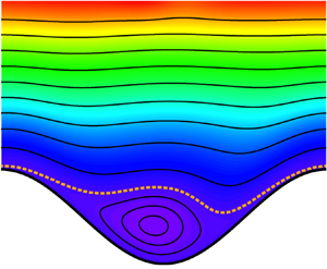
Figure 5. (a) Velocity profiles $\mathcal {U}^0$, $\hat {\mathcal {U}}$ and $\mathcal {U}^{d_e}$ introduced in the self-consistent calculation. These two last functions overlap in the upper part of their profiles, i.e. possess the same hydrodynamic roughness $z_e$ (dashed orange lines). Here, computation done for $k\zeta =0.88$ (see figure 6a) and $k\nu /u_* = 0.05$, which converges to $d_e u_*/\nu \simeq 130$. (b) Sinusoidal approximation of the surface of a periodic array of touching grains, setting $\lambda = d$. (c) Isocontours of the dimensionless streamfunction $k \varPsi /u_*$ (see Appendix B) above a modulated surface (in white), when $k\zeta =0.88$ and $k\nu /u_* = 0.05$. The flow is from left to right. Colour code: $k \varPsi /u_*$ is increasing from blue to red in the background; and the dashed orange curve corresponds to $k \varPsi /u_* = 0$.

The idea is then to use instead the looped expansion introduced in § 2.4. We start with the smooth base velocity profile $\mathcal {U}^0$, i.e. computed from (2.9) with $\eta _d=0$ in (2.7), choose a value of $k\zeta$ and iterate the described procedure until convergence. To avoid numerical instabilities, we use the numerical trick to approximate at each loop $\hat {\mathcal {U}}$ by the base profile $\mathcal {U}^{d_e}$ computed for a non-vanishing $d_e$, so that their hydrodynamic roughnesses are the same (figure 5a).

We show in figure 6(a) the effective roughness computed in this self-consistent manner for various values of $k\zeta$, as a function of $\lambda u_*/\nu$. It can be seen that the transition from smooth to rough regimes is indeed recovered: the roughness changes from $z_e u_*/\nu \simeq 1/7$ to a linear increase with $\lambda$. This asymptotic increase is steeper for larger values of $k \zeta$. When compared with the data on rough flat surfaces by setting $\lambda =d$, this prediction fits well the measurements when $k \zeta \simeq 0.88$ (see the red solid curve in figure 2a). Interestingly, this value corresponds to the sinusoidal approximation of the surface of a periodic array of touching grains $Z \simeq 0.14 d \cos (2 {\rm \pi}x/d )$, which gives $k \zeta \simeq 0.14 \times 2{\rm \pi} \simeq 0.88$ (red line in figure 5b).

Figure 6. (a) Dimensionless effective hydrodynamic roughness $z_e u_*/\nu$ as a function of $\lambda u_*/\nu$, computed in a self-consistent way for different values of $k\zeta$ (see legend). (b) Resulting equivalent grain size $d_e u_*/\nu$ as a function of $k \nu /u_*$ for different $k\zeta$ (same colour code as in panel a).

Although the direct and self-consistent derivations of the effective hydrodynamic roughness (dash-dotted and solid red curves in figure 2a, respectively) are both expansions at the second order in aspect ratio $k\zeta$, their range of validity is rather different. The better performance of the self-consistent approach is due to the fact that it takes into account the topography-induced velocity reduction at the scale of $\lambda$. Consistently, we can interpret the observation that the self-consistent derivation predicts a lower $z_e$ than the direct calculation, as accounting for flow recirculations at the scale of the topography reduces the effective corrugation of the bottom (figure 5c).

3.4. Superimposed sedimentary bedforms

The other situation where inner and outer roughnesses must match is that of superimposed bedforms: the outer roughness of a given level in the scale hierarchy is the inner roughness of the next one, as we illustrated with grains, ripples and dunes (figure 1a). For this purpose, the looped calculation described in § 2.4 must be initiated at some finite value of $\mathcal {R}_d$. The resulting curves are displayed in figure 7 for $k \zeta = 0.25$, a typical value for dunes at equilibrium (aspect ratio of the order of $1/12$). Figure 7 shows consistent increasing trends for larger and rougher bed. The curves start to diverge from the smooth case when $\mathcal {R}_d$ is larger than a few units. In addition, the resulting effective roughness can be further transformed into the Darcy friction factor (or skin friction) and the hydraulic resistance (or form drag) of bedforms (Engelund Reference Engelund1977; Zanke, Roland & Wurpts Reference Zanke, Roland and Wurpts2022). An empirical formula for the hydrodynamic roughness of sedimentary bedforms has been proposed by Van Rijn (Reference Van Rijn1984), which reflects the growth of the hydrodynamic roughness from a value selected by the grain diameter $d$ to a value selected by the bedform wavelength, as the aspect ratio $k\zeta$ increases. At small aspect ratio, for $k\zeta \lesssim 0.25$, which includes the typical aspect ratio of sedimentary ripples and dunes, the looped calculation performed here turns out to be recovering values close to this empirical prediction.

Figure 7. Self-consistent calculation of the effective roughness vs bedform wavelength (a) and the equivalent grain size vs bedform wavelength (b). These are computed for a perturbation of various surface roughness $\mathcal {R}_d$ encoded by different colours (see legend for the colour code in both panels) and with an aspect ratio $k\zeta \simeq 0.25$, typically representative of sedimentary dunes. Dashed lines correspond to the moment at which $\lambda$ becomes smaller than $d$.

This situation of multi-scaled pattern is particularly relevant in the sub-aquatic case, as well as for low-pressure – e.g. planetary – gaseous environments, which provide viscous or transitional conditions (Colombini & Stocchino Reference Colombini and Stocchino2011; Jia, Andreotti & Claudin Reference Jia, Andreotti and Claudin2017; Durán Vinent et al. Reference Durán Vinent, Andreotti, Claudin and Winter2019; Andreotti et al. Reference Andreotti, Claudin, Iversen, Merrison and Rasmussen2021; Gunn & Jerolmack Reference Gunn and Jerolmack2022). We shall illustrate here how to apply the present results to the emblematic example of Martian dunes and ripples (figure 1b,c). The dunes, whose typical length is of the order of a few hundreds of metres, exhibit large metre-scale ripples on their surface; these ripples themselves are superimposed with decimetre-scale small ripples (Lapôtre et al. Reference Lapôtre2016Reference Lapôtre, Ewing, Weitz, Lewis, Lamb, Ehlmann and Rubin2018). A hydrodynamic-based explanation for the existence of these intermediate bedforms has been proposed by Durán Vinent et al. (Reference Durán Vinent, Andreotti, Claudin and Winter2019), and verified by Rubanenko et al. (Reference Rubanenko, Lapôtre, Ewing, Fenton and Gunn2022): the anomaly associated with the laminar–turbulent transition creates a forbidden gap in wavelength that stops the coarsening of the most unstable mode. As discussed above, this anomaly is present in the smooth regime only. Estimating Martian conditions with a grain size $d \simeq 100$ $\mathrm {\mu }$m, a shear velocity $u_* \simeq 0.5$ m s$^{-1}$ and a viscosity $\nu \simeq 10^{-3}$ m$^2$ s$^{-1}$, one obtains $\mathcal {R}_d \simeq 0.05$, i.e. a hydrodynamically smooth granular bed. The question is then to evaluate, for the large metre-scale ripples, the hydrodynamic roughness induced by their superimposed small ripples. Taking, for these small ripples, a wavelength $\lambda \simeq 0.1$ m and an aspect ratio of the order of $1/20$, i.e. $k\zeta \simeq 0.15$, one obtains, with $\lambda u_*/\nu \simeq 50$, an effective roughness $z_e u_*/\nu \simeq 0.2$ corresponding to an equivalent sand grain Reynolds number $\mathcal {R}_{d_e} \simeq 5$. This indicates that the flow over the large ripples is indeed in the smooth regime, consistently with the hypothesis of Durán Vinent et al. (Reference Durán Vinent, Andreotti, Claudin and Winter2019). Now, taking for these large ripples $\lambda \simeq 3$ m, i.e. $\lambda u_*/\nu \simeq 1.5 \times 10^3$, and $k\zeta \simeq 0.25$, we see in figure 7 ($\mathcal {R}_{d} = 5$ is between the blue and black lines) an effective roughness $z_e u_*/\nu \simeq 1.5$, corresponding to an equivalent sand grain Reynolds number $\mathcal {R}_{d_e} \simeq 55$. This means that the flow over the large dunes should be considered intermediate between smooth and rough regimes. Importantly, aeolian saltation – and sediment transport in general (Van Rijn Reference Van Rijn1984) – is known to increase the sediment bed roughness, with $z_0$ of the order of a few $d$ in the terrestrial case, associated with Bagnold's focal point (Durán et al. Reference Durán, Claudin and Andreotti2011; Valance et al. Reference Valance, Rasmussen, El Moctar and Dupont2015). In low-pressure (Martian) conditions, no such measurement is available so far, but we have checked that the above conclusions are unchanged when doing this hierarchical looped calculation with an initial similar saltation-induced surface roughness.

3.5. Nonlinear size selection of dissolution bedforms

Finally, the self-consistent prediction of the effective roughness induced by a wavy surface can be used to revisit the argument given by Claudin et al. (Reference Claudin, Durán and Andreotti2017) for the selection of the aspect ratio of dissolution patterns. The instability at the origin of these bedforms is associated with the hydrodynamic anomaly on smooth modulated beds for a narrow range of wavenumbers around $k\nu /u_* \simeq 10^{-3}$. This anomaly, and thus the instability mechanism, disappears when the bed is rough enough. Because the development of the bedforms generates an effective roughness, the idea is that they would stop growing when this threshold in $\mathcal {R}_d$ is reached. Here, we can make this argument more quantitative with the proposed nonlinear calculations. The looped computation of $z_e$ equivalently provides a corresponding equivalent grain size $d_e$, which depends on $k\zeta$ (figure 6b). Experimental studies on the development of ice ripples and scallops report equilibrium shapes with the inverse Reynolds numbers in the range $k\nu /u_* \simeq 8 \times 10^{-4}\hbox{--}2 \times 10^{-3}$, and aspect ratios 6–8%, i.e. $k\zeta \simeq 0.19\hbox{--}0.25$ (Ashton & Kennedy Reference Ashton and Kennedy1972; Bushuk et al. Reference Bushuk, Yang, Winton, Msadek, Harrison, Rosati and Gudgel2019). The corresponding induced roughness reads from figure 6(b) around $d_e u_*/\nu \simeq 50$. This value is nicely consistent with the instability threshold computed for parameters relevant to the case of ice melting (Claudin et al. Reference Claudin, Durán and Andreotti2017).

4. Concluding remarks

Pursuing our goal to describe the hydrodynamic response to a bed perturbation, we have here gone one step beyond the linear order, and computed the homogeneous correction to the base flow induced by the topography. This is a quadratic effect in the amplitude of the bed elevation, thus requiring weakly nonlinear calculations. Three main results can be emphasised: we quantify how the bed corrugation increases the effective hydrodynamic roughness; we show that this effect is sensitive to the laminar–turbulent transition; this model is able to reproduce the smooth–rough transition in a self-consistent manner and can be applied to multiscale elevation profiles where inner and outer roughnesses are hierarchically nested.

The expression (3.1) shows that the effective roughness $z_e$ cannot be simply related to a single geometrical length (Schlichting & Gersten Reference Schlichting and Gersten2000; Van Rijn Reference Van Rijn1982; Raupach, Antonia & Rajagopalan Reference Raupach, Antonia and Rajagopalan1991a; Wiberg & Nelson Reference Wiberg and Nelson1992), here the amplitude $\zeta$ of the surface elevation profile. It still depends on the inner roughness of the flat surface $z_0$. Moreover, it involves a coefficient $E$ that also depends on the wavenumber of the surface profile, typically decreasing with larger $k$. Interestingly, it shows a non-monotonic behaviour for a range of wavenumber. This anomaly is larger for smoother surfaces, and disappears in the rough limit. Consistently with a similar anomaly for the stress and pressure response (Claudin et al. Reference Claudin, Durán and Andreotti2017Reference Claudin, Louge and Andreotti2021), it can be associated, in the model, with the lag between the thickness of the viscous sub-layer (parametrised by $\mathcal {R}_t$) and the pressure gradient (2.5). This anomaly plays a key role in the formation of sedimentary, dissolution or sublimation bedforms, especially in low-pressure planetary conditions (Durán Vinent et al. Reference Durán Vinent, Andreotti, Claudin and Winter2019; Bordiec et al. Reference Bordiec, Carpy, Bourgeois, Herny, Massé, Perret, Claudin, Pochat and Douté2020). However, its direct experimental evidence is limited to a series of measurements by Hanratty and co-workers (Zilker et al. Reference Zilker, Cook and Hanratty1977; Frederick & Hanratty Reference Frederick and Hanratty1988), that involve a dedicated apparatus with electro-kinetic probes to obtain the basal shear stress response. The present work suggests that the measurement of the hydrodynamic roughness induced by a sinusoidal smooth bottom, achievable by more standard and non-intrusive velocimetric techniques, could offer an alternative way to provide experimental evidence for this anomaly and allow for a better calibration of the relaxation equation (2.5). Importantly, as larger surface perturbations induce the smooth to rough transition, the self-consistent calculation of $z_e$ shows that the anomaly disappears when $k\zeta$ is too large, and the non-monotonic behaviour of the roughness is effectively observed here typically for $k\zeta \lesssim 0.05$. Finally, these results also shed light on open hydrodynamic topics associated with such transitional shear flows over a solid wall (Tuckerman, Chantry & Barkley Reference Tuckerman, Chantry and Barkley2020; Gomé, Tuckerman & Barkley Reference Gomé, Tuckerman and Barkley2022).

Numerical simulations provide another way to investigate these questions. In particular, direct numerical simulation over wavy surfaces, in the spirit of those of Maaß & Schumann (Reference Maa and Schumann1996) and De Angelis, Lombardi & Banerjee (Reference De Angelis, Lombardi and Banerjee1997), would allow one to gain a deeper understanding of Hanratty's anomaly. In such simulations, the good control of the imposed flow as well as the surface properties (wavelength, amplitude, roughness), together with a scale separation which requires a resolved viscous sub-layer much smaller than the surface wavelength, itself sufficiently smaller than the system size, is definitively challenging at relevant values of the Reynolds number, but probably reachable with current numerical techniques and computer power (Lee & Moser Reference Lee and Moser2015). The understanding and the description of the interplay between a wavy surface and the associated modulation of the viscous sublayer then remains an interesting open problem both from numerical and experimental points of view, with significant potential applications for geomorphology and geophysical flows.

Acknowledgements

We thank F. Charru, O. Durán Vinent and M. Louge for long-term collaborations on this subject of hydrodynamic response to surface topography. We acknowledge the contribution of A. Fourrière in setting a first version of these nonlinear hydrodynamic calculations. P.C. thanks W. Anderson, S. Carpy, S. Courrech du Pont, L. Couston, L. Duchemin, B. Favier and C. Narteau for discussions on Hanratty's anomaly.

Funding

P.J. was supported by National Natural Science Foundation of China (NSFC12102114) and Shenzhen Science and Technology Programme (Grant No. RCBS20200714114940144).

Declaration of interests

The authors report no conflict of interest.

Data availability

The data that support the findings of this study are available from the authors upon request.

Appendix A. Weakly nonlinear expansion

In this appendix, we provide detailed information on how to perform the weakly nonlinear expansion. The aim is to derive two sets of closed equations for the linear and homogeneous quadratic responses, which are then solved with boundary conditions at the bottom and top of the computing domain.

The weakly nonlinear expansion for $u_x$ has been given in (2.10) as follows:

(A1)\begin{equation} u_x = u_* [{\mathcal{U}}+(k\zeta) \,{\rm e}^{{\rm i}kx} U_1 + (k\zeta)^2 U_{0}], \end{equation}

with $U_1$ and $U_0$ being the modal functions, respectively, for the linear and homogeneous quadratic responses. Herein, standard notations with complex numbers are used for all quantities involved for the linear development in the sake of mathematical convenience, although only real parts are understood. However, when computing the nonlinear terms, one must go back to real notations through the transform $f \to (f+f^*)/2$, with $f^*$ being the complex conjugate of $f$. In the same way, expansions are respectively performed for the vertical velocity $u_z$, the shear stress $\tau _{xz}$, the normal stress difference $\tau _{zz} - \tau _{xx}$, the vertical component of the stress $p-\tau _{zz}$ and the dimensionless mixing length $k\ell$ as

(A2)$$\begin{gather} u_z = u_* [(k\zeta) \,{\rm e}^{{\rm i}kx} W_1], \end{gather}$$
(A3)$$\begin{gather}\tau_{xz}= \rho u_*^2 [1+(k\zeta) \,{\rm e}^{{\rm i}kx} S_{t1}+(k\zeta)^2 S_{t0}], \end{gather}$$
(A4)$$\begin{gather} \tau_{zz} - \tau_{xx} = \rho u_*^2 [(k\zeta) \,{\rm e}^{{\rm i}kx} S_{d1}+(k\zeta)^2 S_{d0}], \end{gather}$$
(A5)$$\begin{gather} p-\tau_{zz} = \rho u_*^2 \left[\tfrac{1}{3}\chi^2+(k\zeta) \,{\rm e}^{{\rm i}kx} S_{n1}+(k\zeta)^2 S_{n0}\right], \end{gather}$$
(A6)$$\begin{gather}k\ell = \varUpsilon + k\zeta \,{\rm e}^{{\rm i}kx} L_1+(k\zeta)^2 L_{0}. \end{gather}$$

Note that, as there cannot be fluid flow through the solid boundary, the term $W_0(\eta )=0$ is not included into the expansion.

With these notations, the strain rate modulus can be rewritten as

(A7)\begin{equation} |\dot \gamma|=\mathcal{U}'+(k\zeta) \,{\rm e}^{{\rm i}kx} (U_1'+{\rm i}W_1)+(k\zeta)^2 \left[U_0'+\frac{1}{\mathcal{U}'}U_1U_1^*\right], \end{equation}

and following (2.3), the stress modal functions can be expressed as

(A8)\begin{gather} S_{t1}= (2 \varUpsilon^2 \mathcal{U}'+\mathcal{R}^{{-}1}) (U_1'+{\rm i} W_1)+2 L_1 \varUpsilon \mathcal{U}'^2,\end{gather}
(A9)\begin{gather} \begin{aligned}S_{t0}&=(2 \varUpsilon^2 \mathcal{U}'+\mathcal{R}^{{-}1})U_0'+\tfrac{1}{2} L_1 \mathcal{U}'^2 L_1^*+ \varUpsilon^2 ( U_1 U_1^*+\tfrac{1}{2} (U_1'+{\rm i} W_1) (U_1'^*-{\rm i} W_1^*))\nonumber\\ &\quad +\varUpsilon ( \mathcal{U}' L_1^* (U_1'+{\rm i} W_1)+ L_1 \mathcal{U}' (U_1'^*-{\rm i} W_1^*)+2 L_0 \mathcal{U}'^2),\end{aligned}\end{gather}
(A10)\begin{gather} S_{d1}={-}\frac{4 {\rm i}}{ \mathcal{U}' } U_1, \end{gather}
(A11)\begin{gather} S_{d0}={-}2{\rm i} \varUpsilon ( \mathcal{U}' U_1 L_1^*- L_1 \mathcal{U}' U_1^*)-{\rm i} \varUpsilon^2 (U_1 (U_1'^*-{\rm i} W_1^*)-U_1^*(U_1' +{\rm i} W_1 )), \end{gather}

where $(\mathcal {R}^{-1} + \varUpsilon ^2 \mathcal {U}' ) = 1/ \mathcal {U}'$ as deduced from (2.9). Further, the modal functions for the mixing length are obtained as

(A12)\begin{align} \frac{L_1}{\kappa}&=\frac{1}{2} \,{\rm e}^{-(\eta+s\eta_d) ({\mathcal{R}}/{\mathcal{R}_t^0})} \left\{ (\eta+r\eta_d) \frac{\mathcal{R}}{\mathcal{R}_t^0} [ 2 (\eta+s\eta_d )R_{t1} +(\eta+s\eta_d ) S_{t1}-2 ] +2 \right\}-1,\end{align}
(A13)\begin{align} \frac{L_0}{\kappa}&={-}\frac{1}{16} \frac{\mathcal{R}}{\mathcal{R}_t^0} \, {\rm e}^{-(\eta+s\eta_d) ({\mathcal{R}}/{\mathcal{R}_t^0})} \left\{ 4 \left[ (\eta+r\eta_d) \left(\frac{\mathcal{R}}{\mathcal{R}_t^0} - 2 S_{t0} (\eta+s\eta_d)\right) -2 \right.\right. \nonumber\\ &\quad \left.+\,(R_{t1}^*+R_{t1} +(S_{t1} + S_{t1}^*)/2) \left((\eta+r\eta_d) + (\eta+s\eta_d)-(\eta+r\eta_d)(\eta+s\eta_d) \frac{\mathcal{R}}{\mathcal{R}_t^0}\right) \right]\nonumber\\ &\quad +4 (\eta+r\eta_d) (\eta+s\eta_d) R_{t1}^* R_{t1} S_{t1} \left((\eta+s\eta_d) \frac{\mathcal{R}}{\mathcal{R}_t^0}-2 \right) \left((\eta+s\eta_d) \frac{\mathcal{R}}{\mathcal{R}_t^0}-1\right) \nonumber\\ &\quad +\left.(\eta+r\eta_d) (\eta+s\eta_d) S_{t1}^* \left[ 2 R_{t1} \left((\eta+s\eta_d) \frac{\mathcal{R}}{\mathcal{R}_t^0}-1\right) + (\eta+s\eta_d) \frac{\mathcal{R}}{\mathcal{R}_t^0} S_{t1}+S_{t1}\right] \right\}, \end{align}

where

(A14)\begin{equation} R_{t1}=\frac{{\rm i}b}{\mathcal{R}+{\rm i}a}(S_{d1}+S_{n1}) \end{equation}

is defined from the transitional Reynolds number $\mathcal {R}_t/\mathcal {R}_t^0=1-(k\zeta ) \,{\rm e}^{{\rm i}kx} R_{t1}$ and deduced from Hanratty's relaxation relation (2.5).

Introducing the above expansions into the Navier–Stokes equations (2.1)–(2.2), we derive the differential equations at linear and homogeneous–quadratic orders on the modal functions. The linear components yield

(A15)$$\begin{gather} U_1' ={-} {\rm i} W_1 +\frac{S_{t1}-2 \varUpsilon \mathcal{U}'^2 L_1}{{\mathcal{R}}^{{-}1}+2 \varUpsilon^2 \mathcal{U}' }, \end{gather}$$
(A16)$$\begin{gather}W_1'={-}{\rm i}U_1, \end{gather}$$
(A17)$$\begin{gather} S_{t1}'={\rm i}\mathcal{U} U_1 +\mathcal{U}'W_1+{\rm i}(S_{n1}+S_{d1}), \end{gather}$$
(A18)$$\begin{gather}S_{n1}'={-}{\rm i}\mathcal{U} W_1 + {\rm i}S_{t1}, \end{gather}$$

where the expression giving $U_1'$ (A15) results from the shear stress modal function $S_{t1}$ (A8). This is the result derived in Claudin et al. (Reference Claudin, Durán and Andreotti2017). For the new homogeneous–quadratic order, the differential equations of the modal functions are

(A19)\begin{align} U_0'&=\frac{1}{(2 \varUpsilon^2 \mathcal{U}'+\mathcal{R}^{{-}1})}\left[ S_{t0}-\frac{1}{2} L_1 \mathcal{U}'^2 L_1^*- \varUpsilon^2 \left( U_1 U_1^*+\frac{1}{2} (U_1'+{\rm i} W_1) (U_1'^*-{\rm i} W_1^*)\right)\right.\nonumber\\ &\quad -\left.\varUpsilon ( \mathcal{U}' L_1^* (U_1'+{\rm i} W_1)+ L_1 \mathcal{U}' (U_1'^*-{\rm i} W_1^*)+2 L_0 \mathcal{U}'^2)\vphantom{\frac{1}{2}}\right], \end{align}
(A20)\begin{gather} S_{t0}'= \tfrac{1}{4}(W_1U_1'^*+W_1^*U_1'), \end{gather}
(A21)\begin{gather} S_{n0}'= \tfrac{1}{2} i (U_1W_1^*-U_1^*W_1), \end{gather}

where, as in the linear order, the expression for $U_0'$ (A19) is deduced from the shear stress modal function $S_{t0}$ (A9). Note that $S_{n0}$ does not enter the equations for $U'_{0}$ and $S'_{t0}$, and it thus decouples from the present problem focused on the computation of $U_0$. Furthermore, the stress functions $S_{t0}$ and $S_{n0}$ can be obtained by integration over $\eta$, once the linear order ($U_1$ and $W_1$) is known.

The integration of the two above sets of differential equations (A15)–(A21) requires boundary conditions at the substrate surface and at infinity. The upper boundary corresponds to the limit $\eta \to \infty$, in which the vertical flux of momentum vanishes asymptotically. This means that the corrections to the vertical velocity and to the shear stress must tend to zero at both orders: (i) $W_1(\infty )=0$ and (ii) $S_{t1}(\infty )=0$, $S_{t0}(\infty )=0$. In practice, we introduce a finite height $H$ (or $\eta _H \equiv kH$), at which we impose a null vertical velocity and a constant tangential stress $-\rho u_*^2$, so that $W_1(\eta _H) = 0$ and $S_{t1}(\eta _H) = 0$, $S_{t0}(\eta _H) = 0$. Then, we consider the limit $H \to +\infty$, i.e. when the results become independent of $H$. Both components of the velocity should vanish at the substrate surface, i.e. for $\eta =kZ$. The condition $u_x(x,kZ)=0$ then yields

(A22)$$\begin{gather} U_1(0) ={-}\mathcal{U}'(0), \end{gather}$$
(A23)$$\begin{gather}U_0(0) ={-}\tfrac{1}{4}\mathcal{U}''(0) - \tfrac{1}{4}U_1'(0) - \tfrac{1}{4}U_1'^*(0). \end{gather}$$

Similarly, for $u_z(x,kZ)=0$, we get $W_1(0) = 0$.

The differential equations (A15)–(A18) for the functions associated with the linear terms are first solved by integrating with the corresponding boundary conditions. The solutions are then used to solve equations (A19)–(A20) for the functions associated with the homogeneous terms.

Appendix B. Shifted representations and streamfunction

A ‘shifted’ representation of the modal functions is used in some parts of the paper, noted with an additional tilde. In this study, all fields are expanded up to the homogeneous second order in $k\zeta$ in a non-shifted representation as in (2.10) for the streamwise velocity. For some of the graphs, we sometimes prefer to present the velocity profiles in the shifted representation as

(B1)\begin{equation} u_x= {u_*} [\mathcal{U} (\xi)+(k\zeta) \,{\rm e}^{{\rm i}kx} \tilde U_1(\xi )+(k\zeta)^2 \tilde U_0(\xi )], \end{equation}

where $\xi = \eta -k\zeta \,{\rm e}^{{\rm i}kx}$. Expanding the functions $\tilde {f} (\eta -k\zeta \,{\rm e}^{{\rm i}kx})$ with respect to $k\zeta$, one obtains

(B2)\begin{equation} \tilde U_0=U_0+\tfrac{1}{4}\mathcal{U}''+ \tfrac{1}{4}(U_1' + U_1'^* ), \end{equation}

where $\tilde U_1 =U_1+\mathcal {U}'$ has been given in Fourrière et al. (Reference Fourrière, Claudin and Andreotti2010). The shifted representations for the other fields work in a similar fashion, except that there could be no base profile as $\mathcal {U}$ in the expressions.

To compute the streamlines, we introduce the streamfunction $\varPsi (x,z)$. In the shifted representation, one solution is $\varPsi =\int _0^{z} u_x \,{\rm d} \hat {z}$, and this integral is computed between the surface $\hat {z} = 0$ and some vertical distance $\hat {z} = z$. Following (B1), one then has

(B3)\begin{equation} \varPsi=\frac{u_*}{k}\int_0^{\xi} [\mathcal{U} (\hat{\xi})+(k\zeta) \,{\rm e}^{{\rm i}kx} \tilde U_1(\hat{\xi} )+(k\zeta)^2 \tilde U_0(\hat{\xi} )]\,{\rm d} \hat{\xi}. \end{equation}

Introducing $\tilde U_1 =U_1+\mathcal {U}'$ and (B2), it gives

(B4)\begin{equation} \varPsi=\frac{u_*}{k}\int_0^{\eta} \left[\mathcal{U} +(k\zeta)^2 \left( U_0+\frac{1}{4}\mathcal{U}''+ \frac{1}{4}(U_1' + U_1'^* )\right) +(k\zeta)\, {\rm e}^{{\rm i}kx} ( {\rm i} W'_1+ \mathcal{U}' )\right]{\rm d} \hat{\eta}, \end{equation}

where we have used the relation at the linear order $W_1'=-{\rm i}U_1$ (A17). Consequently, one obtains a dimensionless streamfunction $k\varPsi /u_*$

(B5)\begin{align} \frac{k \varPsi}{u_*}&=\int_{0}^{\eta} (\mathcal{U} + (k\zeta)^2 U_0 )\,{\rm d} \hat{\eta} + \frac{1}{4} (k\zeta)^2 [\mathcal{U}'+ (U_1 + U_1^* )+ \mathcal{U}'(0) ]\nonumber\\ &\quad +(k\zeta) \,{\rm e}^{{\rm i}kx}( {\rm i} W_1+ \mathcal{U} ), \end{align}

where we have used the boundary conditions $\mathcal {U}(0) =0$, $W_1(0)=0$ and $U_1(0) = -\mathcal {U}'(0)$.

For the streamfunction in the self-consistent expansion analysis (§ 2.4), it should be noted that in this equation the homogeneous velocity of the base state $\mathcal {U}$ in the integration should be estimated with $\mathcal {R}_d = 0$ as $\mathcal {U}^0$, and that the other quantities should be estimated with $\mathcal {R}_d = d_e u_*/\nu$. Here, for the plots (figure 5c), only the real part of (B5) is considered.

Appendix C. Asymptotic regimes of the roughness coefficient $E$

In this appendix, we provide more details in the scaling arguments for the viscous and turbulent regimes of the roughness coefficient $E$.

C.1. Viscous regime

In the viscous response limit, the flow is governed by the Stokes equations. At the linear order in $k\zeta$, the corresponding equations on the modal functions are

(C1)$$\begin{gather} U_1' ={-} {\rm i} W_1 +\frac{S_{t1}}{{\mathcal{R}}^{{-}1} }, \end{gather}$$
(C2)$$\begin{gather}W_1'={-}{\rm i}U_1, \end{gather}$$
(C3)$$\begin{gather}S_{t1}'= {\rm i}(S_{n1}+S_{d1}), \end{gather}$$
(C4)$$\begin{gather}S_{n1}'= {\rm i}S_{t1}. \end{gather}$$

At the homogeneous quadratic order, we have

(C5)$$\begin{gather} U_0'=\frac{S_{t0}}{\mathcal{R}^{{-}1}}, \end{gather}$$
(C6)$$\begin{gather}S_{t0}'= 0, \end{gather}$$
(C7)$$\begin{gather}S_{n0}'=0. \end{gather}$$

Using the boundary condition $S_{t0}(\eta _H)=0$, we can deduce from (C6) that $S_{t0} = 0$. From (C5), we therefore obtain $U'_0 = 0$, i.e. $U_0$ is a constant. Considering the no-slip boundary condition at the surface (A23), we have

(C8)\begin{equation} U_0=U_0(0) ={-}\tfrac{1}{4}\mathcal{U}''(0) - \tfrac{1}{4}U_1'(0) - \tfrac{1}{4}U_1'^*(0). \end{equation}

In this viscous limit $\mathcal {U}' = \mathcal {R}$, independent of $\eta$, and therefore $\mathcal {U}''(0) = 0$. From (C1), we deduce

(C9)\begin{equation} U_1'(0) = {S_{t1}(0)}{{\mathcal{R}}}, \end{equation}

where we have used the condition $W_1 (0) = 0$. Considering $S_{t1}(0) =\mathcal {A} + {\rm i} \mathcal {B}$, we then have

(C10)\begin{equation} U_0={-} \tfrac{1}{4}(S_{t1}(0) + S_{t1}^*(0)) ={-} \tfrac{1}{2} \mathcal{R} \,\mathcal{A}, \end{equation}

and thus

(C11)\begin{equation} E ={-} U_0 = \tfrac{1}{2} \mathcal{R} \, \mathcal{A} . \end{equation}

C.2. Turbulent regime

In this limit, one can infer an expression for $E(kz_0)$ estimating $U_0$ at a typical (dimensionless) height $\eta \sim 1$, above which its profile becomes constant (figure 3a). For that purpose, we combine estimations of the shear stress from the momentum balance (2.2) and from the turbulent closure (2.3).

Let us start with (2.3), we can express in this limit as $\tau \sim \rho \ell ^2 ( \boldsymbol {\nabla } u )^2$. For the homogeneous correction in $(k\zeta )^2$, it writes

(C12)\begin{equation} S_{t0} = \varUpsilon^2 \mathcal{U}' U_0' + L_0^2 \mathcal{U}'^2 + \varUpsilon^2 U_1^2 + \varUpsilon^2 U_1'^2 + \varUpsilon L_1 \mathcal{U}' U_1' + L_1^2 \mathcal{U}'^2, \end{equation}

where the first term on the right-hand side comes from the velocity gradient taken at the quadratic order $U_0$, with all other factors taken in the base state ($\varUpsilon$ for the dimensionless mixing length and $\mathcal {U}$ for the dimensionless velocity). The second term is the modulated mixing length at this order 0, and the base velocity. The other contributions come from combinations of terms at linear order. A first possibility is to take a base mixing length with velocity horizontal and vertical derivatives. A second possibility is with a modulated mixing length and (vertical) velocity derivative. A last possibility is to take a modulated mixing length with a base velocity. One can recognise all these terms in (A9), properly expressed with complex notations and correct prefactors. We can estimate their scaling behaviour having in mind that, in this rough turbulent limit, we have: $\varUpsilon \sim \kappa \eta$, $\mathcal {U}' \sim 1/\varUpsilon$, $L_1 \sim \kappa$ and $L_0 \to 0$. Also, we estimate quantities and vertical derivatives at the scale $\eta \sim 1$, so that $\mathcal {U}' \sim \mathcal {U}/\eta \sim \mathcal {U}$ (and similarly for $U_1$ and $U_0$). This essentially leads to $S_{t0} \sim U_0 + U_1^2 + U_1 + \mbox {Cst}$.

References

Andreotti, B. 2004 A two-species model of aeolian sand transport. J. Fluid Mech. 510, 4770.CrossRefGoogle Scholar
Andreotti, B., Claudin, P., Iversen, J.J., Merrison, J.P. & Rasmussen, K.R. 2021 A lower-than-expected saltation threshold at martian pressure and below. Proc. Natl Acad. Sci. USA 118 (5), e2012386118.CrossRefGoogle ScholarPubMed
Ashton, G.D. & Kennedy, J.F. 1972 Ripples on underside of river ice covers. J. Hydraul. Div. 98 (9), 16031624.CrossRefGoogle Scholar
Aulnette, M., Rabaud, M. & Moisy, F. 2019 Wind-sustained viscous solitons. Phys. Rev. Fluids 4 (8), 084003.CrossRefGoogle Scholar
Ayotte, K.W., Xu, D.P. & Taylor, P.A. 1994 The impact of turbulence closure schemes on predictions of the mixed spectral finite-difference model for flow over topography. Boundary-Layer Meteorol 68 (1), 133.CrossRefGoogle Scholar
Bagnold, R.A. 1941 The Physics of Blown Sand and Desert Dunes. Methuen.Google Scholar
Benjamin, T.B. 1959 Shearing flow over a wavy boundary. J. Fluid Mech. 6 (2), 161205.CrossRefGoogle Scholar
Bordiec, M., Carpy, S., Bourgeois, O., Herny, C., Massé, M., Perret, L., Claudin, P., Pochat, S. & Douté, S. 2020 Sublimation waves: geomorphic markers of interactions between icy planetary surfaces and winds. Earth-Sci. Rev. 211, 103350.CrossRefGoogle Scholar
Bradley, E.F. 1980 An experimental study of the profiles of wind speed, shearing stress and turbulence at the crest of a large hill. Q. J. R. Meteorol. Soc. 106 (447), 101123.CrossRefGoogle Scholar
Brown, S., Nickling, W.G. & Gillies, J.A. 2008 A wind tunnel examination of shear stress partitioning for an assortment of surface roughness distributions. J. Geophys. Res. Earth Surf. 113, F02S06.CrossRefGoogle Scholar
Bushuk, M., Yang, X., Winton, M., Msadek, R., Harrison, M., Rosati, A. & Gudgel, R. 2019 The value of sustained ocean observations for sea ice predictions in the Barents Sea. J. Clim. 32 (20), 70177035.CrossRefGoogle Scholar
Charru, F., Andreotti, B. & Claudin, P. 2013 Sand ripples and dunes. Annu. Rev. Fluid Mech. 45, 469493.CrossRefGoogle Scholar
Charru, F. & Hinch, E.J. 2000 ‘Phase diagram’ of interfacial instabilities in a two-layer Couette flow and mechanism of the long-wave instability. J. Fluid Mech. 414, 195223.CrossRefGoogle Scholar
Cheng, H., Hayden, P., Robins, A.G. & Castro, I.P. 2007 Flow over cube arrays of different packing densities. J. Wind Engng Ind. Aerodyn. 95 (8), 715740.CrossRefGoogle Scholar
Choi, H., Jeon, W.P. & Kim, J. 2008 Control of flow over a bluff body. Annu. Rev. Fluid Mech. 40, 113139.CrossRefGoogle Scholar
Chung, D., Hutchins, N., Schultz, M.P. & Flack, K.A. 2021 Predicting the drag of rough surfaces. Annu. Rev. Fluid Mech. 53, 439471.CrossRefGoogle Scholar
Claudin, P., Durán, O. & Andreotti, B. 2017 Dissolution instability and roughening transition. J. Fluid Mech. 832, R2.CrossRefGoogle Scholar
Claudin, P., Louge, M. & Andreotti, B. 2021 Basal pressure variations induced by a turbulent flow over a wavy surface. Front. Phys. 9, 682564.CrossRefGoogle Scholar
Colombini, M. 2004 Revisiting the linear theory of sand dune formation. J. Fluid Mech. 502, 116.CrossRefGoogle Scholar
Colombini, M. & Stocchino, A. 2011 Ripple and dune formation in rivers. J. Fluid Mech. 673, 121131.CrossRefGoogle Scholar
Crago, R.D., Okello, W. & Jasinski, M.F. 2012 Equations for the drag force and aerodynamic roughness length of urban areas with random building heights. Boundary-Layer Meteorol. 145 (3), 423437.CrossRefGoogle Scholar
De Angelis, V., Lombardi, P. & Banerjee, S. 1997 Direct numerical simulation of turbulent flow over a wavy wall. Phys. Fluids 9 (8), 24292442.CrossRefGoogle Scholar
De Langre, E. 2008 Effects of wind on plants. Annu. Rev. Fluid Mech. 40, 141168.CrossRefGoogle Scholar
Dong, Z., Liu, X. & Wang, X. 2002 Aerodynamic roughness of gravel surfaces. Geomorphology 43 (1–2), 1731.CrossRefGoogle Scholar
Durán, O., Claudin, P. & Andreotti, B. 2011 On aeolian transport: grain-scale interactions, dynamical mechanisms and scaling laws. Aeolian Res. 3 (3), 243270.CrossRefGoogle Scholar
Durán Vinent, O., Andreotti, B., Claudin, P. & Winter, C. 2019 A unified model of ripples and dunes in water and planetary environments. Nat. Geosci. 12 (5), 345350.CrossRefGoogle Scholar
Elbelrhiti, H., Claudin, P. & Andreotti, B. 2005 Field evidence for surface-wave-induced instability of sand dunes. Nature 437 (7059), 720723.CrossRefGoogle ScholarPubMed
Engelund, F. 1977 Hydraulic resistance for flow over dunes. Prog. Rep. 44, 19M20.Google Scholar
Fang, C. & Sill, B.L. 1992 Aerodynamic roughness length: correlation with roughness elements. J. Wind Engng Ind. Aerodyn. 41 (1–3), 449460.CrossRefGoogle Scholar
Finnigan, J.J. 1988 Air flow over complex terrain. Flow and Transport in the Natural Environment: Advances and Applications, pp. 183–229. Springer.CrossRefGoogle Scholar
Flack, K.A & Schultz, M.P 2010 Review of hydraulic roughness scales in the fully rough regime. J. Fluids Engng 132 (4), 041203.CrossRefGoogle Scholar
Fourrière, A., Claudin, P. & Andreotti, B. 2010 Bedforms in a turbulent stream: formation of ripples by primary linear instability and of dunes by nonlinear pattern coarsening. J. Fluid Mech. 649, 287328.CrossRefGoogle Scholar
Frederick, K.A. & Hanratty, T.J. 1988 Velocity measurements for a turbulent nonseparated flow over solid waves. Exp. Fluids 6 (7), 477486.CrossRefGoogle Scholar
Gillette, D.A., Marticorena, B. & Bergametti, G. 1998 Change in the aerodynamic roughness height by saltating grains: experimental assessment, test of theory, and operational parameterization. J. Geophys. Res. Atmos. 103 (D6), 62036209.CrossRefGoogle Scholar
Gillies, J.A., Nickling, W.G. & King, J. 2007 Shear stress partitioning in large patches of roughness in the atmospheric inertial sublayer. Boundary-Layer Meteorol. 122 (2), 367396.CrossRefGoogle Scholar
Gomé, S., Tuckerman, L.S. & Barkley, D. 2022 Extreme events in transitional turbulence. Phil. Trans. R. Soc. A 380 (2226), 20210036.CrossRefGoogle ScholarPubMed
Gunn, A. & Jerolmack, D.J. 2022 Conditions for aeolian transport in the solar system. Nat. Astron. 6 (8), 923929.CrossRefGoogle Scholar
Han, C., Ma, Y., Su, Z., Chen, X., Zhang, L., Li, M. & Sun, F. 2015 Estimates of effective aerodynamic roughness length over mountainous areas of the tibetan plateau. Q. J. R. Meteorol. Soc. 141 (689), 14571465.CrossRefGoogle Scholar
Hanratty, T.J. 1981 Stability of surfaces that are dissolving or being formed by convective diffusion. Annu. Rev. Fluid Mech. 13 (1), 231252.CrossRefGoogle Scholar
Hobson, J.M., Wood, N. & Brown, A.R. 1999 Large-eddy simulations of neutrally stratified flow over surfaces with spatially varying roughness length. Q. J. R. Meteorol. Soc. 125 (558), 19371958.CrossRefGoogle Scholar
Hunt, J.C.R., Leibovich, S. & Richards, K.J. 1988 Turbulent shear flows over low hills. Q. J. R. Meteorol. Soc. 114 (484), 14351470.CrossRefGoogle Scholar
Jackson, P.S. & Hunt, J.C.R. 1975 Turbulent wind flow over a low hill. Q. J. R. Meteorol. Soc. 101 (430), 929955.CrossRefGoogle Scholar
Jacobs, S.J. 1989 Effective roughness length for turbulent flow over a wavy surface. J. Phys. Oceanogr. 19 (7), 9981010.2.0.CO;2>CrossRefGoogle Scholar
Jasinski, M.F. & Crago, R.D. 1999 Estimation of vegetation aerodynamic roughness of natural regions using frontal area density determined from satellite imagery. Agric. Forest Meteorol. 94 (1), 6577.CrossRefGoogle Scholar
Jia, P., Andreotti, B. & Claudin, P. 2017 Giant ripples on comet 67P/Churyumov–Gerasimenko sculpted by sunset thermal wind. Proc. Natl Acad. Sci. USA 114 (10), 25092514.CrossRefGoogle ScholarPubMed
Jiménez, J. 2004 Turbulent flows over rough walls. Annu. Rev. Fluid Mech. 36, 173196.CrossRefGoogle Scholar
Johnson, P.L. & Johnston, J.P. 1989 Active and inactive motions in a turbulent boundary layer-interactions with free-stream turbulence. In 7th Symposium on Turbulent Shear Flows (Stanford, CA), vol. 2, pp. 20–22. Pennsylvania State University.Google Scholar
Kadivar, M., Tormey, D. & McGranaghan, G. 2021 A review on turbulent flow over rough surfaces: fundamentals and theories. Intl J. Thermofluids 10, 100077.CrossRefGoogle Scholar
Kametani, Y., Fukagata, K., Örlü, R. & Schlatter, P. 2015 Effect of uniform blowing/suction in a turbulent boundary layer at moderate Reynolds number. Intl J. Heat Fluid Flow 55, 132142.CrossRefGoogle Scholar
Kamphuis, J.W. 1974 Determination of sand roughness for fixed beds. J. Hydraul. Res. 12 (2), 193203.CrossRefGoogle Scholar
Kent, C.W., Grimmond, S. & Gatey, D. 2017 Aerodynamic roughness parameters in cities: inclusion of vegetation. J. Wind Engng Ind. Aerodyn. 169, 168176.CrossRefGoogle Scholar
King, J., Nickling, W.G. & Gillies, J.A. 2006 Aeolian shear stress ratio measurements within mesquite-dominated landscapes of the Chihuahuan Desert, New Mexico, USA. Geomorphology 82 (3–4), 229244.CrossRefGoogle Scholar
Lancaster, N. & Baas, A. 1998 Influence of vegetation cover on sand transport by wind: field studies at Owens Lake, California. Earth Surf. Process. Landf. 23 (1), 6982.3.0.CO;2-G>CrossRefGoogle Scholar
Lapôtre, M., et al. 2016 Large wind ripples on Mars: a record of atmospheric evolution. Science 353 (6294), 5558.CrossRefGoogle Scholar
Lapôtre, M.G.A., Ewing, R.C., Weitz, C.M., Lewis, K.W., Lamb, M.P., Ehlmann, B.L. & Rubin, D.M. 2018 Morphologic diversity of martian ripples: implications for large-ripple formation. Geophys. Res. Lett. 45 (19), 10229.CrossRefGoogle Scholar
Lee, M. & Moser, R.D. 2015 Direct numerical simulation of turbulent channel flow up to $Re_{\tau } \approx 5200$. J. Fluid Mech. 774, 395415.CrossRefGoogle Scholar
Maa, C. & Schumann, U. 1996 Direct numerical simulation of separated turbulent flow over a wavy boundary. Flow Simulation with High-Performance Computers II: DFG Priority Research Programme Results 1993–1995, pp. 227–241. Vieweg+Teubner.CrossRefGoogle Scholar
Maat, N., Kraan, C. & Oost, W.A. 1991 The roughness of wind waves. Boundary-Layer Meteorol. 54 (1), 89103.CrossRefGoogle Scholar
Marticorena, B. & Bergametti, G. 1995 Modeling the atmospheric dust cycle: 1. Design of a soil-derived dust emission scheme. J. Geophys. Res. Atmos. 100 (D8), 1641516430.CrossRefGoogle Scholar
Narteau, C., Zhang, D., Rozier, O. & Claudin, P. 2009 Setting the length and time scales of a cellular automaton dune model from the analysis of superimposed bed forms. J. Geophys. Res. Earth Surf. 114 (F3), F03006.CrossRefGoogle Scholar
Nield, J.M., et al. 2013 Estimating aerodynamic roughness over complex surface terrain. J. Geophys. Res. Atmos. 118 (23), 12948.CrossRefGoogle Scholar
Nikuradse, J. 1933 Laws of flow in rough pipes. NACA Tech. Mem. 1292.Google Scholar
Owen, P.R. 1964 Saltation of uniform grains in air. J. Fluid Mech. 20 (2), 225242.CrossRefGoogle Scholar
Park, J. & Choi, H. 1999 Effects of uniform blowing or suction from a spanwise slot on a turbulent boundary layer flow. Phys. Fluids 11 (10), 30953105.CrossRefGoogle Scholar
Paul-Limoges, E., Christen, A., Coops, N.C., Black, T.A. & Trofymow, J.A. 2013 Estimation of aerodynamic roughness of a harvested Douglas-fir forest using airborne LiDAR. Remote Sens. Environ. 136, 225233.CrossRefGoogle Scholar
Perrard, S., Lozano-Durán, A., Rabaud, M., Benzaquen, M. & Moisy, F. 2019 Turbulent windprint on a liquid surface. J. Fluid Mech. 873, 10201054.CrossRefGoogle Scholar
Pope, S.B. 2000 Turbulent Flows. Cambridge University Press.CrossRefGoogle Scholar
Prandtl, L. 1925 Bericht über untersuchungen zur ausgebildeten turbulenz. Z. Angew. Math. Mech. 5 (2), 136139.CrossRefGoogle Scholar
Prigent, C., Tegen, I., Aires, F., Marticorena, B. & Zribi, M. 2005 Estimation of the aerodynamic roughness length in arid and semi-arid regions over the globe with the ERS scatterometer. J. Geophys. Res. Atmos. 110 (D9), D09205.CrossRefGoogle Scholar
Raupach, M.R. 1991 Saltation layers, vegetation canopies and roughness lengths. In Aeolian Grain Transport 1, pp. 83–96. Springer.CrossRefGoogle Scholar
Raupach, M.R. 1992 Drag and drag partition on rough surfaces. Boundary-Layer Meteorol. 60 (4), 375395.CrossRefGoogle Scholar
Raupach, M.R., Antonia, R.A. & Rajagopalan, S. 1991 a Rough-wall turbulent boundary layers. Appl. Mech. Rev. 44 (1), 125.CrossRefGoogle Scholar
Raupach, M.R., Antonia, R.A. & Rajagopalan, S. 1991 b Rough-wall turbulent boundary layers. Appl. Mech. Rev. 44 (1), 125.CrossRefGoogle Scholar
Raupach, M.R., Gillette, D.A. & Leys, J.F. 1993 The effect of roughness elements on wind erosion threshold. J. Geophys. Res. Atmos. 98 (D2), 30233029.CrossRefGoogle Scholar
Richards, K.J. 1980 The formation of ripples and dunes on an erodible bed. J. Fluid Mech. 99 (3), 597618.CrossRefGoogle Scholar
Rubanenko, L., Lapôtre, M.G.A., Ewing, R.C., Fenton, L.K. & Gunn, A. 2022 A distinct ripple-formation regime on Mars revealed by the morphometrics of barchan dunes. Nat. Commun. 13 (1), 7156.CrossRefGoogle ScholarPubMed
Sadique, J., Yang, X.I.A., Meneveau, C. & Mittal, R. 2017 Aerodynamic properties of rough surfaces with high aspect-ratio roughness elements: effect of aspect ratio and arrangements. Boundary-Layer Meteorol. 163 (2), 203224.CrossRefGoogle Scholar
Schlichting, H. 1937 Experimental investigation of the problem of surface roughness. NACA Tech. Mem. 823.Google Scholar
Schlichting, H. & Gersten, K. 2000 Boundary Layer Theory, 8th edn. Springer.CrossRefGoogle Scholar
Schmid, H.P. & Bünzli, B. 1995 The influence of surface texture on the effective roughness length. Q. J. R. Meteorol. Soc. 121 (521), 121.CrossRefGoogle Scholar
Schultz, M.P. & Flack, K.A. 2009 Turbulent boundary layers on a systematically varied rough wall. Phys. Fluids 21 (1), 015104.CrossRefGoogle Scholar
Sherman, D.J. & Farrell, E.J. 2008 Aerodynamic roughness lengths over movable beds: comparison of wind tunnel and field data. J. Geophys. Res. Earth Surf. 113 (F2), F02S08.CrossRefGoogle Scholar
Smeets, C.J.P.P. & Van den Broeke, M.R. 2008 Temporal and spatial variations of the aerodynamic roughness length in the ablation zone of the greenland ice sheet. Boundary-Layer Meteorol. 128 (3), 315338.CrossRefGoogle Scholar
Sykes, R.I. 1980 An asymptotic theory of incompressible turbulent boundary layer flow over a small hump. J. Fluid Mech. 101 (3), 647670.CrossRefGoogle Scholar
Taylor, P.A., Gent, P.R. & Keen, J.M. 1976 Some numerical solutions for turbulent boundary-layer flow above fixed, rough, wavy surfaces. Geophys. J. Intl 44 (1), 177201.CrossRefGoogle Scholar
Taylor, P.A., Sykes, R.I. & Mason, P.J. 1989 On the parameterization of drag over small-scale topography in neutrally-stratified boundary-layer flow. Boundary-Layer Meteorol. 48 (4), 409422.CrossRefGoogle Scholar
Tsai, J.L., Tsuang, B.J., Lu, P.S., Chang, K.H., Yao, M.H. & Shen, Y. 2010 Measurements of aerodynamic roughness, bowen ratio, and atmospheric surface layer height by eddy covariance and tethersonde systems simultaneously over a heterogeneous rice paddy. J. Hydrometeorol. 11 (2), 452466.CrossRefGoogle Scholar
Tsuang, B.J., Tsai, J.L., Lin, M.D. & Chen, C.L. 2003 Determining aerodynamic roughness using tethersonde and heat flux measurements in an urban area over a complex terrain. Atmos. Environ. 37 (14), 19932003.CrossRefGoogle Scholar
Tuckerman, L.S., Chantry, M. & Barkley, D. 2020 Patterns in wall-bounded shear flows. Annu. Rev. Fluid Mech. 52, 343367.CrossRefGoogle Scholar
Valance, A., Rasmussen, K.R., El Moctar, A.O. & Dupont, P. 2015 The physics of aeolian sand transport. C. R. Phys. 16 (1), 105117.CrossRefGoogle Scholar
Van Driest, E.R. 1956 On turbulent flow near a wall. J. Aeronaut. Sci. 23 (11), 10071011.CrossRefGoogle Scholar
Van Rijn, L.C. 1982 Equivalent roughness of alluvial bed. J. Hydraul. Div. 108 (10), 12151218.CrossRefGoogle Scholar
Van Rijn, L.C. 1984 Sediment transport, part III: bed forms and alluvial roughness. J. Hydraul. Engng 110 (12), 17331754.CrossRefGoogle Scholar
Venditti, J.G., Church, M. & Bennett, S.J. 2005 Morphodynamics of small-scale superimposed sand waves over migrating dune bed forms. Water Resour. Res. 41 (10), W10423.CrossRefGoogle Scholar
Wei, T. & Willmarth, W.W. 1989 Reynolds-number effects on the structure of a turbulent channel flow. J. Fluid Mech. 204, 5795.CrossRefGoogle Scholar
Wiberg, P.L. & Nelson, J.M. 1992 Unidirectional flow over asymmetric and symmetric ripples. J. Geophys. Res. Oceans 97 (C8), 1274512761.CrossRefGoogle Scholar
Wolfe, S.A. & Nickling, W.G. 1993 The protective role of sparse vegetation in wind erosion. Prog. Phys. Geogr. 17 (1), 5068.CrossRefGoogle Scholar
Xue, X., Wang, T., Sun, Q. & Zhang, W. 2002 Field and wind-tunnel studies of aerodynamic roughness length. Boundary-Layer Meteorol. 104 (1), 151163.Google Scholar
Zanke, U., Roland, A. & Wurpts, A. 2022 Roughness effects of subaquaeous ripples and dunes. Water 14 (13), 2024.CrossRefGoogle Scholar
Zilker, D.P., Cook, G.W. & Hanratty, T.J. 1977 Influence of the amplitude of a solid wavy wall on a turbulent flow. Part 1. Non-separated flows. J. Fluid Mech. 82 (1), 2951.CrossRefGoogle Scholar
Zilker, D.P. & Hanratty, T.J. 1979 Influence of the amplitude of a solid wavy wall on a turbulent flow. Part 2. Separated flows. J. Fluid Mech. 90 (2), 257271.CrossRefGoogle Scholar
Figure 0

Figure 1. (a) Schematic of superimposed bedforms: grains of size $d$ form sand ripples of wavelength $\lambda$ and amplitude $\zeta$, which themselves cover the surface of a dune; the hydrodynamic roughness at the scale of the large bedform is induced by the small ones. (b) Martian dune of Nili Patera dune field (from HIRISE picture ESP_062069_1890) with superimposed metre-scale ripples. Dune size $\simeq$300 m. (c) Photograph of the surface of a Martian dune in Gale Crater by NASA's Curiosity rover (Image Credit: NASA/JPL-Caltech/MSSS PIA20755). Small decimetric ripples superimposed on large metre-scale bedforms.

Figure 1

Figure 2. (a) Hydrodynamic roughness $z_0$ measurements, including Flack & Schultz (2010) (green squares) and those by Nikuradse (1933) (violet triangles), as a function of the dimensionless equivalent grain size $\mathcal {R}_d = du_*/\nu$. Green background $\mathcal {R}_d \lesssim 10$: smooth regime for which $z_0 \simeq \nu /(7u_*)$. Grey background $\mathcal {R}_d \gtrsim 10^2$: rough regime for which $z_0 \simeq d/30$. Lines: theoretical prediction of an effective roughness $z_e$ induced by a sinusoidal surface of wavelength $\lambda =d$ and amplitude $\zeta = 0.88 d/2{\rm \pi}$ (see § 3.3). Dash-dotted orange line: perturbative calculation (3.5). Solid red line: self-consistent calculation. (b) Dimensionless velocity profiles $u_x/u_*$ from data over a smooth flat surface (Johnson & Johnston 1989; Wei & Willmarth 1989) (inverted triangles) and over various rough flat surfaces (Schultz & Flack 2009; Flack & Schultz 2010) (squares). Lines: function $\mathcal {U}$ (2.9) in the smooth (black curve, $\mathcal {R}_d = 0$) and rough (blue curve, $\mathcal {R}_d \to \infty$) limits. The distance to the surface $z$ is rescaled by $z_0$, deduced by an extrapolation to a vanishing value of the profile semi-log fit far from the surface (dashed orange line).

Figure 2

Figure 3. (a) Vertical profiles of the homogeneous second-order correction to the horizontal velocity for different values of $\mathcal {R}^{-1}$ and $\mathcal {R}_d$ (legend), where $-U_0$ is shown as a function of $\eta = kz$. (b) Homogeneous part of the velocity $\mathcal {U}+(k\zeta )^2\tilde U_0$ as a function of the distance to the surface $k(z-Z)$ for three values of $k\zeta$ (legend) and for $\mathcal {R}^{-1}=0.05$ and $\mathcal {R}_d = 10$. The extrapolation to $0$ of the upper part of the profiles gives the values of the effective hydrodynamic roughness $kz_e$ seen far from the surface.

Figure 3

Figure 4. (a) Roughness coefficient $E$ as a function of $k \nu /u_* = \mathcal {R}^{-1}$ for different $\mathcal {R}_d$ (legend). A line collapse is observed in the limit of large wavenumber when $\mathcal {R}_d$ is small, which is well fitted with $E \sim \mathcal {R}$ (dash-dotted orange line). Dashed lines correspond to the moment at which $\lambda$ becomes smaller than $d$. Inset: $E/\mathcal {R}$ as a function of $\mathcal {R}_d$ in the viscous limit ($\mathcal {R} \to 0$). It is well fitted with $E/\mathcal {R} \sim \mathcal {R}_d^{-1}$ when $\mathcal {R}_d \gtrsim 100$ (dash-dotted orange line). (b) The same coefficient $E$ but now as a function of $kz_0$. A line collapse is observed in the limit of small wavenumber. The dash-dotted orange curve is the fit of the rough curves by (3.4), with $a \simeq 2.7$, $b \simeq -4.1$ and $c \simeq 0$.

Figure 4

Figure 5. (a) Velocity profiles $\mathcal {U}^0$, $\hat {\mathcal {U}}$ and $\mathcal {U}^{d_e}$ introduced in the self-consistent calculation. These two last functions overlap in the upper part of their profiles, i.e. possess the same hydrodynamic roughness $z_e$ (dashed orange lines). Here, computation done for $k\zeta =0.88$ (see figure 6a) and $k\nu /u_* = 0.05$, which converges to $d_e u_*/\nu \simeq 130$. (b) Sinusoidal approximation of the surface of a periodic array of touching grains, setting $\lambda = d$. (c) Isocontours of the dimensionless streamfunction $k \varPsi /u_*$ (see Appendix B) above a modulated surface (in white), when $k\zeta =0.88$ and $k\nu /u_* = 0.05$. The flow is from left to right. Colour code: $k \varPsi /u_*$ is increasing from blue to red in the background; and the dashed orange curve corresponds to $k \varPsi /u_* = 0$.

Figure 5

Figure 6. (a) Dimensionless effective hydrodynamic roughness $z_e u_*/\nu$ as a function of $\lambda u_*/\nu$, computed in a self-consistent way for different values of $k\zeta$ (see legend). (b) Resulting equivalent grain size $d_e u_*/\nu$ as a function of $k \nu /u_*$ for different $k\zeta$ (same colour code as in panel a).

Figure 6

Figure 7. Self-consistent calculation of the effective roughness vs bedform wavelength (a) and the equivalent grain size vs bedform wavelength (b). These are computed for a perturbation of various surface roughness $\mathcal {R}_d$ encoded by different colours (see legend for the colour code in both panels) and with an aspect ratio $k\zeta \simeq 0.25$, typically representative of sedimentary dunes. Dashed lines correspond to the moment at which $\lambda$ becomes smaller than $d$.