Mean-field dynamo due to spatio-temporal fluctuations of the turbulent kinetic energy

Abstract

In systems where the standard $\alpha$ effect is inoperative, one often explains the existence of mean magnetic fields by invoking the ‘incoherent $\alpha$ effect’, which appeals to fluctuations of the mean kinetic helicity at a mesoscale. Most previous studies, while considering fluctuations in the mean kinetic helicity, treated the mean turbulent kinetic energy at the mesoscale as a constant, despite the fact that both these quantities involve second-order velocity correlations. The mean turbulent kinetic energy affects the mean magnetic field through both turbulent diffusion and turbulent diamagnetism. In this work, we use a double-averaging procedure to analytically show that fluctuations of the mean turbulent kinetic energy at the mesoscale (giving rise to $\eta$-fluctuations at the mesoscale, where the scalar $\eta$ is the turbulent diffusivity) can lead to the growth of a large-scale magnetic field even when the kinetic helicity is zero pointwise. Constraints on the operation of such a dynamo are expressed in terms of dynamo numbers that depend on the correlation length, correlation time and strength of these fluctuations. In the white-noise limit, we find that these fluctuations reduce the overall turbulent diffusion, while also contributing a drift term which does not affect the growth of the field. We also study the effects of non-zero correlation time and anisotropy. Turbulent diamagnetism, which arises due to inhomogeneities in the turbulent kinetic energy, leads to growing mean-field solutions even when the $\eta$-fluctuations are statistically isotropic.

1. Introduction

Astrophysical magnetic fields are observed on galactic, stellar and planetary scales (Brandenburg & Subramanian 2005; Jones 2011). Some stars even exhibit periodic magnetic cycles. The Earth itself has a dipolar magnetic field that shields it from the solar wind. Dynamo theory studies the mechanisms behind the generation and maintenance of these large-scale magnetic fields by fluid flows at much smaller scales (Ruzmaikin, Shukurov & Sokoloff 1988; Brandenburg & Subramanian 2005; Jones 2011; Rincon 2019). Mean-field magnetohydrodynamics takes advantage of scale separation to make the problem analytically tractable (Moffatt 1978; Krause & Rädler 1980).

The turbulent electromotive force, which is determined by correlations between the fluctuating velocity and magnetic fields, plays a crucial role in mean-field dynamo theory. For homogeneous and isotropic turbulence, using the quasilinear approximation, one can express the turbulent electromotive force in terms of the turbulent transport coefficients $\alpha$ (which is proportional to the mean kinetic helicity) and $\eta$ (the turbulent diffusivity, which is proportional to the mean kinetic energy) when the magnetic field is weak (Moffatt 1978, chapter 7). The contribution of $\alpha$, if non-zero, may cause growth of the mean magnetic field, while $\eta$ always dissipates it when the turbulence is homogeneous.

Even when the mean kinetic helicity is zero, Kraichnan (1976) found that fluctuations of the kinetic helicity can suppress the turbulent diffusivity. If the fluctuations are strong or long lived enough, the effective diffusivity may become negative, leading to growth of the large-scale magnetic field (Kraichnan 1976; Moffatt 1978, § 7.11; Singh 2016). This effect, usually referred to as the ‘incoherent $\alpha$ effect’, has also been studied in combination with shear (Sokolov 1997; Vishniac & Brandenburg 1997; Silant'ev 2000; Sridhar & Singh 2014). The ‘incoherent $\alpha$-shear dynamo’ has been invoked (Brandenburg et al. 2008) to explain the generation of a large-scale magnetic field in simulations of non-helical turbulence with background shear (Yousef et al. 2008; Singh & Jingade 2015).

To derive his result, Kraichnan (1976) used a process of double averaging, where one first obtains the mean-field equations at some mesoscale, and then fluctuations of the mesoscale transport coefficients may lead to effects at some larger scale upon subsequent averaging. There are two viewpoints (not mutually exclusive) on the applicability of this method. One is that we require the system to have scale separation, such that the turbulent spectra peak at some small scale, while averaged quantities themselves fluctuate at some mesoscale, and then there exists an even larger scale where a magnetic field can grow (e.g. Moffatt 1978, p. 178). As an example of a physical system where such a picture may be relevant, we note that, in the solar photosphere, mesoscales can be identified with granulation or supergranulation (for a review on supergranulation, see Rincon & Rieutord 2018). Another viewpoint is to think of multiscale averaging as a renormalization procedure which tells us something about the contributions of higher moments of the velocity field to the turbulent transport coefficients (e.g. Moffatt 1983, § 11; Silant'ev 2000, p. 341). In support of this, we note that Knobloch (1977) and Nicklaus & Stix (1988) (the latter point out some errors made by the former) have used a cumulant expansion to calculate the lowest-order corrections to the quasilinear approximation. In agreement with the results obtained by multiscale averaging, they find that the turbulent diffusivity is suppressed.

Regardless of one's viewpoint, it seems natural to wonder why fluctuations of the helicity should have a more privileged position than fluctuations of the kinetic energy (i.e. the turbulent magnetic diffusivity). Dynamos can be driven or boosted by spatial variations of the microscopic magnetic diffusivity or the magnetic permeability (Busse & Wicht 1992; Giesecke et al. 2010; Pétrélis, Alexakis & Gissinger 2016; Rogers & McElwaine 2017; Gressel, Rüdiger & Elstner 2023). Further, in simulations, it is found that fluctuations of $\alpha$ coexist with fluctuations of $\eta$ (e.g. Brandenburg et al. 2008, figure 10). While Silant'ev (1999, 2000) has considered fluctuations of the turbulent diffusivity (and found that the effective turbulent diffusivity is suppressed), he has not included the effect of turbulent diamagnetism (expulsion of the magnetic field from turbulent regions); the latter is a natural consequence of spatial variations of the turbulent kinetic energy, and thus cannot be ignored.

Here, we explore the effects of mesoscale fluctuations of the turbulent magnetic diffusivity, with non-zero correlation time, on the evolution of the large-scale magnetic field. The procedure we follow is the same as that of Singh (2016).

In § 2, we derive the evolution equation for the large-scale magnetic field, along with an expression for its growth rate, by using the quasilinear approximation. In § 3, we simplify the expression for the growth rate, assuming the fluctuations of $\eta$ are isotropic. In § 4, we explain how the growth rate is modified by anisotropy. In § 5, we relate the growth in some regimes to a negative effective turbulent diffusivity. In § 6, we show how to estimate the dynamo numbers in astrophysical systems, taking the solar photosphere as an example. Finally, we discuss the implications of our results and possible future directions in § 7.

2. Derivation of the evolution equation and the growth rate

2.1. Set-up and assumptions

The mean magnetic field, $\boldsymbol {B}$, evolves according to (e.g. Moffatt 1978, (7.7))

(2.1)\begin{equation} \frac{\partial\boldsymbol{B} }{\partial t} = \boldsymbol{\nabla}\times\left( \boldsymbol{V}\times\boldsymbol{B} + \boldsymbol{\mathcal{E}} \right) + \eta_m \nabla^2 \boldsymbol{B} , \end{equation}

where $\boldsymbol {V}$ is the mean velocity; $\eta _m$ is the microscopic magnetic diffusivity; and $\boldsymbol {\mathcal {E}}$, the turbulent electromotive force (EMF), is related to the correlation between the fluctuating velocity and magnetic fields. Since the magnetohydrodynamic equations are nonlinear, the evolution equations for moments of a particular order depend on moments of higher orders. For example, the EMF in (2.1) is a double correlation of the fluctuating fields. To keep the system of equations manageable, one has to truncate this hierarchy by applying a closure. To avoid solving for the fluctuating magnetic field, one requires an expression for the EMF in terms of the mean magnetic field itself. If the mean magnetic field is weak and varies slowly, one typically assumes that the EMF depends only on the mean magnetic field and its first derivatives, obtaining a general expression of the form $\mathcal {E}_i = \alpha _{ij} B_j + \eta _{ijk} \partial _j B_k$. Here, and in what follows, repeated indices are summed over. The tensors $\alpha _{ij}$ and $\eta _{ijk}$ may depend on the statistical properties of the velocity field. The expressions for these tensors depend on the closure used.

One of the most widely used closures in dynamo theory is the quasilinear approximation (also called the first-order smoothing approximation (FOSA); or the second-order correlation approximation (SOCA)) (e.g. Moffatt 1978, § 7.5; Krause & Rädler 1980, § 4.3). The quasilinear approximation is rigorously valid only when either the magnetic Reynolds number (the ratio of the diffusive to the advective time scale) or the Strouhal number (the ratio of the velocity correlation time to its turnover time) is small (Krause & Rädler 1980, p. 49). The former is never small in the astrophysical systems of interest, while it is unclear if the latter is small. Nevertheless, in the context of mean-field dynamo theory, the quasilinear approximation often remains qualitatively correct well outside its domain of formal validity. More complicated closures such as the eddy-damped quasinormal Markovian (EDQNM) closure (e.g. Pouquet, Frisch & Léorat 1976) and the direct interaction approximation (DIA) (Kraichnan 1977) are extremely difficult to work with.

For weakly inhomogeneous non-helical turbulence, the EMF is given in the quasilinear approximation by (Roberts & Soward 1975, (3.11))

(2.2)\begin{equation} \boldsymbol{\mathcal{E}} ={-} \tfrac{1}{2} \boldsymbol{\nabla} \eta \times \boldsymbol{B} - \eta \boldsymbol{\nabla}\times\boldsymbol{B} , \end{equation}

where $\eta$ is the turbulent diffusivity (proportional to the turbulent kinetic energy). We note that Silant'ev (1999, 2000) did not consider the first term above (Appendix B describes how the absence of this term qualitatively changes the behaviour of the system). Comparing this term with the $\boldsymbol {V}\times \boldsymbol {B}$ term in (2.1), we see that the former can be thought of as describing an effective velocity $-\boldsymbol {\nabla }\eta /2$ that acts on the mean magnetic field. This transports the magnetic field in the direction in which the turbulent kinetic energy decreases. By analogy with the reduction of the magnetic field in diamagnetic materials, this is usually referred to as ‘turbulent diamagnetism’ or ‘diamagnetic pumping’. For stratified turbulence, or in the presence of small-scale magnetic fields, additional terms arise (Vainshtein & Kichatinov 1983), but we ignore those effects in this work. As mentioned in the introduction, the effect of helical turbulence ($\alpha$) has been extensively studied, so we restrict ourselves to turbulence that is non-helical pointwise. The first term of (2.2) may be considered one of many contributions to the off-diagonal components of $\alpha _{ij}$. In the literature, such contributions are sometimes described in terms of a vector $\boldsymbol {\gamma }$; see Rädler, Kleeorin & Rogachevskii (2003, (42)). While the calculations we present can be carried out using the $\alpha _{ij}$ and $\eta _{ijk}$ tensors in their full glory, we use a simpler expression in order to keep the results interpretable.

Although the mean-field approach does not formally require scale separation, we associate averages with length/time scales for clarity of exposition. Let us assume that $\eta$ fluctuates at length/time scales (henceforth referred to as the mesoscales) much larger than the scales at which the turbulent velocity fluctuates. We employ a double-averaging approach (Kraichnan 1976; Singh 2016), in which we treat $\eta$ (at the mesoscale) as a stochastic scalar field which is a function of both position and time (i.e. $\eta = \eta (\boldsymbol {x},t)$). For any mesoscale quantity $\Box$, we use $\langle \Box \rangle$ and $\bar {\Box }$ to denote its averages at the larger scale. We assume this average satisfies Reynolds’ rules (e.g. Monin & Yaglom 1971, § 3.1).

If we set the mean velocity to zero, ignore the microscopic diffusivity (which is usually much smaller than the turbulent diffusivity in the systems of interest) and use (2.2), we can write (2.1), the evolution equation for the mesoscale magnetic field, as

(2.3)\begin{equation} \frac{\partial\boldsymbol{B}}{\partial t} = \boldsymbol{\nabla}\times\left( - \frac{1}{2} \boldsymbol{\nabla} \eta \times \boldsymbol{B} - \eta \boldsymbol{\nabla}\times\boldsymbol{B} \right) . \end{equation}

In § 2.3, we assume the fluctuations of $\eta$ are statistically homogeneous, stationary and separable in order to obtain an integro-differential equation for the large-scale magnetic field. In § 2.4, we simplify this equation by assuming the fluctuations of $\eta$ are white noise, while in § 2.5, we also keep terms linear in the correlation time of $\eta$.

2.2. Evolution equation in Fourier space

We now move to Fourier space with

(2.4)\begin{equation} \tilde{f}(\boldsymbol{k},t) \equiv \int \frac{\mathrm{d}\boldsymbol{x}}{(2{\rm \pi})^3}\, {\rm e}^{{\rm i}\boldsymbol{k}\,\boldsymbol{\cdot}\,\boldsymbol{x}} f(\boldsymbol{x},t), \end{equation}

where we have used a tilde to denote the spatial Fourier transform of a quantity. The convolution theorem takes the form

(2.5)\begin{equation} \int\frac{\mathrm{d}\boldsymbol{x}}{(2{\rm \pi})^3}\, {\rm e}^{{\rm i}\boldsymbol{k}\,\boldsymbol{\cdot}\,\boldsymbol{x}} f(\boldsymbol{x}) g(\boldsymbol{x}) = \int\mathrm{d}\boldsymbol{p} \ \tilde{f}(\boldsymbol{p}) \tilde{g}(\boldsymbol{k}-\boldsymbol{p}). \end{equation}

Equation (2.3) then becomes (omitting the temporal arguments whenever there is no ambiguity)

(2.6)\begin{equation} \frac{\partial \tilde{\boldsymbol{B}}(\boldsymbol{k}) }{\partial t} =\boldsymbol{k} \times \int\mathrm{d}\boldsymbol{p} \left(\frac{\boldsymbol{k}+\boldsymbol{p}}{2}\right) \times \tilde{\boldsymbol{B}}(\boldsymbol{p}) \, \tilde{\eta}(\boldsymbol{k}-\boldsymbol{p}). \end{equation}

Taking the average of the above, we obtain

(2.7)\begin{equation} \frac{\partial}{\partial t} \langle \tilde{\boldsymbol{B}}(\boldsymbol{k}) \rangle = \boldsymbol{k} \times \int\mathrm{d}\boldsymbol{p} \left(\frac{\boldsymbol{k}+\boldsymbol{p}}{2}\right) \times ( \langle \tilde{\eta}(\boldsymbol{k}-\boldsymbol{p}) \rangle\langle \tilde{\boldsymbol{B}}(\boldsymbol{p}) \rangle + \langle \tilde{\mu}(\boldsymbol{k}-\boldsymbol{p}) \,\tilde{\boldsymbol{b}}(\boldsymbol{p}) \rangle ), \end{equation}

where we have split the mesoscale fields into their mean and fluctuating parts, i.e. $\tilde {\boldsymbol {B}} = \langle \tilde {\boldsymbol {B}}\rangle + \tilde {\boldsymbol {b}}$ and $\tilde {\eta } = \langle \tilde {\eta }\rangle + \tilde {\mu }$. We write the equation for $\tilde {\boldsymbol {b}}$ as

(2.8)\begin{align} \frac{\partial \tilde{\boldsymbol{b}}(\boldsymbol{k}) }{\partial t} &= \boldsymbol{k} \times \int\mathrm{d}\boldsymbol{p} \left(\frac{\boldsymbol{k}+\boldsymbol{p}}{2}\right) \times ( \langle \tilde{\eta}(\boldsymbol{k}-\boldsymbol{p}) \rangle \tilde{\boldsymbol{b}}(\boldsymbol{p}) + \tilde{\mu}(\boldsymbol{k}-\boldsymbol{p}) \langle \tilde{\boldsymbol{B}}(\boldsymbol{p}) \rangle\nonumber\\ &\quad +\, \tilde{\mu}(\boldsymbol{k}-\boldsymbol{p}) \,\tilde{\boldsymbol{b}}(\boldsymbol{p}) - \langle \tilde{\mu}(\boldsymbol{k}-\boldsymbol{p}) \,\tilde{\boldsymbol{b}}(\boldsymbol{p}) \rangle ). \end{align}

We now apply the quasilinear approximation, where the equations for the fluctuating fields are truncated by keeping only terms which are at most linear in the fluctuating fields. We then obtain

(2.9)\begin{equation} \frac{\partial \tilde{\boldsymbol{b}}(\boldsymbol{k}) }{\partial t} = \boldsymbol{k} \times \int\mathrm{d}\boldsymbol{p} \left(\frac{\boldsymbol{k}+\boldsymbol{p}}{2}\right) \times ( \langle \tilde{\eta}(\boldsymbol{k}-\boldsymbol{p}) \rangle \tilde{\boldsymbol{b}}(\boldsymbol{p}) + \tilde{\mu}(\boldsymbol{k}-\boldsymbol{p}) \langle \tilde{\boldsymbol{B}}(\boldsymbol{p}) \rangle ). \end{equation}

2.3. Homogeneity and separability

To simplify the preceding expression, we assume that the moments of $\eta (\boldsymbol {x},t)$ are statistically homogeneous and stationary. We can then write, say, $\langle \mu (\boldsymbol {x},\tau _1) \mu (\boldsymbol {y},\tau _2)\rangle = C(\boldsymbol {x} - \boldsymbol {y}, \tau _1 - \tau _2)$. Further, we assume that $\langle \mu (\boldsymbol {x},\tau _1) \mu (\boldsymbol {y},\tau _2)\rangle$ can be written as the product of a temporal correlation function and a spatial correlation function, i.e. $C(\boldsymbol {x} - \boldsymbol {y}, \tau _1 - \tau _2) = Q(\boldsymbol {x} - \boldsymbol {y}) \, S(\tau _1 - \tau _2)$. In Fourier space, these assumptions can be expressed as

(2.10a)$$\begin{gather} \langle \tilde{\eta}(\boldsymbol{k},t)\rangle = \bar{\eta} \operatorname{\delta}(\boldsymbol{k}), \end{gather}$$

(2.10b)$$\begin{gather}\langle \tilde{\mu}(\boldsymbol{p},\tau_1) \tilde{\mu}(\boldsymbol{q},\tau_2)\rangle = \tilde{Q}\left(\boldsymbol{p}\right) S(\tau_1-\tau_2) \operatorname{\delta}(\boldsymbol{p}+\boldsymbol{q}). \end{gather}$$

For $S$, we require

(2.11)\begin{equation} 2 \int_0^\infty S(t) \, \mathrm{d} t = 1, \end{equation}

and define the correlation time of $\eta$ as

(2.12)\begin{equation} \tau_\eta \equiv 2 \int_0^\infty t S(t) \, \mathrm{d} t. \end{equation}

We can then write

(2.13)\begin{equation} \boldsymbol{k} \times \int\mathrm{d}\boldsymbol{p} \left(\frac{\boldsymbol{k}+\boldsymbol{p}}{2}\right) \times \tilde{\boldsymbol{b}}(\boldsymbol{p}) \langle \tilde{\eta}(\boldsymbol{k}-\boldsymbol{p}) \rangle ={-} \bar{\eta} k^2 \tilde{\boldsymbol{b}}(\boldsymbol{k}), \end{equation}

and

(2.14)\begin{equation} \boldsymbol{k} \times \int\mathrm{d}\boldsymbol{p} \left(\frac{\boldsymbol{k}+\boldsymbol{p}}{2}\right) \times \langle \tilde{\boldsymbol{B}}(\boldsymbol{p}) \rangle \langle \tilde{\eta}(\boldsymbol{k}-\boldsymbol{p}) \rangle ={-} \bar{\eta} k^2 \langle \tilde{\boldsymbol{B}}(\boldsymbol{k}) \rangle . \end{equation}

Using (2.13), (2.9) can be written as

(2.15)\begin{equation} \frac{\partial \tilde{\boldsymbol{b}}(\boldsymbol{k}) }{\partial t} ={-} \bar{\eta} k^2 \tilde{\boldsymbol{b}}(\boldsymbol{k}) + \boldsymbol{k} \times \int\mathrm{d}\boldsymbol{p} \left(\frac{\boldsymbol{k}+\boldsymbol{p}}{2}\right) \times \langle \tilde{\boldsymbol{B}}(\boldsymbol{p}) \rangle \tilde{\mu}(\boldsymbol{k}-\boldsymbol{p}), \end{equation}

which gives us

(2.16)\begin{align} \tilde{\boldsymbol{b}}(\boldsymbol{k},t) &= \boldsymbol{k} \times \int_0^t \mathrm{d}\tau \int\mathrm{d}\boldsymbol{p} \exp({- \bar{\eta} k^2 \left(t-\tau \right)}) \left( \frac{\boldsymbol{k} + \boldsymbol{p}}{2} \right) \times \langle \tilde{\boldsymbol{B}}(\boldsymbol{p}, \tau) \rangle \tilde{\mu}(\boldsymbol{k}-\boldsymbol{p}, \tau)\nonumber\\ &\quad + \tilde{\boldsymbol{b}}(\boldsymbol{k},0). \end{align}

We assume that the initial fluctuations of the mesoscale magnetic field are uncorrelated with $\mu$. Using the above along with (2.10b), we can write

(2.17)\begin{align} \langle \tilde{\mu}(\boldsymbol{q},t) \, \tilde{\boldsymbol{b}}(\boldsymbol{k},t) \rangle &=\boldsymbol{k} \times \int_0^t \mathrm{d}\tau \exp({- \bar{\eta} k^2 \left(t-\tau \right)}) \left( \boldsymbol{k} + \frac{\boldsymbol{q}}{2} \right)\nonumber\\&\quad \times \langle \tilde{\boldsymbol{B}}(\boldsymbol{k}+\boldsymbol{q}, \tau) \rangle \tilde{Q}\left(\boldsymbol{q}\right) S(t-\tau). \end{align}

Putting the above in (2.7) gives us an equation for $\langle \tilde {\boldsymbol {B}}(\boldsymbol {k}+\boldsymbol {q}, \tau ) \rangle$. However, this is an integro-differential equation which is difficult to solve in general. The resulting equation can be simplified by assuming $\tau _\eta$ is small. In § 2.4, we assume $\tau _\eta =0$ and simplify the evolution equation for the large-scale magnetic field. In § 2.5, we simplify the evolution equation neglecting $O(\tau _\eta ^2)$ terms.

2.4. Evolution equation with white-noise fluctuations

Assuming $S(t) = \operatorname {\delta }(t)$, we write (2.17) as

(2.18)\begin{equation} \langle \tilde{\mu}(\boldsymbol{q},t) \, \tilde{\boldsymbol{b}}(\boldsymbol{k},t) \rangle =\frac{1}{2} \, \boldsymbol{k} \times \left[ \left( \boldsymbol{k} + \frac{\boldsymbol{q}}{2} \right) \times \langle \tilde{\boldsymbol{B}}(\boldsymbol{k}+\boldsymbol{q}, t) \rangle \right] \tilde{Q}\!\left(\boldsymbol{q}\right). \end{equation}

Recalling that $\boldsymbol {k}\boldsymbol {\cdot }\langle \tilde {\boldsymbol {B}}(\boldsymbol {k}, t)\rangle = 0$, we can use the above to write

(2.19)\begin{align} &\boldsymbol{k} \times \int \mathrm{d}\boldsymbol{p} \left(\frac{\boldsymbol{k}+\boldsymbol{p}}{2}\right)\times \langle \tilde{\mu}(\boldsymbol{k}-\boldsymbol{p},t) \, \tilde{\boldsymbol{b}}(\boldsymbol{p},t) \rangle \nonumber\\ &\quad = \int\mathrm{d}\boldsymbol{s} \, \frac{1}{8} \, \tilde{Q}\!\left(\boldsymbol{s}\right) ( 4 k^4 - 8k^2 \boldsymbol{k}\boldsymbol{\cdot}\boldsymbol{s} + 3 \left( \boldsymbol{k}\boldsymbol{\cdot}\boldsymbol{s} \right)^2 + 2 k^2 s^2 - s^2 \boldsymbol{k}\boldsymbol{\cdot}\boldsymbol{s} ) \langle \tilde{\boldsymbol{B}}(\boldsymbol{k},t)\rangle , \end{align}

where $\boldsymbol {s} \equiv \boldsymbol {k}-\boldsymbol {p}$. Defining

(2.20a–d) \begin{equation} A^{(0)} \equiv Q(\boldsymbol{0}) ,\quad A^{(1)}_i \equiv \left. \frac{\partial Q(\boldsymbol{\xi}) }{\partial \xi_i} \right|_{\boldsymbol{\xi} = \boldsymbol{0}} ,\quad {\mathsf{A}}^{(2)}_{ij} \equiv \left. \frac{\partial^2 Q(\boldsymbol{\xi}) }{\partial \xi_i \partial \xi_j} \right|_{\boldsymbol{\xi} = \boldsymbol{0}} ,\quad A^{(3)}_{i} \equiv \left. \frac{\partial^3 Q(\boldsymbol{\xi}) }{\partial \xi_i \partial \xi_j \partial \xi_j} \right|_{\boldsymbol{\xi} = \boldsymbol{0}}, \end{equation}

we write

(2.21)\begin{align} & \boldsymbol{k} \times \int \mathrm{d} \boldsymbol{p} \left(\frac{\boldsymbol{k}+\boldsymbol{p}}{2} \right) \times \langle \tilde{\mu}(\boldsymbol{k}-\boldsymbol{p},t) \, \tilde{\boldsymbol{b}}(\boldsymbol{p},t) \rangle\nonumber\\ &\quad = \frac{1}{8} (4 A^{(0)} k^4 - 8 i A^{(1)}_i k^2 k_i - 3 {\mathsf{A}}^{(2)}_{ij} k_ik_j - 2 {\mathsf{A}}^{(2)}_{ii} k^2 + {\rm i} A^{(3)}_i k_i ) \langle \tilde{\boldsymbol{B}}(\boldsymbol{k},t) \rangle.\end{align}

Note that the functions defined in (2.20a–d) depend only on the value of $Q(\boldsymbol {\xi })$ and its spatial derivatives at the origin. Putting this in (2.7) and using (2.14), we obtain

(2.22)\begin{equation} \frac{\partial}{\partial t} \langle \tilde{\boldsymbol{B}}(\boldsymbol{k}) \rangle =( - \bar{\eta} k^2 + g(\boldsymbol{k}) ) \langle \tilde{\boldsymbol{B}}(\boldsymbol{k}) \rangle + {\rm i} h(\boldsymbol{k}) \langle \tilde{\boldsymbol{B}}(\boldsymbol{k}) \rangle, \end{equation}

where

(2.23a)$$\begin{gather} g(\boldsymbol{k}) \equiv{}- \tfrac{3}{8} {\mathsf{A}}^{(2)}_{ij} k_i k_j - \tfrac{1}{4} {\mathsf{A}}^{(2)}_{ii} k^2 + \tfrac{1}{2} A^{(0)} k^4, \end{gather}$$

(2.23b)$$\begin{gather}h(\boldsymbol{k})\equiv{}\tfrac{1}{8} A^{(3)}_i k_i - A^{(1)}_i k^2 k_i. \end{gather}$$

We see that $g(\boldsymbol {k})$ describes corrections to the turbulent diffusivity (along with a $k^4$ hyperdiffusive term), while the term involving $h(\boldsymbol {k})$ describes advection of the large-scale magnetic field with an effective velocity $A^{(3)}_i /8 - A^{(1)}_i k^2$.

To aid the interpretation of (2.22), we note that, if the spatial correlation function of the fluctuations of $\eta$ is an isotropic Gaussian (see Appendix A), we can write

(2.24)\begin{equation} \frac{\partial}{\partial t} \langle \tilde{\boldsymbol{B}}(\boldsymbol{k}) \rangle ={-} \left( \bar{\eta} - \frac{9}{8} \, \beta \right) k^2 \langle \tilde{\boldsymbol{B}}(\boldsymbol{k}) \rangle + O(k^4), \end{equation}

where $\beta \equiv A^{(0)}/l_c^2 > 0$ represents the diffusivity arising from fluctuations of $\eta$ with a correlation length $l_c$. Thus, we find that fluctuations of $\eta$ reduce the turbulent diffusion of the large-scale magnetic field.

2.5. Evolution equation with non-zero correlation time

We expand

(2.25)\begin{equation} \langle \tilde{\boldsymbol{B}}(\boldsymbol{p}, \tau) \rangle = \langle \tilde{\boldsymbol{B}}(\boldsymbol{p}, t) \rangle - \left( t - \tau \right) \frac{ \partial }{\partial t}\!\langle \tilde{\boldsymbol{B}}(\boldsymbol{p}, t) \rangle + O( (t-\tau)^2 ). \end{equation}

The idea is that when we substitute this into (2.17), assume $t\gg \tau _\eta$ and perform the time integral, the powers of $(t-\tau )$ become powers of $\tau _\eta$. The convergence of this series requires that the large-scale magnetic field vary on a time scale much larger than $\tau _\eta$. Note that on the right-hand side of the above, we can neglect $O(t-\tau )$ contributions to ${ \partial }/{\partial t}\!\langle \tilde {\boldsymbol {B}}(\boldsymbol {p}, t) \rangle$ and use (2.22). Similarly, we can expand

(2.26)\begin{equation} \exp{(- \bar{\eta} k^2 (t-\tau ) )} = 1 - (t-\tau ) \bar{\eta} k^2 + O( (t-\tau)^2 ). \end{equation}

We then write (2.17) as

(2.27)\begin{equation} \langle \tilde{\mu}(\boldsymbol{k}-\boldsymbol{p},t) \, \tilde{\boldsymbol{b}}(\boldsymbol{p},t) \rangle = \tilde{Q}\left(\boldsymbol{k}-\boldsymbol{p}\right) \boldsymbol{p} \times \left[ \left( \frac{\boldsymbol{k} + \boldsymbol{p}}{2} \right) \times \boldsymbol{\mathcal{B}}(\boldsymbol{k},t) \right], \end{equation}

where

(2.28)\begin{equation} \boldsymbol{\mathcal{B}}(\boldsymbol{k},t) \equiv \frac{1}{2}\langle \tilde{\boldsymbol{B}}(\boldsymbol{k}, t) \rangle - \frac{\tau_\eta}{2} \frac{\partial}{\partial t}\!\langle \tilde{\boldsymbol{B}}(\boldsymbol{k}, t) \rangle - \langle \tilde{\boldsymbol{B}}(\boldsymbol{k}, t) \rangle \frac{\tau_\eta}{2} \, \bar{\eta} k^2. \end{equation}

Using (2.22), we write

(2.29)\begin{equation} \boldsymbol{\mathcal{B}}(\boldsymbol{k},t) = \frac{1}{2}\langle \tilde{\boldsymbol{B}}(\boldsymbol{k}, t) \rangle - \frac{\tau_\eta}{2} \, g(\boldsymbol{k}) \langle \tilde{\boldsymbol{B}}(\boldsymbol{k},t) \rangle - \frac{{\rm i} \tau_\eta}{2} \, h(\boldsymbol{k}) \langle \tilde{\boldsymbol{B}}(\boldsymbol{k},t) \rangle . \end{equation}

We note that $\boldsymbol {k}\boldsymbol{\cdot }\boldsymbol {\mathcal {B}}(\boldsymbol {k},t) = 0$ (since $\boldsymbol {\nabla }\boldsymbol {\cdot }\boldsymbol {B} = 0$) and use (2.27) and (2.29) to write

(2.30)\begin{align} & \boldsymbol{k} \times \int \mathrm{d}\boldsymbol{p} \left(\frac{\boldsymbol{k}+\boldsymbol{p}}{2}\right)\times \langle \tilde{\mu}(\boldsymbol{k}-\boldsymbol{p},t) \, \tilde{\boldsymbol{b}}(\boldsymbol{p},t) \rangle\nonumber\\ &\quad = \left[ g(\boldsymbol{k}) + {\rm i} h(\boldsymbol{k}) \right] \left[ 1 - \tau_\eta g(\boldsymbol{k}) - {\rm i} \tau_\eta h(\boldsymbol{k}) \right] \langle \tilde{\boldsymbol{B}}(\boldsymbol{k},t) \rangle, \end{align}

where $h$ and $g$ are defined in (2.23). Putting this in (2.7) and using (2.14), we write

(2.31)\begin{equation} \frac{\partial}{\partial t} \langle \tilde{\boldsymbol{B}}(\boldsymbol{k}) \rangle = \left[ g(\boldsymbol{k}) + i h(\boldsymbol{k}) \right] \left[ 1 - \tau_\eta g(\boldsymbol{k}) - {\rm i} \tau_\eta h(\boldsymbol{k}) \right] \langle \tilde{\boldsymbol{B}}(\boldsymbol{k}) \rangle - \bar{\eta} k^2 \langle \tilde{\boldsymbol{B}}(\boldsymbol{k}) \rangle + O(\tau_\eta^2) . \end{equation}

2.6. Growth rate of the large-scale magnetic field

Let us now focus on the problem of whether a particular Fourier mode of the large-scale magnetic field grows or decays. We assume $\langle \tilde {\boldsymbol {B}}(\boldsymbol {k},t) \rangle \propto \exp (\lambda t)$. Plugging this into (2.31) and taking its real part, we find

(2.32)\begin{equation} \operatorname{Re}(\lambda) ={-} \bar{\eta} k^2 + g(\boldsymbol{k}) - \tau_\eta [ g(\boldsymbol{k}) ]^2 + \tau_\eta \left[ h(\boldsymbol{k}) \right]^2 + O(\tau_\eta^2) , \end{equation}

where $h$ and $g$ are defined in (2.23). From the fact that, above, only $[ g(\boldsymbol {k}) ]^2$ contains a $k^8$ term, we can see that the growth rate always becomes negative for large-enough $k$ (small-enough scales) as long as $\tau _\eta \ne 0$. Note that while in the white-noise case, $h(\boldsymbol {k})$ only contributed a drift term, it now affects the growth rate as well.

Since we assumed the large-scale magnetic field varies on time scales much larger than $\tau _\eta$, our derivation is self-consistent only when $\left |\tau _\eta \lambda \right | \ll 1$.

3. Dynamo numbers when the fluctuations are isotropic

If $Q(\boldsymbol {\xi })$ is isotropic, i.e. $Q(\boldsymbol {\xi }) = Q(\left |\boldsymbol {\xi }\right |)$ (see Monin & Yaglom 1975, § 12.1), we can write the quantities defined in (2.20a–d) as

(3.1a–c)\begin{equation} A^{(1)}_i = 0,\quad {\mathsf{A}}^{(2)}_{ij} = \delta_{ij} \, \frac{ {\mathsf{A}}^{(2)}_{mm} }{3},\quad A^{(3)}_i = 0, \end{equation}

so that

(3.2a,b)\begin{equation} h(\boldsymbol{k}) =0 ,\quad g(\boldsymbol{k}) = \frac{ 4 A^{(0)} k^4 - 3 k^2 {\mathsf{A}}^{(2)}_{mm} }{8}. \end{equation}

Equation (2.32) can then be written as

(3.3) \begin{align} \operatorname{Re}(\lambda) &={-} k^2 \left( \bar{\eta} + \frac{3 {\mathsf{A}}^{(2)}_{mm}}{8} \right) + k^4 \left(\frac{A^{(0)}}{2} - \frac{9 \tau_\eta }{64} [ {\mathsf{A}}^{(2)}_{mm}]^2 \right)\nonumber\\ &\quad + \frac{3 \tau_\eta A^{(0)} {\mathsf{A}}^{(2)}_{mm} k^6 }{8} - \frac{\tau_\eta [ A^{(0)} ]^2 k^8 }{4} . \end{align}

If we further define

(3.4a–e) \begin{equation} \mathcal{D}_1 \equiv{-} \frac{3 {\mathsf{A}}^{(2)}_{mm}}{8 \bar{\eta} } ,\quad \mathcal{D}_2 \equiv \frac{9 \tau_\eta }{32} \, \frac{ [ {\mathsf{A}}^{(2)}_{mm}]^2 }{ A^{(0)} } ,\quad l_c \equiv \sqrt{ - \frac{ 3 A^{(0)} }{ {\mathsf{A}}^{(2)}_{ii} } } ,\quad K \equiv k l_c ,\quad T \equiv \frac{l_c^2}{\bar{\eta} },\end{equation}

we can write (3.3) as

(3.5)\begin{equation} T \operatorname{Re}(\lambda) ={-} K^2 \left( 1 - \mathcal{D}_1 \right) + \frac{ 4 \mathcal{D}_1 K^4 }{ 9 } \left( 1 - \mathcal{D}_2 \right) - \frac{ 32 \mathcal{D}_1 \mathcal{D}_2 K^6 }{ 81 } - \frac{ 64 \mathcal{D}_1 \mathcal{D}_2 K^8 }{ 729 } . \end{equation}

The growth rate at a particular wavenumber is thus determined by two dynamo numbers, $\mathcal {D}_1$ and $\mathcal {D}_2$. Note that if the correlation function attains a maximum at zero separation, ${\mathsf{A}}_{mm}^{(2)} < 0$; this implies $\mathcal {D}_1 > 0$. In Appendix A, we express the dynamo numbers in terms of more observationally relevant quantities by assuming a particular form for the correlation function $Q$. We see that $\mathcal {D}_1$ describes how strong the fluctuations of $\eta$ are as compared with its mean value, while $\mathcal {D}_2/\mathcal {D}_1$ is proportional to the ratio of the correlation time of the fluctuations to the diffusion time scale determined from the mean of $\eta$ and the correlation length of its fluctuations.

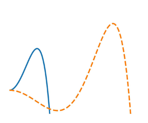
Figure 1 shows the growth rate (3.5) for two sets of dynamo numbers. We see that depending on the parameters, the growth rate may peak at large scales or at small scales.

Figure 1. The mode growth rate ($T\operatorname {Re}(\lambda )$, (3.5)) as a function of the wavenumber for two combinations of $\mathcal {D}_1$ and $\mathcal {D}_2$.

To understand the qualitative behaviour of (3.5), we can schematically write it as

(3.6)\begin{equation} \operatorname{Re}(\lambda) =\begin{cases} - k^2 - k^4 - k^6 - k^8 ; & \mathcal{D}_2 > 1,\, \mathcal{D}_1 < 1\\ - k^2 + k^4 - k^6 - k^8 ; & \mathcal{D}_2 < 1,\, \mathcal{D}_1 < 1 \\ k^2 + k^4 - k^6 - k^8 ; & \mathcal{D}_2 < 1,\, \mathcal{D}_1 > 1 \\ k^2 - k^4 - k^6 - k^8 ; & \mathcal{D}_2 > 1,\, \mathcal{D}_1 > 1. \end{cases} \end{equation}

In the first case, $\operatorname {Re}(\lambda )$ is always negative, and so there is no dynamo. In the last two cases, $\operatorname {Re}(\lambda )$ is positive for small $k$ and becomes negative for large wavenumbers. In the second regime, it seems to be difficult to say anything concrete (depending on the values of the coefficients, one can either have growth in a range of wavenumbers or growth nowhere).

Since (3.5) is a polynomial in $K$, one can easily solve for its extrema. In figure 2, we show the dynamo growth rate (where positive) and the wavenumber of the resulting large-scale field, as a function of $\mathcal {D}_1$ and $\mathcal {D}_2$.

Figure 2. (a) The peak growth rate ($T\operatorname {Re}(\lambda )$, (3.5)). In the white regions, the growth rate is negative for all $K$. (b) The wavenumber ($K$) at which the growth rate peaks. Recall that, for a mode with wavelength $l_c$, the wavenumber would be $K=2{\rm \pi} \approx 10^{0.8}$.

If we drop the terms of order $K^6$ and $K^8$ in (3.5) (this does not change the qualitative behaviour when $\mathcal {D}_2 > 1$), we can estimate that if $\mathcal {D}_1 > 1$, the growth rate attains a maximum value at $K_{peak}$, where

(3.7a,b)\begin{equation} K_{peak} \approx \sqrt{ \frac{9 \left(\mathcal{D}_1 - 1\right)}{8 \mathcal{D}_1 \left(\mathcal{D}_2-1\right)} } ,\quad \left[T \operatorname{Re}(\lambda) \right]_{max} \approx \frac{9 \left(\mathcal{D}_1 - 1\right)^{2}}{16 \mathcal{D}_1 \left(\mathcal{D}_2 - 1\right)}. \end{equation}

Broadly speaking, there are two kinds of regimes in which the dynamo is excited. One, $\mathcal {D}_1 > 1$, corresponds to the fluctuations being strong enough that the effective diffusivity itself becomes negative (but the growth itself is still cut off at small scales due to higher-order terms). The other, $\mathcal {D}_2 < 1$ (with $\mathcal {D}_1$ also $< 1$), corresponds to growth with the effective diffusion remaining positive; one can see, however, from figure 2 that this growth happens at smaller scales than in the other regime (but may still be at scales larger than $l_c$). While $\mathcal {D}_2 \ll 1$ can formally lead to growing solutions regardless of the value of $\mathcal {D}_1$, the growth then occurs at scales $\lesssim l_c$.

4. The effect of anisotropy

Although we have not done so in the above, it seems natural to assume that the temporal correlation function $S$, that appears in (2.10b), is even. This would allow one to take $\int _{-\infty }^\infty S(t) \, \mathrm {d} t = 1$ and define the correlation time of $\eta$ as $\tau _\eta \equiv \int _{-\infty }^\infty \left |t\right | S(t) \, \mathrm {d} t$.

Because $\mu$ is a scalar, assuming its double correlation is invariant under time reversal immediately implies $\tilde {Q}(\boldsymbol {k}) = \tilde {Q}(-\boldsymbol {k})$. We then conclude that

(4.1)\begin{equation} A^{(1)}_i = A^{(3)}_i = h(\boldsymbol{k}) = 0, \end{equation}

when the fluctuations of $\eta$ are separable, homogeneous, stationary and time-reversal invariant; this holds even without assuming that the fluctuations of $\eta$ are isotropic! We now study the dynamo assuming the double correlation of $\mu$ is time-reversal invariant and anisotropic.

Let us choose the coordinate axes $1,2,3$ to be along the principal axes of the matrix $\boldsymbol{\mathsf{A}}^{(2)}$ (defined in (2.20a–d)), with the corresponding eigenvalues being $-a_1$, $-a_2$ and $-a_3$ (such that $a_1 \geq a_3 \geq a_2$). By analogy with (3.4a–e), one can define the correlation length along each axis as $l_c^{(i)} \equiv \sqrt {A^{(0)}/a_i}$. It is physically reasonable to assume $Q(\boldsymbol {\xi })$ attains a local maximum at the origin, and that its correlation length is finite. This means $a_1, a_2, a_3 > 0$.

Analogous to (3.4a–e), we define

(4.2a–e)\begin{equation} \mathcal{D}_1 \equiv \frac{9 a_3}{8 \bar{\eta} } ,\quad \mathcal{D}_2 \equiv \frac{81 \tau_\eta a_3^2 }{32 A^{(0)} } ,\quad l_c \equiv \sqrt{ \frac{ A^{(0)} }{ a_3 } } ,\quad \boldsymbol{K} \equiv \boldsymbol{k} l_c ,\quad T \equiv \frac{l_c^2}{\bar{\eta} }. \end{equation}

We also define the new quantities

(4.3a–d)\begin{equation} \chi_1 \equiv \frac{a_1}{a_3} - 1 ,\quad \chi_2 \equiv 1 - \frac{a_2}{a_3} ,\quad n_1 \equiv \frac{ \left|K_1\right| }{K} ,\quad n_2 \equiv \frac{ \left|K_2\right| }{K}, \end{equation}

and a modified dynamo number

(4.4)\begin{equation} \tilde{\mathcal{D}}_1 \equiv \mathcal{D}_1\left[ 1 + \frac{\chi_1}{9} ( 2 + 3 n_1^2 ) - \frac{\chi_2}{9} ( 2 + 3 n_2^2 ) \right]. \end{equation}

Since $0 \leq \chi _2 < 1$, $0 \leq \chi _1 < \infty$ and $0 \leq n_1, n_2 \leq 1$, we find that $\tilde {\mathcal {D}}_1 > 0$. We write $g(\boldsymbol {k})$ (2.23) as

(4.5)\begin{equation} T g(\boldsymbol{k}) = \tilde{\mathcal{D}}_1 K^2 + \frac{4\mathcal{D}_1}{9} \, K^4 . \end{equation}

Noting that $\tau _\eta /T = 4\mathcal {D}_2/(9\mathcal {D}_1)$, one can substitute (4.5) in (2.32) to obtain the following expression for the growth rate:

(4.6)\begin{equation} T \operatorname{Re}(\lambda) = K^{2} (\tilde{\mathcal{D}}_1 - 1) + \frac{ 4\mathcal{D}_1 K^{4} }{9} \left(1 - \frac{\mathcal{D}_2 \tilde{\mathcal{D}}_1^{2} }{ \mathcal{D}_1^2 }\right) - \frac{32 \mathcal{D}_2 \tilde{\mathcal{D}}_1 K^{6}}{81} - \frac{64 \mathcal{D}_1 \mathcal{D}_2 K^{8}}{729} . \end{equation}

As expected, this reduces to (3.5) on setting $\tilde {\mathcal {D}}_1 = \mathcal {D}_1$. Replacing $\mathcal {D}_1 \to \tilde {\mathcal {D}}_1$ and $\mathcal {D}_2 \to \mathcal {D}_2 \tilde {\mathcal {D}}_1^{2}/\mathcal {D}_1^2$, our comments in § 3 on the qualitative behaviour of (3.5) also apply to this equation. Unlike in the isotropic case, the growth rate now depends on the direction of $\boldsymbol {K}$ through the direction cosines $n_1$ and $n_2$. Figure 3 shows the growth rate as a function of the wavenumber for various parameter values.

Figure 3. The mode growth rate ($T\operatorname {Re}(\lambda )$, (4.6)) as a function of the wavenumber. In all the cases, we have taken $\mathcal {D}_1 = 2$ and $\mathcal {D}_2 = 5$. Other parameters not mentioned in the legend have been set to zero.

5. Suppression of turbulent diffusion

Neglecting terms with more than two spatial derivatives of $\langle \boldsymbol {B} \rangle$, (2.31) can be written as

(5.1) \begin{align} \frac{\partial}{\partial t} \langle \tilde{\boldsymbol{B}}(\boldsymbol{k}) \rangle &={-} \bar{\eta} k^2 \langle \tilde{\boldsymbol{B}}(\boldsymbol{k}) \rangle - \frac{1}{8} ( 3 k_mk_n {\mathsf{A}}^{(2)}_{mn} + 2 k^2 {\mathsf{A}}^{(2)}_{mm} ) \langle \tilde{\boldsymbol{B}}(\boldsymbol{k}) \rangle\nonumber\\ &\quad + \frac{{\rm i}}{8} \, k_m A^{(3)}_m \langle \tilde{\boldsymbol{B}}(\boldsymbol{k}) \rangle + \frac{\tau_\eta }{64} \, k_m k_i A^{(3)}_m A^{(3)}_i \langle \tilde{\boldsymbol{B}}(\boldsymbol{k}) \rangle + O(k^3) . \end{align}

Following the reasoning used in § 4 for $\tilde {\mathcal {D}}_1$, one can see that the coefficient of $\langle \tilde {\boldsymbol {B}}(\boldsymbol {k}) \rangle$ in the second term above is always positive as long as the spatial correlation function of the $\eta$-fluctuations attains a maximum at zero separation; the turbulent diffusion is suppressed. This can be seen more clearly in (2.24), which assumes a particular form for the spatial correlation function. The third term just describes advection with an effective velocity $\boldsymbol {A}^{(3)}/8$, analogous to ‘Moffatt drift’ (Moffatt 1978, § 7.11). The fourth term can never be negative, and is non-zero only when the fluctuations of $\eta$ are anisotropic and not invariant under time reversal. As noted in § 3, the higher powers of $k$ neglected in (5.1) can cause growth of the large-scale magnetic field even when the effective diffusivity is positive. They also ensure that the growth rate becomes negative at small scales.

It may seem counter-intuitive that a dissipative term ($\eta$) at the mesoscale leads to a dynamo at larger scales. However, it must be noted that, in addition to dissipation, $\eta$ also contributes an effective advection term (usually referred to as ‘turbulent diamagnetism’; see (2.2)) when spatial variations at the mesoscale are properly accounted for. Heuristically, it seems possible to explain the suppression of turbulent diffusion by turbulent diamagnetism as follows: turbulent diamagnetism causes the magnetic field to be preferentially concentrated in regions where the turbulent diffusivity is minimal. The effective turbulent diffusivity acting on the magnetic field is then less than what would be inferred by taking an average over the entire system. See Silant'ev (1999, p. 49) for a more general explanation of reduced turbulent diffusion when two scattering mechanisms contribute to the diffusion process.

6. Estimates of the dynamo numbers

Unfortunately, fluctuations of the turbulent diffusivity in astrophysical systems are not sufficiently constrained by observations. The situation in the solar photosphere is comparatively better, as observations of granulation give us an idea of the order of magnitude of various quantities. To make crude estimates, we use (A1a,b), which assumes a specific form for the correlation function of $\eta$.

Let us assume $l_c = {3}\ {\rm Mm}$ (peak of the granulation's power spectrum as observed by Roudier & Muller 1986, figure 2) and $\tau _\eta = {400}\ {\rm s}$ (granule lifetime measured by Bahng & Schwarzschild 1961). The turbulent diffusivity in the photosphere is a scale-dependent quantity, which is moreover not very well constrained (Abramenko et al. 2011, figure 10). For the length scales of interest, it is not unreasonable to take $\bar {\eta } = {600}\ {\rm km}^2\ {\rm s}^{{-1}}$. Let us also assume $f=0.1$ ($\,f \equiv \langle \mu ^2\rangle /\bar {\eta }^2$). We then find $\mathcal {D}_1 \approx 6\times 10^{-3}$ and $\mathcal {D}_2 \approx 4\times 10^{-4}$. These estimates appear to rule out the operation of such a dynamo in the solar photosphere. However, we note that assuming slightly different values of $l_c$ and $\tau _\eta$ brings the dynamo numbers to within the regime where a large-scale field can be generated; for example, taking $l_c = {300}\ {\rm km}$ and $\tau _\eta = {900}\ {\rm s}$ gives us $\mathcal {D}_1 \approx 1.4$ and $\mathcal {D}_2 \approx 18$. The dynamo numbers are also affected by uncertainties in $f$. Further, anisotropy can have a significant effect on the growth rates. Better estimates of the dynamo numbers would require measurements of the spatio-temporal correlation and strength of fluctuations of the turbulent diffusivity (or the kinetic energy) in the solar photosphere.

7. Conclusions

We have used a double-averaging procedure and found that just like helicity fluctuations, fluctuations of the turbulent kinetic energy can drive the growth of a large-scale magnetic field. While Silant'ev (1999, p. 49) has also reported that spatio-temporal fluctuations of the turbulent kinetic energy reduce the effective turbulent diffusion, we are not aware of any detailed studies of this effect that consistently account for the concomitant spatial gradients.

In the white-noise limit, we have found that $\eta$-fluctuations cause a reduction in the overall turbulent diffusion (in agreement with previous work), while also contributing a drift term which does not affect the growth of the field. We have then explored effects of non-zero correlation times and found the possibility of growing mean-field solutions despite the overall turbulent diffusion remaining positive. When the fluctuations are isotropic, the growth rate of a particular Fourier mode of the large-scale magnetic field depends on the magnitude of its wavevector and on two dynamo numbers. Anisotropy leads to a dependence on, among other things, the direction of the wavevector.

We have studied the conditions under which this new dynamo can operate. However, the lack of precise estimates of the quantities involved makes it hard to conclusively rule out or support the resulting dynamo in various astrophysical scenarios.

Given the prevalence of shear in astrophysical systems, an obvious extension of the current work would be to study the implications, for a large-scale magnetic field, of fluctuations of the turbulent kinetic energy in a shearing background. Since inhomogeneities in the density and in the small-scale magnetic energy also give rise to pumping (Vainshtein & Kichatinov 1983), we expect them to have effects similar to those described here.

References

Abramenko, V.I., Carbone, V., Yurchyshyn, V., Goode, P.R., Stein, R.F., Lepreti, F., Capparelli, V. & Vecchio, A. 2011 Turbulent diffusion in the photosphere as derived from photospheric bright point motion. Astrophys. J. 743 (2), 133.CrossRefGoogle Scholar
Bahng, J. & Schwarzschild, M. 1961 Lifetime of solar granules. Astrophys. J. 134, 312323.CrossRefGoogle Scholar
Brandenburg, A., Rädler, K.-H., Rheinhardt, M. & Käpylä, P.J. 2008 Magnetic diffusivity tensor and dynamo effects in rotating and shearing turbulence. Astrophys. J. 676 (1), 740751.CrossRefGoogle Scholar
Brandenburg, A. & Subramanian, K. 2005 Astrophysical magnetic fields and nonlinear dynamo theory. Phys. Rep. 417 (1–4), 1209.CrossRefGoogle Scholar
Busse, F.H. & Wicht, J. 1992 A simple dynamo caused by conductivity variations. Geophys. Astrophys. Fluid Dyn. 64 (1–4), 135144.CrossRefGoogle Scholar
Giesecke, A., Nore, C., Stefani, F., Gerbeth, G., Léorat, J., Luddens, F. & Guermond, J.-L. 2010 Electromagnetic induction in non-uniform domains. Geophys. Astrophys. Fluid Dyn. 104 (5–6), 505529.CrossRefGoogle Scholar
Gressel, O., Rüdiger, G. & Elstner, D. 2023 Alpha tensor and dynamo excitation in turbulent fluids with anisotropic conductivity fluctuations. Astron. Nachr. 344 (3), e210039. https://onlinelibrary.wiley.com/doi/pdf/10.1002/asna.20210039.CrossRefGoogle Scholar
Harris, C.R., et al. 2020 Array programming with NumPy. Nature 585 (7825), 357362.CrossRefGoogle ScholarPubMed
Hunter, J.D. 2007 Matplotlib: a 2d graphics environment. Comput. Sci. Engng 9 (3), 9095.CrossRefGoogle Scholar
Jones, C.A. 2011 Planetary magnetic fields and fluid dynamos. Annu. Rev. Fluid Mech. 43 (1), 583614.CrossRefGoogle Scholar
Knobloch, E. 1977 The diffusion of scalar and vector fields by homogeneous stationary turbulence. J. Fluid Mech. 83 (1), 129140.CrossRefGoogle Scholar
Kraichnan, R.H. 1976 Diffusion of weak magnetic fields by isotropic turbulence. J. Fluid Mech. 75 (part 4), 657676.CrossRefGoogle Scholar
Kraichnan, R.H. 1977 Eulerian and Lagrangian renormalization in turbulence theory. J. Fluid Mech. 83 (2), 349374.CrossRefGoogle Scholar
Krause, F. & Rädler, K.-H. 1980 Mean-Field Magnetohydrodynamics and Dynamo Theory, 1st edn. Pergamon.Google Scholar
Moffatt, H.K. 1978 Magnetic Field Generation in Electrically Conducting Fluids. Cambridge University Press.Google Scholar
Moffatt, H.K. 1983 Transport effects associated with turbulence with particular attention to the influence of helicity. Rep. Prog. Phys. 46 (5), 621664.CrossRefGoogle Scholar
Monin, A.S. & Yaglom, A.M. 1971 Statistical Fluid Mechanics: Mechanics of Turbulence, vol. 1. MIT.Google Scholar
Monin, A.S. & Yaglom, A.M. 1975 Statistical Fluid Mechanics: Mechanics of Turbulence, vol. 2. MIT.Google Scholar
Nicklaus, B. & Stix, M. 1988 Corrections to first order smoothing in mean-field electrodynamics. Geophys. Astrophys. Fluid Dyn. 43 (2), 149166.CrossRefGoogle Scholar
Pouquet, A., Frisch, U. & Léorat, J. 1976 Strong MHD helical turbulence and the nonlinear dynamo effect. J. Fluid Mech. 77 (2), 321354.CrossRefGoogle Scholar
Pétrélis, F., Alexakis, A. & Gissinger, C. 2016 Fluctuations of electrical conductivity: a new source for astrophysical magnetic fields. Phys. Rev. Lett. 116, 161102.CrossRefGoogle ScholarPubMed
Rincon, F. 2019 Dynamo theories. J. Plasma Phys. 85 (4), 205850401.CrossRefGoogle Scholar
Rincon, F. & Rieutord, M. 2018 The Sun's supergranulation. Living Rev. Solar Phys. 15 (1), 6.CrossRefGoogle Scholar
Roberts, P.H. & Soward, A.M. 1975 A unified approach to mean field electrodynamics. Astron. Nachr. 296 (2), 4964.CrossRefGoogle Scholar
Rogers, T.M. & McElwaine, J.N. 2017 The hottest hot jupiters may host atmospheric dynamos. Astrophys. J. Lett. 841 (2), L26.CrossRefGoogle Scholar
Roudier, Th. & Muller, R. 1986 Structure of the solar granulation. Sol. Phys. 107 (1), 1126.CrossRefGoogle Scholar
Ruzmaikin, A.A., Shukurov, A.M. & Sokoloff, D.D. 1988 Magnetic Fields of Galaxies, Astrophysics and Space Science Library, vol. 113. Kluwer Academic Publishers.CrossRefGoogle Scholar
Rädler, K.-H., Kleeorin, N. & Rogachevskii, I. 2003 The mean electromotive force for MHD turbulence: the case of a weak mean magnetic field and slow rotation. Geophys. Astrophys. Fluid Dyn. 97 (3), 249274.CrossRefGoogle Scholar
Silant'ev, N.A. 1999 Large-scale amplification of a magnetic field by turbulent helicity fluctuations. J. Expl Theor. Phys. 89, 4555.CrossRefGoogle Scholar
Silant'ev, N.A. 2000 Magnetic dynamo due to turbulent helicity fluctuations. Astron. Astrophys. 364, 339347.Google Scholar
Singh, N.K. 2016 Moffatt-drift-driven large-scale dynamo due to $\alpha$ fluctuations with non-zero correlation times. J. Fluid Mech. 798, 696716.CrossRefGoogle Scholar
Singh, N.K. & Jingade, N. 2015 Numerical studies of dynamo action in a turbulent shear flow. I. Astrophys. J. 806 (1), 118.CrossRefGoogle Scholar
Sokolov, D.D. 1997 The disk dynamo with fluctuating spirality. Astron. Rep. 41 (1), 6872.Google Scholar
Sridhar, S. & Singh, N.K. 2014 Large-scale dynamo action due to ${\alpha }$ fluctuations in a linear shear flow. Mon. Not. R. Astron. Soc. 445 (4), 37703787.CrossRefGoogle Scholar
Vainshtein, S.I. & Kichatinov, L.L. 1983 The macroscopic magnetohydrodynamics of inhomogeneously turbulent cosmic plasmas. Geophys. Astrophys. Fluid Dyn. 24 (4), 273298.CrossRefGoogle Scholar
Vishniac, E.T. & Brandenburg, A. 1997 An incoherent ${\alpha }-{\varOmega }$ dynamo in accretion disks. Astrophys. J. 475 (1), 263274.CrossRefGoogle Scholar
Yousef, T.A., Heinemann, T., Schekochihin, A.A., Kleeorin, N., Rogachevskii, I., Iskakov, A.B., Cowley, S.C. & McWilliams, J.C. 2008 Generation of magnetic field by combined action of turbulence and shear. Phys. Rev. Lett. 100, 184501.CrossRefGoogle ScholarPubMed