Measurement and analysis of sub-convective wall pressure fluctuations in turbulent boundary layer flows

Abstract

Sub-convective wall pressure fluctuations play a critical role in vibroacoustic and noise analyses of vehicle structures as they serve as the primary forcing function. However, measuring these fluctuations is challenging due to their weak pressure magnitudes, typically $10^{-3}{-}10^{-5}$ of convective fluctuations. This study introduces a non-intrusive measurement technique using an array of multi-pore Helmholtz resonator sensors to capture sub-convective fluctuations with high resolution. The array features large-area, spanwise-oriented sensors arranged linearly for optimal sampling. Results provide a continuous streamwise wavenumber–frequency spectrum, resolving sub-convective fluctuations with sufficient range and accuracy. Convergence analysis indicates that long sampling durations, $\mathcal{O}(10^6 \delta ^*/U_\infty )$, $\delta^*$ is the displacement thickness of the boundary layer. $U_\infty$ is the freestream velocity are necessary to capture true sub-convective levels. Comparisons with four existing wall pressure models, which account for sensor area averaging, reveal discrepancies in predicted levels, convection speed relations and convective ridge characteristics. Notably, the measured data align most closely with the Chase (1980, J. Sound Vib., vol.70, pp. 29–67) model at convective peak levels and in the sub-convective domain. However, the observed roll-off at wavenumbers exceeding the convective wavenumber decays more slowly than predicted, giving the convective ridge an asymmetric profile about the convective line. These findings underscore the need for improved wall pressure models that incorporate frequency-dependent convective speed relations, ridge asymmetry, and more accurate sub-convective levels. Further validation using a microphone array from Farabee & Geib (1991) confirms the accuracy of our measurements, which indicate sub-convective pressure levels lower than reported previously.

1. Introduction

The interaction of a solid surface with a fluid generates a thin region of influence at the wall responsible for momentum transfer, heat transfer and noise. This region is referred to as a boundary layer, and the practical importance of these layers is in the prediction of drag, heat transfer and radiated noise, especially in turbulent flow conditions. Studying the footprint of turbulent boundary layers on a surface can lead to a fundamental understanding of wall-bounded turbulence due to their coupling with the velocity field given by the pressure Poisson equation (Butt et al. 2024c ). Pressure fluctuations associated with turbulent boundary layers have been studied for over 50 years. They are well documented in the form of the two-point space–time correlations and wavenumber–frequency spectrum. Figure 1 shows a schematic of the wall pressure spectrum for an equilibrium two-dimensional turbulent boundary layer that is classified into three regions: (i) convective ridge (around the red dashed line), (ii) supersonic/acoustic (encompassed in a cone shown by black dashed lines), and (iii) sub-convective as shown. The axes represent the streamwise wavenumber ( $k_1$ ), spanwise wavenumber ( $k_3$ ) and frequency. Pressure fluctuations generated directly by the footprint of convecting turbulent eddies are located primarily in the convective ridge, characterised by a slope (in streamwise wavenumber $k_1$ and frequency) equal to the average convection speed of the eddies, typically between 60 % and 80 % of the boundary layer edge velocity. Grazing sound waves form an acoustic cone with a surface slope equal to the sound speed, while all other sound waves appear within the cone due to their supersonic trace velocity across the wall. This is known as the supersonic region of the spectrum. The boundary layer also produces weak pressure fluctuations at wavenumber–frequency combinations in the sub-convective domain, which is the three-dimensional region between the acoustic cone and the convective ridge. This region is practically relevant in vehicle noise due to its coupling to the fundamental vibration modes of a rigid or semi-rigid surface. These fluctuations are presumably associated with elongated turbulent structures, non-sinusoidal components of convected eddies, and near-field sound waves generated within the turbulence, and scattered from any non-planar features of the surface. However, there has been no clear evidence to claim the sources of these pressure fluctuations, and these presumed sources are based on certain hypotheses and scaling arguments. Recently, Butt et al. (2024b ) showed pressure–velocity correlations in the form of the wavenumber–frequency spectrum, highlighting the relevance of all three velocity components to convective wall pressure. Butt (2025) performs additional analysis on correlating wall pressure with Reynolds stresses ( $\phi _{pu_1u_1}, \phi _{pu_1u_2}$ ), highlighting their plausible relevance in sub-convective contributions.

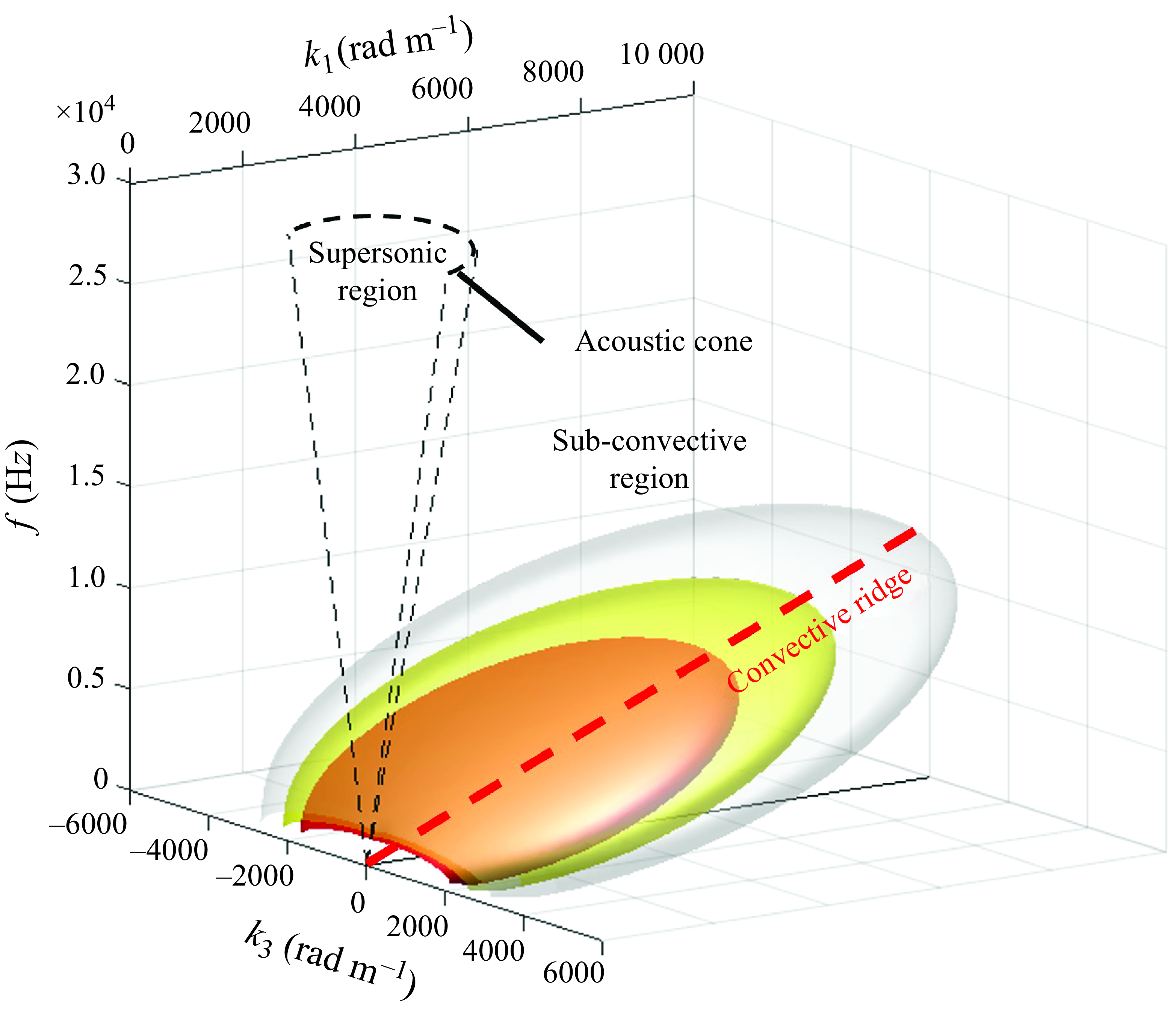
Figure 1. Schematic of the wall pressure wavevector–frequency spectrum (Glegg & Devenport 2024).

There are challenges associated with measurements in the sub-convective region, mainly due to the weak magnitudes of pressure fluctuations, which are easily masked by the convective fluctuations and the scales associated with these fluctuations. Performing a wall pressure measurement using a single pressure transducer yields a frequency spectrum that does not distinguish between the three regions. To study the regions separately, two-point measurements are needed, which comes with challenges when measuring the wavenumber–frequency combinations in the sub-convective domain. At least three techniques have been attempted to separate pressure field components from the intense fluctuations associated with the convective ridge. One approach, pioneered by Maidanik & Jorgensen (1967) and further developed by Blake & Chase (1970), Farabee & Geib (1991) and Kudashev (2007), uses a regularly spaced array of large-area pressure fluctuation sensors. This technique utilised the convective pressure averaging of the large-area sensors and wave-vector filtering by selectively phasing the signals. This filtering achieved high sensitivity towards integral wavenumbers corresponding to the spacing between sensors, giving rise to measurements in the sub-convective and acoustic region of the spectrum. However, these measurements were highly selective, providing measurements at only a handful of wavenumber–frequency combinations. It was difficult to differentiate further if the levels had contamination from other components or suffered from spatial aliasing.

A second method for measuring low-wavenumber components of the wall pressure spectrum involves using a thin, flexible membrane excited by turbulent motions. Martin & Leehey (1977) studied a Mylar membrane under a plane wall boundary layer in air, Bonness, Capone & Hambric (2010) conducted measurements on a thin cylindrical aluminium shell to relate it to fluid excitation in a turbulent pipe flow, and Golubev (2012) examined thin aluminium alloy and glass plates under a planar turbulent boundary layer. The concept behind such measurements is an inversion problem that relates the flexible membranes’ structural modes to the wall pressure excitation. This theory works well at resolving wavenumbers corresponding to the resonance modes of the flexible membrane structure. However, its extension to more general flow scenarios, such as pressure gradient effects, surface roughness and inhomogeneity, is limited. Panel vibration measurements have provided a vast majority of low-wavenumber ( $0.8\lt \omega \delta ^* /U_c\lt 5$ ), $\omega$ is the angular frequency, $\delta^*$ is the displacement thickness and $U_c$ is the nominal convective speed, measurements of the surface pressure spectrum; however, they are limited by the flow condition, flexible membrane, and boundary conditions on the membrane.

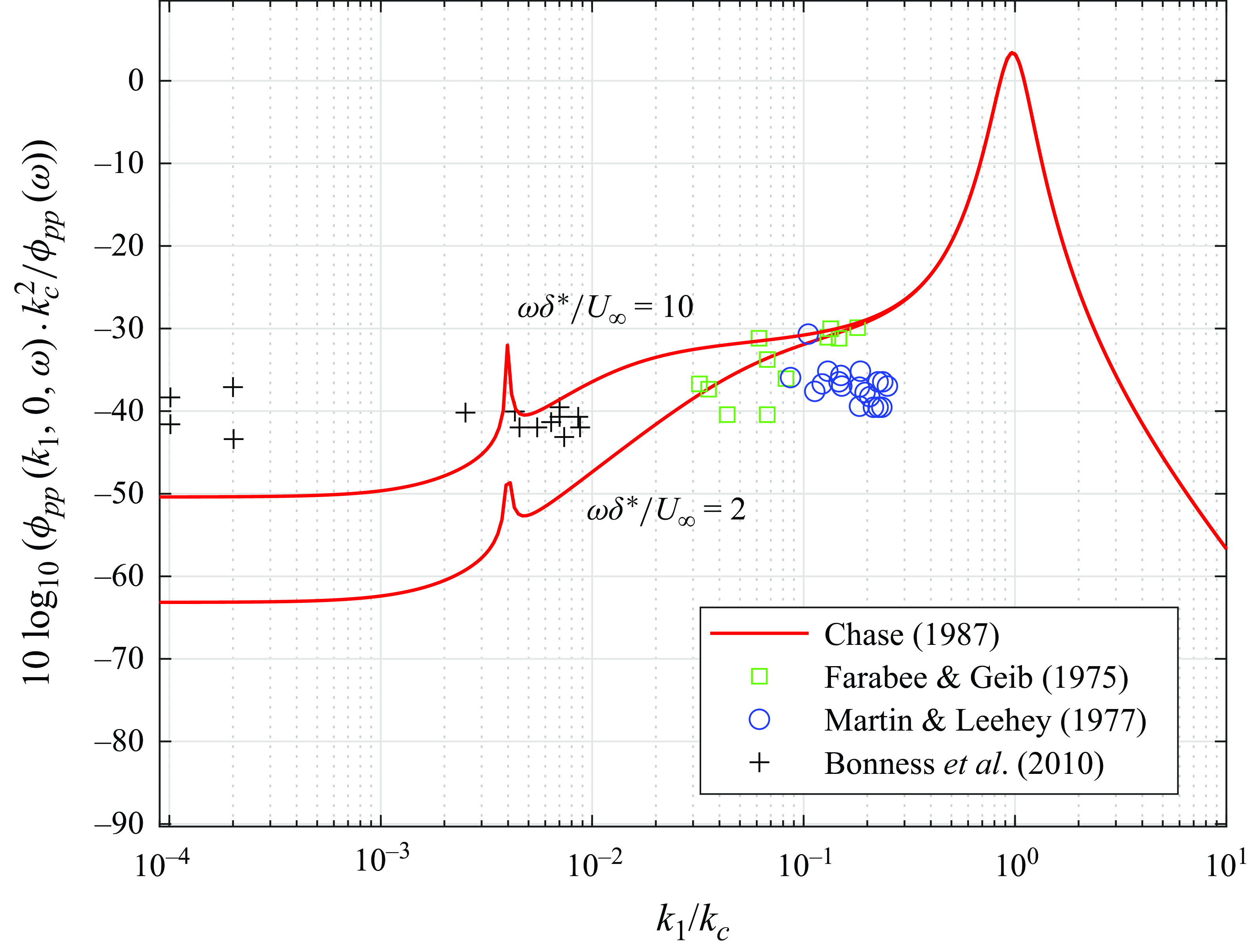
Figure 2. Comparison between the comprehensive compressible Chase model (Chase 1987) and previous experimental studies. Adapted from Blake (2017).

A third approach for measuring the wavenumber–frequency spectrum involves using large arrays of electret, remote or digital microphones that can resolve smaller turbulent scales. This method has been popular among researchers studying automobile wind noise, e.g. Arguillat et al. (2005). The arrangement of the microphones was optimised into ‘co-arrays’, and a deconvolution technique was used to back out the wavenumber–frequency spectrum (Ehrenfried & Koop 2008; Gabriel et al. 2013; Schram & Van de Wyer 2018). This large-array/small-sensor approach has produced maps revealing the convective ridge and acoustic cone. However, whether this strategy can effectively resolve the low spectral levels in the subsonic region away from the convective ridge remains uncertain. Recently, Prigent, Salze & Bailly (2022) showed measurements of the wavenumber–frequency spectrum obtained using an antenna comprising 63 non-uniformly distributed remote microphones inserted in a vinyl tube attachment. Comparisons with wall pressure models such as those of Corcos (1967) and Chase (1987) revealed agreements at the convective peak but deviations in the sub-convective regime, i.e. $k_1\lt k_c$ . The authors suggested insufficiency in using deconvolution techniques to resolve pressure fluctuations in the sub-convective regime. Furthermore, a recent study by Abtahi, Karimi & Maxit (2024b ) reiterated the need for a higher number of realisations (longer sampling duration) to resolve the gap between the sub-convective and convective levels. This poses another challenge, as the lower limit of the sub-convective levels is unknown.

A detailed review of the measurement techniques used to quantify sub-convective pressure fluctuations has been presented in Damani et al. (2022) and Abtahi et al. (2024b ). These works highlight the discrepancies between different studies due to the difference in flow across various facilities and the uncertainty due to the measurement technique. The techniques suffer mainly from spatial aliasing, poor signal-to-noise ratios, and the inability to apply to general flow regimes. Furthermore, no measurement approaches to date have been able to provide continuous measurement of the sub-convective pressure as a function of wavenumber and frequency. This makes it challenging to validate wall pressure models in the sub-convective domain due to limitations in flow data. Figure 2 presents a comparison from Blake (2017) of the wavenumber–frequency spectrum predicted by the Chase model (Chase 1987) at two frequencies ( $\omega \delta ^*/U_\infty =2, 10$ ) against experimental data from various studies. The plot contains approximately 40 discrete data points from four studies representing most of the accepted sub-convective pressure measurements, showing a limited wavenumber range resolved by each study.

In recent years, there have been attempts to generalise the wall pressure models in terms of their space–time correlations and wavenumber–frequency spectrum by accommodating pressure gradient effects and frequency-dependent convective relations. It is important to note that many of these studies focus purely on the frequency spectrum, which is not sufficient to study the sub-convective domain. Studies such as Hu & Herr (2016) and Hu (2021) quantified the dependence of the wall pressure levels, coherence length scales and convective energy using small microphones under various flow regimes, including pressure gradients. Caiazzo et al. (2016) extended the Corcos model (Corcos 1967) to a generalised form using a two-dimensional Butterworth filter, which helped to reduce the sub-convective regime’s levels. Hwang, Bonness & Hambric (2003) and Smol’yakov (2006) used mixed correlation length scales to accommodate lower sub-convective levels. Recently, Frendi & Zhang (2020) recommended a semi-empirical model based on modifications to the Corcos (1967) and Efimtsov (1982) models to improve the shape and spectral levels in the sub-convective regime.

Also in recent years, there have been developments in wall pressure sensing technology, with Damani et al. (2025) demonstrating the use of Kevlar-covered sensors under turbulent boundary layers. These sensors possess convective pressure averaging capabilities and flexibility in manufacturing. However, the study concludes that a Kevlar interface makes it challenging to predict the averaging, and alternatives are sought. The study presented here introduces an alternative approach to selectively filter convective pressure fluctuations with the overall objective of measuring the sub-convective wall pressure fluctuations. It uses an array of custom-built sensors based on multi-pore Helmholtz resonators that are non-intrusive to the overlying flow. High-quality microphones with a large dynamic range are employed to measure the weak sub-convective pressure fluctuations with high signal-to-noise ratios. This measurement approach reveals, for the first time, the continuous form of the sub-convective pressure spectrum in a high Reynolds number turbulent boundary layer. The measurements are compared against existing wall pressure models.

Section 2 presents a review of wall pressure models used for comparison. Section 3 outlines the method for accounting for area averaging by assuming a lumped system model for the sensors, and presents results for the array configuration used in this study. Section 4 describes the flow conditions, sub-resonant sensor array, and calibration. Section 5 presents a detailed description of the results and their comparison with models of the cross-spectrum and wavenumber–frequency spectrum. The results showcase a continuous wavenumber–frequency spectrum with sufficient range and resolution in the sub-convective regime. Comparisons with wall pressure models show promising agreement with the incompressible Chase (1980) model, providing the most detailed validation and assessment of this model to date.

2. Review of wall pressure models

Four well-known wall pressure models were chosen for comparison with acquired data. The following subsections describe each model with a form for its space–frequency cross-spectral density function and the resulting wavenumber–frequency spectrum.

2.1. Corcos

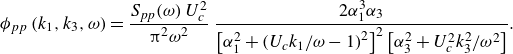
The Corcos (1967) model is widely used for the wall pressure spectrum due to its mathematical form, which separates the correlations in streamwise and spanwise directions. In its original form, this model defines the wavenumber–frequency spectrum ( $\phi _{pp}$ ) as

(2.1) \begin{equation} \phi _{pp}(k_1, k_3, \omega ) = \frac {S_{pp}(\omega )\, U_c^2}{\unicode{x03C0} ^2 \omega ^2} \frac {\alpha _1 \alpha _3}{\left[\alpha _1^2 + (U_c k_1/\omega -1)^2\right]\left[\alpha _3^2 + U_c^2 k_3^2/\omega ^2\right]}, \end{equation}

where $S_{pp}(\omega )$ is the single-point wall pressure spectrum evaluated using a separate model such as Goody (2004), $U_c$ is the convective speed of the turbulence, and $\alpha _{1,3}$ are empirical constants usually defined as 0.1 and 0.77, respectively. The same model in the space–frequency domain in terms of cross-spectral density ( $\Gamma$ ), normalised on the autospectrum, is given by

(2.2) \begin{equation} \Gamma (\Delta x_1, \Delta x_3, \omega ) = \textrm{e}^{\textrm{i} \frac {\omega }{U_c}\Delta x_1}\, \textrm{e}^{-\alpha _1 \frac {\omega }{U_c}|\Delta x_1|}\, \textrm{e}^{-\alpha _3 \frac {\omega }{U_c}|\Delta x_3|}. \end{equation}

This model is well suited for the convective domain; however, it is believed to overpredict the sub-convective spectrum, especially at low wavenumbers. There has been work on modifying the original Corcos model to account for the overprediction at lower wavenumbers, which has given rise to various other forms of the Corcos model, such as those described by Smol’yakov (2006) and Caiazzo et al. (2016).

2.2. Incompressible Chase

The incompressible Chase model (Chase 1980) and its compressible counterpart (Chase 1987) differ primarily in their spectral predictions within the acoustic cone, a region outside the wavenumber range of primary interest in this study. Given that the incompressible formulation provides a convenient closed-form analytical expression for the cross-spectrum, it is adopted for the present analysis. The wall pressure spectrum from Chase (1980) is given by

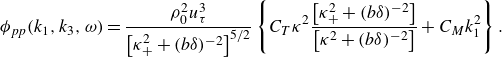(2.3) \begin{equation} \phi _{pp}(k_1, k_3, \omega ) = \frac {\rho _0^2 u_{\tau }^3}{\left[\kappa _+^2+(b\delta )^{-2} \right]^{5/2}} \left \{ C_T \kappa ^2 \frac {\left[\kappa _+^2+(b\delta )^{-2} \right]}{\left[\kappa ^2+(b\delta )^{-2} \right]} + C_M k_1^2 \right \}. \end{equation}

Some constants used in the model are $C_T=0.014/h,\ h=3,\ C_M=0.466/h, b=0.75,\ c_2 =c_3=1/6$ . Some other variables are defined as

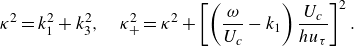(2.4) \begin{align} \kappa ^2 = k_1^2+k_3^2,\quad \kappa _+^2 = \kappa ^2 + \left [ \left ( \frac {\omega }{U_c}-k_1 \right ) \frac {U_c}{hu_{\tau }} \right ]^2. \end{align}

The model is considered to be the most accurate due to its derivation from first principles. According to the authors’ knowledge, no work has a sufficient wavenumber range and resolution to provide detailed validation of this model, specifically in the sub-convective domain. The cross-spectral density function ( $\Gamma$ ) is given by

(2.5) \begin{align} \Gamma (\Delta x_1, \Delta x_3, \omega ) &= a_+\tau _w^2\omega ^{-1}\,\textrm{e}^{\textrm{i}\omega\, \Delta x_1/U_c}\,\textrm{e}^{-\zeta }[r_M\,f_M(\Delta x_1, \Delta x_3,\omega ) \nonumber \\&\quad + r_T\,f_T(\Delta x_1, \Delta x_3,\omega )], \end{align}

where the variables are defined as

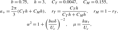(2.6) \begin{gather} b=0.75, \quad h=3, \quad C_T=0.0047, \quad C_M=0.155,\nonumber \\ a_+ = \frac {2\unicode{x03C0} }{3}(C_Th+C_Mh), \quad r_T = \frac {C_Th}{C_Th + C_Mh}, \quad r_M=1-r_T,\nonumber \\ \alpha ^2 = 1 + \left (\frac {b\omega \delta }{U_c}\right )^{-2}, \quad \mu =\frac {hu_{\tau }}{U_c},\end{gather}

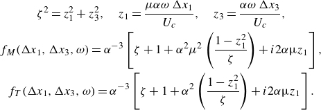(2.7) \begin{gather} \zeta ^2 = z_1^2+z_3^2, \quad z_1 = \frac {\mu \alpha \omega\, \Delta x_1}{U_c}, \quad z_3 = \frac {\alpha \omega\, \Delta x_3}{U_c},\nonumber \\f_M(\Delta x_1, \Delta x_3,\omega ) = \alpha ^{-3} \left [ \zeta + 1 + \alpha ^2 \mu ^2 \left (\frac {1-z_1^2}{\zeta }\right ) + i2\alpha \unicode{x03BC} z_1 \right ],\nonumber \\f_T(\Delta x_1, \Delta x_3,\omega ) = \alpha ^{-3} \left [ \zeta + 1 + \alpha ^2 \left (\frac {1-z_1^2}{\zeta }\right ) + i2\alpha \unicode{x03BC} z_1 \right ]. \end{gather}

The autospectral density for this model is described by

(2.8) \begin{equation} S_{pp}(\omega ) = a_+\tau _w^2\omega ^{-1} \alpha ^{-3}\bigr[r_M + r_M\mu ^2\alpha ^2 + r_T + r_T\alpha ^2\bigr]. \end{equation}

2.3. Modified Corcos

A modification to the Corcos model was suggested by Hwang et al. (2003). This model is known to approximately achieve sub-convective levels similar to the Chase models. The wavenumber–frequency form of the model is given by

(2.9) \begin{equation} \phi _{pp}\left (k_1,k_3,\omega \right ) = \frac {S_{pp} (\omega )\,U_c^2}{\unicode{x03C0} ^2\omega ^2}\ \frac {2\alpha _1^3\alpha _3}{\left [\alpha _1^2+\left (U_ck_1/\omega -1\right )^2\right ]^2\left [\alpha _3^2+U_c^2k_3^2/\omega ^2\right ]}. \end{equation}

The cross-spectral density ( $\Gamma$ ), normalised on the autospectrum, is defined as

(2.10) \begin{equation} \Gamma (\Delta x_1, \Delta x_3, \omega ) = \Big (1 + \alpha _1 \frac {\omega }{U_c}\,|\Delta x_1| \Big ) \textrm{e}^{\textrm{i} \frac {\omega }{U_c}\Delta x_1}\, \textrm{e}^{-\alpha _1 \frac {\omega }{U_c}|\Delta x_1|}\, \textrm{e}^{-\alpha _3 \frac {\omega }{U_c}|\Delta x_3|}. \end{equation}

Since the modified Corcos model replicates the low sub-convective levels of the Chase spectrum but in an algebraically simpler form, we will use it later in the paper to model the measurement process and estimate measurement errors.

2.4. Smol’yakov

Smol’yakov (2006) developed a model using measurements with a slightly different approach. Instead of separating the longitudinal and lateral separations, these were combined into an oblique spatial separation term. The resulting low-wavenumber levels were generally lower than those of the Corcos model. The wavenumber–frequency spectrum is given by

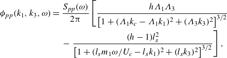(2.11) \begin{align} \phi _{pp}(k_1, k_3, \omega ) ={}& \frac {S_{pp}(\omega )}{2\unicode{x03C0} } \left [ \frac {h\Lambda _1\Lambda _3}{\left[1 + (\Lambda _1k_c - \Lambda _1k_1)^2 + (\Lambda _3k_3)^2\right]^{3/2}}\right. \\ &{}-\left . \frac {(h-1)l_s^2}{\left[1+ (l_sm_1\omega /U_c-l_sk_1)^2 + (l_sk_3)^2\right]^{3/2}} \right ],\nonumber \end{align}

where the terms are defined as

(2.12) \begin{align}&\qquad\qquad\quad m_0 = 6.45, \quad n = 1.005, \end{align}

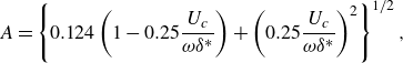(2.13) \begin{align}& A = \left \{ 0.124 \left ( 1-0.25\frac {U_c}{\omega \delta ^*}\right ) + \left ( 0.25\frac {U_c}{\omega \delta ^*} \right )^2 \right \}^{1/2}, \end{align}

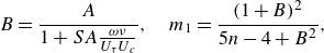(2.14) \begin{align}&\quad B = \frac {A}{1+SA \frac{\omega \nu }{U_{\tau } U_c}}, \quad m_1 = \frac {(1+B)^2}{5n-4+B^2}, \end{align}

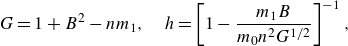(2.15) \begin{align}&\quad\,\, G = 1+B^2-nm_1, \quad h = \left [ 1 - \frac {m_1B}{m_0n^2G^{1/2}} \right ]^{-1}, \end{align}

(2.16) \begin{align}& \Lambda _1 = \frac {U_c}{B\omega }, \quad \Lambda _3 = \frac {U_c}{m_0B\omega }, \quad l_s = \left (\frac {U_c}{\omega }\right )\left [\frac {n}{m_1G}\right ]^{1/2}, \end{align}

with $S$ having a value between 0 and 100. The form for the cross-spectral density ( $\Gamma$ ), normalised on the autospectrum, is given by

(2.17) \begin{equation} \Gamma (\Delta x_1, \Delta x_3, \omega ) = h\gamma\, \textrm{e}^{\textrm{i}\,\Delta x_1\,\omega /U_c} - (h-1)\,\Delta \gamma\, \textrm{e}^{\textrm{i} m_1\,\Delta x_1\, \omega /U_c}, \end{equation}

where $\gamma$ and $\Delta \gamma$ are defined as

(2.18) \begin{align} \gamma & = \textrm{e}^{-\left[\left(\Delta x_1/\Lambda _1\right)^2 + \left(\Delta x_3/\Lambda _3\right)^2\right]^{1/2}}, \nonumber\\ \Delta \gamma & = \textrm{e}^{-\left[\left(\Delta x_1/l_s\right)^2 + \left(\Delta x_3/l_s\right)^2\right]^{1/2}},\end{align}

which follow the same variable definitions as described earlier.

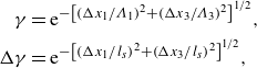
Figure 3 compares the above-described models at two frequencies when evaluated for boundary layer parameters shown in table 2. The horizontal axis represents the streamwise wavenumber ( $k_1$ ) normalised by the convective wavenumber ( $k_c=\omega /U_c$ ), while the vertical axis shows the normalised spectrum levels. All except the Chase model are classified as Corcos-type models due to their resemblance to the mathematical form of the Corcos model. The models show good agreement at convective wavenumbers, with only minor level differences. However, significant discrepancies are observed at sub-convective wavenumbers ( $k_1/k_c \lt 1$ ). The Chase model also shows some differences, but the modified Corcos and Smol’yakov models closely align with Chase’s predictions at higher sub-convective wavenumbers. All models exhibit some wavenumber-white behaviour in the sub-convective domain, consistent with Kraichnan (1956) criteria at higher frequencies. The wavenumber-white character breaks down at lower frequencies for the Chase model. Overall, all models show a large discrepancy at higher wavenumbers ( $k_1/k_c \gt 1$ ). The Smol’yakov model shows a broader convective peak, and the low-wavenumber levels are close to those of the modified Corcos model.

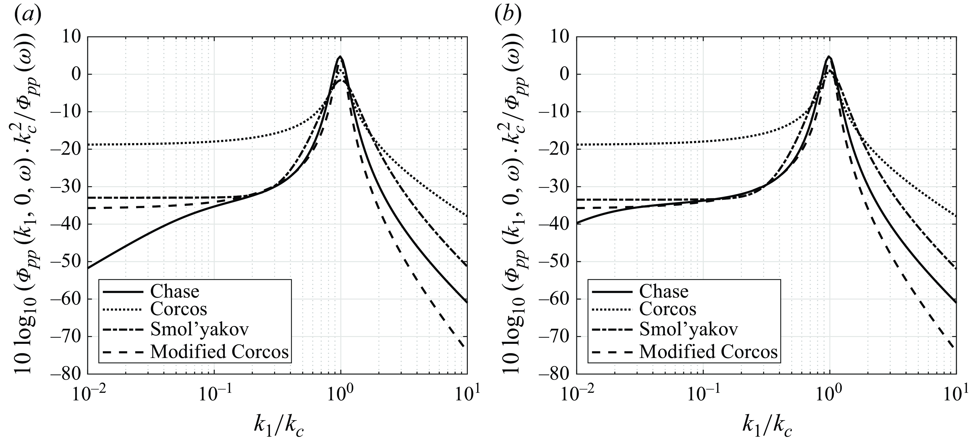
Figure 3. Comparison of zero spanwise wavenumber component of different models at frequencies (a) $\omega \delta ^*/U_e=2$ , (b) $\omega \delta ^*/U_e=10$ , as a function of streamwise wavenumber.

3. Designing an array of sub-resonant sensors for sub-convective pressure measurements

Area-averaged fluctuating wall pressures were measured using an array of 80 sub-resonant sensors, each comprised of an acoustic cavity, a microphone and a flow interface, as shown in figure 4(a). The development of these sensors is described in detail by Damani et al. (2024) and Damani (2025) and Damani et al. (2025). The sensors provide measurements at low frequencies where the cavities are too small, i.e. less than half an acoustic wavelength, for sound waves to exist within them. Surface pressure at the wall is communicated to the cavity through an array of small-diameter pores drilled through a thin, rigid cover or flow interface. Thus the sensor, comprising an acoustic cavity and pores, constitutes a multi-pore Helmholtz resonator. A key feature of these sensors in the present application is their large sensing area compared to the boundary-layer thickness (50 mm $\times$ 5 mm, $0.75\delta \times 0.075\delta$ ). This allows spatial averaging to filter out a significant fraction of the convective energy, improving the signal-to-noise ratio for the measurement of sub-convective pressure fluctuations.

Figure 4. (a) Individual sensor profile, with dimensions. (b) Placement of sensors and pores along the array (shaded rectangles represent individual sensors).

The sub-resonant sensors were 30 mm deep, tapering with depth to prevent interference between microphones of adjacent sensors, and allow sufficient wall rigidity. Each sensor featured 80 pores, each 0.4 mm in diameter and 1.1 mm deep. The pores were arranged in a uniform grid with 1.375 mm spacing along the flow direction, and 2.5 mm across, as determined by the analysis to be presented in $\S$ 3.4. Figure 4(b) shows a plan view of a short streamwise portion of the array (4 of 80 sensors), showing the relative placement of adjacent sensors. With 0.5 mm between the sensors in the streamwise direction, the pores of the sensors combine to make a uniform streamwise distribution. As discussed below, this minimised aliasing errors on the measurement of the surface pressure wavenumber–frequency spectrum.

The following subsections describe the methodology involved in optimising the design of the sub-resonant sensor array. They detail the assumptions and approximations needed to reduce a large design space, the derivation of a wavenumber–frequency spectrum relation for an array of linear sensors accounting for the sensor area averaging, and the assessment of error. The final sensor array geometry and estimates of its accuracy in the sub-convective range are then presented.

3.1. Basis for sensor design

The response of a sub-resonant sensor in the array (figure 4) can be approximated using a lumped system model. Langfeldt, Hoppen & Gleine (2019) demonstrated that the impedance of a multi-pore Helmholtz resonator can be expressed as the sum of individual neck impedances, and a similar approximation can be derived via momentum balance to relate the sensor response to cavity volume and pore geometry (Damani 2025). This approach assumes a linear response, independent of pore interactions.

Damani et al. (2025) used a localised source to study the pressure field over a sub-resonant (Kevlar-covered) sensor, and showed that the sensor exhibits area-averaging characteristics, with its pressure response reconstructable via a summation of monopole sources distributed over the pores. This confirms a linear relation between the external pressure above each pore and the cavity pressure, with further formulation details available in $\S$ 5.2 of Damani (2025).

Sensor resonance was found to increase with the number of pores (Langfeldt et al. 2019), and this linearity provides a practical foundation for performance assessment and error analysis. The negligible influence of these sensors on the overlying flow is supported by the findings of Léon et al. (2019), who reported no measurable flow disturbance from acoustic liners with pore sizes in the range $61\lt d^+={d}u_{\tau }/\nu \lt 261$ . The present study uses pore diameter $d^+=33.8$ , further ensuring minimal flow interference.

The spatial sensitivity function $\mathbb{A}$ may be represented as a linear summation of weighted Dirac delta functions:

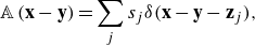(3.1) \begin{equation} \mathbb{A}\left (\mathbf{x}-\mathbf{y}\right )=\sum _{j} s_j\delta (\mathbf{x}-\mathbf{y}-\mathbf{z}_j), \end{equation}

where $\mathbf{x}$ denotes the sensor coordinate space defining its area, $\mathbf{z}_{{j}}$ gives the location of the $j$ th pore relative to the centre $\mathbf{y}$ of the sensor, and $s_j$ gives the relative sensitivity of the transducer to the pressure at each pore. Note that we must have

(3.2) \begin{equation} \sum _{j} s_j=1 \end{equation}

to preserve the scaling of the measured quantity. While the lumped approximation assumes uniform sensitivity ( $s_j=const$ ), experimental measurements and COMSOL simulations (see $\S$ 5.4.2 in Damani 2025) indicate sensitivity bias towards the deeper end of the sensor, where the microphone is located (figure 5). Although this bias decreases with frequency, it must be accounted for in high-resolution modelling and error evaluation. These sensitivity distributions are later incorporated into the design error analysis presented in $\S$ 3.4.

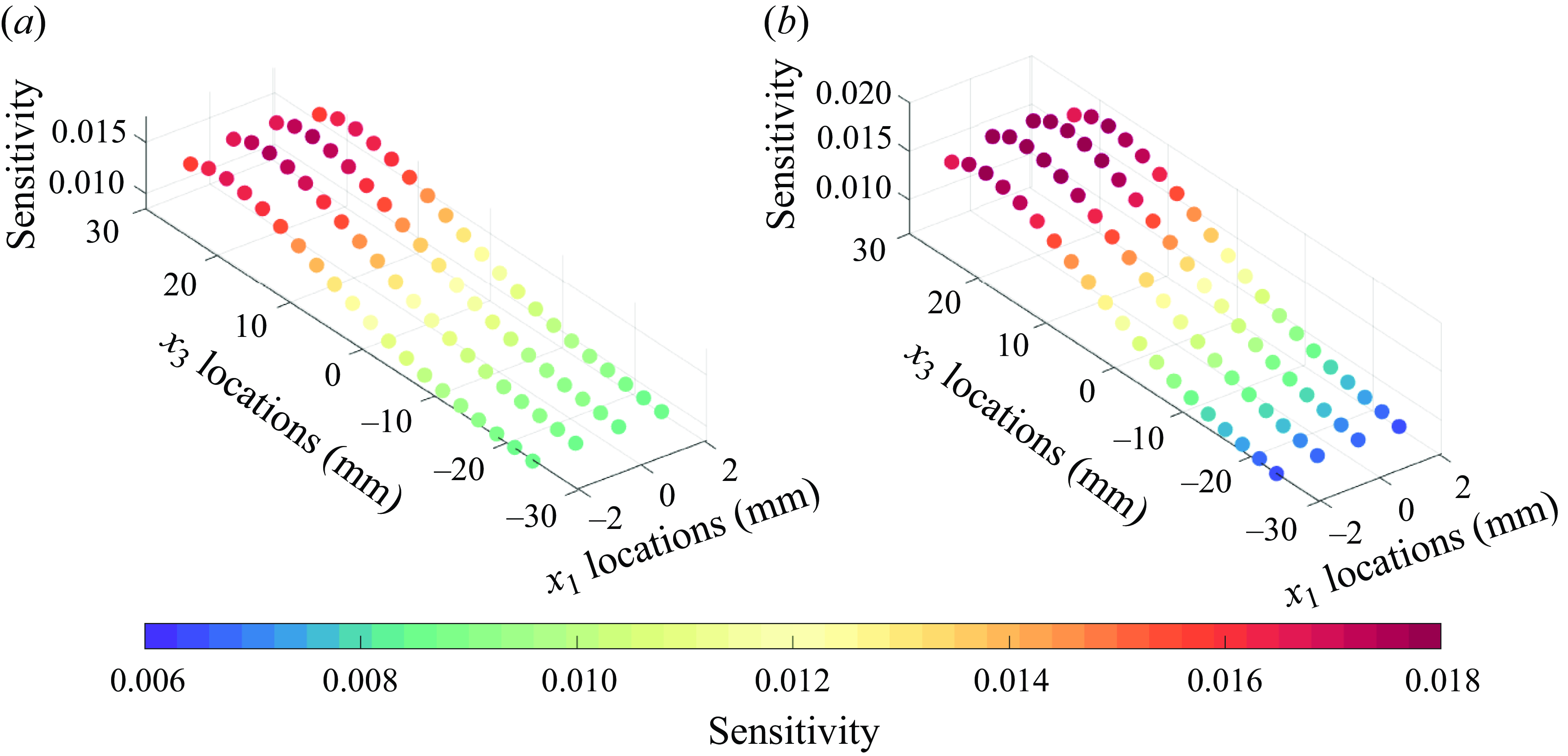
Figure 5. Sensitivity evaluated at each pore from COMSOL simulation for (a) $f=500$ Hz, (b) $f=1000$ Hz. The microphone centre was positioned 30 mm below $(x_1,x_3)=(0,21.5)$ .

3.2. Estimating wall pressure spectrum detected by the linear sensor array

To evaluate the likely accuracy of an array of the type shown in figure 4, we can use one of the model spectra from $\S$ 2 to estimate the wavenumber–frequency spectrum that the array would measure, and compare that back to the model to provide an estimate of the likely error. This process provides a means to assess the sensitivity of the errors to various design parameters, such as sensor surface area, pore distribution and sensor spacing, on the response variable. This works to optimise our design space within manufacturing and size constraints.

An estimate for the cross-spectral density function ( $S_{qq}(\Delta x_1,\omega)$ ) as measured by an array of sub-resonant sensors can be formulated based on a convolution between the true wall pressure and the sensor area sensitivity given by Blake & Chase (1970). This is represented using the equation

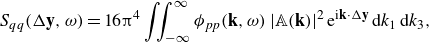(3.3) \begin{equation} S_{qq}(\Delta \mathbf{y}, \omega ) = 16\unicode{x03C0} ^4 \iint _{-\infty }^{\infty } \phi _{pp}(\mathbf{k},\omega )\,|\mathbb{A}(\mathbf{k})|^2\, \textrm{e}^{\textrm{i} \mathbf{k}\cdot\Delta \mathbf{y}}\, {\textrm d}k_1\, {\textrm d}k_3, \end{equation}

which uses the relation by White (1967) for an area-averaged wall pressure spectrum. Here, $\phi _{pp}$ is the wavenumber–frequency spectrum from a wall pressure model such as described in $\S$ 2, and $\mathbb{A}(\mathbf{k})$ is the wavenumber transform of the area sensitivity function. The exponential term ( $\textrm{e}^{\textrm{i} \mathbf{k}\cdot\Delta \mathbf{y}}$ ) is referred to as the array term, which accounts for the cross-correlation between different sensors distributed in space.

The wavenumber transform of the sensitivity function (3.1) is given by

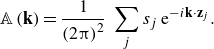(3.4) \begin{equation} \mathbb{A}\left (\mathbf{k}\right )=\frac {1}{\left (2\unicode{x03C0} \right )^2}\ \sum _{j} s_j\,\textrm{e}^{-i\mathbf{k}\cdot\mathbf{z}_j}. \end{equation}

Using this relation in (3.3), one can represent the cross-spectral density function as

(3.5) \begin{equation} S_{qq}(\Delta \mathbf{y}^{ (m,n )},\omega )=\sum _{N}\sum _{M}{{s_N^{(n )}}^\ast s_M^{(m)}}\,S_{pp}\left (\mathbf{y}^{\left (n\right )}+\mathbf{z}_N^{\left (n\right )}-\mathbf{y}^{\left (m\right )}-\textbf {z}_M^{\left (m\right )},\omega \right ), \end{equation}

where $n,m$ represent two different sensors, $N,M$ are the numbers of pores on each sensor, and $S_{pp}(\Delta \mathbf{y},\omega )$ refers to the pointwise cross-spectral density function evaluated at different pore locations. It is important to note that this equation provides an expression for $ S_{qq}$ , representing the estimate of cross-spectral density function as measured using a distribution of finite area-averaging sensors, whereas $ S_{pp}$ corresponds to the true pointwise pressure spectrum. For a linear sensor array, the wavenumber–frequency spectrum is obtained by performing a Fourier transform in the spatial domain represented as

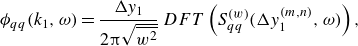(3.6) \begin{equation} \phi _{qq}(k_1,\omega ) = \frac {\Delta y_1}{2\unicode{x03C0} \sqrt {\overline {w^2}}}\, DFT\left (S_{qq}^{(w)}(\Delta y_1^{(m,n)},\omega )\right ), \end{equation}

where $\phi _{qq}$ is the wavenumber–frequency spectrum estimate, $\overline {w^2}$ is the windowing energy factor, and $DFT$ is the discrete Fourier transform operator.

3.3. Spanwise-averaged wall pressure spectrum estimate

Equation (3.6) provides the streamwise wavenumber–frequency spectrum that would be inferred from the array $\phi _{qq}$ , given the actual spectrum $\phi _{pp}$ . We can estimate the accuracy of the array by using a model for $\phi _{pp}$ and then comparing $\phi _{qq}$ with the original model spectrum spanwise averaged over the array width. Consider a streamwise line of points at a given spanwise location; the Fourier transform of the pressure measured by these points can be represented by $p(k_1,x_3,\omega )$ . For a sensor with a finite spanwise extent, the Fourier transform of the pressure averaged over this extent is expressed as

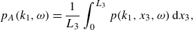(3.7) \begin{equation} p_A (k_1,\omega )=\frac {1}{L_3} \int _0^{L_3}p(k_1,x_3,\omega )\,{\textrm d}x_3, \end{equation}

where $L_3$ is the spanwise length of the sensor. We use this to obtain the wavenumber–frequency spectrum

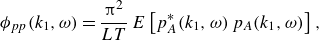(3.8) \begin{equation} \phi _{pp} (k_1,\omega )=\frac {\unicode{x03C0} ^2}{LT}\, E\left[p_A^* (k_1,\omega )\, p_A (k_1,\omega )\right], \end{equation}

where $L$ and $T$ are the half-ranges of the Fourier transforms for $k_1$ and $\omega$ . Substituting for $p_A$ ,

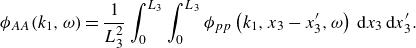(3.9) \begin{equation} \phi _{AA} (k_1,\omega )=\frac {1}{L_3^2} \int _0^{L_3}\int _0^{L_3}\phi _{pp} \left(k_1,x_3-x_3',\omega \right)\, {\textrm d}x_3\, {\textrm d}x_3'. \end{equation}

This can be evaluated numerically by assuming a discrete number of subdivisions of the spanwise length as $N\,\Delta x_3=L_3$ . We rewrite the above equation in its discretised form as

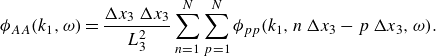(3.10) \begin{equation} \phi _{AA} (k_1,\omega )=\frac {\Delta x_3\, \Delta x_3}{L_3^2} \sum _{n=1}^{N}\sum _{p=1}^{N}\phi _{pp} (k_1,n\,\Delta x_3-p\,\Delta x_3,\omega ). \end{equation}

This can be reorganised as

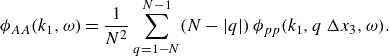(3.11) \begin{equation} \phi _{AA} (k_1,\omega )=\frac {1}{N^2} \sum _{q=1-N}^{N-1}(N-|q|)\,\phi _{pp} (k_1,q\,\Delta x_3,\omega ). \end{equation}

This formulation requires a choice of the $\phi _{pp}$ spectrum, $N$ and $\Delta x_3$ based on the sensor dimensions. We chose to use the modified Corcos model of $\S$ 2.3 to perform the initial error calculations used in array design, since its independent form for streamwise and spanwise scales makes it mathematically convenient, and its low sub-convective pressure levels (figure 3) make it a conservative choice for error estimation. The modified Corcos spectrum can be integrated over spanwise wavenumber as

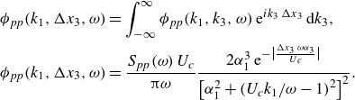(3.12) \begin{align} \phi _{pp} (k_1,\Delta x_3,\omega ) &= \int _{-\infty }^{\infty } \phi _{pp} (k_1,k_3,\omega )\, \textrm{e}^{ik_3\, \Delta x_3}\,{\textrm d}k_3, \nonumber\\ \phi _{pp} (k_1,\Delta x_3,\omega ) &= \frac {S_{pp} (\omega )\, U_c}{\unicode{x03C0} \omega } \frac {2\alpha _1^3\, \textrm{e}^{- \big| \frac{\Delta x_3\, \omega \alpha _3}{U_c} \big|}}{\left[\alpha _1^2+\left(U_c k_1/\omega -1\right)^2\right]^2}. \end{align}

As described in $\S$ 3.1, the sensor pore placement largely determines the sensitivity distribution, and this in turn will dictate the precise projection of the wavenumber–frequency spectrum as measured by a linear array of sensors given by (3.6). The predictions were studied against (3.11), which represented the ideal wavenumber–frequency spectrum targeted by an array of infinite sensors in the streamwise direction and finite spanwise extent.

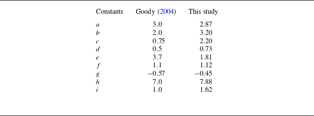
All Corcos-type models require a pointwise autospectrum model. The Goody model was chosen for this purpose; however, the empirical constants were adjusted to fit the wall pressure behaviour measured in the present flow. The choice was based on past studies (Fritsch et al. 2023) showing good agreement with measurements. The form of the Goody model used for this study is

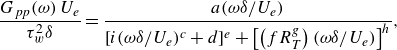(3.13) \begin{equation} \frac {G_{pp}(\omega )\,U_e}{\tau _w^2\delta } = \frac {a(\omega \delta /U_e)}{[i(\omega \delta /U_e)^c + d]^e + \left[\left(fR_T^g\right)(\omega \delta /U_e)\right]^h}, \end{equation}

where $R_T$ is the ratio of pressure time scales and is defined as $u_\tau \delta /\nu \sqrt {c_f/2}$ . The choices of constants for the model varied slightly from those of Goody (2004) based on a regression fit of measured data obtained by Damani et al. (2022), and are listed in table 1. The array tested was designed based on the modified Corcos model, hence the measured data were used to alter the constants for the modified Corcos model, namely the decorrelation coefficients. These were obtained by performing a nonlinear fit in a least squares sense, using the MATLAB function lsqcurvefit of the measured coherence to (2.10). The constant values ( $\alpha _1, \alpha _3$ ) obtained were 0.3275 and 0.77, respectively, as opposed to 0.1 and 0.77 recommended by Corcos (1967).

Table 1. List of constants in Goody model obtained from fitting measured data.

3.4. Array configuration and modelling results

The above approach applied to a series of candidate array designs, and using the boundary layer parameters of the present flow (table 2) quickly showed that arrays of streamwise-oriented sensors, such as suggested by Blake & Chase (1970) and investigated in our early work (Damani et al. 2022), can be subject to large errors due to aliasing, and even slight misalignment between the flow and the sensor axis. A variety of other configurations were considered before finalising the sensor array design; see § 5.3 of Damani (2025). A key finding of the mathematical model revealed that an array of spanwise-oriented sensors placed closely together along the flow direction was ideal for sub-convective pressure measurements.

Table 2. Boundary layer statistics for $Re_{c} = cU_\infty /\nu = 2 \times 10^{6}$ at $x_1= 2.64$ m.

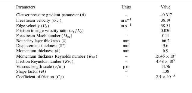
Figure 6 represents the final design. The array comprised 80 sensors covering length 440 mm, with 5.5 mm spacing between the sensors. Modelling results also showed better performance for continuous pore distributions along the flow direction, i.e. no discontinuity between sensor boundaries. This shows closer sensor spacing that reduces aliasing at lower wavenumbers by pushing the Nyquist limit to higher wavenumbers while still averaging a significant fraction of the convective energy by preserving the large area of the sensor. Unlike the array studied by Damani et al. (2022), which aimed to minimise aliasing and contamination from convective pressure fluctuations in the sub-convective region by using long sensors in the flow direction, this design acknowledges that while aliasing cannot be eliminated, it can be pushed to higher wavenumbers, making low wavenumbers free from aliasing. The linear arrangement also allowed multiple independent measurements of two-point correlations at separations smaller than the array length, which proved to be crucial in resolving the sub-convective pressure fluctuations.

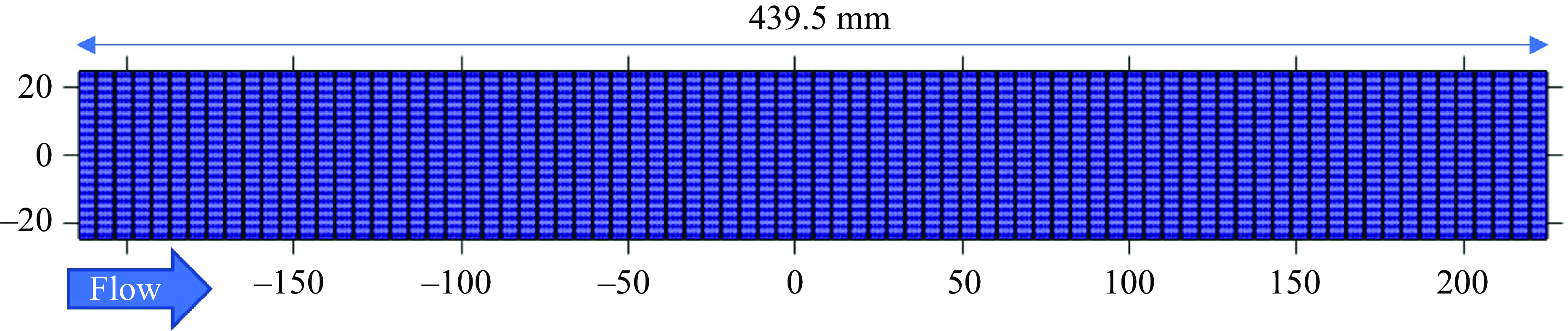
Figure 6. Full array layout showcasing 80 linearly arranged spanwise elongated sensors.

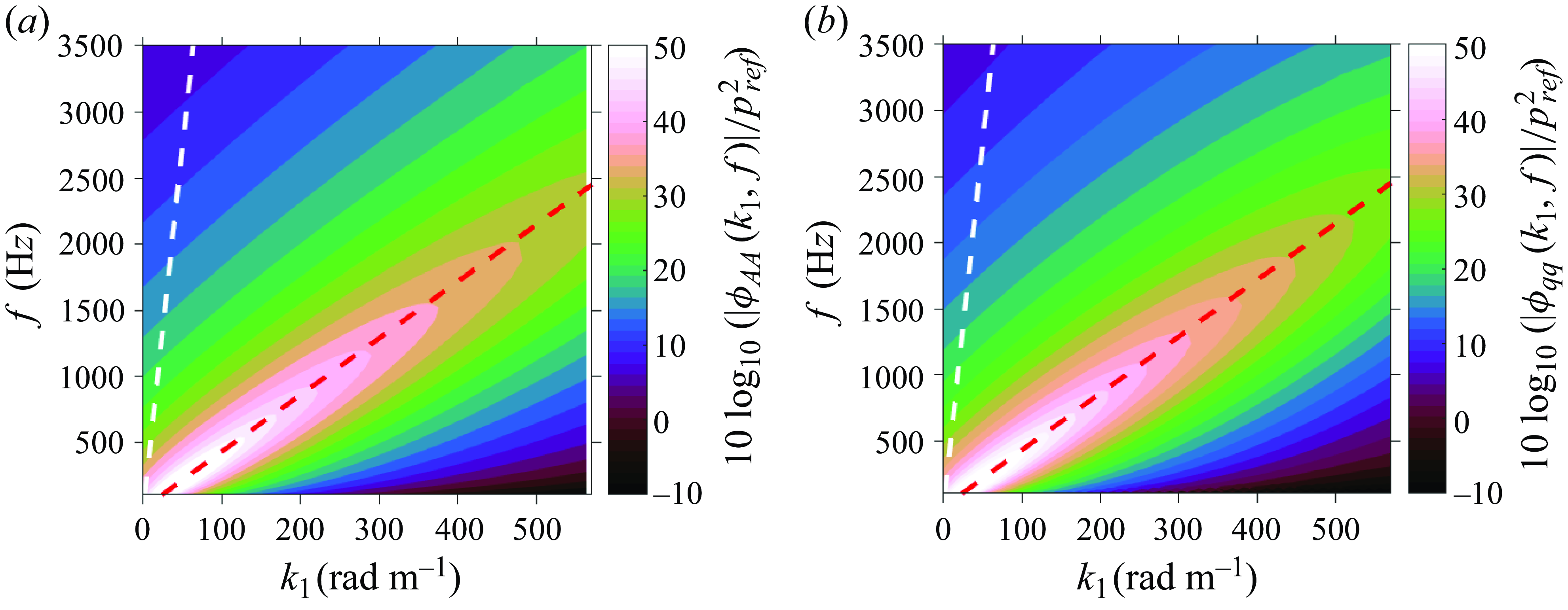
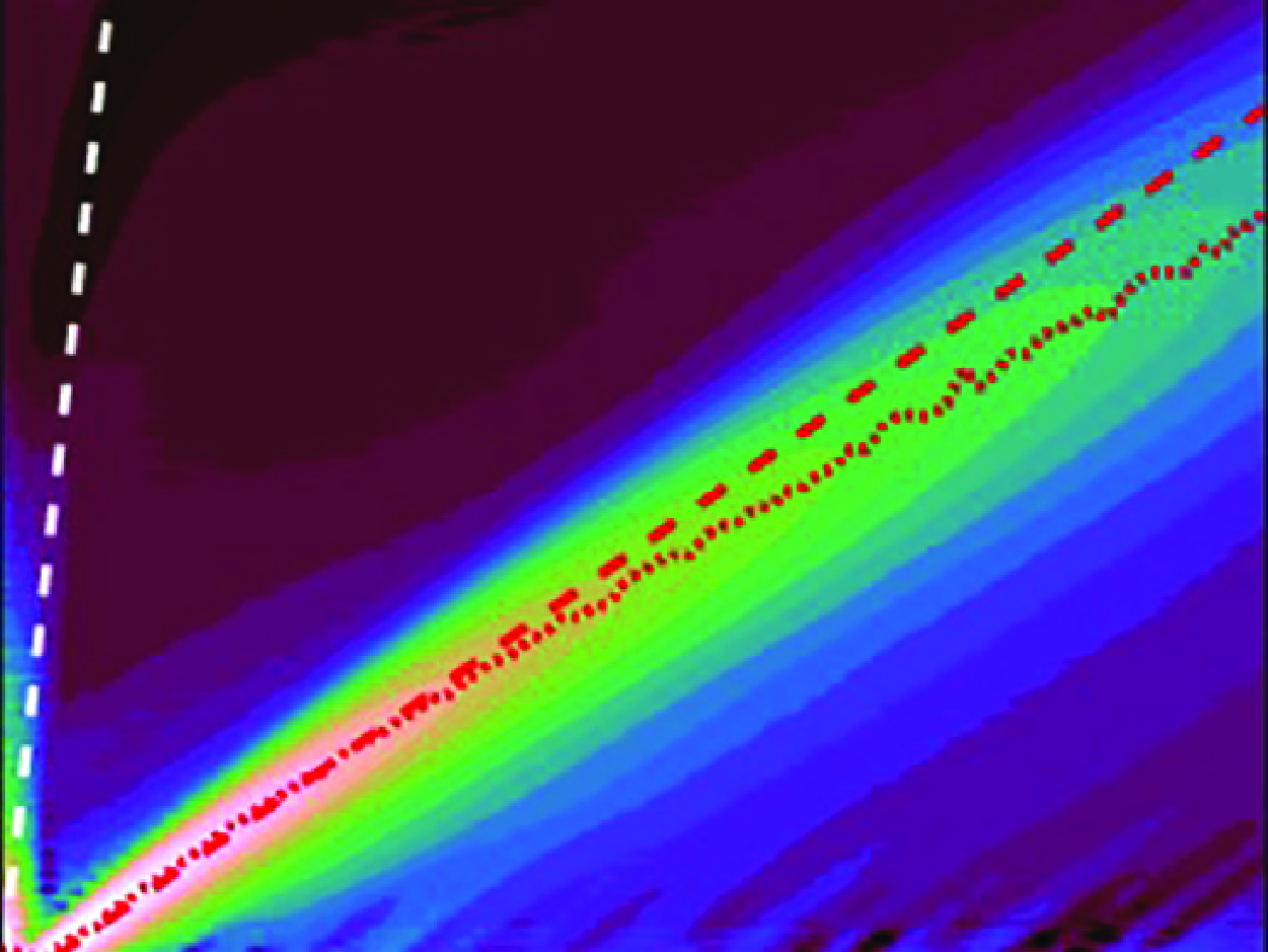
Figure 7. (a) Wavenumber–frequency spectrum averaged over a 50 mm span of the array. (b) Wavenumber–frequency spectrum estimate for an 80-sensor linear array. The red dashed line represents the convective line ( $U_c=0.7U_e$ ), and the white dashed line shows the sound line.

Figure 7(a) shows the modified Corcos wavenumber–frequency spectrum averaged over the 50 mm span of the array. This result serves as the reference for comparing the linear 80-sensor array performance. Figure 7(b) shows the wavenumber–frequency spectrum that would be measured by the array for uniform sensor sensitivity as modelled using the approach described in $\S$ 3.2. This plot is very similar to figure 7(a), indicating the capability of the 80-sensor array to regenerate the reference. The plots are cut off at 3500 Hz due to the sensors’ resonance frequency limit, which is based on the first cross-mode of the acoustic cavity. The differences are highlighted in figure 8(a), which plots the error between the predicted wavenumber–frequency spectrum and the spanwise-averaged spectrum evaluated using the modified Corcos model. Notice that the error in the low-wavenumber and low-frequency (sub-convective) domain is near 0 dB, showing that this pore distribution is an ideal candidate to manufacture the array. This also reflects on the performance of the array, showing that the levels in the sub-convective domain would be free of aliasing.

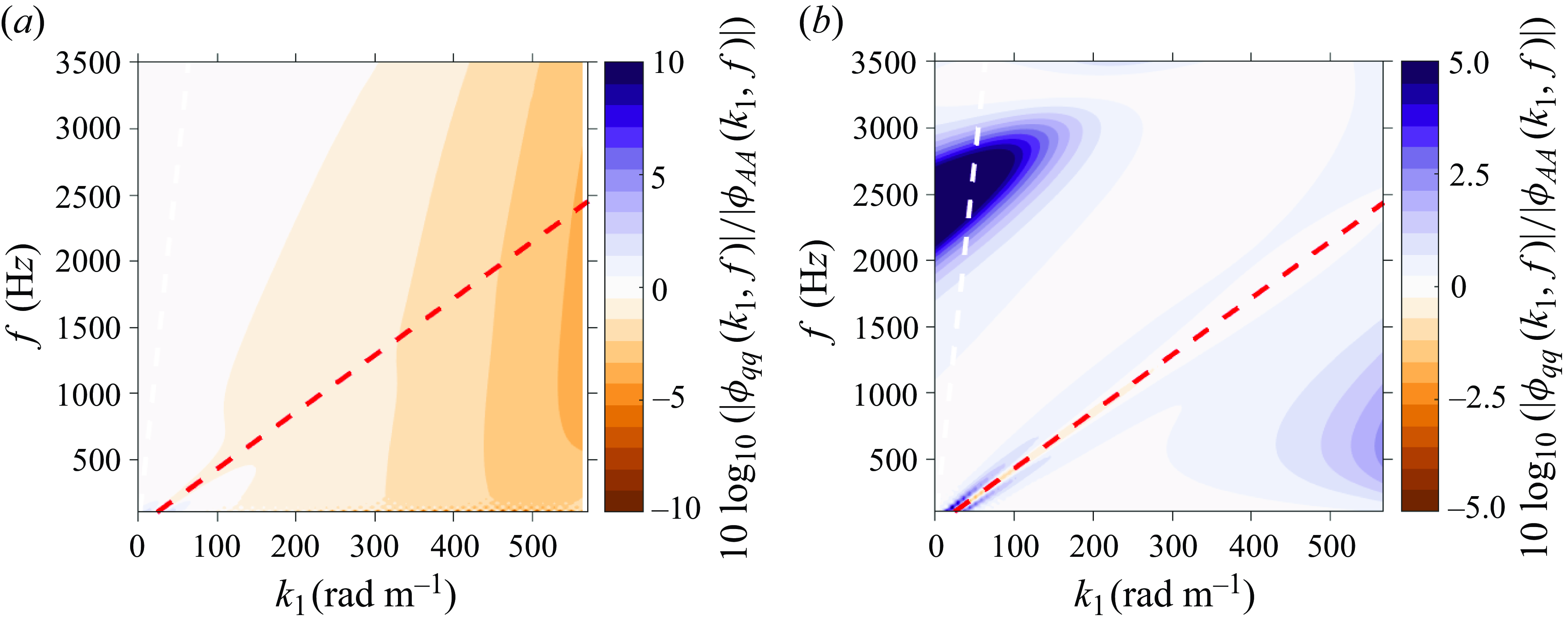
Figure 8. Error with respect to spanwise-averaged wavenumber–frequency spectrum: (a) modified Corcos model with uniform sensitivity; (b) Chase model with weighted sensitivity. The red dashed line represents the convective line ( $U_c=0.7U_e$ ), and the white dashed line shows the sound line.

The final error calculations for the array were performed after the wind tunnel experiment, at which point the Chase-like form of the actual pressure spectrum and the non-uniformity of the actual sensor sensitivity (figure 5) were known. The error estimates performed assuming a Chase spectrum and using the true non-uniform sensitivity are shown in figure 8(b). The results reveal aliasing artefacts at low wavenumbers and frequencies above 2000 Hz due to the biased sensitivity. Despite this, the error remains minimal in the sub-convective domain, indicating that the measurements are reliable in the region of interest, and that the specific model choice does not significantly affect the accuracy of the predictions in this regime.

4. Experimental methodology

4.1. Experimental set-up and boundary layer flow conditions

Measurements were carried out using the boundary layer grown on the port-side test wall of the Virginia Tech Stability Wind Tunnel. A top-down schematic of the experimental set-up is presented in figure 9. The port wall comprised a grid of modular panels (represented by the vertical black markings on the port wall in the figure), which were replaced with different instrumentation depending on the measurement. The turbulent boundary layer was initiated using a trip strip in the contraction chamber of the facility, resulting in a fully developed boundary layer at the inlet (marked as the origin in orange) of the test section. The inlet was the reference point for length measurements along the test section. The test section included a NACA 0012 aerofoil with the quarter chord ( $c=0.914$ m) located 3.45 m from the origin, spanning the full height of the test section. This imposed varying pressure gradients on the wall; however, this study focuses on a single pressure gradient condition corresponding to zero angle of attack, as shown in figure 9. The pressure variation along the test section was measured using static pressure taps distributed on the wall in the flow direction. The boundary layer profile was measured at $x_1=2.64$ m using a Pitot-static boundary layer rake (BLR) comprising 30 ports arranged logarithmically away from the wall. This set-up was similar to that of Vishwanathan (2023) and Fritsch et al. (2023). Results from these studies will be compared to the data presented in this paper, as the flow conditions were very similar. The sub-convective pressure sensing array (marked in yellow) was placed with its first sensor located 2.47 m from the origin.

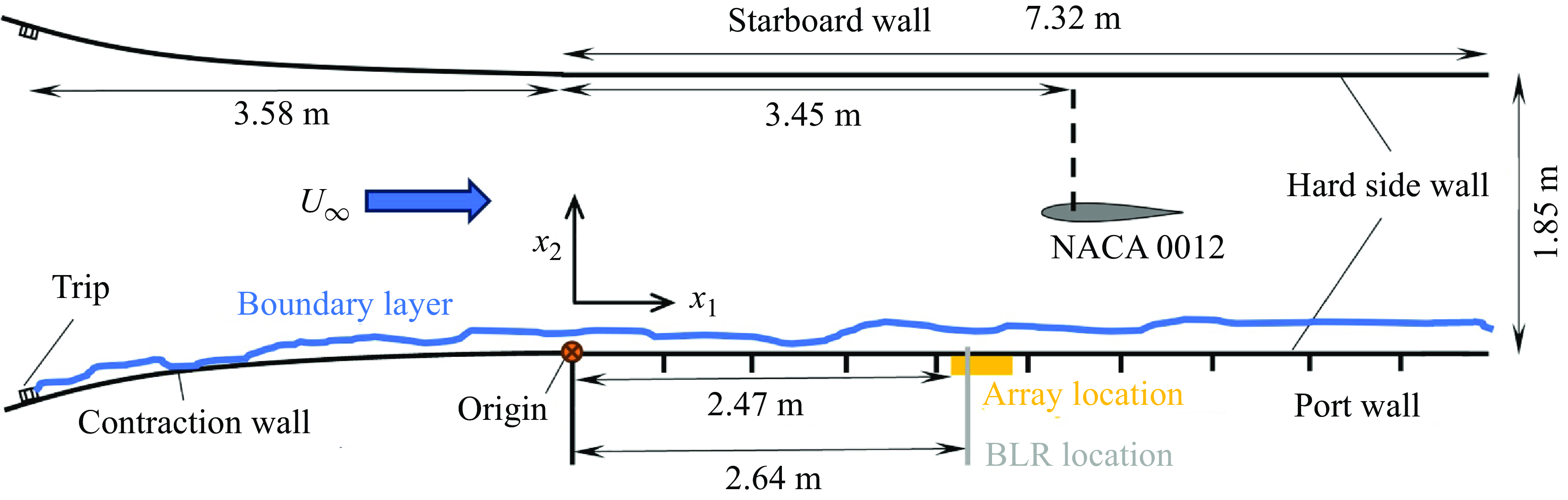
Figure 9. Top-down schematic of experimental test section in the Stability Wind Tunnel at Virginia Tech. The vertical black markings on the port wall represent individual panels that make up the test section. The yellow band represents the location of the sub-convective pressure sensing array.

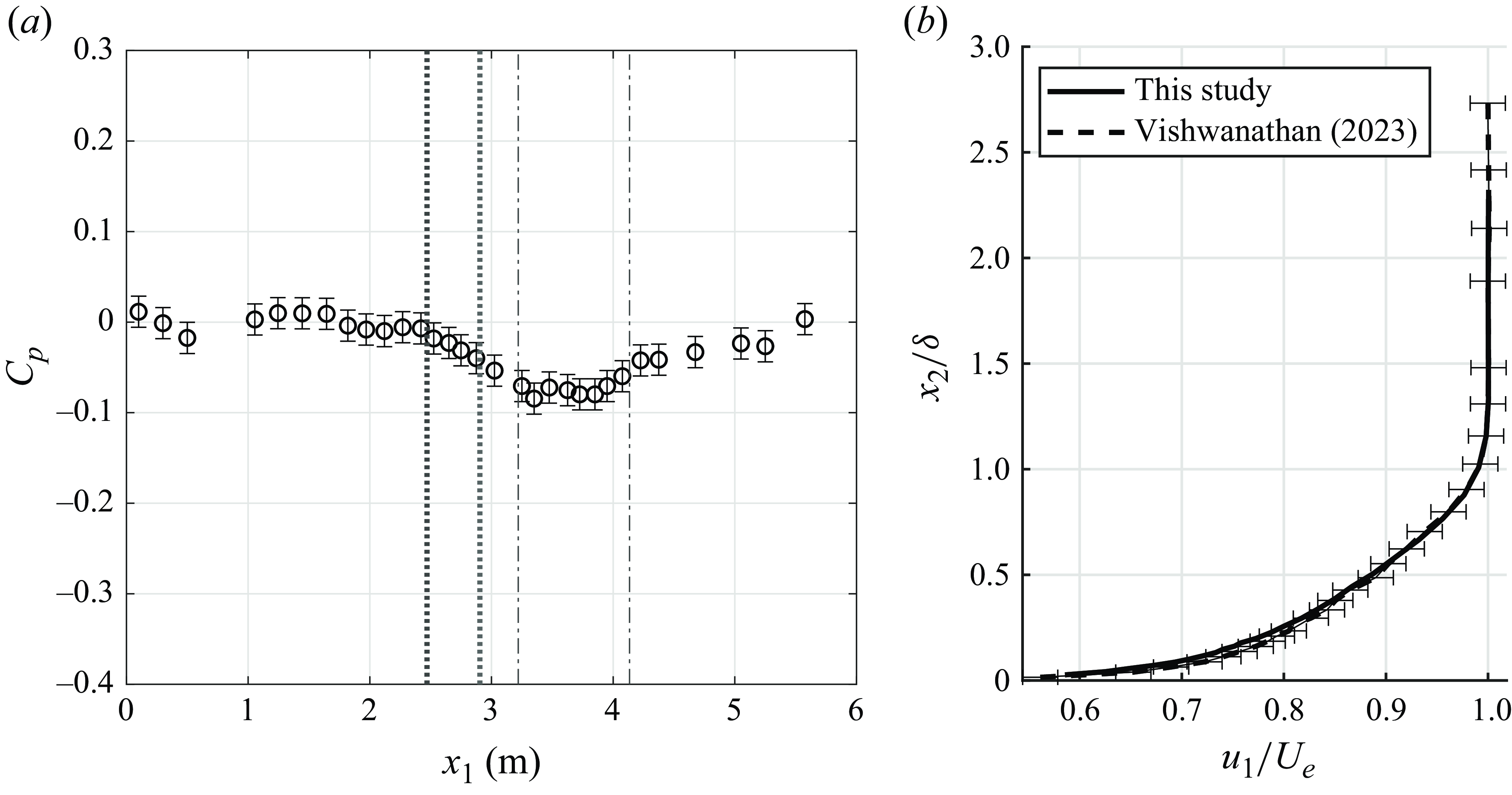
Figure 10. (a) Mean static pressure (error bars showing $1.96\sigma$ band for $C_p$ ) profile along test section with array marked with dashed black lines and aerofoil with dash-dotted lines. (b) Boundary layer profile compared against Vishwanathan (2023) (error bars showing $1.96\sigma$ band for $u_1/U_e$ ).

Figure 10(a) shows the mean static pressure distribution along the centreline of the port-side test wall, with the aerofoil leading edge shown at $x_1=3.22$ m spanning the region between the dash-dotted lines. It also marks the location and extent of the sub-convective array with dotted lines. Figure 10(b) compares the boundary layer profile acquired from this study with Vishwanathan (2023). It is important to note that the acquisition location of the rake in the present study was 0.1 m upstream of the study by Vishwanathan (2023), and the test section underwent a structural upgrade between the two datasets. Furthermore, the BLR instruments used in the two studies were different. Nonetheless, the profiles observe close agreement, with the differences lying within uncertainty. The boundary layer was spanwise uniform, as shown in Butt et al. (2023) using particle image velocimetry measurements, and Butt et al. (2024a ) using spanwise boundary layer traverse measurements. Relevant boundary layer parameters have been tabulated in table 2 for the flow condition considered in this study. The results from the modelling and the array design are described in detail in the following subsections.

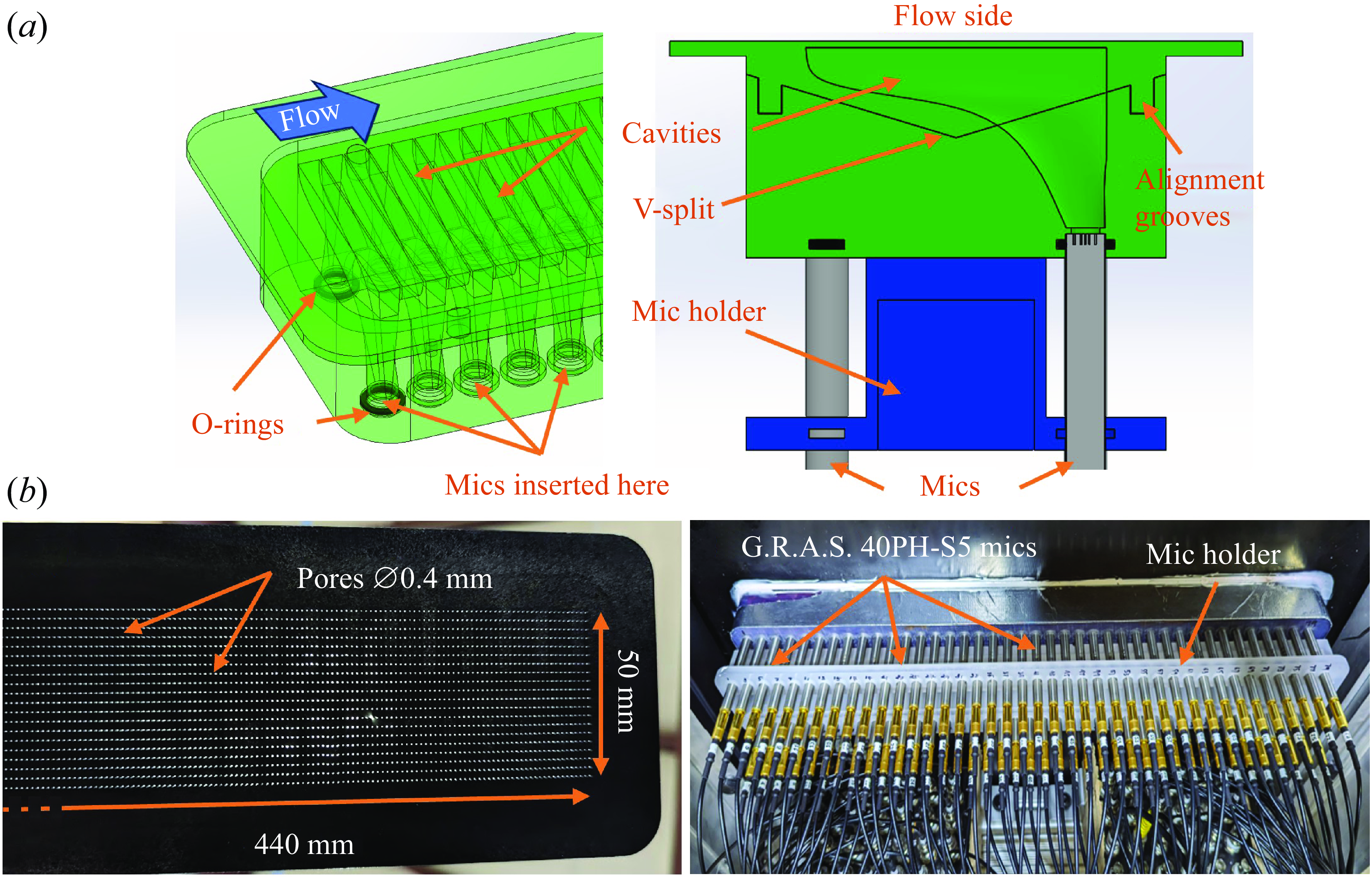
Figure 11. (a) A CAD model of the sensor array, highlighting its components and a cross-sectional view of a single cavity (pores omitted for clarity). (b) Photographic images of the fabricated array, showing the smooth top surface with pores, and the back side housing the microphones.

4.2. Production array and calibration

Figure 11(a) shows a computer-aided design (CAD) view of the array (green), microphone holder (blue), microphones (grey) and O-rings (black) to ensure a seal of individual sensors. The array was 3-D printed from Accura 60 (SLA) in two parts: an upper part including the flow surface and the upper portions of the sub-resonant cavities, and a lower part including the remainder of the cavities and the microphone supports. The two parts were joined along the 146 $^\circ$ V-shaped channel shown in the cross-sectional view of figure 11(a) using grease. Each sensor was pressure-checked to ensure a seal. The pores were drilled using a CNC machine after joining the parts. G.R.A.S. 40PH-S5 1/4” microphones were used, each with frequency range 10–20 kHz (flat frequency response within $\pm 1$ dB) and dynamic range 32 dB(A) to 135 dB. The sensors were linearly arranged with 5.5 mm spacing (Nyquist wavenumber 571.2 rad m $^{-1}$ ), with adjacent sensors mirrored along the streamwise axis. The maximum centre-to-centre separation between sensors was 434.5 mm, corresponding to wavenumber resolution 7.23 rad m $^{-1}$ .

Data were sampled using an 18-bit, 128-channel simultaneous sampling system at 25 600 Hz over 320 s for each flow condition. This long sampling duration was chosen to improve the signal-to-noise ratio for the low-magnitude sub-convective pressure fluctuations, which agrees with observations made by Abtahi et al. (2024a ). This duration was also limited by the volume of data stored in the data acquisition memory. The frequency spectrum was analysed by dividing the time signal into 5000 records, each consisting of 4096 samples. Each record represented 0.16 s of data, and the spectrum was calculated using the pwelch method with 50 % overlap and a Hanning window.

The array of multi-pore Helmholtz resonating sensors required a bulk dynamic calibration to account for cavity dynamics and any phase discrepancies between the microphones. This was obtained using a two-step calibration procedure involving a surface pressure measurement and an array measurement. An omnidirectional source (HBK Type 4292-L) placed in the far field was used. The surface pressure measurement used HBK Type 4144 and 4145 1 inch microphones. The individual sensors on the array were calibrated simultaneously, utilising a time delay factor based on source path length relations. Dividing out the spectral response from the two measurements yielded individual sensor response functions accounting for magnitude and phase corrections. Their form was similar to observations made by Damani et al. (2025) on cavity sensors. Each sensor experienced a shift in response due to impedance changes from grazing flow effects (Fritsch et al. 2021; Li & Choy 2024). The shift in resonant frequency was found to be within 300 Hz, and the magnitude observed a variation within 2 dB relative to 1 V Pa⁻¹. The modelling approach described in $\S$ 3 was utilised to back out the shift in response functions. Specifically, (3.5) was evaluated for the distribution of 80 pores on the sensor, and the Goody model (3.13) was used as the autospectral density function. A more precise calibration technique would employ a direct relation between the shear stress and its effects on the resonance of an arbitrarily shaped cavity; however, this was not available.

4.3. Additional measurements

Comparative measurements were also taken using six linearly spaced HBK Type 4144 and 4145 1 inch microphones (23.7 mm diaphragm size), this being the same as the microphone array used by Farabee & Geib (1991). This array is referred to as the F&G array hereafter, and a green colour will be used for its results. When used, it was installed at the same location as the sub-convective pressure sensing array with its first microphone at $x_1=2.51$ m, equivalent to the position of the seventh sensor on the sub-convective array. Note that a single microphone on the F&G array covered a streamwise extent just short of four sensors of the sub-convective array. Figure 12 shows the view of the array with the microphone diaphragms that were exposed to the flow. Data were acquired at sampling rate 65 536 Hz for 256 s using an HBK Type 3050 Multipurpose 6-channel DAQ module. The spectrum analysis was conducted using record size 8192 samples, 50 % overlap, and a Hanning window. It is important to highlight the differences between the measurements by the array and the F&G array. This mainly concerns their spanwise extent (sensor 50 mm, and F&G microphone 23.7 mm), which creates a difference in averaging. Comparing the results when normalised on their autospectrum helps to account for this averaging difference, as will be discussed in $\S$ 5.1.

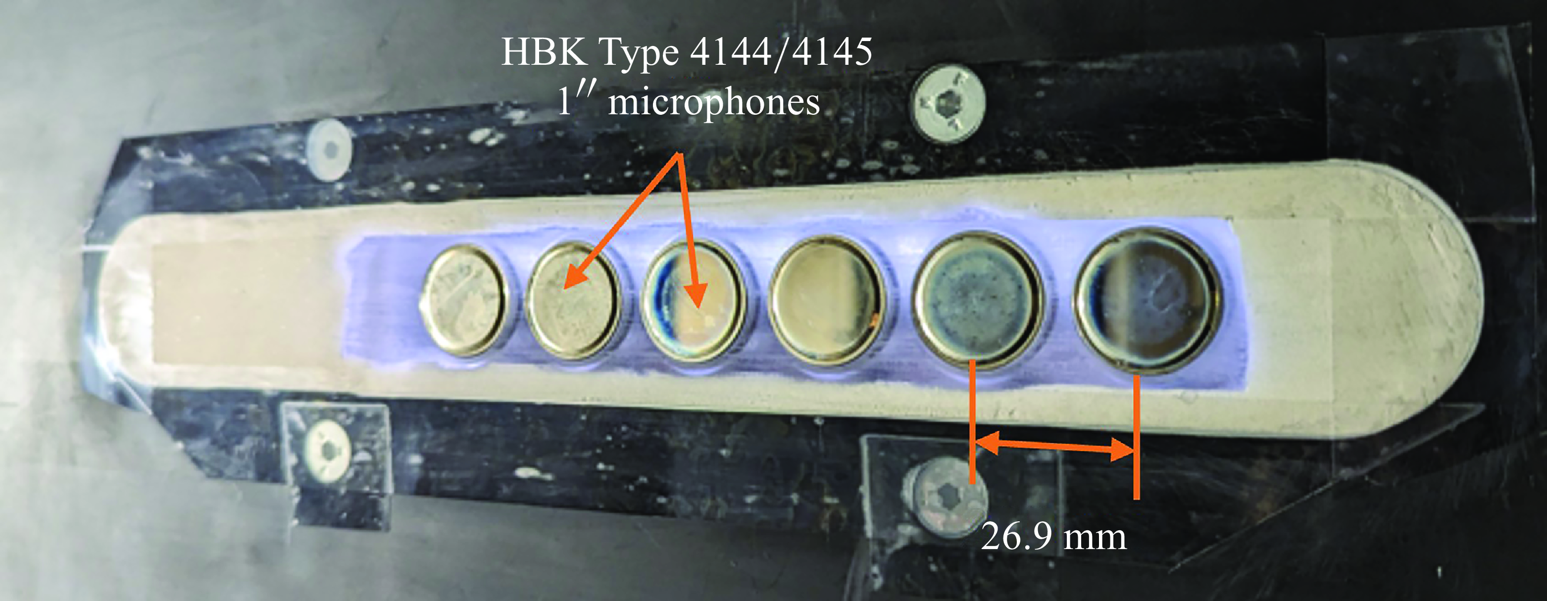
Figure 12. An array of six 1 inch HBK type 4144/4145 microphones used by Farabee & Geib (1991).

Only the first four microphones were usable in the present study due to inconsistencies observed in the last two. Farabee & Geib (1991) analysed data using sum and difference modes to isolate wall pressure levels in the sub-convective and acoustic regions. The sum mode, which phases signals in unison, filters out all but wavelengths corresponding to $\lambda = L/m$ , where $L$ is the microphone spacing, and $m$ is an integer. The difference mode, applying an alternating phase, isolates wavelengths at ( $\lambda = 2L/(2m+1)$ ), corresponding to wavenumbers $k_1L = (2m+1)\unicode{x03C0}$ and $k_1L = 2m\unicode{x03C0}$ for difference and sum modes, respectively. Using this methodology, a working wavenumber $k_1\delta ^*=1.12$ and frequencies 2.5 kHz ( $\omega \delta ^*/U_{\infty }=3.9$ ) for the sub-convective region, and 6 kHz ( $\omega \delta ^*/U_{\infty }=9.4$ ) for the acoustic region, were identified. A more refined wavenumber–frequency spectrum can be obtained through cross-spectral density analysis and spatial Fourier transformation. However, the small number of microphones, large sensing areas and wide spacing limit the wavenumber range and resolution. The Nyquist limit is 116.78 rad m⁻¹, with resolution 38.9 rad m⁻¹. Measurements were conducted at a lower Reynolds number ( $\delta =69.7$ mm, $\delta ^*=10.4$ mm, $\theta =7.4$ mm, $Re_{\tau }=3320$ ) to prevent damage to exposed microphone diaphragms. The measurements were scaled to the high Reynolds number data shown in this study based on normalisations.

5. Results and discussion

This section presents measurements from the wall pressure sensing array for the case described in table 2 in the form of cross-spectrum and wavenumber–frequency spectrum. First, a note on the flow statistics convergence is presented to establish noise floor levels and limitations of the measurements, which is crucial for inferences. Each subsection details a description of the measured data and its comparison with model estimates that account for area averaging of the sensors. The wall pressure wavenumber–frequency models do not account for pressure gradient, but in the past have been used for comparison with both zero and non-zero pressure gradient flows (Goody 2004; Hwang, Bonness & Hambric 2009). Hence the choice of wall pressure models for this study is justifiable. Also, the overall aim was to perform a rudimentary comparison to highlight the differences in the sub-convective domain. Measurements from the F&G array are also compared at overlapping wavenumbers and frequencies.

5.1. Flow convergence and homogeneity

Multiple datasets were combined to understand the statistics of the wall pressure fluctuations. Flow convergence is studied using the average coherence between all possible sensor pairs on the array. As an example, the averaged $12$ th-octave binned coherence corresponding to $\Delta x_1/\delta ^*=15.3$ is shown in figure 13. The average represents the mean of 51 possible sensor pair combinations corresponding to $\Delta x_1/\delta ^*=15.3$ . The plots present the coherence as a function of frequency for different sampling durations. The frequency has been normalised on the time scale $\delta ^*/U_\infty$ , and the legend indicates the durations as multiples of the same time scale. The curves represent time scales from $7 \times 10^5$ to $10^7$ times $\delta ^*/U_\infty$ , corresponding to 4000–60 000 spectral averages. The lowest coherence levels drop to $-35$ dB for the shortest average time, to approximately $-45$ dB for the longest. The continuing drop in levels with averaging time implies that the results are still converging, and that the measurement system’s noise floor has not been reached. We speculate that this very slow convergence is due to the meandering nature of superstructures (Hutchins & Marusic 2007). This convergence limitation is also observed in the flow visualisation results discussed in Butt et al. (2023), and is per the observations of Abtahi et al. (2024a ).

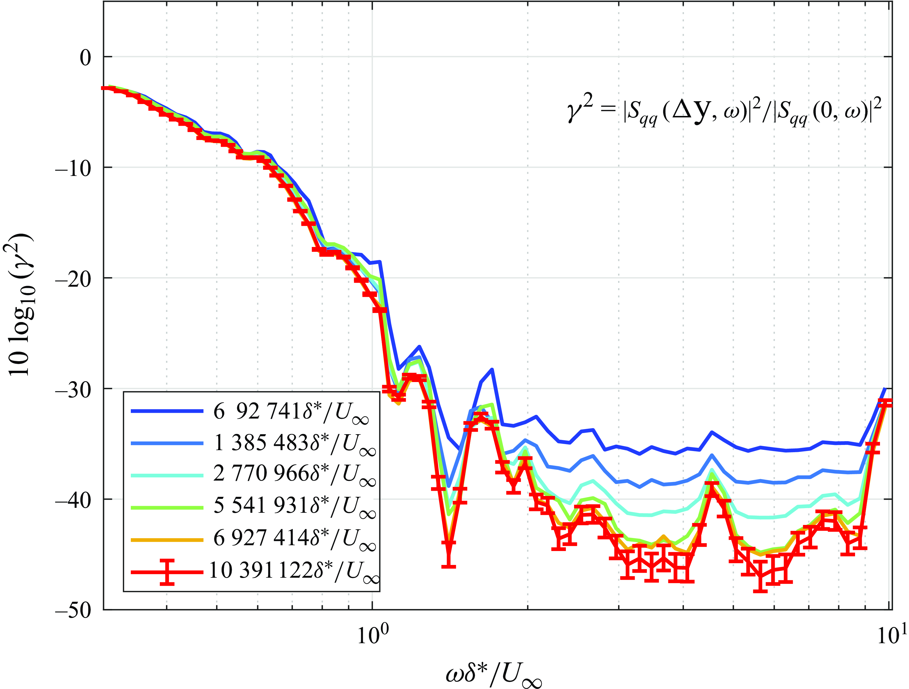
Figure 13. Average binned coherence between sensors ( $\Delta x_1/\delta ^* = 15.3$ ) for different sampling durations, showing convergence of statistics. Uncertainty estimates are shown for the longest temporal duration case.

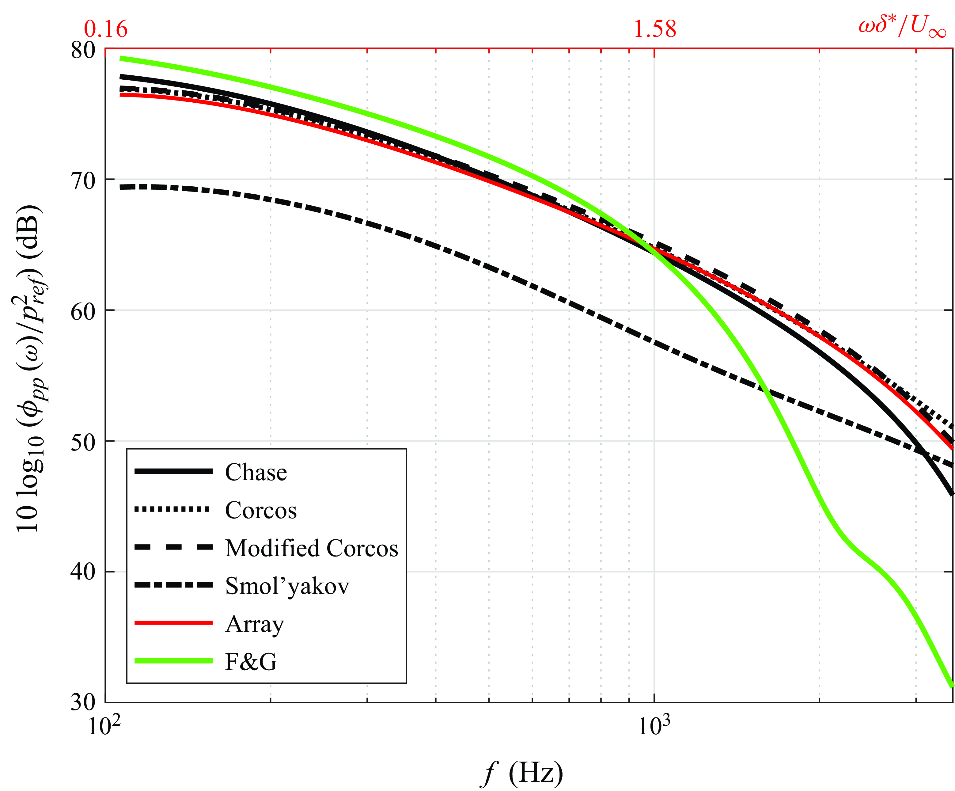
Figure 14. Autospectra comparison between area-averaged model predictions, measured data and pointwise estimates. The uncertainty in the array measurement is $\pm 1$ dB.

Figure 14 compares the measured pressure autospectra for the sub-resonant array with estimates from various wall pressure models of $\S$ 2, scaled using the boundary layer parameters of table 2, and averaged over the 50 mm $\times$ 5 mm sensor area. Also included is the autospectrum measured by the F&G array of microphones, which represents averaging over the 23.6 mm diameter of its sensors. The plot levels are presented in sound pressure level (dB/Hz relative to 20 $\unicode{x03BC}$ Pa). The Corcos, Smol’yakov and modified Corcos models use the Goody pointwise model of $\S$ 3.2 to evaluate the area-averaged form. Results from the F&G array estimated by a model are also shown in solid green. The agreement between the sub-resonant array measurement and all models except the Smol’yakov is excellent at low frequencies, with minor discrepancies emerging at higher frequencies as area-averaging effects become more significant. This shows that the flow-based calibrations discussed in $\S$ 4.2 are independent of the model chosen, except the Smol’yakov model. The Smol’yakov model significantly underestimates the levels because of the much larger (and apparently unrealistic) effect of sensor area averaging on its result. The F&G microphones show a pressure spectrum with a steeper roll-off at 1000 Hz, attributed to the larger surface area of the microphones and their Bessel-function-like area sensitivity.

Uncertainty estimates presented with the cross-spectra and wavenumber–frequency spectra in the following subsections were obtained by classifying sources as bias or random uncertainty. Sources of bias uncertainty include variations in flow speed inside the test section throughout the sampling period, the bias due to boundary layer growth over the array, and the bias due to sensor calibrations. The uncertainty in the flow speed was found to be 0.11 m s $^{-1}$ (0.3 % error). This corresponds to pressure uncertainty 0.025 dB, which was accounted for in cross-spectrum and wavenumber–frequency spectrum uncertainty calculations. The boundary layer growth and favourable pressure gradient experienced at the measurement location make it challenging to separate the uncertainties. The autospectrum had uncertainty 1 dB, considering the sensor-to-sensor variation and flow inhomogeneity across the array’s length. Random uncertainty was evaluated using relations given by Bendat & Piersol (2010), mainly for autospectrum, cross-spectrum and phase. An uncertainty propagation analysis was performed to find the random uncertainty in the wavenumber–frequency spectrum. Random uncertainty is also observed in individual sensor responses, which show a variation of 0.6 dB relative to 20 $\unicode{x03BC}$ Pa. This shows consistency with the sensor–sensor variation, and can be used in the total uncertainty estimate.

5.2. Cross-spectrum

Figure 15 shows the averaged cross-spectrum magnitude and the unwrapped phase. The averaged cross-spectrum was evaluated by considering all possible combinations of sensor pairs as a function of streamwise separation, and obtaining the average. Both contours are shown as a function of frequency in hertz, and streamwise distance in metres. The colour scale on the cross-spectrum plot (figure 15 a) represents the spectrum levels in dB relative to 20 $\unicode{x03BC}$ Pa. Non-dimensional axes have also been indicated in red, with the non-dimensional spectra levels (not shown) scaled as $S_{qq}U_\infty /\tau _w^2\delta ^*$ , i.e. a factor $1026.1p_{ref}^2=-63.8$ dB. Regions in high frequencies and separations are omitted (seen as white) due to a minimum coherence criterion ( $\gamma ^2_{min}=0.002$ ). An exponentially decaying form can be observed as a function of spatial separation at a fixed frequency. Considering a frequency slice at low frequencies (below 300 Hz), the variation in levels shows a periodic drop in levels (associated with the green colour) at specific separations. For instance, at $f=125$ Hz, one observes a drop in levels at $\Delta x_1=0.11$ and 0.33 m. As we will see later, this side-lobe-type behaviour is a result of the surprising compactness of the convective ridge in the wavenumber domain. The uncertainty in the magnitude of the cross-spectrum is approximately 3 dB in the region shown, and higher in the omitted high-frequency and larger-separation region. The magnitude plot shows faint vertical comb-like features in the streamwise direction at intervals of 0.011 m, particularly around 1 kHz and $\Delta x_1=0.05$ m. This artefact is an attribute of the non-uniform area sensitivity over the sensor, as discussed in $\S$ 3.1.

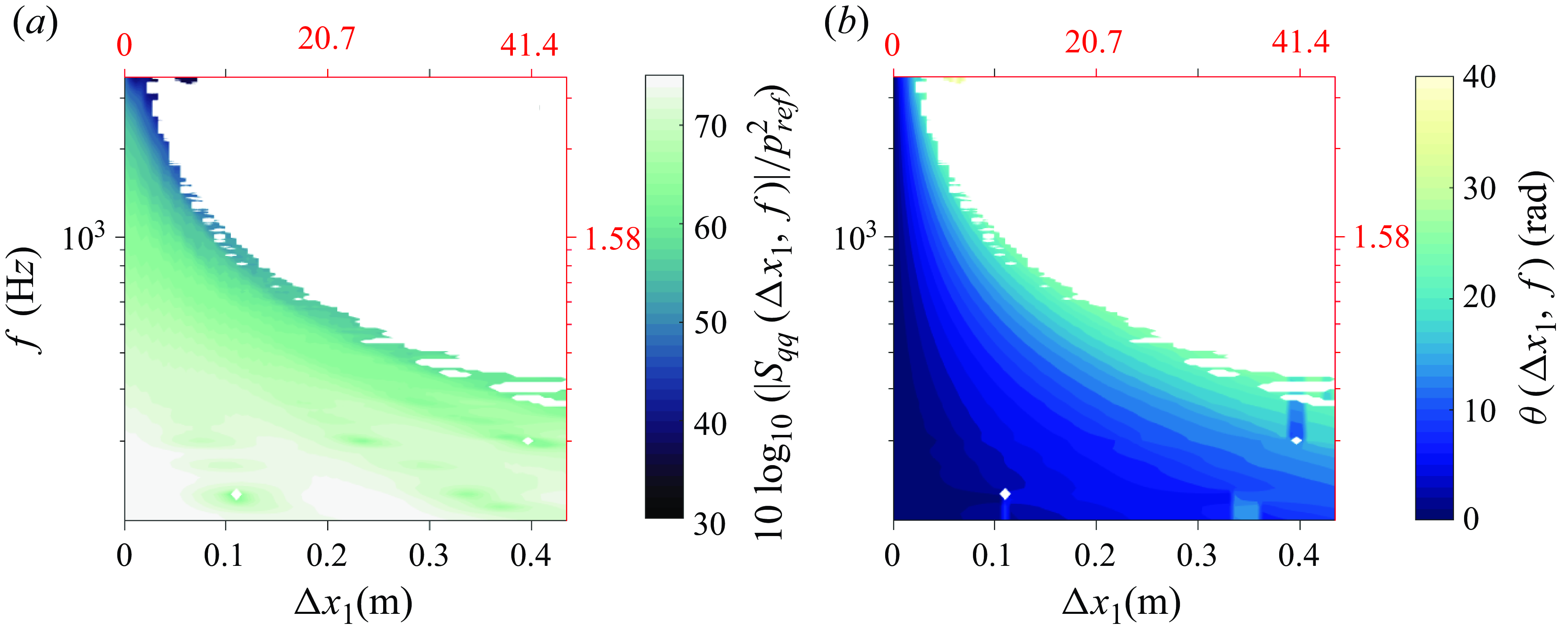
Figure 15. (a) Measured cross-spectrum magnitude and (b) unwrapped phase, as functions of frequency and streamwise separation. The red axes represent non-dimensional streamwise distance ( $\Delta x_1/\delta ^*$ ) and frequency ( $\omega \delta ^*/U_\infty$ ).

The phase (figure 15 b) represents an interesting behaviour comprising a main lobe where the phase increases almost linearly with both frequency and streamwise separation. Showing the phase contour is important to identify the plausible relationship between sub-convective pressure fluctuations and the coherent motions in the boundary layer. Considering the physical flow, the coherent motions move at a bulk speed in the range $60{-}80\,\%$ of the edge velocity. The pressure perturbations matching the convective motion are registered in the convective ridge. It has been established that the convective phase evolves nonlinearly with frequency (as modelled by Smol’yakov 2006), but the quantity of interest is the relation of phase to sub-convective wavenumbers. Considering a specific frequency, the phase relation for convective pressure fluctuations is known; however, the unwrapped phase shows deviations from this relation, representing the dispersion of pressure waves into wavenumbers not corresponding to convective motions. This yields much higher phase speeds of pressure waves, which may or may not correlate with anything physical in the fluid. This deviation can be sourced from various possibilities, including convective motions tracing the surface at angles, or the evolution of coherent motions in space and time. Further investigation is needed to clearly show the relation between sub-convective pressure fluctuations and coherent motions.

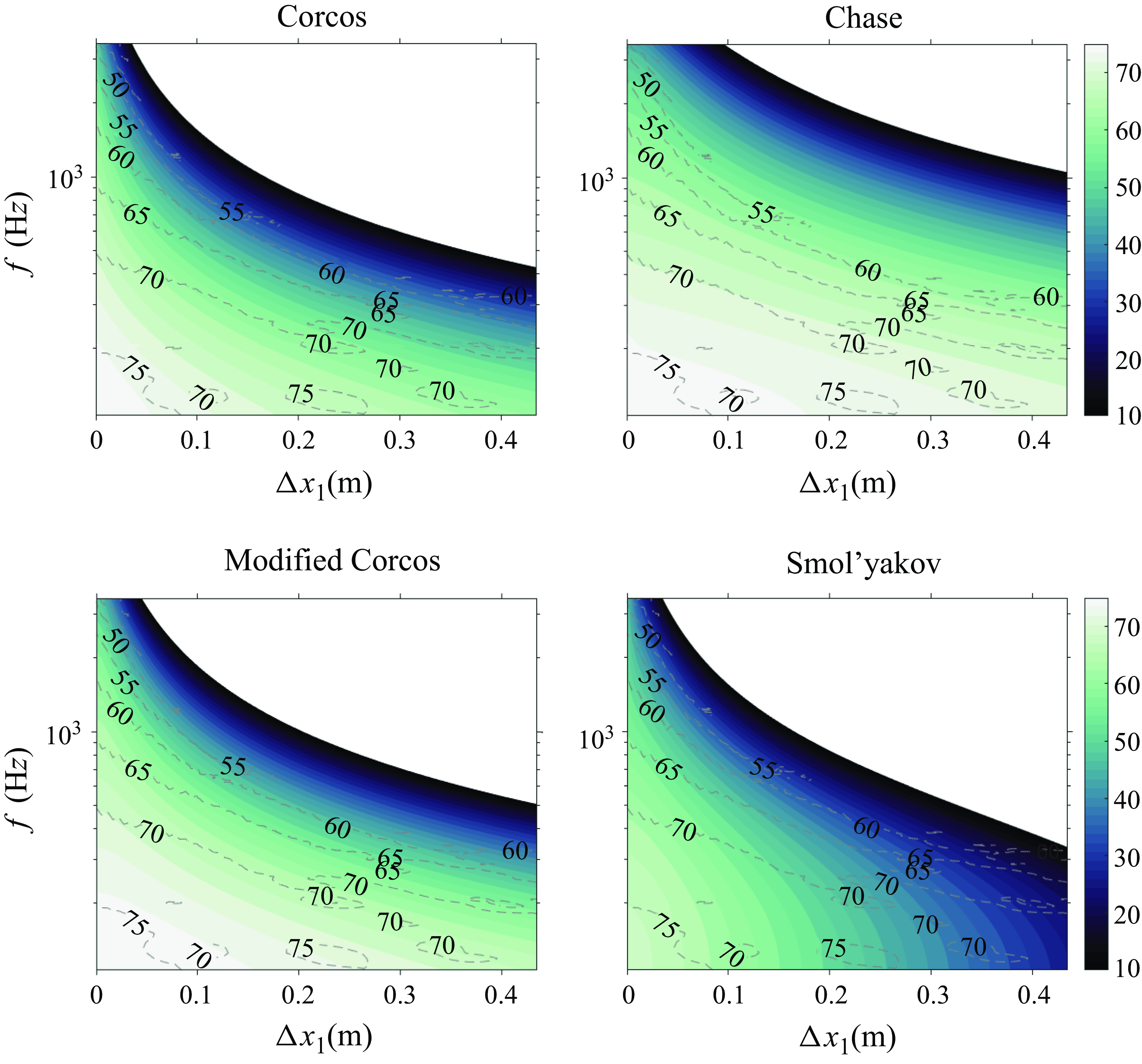
Figure 16. Cross-spectra estimates from various models for the array of sensors superimposed with the measured data as dashed contour lines.

Figure 16 compares the measured cross-spectral magnitude with the predictions made using the models of $\S$ 3. The colour scale depicts the magnitude of the cross-spectra estimates in dB rel. 20 $\unicode{x03BC}$ Pa. The non-dimensional axes are avoided here to prevent visual clutter; however, the same axes as figure 15 apply, along with the colour bar scaling. The model predictions are made using (3.5), accounting for the sensor averaging. They show exponentially decaying behaviour with respect to frequency and streamwise separation, similar to the measurements. The contour levels have been limited for convenience to compare with figure 15. This creates a white region at high frequencies, and separations representing omitted colour levels. Each contour also shows dashed contour lines from the measured data within colour limits 45 and 75 dB. The Corcos and modified Corcos models have very similar predictions except for a minor difference in their decay behaviour, with the Corcos model showing a sharper decay. The Chase estimate shows much slower decay, which agrees closely with the measured data identified by the hard-to-distinguish measured data (dashed lines) from the filled contours. The Chase model has a large spread in separation, while the Smol’yakov model seems to have the fastest decay as a function of separation. The behaviour at larger separations appears to be different for the Smol’yakov model compared to the others. It shows a truncated nature, while other models show a smoother decay. A comparison between the colour contours from the model predictions and the dashed contour lines from the measurements reveals differences in decay behaviour. Both the Corcos and Smol’yakov models predict faster decay with streamwise distance than observed in the measurements. In contrast, the Chase and modified Corcos models show better agreement with the experimental data, with the Chase model exhibiting the closest match.

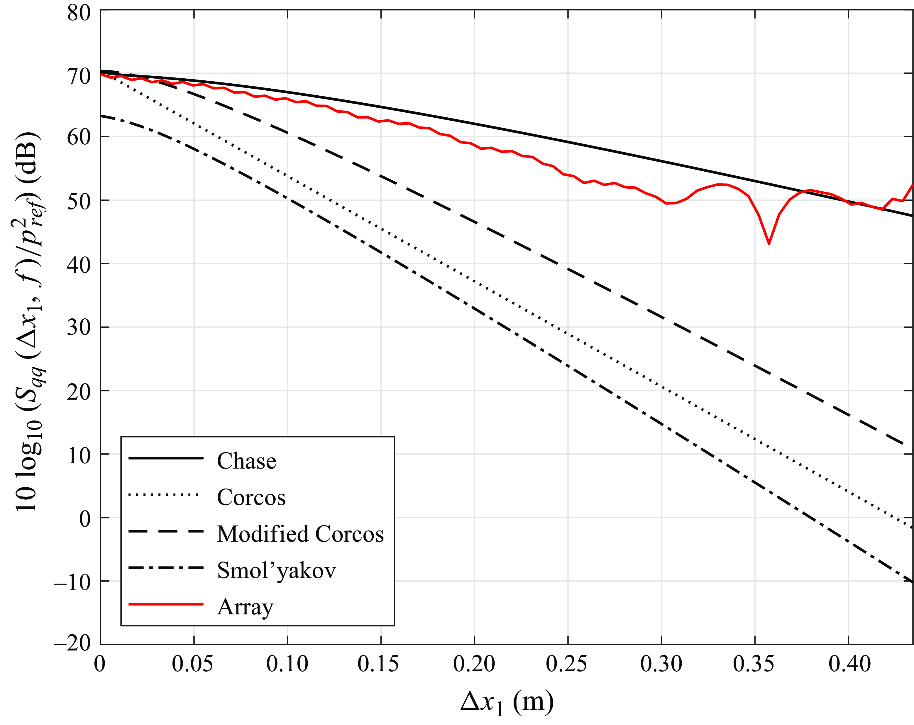
Figure 17. Comparison of cross-spectral magnitude at $f=510$ Hz ( $\omega \delta ^*/U_\infty = 0.8$ ).

An example slice of the cross-spectrum magnitude relative to 20 $\unicode{x03BC}$ Pa is shown in figure 17. This yields a direct comparison of levels and the behaviour as a function of streamwise separation at a fixed frequency ( $\omega \delta ^*/U_\infty =0.8,\ f=510$ Hz). It shows considerably better agreement with the Chase model than with any of the others. The behaviour at higher separations ( $0.3 \leqslant \Delta x_1 \leqslant 0.43$ ), including the sharp feature at $\Delta x_1=0.36$ , is in the region where the measurement coherence is only marginally significant, as seen in figure 15(a). It can be seen from this comparison that the other models – Corcos, modified Corcos and Smol’yakov – perform poorly in predicting the trend of the cross-spectrum decay. These overpredict the decay rate, giving rise to much steeper plots. The Smol’yakov model shows a discrepancy at $\Delta x_1=0$ due to the difference observed in the autospectrum in figure 14.

5.3. Wavenumber–frequency spectrum

Taking the Fourier transform of the cross-spectrum along the spatial separation direction yields the wavenumber–frequency spectrum. Figure 18 presents this spectrum, with wavenumber on the $x$ -axis and frequency on the $y$ -axis. Non-dimensional axes have also been indicated in red, with the non-dimensional spectra levels (not shown) scaled as $\phi _{qq}U_\infty /\tau _w^2\delta ^{*2}$ , i.e. a factor of $1.06 \times 10^5p_{ref}^2=-43.7$ dB. The figure highlights three distinct regions: supersonic (left of the white dashed line), sub-convective (between the dashed lines), and convective (around the red dashed line). The white dashed line marks the sound line, while the red dashed line represents the nominal convective line ( $\omega _c/k_c=0.7U_e$ ). The pressure spectrum peaks near the convective line, representing the fluctuations moving with the mean bulk motion of the fluid. The region inside the white dashed line represents sound waves grazing the surface. These can arise due to acoustics in the facility, and convective motions giving rise to near-field acoustics. The area between the lines is the focus of this study, which highlights a wavenumber-dependent behaviour at low frequencies, and a wavenumber-white behaviour at higher frequencies. There appears to be a strict boundary on the left-hand side of the convective ridge (in the sub-convective domain) beyond which a rapid reduction in levels is observed. Additionally, the convective ridge shows a decrease in slope with increasing wavenumber, indicating a frequency-dependent convective velocity. This is marked using the dotted red line, which tracks the peak of the spectral levels. The right-hand side of the convective ridge shows a larger spread, implying that the convective ridge is not symmetric. The diagonal features at low frequencies and high wavenumber in the super-convective regime indicate a lack of sufficient resolution in frequency. The uncertainties in the cross-spectrum were propagated in the wavenumber–frequency domain, yielding uncertainty bounds $\pm 1.5$ dB. This includes the bias uncertainty in the freestream velocity, inhomogeneity due to boundary layer growth, and random uncertainty due to sensor–sensor variation. The boundary layer growth was very small, with maximum variation 6 % in the boundary layer parameters between the most upstream and downstream points. This difference was modelled and propagated to the wavenumber–frequency spectrum. The errors were within $\pm 1.5$ dB, with the largest errors seen at the transition between the convective ridge and the sub-convective domain.

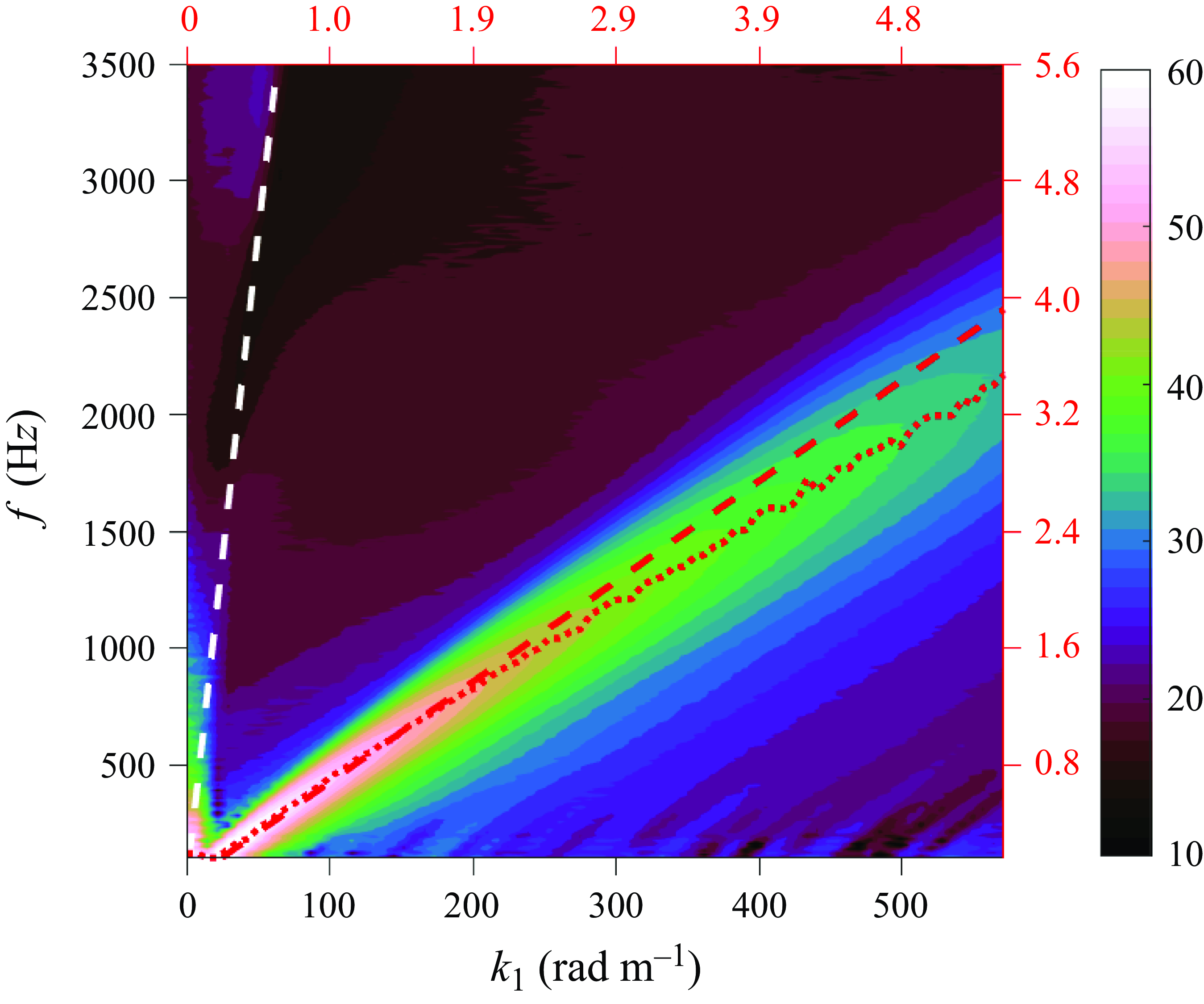
Figure 18. Measured wavenumber–frequency spectrum. The red axes represent non-dimensional streamwise wavenumber ( $k_1 \delta ^*$ ) and frequency ( $\omega \delta ^*/U_\infty$ ). The white dashed line is the sound line ( $k_1=\omega /c_0$ ), the red dashed line is the convective line assuming constant convective velocity ( $k_c=\omega /U_c$ ), and the red dotted line is the locus of the convective ridge peak.

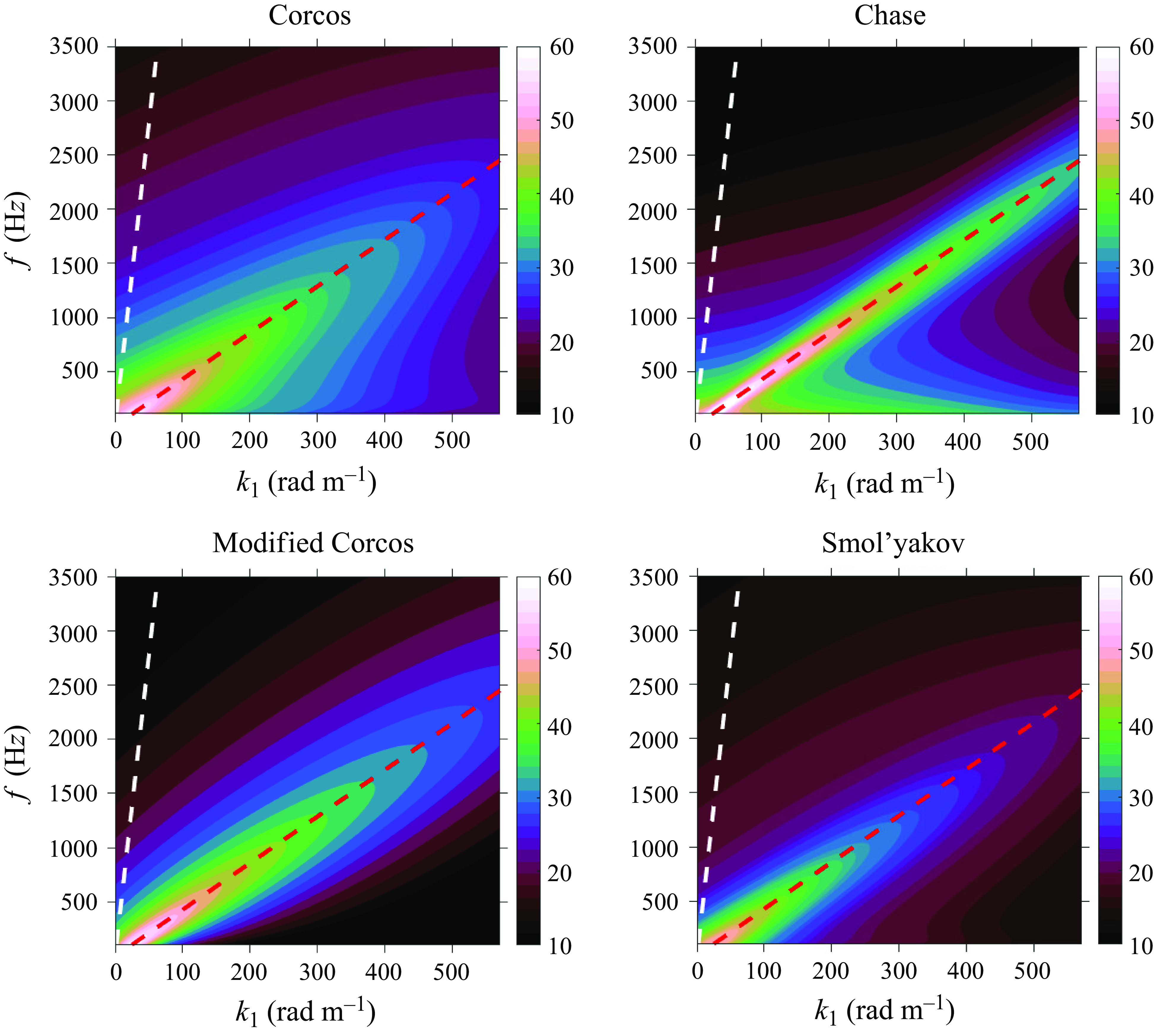
Figure 19. Wavenumber–frequency spectrum estimates from various models for the array of sensors.

Figure 19 illustrates the predicted wavenumber–frequency spectrum based on the four models described in $\S$ 2. The models do not account for acoustics, hence the absence of the acoustic regime. The axes and colour scale ranges of the contours are kept consistent with the measured data plot (figure 18), which makes comparison with the measured data appropriate. The non-dimensional axes are avoided here to prevent visual clutter; however, the same axes as in figure 18 apply, along with the colour bar scaling. Figure 19 shows that the models capture the convective ridge; however, there are discrepancies. Most wall pressure models show a symmetric convective ridge. This unrealistic symmetry persists even if the models are run with the observed variable, convection velocity. This suggests the need for modifications to the convective ridge models. The Corcos and Smol’yakov models show very similar behaviour, with the Smol’yakov model showing lower overall levels. This is mainly due to their same overall form, with differences in modelling the correlation length scales. Both models show a broad convective ridge with a smoother transition into the sub-convective regime, in contrast to the measured data. Figure 18 shows a frequency-dependent convective ridge, whereas the models assume a fixed convection ratio ( $U_c/U_e = 0.7$ ). The Chase model aligns closely with the measured data and shows a tightly constrained convective ridge similar to the measurements. This has further relevance as the array design was based on the modified Corcos model, and the flow data show a larger overlap with the Chase model, indicating independence in the choice of model. It also shows that the measured data truly capture the flow dynamics. An interesting observation for the Chase model prediction is the broadening observed as frequencies approach zero. This is due to the dependence of the model’s cross-spectral density function on $\omega ^{-1}$ . Such a broadband behaviour is not observed in the measured data.

The modified Corcos model introduces variations in the convective ridge compared to the original Corcos and Smol’yakov models, allowing the ridge to narrow, aligning more closely with the measured data. However, the transition to the sub-convective regime shows a slow decay of levels, which is not observed in the data. The Chase model estimates a symmetric convective ridge; however, the data show an asymmetric ridge with slower decay at higher wavenumbers. The sub-convective behaviour predicted by Chase tends towards a complex, wavenumber-dependent form at lower wavenumbers, consistent with the measured data. Generally, Chase has the lowest levels, Corcos overpredicts, Smol’yakov underpredicts, and the modified Corcos is the best of Corcos and Smol’yakov. Moreover, the sub-convective regime levels predicted by the models are higher than the measured data, indicating a need for wall pressure model adjustments.

Figure 20 compares the measured data and the model predictions through horizontal slices of the wavenumber–frequency spectrum. The spectrum is normalised on the autospectrum of the sensor to account for area averaging. The $x$ -axis is normalised on the nominal convective wavenumber ( $k_c=\omega /U_c$ ) to align the convective peaks. Fixed frequencies $\omega \delta ^*/U_{\infty }=1$ and 2 are chosen for the comparison. Wavenumbers with $k_1/k_c\lt 1$ correspond to the sub-convective regime. The convective peak aligns well for the models due to a constant convective relation; however, the measured data observe a shift in the peak due to frequency-dependent convective speed. Differences are observed in the levels and the width of the convective peak. The levels for the modified Corcos and Chase models agree best with the measurements, while for others, these are underpredicted. There is a distinct difference in the convective peak shape for different cases. The measurements exhibit a much faster roll-off into the sub-convective ridge than all models except Chase, with peak slope $124.5\ \text{dB}/(k_1/k_c)$ in the measurements compared to $25.5\ \text{dB}/(k_1/k_c)$ in the modified Corcos model. Among all models, the Chase model predicts the lowest levels in the sub-convective regime; however, it falls above the measured data by 5–10 dB. This inconsistency can be attributed to modelling assumptions in $\S$ 3.1 and the inaccuracies in wall pressure models. The measured data (red) also show a rise in levels at very small wavenumbers ( $k_1/k_c\lt 0.1$ ), corresponding to the acoustic cone. The Corcos and Smol’yakov models overpredict the levels by 10–15 dB in the sub-convective regime, and show a broad convective ridge. None of the models captures the asymmetry in the convective ridge observed in the measurements.

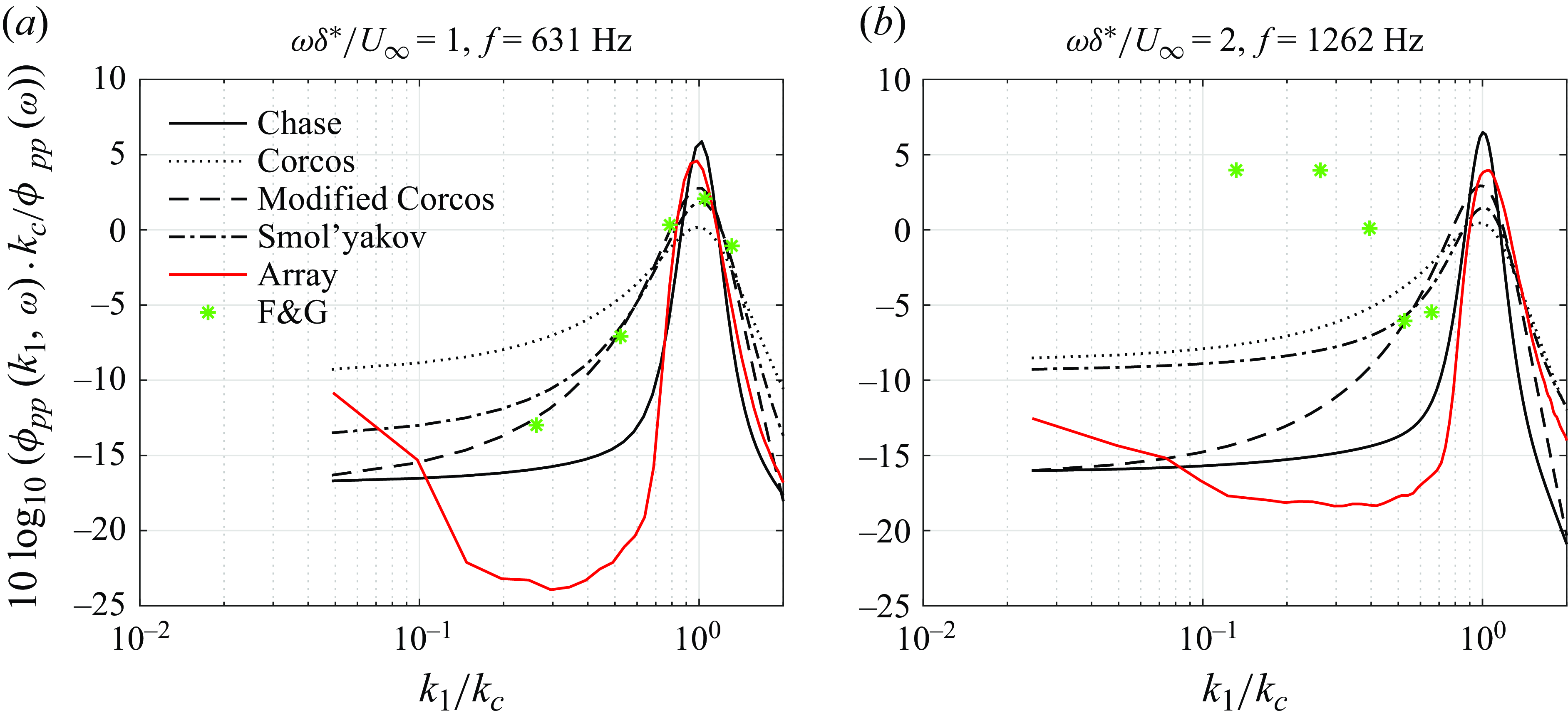
Figure 20. Frequency slices from the measured and estimated wavenumber–frequency spectra.

Figure 21 presents two vertical slices of the wavenumber–frequency spectrum normalised on boundary layer parameters ( $\delta ^*, U_\infty , \tau _w$ ). Normalised wavenumbers $k_1\delta ^*=0.42$ and 0.76 are chosen for comparisons. The convective peak levels agree for all models (within $\pm 2$ dB) except the Smol’yakov model. There is a difference in the peak location due to the frequency dependence of the convection velocity. The region on the right-hand side of the convective peak is the sub-convective region. The Chase model predicts significantly lower levels in the sub-convective domain than the other models. These predictions are close to the measured array data, but there are some differences observed, including the transition to the sub-convective regime ( $\omega \delta ^*/U_{\infty }\gt 0.3$ for the $k_1\delta ^*=0.42$ slice). The measured data (red) show a rise in levels towards higher frequencies ( $\omega \delta ^*/U_{\infty }\gt 2$ for the $k_1\delta ^*=0.42$ slice); while this may well be real, it also might represent the impact of the residual high frequency low-wavenumber aliasing error visible in figure 8(b). The Smol’yakov model has an overall profile similar to the array data in the sub-convective regime, although it severely underpredicts the convective peak. This could imply a mixed-length correlation factor for wall pressure model improvements due to the Smol’yakov model using mixed-length correlations (2.17) instead of separating the spanwise and streamwise correlations as done by the Corcos and modified Corcos models. The Corcos and modified Corcos models agree near the convective peak but diverge in the sub-convective regime, with a variation within 5 dB. At higher wavenumbers, the trends are consistent with low-wavenumber behaviour.

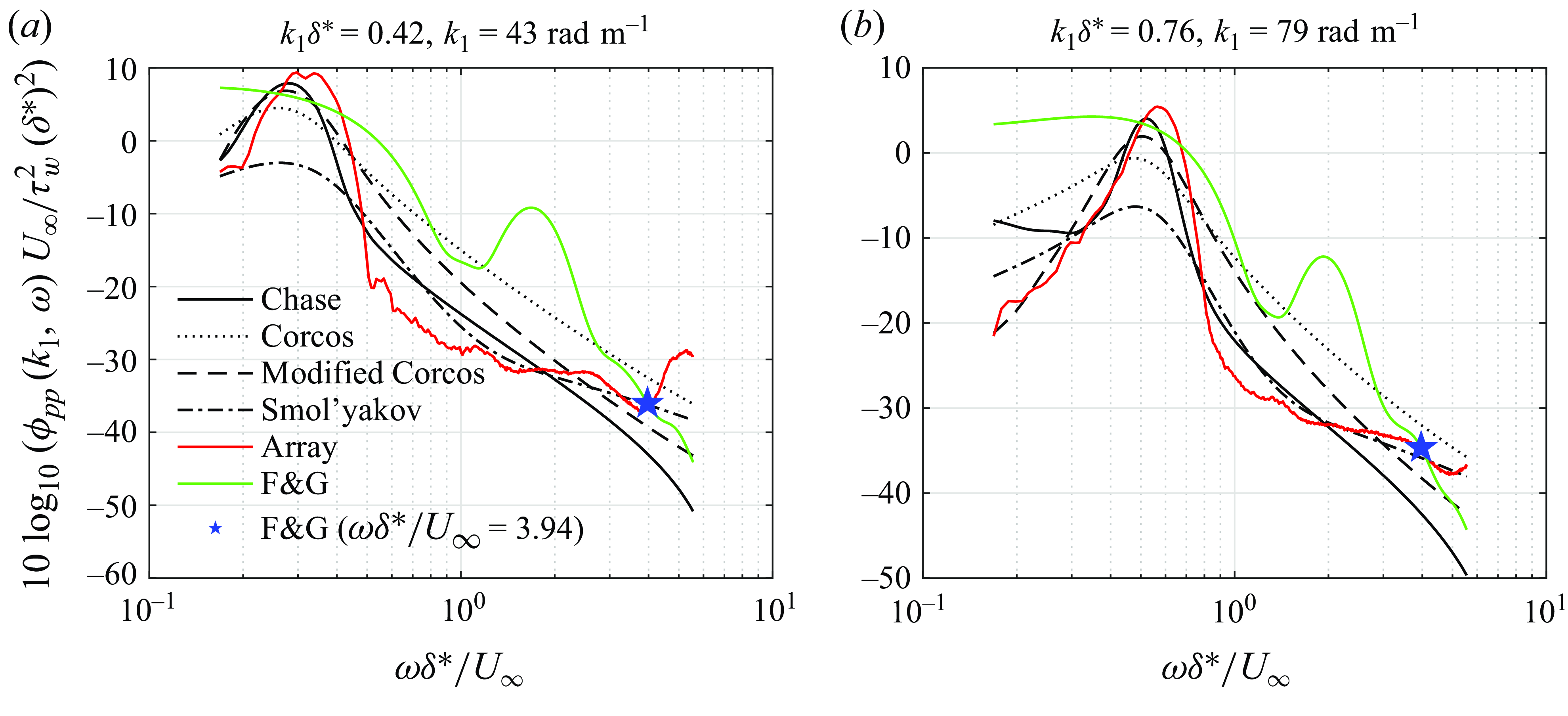
Figure 21. Wavenumber slices from the measured and estimated wavenumber-frequency spectra.

Figures 20 and 21 compare the F&G array data (green) with the sub-resonant sensor array data (red). In interpreting these plots, it is important to remember that Farabee & Geib (1991) identified a single wavenumber–frequency point ( $k_1 \delta ^*=1.12,\ \omega \delta ^*/U_\infty =3.94$ ) to reveal the sub-convective levels based on the analogue data processing system available at the time. Here, all possible wavenumbers and frequencies have been identified based on the discrete Fourier transform algorithms available today. Figure 20 presents the frequency slice for the F&G array. Despite differences in sensor areas, normalisation on the autospectrum ensures some comparability. The F&G array exhibits a broadened convective peak due to limited wavenumber resolution and spatial aliasing, with sub-convective levels at least 10 dB higher than the sub-resonant array measured data. A coincidental agreement is observed in figure 20(a) at $k_1/k_c \approx 0.8$ . For the wavenumber slices shown in figure 21, one can clearly identify the broadened convective peak and the aliased bump at slightly higher frequencies. Beyond the aliased bump, the frequency ( $\omega \delta ^*/U_\infty =3.94$ ) is shown with a blue star, indicating the point where the levels can be trusted. At $ k_1 \delta ^*= 1.12$ ( $ k_1 = 116.7$ rad m⁻¹) and $ \omega \delta ^*/U_\infty = 3.94$ (2.5 kHz), F&G data were 0.5 dB above the array levels, a difference likely suppressed by aliasing of sub-resonant array measurements. These results demonstrate the limitations of sparse microphone arrays in resolving sub-convective pressure fluctuations while confirming an agreement between the new sub-resonator-based sensor array and the F&G array. To the best of our knowledge, all comparisons shown in the preceding section uncover the gaps in sub-convective pressure levels between experiments and models. This also serves as a validation of the Chase (1980) model, which has been difficult in the past. This attests to the measurement technique and uncovers possibilities in wall pressure modelling.

6. Conclusions

This study presents a novel measurement technique for the measurement of sub-convective pressure fluctuations in turbulent boundary layers. Sensors with a high aspect ratio, large area ( $0.75\delta \times 0.075\delta$ ) aligned perpendicular to the flow are chosen to filter convective pressure fluctuations, and their arrangement in space is optimised by a mathematical modelling approach. An array of 80 multi-pore Helmholtz resonator-based sensors comprising an acoustic cavity, rigid flow interface with pores and a microphone is used to measure the wall pressure fluctuations. A detailed comparison is conducted between existing wall pressure models and wind tunnel data on sub-convective pressure fluctuations for a near-zero pressure gradient condition. The models used include incompressible (Corcos 1967; Chase 1980; Smol’yakov 2006) and modified Corcos (Hwang et al. 2003). The sensor area sensitivity is approximated as a spatial summation of weighted delta functions based on the discrete distribution of pores over the sensor area.

Measurements were conducted for long sampling durations, and a convergence study showed a drop in coherence levels as low as $-45$ dB with an increase in sampling duration from $7 \times 10^5\delta ^*/U_\infty$ to $10^7\delta ^*/U_\infty$ . This conveyed the need for long temporal scales to resolve the sub-convective fluctuations, as observed by Abtahi et al. (2024a ). This inference is crucial due to its implications on the cost of computational studies and data requirements of large-scale measurements. The cross-spectrum was studied as a function of frequency and streamwise separation, showing an exponential decay, as often modelled. A side-lobe-type behaviour was observed due to a surprising compactness of the convective ridge in the wavenumber domain. A continuous wavenumber–frequency spectrum was obtained using the array of sensors, showing a distinction between the supersonic, sub-convective and convective ridge. The spectrum revealed sufficient range and resolution in the sub-convective domain. It covered a range of wavenumbers ( $0\lt k_1\delta ^*\lt 11$ ) and frequencies ( $0.16\lt \omega \delta ^*/U_{\infty }\lt 5.5$ ). The convective ridge was observed to have an asymmetric behaviour about the convective line, with a sharp transition into the sub-convective domain. This reflects the physical nature of the flow, with no pressure disturbances other than sound occupying group speeds beyond the convective ridge. The convective speed was observed to be a function of frequency, with decreasing values at increasing frequencies.

Comparisons with the F&G array estimates reveal the inability of the large-sensor/small-array (F&G array) to resolve sub-convective pressure levels as low as in the array developed in this study. However, some agreements with the measured data validate the results and suggest that the results from Farabee & Geib (1991) were truly remarkable for their capabilities. Comparisons with wall pressure models show some agreement at a range of frequencies, but large discrepancies exist. All models except Chase underpredict the cross-spectral levels and overpredict the correlation decay rate. The Chase model captures the sharp transition from the convective ridge to the sub-convective domain in the wavenumber–frequency space. Measured levels in the sub-convective regime are less than in all models at lower frequencies, but higher at larger frequencies, indicating a difference in the dynamic range between the models and the measured data. The results suggest that an optimal model might combine the Chase and Smol’yakov models at lower and higher frequencies, respectively. Alternatively, this hints towards a modification of the Chase model accounting for the convective peak’s dependence on frequency and the asymmetry in the convective ridge.