Hostname: page-component-78c5997874-xbtfd Total loading time: 0 Render date: 2024-11-09T02:28:43.036Z Has data issue: false hasContentIssue false

On the low-frequency dynamics of turbulent separation bubbles

Published online by Cambridge University Press:  22 August 2024

C. Cura*
Affiliation:
Institut für Luft- und Raumfahrt, Technische Universität Berlin, 10587 Berlin, Germany
A. Hanifi
Affiliation:
FLOW, Engineering Mechanics, KTH Royal Institute of Technology, 100 44 Stockholm, Sweden
A.V.G. Cavalieri
Affiliation:
Divisão de Engenharia Aeronáutica, Instituto Tecnológico de Aeronáutica, 12228-900 São José dos Campos, SP, Brazil
J. Weiss
Affiliation:
Institut für Luft- und Raumfahrt, Technische Universität Berlin, 10587 Berlin, Germany
*
Email address for correspondence: c.cura@tu-berlin.de

Abstract

The low-frequency modal and non-modal linear dynamics of an incompressible, pressure-gradient-induced turbulent separation bubble (TSB) are investigated, with the objective of studying the mechanism responsible for the low-frequency contraction and expansion (breathing) commonly observed in experimental studies. The configuration of interest is a TSB generated on a flat test surface by a succession of adverse and favourable pressure gradients. The base flow selected for the analysis is the average TSB from the direct numerical simulation of Coleman et al. (J. Fluid Mech., vol. 847, 2018, pp. 28–70). Global mode analysis reveals that the eigenmodes of the linear operator are damped for all frequencies and wavenumbers. Furthermore, the least damped eigenmode appears to occur at zero frequency and low, non-zero spanwise wavenumber when scaled with the separation length. Resolvent analysis is then employed to examine the forced dynamics of the flow. At low frequency, a region of low, non-zero spanwise wavenumber is also discernible, where the receptivity appears to be driven by the identified weakly damped global mode. The corresponding optimal energy gain is shown to have the shape of a first-order, low-pass filter with a cut-off frequency consistent with the low-frequency unsteadiness in TSBs. The results from resolvent analysis are compared to the unsteady experimental database of Le Floc'h et al. (J. Fluid Mech., vol. 902, 2020, A13) in a similar TSB flow. The alignment between the optimal response and the first spectral proper orthogonal decomposition mode computed from the experiments is shown to be close to $95\,\%$, while the spanwise wavenumber of the optimal response is consistent with that of the low-frequency breathing motion captured experimentally. This indicates that the fluctuations observed experimentally at low frequency closely match the response computed from resolvent analysis. Based on these results, we propose that the forced dynamics of the flow, driven by the weakly damped global mode, serve as a plausible mechanism for the origin of the low-frequency breathing motion commonly observed in experimental studies of TSBs.

Type
JFM Papers
Copyright
© The Author(s), 2024. Published by Cambridge University Press

1. Introduction

Flow separation is a common phenomenon within fluid dynamics, which arises when a fluid flow is no longer able to follow the trajectory imposed by a solid wall. Separated flows exhibit a variety of detrimental effects, including reduced lift, increased drag, noise emission and vibrations, all of which may negatively impact the performance of the system under consideration. A distinct subset within separated flows is the category of reattaching flows, where the flow reattaches to the wall, e.g. due to surface curvature or a favourable pressure gradient. This category gives rise to so-called separation bubbles, which are known to feature unsteadiness in a variety of spatial and temporal scales. In the present contribution, we specifically consider turbulent separation bubbles (TSBs), which occur when a turbulent boundary layer separates from the wall and reattaches further downstream. We further focus our study on pressure-gradient-induced TSBs, where detachment from a smooth surface occurs because of an adverse pressure gradient (Na & Moin Reference Na and Moin1998). This is in contrast to flows where the separation line is fixed by the surface geometry (Eaton & Johnston Reference Eaton and Johnston1981).

Unsteadiness in pressure-induced TSBs typically occurs in three broad ranges of frequencies that may be categorized by their Strouhal number $St=f L_b/U_{ref}$ based on the separation length $L_b$ and a reference velocity $U_{ref}$ (Mabey Reference Mabey1972). For relatively high values $St > 1$, fluctuations are caused mainly by turbulent motions that have their highest amplitude in the attached flow upstream and downstream of the backflow region (Abe Reference Abe2017; Le Floc'h et al. Reference Le Floc'h, Weiss, Mohammed-Taifour and Dufresne2020; Wu, Meneveau & Mittal Reference Wu, Meneveau and Mittal2020). Within the recirculation zone, medium frequencies centred at $St \approx 0.1\unicode{x2013}1.0$ appear in the wall-pressure and velocity fields due to the roll-up and shedding of vortices originating in the shear layer (Kiya & Sasaki Reference Kiya and Sasaki1983; Cherry, Hillier & Latour Reference Cherry, Hillier and Latour1984). Finally, a low-frequency unsteadiness, typically characterized by a large-scale contraction and expansion (‘breathing’) of the TSB, is often observed at $St \approx 0.01\unicode{x2013}0.1$ (Mohammed-Taifour & Weiss Reference Mohammed-Taifour and Weiss2016). This is the main focus of the present work.

To date, low-frequency unsteadiness in pressure-induced TSBs has been observed mostly in high-speed flows, where it often occurs within shockwave/boundary layer interactions (SBLIs) (Dolling Reference Dolling2001). There, the breathing of the TSB is associated with a low-frequency, aperiodic oscillation of a separation shock that can generate strong detrimental pressure and thermal loads on the structure, as described in the review articles by Dussauge, Dupont & Debiève (Reference Dussauge, Dupont and Debiève2006), Clemens & Narayanaswamy (Reference Clemens and Narayanaswamy2014) and Gaitonde (Reference Gaitonde2015). Recently, evidence of similar low-frequency unsteadiness has also been observed in subsonic flows. Weiss, Mohammed-Taifour & Schwaab (Reference Weiss, Mohammed-Taifour and Schwaab2015) and Mohammed-Taifour & Weiss (Reference Mohammed-Taifour and Weiss2016) experimentally set up a TSB on a flat test surface through the combination of adverse and favourable pressure gradients. They observed its low-frequency breathing at a Strouhal number similar to that of SBLIs ($St \approx 0.01$). Consistent findings were also reported by Richardson et al. (Reference Richardson, Zhang, Cattafesta and Wu2023) in a configuration that featured only an adverse pressure gradient (APG) but no favourable pressure gradient (FPG), by Weiss et al. (Reference Weiss, Steinfurth, Chamard, Giani and Combette2022) in a turbulent half-diffuser flow, and by Wang & Ghaemi (Reference Wang and Ghaemi2022) in the separation bubble on a two-dimensional airfoil. On the numerical side, Wu et al. (Reference Wu, Meneveau and Mittal2020) computed a configuration similar to Richardson et al. (Reference Richardson, Zhang, Cattafesta and Wu2023) via direct numerical simulation (DNS) but did not capture the low frequencies observed in the experiment. On the other hand, Larchevêque (Reference Larchevêque2020) showed good agreement between the characteristic frequency of the breathing motion ($St \approx 0.01$) of flat-plate TSBs at low-subsonic, high-subsonic, and supersonic flows based on large eddy simulations. This suggests that similar low-frequency behaviour occurs in a wide range of Mach numbers, as argued by Weiss et al. (Reference Weiss, Mohammed-Taifour and Schwaab2015, Reference Weiss, Little, Threadgill and Gross2021).

Proposed mechanisms for the occurrence of low-frequency unsteadiness in turbulent SBLIs (and, by association, subsonic TSBs) typically consist of two main categories (Clemens & Narayanaswamy Reference Clemens and Narayanaswamy2014): an upstream mechanism, whereby velocity fluctuations in the incoming boundary layer directly influence the position of the separation line and modulate the size of the TSB (Beresh, Clemens & Dolling Reference Beresh, Clemens and Dolling2002) – in this case, the low-frequency character of the unsteadiness is explained by the presence of very-large-scale turbulent structures that have been observed in both subsonic and supersonic boundary layers (Ganapathisubramani, Longmire & Marusic Reference Ganapathisubramani, Longmire and Marusic2003; Ganapathisubramani, Clemens & Dolling Reference Ganapathisubramani, Clemens and Dolling2007) – and a downstream mechanism, where the low-frequency unsteadiness is caused by inherent amplification in the TSB. In the latter hypothesis, both shear layer (Piponniau et al. Reference Piponniau, Dussauge, Debieve and Dupont2009) and centrifugal (Priebe et al. Reference Priebe, Tu, Rowley and Martín2016; Wu et al. Reference Wu, Meneveau and Mittal2020) mechanisms have been considered. Mohammed-Taifour & Weiss (Reference Mohammed-Taifour and Weiss2016) discussed the relevance of these hypotheses for the case of subsonic pressure-induced TSBs but could not find any conclusive evidence to select a suitable mechanism. More recently, a third, intermediate model of low-frequency unsteadiness was put forward by Porter & Poggie (Reference Porter and Poggie2019), who suggested that certain large-scale, near-wall perturbations in the incoming boundary layer may drive a weakly damped global mode of the separation bubble. This model inherently implies that a combination of both upstream and downstream elements is responsible for the low-frequency unsteadiness (the presence of perturbations upstream and the global mode downstream), and ‘reconciles the debate between upstream and downstream mechanisms of separation unsteadiness’ (Porter & Poggie Reference Porter and Poggie2019). Such an intermediate model is also consistent with the subsonic results of Mohammed-Taifour & Weiss (Reference Mohammed-Taifour and Weiss2021), who demonstrated experimentally that the low-frequency behaviour in their TSB is well illustrated by a first-order low-pass filter model that converts the broadband fluctuations of the incoming turbulent boundary layer into a low-frequency, large-scale oscillation of the separation and reattachment fronts.

Relevant frameworks for the study of low-frequency unsteadiness in separated flows are global mode analysis (GMA) and resolvent analysis (RA). Both approaches rely on a linearization of the equation of motion around a suitable base flow. In the case of GMA, the asymptotic behaviour of the homogeneous linear system is studied to reveal the presence of global modes of oscillations and their respective growth rates (Theofilis Reference Theofilis2003, Reference Theofilis2011). Positive growth rates suggest that inherent instabilities are present in the flow, which may then be qualified as an oscillator capable of sustaining self-excited oscillations without the presence of forcing. There are broad applications of GMA to study the stability of laminar solutions (Theofilis Reference Theofilis2011). When used with linearizations around the mean turbulent solution, it may also provide information on dominant oscillation frequencies (Barkley Reference Barkley2006; Schmidt et al. Reference Schmidt, Towne, Colonius, Cavalieri, Jordan and Brès2017), although this cannot be ensured a priori (Sipp & Lebedev Reference Sipp and Lebedev2007). On the other hand, for flows with solely damped modes, RA investigates the forced dynamics of the linearized flow by lumping all nonlinear terms that occur in the linearization process into a forcing term (Hwang & Cossu Reference Hwang and Cossu2010; McKeon & Sharma Reference McKeon and Sharma2010; Cavalieri, Jordan & Lesshafft Reference Cavalieri, Jordan and Lesshafft2019). The approach relies on the singular value decomposition (SVD) of the resolvent operator to identify the optimal forcing and its associated linear response. As such, RA may help to identify specific zones of amplification in the flow, even in the absence of any amplified global mode. When this occurs, such flows are typically characterized as amplifiers instead of oscillators (Huerre & Monkewitz Reference Huerre and Monkewitz1990).

To date, most global linear analyses of separation bubbles have been conducted at relatively low Reynolds numbers, in an attempt to describe the onset of unsteadiness and three-dimensionality in laminar separated flows. Following the seminal work of Theofilis, Hein & Dallmann (Reference Theofilis, Hein and Dallmann2000), several authors have demonstrated the existence of both oscillator- and amplifier-type dynamics in low-speed, two-dimensional laminar separation bubbles (e.g. Ehrenstein & Gallaire Reference Ehrenstein and Gallaire2008; Marquet et al. Reference Marquet, Sipp, Chomaz and Jacquin2008; Rodríguez & Gennaro Reference Rodríguez and Gennaro2017). At higher Mach numbers, the topic of low-frequency unsteadiness was specifically addressed by Robinet (Reference Robinet2007), who investigated the stability of a laminar SBLI through GMA, and demonstrated the appearance of a three-dimensional global instability when the angle of the incident shock was increased. The presence of low-frequency unsteadiness in laminar SBLIs was later confirmed by Sansica, Sandham & Hu (Reference Sansica, Sandham and Hu2016), who linked its appearance to the laminar/turbulent transition occurring in the separated shear layer, and suggested that ‘the separation bubble acts as a low-pass spatial amplification filter’. Consistent results were recently presented by Bugeat et al. (Reference Bugeat, Robinet, Chassaing and Sagaut2022), who related the low-frequency behaviour in a laminar SBLI to the excitation of a stable global mode. The optimal gain computed by RA resembled a first-order low-pass filter, thereby recovering the signature of low-frequency unsteadiness typically observed in turbulent SBLIs (Poggie et al. Reference Poggie, Bisek, Kimmel and Stanfield2015).

In turbulent flows, linear analyses may also be conducted by selecting the turbulent mean as base flow (Crow & Champagne Reference Crow and Champagne1971; Michalke Reference Michalke1984; Del Alamo & Jimenez Reference Del Alamo and Jimenez2006; Hwang & Cossu Reference Hwang and Cossu2010; McKeon & Sharma Reference McKeon and Sharma2010), although in this case the modal analysis of the linearized operator may not qualify as stability analysis since the mean flow does not satisfy the Navier–Stokes equations. Touber & Sandham (Reference Touber and Sandham2009) performed such a study on the mean flow obtained from the large eddy simulations of a turbulent SBLI, and found an amplified global mode that they suggested could be linked to the observed low-frequency unsteadiness. Consistent results were later obtained by Nichols et al. (Reference Nichols, Larsson, Bernardini and Pirozzoli2017) and Adler & Gaitonde (Reference Adler and Gaitonde2018), who also discovered a global amplified mode related to low-frequency unsteadiness in similar flow configurations. Through the use of linear analysis, Sasaki et al. (Reference Sasaki, Barros, Cavalieri and Larchevêque2021) suggested that upstream travelling acoustic waves are responsible for the low-frequency unsteadiness in a turbulent SBLI, thereby confirming a previous hypothesis by Pirozzoli & Grasso (Reference Pirozzoli and Grasso2006). While all these studies proposed that turbulent SBLIs behave as oscillators, the works of Sartor et al. (Reference Sartor, Mettot, Bur and Sipp2015) and Hao (Reference Hao2023) on a transonic and supersonic SBLI, respectively, indicated an amplifier behaviour for low-frequency perturbations. The latter conclusion was obtained by performing GMA and RA on the average flow computed by Reynolds-averaged Navier–Stokes (RANS) simulations. Similar to the results of Bugeat et al. (Reference Bugeat, Robinet, Chassaing and Sagaut2022) in a laminar SBLI, Hao (Reference Hao2023) related the low-frequency unsteadiness to the excitation of an intrinsic mode by external disturbances.

In this framework, the objective of the present study is to investigate the low-frequency unsteadiness of an incompressible, pressure-gradient-induced TSB by means of GMA and RA. Specifically, we address the upstream/downstream dichotomy by examining the characteristics of global modes and their responses to external perturbations, with the aim to better understand the mechanism causing the low-frequency breathing. From a practical perspective, our motivation is threefold: first, subsonic TSBs may serve as a reference for more complex turbulent SBLIs, where low-frequency unsteadiness is often detrimental to flight performance; second, smooth-body flow separation remains a challenge for industrial RANS turbulence models, which may require specific treatment for low-frequency unsteadiness; and finally, to our knowledge, such an analysis has not yet been performed in the fluid dynamics community.

The configuration that we consider is a TSB generated on a flat test surface by a combination of APGs and FPGs. Such a flow has already been investigated experimentally by Le Floc'h et al. (Reference Le Floc'h, Weiss, Mohammed-Taifour and Dufresne2020) and numerically via DNS by Coleman, Rumsey & Spalart (Reference Coleman, Rumsey and Spalart2018). Our chosen methodology is to perform the linear analysis on a base flow consisting of the average DNS flow field, and to validate the GMA and RA results with the unsteady experimental database. As will be seen in the following sections, this cross-validation between two separate databases strongly supports the relevance of our findings.

The paper is organized as follows. In § 2, we introduce the experimental database and demonstrate the existence of low-frequency unsteadiness from both fluctuating velocity and wall-pressure data. Then in § 3, we describe our chosen base flow and discuss its relevance to the present investigation. The methodology for GMA and RA is introduced in § 4, and the corresponding results are presented in § 5. These results are then compared to the experimental database and other studies in § 6, before a conclusion is offered in § 7. Specific details about the linear analysis are provided in appendices.

2. Experimental database

In this section, we introduce the unsteady experimental database of Le Floc'h et al. (Reference Le Floc'h, Mohammed-Taifour, Dufresne and Weiss2018, Reference Le Floc'h, Weiss, Mohammed-Taifour and Dufresne2020) that will be used in the present study. We briefly discuss the wind tunnel set-up, after which we proceed to outline the unsteady characteristics of the flat-plate TSB, with a specific emphasis on low-frequency unsteadiness.

2.1. Experimental set-up

The experiments of Le Floc'h et al. (Reference Le Floc'h, Mohammed-Taifour, Dufresne and Weiss2018, Reference Le Floc'h, Weiss, Mohammed-Taifour and Dufresne2020) were conducted in the TFT boundary-layer wind tunnel, a low-speed, blow-down facility designed specifically for the study of TSBs (Mohammed-Taifour et al. Reference Mohammed-Taifour, Schwaab, Pioton and Weiss2015). The wind tunnel features a test section measuring $3\,{\rm m}$ in length and $0.6\,{\rm m}$ in width. A combination of APG and FPG is generated through the widening and subsequent converging test-section floor. Whereas the APG causes the incoming zero pressure gradient (ZPG) flat-plate turbulent boundary layer on the upper surface to separate, a boundary-layer bleed is located on the test-section floor to ensure that the flow on the lower surface remains attached. The FPG then forces the shear layer to reattach on the upper test surface, leading to the formation of a closed TSB. All experiments were performed at reference velocity $U_{ref}=25\,{\rm m}\,{\rm s}^{-1}$, and the Reynolds number of the incoming ZPG boundary layer (based on momentum thickness $\varTheta _{in}=3\,{\rm mm}$) was approximately 5000.

Le Floc'h et al. (Reference Le Floc'h, Weiss, Mohammed-Taifour and Dufresne2020) investigated TSBs of different sizes by varying the streamwise distance between the APG and FPG. Here, we focus primarily on their medium TSB, which, as will be shown in the next section, is the closest to the flow studied numerically by Coleman et al. (Reference Coleman, Rumsey and Spalart2018). The length of the medium TSB, defined as the streamwise distance between the average separation and reattachment points on the test-section centreline, is $L_b = 0.11\,{\rm m}$. The experimental database of Le Floc'h et al. (Reference Le Floc'h, Weiss, Mohammed-Taifour and Dufresne2020) includes planar (two-dimensional) time-resolved particle image velocimetry (TR-PIV) in the streamwise/wall-normal plane as well as unsteady wall-pressure measurements on the centreline of the test section. To illustrate the spanwise character of the low-frequency unsteadiness, these results will be complemented with unsteady wall-pressure measurements in the spanwise direction by Le Floc'h et al. (Reference Le Floc'h, Mohammed-Taifour, Dufresne and Weiss2018) and near-wall TR-PIV measurements in the streamwise/spanwise plane of the large TSB. The latter are unpublished data from Mohammed-Taifour & Weiss (Reference Mohammed-Taifour and Weiss2016).

A schematic representation of the wind-tunnel test section, with the mean streamwise velocity field measured on the centreline, is depicted in figure 1. Here, $H_0$ and $H_1$ indicate the approximate positions of the near-wall TR-PIV planes, whereas $x_1$ and $x_2$ are the streamwise positions of wall-pressure measurements (see § 2.2). While the $y$-axis was oriented towards the ground during the experiments, in the remainder of the paper we will switch the $y$-direction towards the top of the page. Required descriptions of the measurement techniques will be provided in the following sections as needed. More details on the experiments may be obtained in the original publications by Mohammed-Taifour & Weiss (Reference Mohammed-Taifour and Weiss2016) and Le Floc'h et al. (Reference Le Floc'h, Mohammed-Taifour, Dufresne and Weiss2018, Reference Le Floc'h, Weiss, Mohammed-Taifour and Dufresne2020).

Figure 1. Schematic of wind tunnel test section with mean streamwise velocity field on the centreline. The time-averaged TSB is indicated by the dividing streamline $\bar {\varPsi }=0$ (solid white line). Here, $H_0$ and $H_1$ indicate the approximate position and width of the near-wall TR-PIV measurements in the ($x\unicode{x2013}z$) plane. Note that the thickness of the indicated PIV planes is representative only and thus not true to scale.

2.2. Evidence of low-frequency unsteadiness

We start by employing spectral proper orthogonal decomposition (SPOD), first introduced by Lumley (Reference Lumley1970), to characterize the low-frequency breathing of the TSB. As opposed to the ‘classical’ and ‘snapshot’ POD commonly found in the recent literature, SPOD produces modes that oscillate at a single frequency (Towne, Schmidt & Colonius Reference Towne, Schmidt and Colonius2018). It is therefore a robust and powerful tool for analysing low-frequency unsteadiness, as demonstrated for instance by the recent results of Weiss et al. (Reference Weiss, Steinfurth, Chamard, Giani and Combette2022) and Richardson et al. (Reference Richardson, Zhang, Cattafesta and Wu2023). In practice, we use the algorithm proposed by Towne et al. (Reference Towne, Schmidt and Colonius2018) that is based on Welch-type averaging for stationary random processes.

In figure 2, we display the streamwise and wall-normal components $\hat {u}$ and $\hat {v}$ of velocity fluctuations of the leading SPOD mode, computed from the TR-PIV measurements of Le Floc'h et al. (Reference Le Floc'h, Weiss, Mohammed-Taifour and Dufresne2020). The PIV field of view is $225\,{\rm mm}\times 75\,{\rm mm}$ ($x\unicode{x2013}y$) with sampling frequency $f_s=900\,{\rm Hz}$. The database consists of six successive time series of $N_t=3580$ snapshots each. Hence the decomposition is performed on a total of $N_t=21\,480$ PIV snapshots that are split in $72$ blocks of $N_{FFT}=512$ snapshots with $50\,\%$ overlap. Overlapping blocks between two consecutive (uncorrelated) runs are removed. This procedure results in a frequency resolution of $1.76\,{\rm Hz}$.

Figure 2. Leading SPOD mode, computed based on planar PIV measurements with $f_{s}=900\,{\rm Hz}$. The (a,c,e,g) streamwise $\hat {u}$ and (b,d,f,h) wall-normal component $\hat {v}$ are shown. The depicted frequencies, from top to bottom, correspond to (a,b) $St=0.01$, (c,d) $St=0.08$, (e,f) $St=0.11$, (g,h) $St=0.27$. The time-averaged location of the TSB is indicated by the dividing streamline $\bar {\varPsi }=0$ (black dashed line).

The real part of the leading mode is depicted for different Strouhal numbers $St=fL_b/U_{ref}$. A Strouhal number $St=0.01$, typically representing the low-frequency regime, is depicted in figures 2(a,b), whereas the remaining Strouhal numbers increase from top to bottom according to $St=0.08$ (figures 2c,d), $St=0.11$ (figures 2e,f) and $St=0.27$ (figures 2g,h). As will be discussed later (see figure 19), the first SPOD mode is particularly dominant at low frequency, with approximately $72\,\%$ of the energy density at $St = 0.01$. Note that the time-averaged location of the TSB is indicated by the dividing streamline (black dashed line) in the different plots.

In the low-frequency regime ($St= 0.01$), the streamwise component of the mode $\hat {u}$ features a large coherent structure that bounds the TSB and follows its shape. This behaviour can be observed for any low Strouhal number with $St\approx 0.01$. A similar, large-scale mode was first observed in the snapshot POD of the streamwise velocity component in Mohammed-Taifour & Weiss (Reference Mohammed-Taifour and Weiss2016). In their study, a low-order model was employed to show that this mode can be interpreted as a low-frequency contraction and expansion (breathing) of the TSB. More recently, SPOD has been applied to several pressure-induced TSB flows, and large-scale coherent structures similar to that depicted in figures 2(a,b) have been identified as the leading low-frequency SPOD mode for TSBs occurring in a one-sided diffuser (Steinfurth, Cura & Weiss Reference Steinfurth, Cura and Weiss2022), behind a wall-mounted hump (Dau et al. Reference Dau, Borgmann, Little and Weiss2023), and on a flat-plate with APG (Richardson et al. Reference Richardson, Zhang, Cattafesta and Wu2023). In all of these works, the aforementioned mode was associated with the low-frequency breathing of the TSB. In contrast, higher-frequency modes are qualitatively distinct: There, we observe an alternating pattern of coherent structures of opposite phase, which, in the literature, is often associated with the shedding of vortices from the shear layer bounding the recirculation region (e.g. Rajaee, Karlsson & Sirovich Reference Rajaee, Karlsson and Sirovich1994). When computing the phase speed $u_{ph}=\omega /k$ of the streamwise component of the complex SPOD modes, we obtain $u_{ph}\approx 0.3U_{ref}$ for $St\ge 0.08$. Here, $\omega =2{\rm \pi} f$ and $k=\partial \vartheta /\partial x$ is the streamwise wavenumber based on the phase $\vartheta$ extracted at $y\approx 0.04\,{\rm m}$. This value is consistent with the convection velocity $u_c=0.33U_{ref}$ of vortices observed in the DNS of Na & Moin (Reference Na and Moin1998) and in the experiments of Mohammed-Taifour & Weiss (Reference Mohammed-Taifour and Weiss2016). The corresponding wall-normal component of the modes conveys similar trends. While in the low-frequency regime, we observe structures that encompass a significant portion of the PIV domain, an increase in the Strouhal number results in a greater number of structures as well as smaller individual structure size.

Figure 2(a) indicates that at low frequency, the TSB contracts and expands in the streamwise direction (see also the discussion in the original article by Le Floc'h et al. Reference Le Floc'h, Weiss, Mohammed-Taifour and Dufresne2020). In order to estimate the spanwise scale of this motion, we now consider TR-PIV measurements performed in the streamwise/spanwise plane at elevation $y \approx 4\,{\rm mm}$ away from the wall (for reference, the boundary-layer thickness at position $H_0$ is approximately 30 mm). These measurements were performed in the large TSB of Mohammed-Taifour & Weiss (Reference Mohammed-Taifour and Weiss2016) (unpublished data; see also Mohammed-Taifour Reference Mohammed-Taifour2017). The PIV field of view is $75\,{\rm mm} \times 215\,{\rm mm}$ ($x\unicode{x2013}z$) with sampling frequency $f_s=900\,{\rm Hz}$.

The frequency–wavenumber spectra of the streamwise velocity fluctuations are depicted in figure 3. Two exemplary streamwise positions are chosen, representing the spanwise ($x\unicode{x2013}z$) planes ${H_0}$ (figure 3a) and $H_1$ (figure 3b). Here, $H_0$ is a plane in the ZPG region upstream of the TSB, and $H_1$ corresponds to a plane immediately upstream of the time-averaged location of the separation line; see figure 1. To extract the frequency–wavenumber spectra, we first perform a fast Fourier transform in the spanwise ($z$) direction on $N_t=3580$ snapshots of the fluctuating velocity $u'$ (e.g. Towne et al. Reference Towne, Cavalieri, Jordan, Colonius, Schmidt, Jaunet and Brès2017). We further compute the power spectral density (PSD) of the Fourier-transformed signal $\hat {u}$, adopting Welch's estimate using $50\,\%$ overlap. We obtain a spectrum for each streamwise position $x$. Here, the frequency is represented as the Strouhal number $St=f L_b/U_{ref}$, and the non-dimensional spanwise wavenumber is $\beta =(2{\rm \pi} L_b)/\lambda _z$. The chosen position corresponds to the centre of each PIV measurement plane, respectively. Similar results were obtained for all investigated positions within the planes $H_0$ and $H_1$. For visualization purposes, the PSD of $\hat {u}$ is scaled by a factor of $10$ for the $H_0$ plane in the upstream boundary layer (figure 3a).

Figure 3. Frequency–wavenumber spectrum of fluctuating velocity $u'$ in the $x\unicode{x2013}z$ plane at $y\approx 4\,{\rm mm}$ from the test surface. Two streamwise positions $x$ are depicted: (a) a position in the ZPG region upstream of the TSB, $x=1.33\,{\rm m}$, and (b) a position immediately upstream of the time-averaged location of the separation line, $x=1.68\,{\rm m}$. The spanwise wavenumber $\beta =2{\rm \pi} /\lambda _{z}$ is non-dimensionalized by the average bubble length $L_b$. The PSD in the ZPG region (a) is multiplied by a factor of $10$.

In the upstream ZPG boundary layer ($H_0$ plane), the maximum of the PSD of $\hat {u}$ is obtained for the non-dimensional spanwise wavenumber $\beta =\pm 65$ and Strouhal number range $St\le 0.8$ (figure 3a). All frequencies $St$ in the vicinity of $\beta =\pm 65$ exhibit fairly high energy levels. However, no substantial energy content can be detected in the region of two-dimensional perturbations $\beta =0$. Moreover, since the spectrum is symmetrical with respect to $\beta =0$, no preferential $z$-direction can be detected for the present configuration. This indicates that perturbations are equally likely to propagate in the $+z$ and $-z$ directions. When expressed in terms of the boundary-layer thickness $\delta =28\,{\rm mm}$ of the incoming turbulent flow (measured at $x=1.1\,{\rm m}$), the spanwise wavelength $\lambda _z$, related to the non-dimensional spanwise wavenumber $\beta =\pm 65$, is approximately $\lambda _z=0.4\delta$. This value is in agreement with the values of $ {O}(\delta )$ reported for the superstructures in the upstream boundary layer of several turbulent boundary layer flows (e.g. Tomkins & Adrian Reference Tomkins and Adrian2003; Hutchins & Marusic Reference Hutchins and Marusic2007; Le Floch et al. Reference Le Floc'h, Mohammed-Taifour, Weiss, Dufresne, Vétel and Jondeau2016). Interestingly, a similar organization of elongated structures over the span of the $H_0$ measurement plane can also be observed on the first SPOD modes at low frequency (not shown here).

In figure 3(b), we display the representative frequency–wavenumber spectrum of the measurement plane $H_1$. The majority of the energetic content is now gathered in the range $-2\le \beta \le 2$. Once again, the distribution is symmetrical with respect to $\beta =0$, indicating no preferential $z$-direction. On the other hand, the wavelengths $\lambda _z$ associated with the structures of this low-$\beta$ range are now large compared to the bubble length $L_b$. They take values between $\lambda _z=3L_b$ for $\beta =\pm 2$, to $\lambda _z\gg 10L_b$ for very small $\beta$. Hence the low-frequency unsteadiness of the TSB appears to be coherent over a large spanwise scale. Furthermore, the high-$\beta$ signature observed in the incoming ZPG boundary layer is absent from the frequency–wavenumber spectrum close to the separation line, thereby suggesting that the TSB is not responding directly to the long superstructures present in the incoming boundary layer.

To confirm these results, we now consider fluctuating wall-pressure data gathered in the spanwise direction by Le Floc'h et al. (Reference Le Floc'h, Mohammed-Taifour, Dufresne and Weiss2018) in the medium TSB again. All pressure signals were obtained by using piezoresistive pressure transducers with range $1$ psi ($6.89\,{\rm kPa})$ and estimated error ${\pm }5\,\%$. To eliminate low-frequency wind-tunnel noise in the signals, the correction method from Weiss et al. (Reference Weiss, Mohammed-Taifour and Schwaab2015) was applied. The PSD was calculated by adopting Welch's method using $50\,\%$ overlap and a Hamming window.

In figures 4(a,b), the classical log-log PSD and the pre-multiplied PSD of the fluctuating wall pressure $p'$ on the test-section centreline at two streamwise positions are shown, respectively: a position immediately upstream of the time-averaged location of the separation bubble ($x_1=1.60\,{\rm m}$), and a position in the region downstream of the TSB ($x_2=2.05\,{\rm m}$). These streamwise positions are depicted schematically in figure 1. The low-frequency unsteadiness becomes apparent as a distinct ‘hump’ in the pre-multiplied distribution for $x_1=1.60\,{\rm m}$, where a significant amount of energy is gathered in the region $St\approx 0.01$. This hump has also been observed by Mohammed-Taifour & Weiss (Reference Mohammed-Taifour and Weiss2016) and Richardson et al. (Reference Richardson, Zhang, Cattafesta and Wu2023), and has been associated with the low-frequency breathing of their TSB. On the other hand, a different behaviour can be observed for $x_2=2.05\,{\rm m}$. Here, a distinct peak is visible in the pre-multiplied PSD for $St\approx 0.1$. In Cura, Hanifi & Weiss (Reference Cura, Hanifi and Weiss2023), this medium-frequency unsteadiness was linked to convective amplification in the shear layer bounding the recirculation region.

Figure 4. (a) The PSD and (b) the pre-multiplied PSD of fluctuation pressure $p'$ for $x_1=1.60\,{\rm m}$ (black) and $x_2=2.05\,{\rm m}$ (blue). The Strouhal number $St$ is calculated based on the bubble length $L_b$ and the reference velocity $U_{ref}=25\,{\rm m}\,{\rm s}^{-1}$.

Returning to the spanwise characteristics of low-frequency unsteadiness, we show in figure 5(a) the two-point cross-correlation coefficient at zero time lag measured by Le Floc'h et al. (Reference Le Floc'h, Mohammed-Taifour, Dufresne and Weiss2018). Here, $R_{p'p'}=\overline {p'(z)*p'_{ref}(z_{ref})}/(p'_{rms}*p'_{ref,rms})$ was obtained by simultaneously measuring the wall-pressure fluctuations at the centreline of the test section ($z_{ref}=0\,{\rm mm}$) and with a moving sensor positioned successively at $z=[0, \pm 0.05, \pm 0.10, \pm 0.15, \pm 0.20]$ m along the span of the wind-tunnel test section. Furthermore, all pressure signals were low-pass filtered to frequencies below $St = 0.03$ before computing the cross-correlations, so that only values that correspond to the low-frequency hump in figure 4 are considered. Again, two streamwise positions, $x_1=1.60\,{\rm m}$ and $x_2=2.05\,{\rm m}$, are depicted. In both cases, a wave-like distribution of $R_{p'p'}$ over the span, with a relatively large wavelength $\lambda _z$, becomes apparent. This confirms that the low-frequency unsteadiness is coherent over a large portion of the test-section span.

Figure 5. (a) Spanwise correlation $R_{p^\prime p^\prime }$ of low-pass filtered fluctuating pressure for two streamwise positions, $x_1=1.60\,{\rm m}$ (squares) and $x_2=2.05\,{\rm m}$ (circles) modified from Le Floc'h et al. (Reference Le Floc'h, Mohammed-Taifour, Dufresne and Weiss2018). (b) Cosine fit $f(z)=c_1 \cos (c_2z)$ of $R_{p^\prime p^\prime }$ (solid line) at $x_1=1.60\,{\rm m}$. The resulting non-dimensional spanwise wavenumber $\beta = (2{\rm \pi} L_{b})/\lambda _{z}$ is equal to $0.97$. The fluctuating pressure at the test-section centreline ($z=0\,{{\rm m}}$) is used as reference for all correlations.

To obtain a quantitative metric of spanwise coherence, we now perform a curve fit of the correlation at $x_1=1.60\,{\rm m}$, using a cosine function of the form

(2.1)\begin{equation} f(z)=c_1 \cos(c_2z). \end{equation}

We obtain the distribution shown in figure 5(b), where the cosine function has a non-dimensional spanwise wavenumber $\beta =0.97$. This value is in the energy-containing range observed in the frequency–wavenumber spectrum of near-wall velocity data in figure 3(b). Notably, this result closely matches the spanwise wavenumber corresponding to the width of the wind tunnel $b=0.6\,{\rm m}$, which is $\beta = 1.17$. This will be discussed further in § 6.

In summary, the experimental results obtained by Le Floc'h et al. (Reference Le Floc'h, Mohammed-Taifour, Dufresne and Weiss2018, Reference Le Floc'h, Weiss, Mohammed-Taifour and Dufresne2020), using both fluctuating velocity and wall-pressure measurements, indicate that the TSB is contracting and expanding at low frequency, with a characteristic Strouhal number of the order of $St=fL_b/U_{ref} = 0.01$. This breathing motion appears to be reasonably coherent across the span, with a spanwise wavenumber of the order of $\beta =(2{\rm \pi} L_b)/\lambda _z = 1$. In the remainder of the paper, our main objective will be to use linear analysis to try to explain the origin of this motion.

3. Numerical database

In this work, we perform modal and non-modal analysis of the time- and spanwise-averaged velocity field from the DNS by Coleman et al. (Reference Coleman, Rumsey and Spalart2018). Our motivation in doing so is mainly that employing an experimental flow field as base flow for linear analysis would typically require some degree of curve-fitting and/or extrapolation (e.g. Nishioka, Asai & Yoshida Reference Nishioka, Asai and Yoshida1990; Yarusevych, Sullivan & Kawall Reference Yarusevych, Sullivan and Kawall2006). This is due mostly to the inherent characteristics of experimental velocity fields, which typically exhibit considerable data scatter. Both the application of curve-fitting techniques and the presence of data scatter are well-documented phenomena known to significantly influence the outcomes of local linear analysis (e.g. Dovgal, Kozlov & Michalke Reference Dovgal, Kozlov and Michalke1994; Bottaro, Corbett & Luchini Reference Bottaro, Corbett and Luchini2003; Boutilier & Yarusevych Reference Boutilier and Yarusevych2013). Furthermore, velocity fields measured by TR-PIV typically suffer from poor spatial resolution because of the relatively large pixel size of CMOS cameras (Le Floc'h et al. Reference Le Floc'h, Weiss, Mohammed-Taifour and Dufresne2020). On the contrary, a DNS base flow usually provides a higher spatial resolution and a larger domain size than its experimental counterpart, hence facilitating the computation of the required derivatives in the linear analysis.

A typical GMA/RA study on a DNS base flow would usually be compared to unsteady DNS data. Here, we do not follow this path, but we compare our results to the experimental database of Le Floc'h et al. (Reference Le Floc'h, Mohammed-Taifour, Dufresne and Weiss2018, Reference Le Floc'h, Weiss, Mohammed-Taifour and Dufresne2020) summarized in the previous section. Our motivation for doing so is twofold. First, Coleman et al. (Reference Coleman, Rumsey and Spalart2018) could not observe any low-frequency breathing motion in their DNS data because of limited computing resources. Indeed, capturing low-frequency unsteadiness requires very long integration times that are still difficult to reach for well-resolved simulations. For instance, the sampling time in the DNS of Coleman et al. (Reference Coleman, Rumsey and Spalart2018) was $66L_b/U_{ref}$, whereas the low-frequency breathing motion at $St\approx 0.01$ would require a sampling period of several multiples of $200L_b/U_{ref}$. Similarly, Wu et al. (Reference Wu, Meneveau and Mittal2020) were not able to capture $St\approx 0.01$-phenomena in their own DNS. Hence, to the authors’ knowledge, the low-frequency unsteadiness has not yet been observed in any simulation of low-speed TSB. Our second motivation is that if the linear analysis on the DNS base flow compares favourably to the experimental results, then it would strongly support the generality and portability of our results, and also rule out that the breathing is caused by an experimental artefact. Therefore, although the DNS of Coleman et al. (Reference Coleman, Rumsey and Spalart2018) was not originally designed to match our experimental TSB flow, we contend that the merits of our strategy outweigh its drawbacks.

The flow field of Coleman et al. (Reference Coleman, Rumsey and Spalart2018) was selected because of its similarity to the experimental set-up and its free accessibility (Coleman Reference Coleman2018). The DNS features a fully turbulent, two-dimensional flat-plate boundary layer, which is subjected to an APG subsequently followed by an FPG. The APG–FPG characteristics are enforced by a transpiration velocity profile $V_{top}(x)$, introduced on a virtual parallel plane at a fixed distance opposite to the no-slip wall:

(3.1)\begin{equation} V_{top}(x)={-}\sqrt{2}\,V_{max}\left(\frac{x}{\xi}\right)\exp\left(\frac{1}{2}-\left(\frac{x}{\xi}\right)^2\right)+\phi_{top}. \end{equation}

Here, $V_{max}$ is the maximum velocity of the transpiration velocity profile, and $\xi$ is the length scale. To enforce the ZPG along the wall, a constant boundary-layer bleed velocity $\phi _{top}$ is introduced. A pseudo-spectral code was used to compute the solution to the incompressible Navier–Stokes equations. Further details regarding the DNS can be found in Coleman et al. (Reference Coleman, Rumsey and Spalart2018). In the following, only the mean flow field from case C (main case) will be considered.

The similarities between the DNS (case C) and the experimental (medium) TSB were already outlined in Le Floc'h et al. (Reference Le Floc'h, Weiss, Mohammed-Taifour and Dufresne2020). Here, we demonstrate that the two TSB flows exhibit an even higher degree of similarity when an appropriate set of scaling parameters is selected. For this purpose, we introduce the parameter $L_p$, which is equal to the distance between the maximum APG and FPG. We further introduce the momentum thickness $\varTheta _0$, which was computed by means of the von Kármán integral: ${\rm d}\varTheta /{{\rm d}\kern0.06em x}=c_f/2$. It corresponds to the momentum thickness that would be reached at the streamwise position $x(V_{top}=0)$ for a ZPG boundary layer (Coleman et al. Reference Coleman, Rumsey and Spalart2018).

We plot the streamwise velocity $u/u_\infty$ of the experimental flow from Le Floc'h et al. (Reference Le Floc'h, Weiss, Mohammed-Taifour and Dufresne2020) in figure 6(a), and the DNS calculations from Coleman et al. (Reference Coleman, Rumsey and Spalart2018) in figure 6(b). The streamwise and wall-normal coordinates are non-dimensionalized by the distance $L_p$ and the momentum thickness $\varTheta _0$, respectively. For each flow, we indicate the time-averaged location of the TSB by means of the dividing streamline (solid white line). In this scaling, the flow databases become very similar, with a comparable position of mean flow separation and reattachment. In figure 6(c), the pressure distribution along the flat plate, as indicated by the pressure coefficient $c_p$, is displayed. The solid line represents the DNS, whereas symbols pertain to the wall-pressure measurements. In contrast to the contour plots of streamwise velocity $u/u_\infty$, some discrepancies between the DNS base flow and the experimental data become evident. The plateau in the distribution of $c_p$ is reached for a higher value in the case of the DNS. However, up to $x/L_p\approx 0.9$, the distributions remain in good qualitative agreement. While acknowledging the non-identical nature of both flows, we operate under the assumption that insights derived from the linear analysis of the DNS base flow can be transferred to the experimental counterpart. This assumption will be re-evaluated in § 6. The key characteristics of each flow database are summarized in table 1.

Figure 6. (a) Streamwise velocity component $u/u_\infty$ of experimental flow field. (b) DNS base flow. (c) The pressure distribution along the flat plate is represented by the pressure coefficient $c_p$ for the DNS base flow (solid black line) and the experimental data (circles). The streamwise and wall-normal coordinates are non-dimensionalized by $L_p$ and $\varTheta _0$, respectively. We indicate the time-averaged position of the TSB by means of the dividing streamline (solid white line).

Table 1. Flow characteristics of experimental and numerical database.

4. Methodology

In this section, the governing equations describing the dynamics of the TSB, as well as the employed linear and data analysis methods, are described.

4.1. Governing equations

The viscous incompressible Navier–Stokes equations for the conservative variables $\boldsymbol {q}=(u,v,w,p)$, i.e.

(4.1)\begin{equation} \boldsymbol{\nabla} \boldsymbol{\cdot} \boldsymbol{u}=0, \quad \frac{\partial \boldsymbol{u}}{\partial t}+\boldsymbol{u}\boldsymbol{\cdot} \boldsymbol{\nabla} \boldsymbol{u} ={-}\boldsymbol{\nabla} p + \frac{1}{Re}\,\nabla ^2 \boldsymbol{u}, \end{equation}

are considered, where $\boldsymbol {u}=(u,v,w)$ are the streamwise, wall-normal and spanwise velocity, respectively, $p$ is the pressure, and $Re$ is the Reynolds number. Here, we decompose the flow field into time-averaged and fluctuating quantities according to

(4.2)\begin{equation} \boldsymbol{q}(x,y,z,t)=\bar{\boldsymbol{q}}(x,y,z)+\tilde{\boldsymbol{q}}(x,y,z,t). \end{equation}

Introducing the above Reynolds decomposition (4.2) into the incompressible Navier–Stokes equations (4.1) and time-averaging yields the linearized Navier–Stokes equations (LNSE)

(4.3)\begin{gather} \frac{\partial \tilde{\boldsymbol{u}}}{\partial t}+\tilde{\boldsymbol{u}}\boldsymbol{\cdot}\boldsymbol{\nabla}\bar{\boldsymbol{u}} +\bar{\boldsymbol{u}}\boldsymbol{\cdot}\boldsymbol{\nabla}\tilde{\boldsymbol{u}} ={-}\boldsymbol{\nabla}\tilde{p}+\frac{1}{{Re}}\,\nabla^2\tilde{\boldsymbol{u}}+\tilde{\boldsymbol{f}}_{0}, \end{gather}
(4.4)\begin{gather} \boldsymbol{\nabla}\boldsymbol{\cdot} \tilde{\boldsymbol{u}}=0. \end{gather}

Here, we group the nonlinear terms in the Navier–Stokes equations into an unknown forcing term $\tilde {\boldsymbol {f}}_0$, as proposed by McKeon & Sharma (Reference McKeon and Sharma2010). In the work of Towne et al. (Reference Towne, Schmidt and Colonius2018), it was demonstrated that when the forcing term is modelled as spatial white noise, a direct relationship between SPOD and resolvent modes can be expected. However, turbulent flows have nonlinear terms that differ from such white-noise approximation, and thus have colour (Zare, Jovanović & Georgiou Reference Zare, Jovanović and Georgiou2017; Morra et al. Reference Morra, Nogueira, Cavalieri and Henningson2021; Nogueira et al. Reference Nogueira, Morra, Martini, Cavalieri and Henningson2021). When linearizing around a turbulent mean flow, the colour of the forcing is often partly incorporated through an eddy-viscosity model (Morra et al. Reference Morra, Semeraro, Henningson and Cossu2019, Reference Morra, Nogueira, Cavalieri and Henningson2021). Here, we follow the methodology outlined in Reynolds & Hussain (Reference Reynolds and Hussain1972) and represent part of the Reynolds stresses by the eddy-viscosity model

(4.5)\begin{equation} \frac{\partial \tilde{\boldsymbol{u}}}{\partial t}+\tilde{\boldsymbol{u}}\boldsymbol{\cdot}\boldsymbol{\nabla}\bar{\boldsymbol{u}} +\bar{\boldsymbol{u}}\boldsymbol{\cdot}\boldsymbol{\nabla}\tilde{\boldsymbol{u}} ={-}\boldsymbol{\nabla}\tilde{p}+\frac{1}{{Re}}\,(1+\nu_t/\nu)\,\nabla^2\tilde{\boldsymbol{u}} +\tilde{\boldsymbol{f}}, \end{equation}

such that the remaining forcing term is $\tilde {\boldsymbol {f}}$. The eddy viscosity is calculated from the DNS data provided in Coleman et al. (Reference Coleman, Rumsey and Spalart2018) as $\nu _{t}=c_\mu {k^2}/{\varepsilon }$ (see figure 7). Here, $c_\mu =0.09$, $k$ is the turbulent kinetic energy, and $\varepsilon$ is the dissipation rate. Throughout this work, unless explicitly mentioned otherwise, we will present results where the Reynolds stresses are considered by means of an eddy-viscosity model. The effects of incorporating this $\nu _t$ formulation will be discussed in more detail in § 5.3.

Figure 7. Eddy viscosity calculated from DNS data.

4.2. Global mode analysis

When the forcing term is set to $\tilde {\boldsymbol {f}}=0$, the system (4.3)–(4.4) can be recast in matrix form as

(4.6)\begin{equation} \boldsymbol{M}\,\frac{\partial \tilde{\boldsymbol{q}}}{\partial t}=\boldsymbol{A}_{3D}\tilde{\boldsymbol{q}}, \end{equation}

where $\boldsymbol {A}_{3D}$ is the three-dimensional LNSE operator. Choosing a modal ansatz of the form

(4.7)\begin{equation} \tilde{\boldsymbol{q}}(x,y,z,t)=\hat{\boldsymbol{q}}(x,y,z)\exp( -{\rm i}\,\omega t)+{\rm c.c.}, \end{equation}

and introducing it into the LNSE (4.3)–(4.4), leads to a generalized eigenvalue problem (EVP)

(4.8)\begin{equation} -{\rm i}\,\omega \boldsymbol{M}\,\hat{\boldsymbol{q}}(x,y,z)=\boldsymbol{A}_{3D}(\bar{\boldsymbol{q}}(x,y,z),Re)\,\hat{\boldsymbol{q}}(x,y,z), \end{equation}

where c.c. is the complex conjugate, $\omega \in \boldsymbol {C}$ are the eigenvalues, and $\hat {\boldsymbol {q}}$ are the eigenfunctions. We now assume homogeneity in the spanwise direction $z$, and perform a Fourier transform in space, such that (4.7) reduces to

(4.9)\begin{equation} \tilde{\boldsymbol{q}}(x,y,z,t)=\hat{\boldsymbol{q}}(x,y)\exp[{\rm i}( \beta z-\omega t)]+{\rm c.c.}, \end{equation}

and the EVP can be reformulated as

(4.10)\begin{equation} -{\rm i}\,\omega \boldsymbol{M}\,\hat{\boldsymbol{q}}(x,y)=\boldsymbol{A}_{2D,z}(\bar{\boldsymbol{q}}(x,y),\beta,Re)\,\hat{\boldsymbol{q}}(x,y). \end{equation}

Here, $\beta \in \boldsymbol {R}$ is the spanwise wavenumber. The two-dimensional LNSE operator $\boldsymbol {A}_{2D,z}$ can be extracted from $\boldsymbol {A}_{3D}$ by introducing $\bar {\boldsymbol {u}}=(\bar {u},\bar {v},0)$ and employing (4.9). The operator can then be divided as $\boldsymbol {A}_{2D,z}=\boldsymbol {A}+\boldsymbol {N}$, where $\boldsymbol {N}$ represents the (additional) turbulence terms modelled in (4.5). The EVP in (4.10) needs to be supplemented with appropriate homogeneous boundary conditions to fulfil the physical constraints on the domain (see Appendix B). For laminar base flows, the EVP can then be analysed to yield unstable global modes whenever the growth rate satisfies $\omega _i>0$, whereas disturbances decay in the asymptotic time limit for $\omega _i<0$. When the turbulent mean is selected as base flow, the concept of stability does not apply strictly, and the global modes merely reflect properties of the LNSE operator. In that case, modes are classified as either amplified ($\omega _i>0$) or damped ($\omega _i<0$).

The LNSE operator $\boldsymbol {A}_{2D,z}$ and operator $\boldsymbol {M}$ are included in Appendix A. The solution of the two-dimensional EVP is performed using the code presented in Abreu et al. (Reference Abreu, Tanarro, Cavalieri, Schlatter, Vinuesa, Hanifi and Henningson2021) and Blanco et al. (Reference Blanco, Martini, Sasaki and Cavalieri2022), adapted for GMA. A grid and fringe convergence study was performed and is summarized in Appendix C. All quantities appearing in the linear analysis are non-dimensionalized by means of the length scale $l^*=L_b$ and the time scale $t^*=L_b/u_\infty$. The resulting Reynolds number based on $u_\infty$ and $L_b$ is $Re=104\,000$. On the other hand, in order to plot the results in a manner consistent with the experiments, the streamwise and wall-normal coordinates of the TSB are represented as $x/L_p$ and $y/\varTheta _0$, respectively.

4.3. Resolvent analysis

In order to study the linear forced dynamics of the system, we now consider (4.10) and re-introduce the forcing term on the right-hand side,

(4.11)\begin{equation} -{\rm i}\,\omega\boldsymbol{M} \hat{\boldsymbol{q}}=\boldsymbol{A}_{2D,z}\hat{\boldsymbol{q}}+\boldsymbol{B}\hat{\boldsymbol{f}}, \end{equation}

where the harmonic forcing is $\hat {\boldsymbol {f}}=(f_x,f_y,f_z,0)$. This system can be rewritten in the resolvent form

(4.12)\begin{equation} (-{\rm i}\,\omega \boldsymbol{M}-\boldsymbol{A}_{2D,z})\hat{\boldsymbol{q}}=\boldsymbol{B}\hat{\boldsymbol{f}}. \end{equation}

The optimal response $\hat {\boldsymbol {q}}$ to any harmonic forcing $\hat {\boldsymbol {f}}$ can be obtained by performing an SVD of the resolvent operator $\boldsymbol {R}$

(4.13)\begin{equation} \hat{\boldsymbol{q}}=\boldsymbol{C}(-{\rm i}\, \omega \boldsymbol{M}-\boldsymbol{A}_{2D,z})^{{-}1}\boldsymbol{B}\hat{\boldsymbol{f}}=\boldsymbol{R}\hat{\boldsymbol{f}}, \end{equation}

where the operators $\boldsymbol {B}$ and $\boldsymbol {C}$ act as filters that impose restrictions on the forcing (input) and the response (output), respectively. The first singular value of the SVD of the resolvent operator is then the optimal gain $\sigma _1$, whereas the left and right singular vectors represent the optimal forcing and response, respectively. The remaining singular values of the SVD are called the sub-optimal gains, and are arranged in decreasing order: $\sigma _1>\sigma _2>\sigma _3>\cdots >\sigma _n$. The solution to the SVD in (4.13) is computed using the code presented in Abreu et al. (Reference Abreu, Tanarro, Cavalieri, Schlatter, Vinuesa, Hanifi and Henningson2021) and Blanco et al. (Reference Blanco, Martini, Sasaki and Cavalieri2022). The operators $\boldsymbol {B}$ and $\boldsymbol {C}$ are discussed in more detail in Appendix A.

The study conducted by Towne et al. (Reference Towne, Schmidt and Colonius2018) demonstrated a direct relationship between the optimal response obtained from RA and the modes extracted from SPOD, under the assumption that the forcing is modelled as spatial white noise. Even though nonlinearities in the Navier–Stokes equations are expected to have ‘colour’ (Zare et al. Reference Zare, Jovanović and Georgiou2017), a strong link between RA and SPOD can be expected if the cross-spectral density (CSD) is dominated by the optimal response (Cavalieri et al. Reference Cavalieri, Jordan and Lesshafft2019). This is the case when the resolvent operator is of low rank, such that $\sigma _1\gg \sigma _2$.

In order to quantify the alignment between SPOD and RA (Lesshafft et al. Reference Lesshafft, Semeraro, Jaunet, Cavalieri and Jordan2019; Abreu et al. Reference Abreu, Cavalieri, Schlatter, Vinuesa and Henningson2020) for several spanwise wavenumbers $\beta$, we introduce the metric

(4.14) \begin{equation} \varphi=\frac{\left\langle \hat{\boldsymbol{q}}_{1_{SPOD}}, \hat{\boldsymbol{q}}_{1_{RA}}\right\rangle}{\| \hat{\boldsymbol{q}}_{1_{SPOD}}\| \times \| \hat{\boldsymbol{q}}_{1_{RA}}\|}, \end{equation}

which consists of the projection of the first SPOD mode $\hat {\boldsymbol{q}}_{1_{SPOD}}=[\hat {u}_{1_{SPOD}}, \hat {v}_{1_{SPOD}}]$ on the first resolvent mode $\hat {\boldsymbol{q}}_{1_{RA}}=[\hat {u}_{1_{RA}}, \hat {v}_{1_{RA}}]$. Here, $\hat {u}_1, \hat {v}_1$ are the streamwise and wall-normal components of the first SPOD and first resolvent mode, respectively. Furthermore, $\langle {\cdot },{\cdot }\rangle$ is the $L_2$ inner product, and $\|{\cdot }\|$ is the Euclidean norm. The value $\varphi =1$ corresponds to perfect alignment of the modes, whereas $\varphi =0$ indicates that the modes are orthogonal. Note that only the streamwise and wall-normal component are considered here, as the high-speed PIV data were taken in a planar arrangement for which no information on the spanwise velocity component is available (Le Floc'h et al. Reference Le Floc'h, Weiss, Mohammed-Taifour and Dufresne2020).

5. Results

5.1. Global mode analysis

We initiate the analysis by investigating the spectral characteristics of the base flow, as well as the influence of the non-dimensional spanwise wavenumber on the GMA spectrum. In accordance with § 2.2, we select the spanwise wavenumber $\beta =1$ to represent the experimentally observed spanwise coherence (three-dimensional perturbations). To further assess the two-dimensional characteristics of the present flow configuration, we also study the spanwise wavenumber $\beta =0$ (two-dimensional perturbations). Figure 8 illustrates the growth rate of the eigenvalues for the two-dimensional ($\beta =0$) and three-dimensional ($\beta =1$) cases. Growth rates $\omega _i$ and Strouhal numbers $St=f L_b/u_\infty$ are depicted. The damping threshold ($\omega _i=0$) is shown as a grey shaded region. As can be seen, all growth rates $\omega _i$ are negative, indicating that all modes are damped. Moreover, the GMA spectra display similar shapes, where the least damped mode of each spectrum (two- or three-dimensional) is a ‘stationary’ mode ($St=0$), and the subsequent modes ($2\unicode{x2013}4$) are ‘travelling’ modes ($St\neq 0$). The stationary nature of the least damped mode of the GMA is in good agreement with the modal analyses of Theofilis et al. (Reference Theofilis, Hein and Dallmann2000), Robinet (Reference Robinet2007) and Touber & Sandham (Reference Touber and Sandham2009) in different types of separation bubbles. In particular, such a stationary global mode was related to a centrifugal instability mechanism potentially leading to transition in laminar separation bubbles by Rodríguez, Gennaro & Juniper (Reference Rodríguez, Gennaro and Juniper2013). The present analysis therefore suggests that a similar mechanism might be at play in TSBs. While the latter works revealed the presence of a global instability, the damped nature of the present modes matches well the results of Bugeat et al. (Reference Bugeat, Robinet, Chassaing and Sagaut2022) in a laminar SBLI and the analyses of Sartor et al. (Reference Sartor, Mettot, Bur and Sipp2015) and Hao (Reference Hao2023) in turbulent SBLIs.

Figure 8. Global mode spectra for non-dimensional spanwise wavenumber (a) $\beta =0$ and (b) $\beta =1$. The eigenvalue is $\omega =\omega _i+\omega _r$, where $\omega _i$ is the growth rate, and the Strouhal number is calculated based on $\omega _r$. The least damped stationary (solid red circle) and travelling (dashed blue circle) modes are highlighted for $\beta =1$.

As we progress from two-dimensional ($\beta =0$) towards three-dimensional ($\beta =1$) perturbations, the least damped mode (mode 1) moves closer to the $\omega _i=0$ threshold (figure 9). The growth rate $\omega _i$ of the least damped mode reaches its maximum at $\beta = 0.75$, after which it decreases monotonically for all $\beta >0.75$. In relation to the bubble length $L_b$, this particular $\beta$ corresponds to a wavelength $\lambda _z$ approximately eight times the extent of the TSB ($\lambda _z \approx 8 L_b$). This is in good agreement with the region observed in the experiments summarized in § 2.2, where the low-frequency unsteadiness was shown to be characterized by a wavenumber of the order of $\beta \approx 1$. Interestingly, the leading mode (mode 1) remains stationary ($St=0$) up to a spanwise wavenumber $\beta \approx 3$. For $\beta >3$, it is replaced by a pair of complex conjugate ‘travelling modes’ that emerge due to the formation of a saddle point between mode 1 and another mode that is stationary at low $\beta$ (not shown here). On the other hand, the frequency of the least damped travelling mode (mode 2) takes quasi-constant values $St\approx 0.02$ ($\beta \le 3$). This is also consistent with the low-frequency unsteadiness observed experimentally in the TSB.

Figure 9. Growth rate $\omega _i$ from GMA over non-dimensional spanwise wavenumber $\beta$. The least damped mode of the spectrum is depicted.

Based on these results, it appears that both the first and second modes in the $\beta \approx 1$ region, although damped, would be reasonable candidates for the low-frequency unsteadiness if properly excited by external perturbations. To further differentiate between modes 1 and 2, we plot their streamwise components in figure 10 for $\beta =1$. We observe a least damped stationary mode (mode 1) that is located mainly in the region surrounding and above the TSB (figure 10a). This is consistent with the large-scale, ‘global’ nature of the breathing motion, as depicted for example in the SPOD results of figure 2. While the corresponding travelling mode (mode 2) shares qualitative similarities with mode 1, we note that the observed structure is shifted towards the downstream part of the bubble, and is smaller in the wall-normal and streamwise directions (figure 10b). Hence, based on its shape, relatively small decay rate at low spanwise wavenumber, and stationary character, mode 1 appears to be a better candidate for the low-frequency unsteadiness. This will be discussed further in § 6.

Figure 10. Streamwise component of GMA (a) mode 1 and (b) mode 2 for non-dimensional spanwise wavenumber $\beta =1$. The time-averaged location of the TSB is indicated by the dividing streamline $\bar {\varPsi }=0$ (solid black line).

5.2. Resolvent analysis

We now proceed to outline results from the RA, directing particular focus towards the experimentally observed range of dominant wavenumbers ($\beta \approx 1$) as well as the low-frequency range ($St\approx 0.01$). In figure 11, the optimal energy gain $\sigma _1^2$ as well as the sub-optimal energy gain $\sigma _2^2$ of the RA are shown for different non-dimensional spanwise wavenumbers $\beta$. The Strouhal number is fixed at $St=0.01$, corresponding to the characteristic low-frequency breathing motion. The optimal energy gain increases up to a maximum $\beta =2.75$, after which it decreases monotonically for $\beta >2.75$. On the other hand, the sub-optimal energy gain $\sigma _2^2$ reaches its maximum for $\beta =4.5$, taking values approximately one order of magnitude smaller than the optimal energy gain (when $\beta \approx 1$). This indicates that the resolvent operator is low rank ($\sigma _1^2\gg \sigma _2^2$) in the low-frequency region. Interestingly, RA predicts the largest gains for $\beta \approx 2.75$, whereas the modal analysis shows the smallest decay rates at $\beta \approx 1$. In the following, to allow for a consistent comparison between GMA and RA, we will proceed to further analyse the non-dimensional spanwise wavenumbers $\beta =0$ and $\beta =1$. This choice will be discussed further in § 6.

Figure 11. Optimal energy gain $\sigma _n^2$ from RA for different non-dimensional spanwise wavenumbers $\beta$. The frequency is fixed at $St=0.01$.

We now investigate the behaviour of the optimal energy gain $\sigma _1^2$ for different Strouhal numbers $St$, where we distinguish between the two-dimensional case ($\beta =0$) and the three-dimensional case ($\beta =1$). For $\beta =0$, we obtain a distribution that increases monotonically up to a Strouhal number $St\approx 0.1$, after which the optimal energy gain decreases again (figure 12a). The associated (streamwise) optimal forcing and response are displayed in figure 13. At medium frequency ($St\approx 0.1$) and for two-dimensional perturbations ($\beta =0$), the optimal forcing is located mostly upstream of the bubble. The resulting optimal response exhibits the typical alternating pattern of the Kelvin–Helmholtz (K–H) rollers, which are tilted towards the direction of the base flow shear. For the present DNS base flow, it was shown in Cura et al. (Reference Cura, Hanifi and Weiss2023), by means of local linear analysis, that the medium-frequency regime, characterized by the Strouhal number $St\approx 0.1$, is related to the roll-up and shedding of vortices through shear layer amplification. The present results confirm the latter analysis. Furthermore, the revealed structures strongly resemble the medium-frequency modes for the turbulent SBLI from Sartor et al. (Reference Sartor, Mettot, Bur and Sipp2015) and the laminar SBLI from Bugeat et al. (Reference Bugeat, Robinet, Chassaing and Sagaut2022).

Figure 12. Optimal energy gain $\sigma _1^2$ from RA versus different Strouhal numbers $St$ for (a) the two-dimensional case $\beta =0$, and (b) a sample three-dimensional case $\beta =1$.

Figure 13. Streamwise component of (a) optimal forcing $\hat {f}_x$ and (b) response $\hat {u}$ for non-dimensional spanwise wavenumber $\beta =0$ and $St=0.12$. The time-averaged location of the TSB is indicated by the dividing streamline $\bar {\varPsi }=0$ (solid black line).

In the case of three-dimensional perturbations ($\beta =1$), a substantial difference can be observed (figure 12b). The highest energy gains are now obtained in the low-frequency range, after which a distribution similar to that of a low-pass filter becomes apparent. Here, a distinct drop in optimal gain $\sigma _1^2$ occurs in the range $St=10^{-3}\unicode{x2013}10^{-2}$, which is in good agreement with the Strouhal number $St\approx 0.01$ reported in pre-multiplied PSDs describing the low-frequency unsteadiness (e.g. figure 4). We can further observe a small ‘hump’ in the region $St\approx 0.1$, which, yet again, can be associated with K–H rollers. Interestingly, this medium-frequency hump is observed only in the narrow range of non-dimensional spanwise wavenumbers $0<\beta <1.25$. It is most pronounced for $\beta =0.25$, and disappears for $\beta >1$. The low-pass filter behaviour, on the other hand, can be observed for any low non-zero spanwise wavenumber with $0.25\le \beta \le 3$.

We now define a decibel scale for the optimal gain $\sigma _1$,

(5.1)\begin{equation} \sigma_{1,{dB}}(St)=20\log(\sigma_1(St)), \end{equation}

and apply the $-3\,{\rm dB}$ rule to estimate the cut-off frequency of the filter function. This is shown in figure 14(a), where the low-pass filter representation of $\sigma _1$ is shown for the non-dimensional spanwise wavenumber $\beta =1$. We obtain a cut-off frequency corresponding to $St_c=0.016$. Performing the same analysis for a range of spanwise wavenumbers indicates that the cut-off frequency increases monotonically from $\beta =0.25$ to $\beta =2.75$, and takes values between $0.006$ and $0.02$. Hence all non-dimensional spanwise wavenumbers associated with $\beta \approx 1$ reveal cut-off frequencies that are in good agreement with values reported for the low-frequency breathing phenomenon $St\approx 0.01$ (e.g. Mohammed-Taifour & Weiss Reference Mohammed-Taifour and Weiss2016; Le Floc'h et al. Reference Le Floc'h, Weiss, Mohammed-Taifour and Dufresne2020; Steinfurth et al. Reference Steinfurth, Cura and Weiss2022; Richardson et al. Reference Richardson, Zhang, Cattafesta and Wu2023). Furthermore, from figure 14(a), it becomes apparent that the low-pass filter representation of $\sigma _1$ indicates a first-order behaviour. After the cut-off frequency $St_c$, the amplitude of $20\log (\sigma _1)$ decreases approximately at the rate $-20\,{\rm dB}\,\text {dec}^{-1}$, as indicated by the dashed red line in figure 14(a). This behaviour can be observed for a range of low non-zero $\beta \approx 1$. Interestingly, this first-order-filter character of low-frequency unsteadiness has already been observed in the incompressible TSB of Mohammed-Taifour & Weiss (Reference Mohammed-Taifour and Weiss2021). It is also a recurrent observation in turbulent SBLIs (Plotkin Reference Plotkin1975; Touber & Sandham Reference Touber and Sandham2011; Poggie et al. Reference Poggie, Bisek, Kimmel and Stanfield2015). Furthermore, a similar low-pass filter model has also been found in the RA of a laminar SBLI by Bugeat et al. (Reference Bugeat, Robinet, Chassaing and Sagaut2022). Combined with these existing results, our new findings suggest that the low-pass filter model of separation bubble unsteadiness may be valid in a broad range of Reynolds and Mach numbers. In pre-multiplied form, the frequency response of first-order filters typically shows a maximum at a frequency close to the $-3$ dB cut-off (Poggie et al. Reference Poggie, Bisek, Kimmel and Stanfield2015). As can be seen in figure 14(b), such a hump can also be observed for the energy gain $f\, \sigma _1^2$. The resulting curve is also similar to the pre-multiplied PSD of the wall pressure fluctuations shown in figure 4(b).

Figure 14. (a) First-order low-pass filter representation of optimal gain from RA $20\log (\sigma _1)$. (b) Pre-multiplied energy gain $f\, \sigma _1^2$ versus different Strouhal numbers $St$. The non-dimensional spanwise wavenumber is $\beta =1$. The Strouhal number $St_c$ corresponding to the cut-off frequency based on the $-3\,{\rm dB}$ rule is indicated in (a). We further depict the characteristic slope of a first-order low-pass filter $-20\,{\rm dB}\,\text {dec}^{-1}$ (dashed red line).

In figure 15, the (streamwise) optimal forcing and response associated with the low-frequency regime are displayed. This is shown by way of example for $\beta =1$ and $St=0.01$. The optimal forcing is located mostly upstream of the bubble, encompassing a large portion of the domain. A large elongated structure can be observed, where the maximum amplitude is reached near the time-averaged separation point (figure 15a). The resulting optimal response bounds the recirculation region and follows its shape (figure 15b). Similar to the low-pass filter behaviour of the optimal energy gain (figure 12), any non-dimensional spanwise wavenumber $\beta \approx 1$ exhibits similar low-frequency characteristics. That is, similar contours of optimal forcing and response could be observed for any $(St, \beta )$ within the region $0.25 \le \beta \le 3$ and $0.001 \le St \le 0.016$. This behaviour suggests that the receptivity at low frequency is driven not by a unique frequency and spanwise wavenumber, but rather by a range of low Strouhal numbers ($St\approx 0.01$) and low non-zero spanwise wavenumbers $\beta \approx 1$. In particular, RA predicts broadly similar (low-frequency) behaviour as long as $\beta \le 3$, while for spanwise wavenumbers $\beta > 3$, the contours of optimal forcing and response start to differ from their $\beta \approx 1$ counterpart.

Figure 15. Streamwise component of (a) optimal forcing $\hat {f}_x$ and (b) response $\hat {u}$ for non-dimensional spanwise wavenumber $\beta =1$ and $St=0.01$. The time-averaged location of the TSB is indicated by the dividing streamline $\bar {\varPsi }=0$ (solid black line).

Crucially, the shape and position of the optimal response closely resemble the least damped mode (mode 1) of the LNSE operator. Therefore, our results suggest that the low-frequency unsteadiness in our TSB is driven by a modal mechanism, where the least damped global mode is amplified selectively for a range of $(St, \beta )$. In turn, since this global mode may be associated with a weakly damped centrifugal mechanism, the results imply that the TSB low-frequency unsteadiness is related to the excitation of such centrifugal dynamics by turbulence. This hypothesis will be discussed further in § 6.

We provide more details on the sub-optimal energy gains, forcings and responses in Appendix D. Also, the transition from the observed two-dimensional behaviour ($\beta =0)$ to our findings for low non-zero spanwise wavenumber $\beta \approx 1$ is described in Appendix E.

5.2.1. Three-dimensional structures

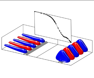
Here, we investigate the three-dimensional structure of the resolvent modes in the low-frequency regime. For this purpose, we plot iso-surfaces of the streamwise (figures 16a,b) and spanwise (figures 16c,d) components of the optimal forcing and response. Iso-surfaces of ${\pm }45\,\%$ of the forcings $|\hat {f}_x|, |\hat {f}_z|$ and the responses $|\hat {u}|, |\hat {w}|$ are displayed, respectively. The time-averaged location of the separation bubble is indicated by the grey-shaded region, which corresponds to the dividing streamline ($\bar {\varPsi }=0$). The frequency is fixed at $St=0.01$, and the non-dimensional spanwise wavenumber is $\beta =1$. In this representation, the distinction between optimal forcing and response is even more prominent. While the optimal forcing is located mostly upstream and in the first half of the TSB (figures 16a,c), the optimal responses $\hat {u}, \hat {w}$ are located in the region surrounding the separation bubble. This particular spatial configuration of forcing and response suggests that upstream disturbances are a required contribution to the low-frequency unsteadiness. Notably, the elongated structures in the upstream region closely resemble boundary layer streaks, albeit with much larger spanwise wavelength compared to usual superstructures in turbulent boundary layers, as discussed in § 2. Whereas the streamwise component of forcing is concentrated in areas parallel to the bottom wall (figure 16a), the structure of the spanwise component is slightly tilted upwards in the TSB region in figure 16(c). This behaviour was also observed for the spanwise forcing at low $\beta$ in Bugeat et al. (Reference Bugeat, Robinet, Chassaing and Sagaut2022), even though the investigated flow was a laminar SBLI.

Figure 16. Streamwise component of (a) optimal forcing $\hat {f}_x$ and (b) response $\hat {u}$, and spanwise component of (c) optimal forcing $\hat {f}_z$ and (d) response $\hat {w}$ from RA, for non-dimensional spanwise wavenumber $\beta =1$. The real parts of the modes are depicted. Iso-surfaces of $\pm 45\,\%$ of $\max |\hat {f}_x|$, $\max |\hat {u}|$ and $\max |\hat {f}_z|$, $\max |\hat {w}|$ are shown, respectively.

In Wu et al. (Reference Wu, Meneveau and Mittal2020), the low-frequency motion of a pressure-induced TSB was related to the presence of a Görtler-type mechanism, which manifests as streamwise-elongated structures in the boundary layer developing over concave walls, or related flows with concave streamlines. Wu et al. (Reference Wu, Meneveau, Mittal, Padovan, Rowley and Cattafesta2022) subsequently investigated the response of the TSB to upstream perturbations via zero-net-mass-flux actuation, and performed a harmonic RA following the method of Padovan, Otto & Rowley (Reference Padovan, Otto and Rowley2020). Their analysis demonstrated that the flow was strongly receptive to streamwise-elongated vortices, which is consistent with our present findings. It is therefore worthwhile investigating if the structures depicted in figure 16 are consistent with a Görtler-type mechanism.

Typically, the characteristic wavelength of Görtler vortices (Görtler Reference Görtler1954) can be expressed as $\lambda _T\approx \delta \unicode{x2013}2 \delta$ (Smits & Dussauge Reference Smits and Dussauge2006), where $\delta$ is the local boundary layer thickness. However, this value was originally introduced for laminar flows, and its applicability to turbulent flows remains ambiguous. Here, we follow the methodology outlined in Wu et al. (Reference Wu, Meneveau and Mittal2020) and compute the characteristic wavelength $\lambda _T$ considering the effective viscosity $\nu _{eff}=\nu +\nu _t$. In the region of mean flow concavity ($x/L_p$ between $-0.1$ and $0.3$), we obtain values $\lambda _T\approx (3\unicode{x2013}7)\delta$. On the other hand, if we convert the characteristic spanwise wavenumber $\beta \approx 1$ that we observe experimentally to a wavelength $\lambda _{LF}$, then we obtain $\lambda _{LF}\approx (11\unicode{x2013}25)\delta$. The observation that $\lambda _{LF}>3\lambda _T$, in conjunction with the absence of any amplified global mode (§ 5.1), indicates that the three-dimensional structures observed in the present flow are probably not related to Görtler vortices.

5.3. Effect of eddy viscosity

Up to this point, all presented results have been computed using the LNSE operator modelling part of the Reynolds stresses by means of an eddy-viscosity model. Here, we briefly discuss the effects of neglecting the eddy viscosity ($\nu _t=0$) on the modal characteristics of the flow as well as the forced dynamics of the bubble. In § 5.1, we identified a stationary weakly damped global mode ($St=0$) that closely resembles the experimentally observed large-scale ‘global’ motion of the TSB when $\beta \approx 1$. Neglecting the $\nu _t$ terms in the LNSE operator of the GMA decreases damping. Whereas the growth rates $\omega _i$ move towards the damping threshold, the frequencies $\omega _r$ are strongly reduced (not shown here). However, no eigenvalue travels into the amplified domain. Further, the so-obtained global modes do not agree well with the experimental findings. As a consequence, the prediction of the modal characteristics of the experimentally observed low-frequency breathing motion appears to be strongly dependent on the incorporation of an eddy-viscosity model.

A similarly strong effect can be observed for the forced dynamics of the bubble. In figure 17, the optimal energy gain $\sigma _1^2$ is displayed for the fixed frequency $St=0.01$, over different non-dimensional spanwise wavenumbers $\beta$. A strongly modified curve can be observed as compared to figure 11, where $\nu _t \neq 0$ (grey-shaded region). The distinct peak observed for $\beta =2.75$ is now barely visible. Only a very slight ‘plateau’ in the expected region of spanwise wavenumbers remains. On the other hand, a maximum for high non-dimensional spanwise wavenumbers becomes apparent at $\beta =40$ ($\lambda _z\approx 0.15 L_b$). This curve looks very similar to the distribution recovered in Bugeat et al. (Reference Bugeat, Robinet, Chassaing and Sagaut2022) in a laminar SBLI; nevertheless, the local maximum at low non-zero $\beta$ is less distinct in the present work. From a physical point of view, the damping of high-wavenumber structures through the inclusion of an eddy-viscosity model, and consequently of small-wavelength structures, is expected. Remarkably, the resolvent modes at $\beta \approx 1$ and low frequency $St\approx 0.01$ (not shown here) look very similar, regardless of whether or not a $\nu _t$ model is employed. The low-frequency selection of structures with $\beta \approx 1$, however, can be uncovered only through the inclusion of the $\nu _t$ model.

Figure 17. Optimal energy gain $\sigma _1^2$ from RA when the terms related to the eddy-viscosity are neglected ($\nu _t=0$) for different non-dimensional spanwise wavenumbers $\beta$ (squares). The frequency is fixed at $St=0.01$. The optimal energy gain, including the eddy-viscosity model in the LNSE operator, is indicated as a grey-shaded region.

6. Discussion

The results presented in § 5 using RA indicate that the TSB base flow amplifies low-frequency ($St \approx 0.01$) and low-wavenumber ($\beta \approx 1$) upstream perturbations. In effect, the flow behaves as a selective amplifier, and the optimal energy gain computed from RA has the form of a first-order low-pass filter with a cut-off frequency of the order of $St \approx 0.01$. In the present section, we review these results and discuss them in light of the experimental database presented in § 2.

We commence by comparing the least damped global mode from the LNSE operator (mode 1) to the optimal response from RA at the fixed frequency $St=0.01$ and the non-dimensional spanwise wavenumber $\beta =1$. Once again, it is crucial to mention that RA exhibits broadly similar low-frequency behaviour when $\beta \le 3$. The streamwise, wall-normal and spanwise components of the respective modes are shown in figures 18(a,b), 18(c,d) and 18(e,f), respectively. The first global mode is shown in figures 18(a,c,e), and the optimal response from RA is shown in figures 18(b,d,f). The optimal response is normalized by the optimal gain $\sigma _1$ to ensure comparability. It is apparent that all components $\hat {u}, \hat {v}, \hat {w}$ share strong similarities, with comparable streamwise and wall-normal extents of the structures, a similar streamwise position $x/L_p$, and a matching phase. In the case of the streamwise modes $\hat {u}$, this equates to a large-scale structure bounding the recirculation region and following its shape, as described in the previous sections. Moreover, the amplitudes of the modes are in good agreement, and the maximum is reached in a similar region of $x/L_p$. Similar trends can be observed for the wall-normal and spanwise modes. Here, the structures are almost a perfect match in terms of position, phase and size. The obvious similarities between the least damped global eigenmode and the resolvent mode strongly suggest that the receptivity at low frequency is occurring from the excitation of the least damped global mode of the TSB (mode 1).

Figure 18. (a,c,e) Global mode 1 and (b,d,f) optimal response from RA for non-dimensional spanwise wavenumber $\beta =1$. The (a,b) streamwise, (c,d) wall-normal and (e,f) spanwise modes are depicted.

We now proceed to investigate the low-frequency unsteadiness observed in the experimental data in more detail. Specifically, our objective is to establish a connection between the low-frequency unsteadiness (breathing) and the described low-frequency receptivity. For this purpose, we first demonstrate that the observed low-frequency dynamics in the experimental data captures a large portion of the total turbulent kinetic energy (TKE) of the flow, that is, that the SPOD spectrum is of ‘low rank’ in the low-frequency regime. Then, we proceed to show analogies between RA and SPOD results.

In figure 19(a), the SPOD eigenvalues $\lambda$ are depicted for all modes and all Strouhal numbers $St$. The eigenvalues are represented as percentages of the total TKE density, ensuring that the summation of all eigenvalues equals $100\,\%$. From figure 19, it becomes apparent that $\lambda _1 \gg \lambda _2$ in the low-frequency region, particularly for $St\approx 0.01$. Therefore, if we investigate the first SPOD mode $\lambda _1$ at the fixed frequency $St=0.01$ (figure 19b), we expect to capture a dominant feature of the flow. Here, the percentage of the TKE of the first mode is approximately $72\,\%$. Further evidence of the low-rank behaviour of both the RA and SPOD operators is provided in figure 20. Here, we plot the ratios between the energy gains $\sigma _1^2/\sigma _2^2$ and between the SPOD eigenvalues $\lambda _1/\lambda _2$. In both cases, in the low-frequency range, the low-rank behaviour is of the order of $10$.

Figure 19. (a) The SPOD eigenvalues $\lambda$ represented as the percentage of all modes. (b) The SPOD eigenvalues $\lambda _i$ at Strouhal number $St=0.01$ represented as percentage of modes at low frequency). The modes $1\unicode{x2013}10$ are depicted, respectively.

Figure 20. Low-rank behaviour of energy gains $\sigma _1^2/\sigma _2^2$ of RA (solid black line and squares) at $\beta =1$, and SPOD eigenvalues $\lambda _1/\lambda _2$ (dashed line) over different Strouhal numbers.

Comparisons between the highest ranking SPOD mode and the optimal response of RA are shown in figures 21(a,c) and 21(b,d), respectively, for $St=0.01$ and $\beta =1$. Here, only the $x/L_p$ region of the PIV measurement plane is depicted. Furthermore, we display the streamwise $\hat {u}$ (figures 21a,b) and wall-normal $\hat {v}$ (figures 21c,d) components, as only those are available from the experiment. In order to address the inherent arbitrariness of the phase in both SPOD and RA, the modes are subjected to a normalization. For this purpose, the phase of $\hat {v}$ is set to zero, while $|\hat {v}|=1$ at the fixed position $x/L_p=0.2$ and $y/\varTheta _0=16$. From figure 21, it becomes apparent that the first SPOD mode and the optimal gain of RA are in close agreement when $St=0.01$ and $\beta =1$. The streamwise component $\hat {u}$ displays a portion of the large structure surrounding the separation bubble as e.g. shown previously in figure 15. The structures are tilted away from the solid bottom wall, and follow the shape of the separated region. Furthermore, an excellent agreement between SPOD and RA can be observed in terms of amplitude and phase. The wall-normal component is also in good agreement with respect to the phase of the structures. A phase shift oriented approximately perpendicular to the shear layer can be observed. The amplitude, however, is slightly larger in the case of the first SPOD mode. The alignment $\varphi$, as introduced in § 4, is $\varphi =0.94$. This large value of $\varphi$ strongly suggests that the low-frequency breathing observed in the experiment is associated with the calculated RA response.

Figure 21. (a,c) Leading SPOD mode of the fluctuating velocity field from experiments and (b,d) optimal response of RA in the region of the PIV measurements. Results at low frequency $St=0.01$ and with $\beta =1$ are depicted. The (a,b) streamwise and (c,d) wall-normal components are displayed. All modes are scaled such that the wall-normal component is $|\hat {v}|=1$ and the phase is zero at a fixed position in space ($x/L_p=0.2$, $y/\varTheta _0=16$).

Interestingly, although the alignment between RA and SPOD is large for $\beta = 1$, the most amplified low-frequency RA mode has spanwise wavenumber $\beta = 2.75$, which is considerably higher than $\beta =1$. Hence, according to RA, structures with $\beta = 2.75$ should be amplified preferably and observed in the experiments instead of the larger $\beta = 1$ structures. A likely explanation for this discrepancy is the finite span of the wind tunnel ($0.6\,{\rm m}$; see § 2), which corresponds approximately to $\beta = 1$, and which might influence the receptivity of the flow by generating strong forcing at this wavenumber. According to this scenario, the experimentally observed $\beta = 1$ structures are preferred over $\beta = 2.75$, although the corresponding gain is approximately 50 % smaller (figure 11). In other words, with a hypothetical wind tunnel of infinite span, it is possible that low-frequency TSB breathing with spanwise wavenumber $\beta \approx 2.75$ would have been observed. While we are not able to substantiate this claim with either experimental or numerical data, we consider this a plausible hypothesis and encourage that further experiments be performed in wider wind tunnels.

We have previously established that any RA mode with $\beta \approx 1$ exhibits the same low-frequency characteristics when $St\approx 0.01$. In figure 22, we display the alignment $\varphi$ between SPOD and RA over the non-dimensional spanwise wavenumber $\beta$ at the fixed frequency $St=0.01$. Both the analysis including an eddy-viscosity model, and the analysis where $\nu _t=0$, are depicted. We obtain two distributions of comparable qualitative nature that feature a maximum for $\beta \approx 1$. However, a strong offset between the alignment for the analysis including an eddy-viscosity model ($\varphi _{max}=0.95$) and the analysis where $\nu _t=0$ ($\varphi _{max}=0.82$) is evident. Clearly, including a $\nu _t$ model into the LNSE operator strongly increases the alignment with the experiment, as represented by the SPOD modes. This is particularly relevant since the overall shape of the resolvent modes is the same whether or not a $\nu _t$ model is included. Interestingly, the significance of implementing an eddy-viscosity model to enhance the alignment between SPOD and RA has been demonstrated in prior studies. For example, Morra et al. (Reference Morra, Semeraro, Henningson and Cossu2019) presented evidence of its relevance in turbulent wall-bounded flows, while Pickering et al. (Reference Pickering, Rigas, Nogueira, Cavalieri, Schmidt and Colonius2020) extended this insight to a turbulent jet configuration.

Figure 22. Alignment $\varphi$ for different non-dimensional spanwise wavenumbers $\beta$. Results with (squares) and without (circles) an eddy-viscosity model are shown.

In summary, the results presented so far demonstrate a strong alignment between the SPOD of the streamwise/wall-normal velocity fluctuations obtained experimentally at low frequency and the optimal RA response computed in the region where $\beta \approx 1$. We further note that both the near-wall velocity and wall-pressure fluctuations in the experiments indicate a characteristic wavenumber of the order of $\beta \approx 1$ for the low-frequency breathing motion (e.g. figure 5). This cements the argument that the unsteadiness observed in the experiment is well described by the RA results. Furthermore, we previously established strong similarities between the least damped LNSE eigenmode and the resolvent response. Hence our conclusion is that the low-frequency breathing motion likely emanates from the excitation of the most weakly damped global mode in the TSB. This phenomenon is not dictated by a singular frequency but rather encompasses a range of low frequencies and low, non-zero spanwise wavenumbers. In effect, the TSB acts like a first-order low-pass filter for upstream disturbances in the incoming turbulent boundary layer.

Interestingly, a low-pass filter model of low-frequency unsteadiness for separation bubbles has already been suggested in different flow configurations. Mohammed-Taifour & Weiss (Reference Mohammed-Taifour and Weiss2021), in a configuration similar to the present one, used pulsed-jet forcing to investigate the response of their TSB to upstream perturbations. They noted that the transient response of the separation line was compatible with a first-order low-pass filter model, and observed consistent low-frequency dynamics in the unforced flow. For the case of turbulent SBLIs, Poggie et al. (Reference Poggie, Bisek, Kimmel and Stanfield2015) investigated the frequency spectra of wall-pressure fluctuations in a variety of test cases, and showed that despite differences in Reynolds and Mach numbers, the first-order model originally proposed by Plotkin (Reference Plotkin1975) and refined by Touber & Sandham (Reference Touber and Sandham2011) for shock-induced separation reasonably collapsed the results. Recently, Bugeat et al. (Reference Bugeat, Robinet, Chassaing and Sagaut2022) proposed a low-pass-filter model for a laminar SBLI, and demonstrated that this behaviour proceeds ‘from the excitation of a single, stable, steady global mode whose damping rate sets the time scale of the filter’. A similar forced modal mechanism was reported in Hao (Reference Hao2023) for a turbulent SBLI. Hence in the case of our TSB, the low-pass filter model is a direct consequence of our proposed mechanism of low-frequency unsteadiness since it is also based on the excitation of a damped global mode. Given the prevalence of low-pass filter behaviour in the literature on separation bubble unsteadiness, these results, combined with those of Bugeat et al. (Reference Bugeat, Robinet, Chassaing and Sagaut2022), suggest that such a mechanism of low-frequency unsteadiness might occur in many types of separation bubbles.

Finally, we briefly come back to our original strategy of performing linear analysis on a DNS base flow that is similar to, but not exactly the same as, the experimental flow field that we consider. In our case, the cross-validation between experimental unsteady data and the DNS base flow was necessary since the DNS did not include any unsteady data at the proper frequency, and the experimental data were not sufficiently resolved spatially to enable a proper linear analysis. Nevertheless, the concordance between the GMA/RA results and the experimental data turned out to be close. This suggests that the phenomenology discovered in this work is not very sensitive to the exact geometry of the flow. Furthermore, the fact that the DNS base flow is devoid of any experimental artefacts, such as inflow unsteadiness, roughness effects, or the presence of wind-tunnel side walls, confirms that the low-frequency breathing motion observed in several low-speed and many high-speed experiments is a relevant fluid dynamical phenomenon that is unlikely to be caused by wind-tunnel effects.

7. Conclusion

The objective of the present work was to perform linear modal and non-modal analysis on an incompressible, pressure-gradient-induced TSB to investigate the origin of the low-frequency breathing motion commonly observed in experimental studies. Specifically, we performed global mode analysis (GMA) and resolvent analysis (RA) on a base flow consisting of the average flow field computed via DNS by Coleman et al. (Reference Coleman, Rumsey and Spalart2018), and we compared the results with the unsteady experimental measurements obtained by Le Floc'h et al. (Reference Le Floc'h, Mohammed-Taifour, Dufresne and Weiss2018, Reference Le Floc'h, Weiss, Mohammed-Taifour and Dufresne2020) in a similar flow field.

The GMA revealed that the eigenmodes of the linearized base flow are damped in the asymptotic time limit for all frequencies and wavenumbers, indicating that the low-frequency unsteadiness is unlikely to be driven by any self-sustained (intrinsic) oscillation. Interestingly, the growth rate $\omega _i$ was closest to the damping threshold in a region of spanwise wavenumbers close to $\beta = 1$. This region was found to agree very well with the range of spanwise wavenumbers extracted from the experimental database at low frequency.

At low frequency and for spanwise wavenumbers lower than $\beta = 3$, RA further revealed an optimal response strongly resembling the unsteady velocity signature of the breathing motion, which typically manifests as a large-scale coherent structure that follows the shape of the bubble. Specifically, a comparison between the first SPOD mode of the streamwise and wall-normal velocity fluctuations measured experimentally showed strong alignment with the optimal RA response, particularly for $\beta \approx 1$. This, combined with the damped eigenmodes of the LNSE operator, indicates that the TSB behaves as an amplifier flow in the low-frequency regime. Furthermore, the optimal gain computed by RA at low non-zero wavenumber was shown to have the characteristic shape of a first-order, low-pass filter with a cut-off frequency consistent with the low-frequency unsteadiness observed experimentally.

Finally, comparison between the least damped global mode and the optimal RA response showed strong similarities in the low-frequency and low-wavenumber regime, and this for all velocity components. This behaviour is considered a strong indication that the low-frequency oscillation is driven primarily by the least damped global mode, thereby characterizing the phenomenon as a forced modal mechanism, associated here with a centrifugal mechanism typical of other separation bubbles (Theofilis et al. Reference Theofilis, Hein and Dallmann2000; Rodríguez et al. Reference Rodríguez, Gennaro and Juniper2013), with the caveat that here we are linearizing the system around the mean flow, and thus the idea of a ‘modal’ mechanism should be taken in a different sense, referring to the properties of the LNSE operator. Hence the main conclusion of this study is that the low-frequency breathing of the TSB is most likely driven by the excitation of a weakly damped global mode by the turbulent fluctuations in the incoming boundary layer. This is consistent with the mechanism proposed recently by Porter & Poggie (Reference Porter and Poggie2019) for the case of turbulent SBLI flows. Our results also bear strong resemblance to the analyses of Bugeat et al. (Reference Bugeat, Robinet, Chassaing and Sagaut2022) and Hao (Reference Hao2023) in a laminar and turbulent SBLI, respectively, thereby suggesting that forced dynamics might be a common feature of separation bubbles in a wide range of flow conditions.

Declaration of interests

The authors report no conflict of interest.

Appendix A. Matrix operators

In this appendix, the matrix operators employed in the GMA and RA are described. We commence by revisiting the equation

(A1)\begin{equation} -{\rm i}\,\omega\boldsymbol{M} \hat{\boldsymbol{q}}=(\boldsymbol{A}+\boldsymbol{N})\hat{\boldsymbol{q}}+\boldsymbol{B}\hat{\boldsymbol{f}}. \end{equation}

The LNSE can be recast into an operator of the form

(A2)\begin{equation} \boldsymbol{A}=\left[\begin{array}{@{}cccc@{}} \xi+\dfrac{\partial \bar{u}}{\partial x}-\dfrac{1}{Re}\,\nabla^2 & \dfrac{\partial \bar{u}}{\partial y} & 0 & \dfrac{\partial}{\partial x} \\ \dfrac{\partial \bar{v}}{\partial x} & \xi+\dfrac{\partial \bar{v}}{\partial y}-\dfrac{1}{Re}\,\nabla^2 & 0 & \dfrac{\partial}{\partial y} \\ 0 & 0 & \xi-\dfrac{1}{Re}\,\nabla^2 & {\rm i}\,\beta \\ \dfrac{\partial}{\partial x} & \dfrac{\partial}{\partial y} & {\rm i}\,\beta & 0 \end{array}\right], \end{equation}

where only the molecular viscosity in the flow is considered. Here, $\xi =(\bar {u}({\partial }/{\partial x})+\bar {v}({\partial }/{\partial y}))$, and $\nabla ^2=({\partial ^2}/{\partial x}+{\partial ^2}/{\partial y}-\beta ^2)$ is the Laplacian.

When the turbulence of the flow is considered by means of an eddy-viscosity model, the additional terms read

(A3)\begin{equation} \boldsymbol{N}=\left[\begin{array}{@{}cccc@{}} -\eta-\dfrac{\partial \nu_{t}}{\partial x}\,\dfrac{\partial}{\partial x} -\nu_{t}\,\nabla^2 & -\dfrac{\partial \nu_{t}}{\partial y}\,\dfrac{\partial}{\partial x} & 0 & 0\\ -\dfrac{\partial \nu_{t}}{\partial x}\,\dfrac{\partial}{\partial y} & -\eta-\dfrac{\partial \nu_{t}}{\partial y}\,\dfrac{\partial }{\partial y}-\nu_{t}\,\nabla^2 & 0 & 0\\ -{\rm i}\,\beta\,\dfrac{\partial \nu_{t}}{\partial x} & -{\rm i}\,\beta\,\dfrac{\partial \nu_{t}}{\partial y} & -\eta-\nu_{t}\,\nabla^2 & 0\\ 0 & 0 & 0 & 0\\ \end{array}\right], \end{equation}

where

(A4)\begin{equation} \eta=\left(\frac{\partial \nu_{t}}{\partial x}\,\frac{\partial}{\partial x}+\frac{\partial \nu_{t}}{\partial y}\,\frac{\partial}{\partial y}\right). \end{equation}

The operator $\boldsymbol {M}$ acts as a mass-like matrix in order to recover the continuity equation

(A5)\begin{equation} \boldsymbol{M}=\left[\begin{array}{@{}cccc@{}} \mathcal{I} & 0 & 0 & 0\\ 0 & \mathcal{I} & 0 & 0\\ 0 & 0 & \mathcal{I} & 0\\ 0 & 0 & 0 & 0 \\ \end{array}\right], \end{equation}

where $\mathcal {I}$ is the identity matrix of respective size. In the resolvent form

(A6)\begin{equation} \hat{\boldsymbol{q}}=\boldsymbol{C}(-{\rm i}\, \omega \boldsymbol{M}-\boldsymbol{A}_{2D,z})^{{-}1}\boldsymbol{B}\hat{\boldsymbol{f}}, \end{equation}

we define the additional matrix operators

(A7a,b)\begin{equation} \boldsymbol{B}=\left[\begin{array}{@{}ccc@{}} b(x) & 0 & 0 \\ 0 & b(x) & 0 \\ 0 & 0 & b(x) \\ 0 & 0 & 0 \\ \end{array}\right], \quad \boldsymbol{C}=\left[\begin{array}{@{}cccc@{}} c(x) & 0 & 0 & 0\\ 0 & c(x) & 0 & 0\\ 0 & 0 & c(x) & 0\\ \end{array}\right]. \end{equation}

The sparse diagonal matrices act as filters that enforce constraints on the forcing and response, respectively. Here, $b(x)=1$ in the region $x\in [0.05L_x, 0.85L_x]$, whereas $b(x)=0$ in the remainder of the domain. Similarly, we set $c(x)=1$ when $x\in [0.33L_x,0.74L_x]$, and $c(x)=0$ elsewhere. Parameter $L_x$ is the length of the domain. The region $x\in [0.33L_x,0.74L_x]$ is chosen to agree with the PIV measurement region, which covers only a portion of the domain of the numerical data.

Appendix B. Boundary conditions and fringe zone

The non-dimensional DNS base flow from Coleman et al. (Reference Coleman, Rumsey and Spalart2018), using the length scale $l^*=L_b$ and the time scale $t^*=L_b/u_\infty$, is depicted in figure 23. In the GMA and RA, we subject the DNS base flow to periodic boundary conditions along the streamwise direction

(B1)\begin{gather} u(x+L_{\rm \pi})=u(x), \end{gather}
(B2)\begin{gather} v(x+L_{\rm \pi})=v(x), \end{gather}

where the periodicity length $L_{\rm \pi}$ is chosen according to $L_{\rm \pi} =0.9N_x$, and $N_x$ is the streamwise dimension of the velocity fields. We further enforce that the disturbances decay at the solid top ($\infty$) and bottom ($0$) walls according to

(B3)\begin{gather} \hat{u}(0)=\hat{v}(0)=\hat{w}(0)=0, \end{gather}
(B4)\begin{gather} \hat{u}(\infty)=\hat{v}(\infty)=\hat{w}(\infty)=0. \end{gather}

Figure 23. Non-dimensional DNS base flow using the length scale $l^*=L_b$ and the time scale $t^*=L_b/u_\infty$. The (a) streamwise $u/u_\infty$ and (b) wall-normal $v/u_\infty$ components of the time-averaged velocity field are displayed.

In order to suppress all disturbances $\hat {u}, \hat {v}, \hat {w}$ as well as forcings $\hat {f}_x, \hat {f}_y, \hat {f}_z$ in the region where the periodic boundary conditions are enforced, a fringe

(B5)\begin{equation} \boldsymbol{S}=\left[\begin{array}{@{}cccc@{}} \sigma_f & 0 & 0 & 0\\ 0 & \sigma_f & 0 & 0\\ 0 & 0 & \sigma_f & 0\\ 0 & 0 & 0 & 0 \\ \end{array}\right] \end{equation}

is added to the two-dimensional LNSE operator $\boldsymbol {A}_{2D,z}=\boldsymbol {A}+\boldsymbol {N}+\boldsymbol {S}$. Here, $\sigma _f$ is a sparse diagonal matrix with $\sigma _f = s_{max}\times \exp (-(x-x_c)^2/L_f^2)$, $s_{max}$ is the maximum amplitude of the fringe, $x_c$ is the centre of the fringe, and $L_f$ is the length. The position and length of the fringe are chosen as $x_c\approx 6L_b$ and $L_f\approx 3.5\,\%\,L_x$, where $L_x$ is the length of the domain.

Appendix C. Grid and fringe convergence

The grid convergence study is presented in figure 24. We portray the first ten singular values of the RA at $\beta =0$. Two Strouhal numbers are displayed: a Strouhal number $St=0.01$, representative of the characteristic low-frequency breathing motion (figure 24a), and a Strouhal number in the medium-frequency regime $St=0.1$ (figure 24b). Four different streamwise ($N_x$) and wall-normal ($N_y$) resolutions are depicted. For a resolution of $N_x \times N_y$ equal to $1200 \times 160$ or higher, a convergence of the results can be observed. Further increasing the grid resolution yields no discernible influence on the singular values of the RA.

Figure 24. Grid convergence study for (a) $St=0.01$ and (b) $St=0.1$ based on RA at $\beta =0$. Grid independence of the singular values of the RA can be observed for $N_x\ge 1200$ and $N_y \ge 160$.

We illustrate the fringe convergence study in figure 25. Once again, we display $St=0.01$ (figure 25a) and $St=0.1$ (figure 25b). We maintain a fixed resolution $N_x=1200$ and $N_y=160$ for the analysis, and test four different magnitudes $s_{max}$. Fringe convergence can then be observed for magnitudes $s_{max}\ge 2$.

Figure 25. Fringe convergence study for (a) $St=0.01$ and (b) $St=0.1$ based on RA at $\beta =0$. Fringe independence of the singular values of the RA can be observed for $s_{max}\ge 2$.

In this work, we perform the GMA and RA analyses with fringe magnitude $s_{max}=5$. All resolvent analyses are performed with resolution $N_x=1200$ and $N_y=160$. A slightly higher resolution, $N_x=1200$ and $N_y=320$, is employed in the case of GMA.

Appendix D. Sub-optimal energy gains

In this appendix, the behaviour of the sub-optimal resolvent modes associated with $\sigma _2, \sigma _3,\ldots, \sigma _n$ and their corresponding forcing fields is studied. Figure 26 shows the sub-optimal energy gains $\sigma _n^2$ at the fixed frequency $St=0.01$, for different non-dimensional spanwise wavenumbers $\beta$. Trends similar to those for the optimal energy gain $\sigma _1^2$ can be observed. The sub-optimal energy gains increase monotonically up to a maximum at low/moderate $\beta$, after which they start to decay. The maximum of the curves, however, is slightly shifted towards higher $\beta$ as compared to figure 11. For instance, $\sigma _2^2$ attains its maximum value for $\beta =4.5$. Furthermore, the low-pass filter behaviour observed in the optimal energy gain $\sigma _1^2$ is not as pronounced for the sub-optimal energy gains. Their behaviour over different Strouhal numbers is shown in figure 27 for the two-dimensional case ($\beta =0$) and the three-dimensional case ($\beta =1$). For three-dimensional perturbations ($\beta =1$), the sub-optimal energy gain $\sigma _2^2$ exhibits a very strong hump at $St=0.06$ and a secondary hump at $St=0.1$ (figure 27b). The low-pass filter behaviour is visible only for $St<0.02$. Similar observations can be made for $\sigma _3^2$. Here, the low-pass filter function is superimposed by a broadband hump centred around $St=0.03$. Only the sub-optimal energy gain $\sigma _4^2$ displays the expected low-pass filter behaviour with a reasonable cut-off frequency.

Figure 26. Sub-optimal energy gain $\sigma _n^2$ from RA for different non-dimensional spanwise wavenumbers $\beta$. The frequency is fixed at $St=0.01$. The displayed sub-optimal gains are $\sigma _2$ (circles), $\sigma _3$ (squares) and $\sigma _4$ (diamonds).

Figure 27. Sub-optimal energy gains $\sigma _n^2$ from RA versus different Strouhal numbers $St$ for (a) the two-dimensional case $\beta =0$, and (b) a sample three-dimensional case $\beta =1$. The displayed sub-optimal energy gains are $\sigma _2^2$ (circles), $\sigma _3^2$ (squares) and $\sigma _4^2$ (diamonds).

Generally speaking, the sub-optimal forcings and responses retain features similar to those of the optimal forcings and responses (figures 13 and 15). However, additional structures away from the bubble and oriented along the base flow shear become apparent; see, for example, figure 28. Combined with the fact that the resolvent operator is low rank at low frequency, as indicated by $\sigma _1^2/\sigma _2^2 \approx 12$, this leads to the inference that the sub-optimal gains are less likely to be responsible for the receptivity at low frequency.

Figure 28. Streamwise component of (a) sub-optimal forcing $\hat {f}_x$ and (b) response $\hat {u}$ related to the sub-optimal energy gain $\sigma _2^2$. The non-dimensional spanwise wavenumber and frequency are $\beta =1$ and $St=0.01$, respectively. The time-averaged location of the TSB is indicated by the dividing streamline $\bar {\varPsi }=0$ (solid black line).

Appendix E. Low non-zero $\beta$ region

In this appendix, we take a closer look at the region $\beta \le 0.25$. In figure 29, we plot the optimal energy gain $\sigma _1^2$ over different Strouhal numbers $St$ for six spanwise wavenumbers $\beta \in [0, 0.25]$. For $\beta =0$, we obtain the same distribution as shown in figure 12(a). The distinct peak at $St\approx 0.1$, which we previously associated with the presence of K–H rollers, remains visible for all $\beta$ shown in figure 29. However, as $\beta$ increases, the optimal energy gain $\sigma _1^2$ in the low-frequency region increases as well. Finally, for $\beta =0.25$, we first observe the expected low-pass filter behaviour, with dominant optimal energy gains in the low-frequency region. The associated contours of optimal forcing and response now appear similar to figure 15 (not shown here). This behaviour can be observed up to approximately $\beta =3$, after which the qualitative shapes of optimal forcing and response start to differ. Taking this into account, we may adopt the (loose) definition of $\beta \in [0.25, 3]$ whenever we refer to the low non-zero $\beta$ region.

Figure 29. Optimal energy gain $\sigma _1^2$ from RA versus different Strouhal numbers $St$ for small spanwise wavenumbers $\beta \le 0.25$. The represented optimal energy gains correspond to $\beta =0$ (dashed line), $\beta =0.05$ (squares), $\beta =0.1$ (circles), $\beta =0.15$ (left-triangles), $\beta =0.2$ (diamonds) and $\beta =0.25$ (triangles).

References

Abe, H. 2017 Reynolds-number dependence of wall-pressure fluctuations in a pressure-induced turbulent separation bubble. J. Fluid Mech. 833, 563598.Google Scholar
Abreu, L.I., Cavalieri, A.V.G., Schlatter, P., Vinuesa, R. & Henningson, D.S. 2020 Spectral proper orthogonal decomposition and resolvent analysis of near-wall coherent structures in turbulent pipe flows. J. Fluid Mech. 900, A11.Google Scholar
Abreu, L.I., Tanarro, A., Cavalieri, A.V.G., Schlatter, P., Vinuesa, R., Hanifi, A. & Henningson, D.S. 2021 Spanwise-coherent hydrodynamic waves around flat plates and airfoils. J. Fluid Mech. 927, A1.Google Scholar
Adler, M.C. & Gaitonde, D.V. 2018 Dynamic linear response of a shock/turbulent-boundary-layer interaction using constrained perturbations. J. Fluid Mech. 840, 291341.Google Scholar
Barkley, D. 2006 Linear analysis of the cylinder wake mean flow. Europhys. Lett. 75 (5), 750756.Google Scholar
Beresh, S.J., Clemens, N.T. & Dolling, D.S. 2002 Relationship between upstream turbulent boundary-layer velocity fluctuations and separation shock unsteadiness. AIAA J. 40 (12), 24122422.Google Scholar
Blanco, D.C.P., Martini, E., Sasaki, K. & Cavalieri, A.V.G. 2022 Improved convergence of the spectral proper orthogonal decomposition through time shifting. J. Fluid Mech. 950, A9.Google Scholar
Bottaro, A., Corbett, P. & Luchini, P. 2003 The effect of base flow variation on flow stability. J. Fluid Mech. 476, 293302.Google Scholar
Boutilier, M.S.H. & Yarusevych, S. 2013 Sensitivity of linear stability analysis of measured separated shear layers. Eur. J. Mech. (B/Fluids) 37, 129142.Google Scholar
Bugeat, B., Robinet, J.-C., Chassaing, J.-C. & Sagaut, P. 2022 Low-frequency resolvent analysis of the laminar oblique shock wave/boundary layer interaction. J. Fluid Mech. 942, A43.Google Scholar
Cavalieri, A.V.G., Jordan, P. & Lesshafft, L. 2019 Wave-packet models for jet dynamics and sound radiation. Appl. Mech. Rev. 71 (2), 020802.Google Scholar
Cherry, N.J., Hillier, R. & Latour, M.E.M.P. 1984 Unsteady measurements in a separated and reattaching flow. J. Fluid Mech. 144, 1346.Google Scholar
Clemens, N.T. & Narayanaswamy, V. 2014 Low-frequency unsteadiness of shock wave/turbulent boundary layer interactions. Annu. Rev. Fluid Mech. 46, 469492.Google Scholar
Coleman, G.N. 2018 DNS: 2-D turbulent separation bubbles. Available at https://turbmodels.larc.nasa.gov/Other_DNS_Data/separation_bubble_2d.html.Google Scholar
Coleman, G.N., Rumsey, C.L. & Spalart, P.R. 2018 Numerical study of turbulent separation bubbles with varying pressure gradient and Reynolds number. J. Fluid Mech. 847, 2870.Google ScholarPubMed
Crow, S.C. & Champagne, F.H. 1971 Orderly structure in jet turbulence. J. Fluid Mech. 48 (3), 547591.Google Scholar
Cura, C., Hanifi, A. & Weiss, J. 2023 Medium-frequency unsteadiness in a turbulent separation bubble. In AIAA SCITECH 2023 Forum, 0095.Google Scholar
Dau, K., Borgmann, D., Little, J.C. & Weiss, J. 2023 Investigation of low frequency unsteadiness in the turbulent separation bubble produced by a wall mounted hump. In AIAA AVIATION 2023 Forum, 4008.Google Scholar
Del Alamo, J.C. & Jimenez, J. 2006 Linear energy amplification in turbulent channels. J. Fluid Mech. 559, 205213.Google Scholar
Dolling, D.S. 2001 Fifty years of shock-wave/boundary-layer interaction research: what next? AIAA J. 39 (8), 15171531.Google Scholar
Dovgal, A.V., Kozlov, V.V. & Michalke, A. 1994 Laminar boundary layer separation: instability and associated phenomena. Prog. Aerosp. Sci. 30 (1), 6194.Google Scholar
Dussauge, J.-P., Dupont, P. & Debiève, J.-F. 2006 Unsteadiness in shock wave boundary layer interactions with separation. Aerosp. Sci. Technol. 10 (2), 8591.Google Scholar
Eaton, J.K. & Johnston, J.P. 1981 A review of research on subsonic turbulent flow reattachment. AIAA J. 19 (9), 10931100.Google Scholar
Ehrenstein, U. & Gallaire, F. 2008 Two-dimensional global low-frequency oscillations in a separating boundary-layer flow. J. Fluid Mech. 614, 315327.Google Scholar
Gaitonde, D.V. 2015 Progress in shock wave/boundary layer interactions. Prog. Aerosp. Sci. 72, 8099.Google Scholar
Ganapathisubramani, B., Clemens, N.T. & Dolling, D.S. 2007 Effects of upstream boundary layer on the unsteadiness of shock-induced separation. J. Fluid Mech. 585, 369394.Google Scholar
Ganapathisubramani, B., Longmire, E.K. & Marusic, I. 2003 Characteristics of vortex packets in turbulent boundary layers. J. Fluid Mech. 478, 3546.Google Scholar
Görtler, H. 1954 On the three-dimensional instability of laminar boundary layers on concave walls. Tech. Memo. 1375. National Advisory Commitee for Aeronautics.Google Scholar
Hao, J. 2023 On the low-frequency unsteadiness in shock wave–turbulent boundary layer interactions. J. Fluid Mech. 971, A28.Google Scholar
Huerre, P. & Monkewitz, P.A. 1990 Local and global instabilities in spatially developing flows. Annu. Rev. Fluid Mech. 22 (1), 473537.Google Scholar
Hutchins, N. & Marusic, I. 2007 Evidence of very long meandering features in the logarithmic region of turbulent boundary layers. J. Fluid Mech. 579, 128.Google Scholar
Hwang, Y. & Cossu, C. 2010 Linear non-normal energy amplification of harmonic and stochastic forcing in the turbulent channel flow. J. Fluid Mech. 664, 5173.Google Scholar
Kiya, M. & Sasaki, K. 1983 Structure of a turbulent separation bubble. J. Fluid Mech. 137, 83113.Google Scholar
Larchevêque, L. 2020 Normalizing low-frequency unsteadiness in compressible separated flows. AIAA 2020-0561. In AIAA SciTech 2020 Forum.Google Scholar
Le Floc'h, A., Mohammed-Taifour, A., Weiss, J., Dufresne, L., Vétel, J. & Jondeau, E. 2016 Effect of boundary-layer superstructures on separation bubble unsteadiness. In 24th International Congress of Theoretical and Applied Mechanics, Montreal, QC, Canada.Google Scholar
Le Floc'h, A., Weiss, J., Mohammed-Taifour, A. & Dufresne, L. 2020 Measurements of pressure and velocity fluctuations in a family of turbulent separation bubbles. J. Fluid Mech. 902, A13.Google Scholar
Le Floc'h, A.S., Mohammed-Taifour, A.T., Dufresne, L. & Weiss, J. 2018 Spanwise aspects of unsteadiness in a pressure-induced turbulent separation bubble. In 2018 Fluid Dynamics Conference, 3538.Google Scholar
Lesshafft, L., Semeraro, O., Jaunet, V., Cavalieri, A.V.G. & Jordan, P. 2019 Resolvent-based modeling of coherent wave packets in a turbulent jet. Phys. Rev. Fluids 4 (6), 063901.Google Scholar
Lumley, J.L. 1970 Stochastic Tools in Turbulence. Academic Press.Google Scholar
Mabey, D.G. 1972 Analysis and correlation of data on pressure fluctuations in separated flow. J. Aircr. 9 (9), 642645.Google Scholar
Marquet, O., Sipp, D., Chomaz, J.-M. & Jacquin, L. 2008 Amplifier and resonator dynamics of a low-Reynolds-number recirculation bubble in a global framework. J. Fluid Mech. 605, 429443.Google Scholar
McKeon, B.J. & Sharma, A.S. 2010 A critical-layer framework for turbulent pipe flow. J. Fluid Mech. 658, 336382.Google Scholar
Michalke, A. 1984 Survey on jet instability theory. Prog. Aerosp. Sci. 21, 159199.Google Scholar
Mohammed-Taifour, A. 2017 Instationnarités dans une bulle de décollement turbulente: étude expérimentale. PhD thesis, École de technologie supérieure.Google Scholar
Mohammed-Taifour, A., Schwaab, Q., Pioton, J. & Weiss, J. 2015 A new wind tunnel for the study of pressure-induced separating and reattaching flows. Aeronaut. J. 119 (1211), 91108.Google Scholar
Mohammed-Taifour, A. & Weiss, J. 2016 Unsteadiness in a large turbulent separation bubble. J. Fluid Mech. 799, 383412.Google Scholar
Mohammed-Taifour, A. & Weiss, J. 2021 Periodic forcing of a large turbulent separation bubble. J. Fluid Mech. 915, A24.Google Scholar
Morra, P., Nogueira, P.A.S., Cavalieri, A.V.G. & Henningson, D.S. 2021 The colour of forcing statistics in resolvent analyses of turbulent channel flows. J. Fluid Mech. 907, A24.Google Scholar
Morra, P., Semeraro, O., Henningson, D.S. & Cossu, C. 2019 On the relevance of Reynolds stresses in resolvent analyses of turbulent wall-bounded flows. J. Fluid Mech. 867, 969984.Google Scholar
Na, Y. & Moin, P. 1998 Direct numerical simulation of a separated turbulent boundary layer. J. Fluid Mech. 374, 379405.Google Scholar
Nichols, J.W., Larsson, J., Bernardini, M. & Pirozzoli, S. 2017 Stability and modal analysis of shock/boundary layer interactions. Theor. Comput. Fluid Dyn. 31, 3350.Google Scholar
Nishioka, M., Asai, M. & Yoshida, S. 1990 Control of flow separation by acoustic excitation. AIAA J. 28 (11), 19091915.Google Scholar
Nogueira, P.A.S., Morra, P., Martini, E., Cavalieri, A.V.G. & Henningson, D.S. 2021 Forcing statistics in resolvent analysis: application in minimal turbulent Couette flow. J. Fluid Mech. 908, A32.Google Scholar
Padovan, A., Otto, S.E. & Rowley, C.W. 2020 Analysis of amplification mechanisms and cross-frequency interactions in nonlinear flows via the harmonic resolvent. J. Fluid Mech. 900, A14.Google Scholar
Pickering, E., Rigas, G., Nogueira, P.A.S., Cavalieri, A.V.G., Schmidt, O.T. & Colonius, T. 2020 Lift-up, Kelvin–Helmholtz and Orr mechanisms in turbulent jets. J. Fluid Mech. 896, A2.Google Scholar
Piponniau, S., Dussauge, J.-P., Debieve, J.-F. & Dupont, P. 2009 A simple model for low-frequency unsteadiness in shock-induced separation. J. Fluid Mech. 629, 87108.Google Scholar
Pirozzoli, S. & Grasso, F. 2006 Direct numerical simulation of impinging shock wave/turbulent boundary layer interaction at $M= 2.25$. Phys. Fluids 18 (6), 065113.Google Scholar
Plotkin, K.J. 1975 Shock wave oscillation driven by turbulent boundary-layer fluctuations. AIAA J. 13 (8), 10361040.Google Scholar
Poggie, J., Bisek, N.J., Kimmel, R.L. & Stanfield, S.A. 2015 Spectral characteristics of separation shock unsteadiness. AIAA J. 53 (1), 200214.Google Scholar
Porter, K.M. & Poggie, J. 2019 Selective upstream influence on the unsteadiness of a separated turbulent compression ramp flow. Phys. Fluids 31 (1), 016104.Google Scholar
Priebe, S., Tu, J.H., Rowley, C.W. & Martín, M.P. 2016 Low-frequency dynamics in a shock-induced separated flow. J. Fluid Mech. 807, 441477.Google Scholar
Rajaee, M., Karlsson, S.K.F. & Sirovich, L. 1994 Low-dimensional description of free-shear-flow coherent structures and their dynamical behaviour. J. Fluid Mech. 258, 129.Google Scholar
Reynolds, W.C. & Hussain, A.K.M.F. 1972 The mechanics of an organized wave in turbulent shear flow. Part 3. Theoretical models and comparisons with experiments. J. Fluid Mech. 54 (2), 263288.Google Scholar
Richardson, R., Zhang, Y., Cattafesta, L.N. & Wu, W. 2023 Low frequency characteristics of a pressure-gradient induced turbulent separation bubble. In AIAA SCITECH 2023 Forum, 0079.Google Scholar
Robinet, J.-C. 2007 Bifurcations in shock-wave/laminar-boundary-layer interaction: global instability approach. J. Fluid Mech. 579, 85112.Google Scholar
Rodríguez, D. & Gennaro, E.M. 2017 Three-dimensional flow stability analysis based on the matrix-forming approach made affordable. In Spectral and High Order Methods for Partial Differential Equations ICOSAHOM 2016: Selected Papers from the ICOSAHOM conference, June 27–July 1, 2016, Rio de Janeiro, Brazil, pp. 639–650. Springer International.Google Scholar
Rodríguez, D., Gennaro, E.M. & Juniper, M.P. 2013 The two classes of primary modal instability in laminar separation bubbles. J. Fluid Mech. 734, R4.Google Scholar
Sansica, A., Sandham, N.D. & Hu, Z. 2016 Instability and low-frequency unsteadiness in a shock-induced laminar separation bubble. J. Fluid Mech. 798, 526.Google Scholar
Sartor, F., Mettot, C., Bur, R. & Sipp, D. 2015 Unsteadiness in transonic shock-wave/boundary-layer interactions: experimental investigation and global stability analysis. J. Fluid Mech. 781, 550577.Google Scholar
Sasaki, K., Barros, D.C., Cavalieri, A.V.G. & Larchevêque, L. 2021 Causality in the shock wave/turbulent boundary layer interaction. Phys. Rev. Fluids 6 (6), 064609.Google Scholar
Schmidt, O.T., Towne, A., Colonius, T., Cavalieri, A.V.G., Jordan, P. & Brès, G.A. 2017 Wavepackets and trapped acoustic modes in a turbulent jet: coherent structure eduction and global stability. J. Fluid Mech. 825, 11531181.Google Scholar
Sipp, D. & Lebedev, A. 2007 Global stability of base and mean flows: a general approach and its applications to cylinder and open cavity flows. J. Fluid Mech. 593, 333358.Google Scholar
Smits, A.J. & Dussauge, J.-P. 2006 Turbulent Shear Layers in Supersonic Flow. Springer Science & Business Media.Google Scholar
Steinfurth, B., Cura, C. & Weiss, J. 2022 Three-dimensional effects associated with the low-frequency breathing motion of a turbulent separation bubble. In 20th International Symposium on Application of Laser and Imaging Techniques to Fluid Mechanics, Lisbon.Google Scholar
Theofilis, V. 2003 Advances in global linear instability analysis of nonparallel and three-dimensional flows. Prog. Aerosp. Sci. 39 (4), 249315.Google Scholar
Theofilis, V. 2011 Global linear instability. Annu. Rev. Fluid Mech. 43, 319352.Google Scholar
Theofilis, V., Hein, S. & Dallmann, U. 2000 On the origins of unsteadiness and three-dimensionality in a laminar separation bubble. Phil. Trans. R. Soc. Lond. A 358 (1777), 32293246.Google Scholar
Tomkins, C.D. & Adrian, R.J. 2003 Spanwise structure and scale growth in turbulent boundary layers. J. Fluid Mech. 490, 3774.Google Scholar
Touber, E. & Sandham, N. 2011 Low-order stochastic modelling of low-frequency motions in reflected shock-wave/boundary-layer interactions. J. Fluid Mech. 671, 417465.Google Scholar
Touber, E. & Sandham, N.D. 2009 Large-eddy simulation of low-frequency unsteadiness in a turbulent shock-induced separation bubble. Theor. Comput. Fluid Dyn. 23, 79107.Google Scholar
Towne, A., Cavalieri, A.V.G., Jordan, P., Colonius, T., Schmidt, O., Jaunet, V. & Brès, G.A. 2017 Acoustic resonance in the potential core of subsonic jets. J. Fluid Mech. 825, 11131152.Google Scholar
Towne, A., Schmidt, O.T. & Colonius, T. 2018 Spectral proper orthogonal decomposition and its relationship to dynamic mode decomposition and resolvent analysis. J. Fluid Mech. 847, 821867.Google Scholar
Wang, S. & Ghaemi, S. 2022 Unsteady motions in the turbulent separation bubble of a two-dimensional wing. J. Fluid Mech. 948, A3.Google Scholar
Weiss, J., Little, J., Threadgill, J. & Gross, A. 2021 Low-frequency unsteadiness in pressure-induced separation bubbles. AIAA 2021-1324. In AIAA SciTech 2021 Forum.Google Scholar
Weiss, J., Mohammed-Taifour, A. & Schwaab, Q. 2015 Unsteady behavior of a pressure-induced turbulent separation bubble. AIAA J. 53 (9), 26342645.Google Scholar
Weiss, J., Steinfurth, B., Chamard, L., Giani, A. & Combette, P. 2022 Spectral proper orthogonal decomposition of unsteady wall shear stress under a turbulent separation bubble. AIAA J. 60 (4), 21502159.Google Scholar
Wu, W., Meneveau, C. & Mittal, R. 2020 Spatio-temporal dynamics of turbulent separation bubbles. J. Fluid Mech. 883, A45.Google Scholar
Wu, W., Meneveau, C., Mittal, R., Padovan, A., Rowley, C.W. & Cattafesta, L. 2022 Response of a turbulent separation bubble to zero-net-mass-flux jet perturbations. Phys. Rev. Fluids 7 (8), 084601.Google Scholar
Yarusevych, S., Sullivan, P.E. & Kawall, J.G. 2006 Coherent structures in an airfoil boundary layer and wake at low Reynolds numbers. Phys. Fluids 18 (4), 044101.Google Scholar
Zare, A., Jovanović, M.R. & Georgiou, T.T. 2017 Colour of turbulence. J. Fluid Mech. 812, 636680.Google Scholar
Figure 0

Figure 1. Schematic of wind tunnel test section with mean streamwise velocity field on the centreline. The time-averaged TSB is indicated by the dividing streamline $\bar {\varPsi }=0$ (solid white line). Here, $H_0$ and $H_1$ indicate the approximate position and width of the near-wall TR-PIV measurements in the ($x\unicode{x2013}z$) plane. Note that the thickness of the indicated PIV planes is representative only and thus not true to scale.

Figure 1

Figure 2. Leading SPOD mode, computed based on planar PIV measurements with $f_{s}=900\,{\rm Hz}$. The (a,c,e,g) streamwise $\hat {u}$ and (b,d,f,h) wall-normal component $\hat {v}$ are shown. The depicted frequencies, from top to bottom, correspond to (a,b) $St=0.01$, (c,d) $St=0.08$, (e,f) $St=0.11$, (g,h) $St=0.27$. The time-averaged location of the TSB is indicated by the dividing streamline $\bar {\varPsi }=0$ (black dashed line).

Figure 2

Figure 3. Frequency–wavenumber spectrum of fluctuating velocity $u'$ in the $x\unicode{x2013}z$ plane at $y\approx 4\,{\rm mm}$ from the test surface. Two streamwise positions $x$ are depicted: (a) a position in the ZPG region upstream of the TSB, $x=1.33\,{\rm m}$, and (b) a position immediately upstream of the time-averaged location of the separation line, $x=1.68\,{\rm m}$. The spanwise wavenumber $\beta =2{\rm \pi} /\lambda _{z}$ is non-dimensionalized by the average bubble length $L_b$. The PSD in the ZPG region (a) is multiplied by a factor of $10$.

Figure 3

Figure 4. (a) The PSD and (b) the pre-multiplied PSD of fluctuation pressure $p'$ for $x_1=1.60\,{\rm m}$ (black) and $x_2=2.05\,{\rm m}$ (blue). The Strouhal number $St$ is calculated based on the bubble length $L_b$ and the reference velocity $U_{ref}=25\,{\rm m}\,{\rm s}^{-1}$.

Figure 4

Figure 5. (a) Spanwise correlation $R_{p^\prime p^\prime }$ of low-pass filtered fluctuating pressure for two streamwise positions, $x_1=1.60\,{\rm m}$ (squares) and $x_2=2.05\,{\rm m}$ (circles) modified from Le Floc'h et al. (2018). (b) Cosine fit $f(z)=c_1 \cos (c_2z)$ of $R_{p^\prime p^\prime }$ (solid line) at $x_1=1.60\,{\rm m}$. The resulting non-dimensional spanwise wavenumber $\beta = (2{\rm \pi} L_{b})/\lambda _{z}$ is equal to $0.97$. The fluctuating pressure at the test-section centreline ($z=0\,{{\rm m}}$) is used as reference for all correlations.

Figure 5

Figure 6. (a) Streamwise velocity component $u/u_\infty$ of experimental flow field. (b) DNS base flow. (c) The pressure distribution along the flat plate is represented by the pressure coefficient $c_p$ for the DNS base flow (solid black line) and the experimental data (circles). The streamwise and wall-normal coordinates are non-dimensionalized by $L_p$ and $\varTheta _0$, respectively. We indicate the time-averaged position of the TSB by means of the dividing streamline (solid white line).

Figure 6

Table 1. Flow characteristics of experimental and numerical database.

Figure 7

Figure 7. Eddy viscosity calculated from DNS data.

Figure 8

Figure 8. Global mode spectra for non-dimensional spanwise wavenumber (a) $\beta =0$ and (b) $\beta =1$. The eigenvalue is $\omega =\omega _i+\omega _r$, where $\omega _i$ is the growth rate, and the Strouhal number is calculated based on $\omega _r$. The least damped stationary (solid red circle) and travelling (dashed blue circle) modes are highlighted for $\beta =1$.

Figure 9

Figure 9. Growth rate $\omega _i$ from GMA over non-dimensional spanwise wavenumber $\beta$. The least damped mode of the spectrum is depicted.

Figure 10

Figure 10. Streamwise component of GMA (a) mode 1 and (b) mode 2 for non-dimensional spanwise wavenumber $\beta =1$. The time-averaged location of the TSB is indicated by the dividing streamline $\bar {\varPsi }=0$ (solid black line).

Figure 11

Figure 11. Optimal energy gain $\sigma _n^2$ from RA for different non-dimensional spanwise wavenumbers $\beta$. The frequency is fixed at $St=0.01$.

Figure 12

Figure 12. Optimal energy gain $\sigma _1^2$ from RA versus different Strouhal numbers $St$ for (a) the two-dimensional case $\beta =0$, and (b) a sample three-dimensional case $\beta =1$.

Figure 13

Figure 13. Streamwise component of (a) optimal forcing $\hat {f}_x$ and (b) response $\hat {u}$ for non-dimensional spanwise wavenumber $\beta =0$ and $St=0.12$. The time-averaged location of the TSB is indicated by the dividing streamline $\bar {\varPsi }=0$ (solid black line).

Figure 14

Figure 14. (a) First-order low-pass filter representation of optimal gain from RA $20\log (\sigma _1)$. (b) Pre-multiplied energy gain $f\, \sigma _1^2$ versus different Strouhal numbers $St$. The non-dimensional spanwise wavenumber is $\beta =1$. The Strouhal number $St_c$ corresponding to the cut-off frequency based on the $-3\,{\rm dB}$ rule is indicated in (a). We further depict the characteristic slope of a first-order low-pass filter $-20\,{\rm dB}\,\text {dec}^{-1}$ (dashed red line).

Figure 15

Figure 15. Streamwise component of (a) optimal forcing $\hat {f}_x$ and (b) response $\hat {u}$ for non-dimensional spanwise wavenumber $\beta =1$ and $St=0.01$. The time-averaged location of the TSB is indicated by the dividing streamline $\bar {\varPsi }=0$ (solid black line).

Figure 16

Figure 16. Streamwise component of (a) optimal forcing $\hat {f}_x$ and (b) response $\hat {u}$, and spanwise component of (c) optimal forcing $\hat {f}_z$ and (d) response $\hat {w}$ from RA, for non-dimensional spanwise wavenumber $\beta =1$. The real parts of the modes are depicted. Iso-surfaces of $\pm 45\,\%$ of $\max |\hat {f}_x|$, $\max |\hat {u}|$ and $\max |\hat {f}_z|$, $\max |\hat {w}|$ are shown, respectively.

Figure 17

Figure 17. Optimal energy gain $\sigma _1^2$ from RA when the terms related to the eddy-viscosity are neglected ($\nu _t=0$) for different non-dimensional spanwise wavenumbers $\beta$ (squares). The frequency is fixed at $St=0.01$. The optimal energy gain, including the eddy-viscosity model in the LNSE operator, is indicated as a grey-shaded region.

Figure 18

Figure 18. (a,c,e) Global mode 1 and (b,d,f) optimal response from RA for non-dimensional spanwise wavenumber $\beta =1$. The (a,b) streamwise, (c,d) wall-normal and (e,f) spanwise modes are depicted.

Figure 19

Figure 19. (a) The SPOD eigenvalues $\lambda$ represented as the percentage of all modes. (b) The SPOD eigenvalues $\lambda _i$ at Strouhal number $St=0.01$ represented as percentage of modes at low frequency). The modes $1\unicode{x2013}10$ are depicted, respectively.

Figure 20

Figure 20. Low-rank behaviour of energy gains $\sigma _1^2/\sigma _2^2$ of RA (solid black line and squares) at $\beta =1$, and SPOD eigenvalues $\lambda _1/\lambda _2$ (dashed line) over different Strouhal numbers.

Figure 21

Figure 21. (a,c) Leading SPOD mode of the fluctuating velocity field from experiments and (b,d) optimal response of RA in the region of the PIV measurements. Results at low frequency $St=0.01$ and with $\beta =1$ are depicted. The (a,b) streamwise and (c,d) wall-normal components are displayed. All modes are scaled such that the wall-normal component is $|\hat {v}|=1$ and the phase is zero at a fixed position in space ($x/L_p=0.2$, $y/\varTheta _0=16$).

Figure 22

Figure 22. Alignment $\varphi$ for different non-dimensional spanwise wavenumbers $\beta$. Results with (squares) and without (circles) an eddy-viscosity model are shown.

Figure 23

Figure 23. Non-dimensional DNS base flow using the length scale $l^*=L_b$ and the time scale $t^*=L_b/u_\infty$. The (a) streamwise $u/u_\infty$ and (b) wall-normal $v/u_\infty$ components of the time-averaged velocity field are displayed.

Figure 24

Figure 24. Grid convergence study for (a) $St=0.01$ and (b) $St=0.1$ based on RA at $\beta =0$. Grid independence of the singular values of the RA can be observed for $N_x\ge 1200$ and $N_y \ge 160$.

Figure 25

Figure 25. Fringe convergence study for (a) $St=0.01$ and (b) $St=0.1$ based on RA at $\beta =0$. Fringe independence of the singular values of the RA can be observed for $s_{max}\ge 2$.

Figure 26

Figure 26. Sub-optimal energy gain $\sigma _n^2$ from RA for different non-dimensional spanwise wavenumbers $\beta$. The frequency is fixed at $St=0.01$. The displayed sub-optimal gains are $\sigma _2$ (circles), $\sigma _3$ (squares) and $\sigma _4$ (diamonds).

Figure 27

Figure 27. Sub-optimal energy gains $\sigma _n^2$ from RA versus different Strouhal numbers $St$ for (a) the two-dimensional case $\beta =0$, and (b) a sample three-dimensional case $\beta =1$. The displayed sub-optimal energy gains are $\sigma _2^2$ (circles), $\sigma _3^2$ (squares) and $\sigma _4^2$ (diamonds).

Figure 28

Figure 28. Streamwise component of (a) sub-optimal forcing $\hat {f}_x$ and (b) response $\hat {u}$ related to the sub-optimal energy gain $\sigma _2^2$. The non-dimensional spanwise wavenumber and frequency are $\beta =1$ and $St=0.01$, respectively. The time-averaged location of the TSB is indicated by the dividing streamline $\bar {\varPsi }=0$ (solid black line).

Figure 29

Figure 29. Optimal energy gain $\sigma _1^2$ from RA versus different Strouhal numbers $St$ for small spanwise wavenumbers $\beta \le 0.25$. The represented optimal energy gains correspond to $\beta =0$ (dashed line), $\beta =0.05$ (squares), $\beta =0.1$ (circles), $\beta =0.15$ (left-triangles), $\beta =0.2$ (diamonds) and $\beta =0.25$ (triangles).