


1. Introduction
Short ocean surface waves are hydrodynamically modulated by longer swell. As long waves propagate through a field of shorter waves, their orbital velocities cause near-surface convergence and divergence on the front and rear faces of the long waves, respectively. Following Unna (Reference Unna1941, Reference Unna1942, Reference Unna1947), Longuet-Higgins & Stewart (Reference Longuet-Higgins and Stewart1960) introduced a steady, approximate solution for hydrodynamic modulation of short waves by longer waves
 \begin{equation} \widetilde {k} = k (1 + \varepsilon _L \cos {\psi }), \end{equation}
where $\widetilde {k}$
and
$\widetilde {k}$
and $k$
are the modulated and unmodulated short-wave wavenumbers, respectively,
$k$
are the modulated and unmodulated short-wave wavenumbers, respectively, $\varepsilon _L = a_L k_L$
is the steepness of the long wave with wavenumber
$\varepsilon _L = a_L k_L$
is the steepness of the long wave with wavenumber $k_L$
and amplitude
$k_L$
and amplitude $a_L$
and
$a_L$
and $\psi$
is the long-wave phase. This process is illustrated in figure 1. Hydrodynamic modulation is a key process for the development and interpretation of remote sensing of ocean surface waves and currents (Keller & Wright Reference Keller and Wright1975; Alpers & Hasselmann Reference Alpers and Hasselmann1978; Hara & Plant Reference Hara and Plant1994) and is distinguished from aerodynamic modulation (Donelan Reference Donelan1987; Belcher Reference Belcher1999; Chen & Belcher Reference Chen and Belcher2000). Experimental studies of the general short-wave modulation problem included both the laboratory (e.g. Keller & Wright Reference Keller and Wright1975; Donelan et al. Reference Donelan, Haus, Plant and Troianowski2010 and field (e.g. Plant Reference Plant1977; Hara et al. Reference Hara, Hanson, Bock and Uz2003) measurements. Phillips (Reference Phillips1981) and Longuet-Higgins (Reference Longuet-Higgins1987) revisited the hydrodynamic modulation problem by considering nonlinear long waves and variations in the effective gravity of short waves. Their results yielded significantly stronger modulation than previously predicted by Longuet-Higgins & Stewart (Reference Longuet-Higgins and Stewart1960). Henyey et al. (Reference Henyey, Creamer, Dysthe, Schult and Wright1988) derived an analytical solution for the modulation of short waves using Hamiltonian mechanics and reported similar modulation magnitudes to that of Longuet-Higgins (Reference Longuet-Higgins1987). Zhang & Melville (Reference Zhang and Melville1990) considered weakly nonlinear short waves using a nonlinear Schrödinger equation and found stronger wavenumber modulation but weaker amplitude modulation than those predicted by Longuet-Higgins (Reference Longuet-Higgins1987). Aside from the early linear solutions by Longuet-Higgins & Stewart (Reference Longuet-Higgins and Stewart1960), the variety of analytical and numerical frameworks (Eulerian crest and action conservation, Hamiltonian, Schrödinger) that tackle the same fundamental physics and that relatively closely reproduce the steady solutions for short-wave modulation suggests that the solutions are robust. Nevertheless, alternative analytical and numerical approaches to the modulation problem remain of interest, especially if higher degrees of nonlinearity can be considered using simpler approaches.
$\psi$
is the long-wave phase. This process is illustrated in figure 1. Hydrodynamic modulation is a key process for the development and interpretation of remote sensing of ocean surface waves and currents (Keller & Wright Reference Keller and Wright1975; Alpers & Hasselmann Reference Alpers and Hasselmann1978; Hara & Plant Reference Hara and Plant1994) and is distinguished from aerodynamic modulation (Donelan Reference Donelan1987; Belcher Reference Belcher1999; Chen & Belcher Reference Chen and Belcher2000). Experimental studies of the general short-wave modulation problem included both the laboratory (e.g. Keller & Wright Reference Keller and Wright1975; Donelan et al. Reference Donelan, Haus, Plant and Troianowski2010 and field (e.g. Plant Reference Plant1977; Hara et al. Reference Hara, Hanson, Bock and Uz2003) measurements. Phillips (Reference Phillips1981) and Longuet-Higgins (Reference Longuet-Higgins1987) revisited the hydrodynamic modulation problem by considering nonlinear long waves and variations in the effective gravity of short waves. Their results yielded significantly stronger modulation than previously predicted by Longuet-Higgins & Stewart (Reference Longuet-Higgins and Stewart1960). Henyey et al. (Reference Henyey, Creamer, Dysthe, Schult and Wright1988) derived an analytical solution for the modulation of short waves using Hamiltonian mechanics and reported similar modulation magnitudes to that of Longuet-Higgins (Reference Longuet-Higgins1987). Zhang & Melville (Reference Zhang and Melville1990) considered weakly nonlinear short waves using a nonlinear Schrödinger equation and found stronger wavenumber modulation but weaker amplitude modulation than those predicted by Longuet-Higgins (Reference Longuet-Higgins1987). Aside from the early linear solutions by Longuet-Higgins & Stewart (Reference Longuet-Higgins and Stewart1960), the variety of analytical and numerical frameworks (Eulerian crest and action conservation, Hamiltonian, Schrödinger) that tackle the same fundamental physics and that relatively closely reproduce the steady solutions for short-wave modulation suggests that the solutions are robust. Nevertheless, alternative analytical and numerical approaches to the modulation problem remain of interest, especially if higher degrees of nonlinearity can be considered using simpler approaches.
Figure 1. A diagram of short waves riding on longer waves that propagate with their phase speed $C_{pL}$
from left to right. The short waves propagate on the long-wave surface, their action moving with the group velocity
$C_{pL}$
from left to right. The short waves propagate on the long-wave surface, their action moving with the group velocity $C_g$
. Long waves induce horizontal and vertical orbital velocities
$C_g$
. Long waves induce horizontal and vertical orbital velocities $U$
and W, respectively, that cause near-surface convergence and divergence on their front and rear faces, respectively. They also induce downward and upward centripetal accelerations (
$U$
and W, respectively, that cause near-surface convergence and divergence on their front and rear faces, respectively. They also induce downward and upward centripetal accelerations ( ${\textrm d}W/{\textrm d}t$
) in the crests and troughs, respectively, that modulate the effective gravity at the surface. As a consequence of surface convergence and divergence and the effective-gravity modulation, the short waves become shorter and higher preferentially on the long-wave crests. The diagram is not to scale.
${\textrm d}W/{\textrm d}t$
) in the crests and troughs, respectively, that modulate the effective gravity at the surface. As a consequence of surface convergence and divergence and the effective-gravity modulation, the short waves become shorter and higher preferentially on the long-wave crests. The diagram is not to scale.
All modulation solutions mentioned thus far are steady in the reference frame of the long wave – short waves become shorter and higher (and thus, steeper) preferentially on the long-wave crests. Conversely, they elongate and flatten preferentially in the long-wave troughs. Recently, Peureux, Ardhuin & Guimarães (Reference Peureux, Ardhuin and Guimarães2021) asked whether the steady (i.e. stationary; not depending on time) solutions of short-wave modulation are appropriate by simulating the full wave conservation equations. They found that the short waves grow unsteadily due to the propagation of longer waves, suggesting that the steady-state solutions may only be valid for a few long-wave periods before the short waves begin to break due to excessive steepness. However, the unsteadiness of their solutions occurs in a specific scenario in which a long-wave train suddenly appears to modulate a uniform field of short waves. The numerical simulations stabilise if the short-wave field is initialised from existing steady solutions, like those by Longuet-Higgins & Stewart (Reference Longuet-Higgins and Stewart1960). Nevertheless, their results do put into question whether the short-wave modulation predicted by theory is generally steady over many long-wave periods or not. Looking at the conservation equations alone, it is not obvious that it is.
In this paper, we revisit this problem from the perspective of wave action conservation but consider the long-wave slope to be significant enough to require evaluating the short waves at the long-wave surface rather than at the mean water level. This allows us to derive alternative, steady, nonlinear solutions for the modulation of short waves, within the limits of small $\varepsilon _L$
. The analytical solutions yield modulations that are stronger than the original solution by Longuet-Higgins & Stewart (Reference Longuet-Higgins and Stewart1960), but similar to the nonlinear numerical solutions by Longuet-Higgins (Reference Longuet-Higgins1987) and Zhang & Melville (Reference Zhang and Melville1990) for
$\varepsilon _L$
. The analytical solutions yield modulations that are stronger than the original solution by Longuet-Higgins & Stewart (Reference Longuet-Higgins and Stewart1960), but similar to the nonlinear numerical solutions by Longuet-Higgins (Reference Longuet-Higgins1987) and Zhang & Melville (Reference Zhang and Melville1990) for $\varepsilon _L \lesssim 0.2$
. To validate the steadiness of the analytical solutions, we perform numerical simulations of the full wave crest and action conservation laws, and compare the results with the analytical solutions presented here, as well as the prior numerical results. The numerical simulations are used to determine the validity of the approximate steady solution and to investigate the unsteadiness of the short-wave modulation found by Peureux et al. (Reference Peureux, Ardhuin and Guimarães2021). The main prior studies on hydrodynamic modulation, and their assumptions and approaches to the solution, are summarised in table 1. We first present the governing equations in § 2, and then the analytical solutions for the modulation of short waves by long waves in § 3. Then, we describe the numerical simulations and their results in § 4. Finally, we discuss the results and their implications in § 5 and conclude the paper in § 6.
$\varepsilon _L \lesssim 0.2$
. To validate the steadiness of the analytical solutions, we perform numerical simulations of the full wave crest and action conservation laws, and compare the results with the analytical solutions presented here, as well as the prior numerical results. The numerical simulations are used to determine the validity of the approximate steady solution and to investigate the unsteadiness of the short-wave modulation found by Peureux et al. (Reference Peureux, Ardhuin and Guimarães2021). The main prior studies on hydrodynamic modulation, and their assumptions and approaches to the solution, are summarised in table 1. We first present the governing equations in § 2, and then the analytical solutions for the modulation of short waves by long waves in § 3. Then, we describe the numerical simulations and their results in § 4. Finally, we discuss the results and their implications in § 5 and conclude the paper in § 6.
Table 1. Non-exhaustive summary of prior and present (this paper) approaches to calculating the modulation of short waves by long waves. The solution steadiness refers to whether the solution depends on time (unsteady) or not (steady).
2. Governing equations
The flow is inviscid, irrotational and incompressible, and without sources or sinks. In these conditions, linear, deep-water, surface gravity waves obey the dispersion relation
 \begin{equation} \omega = \sqrt {gk} + k U, \end{equation}
where $\omega$
is the angular frequency in a fixed reference frame,
$\omega$
is the angular frequency in a fixed reference frame, $g$
is the gravitational acceleration,
$g$
is the gravitational acceleration, $k$
is the wavenumber and
$k$
is the wavenumber and $U$
is the mean advective current in the direction of the wave propagation. A current in the direction of the waves increases their absolute frequency without changing their wavenumber. An important limitation here is that
$U$
is the mean advective current in the direction of the wave propagation. A current in the direction of the waves increases their absolute frequency without changing their wavenumber. An important limitation here is that $U$
must be slowly varying on the scales of the wave period (Bretherton & Garrett Reference Bretherton and Garrett1968). From the perspective of short waves riding on long waves, the advective current is the horizontal near-surface orbital velocity of the long wave. Strictly, shear must be considered when determining the advective velocity for a wave of any given wavenumber (Stewart & Joy Reference Stewart and Joy1974; Ellingsen Reference Ellingsen2014). Here, we assume the surface velocity to be the advective one for short waves, and demonstrate later in
$U$
must be slowly varying on the scales of the wave period (Bretherton & Garrett Reference Bretherton and Garrett1968). From the perspective of short waves riding on long waves, the advective current is the horizontal near-surface orbital velocity of the long wave. Strictly, shear must be considered when determining the advective velocity for a wave of any given wavenumber (Stewart & Joy Reference Stewart and Joy1974; Ellingsen Reference Ellingsen2014). Here, we assume the surface velocity to be the advective one for short waves, and demonstrate later in $\S$
3.4 that this is valid for sufficient scale separation between the short and long waves. The evolution of the short-wave wavenumber is described by the conservation of wave crests (e.g. Whitham Reference Whitham1974; Phillips Reference Phillips1981)
$\S$
3.4 that this is valid for sufficient scale separation between the short and long waves. The evolution of the short-wave wavenumber is described by the conservation of wave crests (e.g. Whitham Reference Whitham1974; Phillips Reference Phillips1981)
 \begin{equation} \dfrac {\partial k}{\partial t} + \dfrac {\partial \omega }{\partial x} = 0, \end{equation}
where $t$
and
$t$
and $x$
are time and space, respectively. This relation states that the wavenumber must change locally when the frequency varies in space.
$x$
are time and space, respectively. This relation states that the wavenumber must change locally when the frequency varies in space.
Equations (2.1) and (2.2) describe the evolution of the short-wave wavenumber. To describe the evolution of the wave amplitude, we use the wave action balance (Bretherton & Garrett Reference Bretherton and Garrett1968) in the absence of sources (e.g. due to wind) and sinks (e.g. due to whitecapping)
 \begin{equation} \dfrac {\partial N}{\partial t} + \dfrac {\partial }{\partial x} \left [\left (C_g + U\right )N\right ] = 0, \end{equation}
where $N$
is the action of short waves defined as the ratio of their energy to their intrinsic frequency,
$N$
is the action of short waves defined as the ratio of their energy to their intrinsic frequency, $E/\sigma$
, and
$E/\sigma$
, and $C_g = 1/2\sqrt {g/k}$
is their group speed in deep water. The wave action expressed as
$C_g = 1/2\sqrt {g/k}$
is their group speed in deep water. The wave action expressed as $E/\sigma$
is commonly taken as conservative in wave modulation theory (Phillips Reference Phillips1981; Longuet-Higgins Reference Longuet-Higgins1987), however, as Dysthe et al. (Reference Dysthe, Henyey, Longuet-Higgins and Schult1988) show, it is conservative only for gently sloped waves. We describe this and other requirements in more detail further below and show in what long-wave conditions they are satisfied. The wave crest conservation (2.2) follows from the assumption of a conserved wave phase, and is another prerequisite for wave action conservation (e.g. Whitham Reference Whitham1974). Although the absence of wave growth and dissipation is not generally realistic in the open ocean, it is a useful approximation here to isolate the effects of hydrodynamic modulation solely due to the motion of the long waves. The governing equations (2.1)–(2.3) are derived in Appendix A.
$E/\sigma$
is commonly taken as conservative in wave modulation theory (Phillips Reference Phillips1981; Longuet-Higgins Reference Longuet-Higgins1987), however, as Dysthe et al. (Reference Dysthe, Henyey, Longuet-Higgins and Schult1988) show, it is conservative only for gently sloped waves. We describe this and other requirements in more detail further below and show in what long-wave conditions they are satisfied. The wave crest conservation (2.2) follows from the assumption of a conserved wave phase, and is another prerequisite for wave action conservation (e.g. Whitham Reference Whitham1974). Although the absence of wave growth and dissipation is not generally realistic in the open ocean, it is a useful approximation here to isolate the effects of hydrodynamic modulation solely due to the motion of the long waves. The governing equations (2.1)–(2.3) are derived in Appendix A.
Short waves that ride on the surface of the longer waves move in an accelerated reference frame (due to the centripetal acceleration at the long-wave surface) and thus experience effective gravitational acceleration that varies in space and time (Phillips Reference Phillips1981; Longuet-Higgins Reference Longuet-Higgins1986, Reference Longuet-Higgins1987). Inserting (2.1) into (2.2) and noting that
 \begin{equation} \dfrac {\partial \sqrt {gk}}{\partial x} = \dfrac {1}{2} \sqrt {\dfrac {g}{k}} \dfrac {\partial k}{\partial x} + \dfrac {1}{2} \sqrt {\dfrac {k}{g}} \dfrac {\partial g}{\partial x}, \end{equation}
we get
 \begin{equation} \dfrac {\partial k}{\partial t} + \left (C_g + U\right ) \dfrac {\partial k}{\partial x} + k \dfrac {\partial U}{\partial x} + \dfrac {1}{2} \sqrt {\dfrac {k}{g}} \dfrac {\partial g}{\partial x} = 0. \end{equation}
From left to right, the terms in this equation represent the change in wavenumber due to the propagation and advection by ambient current $U$
, the convergence of the ambient current and the spatial inhomogeneity of the gravitational acceleration. In a non-accelerated reference frame (i.e. in the absence of longer waves), the last term vanishes. It is otherwise necessary to conserve the wave crests.
$U$
, the convergence of the ambient current and the spatial inhomogeneity of the gravitational acceleration. In a non-accelerated reference frame (i.e. in the absence of longer waves), the last term vanishes. It is otherwise necessary to conserve the wave crests.
For the wave action, we expand (2.3) to get
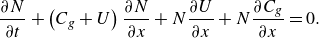 \begin{equation} \dfrac {\partial N}{\partial t} + \left (C_g + U\right ) \dfrac {\partial N}{\partial x} + N \dfrac {\partial U}{\partial x} + N \dfrac {\partial C_g}{\partial x} = 0. \end{equation}
This equation is similar to (2.5), except for the last term, which represents the inhomogeneity of the group speed. As Peureux et al. (Reference Peureux, Ardhuin and Guimarães2021) explained, the presence of this term causes unsteady growth of wave action in infinite long-wave trains. Equations (2.5) and (2.6) are the governing equations that we approximate and solve analytically in § 3, and numerically in their full form in § 4. This system of equations is semi-coupled, meaning that it is possible to solve (2.5) on its own, but solving (2.6) requires also the solution of (2.5). In other words, the wave kinematics (the wavenumber distribution) are not concerned with the wave action. In contrast, the wave action is governed, among others, by the group velocity and thus depends on the wavenumber. This convenient property is only possible if we consider the linear form of the dispersion relation, that is, if the series are truncated at the second-order solution in the Stokes expansion. For a third-order expansion, an additional term that is proportional to the square of the wave steepness appears in the dispersion relation. In that case, (2.5) and (2.6) become fully coupled and the analytical solution for the wavenumber is no longer feasible.
For the ambient forcing, we consider a train of monochromatic long waves defined, to the first order in $\varepsilon _L$
, by the elevation
$\varepsilon _L$
, by the elevation $\eta _L = a_L \cos {\psi }$
, where
$\eta _L = a_L \cos {\psi }$
, where $\psi = k_L x - \sigma _L t$
is the long-wave phase and
$\psi = k_L x - \sigma _L t$
is the long-wave phase and $\sigma _L$
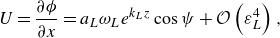
its angular frequency. The velocity potential of the long wave is
$\sigma _L$
its angular frequency. The velocity potential of the long wave is
 \begin{equation} \phi = \dfrac {a_L \omega _L}{k_L} e^{k_L z} \sin {\psi } + {\mathcal{O}}\left(\varepsilon _L^4\right), \end{equation}
where $z$
is the vertical distance from the mean water level that is positive upwards. When evaluated at the mean water level (
$z$
is the vertical distance from the mean water level that is positive upwards. When evaluated at the mean water level ( $z=0$
), (2.7) is accurate to the third order in
$z=0$
), (2.7) is accurate to the third order in $\varepsilon _L$
in deep water because the second- and third-order terms in the Stokes expansion series are exactly zero. The long-wave induced horizontal and vertical orbital velocities are
$\varepsilon _L$
in deep water because the second- and third-order terms in the Stokes expansion series are exactly zero. The long-wave induced horizontal and vertical orbital velocities are
 \begin{equation} U = \frac {\partial \phi }{\partial x} = a_L \omega _L e^{k_L z} \cos {\psi } + {\mathcal{O}}\left(\varepsilon _L^4\right), \end{equation}
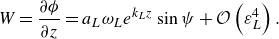 \begin{equation} W = \frac {\partial \phi }{\partial z} = a_L \omega _L e^{k_L z} \sin {\psi } + {\mathcal{O}}\left(\varepsilon _L^4\right). \end{equation}
Evaluating these velocities at the wave surface $z = \eta _L$
rather than at the mean water level
$z = \eta _L$
rather than at the mean water level $z=0$
is a departure from the linear theory, making the treatment of the long waves here weakly nonlinear. As Zhang & Melville (Reference Zhang and Melville1990) point out, this is appropriate to do when the amplitude of the long waves is of similar magnitude to or larger than the wavelength of the short waves. However, evaluating these velocities at the free surface
$z=0$
is a departure from the linear theory, making the treatment of the long waves here weakly nonlinear. As Zhang & Melville (Reference Zhang and Melville1990) point out, this is appropriate to do when the amplitude of the long waves is of similar magnitude to or larger than the wavelength of the short waves. However, evaluating these velocities at the free surface $z = \eta _L$
introduces an additional error of
$z = \eta _L$
introduces an additional error of ${\mathcal{O}}(\varepsilon _L^2)$
. The surface velocity errors are described in more detail in Appendix B.
${\mathcal{O}}(\varepsilon _L^2)$
. The surface velocity errors are described in more detail in Appendix B.
Equations (2.5)–(2.6) are the governing equations used in this paper, with (2.8)–(2.9) describing the long-wave induced ambient velocity forcing for the short waves. Rather than deriving the modulation solution from the velocity potential of two waves, as Longuet-Higgins & Stewart (Reference Longuet-Higgins and Stewart1960) did, starting from the crest-action conservation balances allows for a simpler derivation.
3. Analytical solutions
We now describe the analytical solutions for the short-wave wavenumber, effective gravitational acceleration, amplitude and steepness in the presence of long waves. The wavenumber is derived by linearising the conservation of wave crests (2.2) and neglecting the spatial gradients of $k$
and
$k$
and $g$
. The effective gravity is derived by projecting the long-wave induced surface accelerations onto the local vertical axis (that is, the axis normal to the long-wave surface), akin to Zhang & Melville (Reference Zhang and Melville1990). The amplitude is derived by first evaluating the short-wave action from the action conservation (2.3) and then applying the modulated effective gravity to obtain the amplitude. From the modulated wavenumber, amplitude and effective gravity, the steepness, frequency and phase speed readily follow from the usual wave relationships. Going forward we will use the tilde over the variables to denote the modulated quantities (e.g.
$g$
. The effective gravity is derived by projecting the long-wave induced surface accelerations onto the local vertical axis (that is, the axis normal to the long-wave surface), akin to Zhang & Melville (Reference Zhang and Melville1990). The amplitude is derived by first evaluating the short-wave action from the action conservation (2.3) and then applying the modulated effective gravity to obtain the amplitude. From the modulated wavenumber, amplitude and effective gravity, the steepness, frequency and phase speed readily follow from the usual wave relationships. Going forward we will use the tilde over the variables to denote the modulated quantities (e.g. $\widetilde{k}$
for wavenumber).
$\widetilde{k}$
for wavenumber).
3.1. Wavenumber modulation
Solving analytically for the wavenumber requires dropping the spatial derivatives of $k$
in (2.5) and assuming homogeneous
$k$
in (2.5) and assuming homogeneous $g$
$g$
 \begin{equation} \dfrac {\partial k}{\partial t} = - k \dfrac {\partial U}{\partial x}. \end{equation}
Although Peureux et al. (Reference Peureux, Ardhuin and Guimarães2021) pointed out that the solution by Longuet-Higgins & Stewart (Reference Longuet-Higgins and Stewart1960) requires assuming homogeneous group speed of the short-wave field, in fact, it also requires assuming no horizontal propagation and advection of the short waves. We combine (2.8) and (3.1) and integrate in time to get
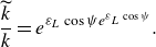 \begin{equation} \frac {\widetilde {k}}{k} = e^{\varepsilon _L \cos {\psi } e^{\varepsilon _L \cos {\psi }}}. \end{equation}
Notice that the Taylor expansion of (3.2) to the first order recovers the original solution by Longuet-Higgins & Stewart (Reference Longuet-Higgins and Stewart1960)
 \begin{equation} \frac {\widetilde {k}}{k} = 1 + \varepsilon _L \cos {\psi }. \end{equation}
Coming from the conservation of crests, as opposed to the velocity potential superposition, the solution by Longuet-Higgins & Stewart (Reference Longuet-Higgins and Stewart1960) requires two approximations: first, evaluating the long-wave velocity at $z = 0$
rather than
$z = 0$
rather than $z = \eta _L$
; and second, truncating the Taylor expansion series beyond
$z = \eta _L$
; and second, truncating the Taylor expansion series beyond ${\mathcal{O}}(\varepsilon _L)$
. These approximations underestimate the short-wave modulation magnitude (figure. 2). At the wave crest, (3.2) yields the wavenumber modulation that is 16.9 %, 38.5 %, 66.4 % and 104 % larger than that of Longuet-Higgins & Stewart (Reference Longuet-Higgins and Stewart1960) for
${\mathcal{O}}(\varepsilon _L)$
. These approximations underestimate the short-wave modulation magnitude (figure. 2). At the wave crest, (3.2) yields the wavenumber modulation that is 16.9 %, 38.5 %, 66.4 % and 104 % larger than that of Longuet-Higgins & Stewart (Reference Longuet-Higgins and Stewart1960) for $\varepsilon _L = 0.1, 0.2, 0.3, 0.4$
, respectively. Although not immediately obvious from the expressions, the modulated wavenumber (3.3) is conserved across the long-wave phase, whereas the higher-order solution (3.2) is not. This is because combining the orbital velocities evaluated at
$\varepsilon _L = 0.1, 0.2, 0.3, 0.4$
, respectively. Although not immediately obvious from the expressions, the modulated wavenumber (3.3) is conserved across the long-wave phase, whereas the higher-order solution (3.2) is not. This is because combining the orbital velocities evaluated at $z=\eta _L$
and the linearised conservation of wave crests in (2.5) creates excess short-wave wavenumber. The solution of (2.5) must be conservative across the long-wave phase, as we will see later from the numerical simulations. The steady analytical solutions for modulation of short-wave effective gravity, amplitude, steepness, intrinsic frequency and phase speed are also shown in figure 2, for reference, however, their formulations appear in the following subsections. Although the analytical solutions by Longuet-Higgins & Stewart (Reference Longuet-Higgins and Stewart1960) have been updated by the numerical results of Longuet-Higgins (Reference Longuet-Higgins1987), they are here nevertheless relevant to use as reference for the proposed analytical solutions. This comparison allows the quantification of solely the effect of evaluating the long-wave properties at the surface rather than at the mean water level.
$z=\eta _L$
and the linearised conservation of wave crests in (2.5) creates excess short-wave wavenumber. The solution of (2.5) must be conservative across the long-wave phase, as we will see later from the numerical simulations. The steady analytical solutions for modulation of short-wave effective gravity, amplitude, steepness, intrinsic frequency and phase speed are also shown in figure 2, for reference, however, their formulations appear in the following subsections. Although the analytical solutions by Longuet-Higgins & Stewart (Reference Longuet-Higgins and Stewart1960) have been updated by the numerical results of Longuet-Higgins (Reference Longuet-Higgins1987), they are here nevertheless relevant to use as reference for the proposed analytical solutions. This comparison allows the quantification of solely the effect of evaluating the long-wave properties at the surface rather than at the mean water level.
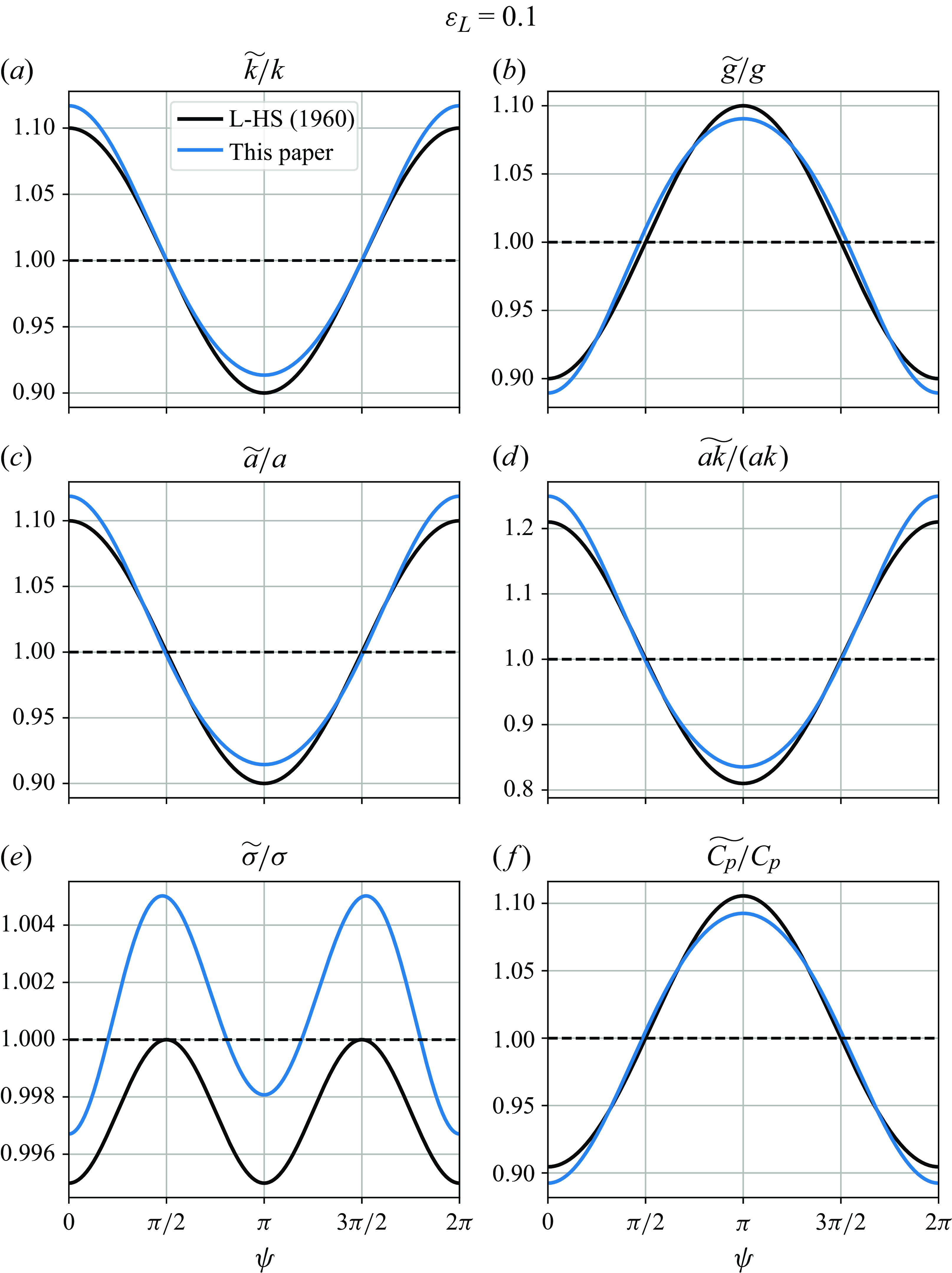
Figure 2. Steady analytical solutions for the modulation of short-wave (a) wavenumber, (b) gravitational acceleration, (c) amplitude, (d) steepness, (e) intrinsic frequency and (f) intrinsic phase speed as functions of long-wave phase for $\varepsilon _L = 0.1$
, based on Longuet-Higgins & Stewart (Reference Longuet-Higgins and Stewart1960) (L-HS 1960, black) and this paper (blue). Long-wave crest and trough are located at
$\varepsilon _L = 0.1$
, based on Longuet-Higgins & Stewart (Reference Longuet-Higgins and Stewart1960) (L-HS 1960, black) and this paper (blue). Long-wave crest and trough are located at $\psi = 0$
and
$\psi = 0$
and $\psi = \pi$
, respectively.
$\psi = \pi$
, respectively.
3.2. Gravity modulation
Three distinct effects contribute to the modulation of the effective gravity of short waves in the presence of long waves. First, long waves induce orbital (centripetal) accelerations on their surface, so the short waves ride in an accelerated reference frame and experience an effective gravity that is lower at the crests and higher in the troughs (Longuet-Higgins Reference Longuet-Higgins1986, Reference Longuet-Higgins1987). This is an ${\mathcal{O}}(\varepsilon _L)$
effect. Second, it is important to distinguish between the Eulerian and Lagrangian effective gravities (Longuet-Higgins Reference Longuet-Higgins1986). The Eulerian gravity is that which would be measured by a fixed wave staff, for example, and features sharp and strong minima at the crests and broad and weak maxima in the troughs. In contrast, the Lagrangian gravity is that which is experienced by a short-wave group that propagates with its own group speed and is advected by the ambient, long-wave-induced velocity. The Lagrangian velocity is overall smoother and more attenuated compared with its Eulerian counterpart because the local slope as experienced by the travelling short-wave group is gentler. The two gravities are related by
${\mathcal{O}}(\varepsilon _L)$
effect. Second, it is important to distinguish between the Eulerian and Lagrangian effective gravities (Longuet-Higgins Reference Longuet-Higgins1986). The Eulerian gravity is that which would be measured by a fixed wave staff, for example, and features sharp and strong minima at the crests and broad and weak maxima in the troughs. In contrast, the Lagrangian gravity is that which is experienced by a short-wave group that propagates with its own group speed and is advected by the ambient, long-wave-induced velocity. The Lagrangian velocity is overall smoother and more attenuated compared with its Eulerian counterpart because the local slope as experienced by the travelling short-wave group is gentler. The two gravities are related by
 \begin{equation} \widetilde {g_l} = g + \frac {{\textrm d}W}{{\textrm d}t} = g + \frac {\partial W}{\partial t} + \left (C_g + U\right ) \frac {\partial W}{\partial x} = \widetilde {g_e} + \left (C_g + U\right ) \frac {\partial W}{\partial x}, \end{equation}
where $l$
and
$l$
and $e$
subscripts serve to denote ‘Lagrangian’ and ‘Eulerian’, respectively. Although Longuet-Higgins (Reference Longuet-Higgins1986) thoroughly described the differences between the Eulerian and Lagrangian effective gravities, he did so for a fully nonlinear irrotational gravity wave, which can be computed numerically but not analytically. Note also that, when evaluating the Lagrangian effective gravity, Longuet-Higgins (Reference Longuet-Higgins1987) considered the orbital motion of the long wave but not the propagation speed of the short-wave group, which can exceed the ambient velocity
$e$
subscripts serve to denote ‘Lagrangian’ and ‘Eulerian’, respectively. Although Longuet-Higgins (Reference Longuet-Higgins1986) thoroughly described the differences between the Eulerian and Lagrangian effective gravities, he did so for a fully nonlinear irrotational gravity wave, which can be computed numerically but not analytically. Note also that, when evaluating the Lagrangian effective gravity, Longuet-Higgins (Reference Longuet-Higgins1987) considered the orbital motion of the long wave but not the propagation speed of the short-wave group, which can exceed the ambient velocity $U$
depending on the properties of the short and long waves considered. Group speed of the short waves aside, the Lagrangian correction to the gravity being an advective term is
$U$
depending on the properties of the short and long waves considered. Group speed of the short waves aside, the Lagrangian correction to the gravity being an advective term is ${\mathcal{O}}(\varepsilon _L^2)$
. Third, the projection of the long-wave-induced horizontal acceleration in the curvilinear coordinate system contributes small but non-negligible effects on the short-wave effective gravity (Phillips Reference Phillips1981; Zhang & Melville Reference Zhang and Melville1990). These three effects are completely described by projecting the gravitational acceleration vector from the coordinate that is perpendicular to the mean water surface (
${\mathcal{O}}(\varepsilon _L^2)$
. Third, the projection of the long-wave-induced horizontal acceleration in the curvilinear coordinate system contributes small but non-negligible effects on the short-wave effective gravity (Phillips Reference Phillips1981; Zhang & Melville Reference Zhang and Melville1990). These three effects are completely described by projecting the gravitational acceleration vector from the coordinate that is perpendicular to the mean water surface ( $z=0$
) to that which is perpendicular to the long-wave surface (
$z=0$
) to that which is perpendicular to the long-wave surface ( $z=\eta _L$
), and likewise for the long-wave orbital accelerations
$z=\eta _L$
), and likewise for the long-wave orbital accelerations
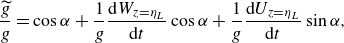 \begin{equation} \frac {\widetilde {g}}{g} = \cos {\alpha } + \frac {1}{g} \dfrac {{\textrm d}W_{z=\eta _L}}{{\textrm d}t} \cos {\alpha } + \frac {1}{g} \dfrac {{\textrm d}U_{z=\eta _L}}{{\textrm d}t} \sin {\alpha }, \end{equation}
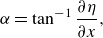 \begin{equation} \alpha = \tan ^{-1}{\dfrac {\partial \eta }{\partial x}}, \end{equation}
where $\alpha$
is the local slope of the long-wave surface. For short waves on a linear long wave, the Eulerian gravity modulation is
$\alpha$
is the local slope of the long-wave surface. For short waves on a linear long wave, the Eulerian gravity modulation is
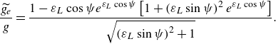 \begin{equation} \frac {\widetilde {g_e}}{g} = \frac { 1 - \varepsilon _L \cos {\psi } e^{\varepsilon _L \cos {\psi }} \left [ 1 + \left (\varepsilon _L \sin {\psi }\right )^2 e^{\varepsilon _L \cos {\psi }} \right ] } {\sqrt {\left (\varepsilon _L \sin {\psi }\right )^2 + 1}}. \end{equation}
The same derivation can be carried out for the Lagrangian gravity modulation following (3.4)–(3.6), and is omitted here for brevity. Curvilinear effects on effective gravity can be removed altogether by setting $\alpha = 0$
. In that case, (3.7) simplifies to
$\alpha = 0$
. In that case, (3.7) simplifies to
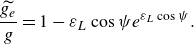 \begin{equation} \frac {\widetilde {g_e}}{g} = 1 - \varepsilon _L \cos {\psi } e^{\varepsilon _L \cos {\psi }}. \end{equation}
If we evaluate the orbital accelerations at the mean water level $z=0$
, this further simplifies to
$z=0$
, this further simplifies to
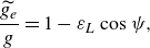 \begin{equation} \frac {\widetilde {g_e}}{g} = 1 - \varepsilon _L \cos {\psi }, \end{equation}
which is the form used by Longuet-Higgins & Stewart (Reference Longuet-Higgins and Stewart1960) and Peureux et al. (Reference Peureux, Ardhuin and Guimarães2021), for example. The Lagrangian correction in (3.4) is
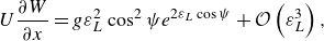 \begin{equation} U \frac {\partial W}{\partial x} = g \varepsilon _L^2 \cos ^2{\psi } e^{2 \varepsilon _L \cos {\psi }} + {\mathcal{O}}\left(\varepsilon _L^3\right), \end{equation}
and so it becomes important only for large $\varepsilon _L$
.
$\varepsilon _L$
.
The general form of the gravity modulation (3.5) is convenient because it allows us to easily attribute the modulation to different processes. It also makes it straightforward to evaluate the gravity modulation for different long-wave forms, by evaluating the orbital accelerations and the local slope for each wave form. For a third-order Stokes wave, for example, the elevation is
 \begin{equation} \eta _{St} = a_L \left [ \cos {\psi } + \dfrac {1}{2} \varepsilon _L \cos {2\psi } + \varepsilon _L^2 \left ( \dfrac {3}{8} \cos {3\psi } - \dfrac {1}{16} \cos {\psi } \right ) \right ] + {\mathcal{O}}\left(\varepsilon _L^4\right). \end{equation}
Without considering the curvilinear effects in (3.5), the gravitational acceleration at the surface of a Stokes wave is, to the third order
 \begin{equation}\begin{aligned} \frac {\widetilde {g}}{g} &= \!\left \{ 1 - \varepsilon _L e^{k \eta _{St}}\! \left [ \cos {\psi } - \varepsilon _L \sin {\psi } \!\left ( \sin {\psi } + \varepsilon _L \sin {2\psi } - \dfrac {1}{16} \varepsilon _L^2 \sin {\psi } + \dfrac {9}{8} \varepsilon _L^2 \sin {3\psi }\! \right )\! \right ]\! \right \}.\\[6pt] \end{aligned}\end{equation}
The equivalent expression that includes the curvilinear effects can be derived by evaluating the velocities and the local slope $\alpha$
at
$\alpha$
at $z = \eta _{St}$
, and inserting them into (3.5)
$z = \eta _{St}$
, and inserting them into (3.5)
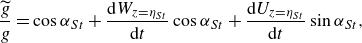 \begin{equation} \frac {\widetilde {g}}{g} = \cos {\alpha _{St}} + \dfrac {{\textrm d}W_{z=\eta _{St}}}{{\textrm d}t} \cos {\alpha _{St}} + \dfrac {{\textrm d}U_{z=\eta _{St}}}{{\textrm d}t} \sin {\alpha _{St}}, \end{equation}
 \begin{equation} \alpha _{St} = \tan ^{-1}{\dfrac {\partial \eta _{St}}{\partial x}}. \end{equation}
Let us now examine the contributions of the different terms to the short-wave effective-gravity modulation. Figure 3(a) shows the effective-gravity modulation of short waves as a function of the long-wave phase for $\varepsilon _L = 0.3$
, for a variety of the gravity modulation forms. Although quite steep, this value of
$\varepsilon _L = 0.3$
, for a variety of the gravity modulation forms. Although quite steep, this value of $\varepsilon _L$
allows easier visualisation of the modulation differences. To
$\varepsilon _L$
allows easier visualisation of the modulation differences. To ${\mathcal{O}}(\varepsilon _L)$
, the gravity modulation is out of phase with the long-wave elevation, with the short waves experiencing a lower effective gravity on the long-wave crests and a higher effective gravity in the troughs. Evaluating the orbital accelerations at
${\mathcal{O}}(\varepsilon _L)$
, the gravity modulation is out of phase with the long-wave elevation, with the short waves experiencing a lower effective gravity on the long-wave crests and a higher effective gravity in the troughs. Evaluating the orbital accelerations at $z=\eta$
and the Lagrangian gravity correction each have an
$z=\eta$
and the Lagrangian gravity correction each have an ${\mathcal{O}}(\varepsilon _L^2)$
contribution but of opposite signs. The former amplifies the gravity modulation while the latter attenuates it. The curvilinear effects are significant at the front and rear faces of the long wave but not near the crests and troughs. The long-wave surface slope has a
${\mathcal{O}}(\varepsilon _L^2)$
contribution but of opposite signs. The former amplifies the gravity modulation while the latter attenuates it. The curvilinear effects are significant at the front and rear faces of the long wave but not near the crests and troughs. The long-wave surface slope has a ${\mathcal{O}}(\varepsilon _L^2)$
effect. Naturally, the slope is exactly zero at the crests and the troughs, and its effects are largest at the front and rear faces of the long wave, where the covariance between the local slope and the horizontal accelerations is largest. Evaluating the velocities and accelerations at the surface of a third-order Stokes wave causes a correction mostly at the faces of the long wave. Finally, numerically computing the surface velocities and accelerations of a fully nonlinear wave allows us to exclude uncertainties associated with the truncation errors of the Stokes expansion at first and third orders in
${\mathcal{O}}(\varepsilon _L^2)$
effect. Naturally, the slope is exactly zero at the crests and the troughs, and its effects are largest at the front and rear faces of the long wave, where the covariance between the local slope and the horizontal accelerations is largest. Evaluating the velocities and accelerations at the surface of a third-order Stokes wave causes a correction mostly at the faces of the long wave. Finally, numerically computing the surface velocities and accelerations of a fully nonlinear wave allows us to exclude uncertainties associated with the truncation errors of the Stokes expansion at first and third orders in $\varepsilon _L$
. At this steepness, the fully nonlinear solution is marginally different from that of the third-order Stokes wave (see also Appendix B for the errors in surface velocity estimates of the linear and third-order Stokes approximations).
$\varepsilon _L$
. At this steepness, the fully nonlinear solution is marginally different from that of the third-order Stokes wave (see also Appendix B for the errors in surface velocity estimates of the linear and third-order Stokes approximations).
Figure 3. Analytical solutions for the effective gravitational acceleration modulation by long waves, as functions of the long-wave phase, for $\varepsilon _L = 0.3$
. Black is for Eulerian gravity of a linear wave evaluated at
$\varepsilon _L = 0.3$
. Black is for Eulerian gravity of a linear wave evaluated at $z=0$
; blue is the same as black but evaluated at
$z=0$
; blue is the same as black but evaluated at $z=\eta$
; orange is the same as blue but for Lagrangian gravity; green is the same as orange but in a curvilinear reference frame; red is the same as green but for a third-order Stokes wave; and purple is the same as red but for a fully nonlinear wave. The elevation and surface velocities for the fully nonlinear wave are computed following Clamond & Dutykh (Reference Clamond and Dutykh2018). Long-wave crest and trough are located at
$z=\eta$
; orange is the same as blue but for Lagrangian gravity; green is the same as orange but in a curvilinear reference frame; red is the same as green but for a third-order Stokes wave; and purple is the same as red but for a fully nonlinear wave. The elevation and surface velocities for the fully nonlinear wave are computed following Clamond & Dutykh (Reference Clamond and Dutykh2018). Long-wave crest and trough are located at $\psi = 0$
and
$\psi = 0$
and $\psi = \pi$
, respectively.
$\psi = \pi$
, respectively.
It is instructive to also examine the minimum values of the effective gravity as functions of long-wave steepness $\varepsilon _L$
(figure 4), as the minima occur at or near the long-wave crests where the short-wave modulation is largest. Without the Lagrangian correction to the effective gravity, the gravity modulation is overestimated; for accelerations evaluated at the surface of a linear wave, the maximum gravity reduction is 60 % at
$\varepsilon _L$
(figure 4), as the minima occur at or near the long-wave crests where the short-wave modulation is largest. Without the Lagrangian correction to the effective gravity, the gravity modulation is overestimated; for accelerations evaluated at the surface of a linear wave, the maximum gravity reduction is 60 % at $\varepsilon _L = 0.4$
. The Lagrangian correction attenuates the gravity modulation, making the gravity reduction at the crests
$\varepsilon _L = 0.4$
. The Lagrangian correction attenuates the gravity modulation, making the gravity reduction at the crests $\approx 25\, \%$
. As the slope effects on the effective gravity exist only away from crests and troughs, they may be neglected in the steady solutions where modulation is typically evaluated at the long-wave crests. Here, the slope effect causes a difference in the minimum effective gravity for
$\approx 25\, \%$
. As the slope effects on the effective gravity exist only away from crests and troughs, they may be neglected in the steady solutions where modulation is typically evaluated at the long-wave crests. Here, the slope effect causes a difference in the minimum effective gravity for $\varepsilon _L \gtrsim 0.3$
. The effective-gravity reduction at the crests in the case of a fully nonlinear wave is
$\varepsilon _L \gtrsim 0.3$
. The effective-gravity reduction at the crests in the case of a fully nonlinear wave is $\approx$
10 %, 19 %, 27 % and 40 %, for
$\approx$
10 %, 19 %, 27 % and 40 %, for $\varepsilon _L$
of 0.1, 0.2, 0.3 and 0.4, respectively. These are similar to the fully nonlinear numerical estimates of Longuet-Higgins (Reference Longuet-Higgins1986, Reference Longuet-Higgins1987).
$\varepsilon _L$
of 0.1, 0.2, 0.3 and 0.4, respectively. These are similar to the fully nonlinear numerical estimates of Longuet-Higgins (Reference Longuet-Higgins1986, Reference Longuet-Higgins1987).

Figure 4. As figure 3 but showing the minimum short-wave gravity modulation as a function of long-wave steepness $\varepsilon _L$
.
$\varepsilon _L$
.
3.3. Amplitude and steepness modulation
The modulation of short-wave amplitude can be derived in a similar way as we did for the wavenumber, except that here we linearise the wave action balance (2.6) and integrate it in time
 \begin{equation} \frac {\widetilde {N}}{N} = e^{\varepsilon _L \cos {\psi } e^{\varepsilon _L \cos {\psi }}}. \end{equation}
Since wave action is energy divided by the intrinsic frequency $\sigma$
, and energy scales with
$\sigma$
, and energy scales with $ga^2$
, the modulation of the amplitude is related to the modulations of gravity, wavenumber and action
$ga^2$
, the modulation of the amplitude is related to the modulations of gravity, wavenumber and action
 \begin{equation} \dfrac {\widetilde {a}}{a} = \sqrt { \dfrac {g}{\widetilde {g}} \dfrac {\widetilde {\sigma }}{\sigma } \dfrac {\widetilde {N}}{N}} = \left ( \dfrac {\widetilde {k}}{k} \right )^{\frac {1}{4}} \left ( \dfrac {\widetilde {N}}{N} \right )^{\frac {1}{2}} \left ( \dfrac {\widetilde {g}}{g} \right )^{-\frac {1}{4}}. \end{equation}
To ${\mathcal{O}}(\varepsilon _L)$
, and using (3.2) and (3.15), the above simplifies to the result of Longuet-Higgins & Stewart (Reference Longuet-Higgins and Stewart1960)
${\mathcal{O}}(\varepsilon _L)$
, and using (3.2) and (3.15), the above simplifies to the result of Longuet-Higgins & Stewart (Reference Longuet-Higgins and Stewart1960)
 \begin{equation} \dfrac {\widetilde {a}}{a} = \left ( \dfrac {\widetilde {g}}{g} \right )^{-\frac {1}{4}} \left ( 1 + \varepsilon _L \right )^{\frac {3}{4}} \approx \frac {(1 + \varepsilon _L)^{\frac {3}{4}}}{(1 - \varepsilon _L)^{\frac {1}{4}}} \approx 1 + \varepsilon _L. \end{equation}
The amplitude and steepness modulation of the short waves as a function of the long-wave phase for $\varepsilon _L = 0.1$
are compared with the Longuet-Higgins & Stewart (Reference Longuet-Higgins and Stewart1960) solutions in figures 2(c) and 2(d), respectively. Also shown are the modulation of the short-wave intrinsic frequency and phase speed in panels (e) and (f), respectively. As the wavenumber and gravity modulations are both
$\varepsilon _L = 0.1$
are compared with the Longuet-Higgins & Stewart (Reference Longuet-Higgins and Stewart1960) solutions in figures 2(c) and 2(d), respectively. Also shown are the modulation of the short-wave intrinsic frequency and phase speed in panels (e) and (f), respectively. As the wavenumber and gravity modulations are both ${\mathcal{O}}(\varepsilon _L)$
and out of phase, the intrinsic frequency modulation is
${\mathcal{O}}(\varepsilon _L)$
and out of phase, the intrinsic frequency modulation is ${\mathcal{O}}(\varepsilon _L^2)$
, positive on the long-wave faces and negative on the crests and troughs. For the short-wave phase speed modulation, the wavenumber and gravity modulations work in tandem and cause the short-wave phase speed to be reduced on the long-wave crests and increased in the troughs.
${\mathcal{O}}(\varepsilon _L^2)$
, positive on the long-wave faces and negative on the crests and troughs. For the short-wave phase speed modulation, the wavenumber and gravity modulations work in tandem and cause the short-wave phase speed to be reduced on the long-wave crests and increased in the troughs.
Finally, the short-wave steepness modulation follows from (3.16)
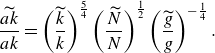 \begin{equation} \dfrac {\widetilde {ak}}{ak} = \left ( \dfrac {\widetilde {k}}{k} \right )^{\frac {5}{4}} \left ( \dfrac {\widetilde {N}}{N} \right )^{\frac {1}{2}} \left ( \dfrac {\widetilde {g}}{g} \right )^{-\frac {1}{4}}. \end{equation}
The short-wave steepness modulation at the long-wave crests is thus largely controlled by the wavenumber modulation (5/8 or 62.5 %), followed by the convergence of wave action (1/4 or 25 %), and by least amount by the effective-gravity reduction (1/8 or 12.5 %) (figure 5). Equation (3.18) and figure 5 demonstrate that more than half of the steepness modulation can be captured by the wavenumber modulation alone. Further, considering the wavenumber and wave action modulations, while neglecting the gravity modulation, captures $\approx$
88 % of the steepness modulation at the long-wave crests. This result may be useful for the interpretation of remote sensing products that resolve some but not all of the short-wave modulation effects. Finally, the relative contributions of different modulation factors remain mostly constant as
$\approx$
88 % of the steepness modulation at the long-wave crests. This result may be useful for the interpretation of remote sensing products that resolve some but not all of the short-wave modulation effects. Finally, the relative contributions of different modulation factors remain mostly constant as $\varepsilon _L$
increases, with only a mild decrease of the effective-gravity modulation contribution, and mild increases of the wavenumber and wave action modulation contributions.
$\varepsilon _L$
increases, with only a mild decrease of the effective-gravity modulation contribution, and mild increases of the wavenumber and wave action modulation contributions.

Figure 5. Contributions of short-wave wavenumber, action and effective-gravity modulations to the steepness modulation, as functions of the long-wave steepness $\varepsilon _L$
. Panel (a) shows each modulation factor (colour) and their product (black), and panel (b) shows their relative contributions in percentage, calculated as the ratio of the logarithm of each modulation factor to the logarithm of the product of all modulations.
$\varepsilon _L$
. Panel (a) shows each modulation factor (colour) and their product (black), and panel (b) shows their relative contributions in percentage, calculated as the ratio of the logarithm of each modulation factor to the logarithm of the product of all modulations.
3.4. Limits to the wave action conservation
Following the variational approach by Whitham (Reference Whitham1965), Bretherton & Garrett (Reference Bretherton and Garrett1968) showed that the wave action is conserved for small-amplitude (linear) waves that propagate in slowly varying media. Longuet-Higgins (Reference Longuet-Higgins1987) correctly pointed out both requirements – that both the medium and the short-wave train must be slowly varying – for the wave action conservation to hold. However, he incorrectly stated that there is no explicit restriction on the steepness of the long wave, and that it appears necessary to only assume small-amplitude short waves and significant scale separation ( $k/k_L$
). The restriction on
$k/k_L$
). The restriction on $\varepsilon _L$
becomes apparent when we recognise that the long wave-induced orbital velocity scales with
$\varepsilon _L$
becomes apparent when we recognise that the long wave-induced orbital velocity scales with $\varepsilon _L$
, and that the divergence of this velocity is the dominant term in (2.5) and (2.6). Here, we show that in the general case both the homogeneity and the stationarity of a short-wave quantity
$\varepsilon _L$
, and that the divergence of this velocity is the dominant term in (2.5) and (2.6). Here, we show that in the general case both the homogeneity and the stationarity of a short-wave quantity $q$
depend on the long-wave steepness
$q$
depend on the long-wave steepness $\varepsilon _L$
.
$\varepsilon _L$
.
The homogeneity and stationarity of a scalar quantity $q$
can be expressed as conditions on the instantaneous fractional rate of change of
$q$
can be expressed as conditions on the instantaneous fractional rate of change of $q$
being much smaller than the short-wave inverse scales
$q$
being much smaller than the short-wave inverse scales
 \begin{equation} \frac {1}{q} \frac {\partial q}{\partial x} \ll k, \end{equation}
 \begin{equation} \frac {1}{q} \frac {\partial q}{\partial t} \ll \sigma. \end{equation}
The slowly varying conditions on the medium (in our case, the long-wave orbital velocity U) are then
 \begin{equation} \frac {1}{U} \frac {\partial U}{\partial x} \ll \widetilde {k}, \end{equation}
 \begin{equation} \frac {1}{U} \frac {\partial U}{\partial t} \ll \widetilde {\sigma }, \end{equation}
respectively. For a linear long wave, these conditions are equivalent to the scale separation between the long and short waves
 \begin{equation} k_L \ll \widetilde {k}, \end{equation}
 \begin{equation} \sigma _L \ll \widetilde {\sigma }. \end{equation}
Bretherton & Garrett (Reference Bretherton and Garrett1968) also require that the medium is nearly uniform over the vertical scales of motion of the short waves
 \begin{equation} \frac {1}{U} \frac {\partial U}{\partial z} \ll \widetilde {k}, \end{equation}
which, for a long deep-water wave, is equivalent to (3.23). Alternatively, if we use the second Froude number criterion following Ellingsen (Reference Ellingsen2014) and quantify the shear length under the long-wave surface as
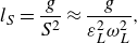 \begin{equation} l_S = \frac {g}{S^2} \approx \frac {g}{\varepsilon _L^2 \omega _L^2}, \end{equation}
we arrive at an additional requirement
 \begin{equation} \frac {k}{k_L} \gg \varepsilon _L^2, \end{equation}
which relates the scale separation to the long-wave steepness.
Now, to address the variation of short-wave properties, we apply (3.19)–(3.20) to the long-wave phase-dependent wavenumber, gravitational acceleration and wave action, and define the homogeneity and stationarity as
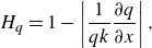 \begin{equation} H_q = 1 - \left | \frac {1}{qk} \frac {\partial q}{\partial x} \right |, \end{equation}
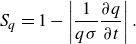 \begin{equation} S_q = 1 - \left | \frac {1}{q\sigma } \frac {\partial q}{\partial t} \right |. \end{equation}
With the above definitions, we consider $q$
to be homogeneous and stationary as
$q$
to be homogeneous and stationary as $H_q \rightarrow 1$
and
$H_q \rightarrow 1$
and $S_q \rightarrow 1$
, respectively.
$S_q \rightarrow 1$
, respectively.
For the linearised modulation solutions (3.2), (3.9) and (3.15), the respective homogeneity expressions are
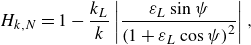 \begin{equation} H_{k,N} = 1 - \frac {k_L}{k} \left | \frac {\varepsilon _L \sin {\psi }}{\left (1 + \varepsilon _L \cos {\psi }\right )^2} \right |, \end{equation}
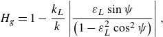 \begin{equation} H_{g} = 1 - \frac {k_L}{k} \left | \frac {\varepsilon _L \sin {\psi }}{\left (1 - \varepsilon _L^2 \cos ^2{\psi }\right )} \right |, \end{equation}
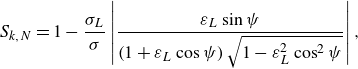 \begin{equation} S_{k,N} = 1 - \frac {\sigma _L}{\sigma } \left | \frac {\varepsilon _L \sin {\psi }}{\left (1 + \varepsilon _L \cos {\psi }\right ) \sqrt {1 - \varepsilon _L^2 \cos ^2{\psi }}} \right |, \end{equation}
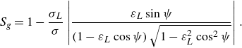 \begin{equation} S_{g} = 1 - \frac {\sigma _L}{\sigma } \left | \frac {\varepsilon _L \sin {\psi }}{\left (1 - \varepsilon _L \cos {\psi }\right ) \sqrt {1 - \varepsilon _L^2 \cos ^2{\psi }}} \right |. \end{equation}
The steady, linearised solutions thus depend on both the wavenumber ratio $k_L/k$
(homogeneity) or the frequency ratio
$k_L/k$
(homogeneity) or the frequency ratio $\sigma _L/\sigma$
(stationarity) and the long-wave steepness
$\sigma _L/\sigma$
(stationarity) and the long-wave steepness $\varepsilon _L$
.
$\varepsilon _L$
.
Figure 6 shows the homogeneities and stationarities of the short-wave wavenumber and effective gravity based on the steady solutions and their derived criteria as minima of (3.19)–(3.20). Stationarity is a stronger requirement than homogeneity. At the lowest scale separation considered ( $k/k_L = 10$
), short-wave wavenumber, action and effective gravity are all strongly homogeneous (
$k/k_L = 10$
), short-wave wavenumber, action and effective gravity are all strongly homogeneous ( $H_{k,N,g} \gt 0.99$
) for
$H_{k,N,g} \gt 0.99$
) for $\varepsilon _L \lt 0.1$
. However, the solutions are only strongly stationary (
$\varepsilon _L \lt 0.1$
. However, the solutions are only strongly stationary ( $S_{k,N,g} \gt 0.99$
) at a high scale separation of
$S_{k,N,g} \gt 0.99$
) at a high scale separation of $k/k_L = 100$
for
$k/k_L = 100$
for $\varepsilon _L \lt 0.1$
. If we consider weakly stationary conditions as
$\varepsilon _L \lt 0.1$
. If we consider weakly stationary conditions as $S_{k,N,g} \gt 0.9$
, then the solutions satisfy the requirements for the wave action conservation for
$S_{k,N,g} \gt 0.9$
, then the solutions satisfy the requirements for the wave action conservation for $\varepsilon _L \lt 0.3$
at
$\varepsilon _L \lt 0.3$
at $k/k_L = 10$
, and for
$k/k_L = 10$
, and for $\varepsilon _L \lt 0.4$
at
$\varepsilon _L \lt 0.4$
at $k/k_L \gt 20$
. Although Bretherton & Garrett (Reference Bretherton and Garrett1968) state that the wave action balance is valid to
$k/k_L \gt 20$
. Although Bretherton & Garrett (Reference Bretherton and Garrett1968) state that the wave action balance is valid to ${\mathcal{O}}(k_L/k)$
, applying the general criteria (3.19)–(3.20) yields an error of
${\mathcal{O}}(k_L/k)$
, applying the general criteria (3.19)–(3.20) yields an error of ${\mathcal{O}}(\varepsilon _L k_L/k)$
. We will revisit these criteria based on the numerical solutions of nonlinear wave action and crest conservation equations in the next section. For the asymptotic limits of wave action conservation in terms of the wave short-wave steepness, see Appendix A.3.
${\mathcal{O}}(\varepsilon _L k_L/k)$
. We will revisit these criteria based on the numerical solutions of nonlinear wave action and crest conservation equations in the next section. For the asymptotic limits of wave action conservation in terms of the wave short-wave steepness, see Appendix A.3.
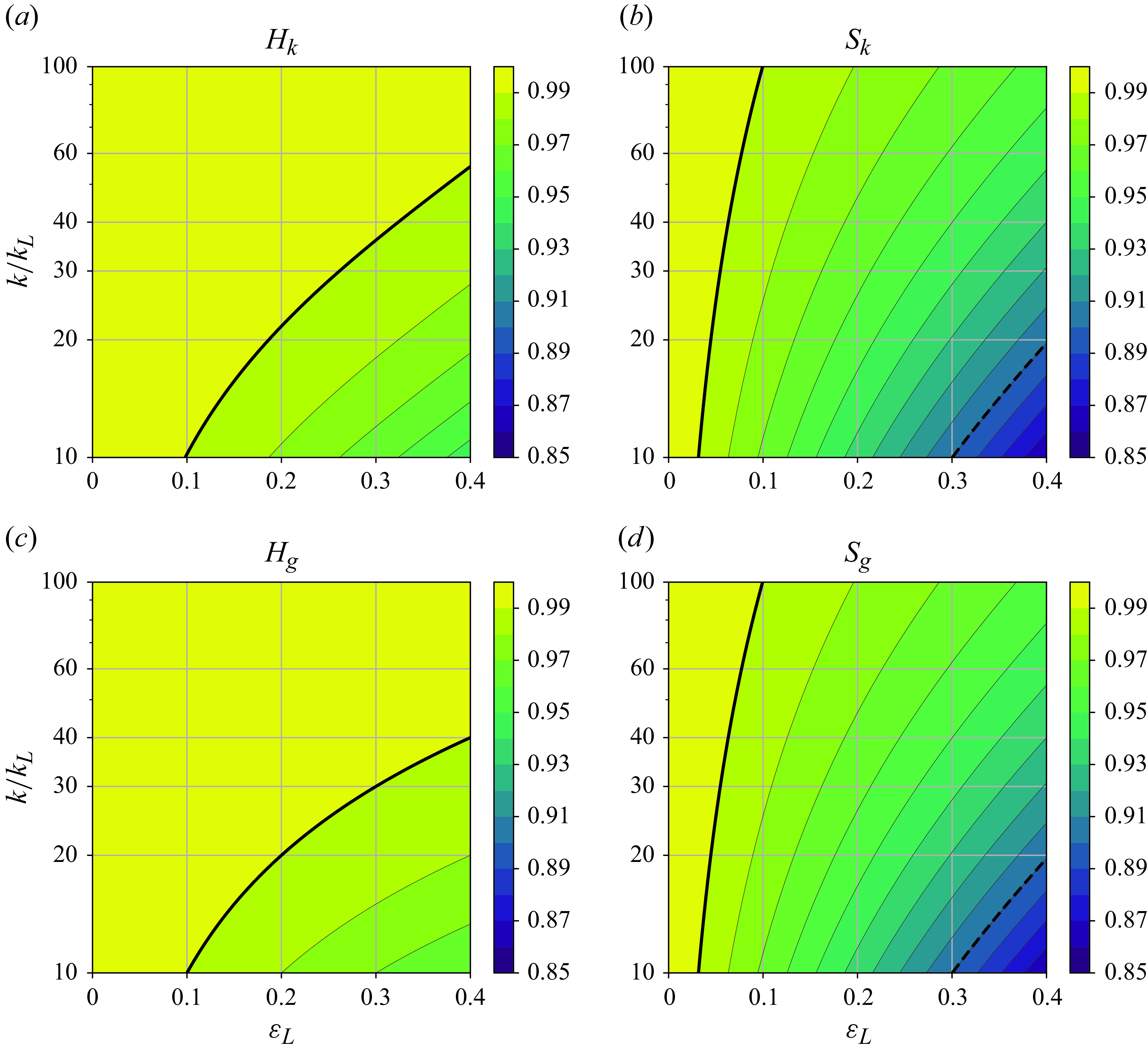
Figure 6. Homogeneity (left) and stationarity (right) of the short-wave wavenumber (a), (b) and effective gravity (c), (d) as a function of the long-wave steepness $\varepsilon _L$
and the wavenumber ratio
$\varepsilon _L$
and the wavenumber ratio $k/k_L$
, based on the linearised solutions (3.30)–(3.33). Solid and dashed lines highlight the 0.99 and 0.90 values, respectively.
$k/k_L$
, based on the linearised solutions (3.30)–(3.33). Solid and dashed lines highlight the 0.99 and 0.90 values, respectively.
4. Numerical solutions
4.1. Model description
To quantify the contribution of the nonlinear terms in (2.5) and (2.6), and to evaluate the steadiness assumption of the analytical solutions, we now proceed to numerically integrate the full set of crest and action conservation equations. Equations (2.5) and (2.6) are discretised using second-order central finite difference in space and integrated in time using the fourth-order Runge–Kutta method (Butcher & Wanner Reference Butcher and Wanner1996). The space is divided into 128 grid points. This is effectively the same equation set and numerical configuration as those of Peureux et al. (Reference Peureux, Ardhuin and Guimarães2021), except that their long-wave orbital velocities are evaluated at $z=0$
instead of
$z=0$
instead of $z=\eta _L$
, thus neglecting the Stokes drift induced by long waves on short-wave groups (Stokes Reference Stokes1847; van den Bremer & Breivik Reference van den Bremer and Breivik2018; Monismith Reference Monismith2020). Their gravity modulation also does not consider the nonlinear, Lagrangian or slope effects, however, this difference does not qualitatively affect the results. Another difference is the choice of the numerical scheme for spatial differences, which in their case is the more sophisticated 4th order Monotonic Upstream-centered Scheme for Conservation Laws scheme (Kurganov & Tadmor Reference Kurganov and Tadmor2000). Although the second-order central finite difference is not appropriate for many numerical problems, in our case it is sufficient because it is conservative and the fields that we compute derivatives of are smooth and continuous. The maximum relative error of the centred finite difference in this model is
$z=\eta _L$
, thus neglecting the Stokes drift induced by long waves on short-wave groups (Stokes Reference Stokes1847; van den Bremer & Breivik Reference van den Bremer and Breivik2018; Monismith Reference Monismith2020). Their gravity modulation also does not consider the nonlinear, Lagrangian or slope effects, however, this difference does not qualitatively affect the results. Another difference is the choice of the numerical scheme for spatial differences, which in their case is the more sophisticated 4th order Monotonic Upstream-centered Scheme for Conservation Laws scheme (Kurganov & Tadmor Reference Kurganov and Tadmor2000). Although the second-order central finite difference is not appropriate for many numerical problems, in our case it is sufficient because it is conservative and the fields that we compute derivatives of are smooth and continuous. The maximum relative error of the centred finite difference in this model is $\approx 0.066\, \%$
. The wavenumber and wave action are conservative over time within
$\approx 0.066\, \%$
. The wavenumber and wave action are conservative over time within ${\mathcal{O}}(10^{-7})$
and
${\mathcal{O}}(10^{-7})$
and ${\mathcal{O}}(10^{-5})$
relative error, respectively. We show in the next subsection that our numerical solutions for infinite long-wave trains are qualitatively equivalent to those of Peureux et al. (Reference Peureux, Ardhuin and Guimarães2021).
${\mathcal{O}}(10^{-5})$
relative error, respectively. We show in the next subsection that our numerical solutions for infinite long-wave trains are qualitatively equivalent to those of Peureux et al. (Reference Peureux, Ardhuin and Guimarães2021).
The numerical equations here are integrated in a fixed reference frame with periodic boundary conditions, rather than that moving with the long-wave phase speed. Either approach produces equivalent modulation results, however, a fixed reference frame allows for a more intuitive interpretation of the results. This difference is important to keep in mind when comparing the results of Peureux et al. (Reference Peureux, Ardhuin and Guimarães2021) and those presented here; in their figure 1 the long-wave phase is fixed and the short waves are moving leftward with the speed of $C_{pL} - C_g - U$
(neglecting group speed inhomogeneity), whereas in the figures that follow, the long wave is moving rightward with its phase speed
$C_{pL} - C_g - U$
(neglecting group speed inhomogeneity), whereas in the figures that follow, the long wave is moving rightward with its phase speed $C_{pL}$
and the short waves (that is, their action) are moving rightward with the speed of
$C_{pL}$
and the short waves (that is, their action) are moving rightward with the speed of $C_g + U$
(neglecting group speed inhomogeneity). The crest and action conservation equations are integrated in the curvilinear coordinate system in which the horizontal coordinate follows the long-wave surface, akin to Zhang & Melville (Reference Zhang and Melville1990).
$C_g + U$
(neglecting group speed inhomogeneity). The crest and action conservation equations are integrated in the curvilinear coordinate system in which the horizontal coordinate follows the long-wave surface, akin to Zhang & Melville (Reference Zhang and Melville1990).
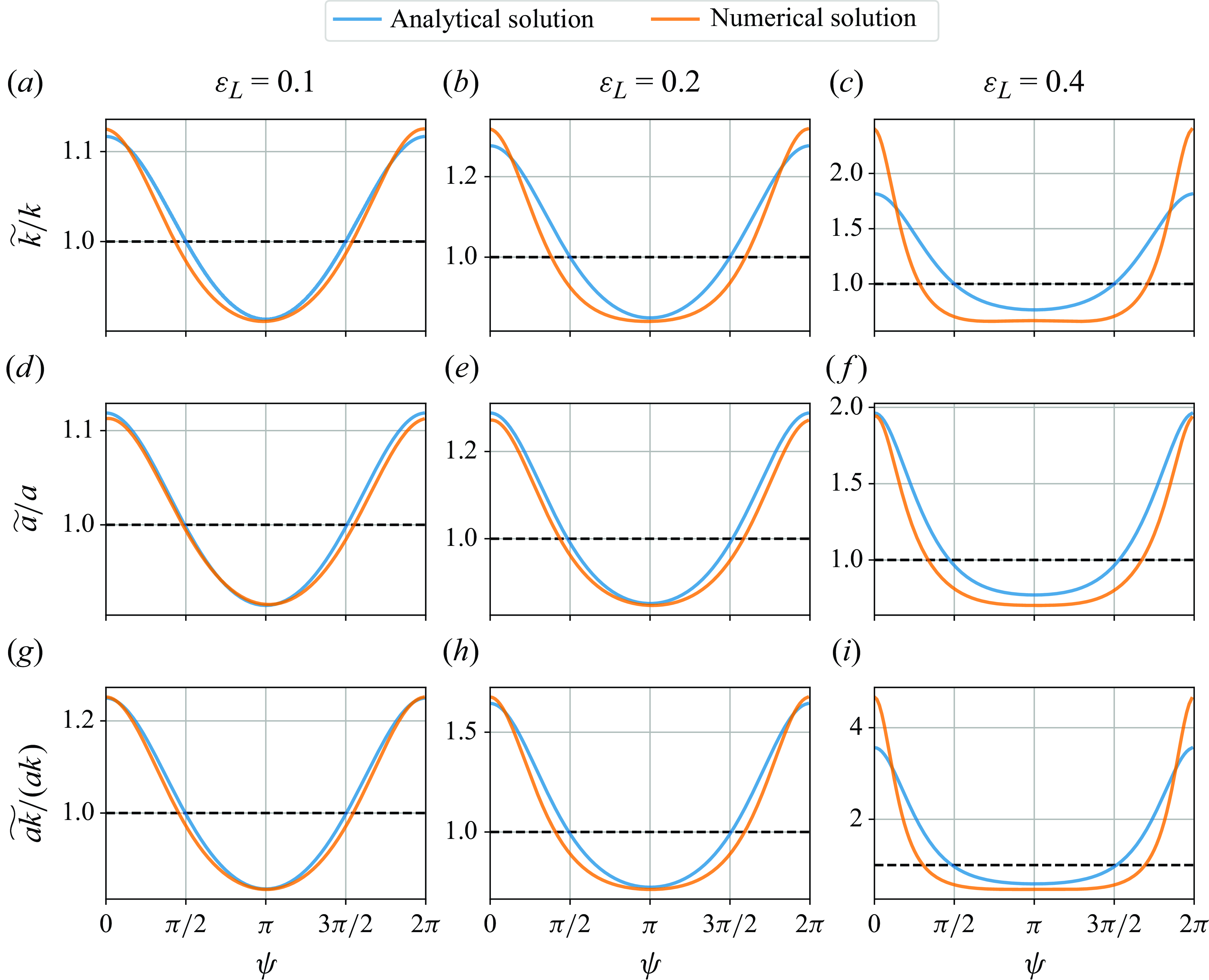
Figure 7. Comparison of numerical solutions (orange) of wavenumber (a), (b), (c), amplitude (d), (e), (f) and steepness (g), (h), (i) modulation with their analytical solutions (blue), for $\varepsilon _L$
= 0.1, 0.2 and 0.4.
$\varepsilon _L$
= 0.1, 0.2 and 0.4.
4.2. Comparison with analytical solutions
The first set of simulations is performed for the long-wave steepness of $\varepsilon _L = 0.1$
,
$\varepsilon _L = 0.1$
, $0.2$
and
$0.2$
and $0.4$
(figure 7). The long-waves are initialised from rest (
$0.4$
(figure 7). The long-waves are initialised from rest ( $a_L = 0$
) and gradually ramped up to their target steepness over 5 long-wave periods to allow for a gentle increase of the long-wave forcing on the short waves (the importance of which we discuss in more detail in the next subsection). At
$a_L = 0$
) and gradually ramped up to their target steepness over 5 long-wave periods to allow for a gentle increase of the long-wave forcing on the short waves (the importance of which we discuss in more detail in the next subsection). At $\varepsilon _L = 0.1$
, the numerical solutions for the wavenumber, amplitude and steepness modulation are all remarkably similar to the analytical solutions (figure 7
a,d,g). This suggests that for low
$\varepsilon _L = 0.1$
, the numerical solutions for the wavenumber, amplitude and steepness modulation are all remarkably similar to the analytical solutions (figure 7
a,d,g). This suggests that for low $\varepsilon _L$
the steady analytical solution is a reasonable approximation for the nonlinear crest-action solutions. The numerical solutions diverge more notably from the analytical ones at moderate
$\varepsilon _L$
the steady analytical solution is a reasonable approximation for the nonlinear crest-action solutions. The numerical solutions diverge more notably from the analytical ones at moderate $\varepsilon _L = 0.2$
(figure 7
b,e,h), and are considerably different at very high
$\varepsilon _L = 0.2$
(figure 7
b,e,h), and are considerably different at very high $\varepsilon _L = 0.4$
(figure 7
c,f,i). These differences suggest that at high
$\varepsilon _L = 0.4$
(figure 7
c,f,i). These differences suggest that at high $\varepsilon _L$
the inhomogeneity of gravitational acceleration and group speed, otherwise ignored in the steady solutions, become important.
$\varepsilon _L$
the inhomogeneity of gravitational acceleration and group speed, otherwise ignored in the steady solutions, become important.
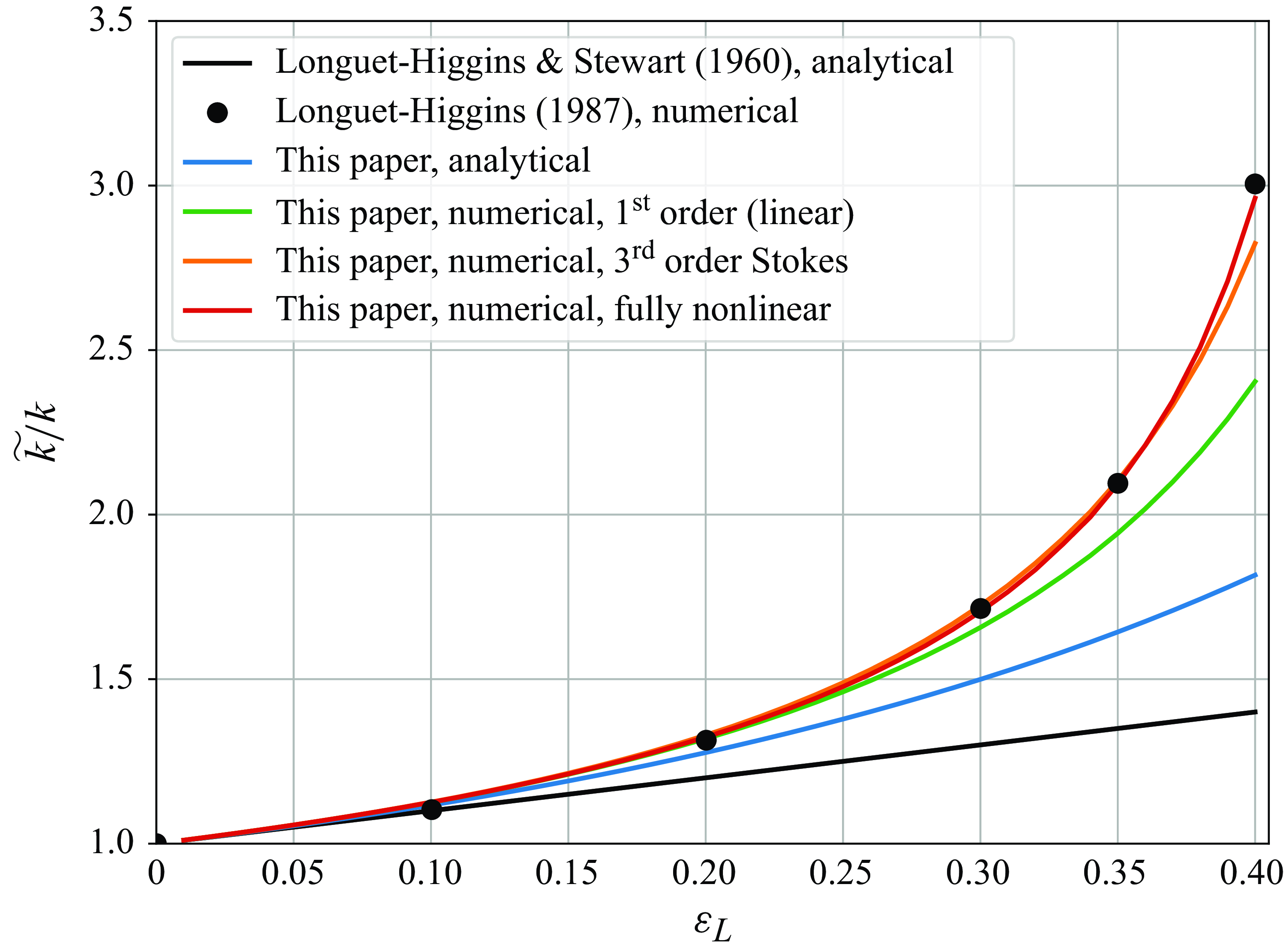
Figure 8. Maximum wavenumber modulation as a function of long-wave steepness $\varepsilon _L$
. Black line and circles are for the analytical and numerical solutions from Longuet-Higgins & Stewart (Reference Longuet-Higgins and Stewart1960) and Longuet-Higgins (Reference Longuet-Higgins1987), respectively. Blue line is based on the analytical solutions from this paper. Green and orange lines are for the numerical solutions from this paper using the linear and third-order Stokes approximations of long waves, respectively. Red line is for the fully nonlinear gravity wave based on Clamond & Dutykh (Reference Clamond and Dutykh2018).
$\varepsilon _L$
. Black line and circles are for the analytical and numerical solutions from Longuet-Higgins & Stewart (Reference Longuet-Higgins and Stewart1960) and Longuet-Higgins (Reference Longuet-Higgins1987), respectively. Blue line is based on the analytical solutions from this paper. Green and orange lines are for the numerical solutions from this paper using the linear and third-order Stokes approximations of long waves, respectively. Red line is for the fully nonlinear gravity wave based on Clamond & Dutykh (Reference Clamond and Dutykh2018).
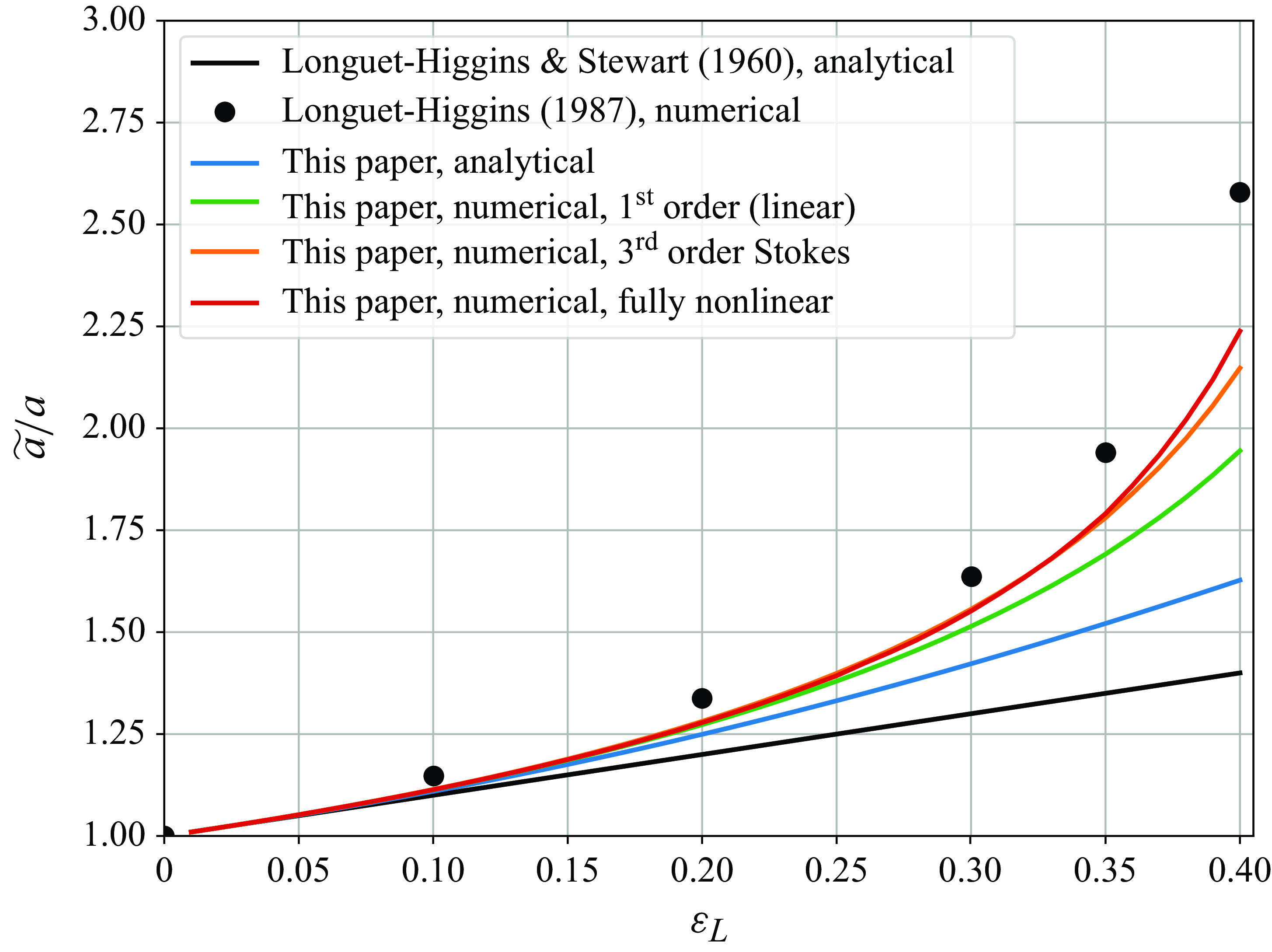
Figure 9. As figure 8 but for the amplitude modulation.
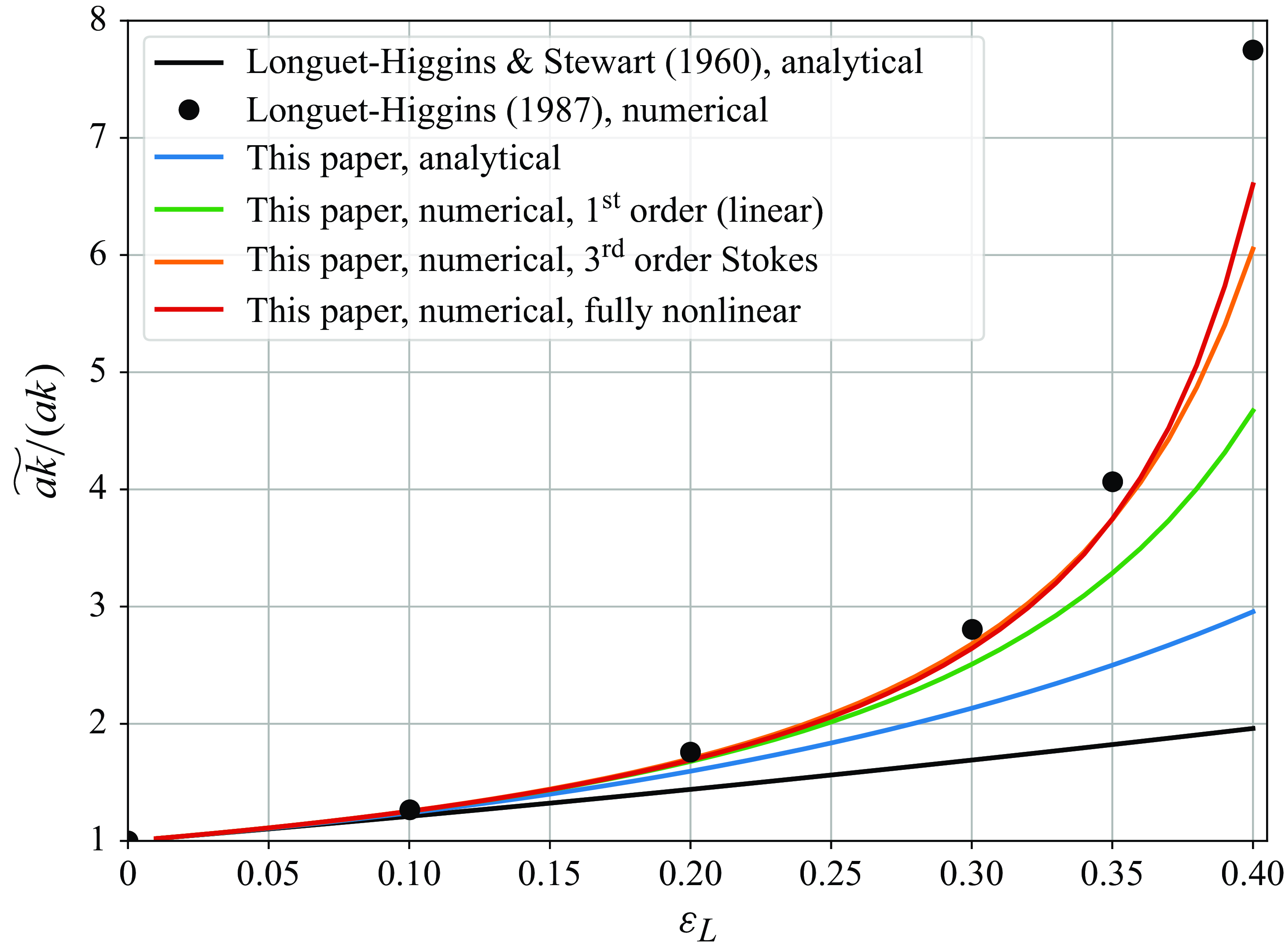
Figure 10. As figure 8 but for the steepness modulation.
The maximum modulations of the short-wave wavenumber, amplitude and steepness from the analytical and numerical solutions, are shown in figures 8, 9 and 10, respectively, as functions of the long-wave steepness $\varepsilon _L$
. Overall, the numerical solutions, based on the linear and the third-order Stokes long waves alike, begin to diverge from the analytical solution at
$\varepsilon _L$
. Overall, the numerical solutions, based on the linear and the third-order Stokes long waves alike, begin to diverge from the analytical solution at $\varepsilon _L \approx 0.15$
. The numerical solution using the third-order Stokes long wave is quantitatively very similar to the fully nonlinear solutions of Longuet-Higgins (Reference Longuet-Higgins1987) in wavenumber modulation, however, with somewhat lower amplitude and steepness modulations. Using the velocity and gravity properties of a fully nonlinear wave, based on the approach by Clamond & Dutykh (Reference Clamond and Dutykh2018), the numerical solutions diverge from those of the third-order Stokes wave only at very large steepnesses (
$\varepsilon _L \approx 0.15$
. The numerical solution using the third-order Stokes long wave is quantitatively very similar to the fully nonlinear solutions of Longuet-Higgins (Reference Longuet-Higgins1987) in wavenumber modulation, however, with somewhat lower amplitude and steepness modulations. Using the velocity and gravity properties of a fully nonlinear wave, based on the approach by Clamond & Dutykh (Reference Clamond and Dutykh2018), the numerical solutions diverge from those of the third-order Stokes wave only at very large steepnesses ( $\varepsilon _L \gt 0.3$
). Using a fully nonlinear form of the long-wave thus does not collapse the difference between the solutions here and those of Longuet-Higgins (Reference Longuet-Higgins1987). For example, at
$\varepsilon _L \gt 0.3$
). Using a fully nonlinear form of the long-wave thus does not collapse the difference between the solutions here and those of Longuet-Higgins (Reference Longuet-Higgins1987). For example, at $\varepsilon _L = 0.4$
, the steepness modulation in our solution is 6.6, whereas Longuet-Higgins (Reference Longuet-Higgins1987) finds it to be 7.8. A possible reason for this difference is that the solutions by Longuet-Higgins (Reference Longuet-Higgins1987) are stationary (see his § 2), whereas in our numerical model we solve the prognostic nonlinear equations for the short-wave wavenumber and action. As we will see in the next section, and as was suggested by Peureux et al. (Reference Peureux, Ardhuin and Guimarães2021), they are often, but not always, mostly steady, and can be strongly unsteady in special cases. Nevertheless, the overall steepness modulation between the two numerical approaches are remarkably similar, and either solution would cause the short waves of moderate steepness to break (Banner & Peregrine Reference Banner and Peregrine1993). Specifically, where the two modulation solutions differ (
$\varepsilon _L = 0.4$
, the steepness modulation in our solution is 6.6, whereas Longuet-Higgins (Reference Longuet-Higgins1987) finds it to be 7.8. A possible reason for this difference is that the solutions by Longuet-Higgins (Reference Longuet-Higgins1987) are stationary (see his § 2), whereas in our numerical model we solve the prognostic nonlinear equations for the short-wave wavenumber and action. As we will see in the next section, and as was suggested by Peureux et al. (Reference Peureux, Ardhuin and Guimarães2021), they are often, but not always, mostly steady, and can be strongly unsteady in special cases. Nevertheless, the overall steepness modulation between the two numerical approaches are remarkably similar, and either solution would cause the short waves of moderate steepness to break (Banner & Peregrine Reference Banner and Peregrine1993). Specifically, where the two modulation solutions differ ( $\varepsilon _L \gtrsim 0.3$
), the steepness modulation approaches and exceeds 3. Tripling the short-wave steepness of even
$\varepsilon _L \gtrsim 0.3$
), the steepness modulation approaches and exceeds 3. Tripling the short-wave steepness of even $\varepsilon = 0.1$
would bring the wave train near the observed breaking thresholds of
$\varepsilon = 0.1$
would bring the wave train near the observed breaking thresholds of $\varepsilon \gtrsim 0.32$
(Perlin, Choi & Tian Reference Perlin, Choi and Tian2013), although recent measurements show evidence of significantly higher breaking thresholds (Toffoli et al. Reference Toffoli, Babanin, Onorato and Waseda2010; McAllister et al. Reference McAllister, Draycott, Calvert, Davey, Dias and van den Bremer2024), even exceeding the geometric Stokes limit of 0.44. Nevertheless, in the cases where the short waves would survive the modulation and persist over multiple long-wave periods, the two solutions are effectively equivalent.
$\varepsilon \gtrsim 0.32$
(Perlin, Choi & Tian Reference Perlin, Choi and Tian2013), although recent measurements show evidence of significantly higher breaking thresholds (Toffoli et al. Reference Toffoli, Babanin, Onorato and Waseda2010; McAllister et al. Reference McAllister, Draycott, Calvert, Davey, Dias and van den Bremer2024), even exceeding the geometric Stokes limit of 0.44. Nevertheless, in the cases where the short waves would survive the modulation and persist over multiple long-wave periods, the two solutions are effectively equivalent.
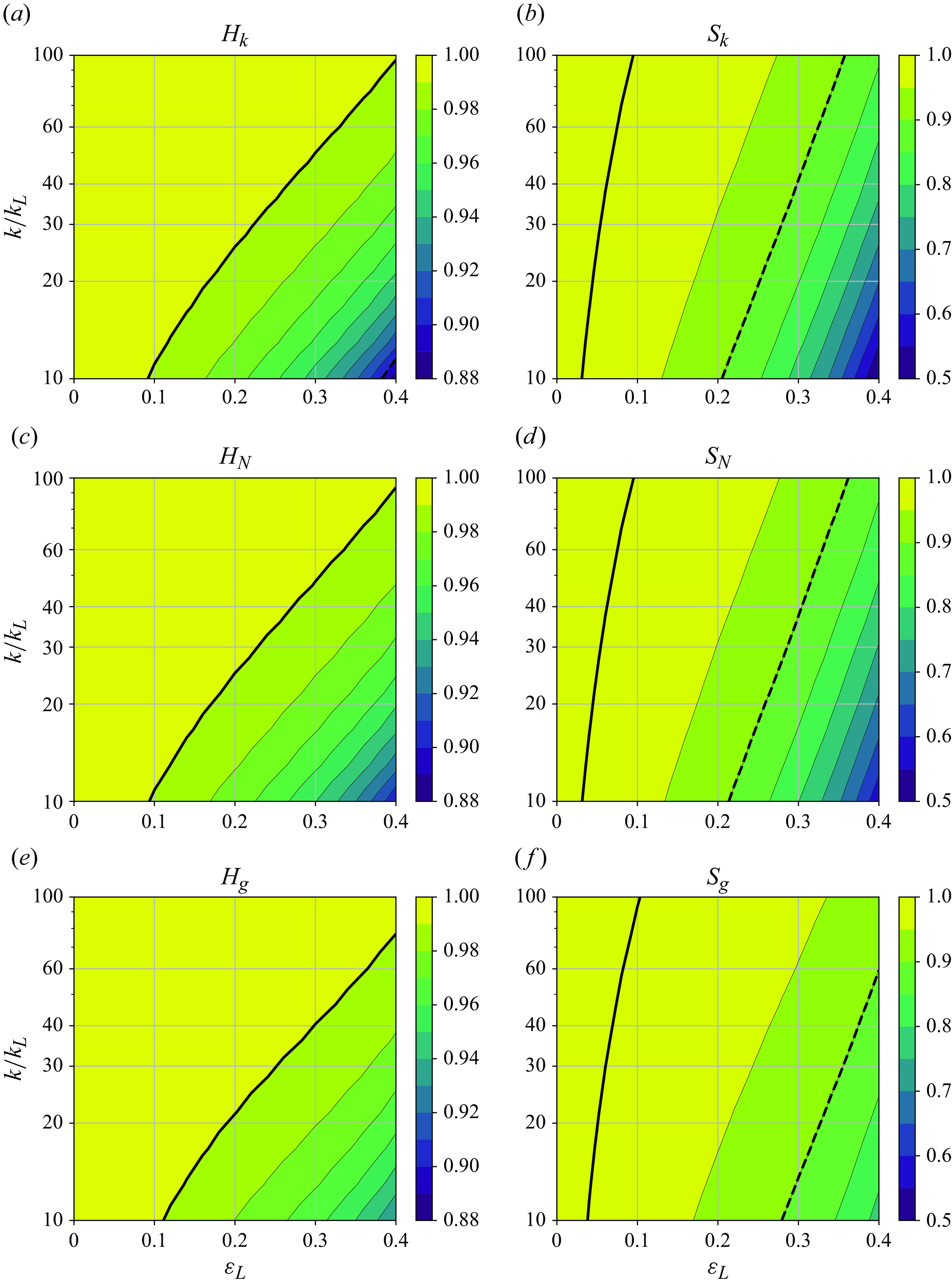
Figure 11. Homogeneity (a), (c), (e) and stationarity (b), (d), (f) of the short-wave wavenumber (a), (b), action (c), (d) and effective gravity (e), (f) as a function of the long-wave steepness $\varepsilon _L$
and the wavenumber ratio
$\varepsilon _L$
and the wavenumber ratio $k/k_L$
, based on the numerical solutions of the full wave crest and action conservation equations. Note that the colour ranges are different than those in figure 6.
$k/k_L$
, based on the numerical solutions of the full wave crest and action conservation equations. Note that the colour ranges are different than those in figure 6.
As the numerical solutions are for the nonlinear wave action and crest conservation equations, it is important to re-evaluate the homogeneity and stationarity requirements for the wave action conservation to remain valid. Figure 11 shows the homogeneities and stationarities of the short-wave wavenumber, action and effective gravity as functions of the long-wave steepness $\varepsilon _L$
and the wavenumber ratio
$\varepsilon _L$
and the wavenumber ratio $k/k_L$
, based on the numerical simulations. Although homogeneity is slightly lower (
$k/k_L$
, based on the numerical simulations. Although homogeneity is slightly lower ( $H_{k,N,g} \approx 0.92$
for
$H_{k,N,g} \approx 0.92$
for $k/k_L = 10$
and
$k/k_L = 10$
and $\varepsilon _L = 0.4$
) compared with the analytical solutions, the stationarity is significantly reduced. Following the same criteria for strong (
$\varepsilon _L = 0.4$
) compared with the analytical solutions, the stationarity is significantly reduced. Following the same criteria for strong ( $S_{k,N,g} \gt 0.99$
) and weak (
$S_{k,N,g} \gt 0.99$
) and weak ( $S_{k,N,g} \gt 0.9$
) stationarity as in § 3.4, the numerical solutions are only weakly stationary for
$S_{k,N,g} \gt 0.9$
) stationarity as in § 3.4, the numerical solutions are only weakly stationary for $\varepsilon _L \lt 0.21$
at
$\varepsilon _L \lt 0.21$
at $k/k_L = 10$
, and for
$k/k_L = 10$
, and for $\varepsilon _L \lt 0.36$
at
$\varepsilon _L \lt 0.36$
at $k/k_L = 100$
. This provides a quantitative guidance on when the short-wave action can be considered to be conserved in the presence of longer waves.
$k/k_L = 100$
. This provides a quantitative guidance on when the short-wave action can be considered to be conserved in the presence of longer waves.
4.3. Unsteady growth in Pereux et al. (Reference Peureux, Ardhuin and Guimarães2021)
The key result of Peureux et al. (Reference Peureux, Ardhuin and Guimarães2021) is that of unsteady steepening of short waves when a homogeneous field of short waves is forced by an infinite long-wave train. The steepening is driven by the progressive increase in the action of short waves (as opposed to their wavenumber), and is centred on the short-wave group that begins its journey in the trough of the long wave. This is because the unmodulated short waves that begin their journey in the trough first enter the convergence region before reaching the divergence region. Inversely, the short waves that begin around the crest of the long wave first enter the divergence region and will thus have their action and wavenumber decreased. We reproduce this behaviour in figure 12, which shows the evolution of the short-wave action, wavenumber and steepness modulation (here defined as the change of a quantity relative to its initial value). The long waves have $\varepsilon _L = 0.1$
and
$\varepsilon _L = 0.1$
and $k_L = 1$
, and the short waves have
$k_L = 1$
, and the short waves have $k = 10$
. After 10 long-wave periods, the short-wave action is approximately doubled, consistent with Peureux et al. (Reference Peureux, Ardhuin and Guimarães2021). Another important property of this solution is that the short-wave group that experiences peak amplification (attenuation) are not locked-in to the long-wave crests (troughs), as they are in the prior steady solutions (Longuet-Higgins & Stewart Reference Longuet-Higgins and Stewart1960; Longuet-Higgins Reference Longuet-Higgins1987; Zhang & Melville Reference Zhang and Melville1990).
$k = 10$
. After 10 long-wave periods, the short-wave action is approximately doubled, consistent with Peureux et al. (Reference Peureux, Ardhuin and Guimarães2021). Another important property of this solution is that the short-wave group that experiences peak amplification (attenuation) are not locked-in to the long-wave crests (troughs), as they are in the prior steady solutions (Longuet-Higgins & Stewart Reference Longuet-Higgins and Stewart1960; Longuet-Higgins Reference Longuet-Higgins1987; Zhang & Melville Reference Zhang and Melville1990).

Figure 12. Changes in the short-wave action (a), wavenumber (b) and steepness (c) relative to their initial values as functions of initial long-wave phase and time. Here, $k_L = 1$
,
$k_L = 1$
, $k = 10$
,
$k = 10$
, $\varepsilon _L = 0.1$
. The black contour follows the value of 1, which corresponds to no change from the initial values.
$\varepsilon _L = 0.1$
. The black contour follows the value of 1, which corresponds to no change from the initial values.
Why does this unsteady growth of short-wave action occur? Peureux et al. (Reference Peureux, Ardhuin and Guimarães2021) explain that the change in advection velocity due to the modulation of the short-wave group speed yields an additional amplification of the short-wave action. That is, the inhomogeneity term $N \partial C_g / \partial x$
is responsible for the instability. However, the instability only occurs if the short waves are initialised as a uniform field. If they are initialised instead as a periodic function of the long-wave phase such that their wavenumber (and optionally, action) is higher on the crests and lower in the troughs, akin to the prior steady solutions, the instability vanishes and the short-wave modulation pattern locks-in to the long-wave crests.
$N \partial C_g / \partial x$
is responsible for the instability. However, the instability only occurs if the short waves are initialised as a uniform field. If they are initialised instead as a periodic function of the long-wave phase such that their wavenumber (and optionally, action) is higher on the crests and lower in the troughs, akin to the prior steady solutions, the instability vanishes and the short-wave modulation pattern locks-in to the long-wave crests.
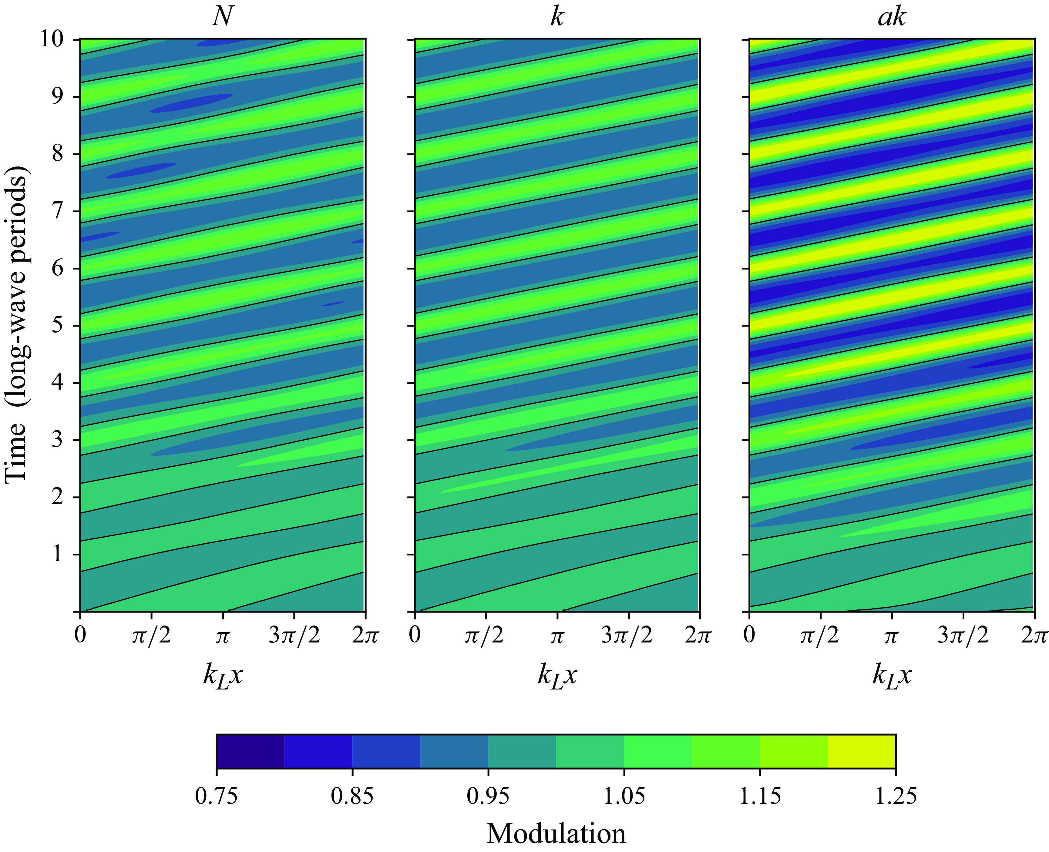
Figure 13. Same as figure 12 but with a linear ramp applied to $a_L$
during the initial five long-wave periods. Notice the change in the colour range.
$a_L$
during the initial five long-wave periods. Notice the change in the colour range.
Why is it, then, that the solution for short-wave modulation is not only quantitatively, but also qualitatively, different depending on the short-wave initial conditions? It may at first seem that there is something special about the uniform initial conditions that makes its solutions grow unsteadily and indefinitely. Peureux et al. (Reference Peureux, Ardhuin and Guimarães2021) described this scenario as ‘…the sudden appearance of a long-wave perturbation in the middle of a homogeneous short wave field’. However, it is not obvious whether such a scenario is common as waves tend to disperse into groups, and the time scales of incoming swell fronts are much longer than those of short-wave generation by wind. Exceptional situations with such a sudden onset of swell may occur around complex coastlines or in shadows behind islands, where wind-generated ripples may propagate from an otherwise calm sea state into the path of a crossing swell. Within the limits of the modulation theory used here, such short waves could quickly steepen and break.
To test whether the sudden onset of long-wave forcing causes the unsteady growth, we repeat the numerical simulation of figure 12, except for a linear ramp applied to $a_L$
(and consequently, the other long-wave properties including the orbital velocities and the local steepness) for the first five periods:
$a_L$
(and consequently, the other long-wave properties including the orbital velocities and the local steepness) for the first five periods: $a_L(t) = min(a_L, a_L t / (5 T_L ))$
, where
$a_L(t) = min(a_L, a_L t / (5 T_L ))$
, where $T_L$
is the long-wave period. This result is shown in figure 13. Note that the linear ramp is strictly a numerical modelling technique to test the sensitivity of the solution to the sudden forcing at the beginning of the simulation, and is not intended to represent a physical process. The key distinction that arises with the introduction of the ramp is that the modulation pattern of short waves is now locked-in to the long-wave crests, and their indefinite steepening vanishes. The stabilisation effect of the long-wave ramp is more readily assessed in figure 14, which shows the maximum short-wave steepness modulation as a function of time over 30 long-wave periods, for the infinite long-wave train case and the case of applying a linear ramp. Comparing the wave action propagation (
$T_L$
is the long-wave period. This result is shown in figure 13. Note that the linear ramp is strictly a numerical modelling technique to test the sensitivity of the solution to the sudden forcing at the beginning of the simulation, and is not intended to represent a physical process. The key distinction that arises with the introduction of the ramp is that the modulation pattern of short waves is now locked-in to the long-wave crests, and their indefinite steepening vanishes. The stabilisation effect of the long-wave ramp is more readily assessed in figure 14, which shows the maximum short-wave steepness modulation as a function of time over 30 long-wave periods, for the infinite long-wave train case and the case of applying a linear ramp. Comparing the wave action propagation ( $C_g \partial N / \partial x$
) and inhomogeneity (
$C_g \partial N / \partial x$
) and inhomogeneity ( $N \partial C_g / \partial x$
) tendencies reveals that, after only one long-wave period, the propagation and inhomogeneity tendencies are unbalanced and amplify the steepening of short waves (figure 15). Peureux et al. (Reference Peureux, Ardhuin and Guimarães2021) correctly pointed out that the unsteady growth of short-wave steepness occurs due to the resonance of the inhomogeneity tendency with the short-wave action perturbation. However, in the case of a gentle ramp-up of the long-wave forcing, the propagation and inhomogeneity tendencies balance each other and allow the short-wave steepening to lock-in to the long-wave crests.
$N \partial C_g / \partial x$
) tendencies reveals that, after only one long-wave period, the propagation and inhomogeneity tendencies are unbalanced and amplify the steepening of short waves (figure 15). Peureux et al. (Reference Peureux, Ardhuin and Guimarães2021) correctly pointed out that the unsteady growth of short-wave steepness occurs due to the resonance of the inhomogeneity tendency with the short-wave action perturbation. However, in the case of a gentle ramp-up of the long-wave forcing, the propagation and inhomogeneity tendencies balance each other and allow the short-wave steepening to lock-in to the long-wave crests.
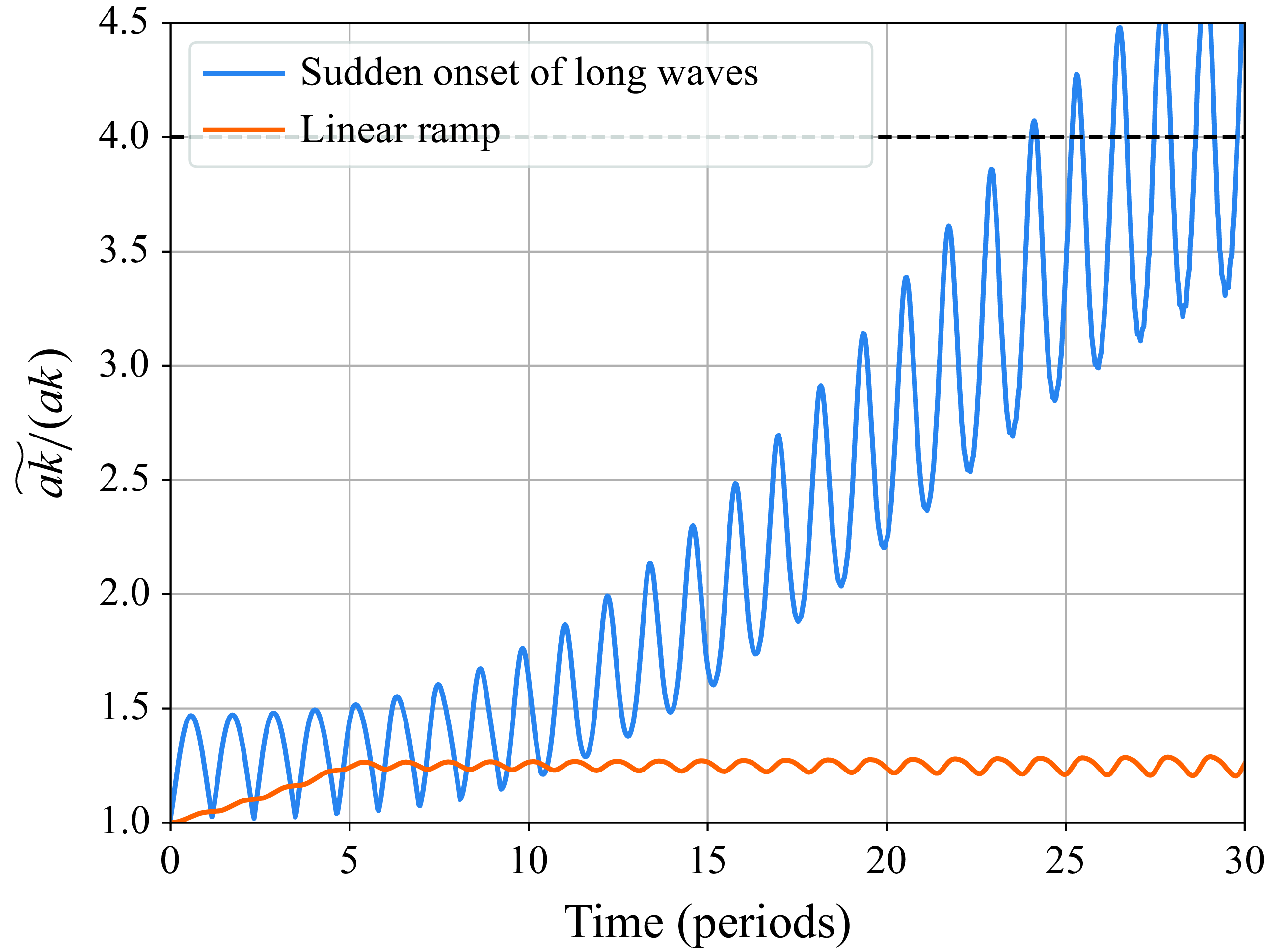
Figure 14. Maximum short-wave steepness modulation as a function of time in case of infinite long-wave train case (blue) and the same case but with a linear ramp during the initial five long-wave periods (orange). The dashed black line corresponds to the short-wave steepness of 0.4 at which most waves are expected to break.
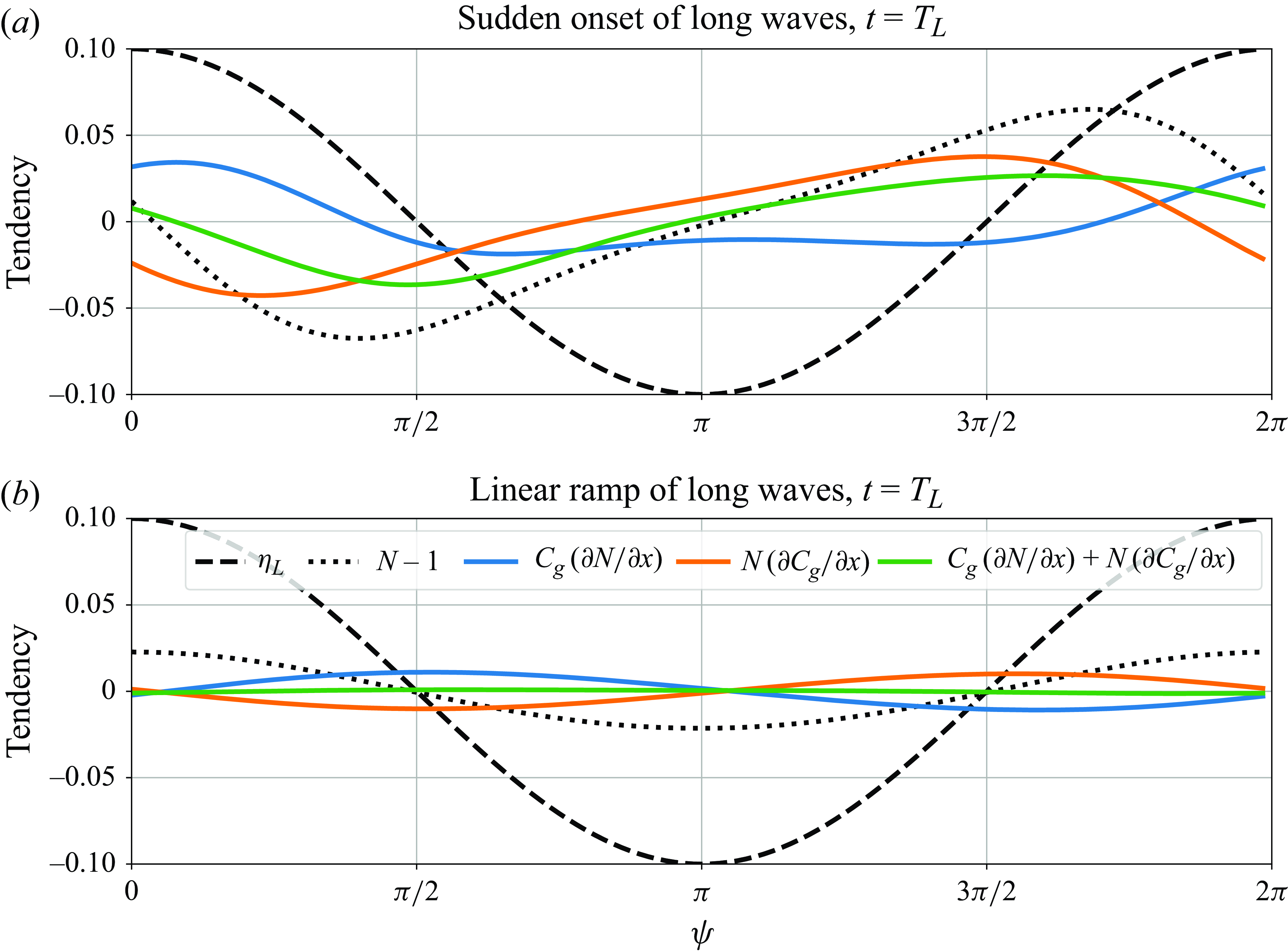
Figure 15. Propagation ( $C_g {\partial N}/{\partial x}$
) (blue) and inhomogeneity (
$C_g {\partial N}/{\partial x}$
) (blue) and inhomogeneity ( $N {\partial C_g}/{\partial x}$
) (orange) tendencies and their sum (green) for the short-wave action after one long-wave period, in the case of (a) an infinitely long-wave train and (b) a linear ramp of long-wave amplitude. Dashed line is the long-wave elevation and the dotted line is the short-wave action modulation minus 1.
$N {\partial C_g}/{\partial x}$
) (orange) tendencies and their sum (green) for the short-wave action after one long-wave period, in the case of (a) an infinitely long-wave train and (b) a linear ramp of long-wave amplitude. Dashed line is the long-wave elevation and the dotted line is the short-wave action modulation minus 1.
4.4. Modulation by long waves of varying amplitude
We now proceed to examine the numerical solutions of short-wave modulation by long waves whose amplitude varies with time. The amplitude variation aims to mimic the behaviour of long-wave groups, a phenomenon that is ubiquitous in the ocean due to the dispersive nature of surface gravity waves, as well as due to the fact that wind-generated waves evolve to have broad-banded spectra. For simplicity of implementation and interpretation, the wave group here is simulated as a non-dispersive train of long waves whose amplitude scales with $\sin [\pi t / (n T_L)]$
, where
$\sin [\pi t / (n T_L)]$
, where $n$
is the number of long waves in the group. The elevation of the long waves thus gradually ramps up from rest to
$n$
is the number of long waves in the group. The elevation of the long waves thus gradually ramps up from rest to $a_L$
at
$a_L$
at $t = n T_L / 2$
, after which it gradually decreases toward zero. In this simulation,
$t = n T_L / 2$
, after which it gradually decreases toward zero. In this simulation, $k/k_L = 10$
and
$k/k_L = 10$
and $\varepsilon _L = 0.1$
as in the previous two simulations. The modulations of short-wave wavenumber, amplitude and steepness in response to such long-wave group is shown in figure 16. Like in the case of a linear ramp, the modulation pattern here is locked in to the long-wave crest and peaks at approximately 1.2 for short-wave steepness of 0.1. After the peak of the long-wave group passes, the short-wave modulation recedes back toward the resting state.
$\varepsilon _L = 0.1$
as in the previous two simulations. The modulations of short-wave wavenumber, amplitude and steepness in response to such long-wave group is shown in figure 16. Like in the case of a linear ramp, the modulation pattern here is locked in to the long-wave crest and peaks at approximately 1.2 for short-wave steepness of 0.1. After the peak of the long-wave group passes, the short-wave modulation recedes back toward the resting state.
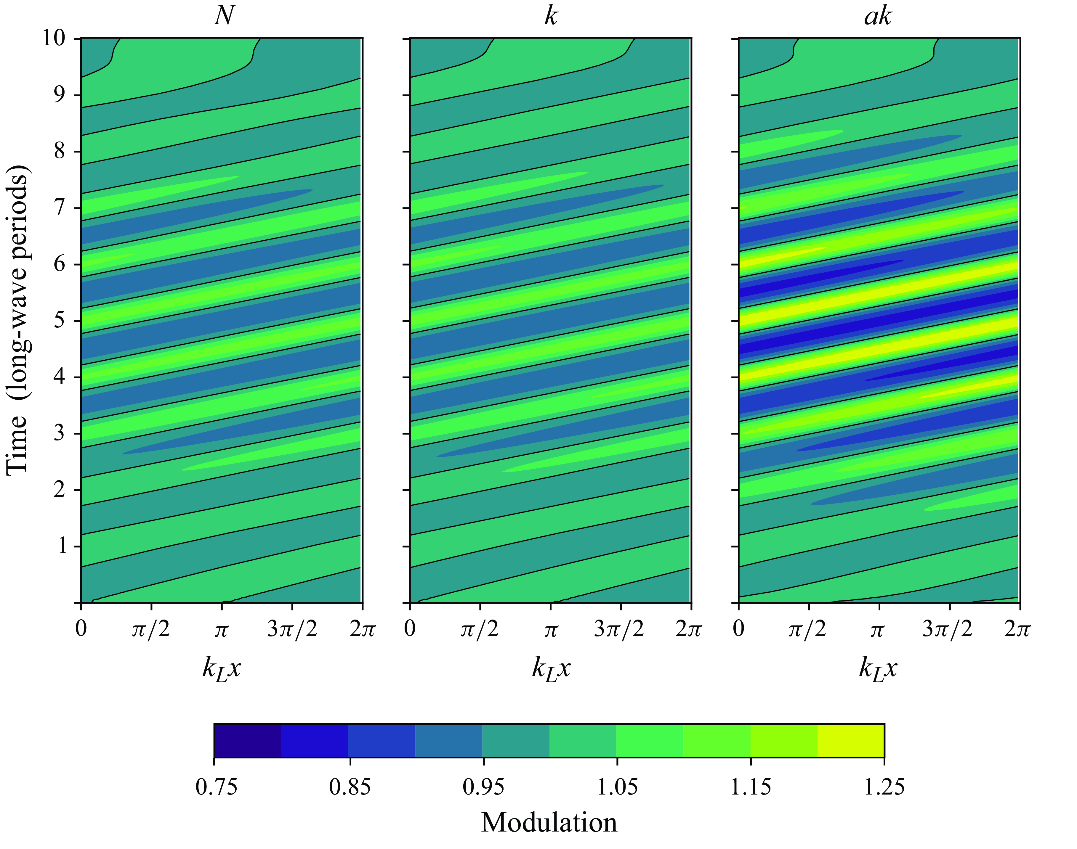
Figure 16. Same as figure 12 but for a long-wave group, causing the long-wave amplitude to gradually increase and peak at $a_L = 0.1$
after five long-wave periods, and then conversely decay back to a calm sea state.
$a_L = 0.1$
after five long-wave periods, and then conversely decay back to a calm sea state.
5. Discussion
The solutions presented here, analytical and numerical alike, are valid only for certain scales of short and long waves. Specifically, the wave action conservation equation, introduced by Bretherton & Garrett (Reference Bretherton and Garrett1968), requires that the ambient velocity is slowly varying on the time scales of short waves, i.e. $|\partial U / \partial x| \ll k |U|$
and
$|\partial U / \partial x| \ll k |U|$
and $|\partial U / \partial t| \ll \sigma |U|$
. This implies
$|\partial U / \partial t| \ll \sigma |U|$
. This implies $k_L \ll k$
and
$k_L \ll k$
and $\sigma _L \ll \sigma$
, respectively. The same requirement is imposed on the properties of short waves, including wavenumber, amplitude and effective gravity. Another requirement is for the short waves to remain linear, which implies
$\sigma _L \ll \sigma$
, respectively. The same requirement is imposed on the properties of short waves, including wavenumber, amplitude and effective gravity. Another requirement is for the short waves to remain linear, which implies $a k \ll 1$
. These requirements have been evaluated for the solutions presented here by quantifying the homogeneity and stationarity of each relevant property of the flow in § 3.4. Furthermore, the short waves examined here do not include the effects of surface tension (gravity-capillary waves) or intermediate or shallow water, although the solutions can be extended to those conditions, as Phillips (Reference Phillips1981) did, for example. Within these limits, the crest-action conservation equations provide an elegant and simple framework to study the hydrodynamic modulation of short waves by longer waves. This approach, of course, isolates this particular process from other dominant modulation and nonlinear transfer processes, such as wave growth by wind, wave dissipation and aerodynamic sheltering by the longer waves, that are otherwise present in most measurements (e.g. Plant Reference Plant1986; Laxague et al. Reference Laxague, Curcic, Bjorkqvist and Haus2017). An alternative approach using a fully nonlinear velocity potential flow solver that allows for two-way interaction between short and long waves would provide additional insight into the modulation of the long waves by the short waves.
$a k \ll 1$
. These requirements have been evaluated for the solutions presented here by quantifying the homogeneity and stationarity of each relevant property of the flow in § 3.4. Furthermore, the short waves examined here do not include the effects of surface tension (gravity-capillary waves) or intermediate or shallow water, although the solutions can be extended to those conditions, as Phillips (Reference Phillips1981) did, for example. Within these limits, the crest-action conservation equations provide an elegant and simple framework to study the hydrodynamic modulation of short waves by longer waves. This approach, of course, isolates this particular process from other dominant modulation and nonlinear transfer processes, such as wave growth by wind, wave dissipation and aerodynamic sheltering by the longer waves, that are otherwise present in most measurements (e.g. Plant Reference Plant1986; Laxague et al. Reference Laxague, Curcic, Bjorkqvist and Haus2017). An alternative approach using a fully nonlinear velocity potential flow solver that allows for two-way interaction between short and long waves would provide additional insight into the modulation of the long waves by the short waves.
Although in this paper we only explored the solutions for $k_L = 1$
and
$k_L = 1$
and $k=10$
the results are not sensitive to different values of
$k=10$
the results are not sensitive to different values of $k_L$
, provided the same long-wave steepness
$k_L$
, provided the same long-wave steepness $\varepsilon _L = a_L k_L$
. Numerical simulations with
$\varepsilon _L = a_L k_L$
. Numerical simulations with $k/k_L = 10$
and
$k/k_L = 10$
and $k/k_L = 100$
show little sensitivity to the ratio
$k/k_L = 100$
show little sensitivity to the ratio $k/k_L$
(not shown), consistent with the results of Longuet-Higgins (Reference Longuet-Higgins1987). Specifically, the short-wave steepness modulation is 1% larger at
$k/k_L$
(not shown), consistent with the results of Longuet-Higgins (Reference Longuet-Higgins1987). Specifically, the short-wave steepness modulation is 1% larger at $\varepsilon _L = 0.27$
for
$\varepsilon _L = 0.27$
for $k/k_L = 10$
compared with
$k/k_L = 10$
compared with $k/k_L = 100$
, and 4 % larger at
$k/k_L = 100$
, and 4 % larger at $\varepsilon _L = 0.4$
. This suggests that as long as
$\varepsilon _L = 0.4$
. This suggests that as long as $k/k_L \gg 1$
, the modulation amplitude is largely independent of the ratio
$k/k_L \gg 1$
, the modulation amplitude is largely independent of the ratio $k/k_L$
. These results can be reproduced with the companion numerical model. Note, however, according to § 3.4, that the wave action conservation requirements are more easily satisfied for larger
$k/k_L$
. These results can be reproduced with the companion numerical model. Note, however, according to § 3.4, that the wave action conservation requirements are more easily satisfied for larger $k/k_L$
. Also not considered here are the short-wave trains that are oblique to the longer waves, which is relatively straightforward to include (Peureux et al. Reference Peureux, Ardhuin and Guimarães2021).
$k/k_L$
. Also not considered here are the short-wave trains that are oblique to the longer waves, which is relatively straightforward to include (Peureux et al. Reference Peureux, Ardhuin and Guimarães2021).
Despite several studies that provided qualitatively similar steady solutions for the short-wave modulation by long waves (Longuet-Higgins & Stewart Reference Longuet-Higgins and Stewart1960; Phillips Reference Phillips1981; Longuet-Higgins Reference Longuet-Higgins1987; Henyey et al. Reference Henyey, Creamer, Dysthe, Schult and Wright1988; Zhang & Melville Reference Zhang and Melville1990), it was not obvious from the governing prognostic equations that the steady solutions should exist generally. Peureux et al. (Reference Peureux, Ardhuin and Guimarães2021) examined this problem numerically and found that the solutions are stable only if the short-wave field is initialised from a prior steady solution of the form of that from Longuet-Higgins & Stewart (Reference Longuet-Higgins and Stewart1960). If the short-wave field is instead initialised from a uniform field, they found that the short-wave amplitude, and thus steepness as well, grow unsteadily and indefinitely. Here, we demonstrate that the unsteady steepening of short waves only occurs in the case of a sudden appearance of long waves, where the velocity fields induced by the long waves act in their full capacity on the short waves that have not yet had time to lock-in to the long-wave crests. In such a scenario, sudden forcing on short waves causes the modulation pattern to detach itself from the long-wave crests and to propagate at the short-wave group speed. When this occurs, the modulated short waves are no longer in a stabilising resonance with the surface convergence and divergence induced by the long-wave orbital velocity, and each long-wave passage further destabilises the short-wave field, causing it to steepen indefinitely.
Another important consideration of the hydrodynamic modulation process is whether it should be accounted for in phase-averaged spectral wave models (WAMDI Group 1988; Tolman Reference Tolman1991; Donelan et al. Reference Donelan, Curcic, Chen and Magnusson2012) used for global and regional wave forecasting. Second-order wave spectra have historically been provided by some wave models due to their importance for understanding radar altimetry data, however, only in a diagnostic capacity (e.g. Janssen Reference Janssen2009). The framework by Janssen (Reference Janssen2009), based on the Hamiltonian and the action series expansion by Zakharov (Reference Zakharov1968), is an alternative and more general approach to nonlinear wave evolution than the one described here. Currently, most spectral wave models used for research or forecasting do not consider the preferential steepening of short waves in the context of their dispersion properties or the wind input via the short-wave phase speed. Some dissipation source functions use the cumulative mean squared slope to quantify preferential dissipation of short waves due to this effect (Donelan et al. Reference Donelan, Curcic, Chen and Magnusson2012; Romero Reference Romero2019). In the early days of spectral wave modelling, Willebrand (Reference Willebrand1975) examined the effect of a wave spectrum on the short-wave group velocity and found the modulation effect to be up to several per cent. For a practical implementation, this would incur an additional loop over all frequencies longer than the considered short-wave frequency. It was thus not deemed practical to include this effect in wave models at the time. However, with the recent advances in computing power, machine learning for acceleration of complex functions and phase-resolved modelling of short waves, considering the effect of wave modulation beyond the simple cumulative mean squared slope deserves re-examination.
6. Conclusions
In this paper we revisited the problem of short-wave modulation by long waves from a wave action conservation perspective. Using the linearised wave crest and action conservation equations coupled with nonlinear solutions for the effective gravity, we derived steady, nonlinear, analytical solutions for the modulation of short-wave wavenumber, amplitude, steepness, intrinsic frequency and phase speed. The latter two were previously examined in the context of resonant interactions (Longuet-Higgins Reference Longuet-Higgins1962; Longuet-Higgins & Phillips Reference Longuet-Higgins and Phillips1962), a modulation process distinct from the one discussed here. Both effects, however, may be important for correctly calculating the wind input into short waves, which is proportional to the wind speed relative to the wave celerity. The approximate steady solutions yield higher wavenumber and amplitude modulation than that of Longuet-Higgins & Stewart (Reference Longuet-Higgins and Stewart1960), and somewhat lower than the numerical solutions of Longuet-Higgins (Reference Longuet-Higgins1987) and Zhang & Melville (Reference Zhang and Melville1990). This is mainly due to the analytical solution requiring the crest and action conservation equations to be linearised, and the nonlinearity arising due to the evaluation of short waves on the surface of the long wave (as opposed to the mean water level) and due to nonlinear effective gravity. In the steady solutions, the short-wave steepness modulation is dominated by the wavenumber modulation (5/8), followed by the wave action modulation (1/4) and is least affected by the effective-gravity modulation (1/8). The homogeneity and stationarity criteria for wave action conservation are evaluated for both the analytical and numerical solutions. The stationarity is a stronger criterion than homogeneity, and is found to be strongly satisfied ( ${\gt}99\, \%$
stationary) for very gently sloped waves and weakly satisfied (
${\gt}99\, \%$
stationary) for very gently sloped waves and weakly satisfied ( ${\gt}90\, \%$
stationary) for steeper waves.
${\gt}90\, \%$
stationary) for steeper waves.
The numerical solutions of the full wave crest and action conservation equations are consistent with the analytical solutions for $\varepsilon _L \lesssim 0.2$
, and are similar in magnitude to the numerical solutions of Longuet-Higgins (Reference Longuet-Higgins1987) and Zhang & Melville (Reference Zhang and Melville1990). The simulations also reveal that the unsteady growth of the short-wave steepness reported by Peureux et al. (Reference Peureux, Ardhuin and Guimarães2021) is due to the sudden appearance of long waves in a homogeneous short-wave field, a scenario that is unlikely to be common in the open ocean. A more likely condition, such as that of long-wave groups, is only mildly destabilising for the short waves. These results suggest that, for the long-wave steepness
$\varepsilon _L \lesssim 0.2$
, and are similar in magnitude to the numerical solutions of Longuet-Higgins (Reference Longuet-Higgins1987) and Zhang & Melville (Reference Zhang and Melville1990). The simulations also reveal that the unsteady growth of the short-wave steepness reported by Peureux et al. (Reference Peureux, Ardhuin and Guimarães2021) is due to the sudden appearance of long waves in a homogeneous short-wave field, a scenario that is unlikely to be common in the open ocean. A more likely condition, such as that of long-wave groups, is only mildly destabilising for the short waves. These results suggest that, for the long-wave steepness $\varepsilon _L \lesssim 0.2$
, the analytical steady solutions presented here are sufficient to describe the modulation of short waves by long waves. For moderately steep long waves (
$\varepsilon _L \lesssim 0.2$
, the analytical steady solutions presented here are sufficient to describe the modulation of short waves by long waves. For moderately steep long waves ( $0.2 \lesssim \varepsilon _L \lesssim 0.3$
), numerical solutions of nonlinearised crest and action conservation equations are necessary to properly capture the short-wave steepness modulation. For steeper long waves (
$0.2 \lesssim \varepsilon _L \lesssim 0.3$
), numerical solutions of nonlinearised crest and action conservation equations are necessary to properly capture the short-wave steepness modulation. For steeper long waves ( $\varepsilon _L \gtrsim 0.3$
), the short-wave properties can no longer be considered stationary (Bretherton & Garrett Reference Bretherton and Garrett1968); the wave action conservation equation is thus not valid in this context. It may be worthwhile to revisit a more systematic inclusion of the hydrodynamic modulation effects in phase-averaged spectral wave models, beyond the simple cumulative mean squared slope for wave dissipation, but also for modulating the dispersion and wind input into short waves.
$\varepsilon _L \gtrsim 0.3$
), the short-wave properties can no longer be considered stationary (Bretherton & Garrett Reference Bretherton and Garrett1968); the wave action conservation equation is thus not valid in this context. It may be worthwhile to revisit a more systematic inclusion of the hydrodynamic modulation effects in phase-averaged spectral wave models, beyond the simple cumulative mean squared slope for wave dissipation, but also for modulating the dispersion and wind input into short waves.
Acknowledgements
I am thankful to N. Laxague, F. Ardhuin, N. Pizzo, and P. Tan for fruitful discussions. I also thank the three anonymous reviewers for their expertise that helped improve this paper.
Funding
M.C. was partly supported by the National Science Foundation grant AGS-1745384, Transatlantic Research Partnership by the French Embassy in the United States and the FACE Foundation, and the Office of Naval Research grants N000142012102 (Coastal Land Air-Sea Interaction DRI) and N000142412598 (in collaboration with SASCWATCH: Study on Air-Sea Coupling with WAves, Turbulence, and Clouds at High winds MURI).
Declaration of interests
The author reports no conflict of interest.
Data availability statement
The code to run the numerical simulations and generate the figures in this paper is available at https://github.com/wavesgroup/wave-modulation-paper. The numerical model is available as a standalone Python package at https://github.com/wavesgroup/2wave. A Python implementation of the Steady Surface Gravity Wave (SSGW) package by Clamond & Dutykh (Reference Clamond and Dutykh2018) is available at https://github.com/wavesgroup/ssgw.
Appendix A. Derivation of the governing equations
Here, we derive the governing equations for the short waves (2.1)–(2.3) and discuss their asymptotic consistency.
A.1. Wave dispersion
An irrotational flow has a velocity potential such that the continuity can be expressed as
 \begin{equation} \nabla ^2 \phi = 0. \end{equation}
Boundary conditions that allow solving for $\phi$
are the dynamic and kinematic free surface boundary conditions, respectively,
$\phi$
are the dynamic and kinematic free surface boundary conditions, respectively,
 \begin{equation} \frac {\partial \phi }{\partial t} + \frac {1}{2} (\nabla {\phi })^2 + gz = 0 \quad \text{at} \quad z = \eta (x,t), \end{equation}
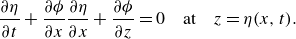 \begin{equation} \frac {\partial \eta }{\partial t} + \frac {\partial \phi }{\partial x} \frac {\partial \eta }{\partial x} + \frac {\partial \phi }{\partial z} = 0 \quad \text{at} \quad z = \eta (x,t). \end{equation}
Also required is the bottom boundary condition
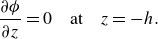 \begin{equation} \frac {\partial \phi }{\partial z} = 0 \quad \text{at} \quad z = -h. \end{equation}
In the Stokes (Reference Stokes1847) perturbation approach, the velocity potential and elevation are expanded in a power series of the wave steepness $\varepsilon = ak$
as
$\varepsilon = ak$
as
 \begin{equation} \phi = \sum _{n=1}^{\infty } \varepsilon ^n \phi _n, \end{equation}
 \begin{equation} \eta = \sum _{n=1}^{\infty } \varepsilon ^n \eta _n. \end{equation}
The power series expansion requires $\varepsilon \ll 1$
. The velocity potential and elevation series are truncated at the desired order and inserted into the dynamic free surface boundary condition (A2). Up to the third order, the solutions for the velocity potential and the corresponding velocity components are (2.7)–( 2.9), and the surface elevation is (3.11). Evaluating these quantities to higher orders in
$\varepsilon \ll 1$
. The velocity potential and elevation series are truncated at the desired order and inserted into the dynamic free surface boundary condition (A2). Up to the third order, the solutions for the velocity potential and the corresponding velocity components are (2.7)–( 2.9), and the surface elevation is (3.11). Evaluating these quantities to higher orders in $\varepsilon$
is possible at the expense of higher complexity and with diminishing returns in accuracy.
$\varepsilon$
is possible at the expense of higher complexity and with diminishing returns in accuracy.
Combining the solutions for the potential and the surface elevation with the kinematic free surface boundary condition (A3) yields the dispersion relation, which in the linear case and in deep water is (2.1). At the third order in $\varepsilon$
, the frequency begins to depend on the wave steepness
$\varepsilon$
, the frequency begins to depend on the wave steepness $\varepsilon$
as well
$\varepsilon$
as well
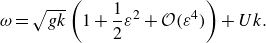 \begin{equation} \omega = \sqrt {g k} \left (1 + \frac {1}{2} \varepsilon ^2 + {\mathcal{O}}(\varepsilon ^4)\right ) + U k. \end{equation}
In this paper we constrain the analysis framework to the linear case for short waves, as this permits the analytical solutions in § 3. The Doppler shift by the ambient velocity $U$
is unaffected by the nonlinear effects in the solution.
$U$
is unaffected by the nonlinear effects in the solution.
A.2. Conservation of wave crests
A system with a well-defined phase function $\psi (x,t)$
also has the wavenumber and frequency defined as its gradients with respect to space and time, respectively,
$\psi (x,t)$
also has the wavenumber and frequency defined as its gradients with respect to space and time, respectively,
 \begin{equation} k = \frac {\partial \psi }{\partial x}, \end{equation}
 \begin{equation} \omega = - \frac {\partial \psi }{\partial t}, \end{equation}
implying $\psi = kx - \omega t$
. Differentiating (A8)–(A9) with respect to time and space, respectively, and then eliminating
$\psi = kx - \omega t$
. Differentiating (A8)–(A9) with respect to time and space, respectively, and then eliminating $\psi$
yields
$\psi$
yields
 \begin{equation} \frac {\partial k}{\partial t} + \frac {\partial \omega }{\partial x} = 0, \end{equation}
which is the crest conservation equation (2.2). That this is the wavenumber conservation equation with the group speed as the transport velocity can be recognised by writing
 \begin{equation} \frac {\partial k}{\partial t} + \frac {\partial \omega }{\partial k} \frac {\partial k}{\partial x} = 0. \end{equation}
This conservation equation is valid regardless of the order of nonlinearity considered, as long as $\psi$
is well defined. Nonlinearity in terms of
$\psi$
is well defined. Nonlinearity in terms of $\varepsilon$
can, however, enter (A10) through nonlinear forms of
$\varepsilon$
can, however, enter (A10) through nonlinear forms of $\omega$
such as (A7).
$\omega$
such as (A7).
A.3. Conservation of wave action
The conservation of wave action (2.3) is most readily derived following the variational approach by Whitham (Reference Whitham1965). We begin with a statement that infinitesimal variations of a Lagrangian of a system over a spatial domain and time interval must vanish
 \begin{equation} \delta \iint L\, {\textrm d}x\,{\textrm d}t = 0. \end{equation}
Here, $L$
is the instantaneous Lagrangian density, a scalar quantity that corresponds to the difference between the kinetic and potential energy of the system
$L$
is the instantaneous Lagrangian density, a scalar quantity that corresponds to the difference between the kinetic and potential energy of the system
 \begin{equation} L = \int _{-h}^{\eta } \left [ \tfrac {1}{2} (\nabla {\phi })^2 + gz \right ] {\textrm d}z. \end{equation}
Luke (Reference Luke1967) showed that the equations for irrotational surface waves follow from the variational approach if the Lagrangian $L$
is defined instead as
$L$
is defined instead as
 \begin{equation} L = \int _{-h}^{\eta } \left [ \frac {\partial \phi }{\partial t} + \frac {1}{2} (\nabla {\phi })^2 + gz \right ] {\textrm d}z. \end{equation}
Equations (A13) and (A14) are equivalent in the sense that they both yield (A1), however, varying the latter is necessary to attain the correct boundary conditions (Whitham Reference Whitham1967). Notice that for water waves the instantaneous Lagrangian being zero is equivalent to the Bernoulli equation, which is also the dynamic free surface boundary condition.
Then, Whitham’s averaged variation principle is obtained by averaging the instantaneous Lagrangian $L$
over one wave period
$L$
over one wave period
 \begin{equation} {\mathcal{L}} = \frac {1}{2\pi } \int _0^{2\pi } L\ {\textrm d}\psi, \end{equation}
where ${\mathcal{L}}$
is the averaged Lagrangian density. The averaged variational principle then states
${\mathcal{L}}$
is the averaged Lagrangian density. The averaged variational principle then states
 \begin{equation} \delta \iint {\mathcal{L}}\, {\textrm d}x\,{\textrm d}t = 0. \end{equation}
The averaged Lagrangian for water waves is obtained by integrating (A14) over depth, and then averaging over the phase (A15). In the deep-water limit, it is
 \begin{equation} {\mathcal{L}} = \frac {1}{4} \left ( 1 - \frac {\omega ^2}{gk} \right ) g a^2 + {\mathcal{O}}(\varepsilon ^4), \end{equation}
which, after recognising the wave energy $E = {1}/{2} g a^2$
, yields
$E = {1}/{2} g a^2$
, yields
 \begin{equation} {\mathcal{L}} = \frac {1}{2} \left ( 1 - \frac {\omega ^2}{gk} \right ) E + {\mathcal{O}}(\varepsilon ^4). \end{equation}
Whitham’s conservation equations for water waves are
 \begin{equation} \frac {\partial {\mathcal{L}}}{\partial a} = 0, \end{equation}
 \begin{equation} \frac {\partial }{\partial t} \left (\frac {\partial {\mathcal{L}}}{\partial \omega }\right ) - \frac {\partial }{\partial x} \left (\frac {\partial {\mathcal{L}}}{\partial k}\right ) = 0. \end{equation}
Inserting (A18) into (A20) and defining
 \begin{equation} \frac {\partial {\mathcal{L}}}{\partial \omega } = \frac {E}{\sigma } \equiv N, \end{equation}
yields the conservation of wave action
 \begin{equation} \frac {\partial }{\partial t} \big[ N + {\mathcal{O}}(\varepsilon ^4) \big] + \frac {\partial }{\partial x} \big[ (C_g + {\mathcal{O}}(\varepsilon ^2)) (N + {\mathcal{O}}(\varepsilon ^4)) \big] = 0. \end{equation}
Due to the ${\mathcal{O}}(\varepsilon ^2)$
correction to the group speed, the overall truncation error for the wave action balance is
${\mathcal{O}}(\varepsilon ^2)$
correction to the group speed, the overall truncation error for the wave action balance is ${\mathcal{O}}(\varepsilon ^2)$
as well
${\mathcal{O}}(\varepsilon ^2)$
as well
 \begin{equation} \frac {\partial N}{\partial t} + \frac {\partial (C_g N)}{\partial x} = {\mathcal{O}}(\varepsilon ^2), \end{equation}
which was introduced as a governing equation in § 2. Although the truncation error of ${\mathcal{O}}(\varepsilon ^2)$
arising from
${\mathcal{O}}(\varepsilon ^2)$
arising from $C_g$
seems to have been omitted in the original derivation by Whitham (Reference Whitham1967), it appeared correctly later in Whitham (Reference Whitham1974). An important nuance about applying the nonlinear dispersion here is that the secondary (wave-induced) mean flow and set-up effects can be ignored in the deep-water limit; this is discussed by Whitham (Reference Whitham1974). The terms proportional to
$C_g$
seems to have been omitted in the original derivation by Whitham (Reference Whitham1967), it appeared correctly later in Whitham (Reference Whitham1974). An important nuance about applying the nonlinear dispersion here is that the secondary (wave-induced) mean flow and set-up effects can be ignored in the deep-water limit; this is discussed by Whitham (Reference Whitham1974). The terms proportional to $\varepsilon ^4$
do not appear in the averaged Lagrangian (A18) until the third-order Stokes waves are considered, for which the dispersion gains a
$\varepsilon ^4$
do not appear in the averaged Lagrangian (A18) until the third-order Stokes waves are considered, for which the dispersion gains a ${\mathcal{O}}(\varepsilon ^2)$
correction. In that case, the conserved quantity is
${\mathcal{O}}(\varepsilon ^2)$
correction. In that case, the conserved quantity is
 \begin{equation} \frac {\partial {\mathcal{L}}}{\partial \omega } = \frac {E}{\sigma } \left(1 + \frac {1}{2} \varepsilon ^2 \right), \end{equation}
and the group speed gains a nonlinear factor in $\varepsilon ^2$
as well. Equation (A23), then, maintains the same form, but with the truncation error of
$\varepsilon ^2$
as well. Equation (A23), then, maintains the same form, but with the truncation error of ${\mathcal{O}}(\varepsilon ^4)$
. This derivation, as well as the averaged Lagrangian principle applied to the wave-induced mean flow over arbitrary water depths, is detailed at greater length by Whitham (Reference Whitham1967).
${\mathcal{O}}(\varepsilon ^4)$
. This derivation, as well as the averaged Lagrangian principle applied to the wave-induced mean flow over arbitrary water depths, is detailed at greater length by Whitham (Reference Whitham1967).
Table 2. Asymptotically consistent sets of dispersion and wave action relations for deep water and their respective truncation errors in terms of the wave steepness $\varepsilon$
, for the first three Stokes expansion orders.
$\varepsilon$
, for the first three Stokes expansion orders.

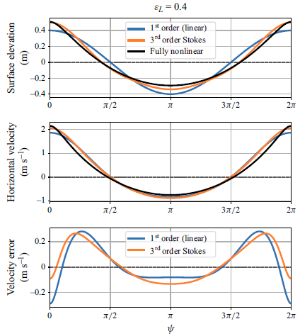
Figure 17. Surface elevation (top) and horizontal velocity (middle) for the linear wave (blue), the third-order Stokes wave (orange), and the fully nonlinear wave (black) with steepness of $\varepsilon _L = 0.4$
. The bottom panel shows the surface velocity error for the linear wave (blue) and the third-order Stokes wave (orange), relative to the fully nonlinear wave solution.
$\varepsilon _L = 0.4$
. The bottom panel shows the surface velocity error for the linear wave (blue) and the third-order Stokes wave (orange), relative to the fully nonlinear wave solution.
To consider the effect of slowly varying ambient currents, Bretherton & Garrett (Reference Bretherton and Garrett1968) carried out the same derivation except that they propagated the ambient current derivatives $\partial U / \partial t$
and
$\partial U / \partial t$
and $\partial U / \partial x$
through the averaged Lagrangian. To allow these derivatives to drop out of the averaging integral, the authors make an argument that the variation must be sufficiently small, no larger than
$\partial U / \partial x$
through the averaged Lagrangian. To allow these derivatives to drop out of the averaging integral, the authors make an argument that the variation must be sufficiently small, no larger than ${\mathcal{O}}{(1 / {\sigma}/{U}} {\partial U}/{\partial t})$
and
${\mathcal{O}}{(1 / {\sigma}/{U}} {\partial U}/{\partial t})$
and ${\mathcal{O}}({1}/{k/U} {\partial U}/{\partial x})$
, respectively. Taking into consideration the asymptotic limits in terms of the wave steepness
${\mathcal{O}}({1}/{k/U} {\partial U}/{\partial x})$
, respectively. Taking into consideration the asymptotic limits in terms of the wave steepness $\varepsilon$
as well as the variation of the ambient current, the wave action balance can be written as
$\varepsilon$
as well as the variation of the ambient current, the wave action balance can be written as
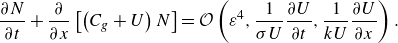 \begin{equation} \frac {\partial N}{\partial t} + \frac {\partial }{\partial x} \left [ \left (C_g + U\right ) N \right ] = {\mathcal{O}}\left (\varepsilon ^4, \frac {1}{\sigma U} \frac {\partial U}{\partial t}, \frac {1}{k U} \frac {\partial U}{\partial x}\right ). \end{equation}
Section 3.4 deals specifically with quantifying the ambient velocity variation in the context of long-wave orbital velocities.
There is an alternative derivation of the wave action conservation that was pointed out by Bretherton & Garrett (Reference Bretherton and Garrett1968). Starting from the wave energy conservation in non-uniform currents derived by Longuet-Higgins & Stewart (Reference Longuet-Higgins and Stewart1961)
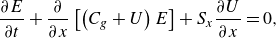 \begin{equation} \frac {\partial E}{\partial t} + \frac {\partial }{\partial x} \left [ \left (C_g + U\right ) E \right ] + S_{x} \frac {\partial U}{\partial x} = 0, \end{equation}
where $S_x$
is the wave radiation stress, and combining it with the dispersion relation (2.1) and conservation of crests (2.2), they show that (A26) is equivalent to the wave action conservation (2.3). This derivation is found in the Appendix of Bretherton & Garrett (Reference Bretherton and Garrett1968), and was later recognised by Whitham (Reference Whitham1974) as well.
$S_x$
is the wave radiation stress, and combining it with the dispersion relation (2.1) and conservation of crests (2.2), they show that (A26) is equivalent to the wave action conservation (2.3). This derivation is found in the Appendix of Bretherton & Garrett (Reference Bretherton and Garrett1968), and was later recognised by Whitham (Reference Whitham1974) as well.
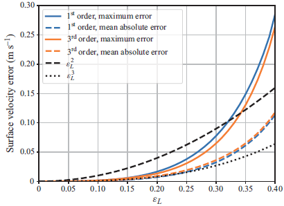
Figure 18. Surface velocity error as a function of wave steepness $\varepsilon _L$
, for the linear wave (blue) and the third-order Stokes wave (orange). Maximum and mean errors are indicated with solid and dashed lines, respectively. For reference,
$\varepsilon _L$
, for the linear wave (blue) and the third-order Stokes wave (orange). Maximum and mean errors are indicated with solid and dashed lines, respectively. For reference, $\varepsilon _L^2$
and
$\varepsilon _L^2$
and $\varepsilon _L^3$
curves are shown in black dashed and dotted lines, respectively.
$\varepsilon _L^3$
curves are shown in black dashed and dotted lines, respectively.
In summary, asymptotically consistent sets of dispersion and action conservation equations vary depending on the level of nonlinearity considered. In the case of linear waves, the dispersion relation (2.1), the averaged Lagrangian (A18), the adiabatic quantity (A21) and the wave action conservation (A23) are asymptotically consistent. For third-order Stokes waves, the dispersion relation (A7), the adiabatic quantity (A24), together with the group speed that includes a ${\mathcal{O}}(\varepsilon ^2)$
correction, are governed by the action conservation law (A23), but with the truncation error of
${\mathcal{O}}(\varepsilon ^2)$
correction, are governed by the action conservation law (A23), but with the truncation error of ${\mathcal{O}}(\varepsilon ^4)$
), and are asymptotically consistent. This is summarised in table 2.
${\mathcal{O}}(\varepsilon ^4)$
), and are asymptotically consistent. This is summarised in table 2.
Appendix B. Surface velocity errors
The long-wave induced velocities (2.7)–(2.9) are accurate to ${\mathcal{O}}(\varepsilon _L^3)$
when evaluated at the mean water level. However, in this paper we depart from the mean water level and evaluate the velocities at the surface of the long wave. This introduces additional errors at
${\mathcal{O}}(\varepsilon _L^3)$
when evaluated at the mean water level. However, in this paper we depart from the mean water level and evaluate the velocities at the surface of the long wave. This introduces additional errors at ${\mathcal{O}}(\varepsilon _L^2)$
. To quantify this error exactly, we compare the velocities evaluated at the surface for a linear (small-amplitude) wave and a third-order Stokes wave, with the surface velocity of a fully nonlinear wave (figure 17). The elevation and the surface velocity for the fully nonlinear wave is calculated numerically using the method by Clamond & Dutykh (Reference Clamond and Dutykh2018), which relies on Petviashvili’s iterations and in this case uses 2048 Fourier modes to represent the wave. Both the first-order and the third-order waves underestimate the surface velocity at the crest and in the trough, and overestimate it on the front and rear faces of the crest.
${\mathcal{O}}(\varepsilon _L^2)$
. To quantify this error exactly, we compare the velocities evaluated at the surface for a linear (small-amplitude) wave and a third-order Stokes wave, with the surface velocity of a fully nonlinear wave (figure 17). The elevation and the surface velocity for the fully nonlinear wave is calculated numerically using the method by Clamond & Dutykh (Reference Clamond and Dutykh2018), which relies on Petviashvili’s iterations and in this case uses 2048 Fourier modes to represent the wave. Both the first-order and the third-order waves underestimate the surface velocity at the crest and in the trough, and overestimate it on the front and rear faces of the crest.
Maximum values of surface velocity errors for both the linear and the third-order Stokes wave asymptote to $\varepsilon _L^3$
for small
$\varepsilon _L^3$
for small $\varepsilon _L$
(figure 18). However, they approach and exceed
$\varepsilon _L$
(figure 18). However, they approach and exceed $\varepsilon _L^2$
at
$\varepsilon _L^2$
at $\varepsilon _L \approx 0.3$
and beyond. Although the maximum error is
$\varepsilon _L \approx 0.3$
and beyond. Although the maximum error is ${\approx}10{-}20\, \%$
smaller for the third-order Stokes wave relative to the linear wave, its average error is slightly larger. The main takeaway from this figure is that evaluating the surface velocity of a linear wave carries an error no greater than
${\approx}10{-}20\, \%$
smaller for the third-order Stokes wave relative to the linear wave, its average error is slightly larger. The main takeaway from this figure is that evaluating the surface velocity of a linear wave carries an error no greater than $\varepsilon _L^2$
for
$\varepsilon _L^2$
for $\varepsilon _L \lt 0.32$
. Field measurements of near-surface orbital velocities by Laxague & Zappa (Reference Laxague and Zappa2020) qualitatively support this result, although they find larger departures from the linear theory in stronger winds, that is, steeper waves.
$\varepsilon _L \lt 0.32$
. Field measurements of near-surface orbital velocities by Laxague & Zappa (Reference Laxague and Zappa2020) qualitatively support this result, although they find larger departures from the linear theory in stronger winds, that is, steeper waves.


 Open access