Hostname: page-component-cd9895bd7-gxg78 Total loading time: 0 Render date: 2024-12-26T07:04:59.047Z Has data issue: false hasContentIssue false

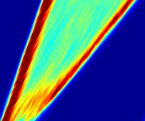
Scaling and mechanism of the propagation speed of the upstream turbulent front in pipe flow

Published online by Cambridge University Press:  21 December 2023

Haoyang Wu
Affiliation:
Center for Applied Mathematics, Tianjin University, Tianjin 300072, PR China
Baofang Song*
Affiliation:
State Key Laboratory of Turbulence and Complex Systems, College of Engineering, Peking University, Beijing 100871, PR China
*
Email address for correspondence: baofang.song@pku.edu.cn

Abstract

The scaling and mechanism of the propagation speed of turbulent fronts in pipe flow with the Reynolds number has been a long-standing problem in the past decades. Here, we derive an explicit scaling law for the upstream front speed, which approaches a power-law scaling at high Reynolds numbers, and we explain the underlying mechanism. Our data show that the average wall distance of low-speed streaks at the tip of the upstream front, where transition occurs, appears to be constant in local wall units in the wide bulk-Reynolds-number range investigated, between 5000 and 60 000. By further assuming that the axial propagation of velocity fluctuations at the front tip, resulting from streak instabilities, is dominated by the advection of the local mean flow, the front speed can be derived as an explicit function of the Reynolds number. The derived formula agrees well with the speed measured by front tracking. Our finding reveals a relationship between the structure and speed of a front, which enables a close approximation to be obtained of the front speed based on a single velocity field without having to track the front over time.

Type
JFM Rapids
Copyright
© The Author(s), 2023. Published by Cambridge University Press

1. Introduction

Front formation and propagation are important processes in nonlinear systems involving reaction, diffusion and advection, such as combustion, neural systems, epidemics and turbulent flows. In pipe flow, a localized turbulent region expands via the propagation of the upstream front (UF) and downstream front (DF) into the laminar region, where the flow is stable to infinitesimal perturbations (Meseguer & Trefethen Reference Meseguer and Trefethen2003; Chen, Wei & Zhang Reference Chen, Wei and Zhang2022b) – see figure 1 for an illustration. The front speeds determine the expansion rate of the turbulent region and consequently the wall friction. Therefore, front speed is an important characteristic of pipe-flow turbulence and, together with the front structure, has been the subject of many studies in the past six decades (Lindgren Reference Lindgren1957, Reference Lindgren1969; Wygnanski & Champagne Reference Wygnanski and Champagne1973; Darbyshire & Mullin Reference Darbyshire and Mullin1995; Shan et al. Reference Shan, Ma, Zhang and Nieuwstadt1999; Durst & Ünsal Reference Durst and Ünsal2006; van Doorne & Westerweel Reference van Doorne and Westerweel2008; Nishi et al. Reference Nishi, Ünsal, Durst and Biswas2008; Duguet, Willis & Kerswell Reference Duguet, Willis and Kerswell2010; Holzner et al. Reference Holzner, Song, Avila and Hof2013; Barkley et al. Reference Barkley, Song, Mukund, Lemoult, Avila and Hof2015; Barkley Reference Barkley2016; Song et al. Reference Song, Barkley, Hof and Avila2017; Rinaldi, Canton & Schlatter Reference Rinaldi, Canton and Schlatter2019; Chen, Xu & Song Reference Chen, Xu and Song2022a; Wang & Goldenfeld Reference Wang and Goldenfeld2022). Yet the mechanism that determines the front speed and the scaling of the speed with the Reynolds number (Re) remains largely unclear to date.

Figure 1. The expansion of turbulence at $Re=5000$. Contours of the magnitude of transverse velocity (averaged over the pipe cross-section) are plotted in the space (pipe axis) and time plane. The length unit in space is the pipe diameter $D$ and the time unit is $D/U_b$, with $U_b$ being the bulk speed of the flow. The main stream is from left to right, and time is vertically up. Red shows highly turbulent and blue shows laminar regions. The different slopes of the two red strips (fronts) indicate different front speeds, i.e. the turbulent region expands.

Most relevant studies have focused on the narrow regime of transition from localized puffs to expanding turbulent states, i.e. slugs, at relatively low Reynolds numbers of $O(10^3)$. Owing to difficulties of measuring front speed at high $Re$ (Chen et al. Reference Chen, Xu and Song2022a), especially for the DF, only Wygnanski & Champagne (Reference Wygnanski and Champagne1973) and Chen et al. (Reference Chen, Xu and Song2022a) considered higher $Re$ at $O(10^4)$. Reasonable agreement has been obtained among existing measurements for the UF speed, showing a monotonically decreasing trend as $Re$ increases – see Chen et al. (Reference Chen, Xu and Song2022a) and Avila, Barkley & Hof (Reference Avila, Barkley and Hof2023) for the latest literature reviews. However, Wygnanski & Champagne (Reference Wygnanski and Champagne1973) and Chen et al. (Reference Chen, Xu and Song2022a) reported opposite speed trends above $Re \simeq 10\,000$ for the DF. By direct numerical simulations (DNS) up to $Re=10^5$, Chen et al. (Reference Chen, Xu and Song2022a) reported fits $\tilde c_{UF}=0.024+(Re/1936)^{-0.528}$ for the UF and $\tilde {c}_{DF}=1.971-(Re/1925)^{-0.825}$ for the DF, and argued for monotonic trends of the two front speeds with $Re$ at high Reynolds numbers. Although fitting the measured speeds well, these are pure data fits with a prescribed form, but the underlying mechanism was left unexplained. In these fits and throughout this paper, the reference length and velocity are the pipe diameter $D$ and bulk speed $U_b$, respectively. The Reynolds number is defined as $Re=U_bD/\nu$, where $\nu$ is the kinematic viscosity. We will consider only the UF speed in this work.

Other than direct measurements of the front speed by tracking the front along the pipe axis, as in most studies, a few theoretical attempts have been made. For example, based on an energy flux analysis of the front region, without considering the dynamic transition process, Lindgren (Reference Lindgren1969) predicted an asymptotic speed of 0.69 as $Re\to \infty$. However, this prediction was questioned by both experimental (Wygnanski & Champagne Reference Wygnanski and Champagne1973) and numerical (Chen et al. Reference Chen, Xu and Song2022a) measurements, which showed much lower speeds than the asymptotic prediction of Lindgren (Reference Lindgren1969). Barkley et al. (Reference Barkley, Song, Mukund, Lemoult, Avila and Hof2015) and Barkley (Reference Barkley2016) used a theoretical model to investigate the front in the transitional regime, which captures the large-scale dynamics of the fronts successfully. The asymptotic analysis explains the front speed as a combination of the advection of the bulk turbulence and propagation with respect to the bulk turbulence (see figure 1). However, as a generic model for one-dimensional reaction–diffusion–advection systems, the model does not account for the three-dimensionality of the transition for pipe flow and does not give an explicit relationship between the front speed and $Re$. Besides, the $Re$ range considered was too narrow for a scaling with $Re$ to be established. Similar problems apply to the stochastic prey–predator model recently proposed by Wang & Goldenfeld (Reference Wang and Goldenfeld2022), which nevertheless can reproduce the basic phenomenology of the front of pipe flow in the transitional regime. In a word, there is still a big gap between experiments and theory.

In this paper, our goal is to derive a scaling law of the front speed by accounting for the transition at the front.

2. Results

Our starting point is the observation of our earlier work (Chen et al. Reference Chen, Xu and Song2022a) that transition to turbulence occurs continuously at the tip of a front (see the supplementary movie available at https://doi.org/10.1017/jfm.2023.1015), maintaining a characteristic propagation speed and a characteristic shape of the front against the distortion of the mean shear. For a UF, the front tip refers to its most upstream point. We propose that an evaluation of the radial position of the transition point at the front tip is crucial for determining the front speed. The questions are how to quantitatively determine this position and how to relate it to the front speed.

Before presenting our results, the set-up of the flow system and some notation should be explained. The flow is incompressible and constant-mass-flux-driven, and is solved in cylindrical coordinates, where $(r,\theta,z)$ denote radial, azimuthal and axial coordinates, respectively, and $u_r$, $u_\theta$ and $u_z$ denote the respective fluctuating velocity components in the three directions. The axial length of the pipe domain is $17.5D$ for $Re\leq 10\,000$ and $5D$ for higher $Re$. Readers are referred to Chen et al. (Reference Chen, Xu and Song2022a) for more details about the simulation of a front in a short periodic pipe.

We first show the flow structure at the tip of the UF. In figure 2(a), contours of the magnitude of transverse velocity fluctuation in the $z\unicode{x2013}r$ plane show that turbulence is concentrated near the wall and gradually spreads out towards the pipe centre while going downstream (see the supplementary movie for more details). Figure 2(b) shows the distribution of maximum $|u_z|$ and $|u_r|$ in the $r\unicode{x2013}\theta$ cross-section along the pipe axis. These curves also reflect that the flow is non-turbulent on the upstream side of the front tip and turbulent on the downstream side. Figure 2(c) shows that the flow features nearly straight and streamwise-elongated low-speed (blue) and high-speed (red) streaks on the upstream side, whereas the flow structure is less regular on the downstream side of the front tip. These plots (especially figure 2b) suggest that the tip of the UF should sit in the rough interval $z\in (3, 3.5)$. Figure 2(d) shows the contours of $u_z$ in the $r\unicode{x2013}\theta$ plane at $z=3.18$. Alternating high-speed (red spots) and low-speed streaks (blue spots) can be seen close to the wall, while the flow is laminar in the core region of the pipe.

Figure 2. Structure of a UF. (a) The tip part (the most upstream part) of a UF in a $z\unicode{x2013}r$ plane at $Re=40\,000$. Contours of the transverse velocity $(u_r^2+u_{\theta }^2)^{1/2}$ are plotted in the $z\unicode{x2013}r$ cross-section. The main flow is from left to right, the blue shows regions of low velocity fluctuation and the red shows regions of high velocity fluctuation. (b) The maximum of $|u_r|$ and $|u_z|$ in the $r\unicode{x2013}\theta$ cross-section plotted along the pipe axis. (c) Contours of $u_z$ in the $z\unicode{x2013}\theta$ plane at $r=0.47$, which show low-speed (blue) and high-speed (red) streaks. (d) Contours of $u_z$ in the $r\unicode{x2013}\theta$ cross-section at $z=3.18$. The circle, at $r=0.47$, shows the radial position of the $z\unicode{x2013}\theta$ plane in panel (c). This circle approximately shows the average position of low-speed streaks (blue spots) at this axial position.

Although a quantitative description of the transition mechanism at the UF tip is still lacking, the consensus seems to be that the transition is caused by instabilities of the low-speed streaks (Shimizu & Kida Reference Shimizu and Kida2009; Duguet et al. Reference Duguet, Willis and Kerswell2010; Hof et al. Reference Hof, De Lozar, Avila, Tu and Schneider2010), which may consist of more fundamental substructures according to Jiang et al. (Reference Jiang, Lee, Chen, Smith and Linden2020a,Reference Jiang, Lee, Smith, Chen and Lindenb). The instabilities here possibly coincide with those (either modal or non-modal) proposed for explaining either subcritical transition or the self-sustaining mechanism of shear-flow turbulence (Swearingen & Blackwelder Reference Swearingen and Blackwelder1987; Hamilton, Kim & Waleffe Reference Hamilton, Kim and Waleffe1995; Zikanov Reference Zikanov1996; Waleffe Reference Waleffe1997; Schoppa & Hussain Reference Schoppa and Hussain1998, Reference Schoppa and Hussain2002; Meseguer Reference Meseguer2003). In the following, we will establish a connection between the low-speed streaks and the front speed based on a few hypotheses, the first of which reads as follows:

  1. H1 The wall distance of the transition point at the front tip, in local wall units, is independent of the Reynolds number statistically.

This should be reasonable because the transition takes place near the wall, so that the wall distance of the transition point can be expected to scale with the wall length, which is the only length scale that can be derived from viscosity and wall shear. We will verify this hypothesis by measuring the wall distance of low-speed streaks as a proxy of that of the transition point.

At a turbulent front, the flow is axially developing, so that low-speed streaks are not parallel to the pipe wall but oblique, i.e. the wall distance varies along a streak. Figure 3(a,b) suggest that low-speed streaks are gradually lifted up away from the wall while going downstream. To show this variation more quantitatively, we take the following approach to determine the wall distance of low-speed streaks at a given axial location. In an $r\unicode{x2013}\theta$ cross-section, low-speed streaks can be detected by setting a proper threshold in $u_z$, and regions enclosed by contour lines of the specified threshold can be considered as (the cross-sections of) low-speed streaks – see the magenta contour lines in figure 3(a) with a threshold $-0.04$. (See Appendix A for a discussion on the threshold selection.) Then, the nominal wall distance of a streak can be defined as the wall distance of the minimum of $u_z$ within the streak. The average wall distance is calculated as the arithmetic mean of the wall distances of all the streaks detected in this pipe cross-section.

Figure 3. (ad) Axial variation of the low-speed streaks and (e) mean velocity profiles near the front tip. The flow field is the same as that shown in figure 2. (a)  Contours of $u_z$ at $z=3.0$. The contour level of $-0.04$ is plotted in magenta to highlight the low-speed streaks. (b) Contours at $z=3.3$. (c) The variation of the average wall distance of streaks (thick red) and $\max _{(r,\theta )}|u_r|$ (thin blue) along the pipe axis. (d) Also at $z=3.3$, and the contour level $0.025$ of the transverse velocity $(u_r^2+u_\theta ^2)^{1/2}$ is plotted in magenta to highlight the transverse velocity fluctuations. (e) The mean velocity profile at $z=3.3$, i.e. $U(r)=\langle u_x(r,\theta, 3.3)\rangle _{\theta }$, where $\langle {\cdot }\rangle _\theta$ means the average in the azimuthal direction. The parabolic profile is plotted as a broken line for comparison. The small window inset highlights the deviation between the two in the near-wall region.

Figure 3(c) shows more quantitatively that the wall distance of streaks increases on going downstream. Therefore, it is necessary to determine the axial position of the front tip for finally determining the wall distance of the streaks at the front tip. We use $\max _{(r,\theta )}|u_r|$, which is a function of $z$, as an indicator of the local flow state. This curve is smooth and slowly varying in the laminar region and wiggles around in the turbulent region – see figures 2(b) and 3(c). The axial location of the front tip can be estimated by the position separating the smooth and wiggling parts of the curve of $\max _{r,\theta }|u_r|$. We use an algorithm that detects abrupt changes of a curve for this purpose, which is built-in as the function findchangepts in MATLAB R2018a (see Appendix B for a brief description of the algorithm). The blue dot in figure 3(c) shows the separating point determined using this algorithm.

Figure 4(a) shows the average wall distance of streaks $y=0.5-r$ at the front tip in outer units. The larger $Re$, the smaller $y$, which can be expected. Figure 4(b) shows $y^+$, the wall distance in local wall length units $\sqrt {\nu /\tau _w}$, where $\tau _w$ is the local wall shear stress. Considering that the azimuthally averaged velocity profiles at these axial locations are nearly parabolic (see figure 3e), $\tau _w$ is simply approximated by the value of the parabolic profile. It appears that $y^+$ stays nearly constant in the wide $Re$ range considered, which supports our hypothesis H1 given the crucial role that low-speed streaks play in the transition.

Figure 4. The average wall distance of the low-speed streaks at the tip of the UF. (a) The distance in the outer length units. (b) The distance in the local wall units. At each $Re$, about 10–20 velocity snapshots are collected, giving approximately 100–200 low-speed streaks for the statistics. The standard deviation is plotted as the error bars. The dashed lines are (2.1) taking $A=16.7$, which is the average of $y^+$ over all $Re$ shown in panel (b).

Assuming this $Re$ independence, we derive the scaling law for the speed of the UF as follows. First, take the wall distance of the transition point at the front tip to be $y_F^+=A$, where $A$ is independent of $Re$. Then, in outer units, we have

(2.1)\begin{equation} y_F=y_F^+{/}Re_{\tau}=A/Re_{\tau}. \end{equation}

The local mean flow speed, i.e. the azimuthally averaged streamwise velocity at the radial position of the transition point, in outer units, can be approximated by the local laminar value

(2.2)\begin{equation} U(y_F)\approx 2-8(0.5-y_F)^2=8(A/Re_{\tau}-A^2/Re_{\tau}^2), \end{equation}

given that the mean velocity profile is nearly parabolic at the front tip. As the relationship between $Re$ and $Re_\tau$ is

(2.3)\begin{equation} Re_{\tau}=\sqrt{-\left.\frac{\mathrm{d}U(r)}{\mathrm{d}r}\right\vert_{r=0.5}Re} = 2\sqrt{2Re} \end{equation}

for a parabolic velocity profile, we have

(2.4)\begin{equation} U(y_F) \approx 2\sqrt{2}\,A\,Re^{{-}0.5} - A^2 Re^{{-}1}. \end{equation}

Now we come to our further hypotheses:

  1. H2 The wall distance of velocity perturbations at the front tip, resulting from streak instabilities, can be closely approximated by the wall distance of the streaks.

  2. H3 The front speed is determined by the axial propagation speed of these velocity perturbations, which approximately equals the local mean flow speed.

H2 should be reasonable, especially when perturbations appear at the flanks of the streaks. In fact, the data seem to support this hypothesis – see figure 3(d) where most of the strong perturbation region, enclosed by magenta contour lines, seems to be at the flanks of the low-speed streaks. H3 is based on our presumption that streak instabilities generate streamwise vortices, which further generate streaks while being advected downstream, seeding new transition and closing the self-sustaining cycle of the dynamics at the front tip. Therefore, the propagation speed of these vortices likely determines that of the front tip and consequently the front speed. The propagation of vortical structures, at least in fully developed wall turbulence above the viscous sublayer, was shown to be dominated by the advection of the local mean flow (Wu & Moin Reference Wu and Moin2008; Del Álamo & Jiménez Reference Del Álamo and Jiménez2009; Pei et al. Reference Pei, Chen, She and Hussain2012).

Following these hypotheses, we finally have an approximation of the front speed as

(2.5)\begin{equation} c_{UF}\approx U(y_F) \approx 2\sqrt{2}\,A\,Re^{{-}0.5} - A^2 Re^{ {-}1}, \end{equation}

and an asymptotic approximation at large $Re$,

(2.6)\begin{equation} c_{UF} \approx U(y_F)\approx 2\sqrt{2}\,A\,Re^{{-}0.5}, \end{equation}

where $A$ can be approximated by the wall distance of low-speed streaks at the front tip.

Figure 5 concludes the speed measurements and our derivation. The filled circles are the DNS data from Chen et al. (Reference Chen, Xu and Song2022a) (up to $Re=60\,000$) and the open symbols show the literature data in the $Re$ range investigated here. In order to show that the formula is predictive, DNS at $Re=80\,000$ is performed here, and the front speed is measured by front tracking and plotted as filled circles also. The black solid line shows our derivation (2.5) by setting $A=16.7$, which is the average of $y^+$ of streaks at all $Re$ values as shown in figure 4(b). The relative error of the prediction is on the level of a few per cent compared to the DNS measurement. The red dashed line shows the asymptotic speed (2.6) with the same $A$. Some former experimental measurements are also included in the figure. It should be noted that this formula can also be considered as a model for the front speed with only one parameter $A$, which has a physical meaning and, more precisely, should be interpreted as the wall distance of the transition point at the front tip. This formula can be used for other $Re$ after calibrating the parameter $A$ at one $Re$ with the measured front speed.

Figure 5. (a) Comparison of derived and measured front speeds. The circles show the speeds measured by front tracking using DNS (Chen et al. Reference Chen, Xu and Song2022a). The solid black line shows the approximation (2.5) with $A=16.7$, which is the average of the $y^+$ (black circles in figure 4b) over all $Re$ values. The dashed red line shows the approximation (2.6) with $A=16.7$ also. (b) The same plot in linear scale for the speed where some data sets from the literature falling in this $Re$ range are also included.

Now we revisit the fit $\tilde c_{UF}=0.024+(Re/1936)^{-0.528}$ given by Chen et al. (Reference Chen, Xu and Song2022a). This was obtained by assuming a form of $a+b\,Re^\beta$ without any explanation of the underlying physics. In other words, this form is not unique. Besides, the small constant 0.024 implies that the front speed would not approach zero as $Re$ approaches infinity, which was unexplained and seems counter-intuitive. It is probably just a result of measurement errors and the specific prescribed form of the fit. In contrast, our derivation (2.5) makes no assumption on the specific form of the formula. It follows naturally from the dynamics we observed at the front tip, with a few hypothetical but reasonable assumptions of the physics.

Our derivation (2.5) may suffer larger errors at lower $Re$. The low-speed streaks would be larger in transverse size at lower $Re$; therefore, the position of a streak estimated simply by the position of the minimum of $u_z$ in each streak becomes less representative. Besides, the streak position may not exactly coincide with the position of velocity fluctuations resulting from the streak instability. But these positions are close to each other at sufficiently high $Re$, so that our derivation will be more accurate.

As for the DF, the front speed is probably determined by the advection of the local mean flow at the front tip also. However, transition to turbulence occurs close to the pipe centre (Chen et al. Reference Chen, Xu and Song2022a) and the transition may not be triggered by streak instabilities as known for near-wall turbulence. Therefore, the location of the transition point may not scale with the wall length units, and cannot be explicitly related to $Re$ as shown here for the UF at the present. This problem has to be left for future studies.

3. Conclusions

In summary, the speed of the UF of pipe-flow turbulence was derived as an explicit function of $Re$ based on the dynamics at the front tip. To our knowledge, this is the first such work since the seminal measurements and theoretical analysis of Lindgren (Reference Lindgren1957, Reference Lindgren1969) about six decades ago. The agreement with speed measurements (see figure 5) suggests that the mechanism proposed here captures the core of the physics, i.e. the front speed is largely determined by the advection of velocity fluctuations by the local mean flow at the front tip where transition takes place. This mechanism may also apply to turbulent fronts in other shear flows where turbulence propagates into the subcritical laminar flow region. Although the local mean flow is different in higher dimensions such as planar shear flows (see e.g. Duguet & Schlatter Reference Duguet and Schlatter2013; Tao, Eckhardt & Xiong Reference Tao, Eckhardt and Xiong2018; Tuckerman, Chantry & Barkley Reference Tuckerman, Chantry and Barkley2020; Klotz, Pavlenko & Wesfreid Reference Klotz, Pavlenko and Wesfreid2021), our work will be helpful for elucidating the physics of front propagation in those flows.

Supplementary movie

A supplementary movie is available at https://doi.org/10.1017/jfm.2023.1015.

Funding

The authors acknowledge financial support from the National Natural Science Foundation of China under grant numbers 12272264 and 91852105. The work is also supported by The Fundamental Research Funds for the Central Universities, Peking University. Simulations were performed on Tianhe-2 at the National Supercomputer Centre in Guangzhou and on Tianhe-1(A) at the National Supercomputer Centre in Tianjin.

Declaration of interests

The authors report no conflict of interest.

Appendix A. Threshold for detecting streaks

The results presented in the main text take the threshold of $-0.04$. Here we explain the selection of this value. Figure 6 shows the contour levels of $-0.02$, $-0.04$ and $-0.06$ in the $r$$\theta$ cross-section at $z=3.18$, which is the same position as shown in figure 2(d) of the main text, plotted as magenta lines. It can be seen that $-0.02$ cannot very well separate adjacent streaks, whereas $-0.06$ may miss out many streaks. We checked multiple velocity snapshots and Reynolds numbers and found this to be often the case. The threshold $-0.04$ is a reasonable choice because, in most cases, it separates streaks well and is able to detect most of the low-speed streaks.

Figure 6. (ac) Thresholds for detecting low-speed streaks: $-0.02$, $-0.04$ and $-0.06$, respectively. Contours of streamwise velocity fluctuation in the $r$$\theta$ cross-section for $Re=40\,000$, as also shown in figure 2 of the main text. Contour levels of $-0.02$, $-0.04$ and $-0.06$ are plotted as magenta lines. (d) The average wall distance of low-speed streaks in wall units determined with thresholds of $-0.02$ (blue triangles), $-0.04$ (black circles) and $-0.06$ (red squares) in $u_z$ for detecting the streaks.

It can be expected that the value of this threshold will affect the average position of the streaks. A higher threshold may drop out weaker streaks and only retain stronger streaks. Stronger streaks are often more lifted up away from the wall (as can be seen in figure 6), and, therefore, a higher threshold will give a larger average wall distance of the streaks. Here we measured the average wall distance $y^+$ of the streaks determined using thresholds $-0.02$ and $-0.06$; see the blue triangles and red squares, respectively, in figure 6(d). It can be seen that $-0.02$ gives slightly lower and $-0.06$ gives slightly higher $y^+$ compared to the black circles (with a threshold of $-0.04$ for detecting streaks). But the important point is that $y^+$ also appears to be a constant in the $Re$ range considered using either threshold for detecting the streaks.

Appendix B. The algorithm for determining the axial location of the front tip

In the main text, we use the algorithm that is built-in as the function findchangepts in MATLAB to detect abrupt changes in a signal sequence $[x_1, x_2,\ldots, x_n]$. The key is to minimize the target function

(B1)\begin{align} J(k)=\sum_{i=1}^{k-1}\{x_i-{\rm mean}([x_1, x_2,\ldots,x_{k-1}])\}^2 +\sum_{i=k}^n\{x_i-{\rm mean}([x_k,x_{k+1},\ldots,x_n])\}^2 \end{align}

by modifying the index $k$. The resulting $k$ is regarded as the separation point of the slowly varying and abruptly varying parts of the sequence. The data sequence of $\max _{r,\theta }|u_r|$, containing both the laminar and turbulent parts on the upstream and downstream sides of the front tip, respectively, is fed in as the input. The output will be taken as the point separating the laminar part and the turbulent part of the curve, which we define as the axial location of the front tip. Readers are referred to the documentation of MATLAB (version R2018a) for more details about the algorithm.

References

Avila, M., Barkley, D. & Hof, B. 2023 Transition to turbulence in pipe flow. Annu. Rev. Fluid Mech. 55, 575602.CrossRefGoogle Scholar
Barkley, D. 2016 Theoretical perspective on the route to turbulence in a pipe. J. Fluid Mech. 803, P1.CrossRefGoogle Scholar
Barkley, D., Song, B., Mukund, V., Lemoult, G., Avila, M. & Hof, B. 2015 The rise of fully turbulent flow. Nature 526, 550553.CrossRefGoogle ScholarPubMed
Chen, K., Xu, D. & Song, B. 2022 a Propagation speed of turbulent fronts in pipe flow at high Reynolds numbers. J. Fluid Mech. 935, A11.CrossRefGoogle Scholar
Chen, Q., Wei, D. & Zhang, Z. 2022 b Linear stability of pipe Poiseuille flow at high Reynolds number regime. Commun. Pure Appl. Maths 76, 18681964.CrossRefGoogle Scholar
Darbyshire, A.G. & Mullin, T. 1995 Transition to turbulence in constant-mass-flux pipe flow. J. Fluid Mech. 289, 83114.CrossRefGoogle Scholar
Del Álamo, J.C. & Jiménez, J. 2009 Estimation of turbulent convection velocities and corrections to Taylor's approximation. J. Fluid Mech. 640, 526.CrossRefGoogle Scholar
van Doorne, C.W.H. & Westerweel, J. 2008 The flow structure of a puff. Phil. Trans. R. Soc. Lond. A 367, 489507.Google Scholar
Duguet, Y. & Schlatter, P. 2013 Oblique laminar-turbulent interfaces in plane shear flows. Phys. Rev. Lett. 110, 034502.CrossRefGoogle ScholarPubMed
Duguet, Y., Willis, A.P. & Kerswell, R.R. 2010 Slug genesis in cylindrical pipe flow. J. Fluid Mech. 663, 180208.CrossRefGoogle Scholar
Durst, F. & Ünsal, B. 2006 Forced laminar to turbulent transition in pipe flows. J. Fluid Mech. 560, 449464.CrossRefGoogle Scholar
Hamilton, J.M., Kim, J. & Waleffe, F. 1995 Regeneration mechanisms of near-wall turbulent structures. J. Fluid Mech. 287, 317348.CrossRefGoogle Scholar
Hof, B., De Lozar, A., Avila, M., Tu, X. & Schneider, T.M. 2010 Eliminating turbulence in spatially intermittent flows. Science 327, 14911494.CrossRefGoogle ScholarPubMed
Holzner, M., Song, B., Avila, M. & Hof, B. 2013 Lagrangian approach to laminar-turbulent interfaces. J. Fluid Mech. 723, 140162.CrossRefGoogle Scholar
Jiang, X.Y., Lee, C.B., Chen, X., Smith, C.R. & Linden, P.F. 2020 a Structure evolution at early stage of boundary-layer transition: simulation and experiment. J. Fluid Mech. 890, A11.CrossRefGoogle Scholar
Jiang, X.Y., Lee, C.B., Smith, C.R., Chen, J.W. & Linden, P.F. 2020 b Experimental study on low-speed streaks in a turbulent boundary layer at low Reynolds number. J. Fluid Mech. 903, A6.CrossRefGoogle Scholar
Klotz, L., Pavlenko, A.M. & Wesfreid, J.E. 2021 Experimental measurements in plane Couette–Poiseuille flow: dynamics of the large-and small-scale flow. J. Fluid Mech. 912, A24.CrossRefGoogle Scholar
Lindgren, E.R. 1957 The transition process and other phenomena in viscous flow. Ark. Fys. 12, 1169.Google Scholar
Lindgren, E.R. 1969 Propagation velocity of turbulent slugs and streaks in transition pipe flow. Phys. Fluids 12, 418425.CrossRefGoogle Scholar
Meseguer, A. 2003 Streak breakdown instability in pipe Poiseuille flow. Phys. Fluids 15, 12031213.CrossRefGoogle Scholar
Meseguer, A. & Trefethen, L.N. 2003 Linearized pipe flow to Reynolds number $10^7$. J. Comput. Phys. 186, 178197.CrossRefGoogle Scholar
Nishi, M., Ünsal, B., Durst, F. & Biswas, G. 2008 Laminar-to-turbulent transition of pipe flows through puffs and slugs. J. Fluid Mech. 614, 425446.CrossRefGoogle Scholar
Pei, J., Chen, J., She, Z.-S. & Hussain, F. 2012 Model for propagation speed in turbulent channel flows. Phys. Rev. E 86, 046307.CrossRefGoogle ScholarPubMed
Rinaldi, E., Canton, J. & Schlatter, P. 2019 The vanishing of strong turbulent fronts in bent pipes. J. Fluid Mech. 866, 487502.CrossRefGoogle Scholar
Schoppa, W. & Hussain, F. 1998 Formation of near-wall streamwise vortices by streak instability. AIAA Paper 98, 3000.Google Scholar
Schoppa, W. & Hussain, F. 2002 Coherent structure generation in near-wall turbulence. J. Fluid Mech. 453, 57108.CrossRefGoogle Scholar
Shan, X., Ma, B., Zhang, Z. & Nieuwstadt, F.T.M. 1999 Direct numerical simulation of a puff and a slug in transitional cylindrical pipe flow. J. Fluid Mech. 387, 3960.CrossRefGoogle Scholar
Shimizu, M. & Kida, S. 2009 A driving mechanism of a turbulent puff in pipe flow. Fluid Dyn. Res. 41, 045501.CrossRefGoogle Scholar
Song, B., Barkley, D., Hof, B. & Avila, M. 2017 Speed and structure of turbulent fronts in pipe flow. J. Fluid Mech. 813, 10451059.CrossRefGoogle Scholar
Swearingen, J.D. & Blackwelder, R.F. 1987 The growth and breakdown of streamwise vortices in the presence of a wall. J. Fluid Mech. 182, 255290.CrossRefGoogle Scholar
Tao, J.J., Eckhardt, B. & Xiong, X.M. 2018 Extended localized structures and the onset of turbulence in channel flow. Phys. Rev. Fluids 3, 011902(R).CrossRefGoogle Scholar
Tuckerman, L.S., Chantry, M. & Barkley, D. 2020 Patterns in wall bounded shear flows. Annu. Rev. Fluid Mech. 52, 343367.CrossRefGoogle Scholar
Waleffe, F. 1997 On a self-sustaining process in shear flows. Phys. Fluids 9, 883900.CrossRefGoogle Scholar
Wang, M. & Goldenfeld, N. 2022 Stochastic model for quasi-one-dimensional transitional turbulence with streamwise shear interactions. Phys. Rev. Lett. 129, 034501.CrossRefGoogle ScholarPubMed
Wu, X. & Moin, P. 2008 A direct numerical simulation study on the mean velocity characteristics in turbulent pipe flow. J. Fluid Mech. 608, 81112.CrossRefGoogle Scholar
Wygnanski, I.J. & Champagne, F.H. 1973 On transition in a pipe. Part 1. The origin of puffs and slugs and the flow in a turbulent slug. J. Fluid Mech. 59, 281335.CrossRefGoogle Scholar
Zikanov, O.Y. 1996 On the instability of pipe Poiseuille flow. Phys. Fluids 8, 29232932.CrossRefGoogle Scholar
Figure 0

Figure 1. The expansion of turbulence at $Re=5000$. Contours of the magnitude of transverse velocity (averaged over the pipe cross-section) are plotted in the space (pipe axis) and time plane. The length unit in space is the pipe diameter $D$ and the time unit is $D/U_b$, with $U_b$ being the bulk speed of the flow. The main stream is from left to right, and time is vertically up. Red shows highly turbulent and blue shows laminar regions. The different slopes of the two red strips (fronts) indicate different front speeds, i.e. the turbulent region expands.

Figure 1

Figure 2. Structure of a UF. (a) The tip part (the most upstream part) of a UF in a $z\unicode{x2013}r$ plane at $Re=40\,000$. Contours of the transverse velocity $(u_r^2+u_{\theta }^2)^{1/2}$ are plotted in the $z\unicode{x2013}r$ cross-section. The main flow is from left to right, the blue shows regions of low velocity fluctuation and the red shows regions of high velocity fluctuation. (b) The maximum of $|u_r|$ and $|u_z|$ in the $r\unicode{x2013}\theta$ cross-section plotted along the pipe axis. (c) Contours of $u_z$ in the $z\unicode{x2013}\theta$ plane at $r=0.47$, which show low-speed (blue) and high-speed (red) streaks. (d) Contours of $u_z$ in the $r\unicode{x2013}\theta$ cross-section at $z=3.18$. The circle, at $r=0.47$, shows the radial position of the $z\unicode{x2013}\theta$ plane in panel (c). This circle approximately shows the average position of low-speed streaks (blue spots) at this axial position.

Figure 2

Figure 3. (ad) Axial variation of the low-speed streaks and (e) mean velocity profiles near the front tip. The flow field is the same as that shown in figure 2. (a)  Contours of $u_z$ at $z=3.0$. The contour level of $-0.04$ is plotted in magenta to highlight the low-speed streaks. (b) Contours at $z=3.3$. (c) The variation of the average wall distance of streaks (thick red) and $\max _{(r,\theta )}|u_r|$ (thin blue) along the pipe axis. (d) Also at $z=3.3$, and the contour level $0.025$ of the transverse velocity $(u_r^2+u_\theta ^2)^{1/2}$ is plotted in magenta to highlight the transverse velocity fluctuations. (e) The mean velocity profile at $z=3.3$, i.e. $U(r)=\langle u_x(r,\theta, 3.3)\rangle _{\theta }$, where $\langle {\cdot }\rangle _\theta$ means the average in the azimuthal direction. The parabolic profile is plotted as a broken line for comparison. The small window inset highlights the deviation between the two in the near-wall region.

Figure 3

Figure 4. The average wall distance of the low-speed streaks at the tip of the UF. (a) The distance in the outer length units. (b) The distance in the local wall units. At each $Re$, about 10–20 velocity snapshots are collected, giving approximately 100–200 low-speed streaks for the statistics. The standard deviation is plotted as the error bars. The dashed lines are (2.1) taking $A=16.7$, which is the average of $y^+$ over all $Re$ shown in panel (b).

Figure 4

Figure 5. (a) Comparison of derived and measured front speeds. The circles show the speeds measured by front tracking using DNS (Chen et al.2022a). The solid black line shows the approximation (2.5) with $A=16.7$, which is the average of the $y^+$ (black circles in figure 4b) over all $Re$ values. The dashed red line shows the approximation (2.6) with $A=16.7$ also. (b) The same plot in linear scale for the speed where some data sets from the literature falling in this $Re$ range are also included.

Figure 5

Figure 6. (ac) Thresholds for detecting low-speed streaks: $-0.02$, $-0.04$ and $-0.06$, respectively. Contours of streamwise velocity fluctuation in the $r$$\theta$ cross-section for $Re=40\,000$, as also shown in figure 2 of the main text. Contour levels of $-0.02$, $-0.04$ and $-0.06$ are plotted as magenta lines. (d) The average wall distance of low-speed streaks in wall units determined with thresholds of $-0.02$ (blue triangles), $-0.04$ (black circles) and $-0.06$ (red squares) in $u_z$ for detecting the streaks.

Supplementary material: File

Wu and Song supplementary movie

Contours of the transverse velocity fluctuations on a crosssection along the pipe axis in a frame of reference co-moving with the upstream front of a pipe flow at Re = 25000. It is upstream on the left and downstreamm on the right. The movie shows that transition to turbulence continuously occurs at the tip of the front (the most upstream part of the front) and turbulence spreads toward the pipe center while going downstream.
Download Wu and Song supplementary movie(File)
File 4.2 MB