Shape optimisation for a stochastic two-dimensional cylinder wake using ensemble variation

Abstract

In the present study, the shape of a two-dimensional cylinder is optimised to minimise the mean drag in laminar unsteady flow under a noisy environment. A small inline stochastic oscillation in the free-stream velocity, which follows the Ornstein–Uhlenbeck process, is considered for the noise. The small noise is found to yield a large random fluctuation in instantaneous drag of the cylinder due to the effect of added mass. Subject to the strong random fluctuation of drag, the shape optimisation is performed using an ensemble-variation-based method (EnVar), as the conventional adjoint-based optimisation is not applicable to such a flow environment with unknown free-stream noise. The optimised cylinder geometry is found to be a nearly-symmetric slender oval at a low Reynolds number. As the Reynolds number is increased, two optimal shapes emerge: one is identical to the oval obtained at the low Reynolds number, and the other is an asymmetric oval, the rear side of which is more slender than the front side, reminiscent of an aerofoil. Despite the large random fluctuation in the instantaneous drag, the optimal cylinder shapes obtained for different levels of the upstream noise are found to be almost identical. It is shown that the robust nature of the optimal cylinder shape originates from the limited influence of the small upstream noise on the mean flow properties of the cylinder wake. Finally, the optimised cylinder primarily reduces the pressure component of the drag, associated mainly with vortex shedding in the wake, and this is achieved by marginally increasing the viscous drag through the shape change.

1. Introduction

The wake behind a bluff body is an important canonical flow encountered in many engineering applications. Vortex shedding in the near-wake region is the main cause of drag, vibration and noise generation. Significant efforts have been made to control and mitigate vortex shedding. Depending on the presence of energy input given to the wake, the efforts may be classified into two categories (Choi, Jeon & Kim 2008): active and passive controls. Active control typically requires an actuation mechanism of mass and/or momentum to the flow, with consumption of the related energy. The examples include basebleed (Bearman 1967; Wood 1967), rotary and transverse oscillations of a cylinder (Tokumaru & Dimotakis 1991; Baek & Sung 1998; Blackburn & Henderson 1999; Choi, Choi & Kang 2002), and steady blowing/suction at the wall (Min & Choi 1999; Arcas & Redekopp 2004; Mao, Blackburn & Sherwin 2015). On the contrary, passive control does not require such an actuation mechanism, thereby not requiring extra energy input. The examples include a splitter plate (Roshko 1955; Bearman 1965; Kwon & Choi 1996), a secondary cylinder placed in the near-wake region (Strykowski & Sreenivasan 1990), spanwise geometrical undulation of the cylinder (Tombazis & Bearman 1997; Bearman & Owen 1998; Darekar & Sherwin 2001), and small spanwise localised tabs (Park et al. 2006). Given that the passive control does not need any sophisticated apparatus implementing any actuation mechanisms, it is more practical and robust than the active counterpart, providing a more pragmatic solution to many engineering applications.

An ultimate form of passive flow control is optimal shape design, which deforms the geometry of the cylinder to maximise or minimise the given objective functional. A well-established approach to optimal shape design is based on the calculus of variation utilising adjoint variables (see e.g. Pironneau 1974; Mohammadi & Pironneau 2009). This approach is basically identical to that used in optimal control (e.g. Abergel & Temam 1990; Bewley, Moin & Temam 2001), and the adjoint variables appear as the Lagrange multiplier characterising the gradient (or sensitivity) of the given objective functional. The approach and its variants have been employed previously for the design of a two-dimensional diffuser using a Reynolds-averaged Navier–Stokes model (Lim & Choi 2004), steady blowing/suction in a circular cylinder wake (Min & Choi 1999; Mao et al. 2015), structural sensitivities of the cylinder wake to small perturbations such as a secondary cylinder (Giannetti & Luchini 2007; Marquet, Sipp & Jacquin 2008), evaluation of the shape sensitivity of linear global mode in a circular cylinder wake (Brewster & Juniper 2020), and shape optimisation of a baffle to suppress turbulence in transitional pipe flow (Marensi, Willis & Kerswell 2020). Despite the successful examples, it is generally challenging to apply the adjoint-based optimisation for fluid systems subject to external noise and turbulent flows. In the former case, the objective functional may well be sensitive to external noise or disturbances in a certain flow configuration. Therefore, it may be possible that the optimisation performed under noise-free conditions does not necessarily provide a robust solution, implying that the given optimal solution may not be reliable in practice. In the latter case, where the given flow is turbulent, the adjoint-based optimisation approach is known to be technically problematic. The well-known ‘butterfly effect’ in such a chaotic system (i.e. the sensitivity dependence on initial conditions) means that the linearised Navier–Stokes equations about a turbulent state lead the solution to blow up in time due to unstable leading Lyapunov exponents. Given that the equations for adjoint variables share the same stability properties with the linearised Navier–Stokes equations, this implies that the adjoint equations are ill-posed for the evaluation of the gradient of the given objective functional because their solution would also blow up in time. To overcome this difficulty, several algorithms have been proposed recently (e.g. Wang, Hu & Blonigan 2014; Lasagna 2018; Lasagna, Sharma & Meyers 2019; Ni et al. 2019). However, the proposed algorithms are computationally highly demanding. Importantly, it has been shown recently that the leading Lyapunov exponent grows faster than the inverse of the Kolmogorov time scale with Reynolds number (Mohan, Fitzsimmons & Moser 2017), making their applications practically not attractive at high Reynolds numbers.

The ensemble variation (EnVar) is an alternative data-driven approach bypassing this technical difficulty in the optimisation of chaotic dynamical systems. It is a stochastic optimisation method, which refers to an approach that generates and uses random numbers for the formulation of the optimisation problem. For an introductory overview on stochastic optimisation methods, the reader may refer to Spall (2003). While the utilisation of random numbers can exist in any step of the given optimisation method, in the case of EnVar, a Monte Carlo method is forged inherently to approximate efficiently the gradient of the given objective functional. This approach originates from data assimilation adopted widely in meteorology (e.g. Lewis, Lakshmivarahan & Dhall 2006; Evensen 2009), and it has been popular increasingly in fluid mechanics (Colburn, Cessna & Bewley 2011; Suzuki 2012; Kato et al. 2015; Mons et al. 2016; Jahanbakhshi & Zaki 2019; Mons, Du & Zaki 2021). The ensemble variation is based on a data set (i.e. ensemble) from a large number of realisations (i.e. simulations or experiments), which are then exploited to approximate the given objective functional in the subspace spanned by the ensemble. Therefore, the given optimisation problem can be tackled in the subspace spanned by the ensemble, without solving the adjoint equations to evaluate the gradient of the objective functional. This feature is particularly useful to optimise the flow in the presence of noise and turbulent flow. Indeed, several recent studies have employed this approach successfully in several fluid mechanics problems, showing some promising performance for wider applications: for example, design of an ensemble Kármán filter (Colburn et al. 2011; Suzuki 2012), ensemble-variation-based optimal control (Yang et al. 2015), data-driven flow reconstruction (Kato et al. 2015; Mons et al. 2016), nonlinear optimal perturbation for boundary-layer transition (Jahanbakhshi & Zaki 2019), and subgrid-scale stress modelling for large-eddy simulations (Mons et al. 2021).

The objective of the present study is to apply the ensemble variation to shape optimisation problems. In particular, we will consider a two-dimensional laminar cylinder wake subject to free-stream noise. It is evident that this problem cannot be tackled with the classical adjoint-based optimisation technique, as the free-stream noise has to be assumed to be unknown in practical applications. Importantly, almost every flow control strategy for bluff-body wakes mentioned earlier was designed and tested in a highly controlled flow environment, i.e. well-resolved numerical simulations or well-controlled laboratory experiments (see Choi et al. 2008). Therefore, the robustness of the flow control strategies to external noise largely remains unexplored, even though it would be very common that many flow control devices in practical applications would experience such external noise. Indeed, accounting for robustness of a given control strategy (i.e. disturbance rejection) has been an important subject in modern control theories for linear dynamical systems (e.g. $\mathcal {H}_\infty$-looping shape, LQG control, etc.; see Zhou, Doyle & Glover 1996). In this respect, it is now timely to consider the effect of external noise on flow control and optimisation, and the ensemble-variation-based optimisation considered here would provide a solution for this type of problem.

This paper is organised as follows. In § 2, an ensemble-variation-based optimisation used in this study is introduced briefly with the formulation of the shape optimisation problem of the cylinder and the corresponding numerical method. The optimisation result is reported in § 3 with discussions on the robustness and the physical processes involved. The paper concludes in § 4.

2. Problem formulation

2.1. Ensemble-based variational optimisation

The ensemble-based variational method is a data-driven approach that approximates the gradient of an objective functional with respect to the desired design parameters using the outcomes of numerical simulations or experiments. Let us consider a dynamical system with the state vector $\boldsymbol {q}$ (i.e. velocity and pressure from the Navier–Stokes equations):

(2.1)\begin{equation} \boldsymbol{q} = \mathcal{N}(\boldsymbol{c},\boldsymbol{s}), \end{equation}

where $\boldsymbol {c}\in \mathbb {R}^{N_{{D}}}$ is the vector-valued optimisation control parameter with the number of degrees of freedom $N_{{D}}$, and $\boldsymbol {s}$ represents other system parameters, including the initial and boundary conditions. The objective functional $J$ is often defined in terms of the state vector $\boldsymbol {q}$, such that

(2.2)\begin{equation} J\left(\boldsymbol{c}\right) = \mathcal{F}(\boldsymbol{q}(\boldsymbol{c},\boldsymbol{s})). \end{equation}

From the combination of (2.1) and (2.2), the following general constrained optimisation problem may be formulated:

(2.3)\begin{equation} \left. \begin{aligned} & \underset{\boldsymbol{c}}{\min} \ {J}(\boldsymbol{c}) \quad \text{subject to}\\ & \boldsymbol{q} = \mathcal{N}(\boldsymbol{c}, \boldsymbol{s}), \\ & \boldsymbol{g}(\boldsymbol{c}) = \boldsymbol{m}, \\ & h_1(\boldsymbol{c}) \leq d_1, \quad \ldots,\quad h_{N_{ie}}(\boldsymbol{c}) \leq d_{N_{ieq}}, \end{aligned} \right\} \end{equation}

where the third line represents a vector form of equality constraints with $\boldsymbol {g}, \boldsymbol {m} \in \mathbb {R}^{N_{eq}}$, and the fourth line indicates inequality constraints with their number $N_{ieq}$.

Now we describe the solution procedure of (2.3). We first consider ${N_{en}}$, the number of simulation or experimental data points obtained by randomly varying the control parameter $\boldsymbol {c}$ around its mean $\boldsymbol {c}^{(e)}$ (or the initial guess of the solution to (2.3)). Without loss of generality, the control vector around $\boldsymbol {c}^{(e)}$ is expressed as a weighted sum:

(2.4a)\begin{equation} \boldsymbol{c} = \boldsymbol{c}^{(e)} + \boldsymbol{E}'\boldsymbol{w}, \end{equation}

where $\boldsymbol {w}\in \mathbb {R}^{N_{en}}$ is the weight vector, and $\boldsymbol {E}'\in \mathbb {R}^{N_{D}\times N_{en}}$ is the deviation matrix, which contains the deviations of the ensemble members $\boldsymbol {c}^{(r)}$ from their mean $\boldsymbol {c}^{(e)}$, i.e.

(2.4b) \begin{equation} \boldsymbol{E}' = \left[ \begin{array}{@{}ccccc@{}} \boldsymbol{c}^{(1)}-\boldsymbol{c}^{(e)} & \ldots & \boldsymbol{c}^{(r)}-\boldsymbol{c}^{(e)} & \ldots & \boldsymbol{c}^{(N_{en})}-\boldsymbol{c}^{(e)}\end{array} \right]. \end{equation}

Equation (2.4a) now approximates the control vector $\boldsymbol {c}$ around $\boldsymbol {c}^{(e)}$ in terms of the weight vector $\boldsymbol {w}$ – this is to convert the optimisation problem defined in terms of $\boldsymbol {c}$ into one in terms of $\boldsymbol {w}$ using the ensemble member (or data) $\boldsymbol {c}^{(r)}$. For $\lVert \boldsymbol {E}'\boldsymbol {w}\rVert _2 \ll 1$, where $\lVert \cdot \rVert _2$ is the standard ${l}_2$-norm, the state vector in (2.1) is approximated as

(2.5)\begin{equation} \boldsymbol{q} \simeq \boldsymbol{q}^{(e)} + \frac{\partial \mathcal{N}}{\partial \boldsymbol{c}}\bigg|_{\boldsymbol{c}^{(e)}}\boldsymbol{E}'\boldsymbol{w}, \end{equation}

where $\boldsymbol {q}^{(e)}=\mathcal {N}(\boldsymbol {c}^{(e)},\boldsymbol {s})$. Similarly, substitution of (2.5) into (2.2) yields

(2.6a)\begin{equation} J(\boldsymbol{c}(\boldsymbol{w})) \simeq \mathcal{F}(\boldsymbol{q}^{(e)}) +\boldsymbol{H}\boldsymbol{w}, \end{equation}

where

(2.6b)\begin{equation} \boldsymbol{H} = \left.\frac{\partial\mathcal{F}}{\partial\boldsymbol{q}}\right|_{\boldsymbol{q}^{(e)}} \left.\frac{\partial \mathcal{N}}{\partial \boldsymbol{c}}\right|_{\boldsymbol{c}^{(e)}}\boldsymbol{E}'. \end{equation}

Here, it is useful to mention that the matrix $\boldsymbol {H}$ can be approximated directly from the given objective functional instead of applying the chain rule in (2.6b):

(2.6c) \begin{align} \boldsymbol{H} = \left[ \begin{array}{@{}ccccc@{}} \mathcal{F}\left(\boldsymbol{q}^{(1)}\right) - \mathcal{F}\left(\boldsymbol{q}^{(e)}\right) & \ldots & \mathcal{F}\left(\boldsymbol{q}^{(r)}\right) - \mathcal{F}\left(\boldsymbol{q}^{(e)}\right) & \ldots & \mathcal{F}\left(\boldsymbol{q}^{(N_{en})}\right) - \mathcal{F}\left(\boldsymbol{q}^{(e)}\right) \end{array} \right], \end{align}

where $\boldsymbol {q}^{(r)}=\mathcal {N}(\boldsymbol {c}^{(r)},\boldsymbol {s})$.

Now, from (2.6a), the objective functional is given explicitly in terms of the weight vector $\boldsymbol {w}$. This can then be used to approximate the gradient (or the leading-order variation) of the objective functional $J$ with respect to the control vector $\boldsymbol {c}$, such that

(2.7)\begin{equation} \frac{\partial J}{\partial \boldsymbol{c}}\bigg|_{\boldsymbol{c}^{(e)}} {\boldsymbol{E}'}\simeq \boldsymbol{H}, \end{equation}

subject to the given equality and inequality constraints.

Some remarks on (2.7) are also useful here. First, like a typical gradient-based optimisation algorithm, the gradient of the objective functional approximated in (2.7) can now be used to iteratively find the solution to the optimisation problem (2.3). Typically, at each iteration, the control vector is updated combining the gradient in (2.7) with a suitable step size of the control vector determined using a line search algorithm. However, this procedure may be replaced conveniently by searching for the local optimum of the optimisation problem (2.3) within the small neighbourhood of $\boldsymbol {c}^{(e)}$ (with $\lVert \boldsymbol {w}\rVert _2 \ll 1$) at each iteration step. Indeed, for $\lVert \boldsymbol {w}\rVert _2 \ll 1$ and $\lVert \boldsymbol {H}\boldsymbol {w}\rVert _2 \ll 1$ expected from $\lVert \boldsymbol {E}'\boldsymbol {w}\rVert _2 \ll 1$, (2.3) can be converted into a convex optimisation problem using (2.7). For example, the nonlinear objective functional may be approximated as a linear function of $\boldsymbol {w}$, i.e.

(2.8)\begin{equation} J(\boldsymbol{c}(\boldsymbol{w}))\simeq J(\boldsymbol{c}^{(e)})+\frac{\partial J}{\partial \boldsymbol{c}}\bigg|_{\boldsymbol{c}^{(e)}}{\boldsymbol{E}'} \boldsymbol{w}\simeq J(\boldsymbol{w}=0) + \frac{\partial \mathcal{F}}{\partial \mathcal{G}}\bigg|_{\boldsymbol{o}^{(e)}} \boldsymbol{H} \boldsymbol{w}. \end{equation}

Similarly, the equality and inequality constraints in (2.3) may also be converted into linear or quadratic constraints with respect to the weight vector $\boldsymbol {w}$. Then this ‘local’ optimisation problem defined for $\lVert \boldsymbol {w}\rVert _2 \ll 1$ can be solved to obtain the optimal weight vector $\boldsymbol {w}$ by means of a wide variety of methods available (e.g. the interior point algorithm; see Nocedal & Wright 2006). Once the optimal weight vector is found by solving the local optimisation problem, it is updated as a new mean control vector for the next iteration as in the other gradient-based optimisation algorithms. This process can be repeated until the full solution of (2.3) is finally found. This solution procedure was proposed by Jahanbakhshi & Zaki (2019) and is employed in the present study.

Second, in the EnVar algorithm of this study, the optimal control vector is searched within the subspace spanned by the column vectors in $\boldsymbol {E}'$. Therefore, the control vectors $\boldsymbol {c}^{(r)}$ need to be generated by satisfying the constraints in (2.3). Furthermore, given $N_{D}$ degrees of freedom of the control vector, the minimum number of simulation or experimental data points $N_{en}$ for a well-defined local optimisation problem (2.3) is required theoretically to be

(2.9)\begin{equation} N_{en} = N_{D} - N_{eq}. \end{equation}

Such a situation occurs when all the column vectors in $\boldsymbol {E}'$ are linearly independent and the sampled data satisfy the given inequality constraints. However, in practice, $N_{en}$ of simulation or experimental data is not always required, because the gradient of the objective functional $J$ at each iteration step may well be approximated with degrees of freedom smaller than $N_{en}$. Indeed, the important low-dimensional subspace of the control vector providing a good approximation for the gradient of the given objective functional may well be identified by applying the singular value decomposition to $\boldsymbol {E}'$ with $N_{en} < N_{D} - N_{eq}$, as suggested by Jahanbakhshi & Zaki (2019). This procedure was adopted in the present study, although the number of samples for each ensemble is set to satisfy (2.9) (see § 3.1). The procedure generating the control vectors $\boldsymbol {c}^{(r)}$ also follows Jahanbakhshi & Zaki (2019), and the reader may refer to that study for further details.

2.2. Optimal shape design for stochastic cylinder wake

We consider a two-dimensional laminar flow over a cylinder with an arbitrary shape to find the optimal geometry that minimises the mean drag. To introduce noise to the flow, a time-dependent free-stream velocity $U(t)$ is considered with its time average $\bar {U}$. The equations of motion are made dimensionless using the mean free-stream velocity $\bar {U}$ and the length scale defined as the diameter of an equivalent circular cylinder of the same cross-sectional area, $L = 2\sqrt{A/{\rm \pi}}$, with $A$ being the area of the cylinder. The Reynolds number is then defined as $Re=\rho \bar {U} L/ \mu$, where $\rho$ is the fluid density and $\mu$ is the dynamic viscosity. Figure 1 shows a schematic sketch of the given flow configuration with the boundary conditions

(2.10a)$$\begin{gather} u = v = 0,\quad \text{on} \ \partial\varOmega_{{wall}}, \end{gather}$$

(2.10b)$$\begin{gather}u = \frac{U(t)}{\bar{U}}, v = 0 ,\quad\ \text{on}\ \partial\varOmega_{{inlet}}, \end{gather}$$

(2.10c)$$\begin{gather}\frac{\partial u}{\partial y} = v = 0,\quad \text{on}\ \partial\varOmega_{{top}} \cup \partial\varOmega_{{bottom}}, \end{gather}$$

(2.10d)$$\begin{gather}\frac{\partial u}{\partial x} = \frac{\partial v}{\partial x} = 0,\quad\ \text{on}\ \partial\varOmega_{{outlet}}, \end{gather}$$

where $x$ and $y$ are the dimensionless streamwise and transverse directions, and $u$ and $v$ are the corresponding dimensionless velocities. The free-stream velocity $U(t)$ is generated to satisfy the Ornstein–Uhlenbeck process by solving the following stochastic differential equation:

(2.11)\begin{equation} {\rm d}U = \beta(\bar{U}-U)\,{\rm d}t + \sigma \,{\rm d}W, \end{equation}

where $W$ denotes the Wiener process, $\sigma$ represents the strength (or level) of the noise, and $\beta \ (>0)$ is the inverse of a time scale at which $U(t)$ approximately reaches the mean value.

Figure 1. Schematic representation of the control volume. The cylinder surface has been generated using 36 random Fourier coefficients.

The cylinder geometry is set to be symmetric about the transverse coordinate of its centre of mass, and the surface is parametrised using a Fourier series expansion. The radius of the cylinder is then expressed as

(2.12a)\begin{equation} r\left(\theta\right) = a_{0} + \sum_{i = 1}^{N} a_{i}\cos{(i\theta)}, \quad \text{for} \ 0 \leq \theta < 2{\rm \pi}, \end{equation}

where $a_{i}$ are the Fourier coefficients that form the control vector $\boldsymbol {c}$ in § 2.1. We note that, including the zeroth coefficient, (2.12a) leads the number of degrees of freedom of the control vector to be $N_D=N+1$. The cylinder surface is subsequently given by

(2.12b)\begin{equation} (x_w,y_w)=(r(\theta)\cos{\theta},r(\theta)\sin{\theta}), \quad \text{for} \ 0\leq \theta < 2{\rm \pi}, \end{equation}

in the Cartesian coordinates, while its origin, defined at $r=0$, is located at $(x,y)=(0,0)$. The mean drag coefficient is introduced to be the objective functional of interest:

(2.13)\begin{equation} \overline{C_{D}} = \frac{1}{T}\int_{0}^{T}C_{D}(t)\,{\rm d}t, \end{equation}

where $T$ is a sufficiently long time interval for the average, and the instantaneous drag coefficient $C_D(t)$ is given by

(2.14)\begin{equation} C_{D}(t) = 2\left[\oint_{\partial\varOmega_{{wall}}} \left\{- p \boldsymbol{I} + \frac{1}{Re}\left(\boldsymbol{\nabla}\boldsymbol{u} + \boldsymbol{\nabla}\boldsymbol{u}^{\rm T} \right)\right\}\boldsymbol{\cdot} \boldsymbol{{n}} \,{\rm d}l \right]\boldsymbol{\cdot} \boldsymbol{i}. \end{equation}

Here, $\boldsymbol {{n}}$ is the unit vector normal to the surface $\partial \varOmega _{{wall}}$, and $\boldsymbol {i}$ is the unit vector in the streamwise direction. To formulate a well-posed and practically viable optimisation problem, several constraints are also considered. First, we fix the cross-sectional area of the cylinder $A$, implying that

(2.15)\begin{equation} A = \frac{1}{2}\int_{0}^{2{\rm \pi}} \left(r(\theta)\right)^{2}{\rm d}\theta={\rm \pi} a_{0}^{2} + \frac{\rm \pi}{2}\sum_{i=1}^{N}a_{i}^{2} \end{equation}

is a constant. From a viewpoint of practical applications, this constraint is to secure the same internal space of the cylinder. Second, we set the energy content of $a_i$ for $i \ne 0$ to be smaller than a certain value, such that

(2.16)\begin{equation} \sum_{i=1}^{N}a_{i}^{2} \leq B, \end{equation}

where $0< B< A$ from (2.15). This constraint is necessary to have a geometrically well-defined cylinder surface. For example, in an extreme case where $a_0=0$, (2.12a) evidently leads to a negative radius (i.e. $r(\theta )\leq 0$) at some $\theta$, generating geometrically ill-posed cylinder surfaces. Third, we impose an upper bound for the streamwise length of the cylinder, such that

(2.17a)\begin{equation} r(\theta = 0) + r(\theta = {\rm \pi}) \leq C, \end{equation}

and this is equivalent to

(2.17b)\begin{equation} a_{0} + a_{2} + \dots + a_{j} + \dots + a_{N}\leq C/2. \end{equation}

We note that if the viscous drag of the cylinder is assumed to be negligibly smaller than the pressure drag, then the obvious solution to the optimisation problem would be a very long slender body, the cross-sectional area of which is $A$. Therefore, this constraint is introduced to avoid reaching such an obvious solution. Finally, the desired cylinder surface is required to be sufficiently smooth, considering a manufacturing perspective, and this is implemented by introducing a penalty term in the objective functional, i.e. the Tikhonov regularisation.

In summary, the formulated optimisation problem is written as follows:

(2.18a)\begin{equation} \min_{\boldsymbol{a}} J(\boldsymbol{a}),\quad \text{where}\ J(\boldsymbol{a}) \equiv \overline{C_{D}}(\boldsymbol{a})+\lambda \boldsymbol{a}^{\rm T}\boldsymbol{b}\boldsymbol{b}^{\rm T}\boldsymbol{a}, \end{equation}

with $\boldsymbol {a}=[a_0\ a_1 \ a_2 \ a_3\ \ldots \ a_N]^\textrm {T}$ and $\boldsymbol {b}=[0\ 1\ 2\ 3\ 4\ \ldots \ N]^\textrm {T}$, subject to

(2.18b)\begin{gather} \boldsymbol{a}^{\rm T}\boldsymbol{Q}\boldsymbol{a}=\frac{2A}{\rm \pi}, \end{gather}

(2.18c)\begin{gather} \boldsymbol{a}^{\rm T}\boldsymbol{R}\boldsymbol{a} \leq B, \end{gather}

(2.18d)\begin{gather} \boldsymbol{d}^{\rm T}\boldsymbol{a} \leq \frac{C}{2}, \end{gather}

where $\boldsymbol {Q}=\textrm {diag}[2\ 1\ 1\ \ldots \ 1]$, $\boldsymbol {R}=\textrm {diag}[0\ 1\ 1\ \ldots 1]$ and $\boldsymbol {d}=[1\ 0\ 1\ 0\ \ldots ]^\textrm {T}$. Here, the term $\boldsymbol {a}^\textrm {T}\boldsymbol {b}\boldsymbol {b}^\textrm {T}\boldsymbol {a}$ in (2.18a) is the penalty term introduced to ensure a sufficiently smooth cylinder surface with a positive scalar-valued regularisation parameter $\lambda$. We note

(2.18e)\begin{equation} \boldsymbol{a}^{\rm T}\boldsymbol{b}\boldsymbol{b}^{\rm T}\boldsymbol{a} \sim \left(\frac{{\rm d}r(\theta)}{{\rm d}\theta}\right)^2. \end{equation}

Therefore, if $\lambda =\infty$, the optimisation problem (2.18) yields a trivial solution, $a_0=0.5$ and $a_i=0$ for $i\ne 0$ (i.e. the circular cylinder).

2.3. Numerical methods

The Navier–Stokes equations for the flow over a two-dimensional cylinder are solved using the open-source partial differential equation solver FreeFEM (Hecht 2012), based on the finite element method. We have fixed the number of elements to $n_t=37\,584$ for all the simulations. The velocity and pressure fields $(u, v, p)$ are discretised using the Taylor–Hood elements (P2, P2, P1), where (P2, P2) correspond to quadratic elements, and (P1) corresponds to linear elements. The inlet boundary condition is implemented by solving (2.11) using the Euler–Maruyama method. The time evolution of the Navier–Stokes equations is treated using the characteristic Galerkin method with the time step $\Delta t=0.01$. At $Re=100$, the mean drag coefficient $\overline {C_D}=1.364$ for the circular cylinder differs by only $1.2\,\%$ from that found by Blanchard, Bergman & Vakakis (2020). Finally, for each EnVar iteration, the optimisation problem (2.18) is solved using an interior point method (Wright et al. 1999) implemented through the function fmincon in MATLAB.

3. Results and discussion

3.1. Optimisation

The optimisation problem formulated in § 2.2 is first solved for the parameters listed in table 1 with the noise level given by $\sigma /\bar {U}=0.01$. The time average for the mean drag (2.13) in the objective functional is obtained by considering $T=50$, which was found to be sufficiently long for its accurate computation through a running-average analysis. The number of simulations for each iteration is chosen to be $N_{en}=35$. Figure 2 shows the convergence of the optimisation algorithm. The initial guess of the optimisation is considered to be an arbitrary cylinder shape obtained by generating a set of random Fourier modes satisfying the constraints. As the iteration number $i$ (figure 2a) increases, the objective functional $J$ gradually decreases, and its change becomes very small for $i\gtrsim 10$. The stopping criterion is $(J_{i}-J_{i-1})/J_{i} < 10^{-2}$. The algorithm converges in 15 iterations and is able to reduce the cost function by $96\,\%$ with respect to the initial value. The cylinder shape obtained at $i=15$ is close to an oval. The optimality of this solution is checked further by perturbing it with two small arbitrary vectors in opposite directions. As expected, the perturbed solutions yield the increased values of the objective functional from the optimal one, confirming the optimality.

Table 1. Problem parameters: $l_{x}$ and $l_{y}$ are the dimensionless lengths of the computational domain in the $x$ and $y$ directions, with $x\in [-20,50]$ and $y\in [-15,15]$; $A$ is the cross-sectional area of the cylinder that represents the volume constraint; $Re$ is the Reynolds number based on the characteristic length $L = 2\sqrt {{A}/{{\rm \pi} }}$; $B$ and $C$ are the parameters associated with the inequality constraints in (2.18c) and (2.18d); and $\sigma$ and $\beta$ are the parameters of the stochastic differential equation (2.11).

Figure 2. Shape optimisation of a two-dimensional cylinder ($\sigma =0.01/\bar {U}$, $\lambda =10$, $N=35$): (a) convergence of the cost functional; (b) initial ($i=0$) and final ($i=15$) optimised geometries.

Further iterations do not significantly reduce the objective functional any further, as shown in figure 3(a). However, small fluctuations are observed in the objective functional for $i \gtrsim 15$, and there are two possible reasons for this. First, the local optimiser used for the update of the control vector at each iteration step is supposed to depend slightly on the generated ensemble. This is because the local optimisation is performed by approximating the objective functional for small $\boldsymbol {w}$. Although a sufficiently small $\|\boldsymbol {w}\|_2$ was considered in the generation process of the random ensemble by carefully examining the algorithm, a small approximation error for the objective functional still exists in the optimisation algorithm. Second, the evaluation of the objective functional is expected to depend slightly on the finite time interval $T$ defined for the objective functional in (2.13), as $C_D(t)$ fluctuates randomly in time. Nevertheless, the maximum fluctuation of the normalised objective functional was found to be only $2.7 \times 10^{-3}$ for $i>15$, suggesting that the optimisation errors are controlled well. Finally, it is worth mentioning that the small difference in the cylinder shapes for $i>15$ has been found to be associated mainly with random slight streamwise shifts, as shown in figure 3(b).

Figure 3. Convergence of the objective functional ($\sigma =0.01/\bar {U}$, $\lambda =10$, $N=35$): (a) convergence history for $0 \leq i \leq 30$; (b) the cylinder shapes obtained at $i=15$ (sample 1) and $i=30$ (sample 2), and their average.

The effect of the other optimisation parameters is also examined. Figure 4 shows how the control penalty introduced to ensure a smooth cylinder (i.e. the term with $\lambda$ in (2.18a)) affects the optimisation results. For large values of $\lambda$ (e.g. $\lambda =40$), the optimisation leads to the cylinder shape close to a circular cylinder with a large mean drag coefficient (see also the discussion in § 2.2). On decreasing $\lambda$, the cylinder becomes closer to a slender body, and the mean drag coefficient decreases accordingly. However, for $\lambda \lesssim 10$, the surface of the cylinder begins to become irregular, suggesting that the smooth surface penalty does not function very well. Furthermore, the drag reduction obtained by sacrificing the smooth surface is no longer considerably large (figure 4b). From this observation, throughout the present study, a marginal value of the penalty $\lambda =10$ is chosen to ensure a smooth cylinder surface.

Figure 4. (a) Optimal cylinder shape for different values of the penalty parameter $\lambda$ ($\sigma /\bar {U}=0.01$, $N=35$). (b) The corresponding mean drag coefficient.

The convergence of the optimal cylinder shape in terms of the number of Fourier modes $N$ (see (2.15)) is examined in figure 5 for $\lambda =10$. As $N$ is increased, the optimised cylinder shape is found to be closer to a slender body, and the corresponding mean drag is reduced further. For $N\gtrsim 35$, the optimised cylinder shape does not exhibit a significant change (figure 5a) and a very small amount of mean drag reduction is obtained accordingly (figure 5b). We note that the change in the optimal shape also appears to be associated with a small streamwise shift, indicating that the difference reported in figure 5(a) might be associated with the small error discussed with figure 2. From this observation, $N=35$ is considered throughout the present study. It is also worth mentioning that $N=35$ implies that the number of degrees of freedom in the control vector discussed in (2.9) is $N_D=36$ from the definition of the control vector $\boldsymbol {a}$ in the optimisation problem defined in (2.18). Given $N_{eq}=1$ from an equality constraint in (2.18b) and $N_{en}=35$ chosen, this satisfies (2.9).

Figure 5. (a) Optimal cylinder shape for different numbers of Fourier coefficients $N$ ($\sigma /\bar {U}=0.01$, $\lambda =10$). (b) The corresponding mean drag coefficient.

Finally, the effect of $B$ in the constraint (2.16) is tested and reported in figure 6. As the value of $B$ is increased, the Fourier modes determining the shape can have larger amplitudes from (2.16), allowing the cylinder to be more slender. Indeed, the streamwise cylinder length $L_c$ is found to increase with $B$: $L_c=1.067$ for $B=0.004$; $L_c=1.150$ for $B=0.04$; $L_c=1.176$ for $B=0.4$. However, we note that none of the streamwise lengths $L_c$ reaches the length constraint given by $C\ (=3)$ in (2.17a), indicating that this constraint also plays a role of the length constraint.

Figure 6. Effect of the value of $B$ in (2.16) on the optimal solution ($\sigma /\bar {U}=0.01$, $\lambda =10$, $N=35$, $Re=100$).

3.2. Optimal cylinder and upstream noise

Now the optimal geometry is obtained, and we compare the flow around the optimal cylinder with that around a circular cylinder of the same cross-sectional area. Figure 7 shows the drag and lift coefficients for both the circular and optimal cylinders with the noise level $\sigma /\bar {U}=0.01$. Here, the lift coefficient is defined as

(3.1)\begin{equation} C_{L}(t) = 2\left[\oint_{\partial\varOmega_{{wall}}} \left\{- p \boldsymbol{I} + \frac{1}{Re}\left(\boldsymbol{\nabla}\boldsymbol{u} + \boldsymbol{\nabla}\boldsymbol{u}^{\rm T} \right)\right\}\boldsymbol{\cdot} \boldsymbol{{n}} \,{\rm d}l \right]\boldsymbol{\cdot} \boldsymbol{j}, \end{equation}

where $\boldsymbol {j}$ is the unit normal vector in the transverse direction. We first observe that considerably large random fluctuations are present in the time trace of the drag coefficient due to the stochastic forcing for both circular and optimal cylinders (figure 7a). The fluctuations for the optimal cylinder are strong enough for $C_D(t)$ to occasionally reach close to zero for the strongest noise considered ($\sigma /\bar {U}=0.01$). On the contrary, the random fluctuations in the lift coefficient appear to be more modest (less than 3 %), although they do appear in the time trace (see figure 7(b), where the peak values of $C_L(t)$ are seen to change slightly in time). We note that the standard deviation of the random $u$ at the inlet is less than 1 % of the mean streamwise velocity, i.e. $SD_U=0.0085\ (\equiv {[\sigma ^2/(2\beta \bar {U}^{2})]^{1/2}})$ from the Ornstein–Uhlenbeck process in the limit of $t\rightarrow \infty$. Thus the large variation of $C_D$ appears to be odd at first glance. However, this is a consequence of added mass, because the given flow configuration is identical to that of flow over a randomly oscillating cylinder in the streamwise direction subject to a constant free-stream velocity $\bar {U}$ – this can be shown with a coordinate transformation defined by $x'=x-(U/\bar {U}-1)t$. Indeed, the effect of the added mass on the drag coefficient is expected to be of the order of $\textrm {d}u/\textrm {d}t$ at the inlet. Given $\textrm {d}u/\textrm {d}t \sim O(SD_U/\Delta t)$ in the present numerical setting, this gives $\textrm {d}u/\textrm {d}t \sim O(1)$ for $\sigma /\bar {U}=0.01$ and $\Delta t=0.01$, consistent with the observation in figure 7(a). Finally, figure 7 exhibits that the mean drag coefficient and the amplitude of the lift coefficient of the optimal case are less than those of the circular one, indicating that vortex shedding is likely to be weakened.

Figure 7. Instantaneous (a) drag and (b) lift coefficient of the circular and optimal cylinders after saturation at noise level $\sigma /\bar {U} = 0.01$.

The optimisation is repeated for noise levels ranging from $\sigma /\bar {U} = 0.01$ to $\sigma /\bar {U} = 0.0001$. The optimal geometries and their associated evolution of the drag coefficient are presented in figure 8. All the optimal geometries found with the noise levels considered in this study are very similar to each other (figure 8a), despite the noise level having a direct effect on the time evolution of the drag coefficient (figure 8b). This suggests that the cylinder shape optimised at a given noise level remains very close to the optimal shape at different noise levels, indicating the robustness of the optimal cylinder shape obtained in the present study.

Figure 8. (a) Optimal cylinder shape for different noise levels. (b) The corresponding time evolution of the drag coefficient.

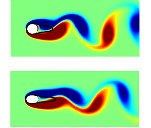
That being said, it is interesting to note that the mean drag coefficient of the optimal cylinders remains almost the same at all the noise levels (figure 8b), especially given that the shape of the optimised cylinder changes very little with the upstream noise level. Table 2 further reports the mean drag coefficients and the standard deviation for the circular cylinder and the cylinders optimised at different noise levels. In fact, similarly to the optimised cylinder, the mean drag coefficients of the circular cylinder barely change with an elevation of the upstream noise level, despite a significant increase in the standard deviations. This suggests that the upstream noise does not appear to have a significant influence on the flow around the cylinder itself. This is supported further in figure 9, where instantaneous snapshots of spanwise vorticity field are visualised for both circular and optimal cylinders with the mean recirculation zone. For both the circular and optimal cylinders, the sizes of the mean recirculation zones are almost identical, and the spanwise vorticity fields seem to be almost unaffected by two different noise levels $\sigma /\bar {U} = 0$ and $\sigma /\bar {U} = 0.01$. In fact, the only notable feature in figure 9 is that the vortex shedding in the optimal cylinder wake (figures 9b,d) is weaker than that in the circular cylinder (figures 9a,c) regardless of the noise level, consistent with the increased length of the recirculation zone in the optimal cylinder wakes.

Figure 9. Instantaneous vorticity field and the time-averaged recirculation zone for (a,c) the circular cylinder, and (b,d) the optimal cylinder: (a,b) $\sigma /\bar {U} = 0$; (c,d) $\sigma /\bar {U} = 0.01$. Here, the thick solid line indicates the isocontour of $\bar {u}=0$.

Table 2. Mean drag coefficient and standard deviation of the circular and optimal cylinders for different noise levels.

The insensitive nature of many flow properties observed in the present study is reminiscent of the early discussion on the cylinder wake in terms of oscillator versus noise amplifier (see e.g. Huerre & Monkewitz 1990; Chomaz 2005). The cylinder wake at $Re=100$ is an oscillator flow, in which external noise is known to play a limited role in the linear evolution of the instability related to vortex shedding. While the noise-insensitive nature of the flow properties observed in the present study might well be viewed as typical behaviours of the oscillator flow, we note that the classification of a flow in terms of oscillator versus noise amplifier was made based on a linear stability theory. In contrast, the insensitive flow properties discussed in this study are ‘time-averaged ones’ of ‘fully nonlinear’ vortex shedding. Furthermore, the original discussion on the noise insensitivity of oscillator flows in Huerre & Monkewitz (1990) was on the ill-posedness of the solution to the classical linear signalling problem (Huerre & Monkewitz 1985) in absolutely or globally unstable flows rather than on the effect of external noise in the fully nonlinear regime.

Therefore, to clarify these observations further, we perform a perturbation analysis. Given that the standard deviation of the imposed upstream noise is sufficiently small (less than 1 % of $\bar {U}$), the flow at the inlet boundary may be written as $u|_{\partial \varOmega _{{inlet}}} =1+\epsilon \,U_1(t)/\bar {U}$, where $U_1(t)=(U(t)/\bar {U}-1)/\epsilon$, with $\epsilon \sim O(\sigma /\bar {U}) \ll 1$. This allows the velocity and pressure fields to be expanded as $\boldsymbol {u}(t,x,y)=\boldsymbol {u}_0(t,x,y)+\epsilon \,\boldsymbol {u}_1(t,x,y)+O(\epsilon ^2)$ and $p(t,x,y)=p_0(t,x,y)+\epsilon \,p_1(t,x,y)+O(\epsilon ^2)$. Then the following equations of motion are obtained at $O(1)$:

(3.2a)\begin{equation} \frac{\partial \boldsymbol{u}_0}{\partial t}=\mathcal{NS}(\boldsymbol{u}_0,p_0), \end{equation}

with

(3.2b)\begin{equation} u_0|_{\partial \varOmega_{{inlet}}} =1, \end{equation}

where $\mathcal {NS}$ is the Navier–Stokes operator. At the next order (i.e. $O(\epsilon )$),

(3.3a)\begin{equation} \frac{\partial \boldsymbol{u}_1}{\partial t}=\frac{\partial \mathcal{NS}}{\partial \boldsymbol{u}}\bigg|_{\boldsymbol{u}_0}[\boldsymbol{u}_1\ p_1]^{\rm T}, \end{equation}

with

(3.3b)\begin{equation} u_1|_{\partial \varOmega_{{inlet}}} =U_1(t) \end{equation}

where ${\partial \mathcal {NS}/\partial \boldsymbol {u}}|_{\boldsymbol {u}_0}$ is the linearised Navier–Stokes operator about ${\boldsymbol {u}_0}$. We note that this operator should be stable in the two-dimensional wake at $Re=100$, as the first three-dimensional instability appears at a considerably higher Reynolds number (see e.g. Barkley & Henderson 1996; Williamson 1996). Therefore, (3.3) provides a well-posed (non-blowing-up) solution with $\boldsymbol {u}_1 \sim O(1)$ and $p_1 \sim O(1)$ from the driving mechanism imposed in (3.3b).

The analysis above now suggests that the flow field at the leading order is identical to that without noise, and the difference caused by the upstream noise is expected to remain at $O(\epsilon )$. This is consistent with the time trace of $C_L(t)$ in figure 7(a) and the snapshots of the spanwise vorticity reported in figure 9. However, this is not the case for the instantaneous drag given by

(3.4)\begin{equation} C_D(t)=C_D(\boldsymbol{u}_0,p_0)+\epsilon\,C_D(\boldsymbol{u}_1,p_1)+\cdots, \end{equation}

where $C_D(\boldsymbol {u},p)$ is the drag coefficient obtained using (2.14). As discussed already, $C_D(\boldsymbol {u}_1,p_1) \sim \Delta t^{-1}$ due to the effect of added mass. Therefore, even for a small noise level resulting in $\epsilon \ (\sim O(\sigma /\bar {U})) \sim \Delta t$, the fluctuations in $C_D(\boldsymbol {u}_1,p_1)$ become $O(\epsilon ^{-1})$ and cannot be ignored due to the added mass effect – note that this is the case of figure 7(a) where $\epsilon \sim 0.01$ and $\Delta t=0.01$. Nevertheless, it is important to note that the objective functional in the present study is a time-averaged quantity. Given that $C_D(\boldsymbol {u},p)$ is a linear functional of $\boldsymbol {u}$ and $p$, we have $\overline{C_D}(\boldsymbol {u}_1,p_1)={C}_D(\bar {\boldsymbol {u}}_1,\bar {p}_1)$. Also, since $\boldsymbol {u}_1$ and $p_1$ are of order unity, so are $\bar {\boldsymbol {u}}_1$ and $\bar {p}_1$, resulting in $\overline{C_D}(\boldsymbol {u}_1,p_1) \sim O(1)$. Therefore, the time-averaged drag $\overline{C_D}$, the objective functional in this study, would be affected at most by the size of the small upstream noise considered, i.e.

(3.5)\begin{equation} \overline{C_D}(\boldsymbol{u},p)=\overline{C_D}(\boldsymbol{u}_0,p_0)+O(\epsilon), \end{equation}

consistent with the values of $\overline{C_D}$ reported in table 2. This also explains why the optimal cylinder shapes obtained for the different noise levels are almost unchanged (figure 8a), despite the large fluctuations in $C_D(t)$, especially for the highest level of upstream noise considered (see figure 8(b) for $\sigma /\bar {U}=0.01$).

3.3. Drag reduction mechanism

Finally, we discuss briefly the drag reduction mechanism by which the optimal geometry is able to reduce the mean drag. Table 3 reports the breakdown of the drag of the optimal cylinder into the pressure and viscous components, and it is compared with that of the circular cylinder retaining the same area. Here, the noise level reported is $\sigma /\bar {U}=0.01$, and the result in table 3 changes little for the different noise levels considered in this study, as discussed above. It is seen that the drag reduction originates mainly from the reduction in the pressure drag component, consistent with the considerably weakened vortex shedding observed in the optimal cylinder wake (see figure 9). On the contrary, the optimal cylinder exhibits an elevated viscous drag compared to the circular cylinder, and this is because the optimal cylinder is more slender than the circular cylinder, while retaining the same internal area. However, the amount of the elevated viscous drag is quite small, as it is only approximately 1 % of the total drag of the circular cylinder. This implies that the optimal cylinder minimises the increase of the viscous drag, while it significantly reduces the pressure drag more directly related to the vortex shedding in the wake.

Table 3. Mean drag coefficient and standard deviation of circular and optimal cylinders for $\sigma /\bar {U} = 0.01$. Here, the subscripts $\nu$ and $p$ refer to the viscous and pressure components of the drag coefficient, respectively.

To better understand the reduced pressure drag of the optimal cylinder, figure 10 reports the time-averaged surface pressure distribution of the circular cylinder and the optimal cylinder with/without the upstream noise. As expected from the analysis in § 3.2, the noise affects the time-averaged pressure very little. The optimal cylinder exhibits a smaller pressure drop than the circular cylinder in the region where the near-wall flow would be accelerated ($120^\circ \lesssim \theta \leq 180^\circ$), and its base region ($\theta \simeq 0^\circ$) has higher pressure recovery than that of the circular cylinder, exhibiting a pressure drag reduction.

Figure 10. Time-averaged pressure distribution over the azimuthal angle $\theta$ at the cylinder surface at $Re=100$, for (a) $\sigma /\bar {U}=0$, (b) $\sigma =0.01/\bar {U}$, for the cases with stochastic noise. The pressure is normalised by its value near the stagnation point ($\theta =0^\circ$) that is identical in all the cases.

3.4. Effect of Reynolds number

The effect of the Reynolds number is explored finally by considering further $Re=150,200$. We note that the three-dimensional instability of vortex shedding takes place for $Re\gtrsim 188$ for the circular cylinder (Barkley & Henderson 1996; Williamson 1996). Here, this effect is suppressed artificially by performing two-dimensional flow simulations. The shape optimisation for three-dimensional turbulent flows is possible if enough computational resource is available, but this is beyond the scope of the present study. Instead, here we mainly explore the effect of inertial force in the given fluid flow by increasing the Reynolds number.

Figure 11 reports two optimal shapes found for $Re \geq 150$: one is the global minimiser of the objective functional (figure 11a), and the other is a local minimiser (i.e. suboptimum; figure 11b). We note that the suboptimal shapes obtained at $Re=150,200$ have been tested as initial conditions for the given optimisation algorithm at $Re=100$ to check if there exist similar suboptimal shapes at that Reynolds number. However, the optimisation yields the shape identical to the global minimiser found in § 3.1, suggesting that such a suboptimal shape is unlikely to exist at $Re=100$. The other interesting feature of the suboptimal shapes is that they retain smaller $\overline{C_D}$, while having slightly larger values of the objective functional: for example, $J=1.1671$ and $\overline{C_D}=0.9769$ for the global optimum, and $J=1.2444$ and $\overline{C_D}=0.9689$ for the suboptimum at $Re=200$. Indeed, the suboptimal shape at $Re=200$ exhibits a relatively slender base, reminiscent of an aerofoil. This suggests that the aerofoil-like suboptimal shape is likely the effect of inertial force (i.e. high Reynolds number), and it also implies that a delicate formulation of the optimisation constraints may yield this aerofoil-like suboptimal shape as the global optimum.

Figure 11. Effect of Reynolds number on the optimal cylinder geometry ($\sigma =0.01/\bar {U}$, $\lambda =10$, $N=35$): (a) global optimum; (b) suboptimum.

4. Conclusions

In the present study, the shape of a two-dimensional cylinder in a noisy laminar flow has been optimised to minimise its time-averaged drag. The noise is implemented by a small inline stochastic oscillation of the free-stream velocity obeying the Ornstein–Uhlenbeck process, and it leads to a large random fluctuation of instantaneous drag due to the effect of added mass. Under such a strong random fluctuation of drag, a shape optimisation is formulated using an ensemble-variation-based method (EnVar) to bypass the difficulty that the conventional adjoint-based optimisation faces in this problem. The geometry has been parametrised using a Fourier series, and the optimisation problem is formulated subject to an equality constraint imposing the same internal area and an inequality constraint limiting its streamwise length. Furthermore, to ensure a sufficiently smooth cylinder surface, a Tikhonov regularisation is implemented on the objective functional. It is found that the optimised cylinder geometry is close to a nearly symmetric slender oval at $Re=100$. As $Re$ is increased, two optimal shapes are found: one is identical to the oval shape obtained at $Re=100$, and the other is an asymmetric oval, the rear side of which is more slender than the front side, like an aerofoil. Despite the large random fluctuation in drag due to the added-mass effect, the optimal cylinder shapes obtained for different levels of upstream noise are found to be almost identical. Using a perturbation analysis, it is further shown that this robust nature of the optimal cylinder shape to the upstream noise is associated with the limited influence of the small upstream noise on the mean flow properties of the cylinder wake. Finally, the optimal cylinder is found to primarily reduce pressure drag associated mainly with vortex shedding in the wake. This comes at a cost of marginally increasing the viscous drag associated with the shape change.

It is finally worth mentioning that the EnVar used in this study is particularly useful for the optimisation in the presence of unknown biased noise and/or turbulence, which prevent the utilisation of the well-established adjoint-based method. However, this comes at a large computational cost – the adjoint-based optimisation requires only single run of direct and adjoint simulations to evaluate the gradient of an arbitrary objective functional, whereas the EnVar requires a number of direct simulations comparable to the degrees of freedom of the objective functional. Hence, because of a methodological element, the EnVar is computationally more expensive than the adjoint-based approach, although the adjoint-based approach may require large computer memory to store the full flow field information in time and space – typically rectified by applying a checkpoint algorithm. The key success in the application of the EnVar would therefore lie in how one would effectively approximate the gradient of the given objective functional by minimising the number of direct simulations, and this will be an important issue to study in the future.

References

Abergel, F. & Temam, R. 1990 On some control problems in fluid mechanics. Theor. Comput. Fluid Dyn. 1 (6), 303325.CrossRefGoogle Scholar
Arcas, D. & Redekopp, L. 2004 Aspects of wake vortex control through base blowing/suction. Phys. Fluids 16, 452456.Google Scholar
Baek, S. & Sung, H.J. 1998 Numerical simulation of the flow behind a rotary oscillating circular cylinder. Phys. Fluids 10, 869876.CrossRefGoogle Scholar
Barkley, D. & Henderson, R.D. 1996 Three-dimensional Floquet stability analysis of the wake of a circular cylinder. J. Fluid Mech. 322, 215241.CrossRefGoogle Scholar
Bearman, P.W. 1965 Investigation of the flow behind a two-dimensional model with a blunt trailing edge and fitted with splitter plates. J. Fluid Mech. 21, 241255.CrossRefGoogle Scholar
Bearman, P.W. 1967 The effect of base bleed on the flow behind a two-dimensional model with a blunt trailing edge. Aeronaut. Q. 18, 207224.CrossRefGoogle Scholar
Bearman, P.W. & Owen, J.C. 1998 Reduction of bluff-body drag and suppression of vortex shedding by the introduction of wavy separation lines. J. Fluids Struct. 12, 123130.CrossRefGoogle Scholar
Bewley, T.R., Moin, P. & Temam, R. 2001 DNS-based predictive control of turbulence: an optimal benchmark for feedback algorithms. J. Fluid Mech. 447, 179225.CrossRefGoogle Scholar
Blackburn, H. & Henderson, R. 1999 A study of two-dimensional flow past an oscillating cylinder. J. Fluid Mech. 385, 255286.CrossRefGoogle Scholar
Blanchard, A., Bergman, L.A. & Vakakis, A.F. 2020 Vortex-induced vibration of a linearly sprung cylinder with an internal rotational nonlinear energy sink in turbulent flow. Nonlinear Dyn. 99 (1), 593609.CrossRefGoogle Scholar
Brewster, J. & Juniper, M. 2020 Shape sensitivity of eigenvalues in hydrodynamic stability, with physical interpretation for the flow around a cylinder. Eur. J. Mech. (B/Fluids) 80, 8091.Google Scholar
Choi, H., Jeon, W.-P. & Kim, J. 2008 Control of flow over a bluff body. Annu. Rev. Fluid Mech. 40, 113139.CrossRefGoogle Scholar
Choi, S., Choi, H. & Kang, S. 2002 Characteristics of flow over a rotationally oscillating cylinder at low Reynolds number. Phys. Fluids 140, 27672777.CrossRefGoogle Scholar
Chomaz, J.M. 2005 Global instabilities in spatially developing flows: nonnormality and nonlinearity. Annu. Rev. Fluid Mech. 37, 357392.CrossRefGoogle Scholar
Colburn, C.H., Cessna, J.B. & Bewley, T.R. 2011 State estimation in wall-bounded flow systems. Part 3. The ensemble Kalman filter. J. Fluid Mech. 682, 289303.CrossRefGoogle Scholar
Darekar, R.M. & Sherwin, S.J. 2001 Flow past a square-section cylinder with a wavy stagnation face. J. Fluid Mech. 426, 263295.CrossRefGoogle Scholar
Evensen, G. 2009 Data Assimilation: The Ensemble Kalman Filter. Springer.CrossRefGoogle Scholar
Giannetti, F. & Luchini, F. 2007 Structural sensitivity of the first instability of the cylinder wake. J. Fluid Mech. 581, 167197.CrossRefGoogle Scholar
Hecht, F. 2012 New development in FreeFem++. J. Numer. Maths 20 (3–4), 251265.Google Scholar
Huerre, P. & Monkewitz, P.A. 1985 Absolute and convective instabilities in free shear layers. J. Fluid Mech. 159, 151168.CrossRefGoogle Scholar
Huerre, P. & Monkewitz, P.A. 1990 Local and global instabilities in spatially developing flows. Annu. Rev. Fluid Mech. 22, 473537.CrossRefGoogle Scholar
Jahanbakhshi, R. & Zaki, T.A. 2019 Nonlinearly most dangerous disturbance for high-speed boundary-layer transition. J. Fluid Mech. 876, 87121.CrossRefGoogle Scholar
Kato, H., Yoshizawa, A., Ueno, G. & Obayashi, S. 2015 A data assimilation methodology for reconstructing turbulent flows around aircraft. J. Comput. Phys. 283, 559581.CrossRefGoogle Scholar
Kwon, K. & Choi, H. 1996 Control of laminar vortex shedding behind a circular cylinder using splitter plates. Phys. Fluids 8, 478496.CrossRefGoogle Scholar
Lasagna, D. 2018 Sensitivity analysis of chaotic systems using unstable periodic orbits. SIAM J. Appl. Dyn. Sys. 17 (1), 547580.CrossRefGoogle Scholar
Lasagna, D., Sharma, A. & Meyers, J. 2019 Periodic shadowing sensitivity analysis of chaotic systems. J. Comput. Phys. 391, 119141.CrossRefGoogle Scholar
Lewis, J.M., Lakshmivarahan, S. & Dhall, S.K. 2006 Dynamic Data Assimilation: A Least Squares Approach. Cambridge University Press.CrossRefGoogle Scholar
Lim, S. & Choi, H. 2004 Optimal shape design of a two-dimensional asymmetric diffuser in turbulent flow. AIAA J. 42 (6), 11541169.Google Scholar
Mao, X., Blackburn, H.M. & Sherwin, S.J. 2015 Nonlinear optimal suppression of vortex shedding from a circular cylinder. J. Fluid Mech. 775, 241265.CrossRefGoogle Scholar
Marensi, E., Willis, A.P. & Kerswell, R.R. 2020 Designing a minimal baffle to destabilise turbulence in pipe flows. J. Fluid Mech. 900, A31.CrossRefGoogle Scholar
Marquet, O., Sipp, D. & Jacquin, L. 2008 Sensitivity analysis and passive control of cylinder flow. J. Fluid Mech. 615, 221252.CrossRefGoogle Scholar
Min, C. & Choi, H. 1999 Suboptimal feedback control of vortex shedding at low Reynolds numbers. J. Fluid Mech. 401, 123156.Google Scholar
Mohammadi, B. & Pironneau, O. 2009 Applied Shape Optimization for Fluids. Oxford Scholarship Online.CrossRefGoogle Scholar
Mohan, P., Fitzsimmons, N. & Moser, R.D. 2017 Scaling of Lyapunov exponents in homogeneous isotropic turbulence. Phys. Rev. Fluids 2 (11), 114606.CrossRefGoogle Scholar
Mons, V., Chassaing, J.-C., Gomez, T. & Sagaut, P. 2016 Reconstruction of unsteady viscous flows using data assimilation schemes. J. Comput. Phys. 316, 255280.CrossRefGoogle Scholar
Mons, V., Du, Y. & Zaki, T.A. 2021 Ensemble-variational assimilation of statistical data in large-eddy simulation. Phys. Rev. Fluids 6, 104607.CrossRefGoogle Scholar
Ni, A., Wang, Q., Fernandez, P. & Talnikar, C. 2019 Sensitivity analysis on chaotic dynamical systems by finite difference non-intrusive least squares shadowing (FD-NILSS). J. Comput. Phys. 394, 615631.CrossRefGoogle Scholar
Nocedal, J. & Wright, S.J. 2006 Numerical Optimization, 2nd edn. Springer.Google Scholar
Park, H., Jeon, W.-P., Choi, H. & Yoo, J.Y. 2006 Drag reduction in flow over a two-dimensional bluff body with a blunt trailing edge using a new passive device. J. Fluid Mech. 563, 389414.CrossRefGoogle Scholar
Pironneau, O. 1974 On optimum design in fluid mechanics. J. Fluid Mech. 64, 97110.CrossRefGoogle Scholar
Roshko, A. 1955 On the wake and drag of bluff bodies. J. Aeronaut. Sci. 22, 12.Google Scholar
Spall, J.C. 2003 Introduction to Stochastic Search and Optimization: Estimation, Simulation and Control. Wiley.CrossRefGoogle Scholar
Strykowski, P.J. & Sreenivasan, K.R. 1990 On the formation and suppression of vortex ‘shedding’ at low Reynolds number. J. Fluid Mech. 218, 71107.CrossRefGoogle Scholar
Suzuki, T. 2012 Reduced-order Kalman-filtered hybrid simulation combining particle tracking velocimetry and direct numerical simulation. J. Fluid Mech. 705, 249288.CrossRefGoogle Scholar
Tokumaru, P.T. & Dimotakis, P.E. 1991 Rotary oscillation control of a cylinder wake. J. Fluid Mech. 224, 7790.CrossRefGoogle Scholar
Tombazis, N. & Bearman, P.W. 1997 A study of three dimensional aspects of vortex shedding from a bluff body with a mild geometric disturbance. J. Fluid Mech. 330, 85112.CrossRefGoogle Scholar
Wang, Q., Hu, R. & Blonigan, P. 2014 Least squares shadowing sensitivity analysis of chaotic limit cycle oscillations. J. Comput. Phys. 267, 210224.CrossRefGoogle Scholar
Williamson, C.H.K. 1996 Vortex dynamics in the cylinder wake. Annu. Rev. Fluid Mech. 28, 477539.CrossRefGoogle Scholar
Wood, C.J. 1967 The effect of base bleed on a periodic wake. J. Aeronaut. Soc. 68, 477482.CrossRefGoogle Scholar
Wright, S. & Nocedal, J. 1999 Numerical optimization. Springer Sci. 35 (67–68), 7.Google Scholar
Yang, Y., Robinson, C., Heitz, D. & Mémin, E. 2015 Enhanced ensemble-based 4DVar scheme for data assimilation. Comput. Fluids 115, 201210.CrossRefGoogle Scholar
Zhou, K., Doyle, J.C. & Glover, K. 1996 Robust and Optimal Control. Prentice Hall.Google Scholar