Hostname: page-component-cd9895bd7-gvvz8 Total loading time: 0 Render date: 2024-12-25T19:35:20.204Z Has data issue: false hasContentIssue false

Transformer-based in-context policy learning for efficient active flow control across various airfoils

Published online by Cambridge University Press:  19 December 2024

Changdong Zheng
Affiliation:
Center for Engineering and Scientific Computation, Zhejiang University, Zhejiang 310027, PR China
Fangfang Xie*
Affiliation:
Center for Engineering and Scientific Computation, Zhejiang University, Zhejiang 310027, PR China
Tingwei Ji
Affiliation:
Center for Engineering and Scientific Computation, Zhejiang University, Zhejiang 310027, PR China
Hongjie Zhou
Affiliation:
Center for Engineering and Scientific Computation, Zhejiang University, Zhejiang 310027, PR China
Yao Zheng
Affiliation:
Center for Engineering and Scientific Computation, Zhejiang University, Zhejiang 310027, PR China
*
Email address for correspondence: fangfang_xie@zju.edu.cn

Abstract

Active flow control based on reinforcement learning has received much attention in recent years. Indeed, the requirement for substantial data for trial-and-error in reinforcement learning policies has posed a significant impediment to their practical application, which also serves as a limiting factor in the training of cross-case agents. This study proposes an in-context active flow control policy learning framework grounded in reinforcement learning data. A transformer-based policy improvement operator is set up to model the process of reinforcement learning as a causal sequence and autoregressively give actions with sufficiently long context on new unseen cases. In flow separation problems, this framework demonstrates the capability to successfully learn and apply efficient flow control strategies across various airfoil configurations. Compared with general reinforcement learning, this learning mode without the need for updating the network parameter has even higher efficiency. This study presents an effective novel technique in using a single transformer model to address the flow separation active flow control problem on different airfoils. Additionally, the study provides an innovative demonstration of incorporating reinforcement-learning-based flow control with aerodynamic shape optimization, leading to collective enhancement in performance. This method efficiently lessens the training burden of the new flow control policy during shape optimization, and opens up a promising avenue for interdisciplinary intelligent co-design of future vehicles.

Type
JFM Papers
Copyright
© The Author(s), 2024. Published by Cambridge University Press

1. Introduction

For a long time, improving aerodynamic performance has consistently stood as a critical objective for aeronautical researchers and manufacturers. The pursuit of this goal is driven by various factors, including economic benefits, energy conservation and military requirements. Consequently, there has been a substantial focus on advancing aerodynamic capabilities, leading to the development of technologies such as aerodynamic shape optimization (Jameson Reference Jameson2003; Li, Du & Martins Reference Li, Du and Martins2022) and active flow control (Collis et al. Reference Collis, Joslin, Seifert and Theofilis2004; Choi, Jeon & Kim Reference Choi, Jeon and Kim2008). Typically, these technologies are dealt with separately due to the inherent complexity of finding effective solutions for their specific challenges. The intricate nature of these problems demands focused attention, acknowledging the multifaceted aspects involved to achieve superior aerodynamic performance.

Active flow control (AFC) emerges as a promising area of research where actuators (Cattafesta & Sheplak Reference Cattafesta and Sheplak2011), such as mass jets and fluidic vortex generators, are commonly installed on vehicle surfaces to induce controlled disturbances in the flow. Control laws, or policies, can be adaptively specified to address diverse objectives, ranging from separation delays (Greenblatt & Wygnanski Reference Greenblatt and Wygnanski2000) to vibration eliminations (Yao & Jaiman Reference Yao and Jaiman2017; Zheng et al. Reference Zheng, Ji, Xie, Zhang, Zheng and Zheng2021). However, devising efficient control policies demands substantial effort, given the complex challenge of precisely modelling high-dimensional nonlinear flow systems (Choi et al. Reference Choi, Temam, Moin and Kim1993; Lee, Kim & Choi Reference Lee, Kim and Choi1998; Gao et al. Reference Gao, Zhang, Kou, Liu and Ye2017; Deem et al. Reference Deem, Cattafesta, Hemati, Zhang, Rowley and Mittal2020). In recent times, reinforcement learning, as a model-free control method, has gained growing attention in the field of fluid mechanics (Gazzola, Hejazialhosseini & Koumoutsakos Reference Gazzola, Hejazialhosseini and Koumoutsakos2014; Reddy et al. Reference Reddy, Wong-Ng, Celani, Sejnowski and Vergassola2018; Verma, Novati & Koumoutsakos Reference Verma, Novati and Koumoutsakos2018; Yan et al. Reference Yan, Chang, Tian, Wang, Zhang and Liu2020). Within the AFC domain, Rabault et al. (Reference Rabault, Kuchta, Jensen, Réglade and Cerardi2019) showcased a successful demonstration of cylinder-drag reduction through a computational fluid dynamics (CFD) simulation employing an artificial neural network. This demonstration established a control policy from velocity probes to control mass jets. Similarly, Fan et al. (Reference Fan, Yang, Wang, Triantafyllou and Karniadakis2020) illustrated the effectiveness of reinforcement learning in experimental settings, specifically for drag reduction. In larger scale high-fidelity three-dimensional (3-D) simulations, such as channel flow, Guastoni et al. (Reference Guastoni, Rabault, Schlatter, Azizpour and Vinuesa2023) and Sonoda et al. (Reference Sonoda, Liu, Itoh and Hasegawa2023) each proposed their own novel reinforcement learning flow control solutions for drag reduction, further advancing our understanding of complex, turbulent physical systems. Each passing year witnesses the publication of numerous related works, showing researchers actively tapping into the potential of reinforcement learning in AFC (Rabault et al. Reference Rabault, Ren, Zhang, Tang and Xu2020; Garnier et al. Reference Garnier, Viquerat, Rabault, Larcher, Kuhnle and Hachem2021; Vignon, Rabault & Vinuesa Reference Vignon, Rabault and Vinuesa2023b; Xie et al. Reference Xie, Zheng, Ji, Zhang, Bi, Zhou and Zheng2023).

Reinforcement learning, being an interactive data-driven method, exhibits a substantial demand for data (Botvinick et al. Reference Botvinick, Ritter, Wang, Kurth-Nelson, Blundell and Hassabis2019; Zheng et al. Reference Zheng, Xie, Ji, Zhang, Lu, Zhou and Zheng2022). The costs associated with acquiring flow data and the lengthy training times, particularly when compared with more common applications such as video games (Shao et al. Reference Shao, Tang, Zhu, Li and Zhao2019), have limited the widespread adoption of this algorithm. However, there are related studies, such as those focusing on parallelization across multi-environments (Rabault et al. Reference Rabault, Ren, Zhang, Tang and Xu2020) and transferring policies from coarse-mesh cases to finer-mesh cases (Ren, Rabault & Tang Reference Ren, Rabault and Tang2021), that have demonstrated significant acceleration effects on single cases. Consequently, another innovative approach involves identifying and extracting correlations between similar problems, which enables rapid adaptation without having to restart the learning process from scratch with each iteration. Transfer learning, a method involving the transfer of parameters from source domains to target domains, has proven effective and is widely employed in various domains, including fluid dynamics (Konishi, Inubushi & Goto Reference Konishi, Inubushi and Goto2022; Wang et al. Reference Wang, Hua, Aubry, Chen, Wu and Cui2022). More directly, Tang et al. (Reference Tang, Rabault, Kuhnle, Wang and Wang2020) trains a robust flow control agent over a range of Reynolds numbers, i.e. 100, 200, 300, 400, which can also effectively reduce drag for any previously unseen value of the Reynolds number between 60 and 400. However, when there exists a significant divergence in data distribution and features between the source and target domains, the policy in the source domain may be invalid and require substantial adjustments bringing higher training costs. This challenge is particularly pronounced in aircraft design (Raymer Reference Raymer2012), a domain characterized by iterative processes that span the entire design cycle. The significant distinctions between first-generation and final-generation prototypes impose increased demands on the effective adaptation and performance improvement of AFC.

To tackle the challenges, researchers advocate using transformers, recognized for their ability to adeptly manage extensive sequences and contextual information through attention mechanisms (Vaswani et al. Reference Vaswani, Shazeer, Parmar, Uszkoreit, Jones, Gomez, Kaiser and Polosukhin2017). Transformers have proven successful across various AI domains, including natural language processing (Wolf et al. Reference Wolf2020) and computer vision (Han et al. Reference Han2022). In the field of fluid mechanics, Wang et al. (Reference Wang, Lin, Zhao, Chen, Guo, Yang, Wang and Fan2024) uses the transformer architecture to model the time-dependent behaviour of partially observable flapping airfoils, achieving enhanced performance compared with approaches using recurrent neural networks or multilayer perceptrons. For reinforcement learning, transformers are increasingly employed in in-context learning (Dong et al. Reference Dong, Li, Dai, Zheng, Wu, Chang, Sun, Xu and Sui2022; Min et al. Reference Min, Lyu, Holtzman, Artetxe, Lewis, Hajishirzi and Zettlemoyer2022), where the model leverages previously observed sequences as context to infer optimal actions without the need for explicit parameter updates. This reframes the Markov decision process as a sequence modelling challenge, aiming to generate action sequences that yield substantial rewards when executed in a given environment (Chen et al. Reference Chen, Lu, Rajeswaran, Lee, Grover, Laskin, Abbeel, Srinivas and Mordatch2021; Janner, Li & Levine Reference Janner, Li and Levine2021).

Meanwhile, a new paradigm for policy learning across multiple cases has emerged, involving policy extraction from extensive datasets encompassing sequence data from diverse domains (Lee et al. Reference Lee2022; Reed et al. Reference Reed2022). Notably, Laskin et al. (Reference Laskin2022) proposes transformers as policy improvement operators in environments with sparse rewards, combinatorial case structures and pixel-based observations. Their algorithm distillation technique incrementally enhances policies for new cases through in-context interactions with the environment, meaning the model adapts to new situations based on past experiences without requiring additional training. This approach offers meaningful insights for reinforcement-learning-based active flow control, especially in highly repeatable domains like aircraft design, where the model can efficiently apply learned control strategies across varying airfoil configurations.

In this study, it is the first time that the algorithm distillation is introduced to enhance reinforcement learning-based AFC challenges. Leveraging a transformer model, we formulate the reinforcement learning sequence and predict actions autoregressively, using learning histories as contextual information. This model acts as an in-context policy improvement operator, gradually refining policies as long as the contextual information spans a sufficient duration. We establish an in-context AFC policy learning framework grounded in this policy improvement operator, encompassing three key stages: data collection, offline training and online evaluation. We have prepared a low-Reynolds-number airfoil flow separation system to assess the efficiency of this framework. It demonstrates that the transformer neural network can learn closed-loop AFC policy improvement operators, which is exactly the same as a general reinforcement learning algorithm except the learning happens without updating the network parameters. One machine learning model can be used to address different active flow control cases. Finally, this study showcases how to integrate an in-context active flow control policy learning framework with aerodynamic shape optimization to jointly enhance performance. Moreover, the research showcases an innovative approach by integrating reinforcement-learning-based flow control with aerodynamic shape optimization, resulting in a notable improvement in performance.

The remainder of this paper is organized as follows: § 2 introduces the methods mainly used in our framework; § 3 provides an overview of the environment configuration considered in this study; the results are detailed in § 4; and finally, we summarize our key conclusions and prospect our future work in § 5.

2. Methodology

This section introduces a new in-context AFC policy learning framework using a policy improvement operator. The flow chart of this method is depicted in figure 1, outlining three stages: data collection, offline training and online evaluation. In the first stage, reinforcement learning agents generate learning data for various cases. Subsequently, a policy improvement operator is established to model reinforcement learning as a causal sequence prediction problem. The concept of algorithm distillation supports the learning of policy improvement operators. During the online evaluation stage, the trained agent interacts with the environment autoregressively, enhancing the AFC policy only in-context. A comprehensive overview of the entire framework is provided in § 2.4.

Figure 1. Whole architecture of the active flow control policy learning framework via policy improvement operator.

2.1. Reinforcement learning

Reinforcement learning (Sutton & Barto Reference Sutton and Barto2018) is the policy optimization algorithm that furnishes process data for policy improvement during the data collection stage. This algorithm addresses flow control problems as Markov decision processes (MDPs). The environment (flow system) evolves from the state $s_t$ to the next state $s_{t+1}$ based on action $a_t$ and provides feedback reward $r_t$ to the agent, modelled as

(2.1)\begin{equation} x_{t+1} = f(x_t, a_t),\quad t=0,1,2,3,\ldots, \end{equation}

where $x_t=[s_t, r_t]$. In the context of reinforcement learning, the objective is to find an optimal policy ${\rm \pi} ^*$ that dictates which action to take in this MDP. The cost function $J$ is equivalent to the expected value of the discounted sum of rewards for a given policy ${\rm \pi} $, defined as

(2.2)\begin{equation} J({\rm \pi} ) = E_{\tau \sim {\rm \pi}}\left[\sum_{t=0}^{T} \gamma^t r_t\right],\end{equation}

where $T$ marks the end of an episode and $\tau =(s_0, a_0, r_0, s_1, a_1, r_1, s_2, \ldots )$ is closely tied to the policy ${\rm \pi} $. Here, $\gamma$ represents the reward discount factor for algorithm convergence. Each reinforcement learning algorithm follows a distinct optimization process for the objective function. Typically, the policy is represented by a parametrized function ${\rm \pi} _\theta$.

The proximal policy optimization (PPO) algorithm (Schulman et al. Reference Schulman, Wolski, Dhariwal, Radford and Klimov2017) is employed in the data collection stage for each individual agent. Drawing inspiration from policy gradient (Sutton et al. Reference Sutton, McAllester, Singh and Mansour1999) and trust region methods (Schulman et al. Reference Schulman, Levine, Abbeel, Jordan and Moritz2015), the PPO algorithm introduces a novel surrogate objective function, created through a linear approximation of the original objective. By dynamically constraining the magnitude of policy updates, the algorithm ensures that the outcomes of the subsequent update will consistently outperform the previous one. The loss function $L^{clip}(\theta )$ of the PPO algorithm is the following:

(2.3)\begin{equation} L^{clip}(\theta)=E_{{\rm \pi} _\theta}[\min (\rho(\theta)A^{{\rm \pi} _\theta}(s,a), clip(\rho(\theta),1-\epsilon, 1+\epsilon)A^{{\rm \pi} _\theta}(s,a))]. \end{equation}

Here, $\rho (\theta )={{\rm \pi} _\theta (a \mid s)}/{{\rm \pi} _{\theta _{old}}(a \mid s)}$ represents the probability ratio, $\epsilon$ is the clipping parameter and $A$ is the advantage function, estimating the additional future return at state $s$ compared with the mean. The optimization of this objective is carried out using stochastic gradient ascent on the data batch derived from environment interactions. A detailed mathematical introduction to the PPO method is available in Appendix A.

2.2. Transformer and self-attention

Vaswani et al. (Reference Vaswani, Shazeer, Parmar, Uszkoreit, Jones, Gomez, Kaiser and Polosukhin2017) introduced a pioneering neural network architecture for machine translation, relying exclusively on attention layers rather than recurrence. In essence, a transformer model follows an encoder-decoder structure. The model is auto-regressive at each step, incorporating previously generated symbols as additional input when generating the next. In this context, we elaborate on the encoder architecture, which constitutes our operator model.

The encoder model consists of a stack of $N$ identical layers, each comprising two main components: a multi-head self-attention block, followed by a position-wise feed-forward network. The multi-head self-attention block takes input, including query $Q$, key $K$ and value $V$ vectors, with dimensions $d_Q$, $d_K$ and $d_V$, respectively. The key-value pairs compute attention distribution and selectively extract information from the value $V$. The attention function is calculated as

(2.4)\begin{equation} Attention(Q, K, V)=softmax\left(\frac{QK^T}{\sqrt{d_K}}\right)V. \end{equation}

In the transformer, instead of performing a single attention function with $d$-dimensional $Q$, $K$ and $V$, these vectors are projected $h$ times (number of attention heads) with different learned linear projections to a smaller dimension $d_Q=d/h$, $d_K=d/h$ and $d_V=d/h$ respectively. The attention function is then applied in parallel on these projected queries, keys and values to yield $d_V$-dimensional output values. These outputs are concatenated and once again projected, resulting in the final $d$-dimensional values. The output of this multi-head attention block is

(2.5)$$\begin{gather} MultiHead(Q, K, V)=Concat(head_1,head_2,\ldots,head_h)W^o, \end{gather}$$
(2.6)$$\begin{gather}head_i=Attention(QW_i^Q, KW_i^K, VW_i^V), \end{gather}$$

where $W$ are projections matrices.

In this study, we use $N=4$ identical encoder layers, $d=128$ output dimensions and $h=4$ heads for both cases. Additionally, artificial neural networks with different shapes are employed to adapt to various case dimensions.

2.3. Algorithm distillation

Algorithm distillation, introduced by Laskin et al. (Reference Laskin2022), is an innovative method that integrates reinforcement learning (Sutton et al. Reference Sutton, McAllester, Singh and Mansour1999), offline policy distillation (Lee et al. Reference Lee2022; Reed et al. Reference Reed2022), in-context learning (Brown et al. Reference Brown2020) and more. The premise is that if a transformer's context is sufficiently long to encompass policy improvement resulting from learning updates, it should be able to represent not only a fixed policy but also a policy improvement operator by attending to states, actions and rewards from previous episodes. This study is inspired by this idea, which suggests that different flow control policies can also be obtained through an operator trained on reinforcement learning data.

Algorithm distillation consists of two primary components. First, it generates a large data buffer $D$ by preserving the training histories of a source reinforcement learning algorithm $P^{source}$ on numerous individual cases ${M_n}_{n=1}^N$:

(2.7)\begin{equation} D:=\{(s_0^{(n)},a_0^{(n)},r_0^{(n)},\ldots,s_T^{(n)},a_T^{(n)},r_T^{(n)})\sim P^{source}_{M_n}\}^N_{n=1}, \end{equation}

where $N$ is the number of cases for data generation. Then, the method distils the source algorithm's behaviour into a sequence model that maps long histories to probabilities over actions with a negative log likelihood (NLL) loss. A neural network models $P_\theta$ with parameters $\theta$ is trained by minimizing the following loss function:

(2.8)\begin{gather} L(\theta):={-}\sum_{n=1}^N\sum_{t=1}^{T-1}\log_{P_\theta} (A=h_{t-1}^{(n)}\,|\,s_0^{(n)},s_t^{(n)}), \end{gather}
(2.9)\begin{gather}h_{t-1}^{(n)}=(s_0^{(n)},a_0^{(n)},r_0^{(n)},\ldots,s_{t-1}^{(n)}, a_{t-1}^{(n)},r_{t-1}^{(n)}). \end{gather}

After the completion of training, the model undergoes evaluation to deduce the improved policy by predicting the actions based on the history of new cases.

2.4. In-context AFC policy learning framework

This section introduces the in-context AFC policy learning framework via the policy improvement operator, illustrated in figure 1. The framework comprises three stages: collecting data, offline training and online evaluation.

In the initial stage, a substantial data buffer is established, encompassing variations in cases arising from distinct system with different airfoils. Each case involves an individual reinforcement learning agent interacting with the numerical simulation environment and implementing control for a predefined target. The control policy undergoes iterative optimization using the PPO algorithm, and the learning histories are recorded. The data buffer compiles the entire reinforcement learning process, connecting all episodes sequentially for each case.

The second stage involves learning a policy improvement operator model on a transformer, as depicted in figure 2. In our work, this model $f$, parametrized by $\theta$, is designed with three components: embedding network $f_\theta ^{E}$, transformer network $f_\theta ^{T}$ and actor network $f_\theta ^{A}$. The embedding network is built with mapping the across-episodic histories to an embedded dynamical system, where the transition $(a_{t-1}, r_{t-1}, s_{t})$ corresponds to an embedded state $\xi _t$, denoted as

(2.10)\begin{equation} \xi_t = f_\theta^{E}(a_{t-1}, r_{t-1}, s_{t}). \end{equation}

The embedded representation sequence $\varXi _t = [\xi _{t-L}, \xi _{t-L+1},\ldots,\xi _{t}]$ of the physical system with position embedding is entered into the transformer network, which is a stack of four identical encoder layers. The details of the transformer have already been discussed earlier. The output $Z_t = [z_{t-L},z_{t-L+1},\ldots,z_{t}]$ of transformer encoder is denoted as

(2.11)\begin{equation} Z_t = f_\theta^{T}(\varXi_t). \end{equation}

In the end, the actor network, composed of three feed forward networks, decodes the $Z_t$ into predicted action sequences

(2.12)\begin{equation} A_t^{pred} = f_\theta^{A}(Z_t). \end{equation}

Our problem involves a continuous-space control problem, and we use root-mean-square errors as the loss function:

(2.13)\begin{equation} L(\theta)=\frac{1}{m}\sum_{i=1}^{m} \|{A_{t,i}^{truth}}-{A_{t,i}^{pred}}\|^2. \end{equation}

Here, $A_t^{truth}$ and $A_t^{pred}$ respectively represent the real and predicted action sequence, and $m$ represents the batch size.

Figure 2. Neural network architecture of policy improvement operator.

The final stage involves online evaluation. For instance, in an aerodynamic shape optimization where various new airfoils serve as intermediate prototypes, flow control configurations remain consistent across different cases, such as the positions of jets and probes. An empty context queue is initialized and filled with interaction transitions from the new environment. The context with the current state is input into the policy improvement operator model, and the history-conditioned action is returned. With further interactions, the sum of rewards is recorded, serving as an indicator that presents the improvement level achieved through reinforcement learning.

In this study, we also develop a framework for surrogate model modelling and aerodynamic shape optimization using Gaussian processes and Bayesian optimization methods (Frazier Reference Frazier2018; Schulz, Speekenbrink & Krause Reference Schulz, Speekenbrink and Krause2018). Additionally, the rapid exploration and learning of flow control policies on the newly generated airfoil shape is achieved, which provides an example for the combination of reinforcement-learning-based active flow control and aerodynamic shape optimization, as illustrated in § 4.2.

In this work, all the reinforcement learning models and the transformer policy improvement operators are developed using PyTorch, a widely used Python package for machine learning (Paszke et al. Reference Paszke2019).

In addition to addressing the flow separation problem on various airfoils, this flow control strategy exploration framework can be applied to other challenges as well. Appendix C includes a vortex-induced vibration system governed by the Ogink model (Ogink & Metrikine Reference Ogink and Metrikine2010), which is used to further validate the effectiveness of the control framework.

3. Environment configuration

This section outlines the configuration of the airflow separation flow control system (environment). It involves a numerical simulation of airfoil flow separation using computational fluid dynamics. The shape of the airfoil changes randomly, which means different boundary conditions for the flow, resulting in different vortex structures. These various cases brings challenges to the learning.

3.1. Numerical simulation for airfoil flow separation

Research on airfoil flow separation represents one of the fundamental challenges in aerodynamics. A well-designed flow separation control policy contributes to increased lift or reduced drag, leading to enhanced energy efficiency and improved manoeuvrability.

In our work, the active flow control policy is explored to improve the lift of the airfoil. As illustrated in figure 3, the airfoil is located at the position of ($x = 0$, $y = 0$), with a chord length of $L=1$ m. The computational domain is extended from $x = -30$ m at the inlet to $x = 30$ m at the outlet and from $y = -30$ m to $y = 30$ m in the cross-flow direction. The uniform inflow velocity is 1 m s$^{-1}$, and there is an angle of attack $\beta =20^{\circ }$ between the inflow and the chord of the airfoil. The Reynolds number $Re$, as an important dimensionless number to characterize the viscous effect of flow, is set to 1000 in this case.

Figure 3. Configuration of airfoil flow and active flow control.

We place 10 probes on the upper surface of the airfoil to capture pressure information, which serves as the reinforcement learning state. Three actuator jets are strategically positioned at $25\,\%$, $50\,\%$ and $75\,\%$ of the upper surface, each with a width of $5\,\%$. These jets feature a parabolic spatial velocity profile to ensure a seamless transition. The injected flow mass instantaneously sums to zero, eliminating storage requirements for turnover in practical applications. Each episode spans 20 seconds and is subdivided into 200 interaction steps.

In the present study, the incompressible Navier–Stokes equation and the continuity equation are considered to solve this fluid dynamic problem, written in integral form:

(3.1)\begin{gather} \frac{\partial}{\partial{t}}\int_{V}\rho v\, {\rm d} V + \int_{S}\rho vv \cdot n \, {\rm d} S = \int_{S}div \,T \cdot n \, {\rm d} S + \int_{V}\rho b \, {\rm d} V, \end{gather}
(3.2)\begin{gather}\frac{\partial}{\partial{t}}\int_{V}\rho v\, {\rm d} V + \int_{S}\rho v \cdot n \, {\rm d} S = 0. \end{gather}

Here, $\rho$ represents fluid density, $v$ is the fluid velocity, $S$ is the control volume (CV) surface with $n$ as the unit normal vector directed outwards, $V$ denotes the CV, $T$ stands for the tensor representing surface forces due to pressure and viscous stresses, and $b$ represents volumetric forces such as gravity. The finite volume method within the open-source OpenFOAM platform is employed to solve the problem. This method involves dividing the computational domain into discrete control volumes $CV$. By summing all the flux approximations and source terms, an algebraic equation is derived, relating the variable value at the CV-centre to the values at neighbouring CVs with which it shares common faces:

(3.3)\begin{equation} A_p \phi_p + \sum_k A_k \phi_{N_k} = q_p. \end{equation}

Here, $\phi$ represents a generic scalar quantity, and the index $k$ runs over all $CV$-faces. The coefficients $A_k$ typically include contributions from convection and diffusion fluxes, while $Q$ encompasses source terms and deferred corrections. The PIMPLE algorithm is adopted here to decouple the velocity and pressure equations through an iterative prediction and correction process. A brief introduction to the numerical validation of grid size and time step is provided in Appendix D.

In this environment, the control objective is set to maximize lift and minimize drag of the airfoil. Two dimensionless parameters, lift coefficient $C_l$ and drag coefficient $C_d$, are defined for the quantification as follows:

(3.4)\begin{gather} {C_l} = \frac{{\displaystyle \int_C {(\sigma \cdot n)} \cdot {e_l}\,{\rm d}S}}{{\dfrac{1}{2}\rho {{\bar U}^2}C}}, \end{gather}
(3.5)\begin{gather}{C_d} = \frac{{\displaystyle \int_C {(\sigma \cdot n)} \cdot {e_d}\,{\rm d}S}}{{\dfrac{1}{2}\rho {{\bar U}^2}C}}, \end{gather}

where $\sigma$ is the Cauchy stress tensor, $n$ is the unit vector normal to the outer airfoil surface, $S$ is the surface of the airfoil, $C$ is the chord length of the airfoil, $\rho$ is the volumetric mass density of the fluid, ${\bar U}$ is the velocity of the uniform flow, $e_d=(\sin \beta,\cos \beta )$ and $e_l=(\cos \beta,-\sin \beta )$, where $\beta$ is the attack angle. According to the target, the key parameter reward is composed of both lift coefficient $C_l$ and drag coefficient $C_d$, and action regularization:

(3.6)\begin{equation} {r_t} = \alpha {C_l}_t + \beta {C_d}_t - \gamma {\sqrt{|a_t|}}, \end{equation}

where $\alpha$, $\beta$, $\gamma$ are weightings. The configuration of rewards plays a critical role in determining the outcomes of optimization. The first two represent direct control objectives, while the third parameter is directly related to energy consumption and control cost-effectiveness. In our experiment, $\alpha =1.0$, $\beta =-0.5$, $\gamma =0.1$. For a discussion on how to balance aerodynamic performance and energy consumption, and choose a reasonable weight gamma, please refer to Appendix E. As the main focus of this study is on improving the aerodynamic performance of various airfoils, for a more direct setting on energy control reward functions, please refer to Fan et al. (Reference Fan, Yang, Wang, Triantafyllou and Karniadakis2020).

To provide a more intuitive presentation of the learning situation, the sum of rewards SoR (without decay) of each episode is recorded as follows:

(3.7)\begin{equation} SoR=\sum_{t=0}^{200} r_t. \end{equation}

Each learning curve will use the SoR to represent the improvement of the strategy.

4. Results and discussions

In this section, we apply the proposed in-context AFC policy learning framework via policy improvement operator in an airfoil flow separation system. We investigate the evaluation results of the AFC policy improvement operator on new cases. Finally, we demonstrate an example of incorporating the in-context active flow control method into airfoil shape optimization design.

4.1. Control on airfoil flow separation

This subsection tests the proposed AFC policy learning framework on flow separation environment. Compared with the first case, this one is closer to practical industrial applications. The flow past different airfoils exhibits various flow phenomena, closely related to the thickness and curvature of the shape. The active flow control policies are discussed with the same control configuration but different airfoils. In the data collection stage, learning histories of 50 NACA-4-digit airfoils are gathered, as shown in figure 4. The selection of these airfoils was randomly done through Latin hypercube sampling.

Figure 4. NACA-4-digit airfoil data buffer for collecting data.

The evaluation of a trained policy improvement operator occurs in two stages. Initially, 12 pre-existing airfoils are employed to assess the learning capability of this framework in active flow control. The policy improvement operator is applied to each airfoil case, and the results are depicted in figure 5. While different cases exhibit distinct learning curves, there is a common trend of gradual policy enhancement. Figure 5(a) summarizes the improvement of the sum of rewards (SoR) achieved by the policy improvement operator on the new airfoils compared with uncontrolled conditions. The second stage involves integrating in-context active flow control with airfoil shape optimization to achieve higher aerodynamic performance, which is detailed in the following subsection.

Figure 5. Results display of train cases on airfoil flow separation environment. (a) Sum of rewards improvement between controlled flow and uncontrolled flow. (b) Learning progress via policy improvement operator on 12 new airfoils.

Figure 6 illustrates the evaluation performance of policies through the policy improvement operator on the Munk M-6 airfoil. In comparison with the airfoil without control, the average drag coefficient of a cycle is reduced from 0.079335 to 0.042523, and the average lift coefficient of a cycle is increased from 0.908699 to 1.018136. Figure 6(d) further demonstrates that flow control has a beneficial effect on the periodic average pressure distribution on the upper surface.

Figure 6. Episode performance of policies via policy improvement operator on Munk M-6 airfoil. (a) Three jet action trajectory. Four special annotations correspond to figure 7(ad). (b) Comparison of lift coefficient. (c) Comparison of drag coefficient. (d) Comparison of periodic-averaged surface pressure distribution. The results of controlled episode are represented in red, while those of uncontrolled episode are represented in black. The reason why the pressure near the tail of the upper surface actually increases is because the vortex is enhanced by the jet when it reaches the tail, but the overall pressure on the upper surface decreases, as explained with figure 7.

Due to viscous resistance and other factors, the fluid on the upper surface faces challenges in overcoming the reverse pressure gradient after passing the highest point, resulting in backflow. This phenomenon, where forward flow detaches from the surface, creates a local high-pressure zone, leading to increased drag and reduced lift – a condition known as flow separation (Greenblatt & Wygnanski Reference Greenblatt and Wygnanski2000; Chang Reference Chang2014). Flow separation is a very complex phenomenon, where both fluid detachment and reattachment around the airfoil occur, resulting in the generation of different vortexes.

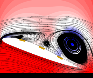
Figure 7 shows the process of vortex generated from the upper surface being influenced by flow control. The time of each flow field snapshot is also indicated in figure 6. In figure 6(a), a backflow effect is generated in front of jet 1, so the action 1 maximizes the suction to create an attachment effect on forward flow. Then the vortex in green box moves by the jet 2 in figure 6(b) and hence $t=17.3$ is the time when the suction action is strongest. When the vortex moves above the jet 3 with $t=17.9$, the injection of jet 3 will enhance the intensity of the reverse flow of fluid at the interface between the vortex and the surface. Therefore, the action of jet 3 is at its lowest point, while jet 1 and jet 2 still help the fluid to reattach. In figure 6(d), in addition to the jet affecting the generation of a new vortex, as shown in figure 6(a), jet 3 also promotes vortex shedding in the green box at maximum jet velocity. Due to the increase in flow velocity caused by the jet, the reverse pressure gradient at the tail is also strengthened, which can also be seen in the periodic-averaged surface pressure distribution in figure 6.

Figure 7. Flow field snapshot of Munk M-6 airfoil with flow control. Black represents streamline, and the background is instantaneous pressure contour. (a) Jet 1 maximizes the suction to create an attachment effect. (b) Jet 2 maximizes the suction to strengthen the attachment effect. (c) Jet 3 minimizes the injection to avoid enhancing local backflow. (d) Jet 3 maximizes the injection to promote vortex shedding, but also enhances the backflow effect at the tail end. (a) $t=16.6$, (b) $t=17.3$, (c) $t=17.9$ and (d) $t=18.5$.

Figure 8 presents a comparison between our transformer-based policy improvement operator and PPO agent, showcasing results from three repeated experiments. The solid lines represent the mean learning SoR for different experiments on the same case, while the coloured bands indicate the standard deviation. As anticipated, the policy improvement operator outperforms PPO agents with limited interactions in LIBECK L1003, NASA LRN 1015 and LANGLEY NLF 0414F. These results demonstrate that the learning mode proposed in this experiment can, to some extent, replace reinforcement learning agents when flow control strategies require repeated learning. However, enhancing the learning ability of this operator necessitates more data on various airfoils and cases, representing a crucial avenue for advancing towards more generalized fluid models in the future.

Figure 8. Evaluation performance of policy improvement operator (in red) and reinforcement learning (in blue) on airfoil flow separation. Under limited number of interactions, the policy improvement operator outperforms in three evaluation new cases. (a) Evaluation LIBECK L1003, (b) evaluation NASA LRN 1015 and (c) evaluation LANGLEY NLF 0414F.

4.2. Multi-airfoil AFC policy learning for airfoil shape optimization design

This subsection extends the application of the proposed in-context active flow control policy learning framework to the aerodynamic optimization of airfoils, a critical and well-researched area in the field. The article uses industry-standard methods, particularly surrogate-based approaches (Forrester, Sobester & Keane Reference Forrester, Sobester and Keane2008; Han & Zhang Reference Han and Zhang2012), as shown in figure 9. Using the class function/shape function transformation method (CST) (Kulfan Reference Kulfan2008), the airfoil shape is parametrized into a vector. A surrogate model is then built to estimate the aerodynamic forces for each airfoil CST vector. The global optimization algorithm uses the surrogate model's predictions to infer the optimal airfoil shape, avoiding the need for repeated CFD simulations. At each iteration, the predicted optimal airfoil is simulated with CFD, and the results are added as new sample points to update the surrogate model, continuously refining predictions for the next optimal airfoil. In this framework, the transformer-based policy improvement operator is dedicated solely to quickly learning flow control policies for the optimized airfoils, without directly contributing to the shape optimization. In figure 9(a), solid lines represent the aerodynamic optimization process, while dashed lines indicate the flow control learning. A detailed method explanation can be found in Appendix E.

Figure 9. Integration of reinforcement learning and aerodynamic shape optimization. (a) Flowchart of aerodynamic shape optimization framework. (b) Dynamic optimization process of surrogate model.

This study takes the NACA0012 airfoil as the benchmark, with a deformation range constraint of 20 $\%$, and the optimization objective is to maximize the lift drag ratio of the airfoil, as follows:

(4.1)\begin{align} \max \quad &C_l/C_d \end{align}
(4.2)\begin{align} {{\rm such\ that}} \quad &C_l/C_d > {C_l/C_d}_{benchmark} \end{align}
(4.3)\begin{align} &\max T \geq \max T_{benchmark} \end{align}
(4.4)\begin{align} &\min T \leq \min T_{benchmark}, \end{align}

where $C_l$ is the lift coefficient, $C_d$ is the drag coefficient and $T$ is the thickness. The process of dynamic sampling is illustrated in figure 9. Most of the latest sampled points, with a redder colour, will be concentrated in the lower right corner, which is the area with a high lift-to-drag ratio. After fifty iterations, the optimization process ends.

Every ten iterations, active flow control is introduced to the airfoil corresponding to the maximum $C_l/C_d$ predicted by the model to enhance aerodynamic performance. Figure 10 illustrates the performance of the active flow control rapid adaptation framework on these six new airfoils. As observed in previous results, the policy consistently improves through interactions until convergence. The capacity for in-context learning further boosts the efficiency of policy improvement by eliminating the need for training.

Figure 10. Learning progress via policy improvement operator on new airfoils generated from aerodynamic shape optimization progress.

Figure 11 compares the aerodynamic performance of the benchmark airfoil, optimized airfoil and airfoil with applied flow control for a more intuitive explanation. The $SoR$s are plotted on the vertical axis, with six optimized airfoils presented on the horizontal axis. From an aesthetic standpoint, the optimized airfoil after fifty iterations exhibits the smoothest shape, indicating an anticipated improvement in performance. Except for the first one, the aerodynamic performances of the other airfoils without flow control surpass the benchmark. In comparison with the benchmark, the optimized airfoil sees a $41.23\,\%$ increase, while the airfoil with active flow control achieves a $54.72\,\%$ improvement in terms of the $SoR$. This outcome aligns with the study's goal, demonstrating the ability to achieve active flow control policy in-context learning on various cases using only one trained network.

Figure 11. Performance enhancement from aerodynamic shape optimization and active flow control. The shape of the corresponding airfoil is drawn below the horizontal axis.

For clarity, periodic-average surface pressure distributions and pressure fields are relatively drawn in figures 12 and 13. Figure 12(a) shows the results of CST-based aerodynamic shape optimization, with beneficial improvements on both the upper and lower surfaces. In figure 12(b), active flow control mainly changes the pressure distribution on the upper surface, with lower periodic pressure in front of the upper surface. The reason for the increase in periodic pressure near the trailing edge was explained in the previous chapters. These results also match well with the results of the periodic average pressure field, as shown in figure 13.

Figure 12. Comparison between shape-optimized, controlled and uncontrolled periodic-average surface pressure distribution. The pressure near the tail of the upper surface has also increased, similar to the situation of Munk M-6. (a) Periodic-averaged surface pressure distribution of benchmark and shape-optimized airfoil and (b) periodic-averaged surface pressure distribution of shape-optimized airfoils with control and without control.

Figure 13. Comparison between controlled and uncontrolled periodic-average pressure field. The flow field results are consistent with the pressure distribution results. (a) Uncontrolled periodic-average pressure field and (b) controlled periodic-average pressure field.

5. Conclusions

In this study, we propose a novel active flow control policy learning framework via an improvement operator. Employing the proximal policy optimization algorithm, we collect extensive learning histories from various cases as sequences. The framework incorporates an agent built on a transformer architecture to conceptualize the reinforcement learning process as a causal sequence prediction problem. With a sufficiently extended context length, the agent learns not a static policy but rather a policy improvement operator. When confronted with new flow control cases, such as those involving new airfoils, the agent performs policy learning entirely in-context. This implies that there is no need to update network parameters during the learning process, showcasing the adaptability and efficiency of the proposed framework for continuous learning in scientific control problems.

This study explores two active flow control environments: vortex-induced vibration and airfoil flow separation. The results notably illustrate the adept learning capabilities of the intelligent agent across diverse cases. Moreover, the paper emphasizes the seamless integration of this learning framework with existing research methods, particularly in the context of airfoil optimization design. This integration eliminates the necessity for training new flow control cases from scratch, highlighting the importance of the proposed approach. Although flow control and shape optimization are currently conducted separately – meaning the control strategy is developed based on the shape-optimized airfoil – there must ultimately be a common objective function for enhanced performance (Pehlivanoglu & Yagiz Reference Pehlivanoglu and Yagiz2011; Zhang & He Reference Zhang and He2015). Looking ahead, it is conceivable that the entire process, from developing flow control policies to the overall system design of vehicles, could be accomplished through the cooperation of reinforcement learning for optimization (Viquerat et al. Reference Viquerat, Rabault, Kuhnle, Ghraieb, Larcher and Hachem2021) and the transformer as a universal model. It is crucial to highlight that while the demonstrated policies exhibit effectiveness, achieving further performance improvements necessitates additional training cases. Future developments in the field of artificial intelligence in fluid dynamics should consider the establishment of multi-task general models capable of handling substantial data. This direction holds promise for advancing the sophistication and applicability of learned policies in diverse fluid-related applications.

To the author's knowledge, this study is one of the first to use transformer architecture to design active flow control policies for various airfoils. Transformer networks excel at capturing long-range dependencies within input data, making them ideal for modelling the time-dependent behaviour. Their parallel processing capabilities allow for faster training times compared with architectures that process data sequentially, such as RNNs, which is particularly appealing for handling long sequences and large datasets (Vaswani et al. Reference Vaswani, Shazeer, Parmar, Uszkoreit, Jones, Gomez, Kaiser and Polosukhin2017). This study uses transformer architectures to construct a policy improvement operator from complex across-episodic training histories. However, this article did not explore the output performance of the transformer. At the same time, we also note that many previous studies have achieved success in studying the curse of action space dimensions (Belus et al. Reference Belus, Rabault, Viquerat, Che, Hachem and Reglade2019; Vignon et al. Reference Vignon, Rabault, Vasanth, Alcántara-Ávila, Mortensen and Vinuesa2023a; Peitz et al. Reference Peitz, Stenner, Chidananda, Wallscheid, Brunton and Taira2024). Leveraging invariants in the domain, there could be higher expectations for the transformer architecture's ability to handle long sequences with more complex dimension and the local agent setting to avoid the curse of dimensionality on the control space dimension.

Following Tang et al. (Reference Tang, Rabault, Kuhnle, Wang and Wang2020), this study once again uses one machine learning model to tackle various reinforcement-learning-based active flow control cases. This innovative approach offers a fresh perspective on the advancement of the reinforcement-learning-based active flow control field. The anticipation is that this work not only introduces inventive ideas to the readers but also showcases the collaborative potential of machine learning technologies, specifically reinforcement learning and transformers, in the domain of flow control. The exploration of a unified model for diverse cases opens new avenues for efficiency and adaptability in addressing complex challenges within the domain of active flow control.

Funding

The authors gratefully acknowledge the support of the National Natural Science Foundation of China (grant no. 92271107).

Declaration of interests

The authors report no conflict of interest.

Appendix A. Proximal policy optimization

The algorithms have been presented in detail previously (Kakade & Langford Reference Kakade and Langford2002; Schulman et al. Reference Schulman, Wolski, Dhariwal, Radford and Klimov2017; Queeney, Paschalidis & Cassandras Reference Queeney, Paschalidis and Cassandras2021), and a brief explanation is provided here. The objective function of reinforcement learning is defined as (2.2), or in another form, with state value function $v_{{\rm \pi} _\theta }$:

(A1)\begin{equation} J({\rm \pi} _\theta)=v_{{\rm \pi} _\theta}(s_0), \end{equation}

where $s_0$ is the initial state and $v_{{\rm \pi} _\theta }(s_0)=E_{\tau \sim {\rm \pi}, s_0}[\sum _{t=1}^{T} \gamma ^t r_t]$ is the state value function. There is also a state-action value function $q_{{\rm \pi} _\theta }(s_0, a_0)$, defined as $q_{{\rm \pi} _\theta }(s_o, a_o)=E_{\tau \sim {\rm \pi}, s_0, a_0}[\sum _{t=1}^{T} \gamma ^t r_t]$. Next, the improvement between new and old policies is calculated:

(A2)\begin{align} J({\rm \pi} _{new})-J({\rm \pi} _{old}) &= E_{\tau \sim {\rm \pi}_{new}}\left[\sum_{t=0}^T r_t\right] - E_{\tau \sim {\rm \pi}_{old}}\left[\sum_{t=0}^T r_t\right] \nonumber\\ &= E_{\tau \sim {\rm \pi}_{new}}\left[\sum_{t=0}^T r_t - v_{{\rm \pi} _{old}} (s_0)\right] \nonumber\\ &=E_{\tau \sim {\rm \pi}_{new}}\left[\sum_{t=0}^T \gamma^t(r_t + \gamma v_{{\rm \pi} _{new}}(s_{t+1}) - v_{{\rm \pi} _{old}}(s_t))\right], \end{align}

where $\tau =(s_0, a_0, r_0, s_1, a_1, r_1, s_2, \ldots )$. Let $A_{{\rm \pi} _{old}}(s_t, a_t) = r_t + \gamma v_{{\rm \pi} _{new}}(s_{t+1}) - v_{{\rm \pi} _{old}}(s_t)$, which is defined as the advantage function. Additionally, the improvement is

(A3)\begin{align} J({\rm \pi} _{new})-J({\rm \pi} _{old}) &= E_{\tau \sim {\rm \pi}_{new}}[A_{{\rm \pi} _{old}}(s_t, a_t)] \nonumber\\ &= \sum_{t=0}^T \gamma^t \sum_{s_t} Pr(s_0 \rightarrow s_t, s_t, t, {\rm \pi}_{new})\sum_{a_t}{\rm \pi} _{new}(a_t\,|\,s_t)A_{{\rm \pi} _{old}(s_t,a_t)} \nonumber\\ &= \sum_{s} \rho^{{\rm \pi} _{new}}(s) \sum_{a}{\rm \pi} _{new}(a \mid s)A_{{\rm \pi} _{old}(s,a)}. \end{align}

Here, $\rho ^{\rm \pi} (s)=\sum _{t=0}^T \gamma ^t Pr(s_0 \rightarrow s, s, t, {\rm \pi} _\theta )$ is the discounted state distribution. Obviously, $\sum _{s} Pr(s_0 \rightarrow s, s, t, {\rm \pi} _\theta) = 1$, $\sum _{a}{\rm \pi} (a \mid s)=1$. The summation of $\rho ^{\rm \pi} (s)$ is $\sum _s \rho ^{\rm \pi} (s) = \sum _{t=0}^T \gamma ^t \sum _s Pr(s_0 \rightarrow s, s, t, {\rm \pi} _\theta ) = {1}/({1-\gamma })$. Let $d^{\rm \pi} (s) = (1-\gamma )\rho ^{\rm \pi} (s)$, representing state visitation distributions, and the improvement is calculated by

(A4)\begin{align} J({\rm \pi} _{new})-J({\rm \pi} _{old}) &= \sum_{s} \rho^{{\rm \pi} _{new}}(s) \sum_{a}{\rm \pi} _{new}(a \mid s)A_{{\rm \pi} _{old}(s,a)} \nonumber\\ &= \frac{1}{1-\gamma} E_{s \sim d^{{\rm \pi} _{new}}, a \sim {{\rm \pi} _{new}}}[A_{{\rm \pi} _{old}(s,a)}] \nonumber\\ &= \frac{1}{1-\gamma} E_{s \sim d^{{\rm \pi} _{old}}, a \sim {{\rm \pi} _{new}}}[A_{{\rm \pi} _{old}(s,a)}] \nonumber\\ &\quad + \frac{1}{1-\gamma} \{ E_{s \sim d^{{\rm \pi} _{new}}, a \sim {{\rm \pi} _{new}}}[A_{{\rm \pi} _{old}(s,a)}] \nonumber\\ &\quad - E_{s \sim D^{{\rm \pi} _{old}}, a \sim {{\rm \pi} _{new}}}[A_{{\rm \pi} _{old}(s,a)}] \} \nonumber\\ &\geq \frac{1}{1-\gamma} E_{s \sim d^{{\rm \pi} _{old}}, a \sim {{\rm \pi} _{new}}}[A_{{\rm \pi} _{old}(s,a)}] \nonumber\\ &\quad - \frac{1}{1-\gamma} | E_{s \sim d^{{\rm \pi} _{new}}, a \sim {{\rm \pi} _{new}}}[A_{{\rm \pi} _{old}(s,a)}] \nonumber\\ &\quad - E_{s \sim d^{{\rm \pi} _{old}}, a \sim {{\rm \pi} _{new}}}[A_{{\rm \pi} _{old}(s,a)}] |. \end{align}

According to the Holder inequality,

(A5)\begin{align} J({\rm \pi} _{new})-J({\rm \pi} _{old}) &\geq \frac{1}{1-\gamma} E_{s \sim D^{{\rm \pi} _{old}}, a \sim {{\rm \pi} _{new}}}[A_{{\rm \pi} _{old}(s,a)}] \nonumber\\ &\quad -\frac{1}{1-\gamma}\|d^{{\rm \pi} _{new}}-d^{{\rm \pi} _{old}}\|_1 \|E_{s \sim D^{{\rm \pi} _{old}}, a \sim {{\rm \pi} _{new}}}[A_{{\rm \pi} _{old}(s,a)}]\|_\infty. \end{align}

Lemma A.1 (Achiam et al. Reference Achiam, Held, Tamar and Abbeel2017). Consider a reference policy ${\rm \pi} _{ref}$ and a future policy ${\rm \pi} $. Then, the total variation distance between the state visitation distributions $D^{{\rm \pi} _{ref}}$ and $D^{{\rm \pi} }$ is bounded by

(A6)\begin{equation} TV({\rm \pi} ,{\rm \pi} _{ref})\leq\frac{\gamma}{1-\gamma}E_{s \sim d^{{\rm \pi} _{ref}}}[TV({\rm \pi} , {\rm \pi}_{ref})(s)], \end{equation}

where $TV({\rm \pi} , {\rm \pi} _{ref})(s)$ represents the total variation distance between the distributions ${\rm \pi} ({\cdot } \mid s)$ and ${\rm \pi} _{ref}({\cdot } \mid s)$.

From the definition of total variation distance and Lemma A.1, we have

(A7)\begin{align} \|d^{{\rm \pi} _{new}}-d^{{\rm \pi} _{old}}\|_1 &= 2TV(d^{{\rm \pi} _{new}},d^{{\rm \pi} _{old}}) \nonumber\\ &\leq\frac{2\gamma}{1-\gamma}E_{s \sim d^{{\rm \pi} _{old}}}[TV({\rm \pi} _{new}, {\rm \pi}_{old})(s)] \nonumber\\ &= \frac{2\gamma}{1-\gamma}E_{s \sim d^{{\rm \pi} _{old}}}\left[\frac{1}{2}\int|{\rm \pi} _{new}(a \mid s)-{\rm \pi} _{old}(a \mid s)|\, {\rm d} a\right] \nonumber\\ &= \frac{2\gamma}{1-\gamma}E_{s \sim d^{{\rm \pi} _{old}}}\left[\frac{1}{2}\int{\rm \pi} _{old}(a \mid s)\left|\frac{{\rm \pi} _{new}(a \mid s)}{{\rm \pi} _{old}(a \mid s)}-1\right| {\rm d} a\right] \nonumber\\ &= \frac{\gamma}{1-\gamma}E_{s,a \sim d^{{\rm \pi} _{old}}}\left[\left|\frac{{\rm \pi} _{new}(a \mid s)}{{\rm \pi} _{old}(a \mid s)}-1\right|\right]. \end{align}

Also note that

(A8)\begin{equation} \|E_{s \sim D^{{\rm \pi} _{old}}, a \sim {{\rm \pi} _{new}}}[A_{{\rm \pi} _{old}(s,a)}]\|_\infty = \underset{s}{max} |E_{a\sim{{\rm \pi} ^*}}[A_{{\rm \pi} _old}(s,a)]|=C^{{\rm \pi} _{new},{\rm \pi} _{old}}. \end{equation}

Then, we can rewrite the right-hand side of (A5) as

(A9)\begin{align} J({\rm \pi} _{new})-J({\rm \pi} _{old}) &\geq \frac{1}{1-\gamma} E_{s \sim d^{{\rm \pi} _{old}}, a \sim {{\rm \pi} _{new}}}[A_{{\rm \pi} _{old}(s,a)}] \nonumber\\ &\quad - \frac{2\gamma C^{{\rm \pi} _{new},{\rm \pi} _{old}}}{(1-\gamma)^2} E_{s \sim d^{{\rm \pi} _{old}}, a \sim {{\rm \pi} _{old}}}\left[\left|\frac{{\rm \pi} _{new}(a \mid s)}{{\rm \pi} _{old}(a \mid s)}-1\right|\right] \end{align}
(A10)\begin{align} &= \frac{1}{1-\gamma}E_{s \sim d^{{\rm \pi} _{old}}, a \sim {{\rm \pi} _{old}}}\left[\frac{{\rm \pi} _{new}(a \mid s)}{{\rm \pi} _{old}(a \mid s)}A_{{\rm \pi} _{old}(s,a)}\right] \end{align}
(A11)\begin{align} &\quad - \frac{2\gamma C^{{\rm \pi} _{new},{\rm \pi} _{old}}}{(1-\gamma)^2} E_{s \sim d^{{\rm \pi} _{old}}, a \sim {{\rm \pi} _{old}}}\left[\left|\frac{{\rm \pi} _{new}(a \mid s)}{{\rm \pi} _{old}(a \mid s)}-1\right|\right]. \end{align}

The right-hand side of the inequality is called policy improvement lower bound ($PILB$), where the first term is the summary objective ($SO$) and the second term is the penalty term ($PT$). When improving, as long as the lower bound is ensured to be positive, that is, $PILB = SO - PT \geq 0$, it can ensure that the new policy is superior to the old.

To ensure $J({\rm \pi} _{new}) - J({\rm \pi} _{old}) \geq PILB \geq 0$, proximal policy optimization needs to improve $SO$, i.e

(A12)\begin{align} \underset{{\rm \pi} _{new}}{{\rm maximize}}\quad & E_{s \sim d^{{\rm \pi} _{old}}, a \sim {{\rm \pi} _{old}}}\left[\frac{{\rm \pi} _{new}(a \mid s)}{{\rm \pi} _{old}(a \mid s)}A_{{\rm \pi} _{old}(s,a)}\right] \end{align}
(A13) \begin{align} {{\rm such\ that}}\quad & E_{s \sim d^{{\rm \pi} _{old}}, a \sim {{\rm \pi} _{old}}}\left[\left|\frac{{\rm \pi} _{new}(a \mid s)}{{\rm \pi} _{old}(a \mid s)}-1\right|\right] \leq \delta. \end{align}

Here, $d^{{\rm \pi} _{old}}$ is not directly obtainable, but it can be estimated using interaction trajectories $\tau _{{\rm \pi} _{old}}$. Furthermore, incorporating constraints into the objective function

(A14)\begin{equation} L^{clip}(\theta)=E_{\tau \sim {\rm \pi}_{old}}[\min (\rho(\theta)A^{{\rm \pi} _\theta}(s,a), clip(\rho(\theta),1-\epsilon, 1+\epsilon)A^{{\rm \pi} _\theta}(s,a))], \end{equation}

where $\rho (\theta )={{\rm \pi} _\theta (a \mid s)}/{{\rm \pi} _{\theta _{old}}(a \mid s)}$ denotes the probability ratio and $\epsilon$ is the clipping parameter. Regardless of whether $A$ is greater than 0 or not, the clip mechanism can ensure that there is not much difference between the new and old policies.

Appendix B. Control cost-efficiency discussion

In our framework, the reward is indeed a combination of the lift coefficient $C_l$, drag coefficient $C_d$ and action regularization $a_t$. To provide more transparency, the reward function is structured as follows:

(B1)\begin{equation} {r_t} = \alpha {C_l}_t + \beta {C_d}_t - \gamma {\sqrt{|a_t|}}, \end{equation}

where $\alpha$, $\beta$, $\gamma$ are weightings. For flow control issues, it is important to consider energy expenditure and efficiency. In this framework, these weights, especially action regularization weightings $\gamma$, are not arbitrary but are carefully tuned to balance aerodynamic performance and cost. Our goal is to ensure that the reinforcement learning agent favours solutions that provide aerodynamic benefits while balancing energy costs associated with control actions. When we carefully selected aerodynamic targets and action regularization weights, we conducted parameter discussions on control efficiency. Here, we define a control cost-efficiency parameter, which is the increase in aerodynamic target caused by the unit active flow control mass flow rate per episode as

(B2)\begin{equation} {\eta = \frac{\overline{(\alpha {C_d} + \beta {C_l})}-\overline{(\alpha {C_d} + \beta {C_l})}_0}{\displaystyle \sum_i^n \int_{S_{jet_i}} |a_i| \cdot s \, {\rm d} s }}, \end{equation}

where the upper line represents the episodic average, $n$ is the number of the jets, subscript $0$ represents indicates the uncontrolled forces, $\alpha =1$ and $\beta =-0.5$. Then, we set up five sets of experiments to select the most suitable weighting $\gamma$ from $[0.0, 0.05, 0.1, 0.5, 1.0]$. The settings for experiment are the same as the original text, only the reward function configuration has changed. Each experiment trains a stable intelligent agent and ultimately evaluate its control cost-efficiency, as shown in figure 14.

Figure 14. Control cost-efficiency $\eta$ and force coefficients across different weightings $\gamma$. (a) Case $\gamma =0.0$ drag and lift force coefficient in one episode. (b) Case $\gamma =0.05$ drag and lift force coefficient in one episode. (c) Case $\gamma =0.1$ drag and lift force coefficient in one episode. (d) Case $\gamma =0.5$ drag and lift force coefficient in one episode. (e) Case $\gamma =1.0$ drag and lift force coefficient in one episode.

In the first configuration $\gamma =0.0$, the system achieves the maximum aerodynamic gain per unit of jet mass flow rate, as no regularization is applied to the control actions. This essentially means that the reinforcement learning agent is free to maximize aerodynamic performance without considering control costs. While the RL training converges successfully in this case, it does not result in stable physical behaviour, as indicated by the lack of periodic or steady-state forces. This instability suggests that while the agent can optimize short-term performance, it does so at the expense of physically meaningful solutions over time.

Through prior experience, we understand that control strategies involving large, unrestricted control actions often require longer simulation durations – typically more than 20 seconds per iteration – to stabilize and produce physically consistent results. Unfortunately, this was not feasible in this case, and similar instability was observed when using $\gamma =0.05$, where the action regularization was introduced but remained insufficient to promote stability over the desired simulation time frame.

Thus, we opted for the third experimental configuration with $\gamma =0.1$, which strikes a more effective balance between aerodynamic performance and control cost. With this value, the system can deliver stable results while keeping the control efforts within reasonable limits. Although some fluctuations are still present in the lift curve, as shown in panel (c), the drag curve exhibits smooth periodic behaviour, indicating that the system is physically stable overall. In addition, we consider minimizing restrictions on actions as much as possible and giving the agent a larger action space to explore reasonable control strategies in different cases.

This decision was driven by the need to ensure that the RL-based control not only optimizes aerodynamic performance but also leads to physically realistic and stable flow conditions. We believe that the combination of moderate action regularization and appropriate simulation time in the case $\gamma =0.1$ provides the best trade-off between control effectiveness and aerodynamic gains.

Appendix C. Validation on vortex-induced vibration system

Prior to conducting separation flow control experiments, this study validated the proposed active flow control framework on a vortex induced vibration system.

C.1. Numerical simulation for vortex-induced vibration

Vortex-induced vibration (VIV) (Williamson & Govardhan Reference Williamson and Govardhan2004, Reference Williamson and Govardhan2008) is a common and potentially hazardous phenomenon in flexible cylindrical structures like offshore risers and cables. As fluid flows around these structures, unsteady vortices form, leading to self-excited oscillations. This study applies active flow control to a wake oscillator model proposed by Ogink & Metrikine (Reference Ogink and Metrikine2010) to simulate VIV in cylinders, as shown in figure 15. The following dimensionless equations are used for analysis:

(C1)\begin{gather} {{\ddot x} + 2 {\varOmega}_n {\zeta} {\dot x} + {\varOmega}_n^2 x = \frac{1}{m^* + C_a} \frac{1}{2 {{\rm \pi} }^3 + {St}^2} C_{vx}}, \end{gather}
(C2)\begin{gather}{{\ddot y} + 2 {\varOmega}_n {\zeta} {\dot y} + {\varOmega}_n^2 y = \frac{1}{m^* + C_a} \frac{1}{2 {{\rm \pi} }^3 + {St}^2} C_{vy}}, \end{gather}
(C3)\begin{gather}{{\ddot q} + {\epsilon} (q^2-1) {\dot q} + q = A({\ddot x}\cos{\beta} - {\ddot y}\sin{\beta}) + Action}, \end{gather}

where $x$ is the in-flow displacement, $y$ is the cross-flow displacement, ${\varOmega }_n=6.0$ is the natural frequency, ${\zeta =0.0015}$ is the damping ratio, $m^*=5.0$ is the mass ratio, $C_a=1.0$ is the added mass coefficient, $St=0.1932$ is the Strouhal number, ${\beta =0.0}$ is the incoming angle, ${\epsilon }=0.05$ and $A=4.0$ are tuning parameters, $C_{vx}$ is the in-flow vortex force coefficient, $C_{vy}$ is the cross-flow vortex force coefficient, $q$ is the wake variable. The $Action$ parameter is added for fluidic control. The decomposed vortex forces $C_{vx}$ and $C_{vy}$ are calculated as follows:

(C4)\begin{align} C_{vx} &= \left[\hat{C}_{D0}(\cos\beta-2{{\rm \pi} }St{\dot x})-\frac{\hat{C}_{D0}q}{2}(\sin\beta-2{{\rm \pi} }St{\dot y})\right]\nonumber\\ &\quad \times {[(\cos\beta-2{{\rm \pi} }St{\dot x})^2+(\sin\beta-2{{\rm \pi} }St{\dot y})^2]^{{1}/{2}}}, \end{align}
(C5)\begin{align} C_{vy} &= [\hat{C}_{D0}(\sin\beta-2{{\rm \pi} }St{\dot y})-\frac{ \hat{C}_{D0}q}{2}(\cos\beta- 2{{\rm \pi} }St{\dot x})]\nonumber\\ & \quad \times {[(\cos\beta-2{{\rm \pi} }St{\dot x})^2+(\sin\beta-2{{\rm \pi} }St{\dot y})^2]^{{1}/{2}}}, \end{align}

where $\hat {C}_{D0}=0.1856$ is the drag force and $\hat {C}_{L0}=0.3824$ is the lift force from a stationary cylinder.

Figure 15. Decomposition of the vortex fluid force on the wake oscillator and the centroid displacement of vortex-induced vibration.

In this experiment setting, each episode spans 20 seconds, consisting of 200 interaction steps. The fourth-order Runge–Kutta method is employed to simulate the system's evolution. The controller applies a fluidic force represented by the variable $Action$ directly to the system. The control objective is to mitigate both cross-flow and in-flow vibrations. The reward function is defined as follows:

(C6)\begin{equation} {r_t} = \alpha {x_t} + \beta {{\dot x}_t}, \end{equation}

where $\alpha$ and $\beta$ are weightings. The policy improvement operator and PPO agent are trained to obtain the most rewards in one episode.

C.2. Control on vortex-induced vibration

In this experiment, we set up 36 VIV test systems with varying tuning parameters $[\epsilon, A]$ and structural system parameters $[m^*, C_a, \zeta ]$, as shown in figure 16. These parameters were randomly sampled near the upper branch values from Ogink & Metrikine (Reference Ogink and Metrikine2010). For the first 30 systems, reinforcement learning agents were trained using the PPO algorithm introduced in § 2.2. The learning curves of cases 3, 18 and 30 are shown in figure 16. Each agent interacted and learned online for 300 episodes, with the experiences stored as long sequences to train the policy improvement operator.

Figure 16. Results display of train cases on vortex-induced vibration environment. (a) Reinforcement learning progress of train cases 6, 9 and 21. (b) Parameter sets for 30 train cases (in black) and 6 evaluation cases (in red).

In the online evaluation stage, learning happens entirely in-context without updating the transformer's parameters. For evaluation cases 31–36, a context of length 2000 is pre-filled with random interactions. As seen in figure 17, the $SoR$ increases with more episodes, showing that the transformer has learned to improve policies dynamically without adjusting network parameters. We also compared the performance of the PPO algorithm in the same cases, repeating the experiment five times. The policy improvement operator outperformed the original algorithm, achieving higher rewards with the same number of episodes.

Figure 17. Evaluation performance of policy improvement operator and reinforcement learning on vortex-induced vibration. The line is the average $SoR$ among five repeated tests and the area within the standard deviation is filled with the corresponding light colour. The learning speed of policy improvement operators on new cases is generally fast and more stable.

The case involving vortex-induced vibration governed by the Ogink equation demonstrates the method's strong policy learning abilities across different structures. It also showcases effective order reduction and control in complex fluid–structure interactions, validating both the method and its parameters for future work.

Appendix D. Grid independence and time-step convergence

The validation of grid independence and time-step convergence for our computational fluid dynamics solver is detailed in tables 1 and 2. We use the NACA0012 airfoil as a benchmark, which employs the same grid generation process and time-step settings as other airfoils studied. In table 1, we examine six different grid set-ups, finding that the grid cell number increases in proportion to the number of mesh cells on the airfoil's surface. It is not until the fourth grid (G4) that the period-average lift and drag coefficients begin to show signs of convergence.

Table 1. Verification of grid independence of CFD solver (NACA0012, $Re=1000$, time step $= 0.002$, $\beta =20^{\circ }$, 20 cores, Intel(R) Xeon(R) Platinum 8175M CPU @ 2.50 GHz).

Table 2. Verification of time-step convergence of CFD solver (NACA0012, $Re=1000$, grid cell number $= 41\,903$, $\beta =20^{\circ }$, 20 cores, Intel(R) Xeon(R) Platinum 8175M CPU @ 2.50 GHz).

Additionally, six experiments are conducted to establish the independence of the time step, also presented in table 1. When the time step is reduced to less than 0.002, the variation between the period-average coefficients is less than 0.001. Given the considerations of computational efficiency, the S4 time step was selected for simulations.

As shown in figure 18, the combination of the G4 grid and S4 time step not only meets the accuracy requirements but also optimizes computational resources.

Figure 18. Comparison between different grid-sizes and time steps. (a) Grid independence. (b) Time-step convergence.

Appendix E. Surrogate-based airfoil shape optimization

This study employed a surrogate-based method to optimize the airfoil shape, significantly reducing the computational cost associated with traditional CFD-based design cycles. As demonstrated in § 4.1, optimization algorithms do not directly use the results of CFD numerical simulations, but instead use the predicted values of surrogate models. The surrogate model is constructed using Gaussian process regression (GPR) (Schulz et al. Reference Schulz, Speekenbrink and Krause2018), a powerful tool for modelling complex relationships between inputs and outputs. GPR is particularly well suited for design optimization tasks as it not only predicts the output (e.g. aerodynamic forces) but also provides a measure of uncertainty in its predictions. This allows for more informed decision-making during the optimization process. The GPR model assumes that the outputs $f(x)$ follow a Gaussian distribution $GP$, with a mean function $\mu (x)$ and a covariance function $k(x,x')$, described as

(E1)\begin{equation} {f(x)\sim GP(\mu(x), k(x,x'))}. \end{equation}

The predicted output $f(x_*)$ for a new input $x_*$ is given by the posterior mean and variance:

(E2)\begin{gather} {\mu(x_*)=k_*^TK^{{-}1}y}, \end{gather}
(E3)\begin{gather}{\delta^2(x_*)=k(x_*, x_*)-k_*^TK^{{-}1}k_*}, \end{gather}

where $k_*$ is the covariance vector between the new input $x_*$ and the training inputs $x$, $K$ is the covariance matrix of the training data, and $y$ represents the observed outputs. The covariance between points is typically modelled using a squared exponential kernel:

(E4)\begin{equation} {k(x,x')=\delta^2_f \exp\left(-\frac{\|x-x'\|^2}{2l^2}\right)}, \end{equation}

where $\delta ^2_f$ is the variance and $l$ is the length scale, controlling the smoothness of the function. The uncertainty estimates provided by GPR are crucial for guiding the optimization process, particularly in Bayesian optimization (Frazier Reference Frazier2018).

The airfoil shapes were parametrized using the class function/shape function transformation (CST) method (Kulfan Reference Kulfan2008), which simplifies complex airfoil geometries into a small set of 12 design variables. The CST method expresses the airfoil surface coordinates as a combination of class and shape functions as

(E5)\begin{equation} {z(x) = C(x) \cdot S(x)}, \end{equation}

where $x$ is the normalized chord length (ranging from 0 to 1), $C(x)$ is the class function, typically defined as

(E6)\begin{equation} {C(x) = x^{N_1}(1-x)^{N_2}}, \end{equation}

where $N_1 = 1$ and $N_2=0.5$ are control parameters, $S(x)$ is the shape function,

(E7)\begin{equation} {S(x) = \sum_{i=0}^{n} B_i^n(x) \cdot a_i}, \end{equation}

where $n=5$ is the order and $a_i$ are the coefficients that control the airfoil shape. This parametrization method reduces the complexity of the optimization problem by transforming the airfoil into a vector of design variables that can be efficiently optimized.

The optimization process itself was driven by Bayesian optimization, a sequential approach that balances exploration and exploitation using an acquisition function. One commonly used acquisition function is the expected improvement ($EI$), which is defined as

(E8)\begin{equation} {EI(x) = E[\max(0, f(x)-f(x_{best}))]}, \end{equation}

where $f(x_{best})$ is the best objective function value observed so far. The $EI$ function selects the next candidate airfoil by considering both the predicted performance and the uncertainty from the GPR model.

At each iteration shown in figure 9, the surrogate model predicts the performance of various airfoil configurations, and the acquisition function selects the next airfoil shape to be evaluated by CFD. The results from the CFD simulations are then used to update the GPR model, improving its accuracy over time. This process iterates until an optimal airfoil shape is identified, with each step efficiently guided by the Bayesian framework.

This combined approach of GPR, CST and Bayesian optimization allows for the rapid exploration of the airfoil design space while minimizing the need for costly CFD simulations. The uncertainty quantification provided by GPR enables informed decision-making, while the CST method ensures that the airfoil shapes remain both aerodynamic and practical. By employing Bayesian optimization, the study achieves a balance between exploring new design possibilities and refining known high-performing designs, leading to the identification of an optimized airfoil shape with significantly reduced computational overhead.

References

Achiam, J., Held, D., Tamar, A. & Abbeel, P. 2017 Constrained policy optimization. In International Conference on Machine Learning, pp. 22–31. PMLR.Google Scholar
Belus, V., Rabault, J., Viquerat, J., Che, Z., Hachem, E. & Reglade, U. 2019 Exploiting locality and physical invariants to design effective deep reinforcement learning control of the unstable falling liquid film. Preprint, arXiv:1910.07788.Google Scholar
Botvinick, M., Ritter, S., Wang, J.X., Kurth-Nelson, Z., Blundell, C. & Hassabis, D. 2019 Reinforcement learning, fast and slow. Trends Cogn. Sci. (Regul. Ed.) 23 (5), 408422.CrossRefGoogle ScholarPubMed
Brown, T., et al. 2020 Language models are few-shot learners. Adv. Neural Inform. Proc. Syst. 33, 18771901.Google Scholar
Cattafesta, L.N. III & Sheplak, M. 2011 Actuators for active flow control. Annu. Rev. Fluid Mech. 43, 247272.CrossRefGoogle Scholar
Chang, P.K. 2014 Separation of Flow. Elsevier.Google Scholar
Chen, L., Lu, K., Rajeswaran, A., Lee, K., Grover, A., Laskin, M., Abbeel, P., Srinivas, A. & Mordatch, I. 2021 Decision transformer: reinforcement learning via sequence modeling. Adv. Neural Inform. Proc. Syst. 34, 1508415097.Google Scholar
Choi, H., Jeon, W.-P. & Kim, J. 2008 Control of flow over a bluff body. Annu. Rev. Fluid Mech. 40, 113139.CrossRefGoogle Scholar
Choi, H., Temam, R., Moin, P. & Kim, J. 1993 Feedback control for unsteady flow and its application to the stochastic Burgers equation. J. Fluid Mech. 253, 509543.CrossRefGoogle Scholar
Collis, S.S., Joslin, R.D., Seifert, A. & Theofilis, V. 2004 Issues in active flow control: theory, control, simulation, and experiment. Prog. Aerosp. Sci. 40 (4-5), 237289.CrossRefGoogle Scholar
Deem, E.A., Cattafesta, L.N., Hemati, M.S., Zhang, H., Rowley, C. & Mittal, R. 2020 Adaptive separation control of a laminar boundary layer using online dynamic mode decomposition. J. Fluid Mech. 903, A21.CrossRefGoogle Scholar
Dong, Q., Li, L., Dai, D., Zheng, C., Wu, Z., Chang, B., Sun, X., Xu, J. & Sui, Z. 2022 A survey on in-context learning. Preprint, arXiv:2301.00234.Google Scholar
Fan, D., Yang, L., Wang, Z., Triantafyllou, M.S. & Karniadakis, G.E. 2020 Reinforcement learning for bluff body active flow control in experiments and simulations. Proc. Natl Acad. Sci. 117 (42), 2609126098.CrossRefGoogle ScholarPubMed
Forrester, A., Sobester, A. & Keane, A. 2008 Engineering Design via Surrogate Modelling: A Practical Guide. John Wiley & Sons.CrossRefGoogle Scholar
Frazier, P.I. 2018 Bayesian optimization. In Recent Advances in Optimization and Modeling of Contemporary Problems, pp. 255–278. Informs.CrossRefGoogle Scholar
Gao, C., Zhang, W., Kou, J., Liu, Y. & Ye, Z. 2017 Active control of transonic buffet flow. J. Fluid Mech. 824, 312351.CrossRefGoogle Scholar
Garnier, P., Viquerat, J., Rabault, J., Larcher, A., Kuhnle, A. & Hachem, E. 2021 A review on deep reinforcement learning for fluid mechanics. Comput. Fluids 225, 104973.CrossRefGoogle Scholar
Gazzola, M., Hejazialhosseini, B. & Koumoutsakos, P. 2014 Reinforcement learning and wavelet adapted vortex methods for simulations of self-propelled swimmers. SIAM J. Sci. Comput. 36 (3), B622B639.CrossRefGoogle Scholar
Greenblatt, D. & Wygnanski, I.J. 2000 The control of flow separation by periodic excitation. Prog. Aerosp. Sci. 36 (7), 487545.CrossRefGoogle Scholar
Guastoni, L., Rabault, J., Schlatter, P., Azizpour, H. & Vinuesa, R. 2023 Deep reinforcement learning for turbulent drag reduction in channel flows. Eur. Phys. J. E 46 (4), 27.CrossRefGoogle ScholarPubMed
Han, K., et al. 2022 A survey on vision transformer. IEEE Trans. Pattern Anal. Mach. Intell. 45 (1), 87110.CrossRefGoogle ScholarPubMed
Han, Z.-H. & Zhang, K.-S. 2012 Surrogate-based optimization. Real-World Appl. Gen. Algorithms 343, 343362.Google Scholar
Jameson, A. 2003 Aerodynamic shape optimization using the adjoint method. Lectures at the Von Kármán Institute, Brussels.Google Scholar
Janner, M., Li, Q. & Levine, S. 2021 Offline reinforcement learning as one big sequence modeling problem. Adv. Neural Inform. Proc. Syst. 34, 12731286.Google Scholar
Kakade, S. & Langford, J. 2002 Approximately optimal approximate reinforcement learning. In Proceedings of the Nineteenth International Conference on Machine Learning, pp. 267–274. Morgan Kaufmann.Google Scholar
Konishi, M., Inubushi, M. & Goto, S. 2022 Fluid mixing optimization with reinforcement learning. Sci. Rep. 12 (1), 14268.CrossRefGoogle ScholarPubMed
Kulfan, B.M. 2008 Universal parametric geometry representation method. J. Aircraft 45 (1), 142158.CrossRefGoogle Scholar
Laskin, M., et al. 2022 In-context reinforcement learning with algorithm distillation. Preprint, arXiv:2210.14215.Google Scholar
Lee, C., Kim, J. & Choi, H. 1998 Suboptimal control of turbulent channel flow for drag reduction. J. Fluid Mech. 358, 245258.CrossRefGoogle Scholar
Lee, K.-H., et al. 2022 Multi-game decision transformers. Adv. Neural Inform. Proc. Syst. 35, 2792127936.Google Scholar
Li, J., Du, X. & Martins, J.R.R.A. 2022 Machine learning in aerodynamic shape optimization. Prog. Aerosp. Sci. 134, 100849.CrossRefGoogle Scholar
Min, S., Lyu, X., Holtzman, A., Artetxe, M., Lewis, M., Hajishirzi, H. & Zettlemoyer, L. 2022 Rethinking the role of demonstrations: what makes in-context learning work? Preprint, arXiv:2202.12837.CrossRefGoogle Scholar
Ogink, R.H.M. & Metrikine, A.V. 2010 A wake oscillator with frequency dependent coupling for the modeling of vortex-induced vibration. J. Sound Vib. 329 (26), 54525473.CrossRefGoogle Scholar
Paszke, A., et al. 2019 Pytorch: an imperative style, high-performance deep learning library. Adv. Neural Inform. Proc. Syst. 32. https://proceedings.neurips.cc/paper_files/paper/2019.Google Scholar
Pehlivanoglu, Y.V. & Yagiz, B. 2011 Optimization of active/passive flow control parameters on airfoils at transonic speeds. J. Aircraft 48 (1), 212219.CrossRefGoogle Scholar
Peitz, S., Stenner, J., Chidananda, V., Wallscheid, O., Brunton, S.L. & Taira, K. 2024 Distributed control of partial differential equations using convolutional reinforcement learning. Phys. D: Nonlinear Phenom. 461, 134096.CrossRefGoogle Scholar
Queeney, J., Paschalidis, Y. & Cassandras, C.G. 2021 Generalized proximal policy optimization with sample reuse. Adv. Neural Inform. Proc. Syst. 34, 1190911919.Google Scholar
Rabault, J., Kuchta, M., Jensen, A., Réglade, U. & Cerardi, N. 2019 Artificial neural networks trained through deep reinforcement learning discover control strategies for active flow control. J. Fluid Mech. 865, 281302.CrossRefGoogle Scholar
Rabault, J., Ren, F., Zhang, W., Tang, H. & Xu, H. 2020 Deep reinforcement learning in fluid mechanics: a promising method for both active flow control and shape optimization. J. Hydrodyn. 32, 234246.CrossRefGoogle Scholar
Raymer, D. 2012 Aircraft Design: A Conceptual Approach. AIAA.CrossRefGoogle Scholar
Reddy, G., Wong-Ng, J., Celani, A., Sejnowski, T.J. & Vergassola, M. 2018 Glider soaring via reinforcement learning in the field. Nature 562 (7726), 236239.CrossRefGoogle ScholarPubMed
Reed, S., et al. 2022 A generalist agent. Preprint, arXiv:2205.06175.Google Scholar
Ren, F., Rabault, J. & Tang, H. 2021 Applying deep reinforcement learning to active flow control in weakly turbulent conditions. Phys. Fluids 33 (3), 037121.Google Scholar
Schulman, J., Levine, S., Abbeel, P., Jordan, M. & Moritz, P. 2015 Trust region policy optimization. In International Conference on Machine Learning, pp. 1889–1897. PMLR.Google Scholar
Schulman, J., Wolski, F., Dhariwal, P., Radford, A. & Klimov, O. 2017 Proximal policy optimization algorithms. Preprint, arXiv:1707.06347.Google Scholar
Schulz, E., Speekenbrink, M. & Krause, A. 2018 A tutorial on gaussian process regression: modelling, exploring, and exploiting functions. J. Math. Psychol. 85, 116.CrossRefGoogle Scholar
Shao, K., Tang, Z., Zhu, Y., Li, N. & Zhao, D. 2019 A survey of deep reinforcement learning in video games. Preprint, arXiv:1912.10944.Google Scholar
Sonoda, T., Liu, Z., Itoh, T. & Hasegawa, Y. 2023 Reinforcement learning of control strategies for reducing skin friction drag in a fully developed turbulent channel flow. J. Fluid Mech. 960, A30.CrossRefGoogle Scholar
Sutton, R.S. & Barto, A.G. 2018 Reinforcement Learning: An Introduction. MIT Press.Google Scholar
Sutton, R.S., McAllester, D., Singh, S. & Mansour, Y. 1999 Policy gradient methods for reinforcement learning with function approximation. Adv. Neural Inform. Proc. Syst. 12. https://proceedings.neurips.cc/paper_files/paper/1999.Google Scholar
Tang, H., Rabault, J., Kuhnle, A., Wang, Y. & Wang, T. 2020 Robust active flow control over a range of Reynolds numbers using an artificial neural network trained through deep reinforcement learning. Phys. Fluids 32 (5), 053605.CrossRefGoogle Scholar
Vaswani, A., Shazeer, N., Parmar, N., Uszkoreit, J., Jones, L., Gomez, A.N., Kaiser, Ł. & Polosukhin, I. 2017 Attention is all you need. Adv. Neural Inform. Proc. Syst. 30. https://proceedings.neurips.cc/paper/2017.Google Scholar
Verma, S., Novati, G. & Koumoutsakos, P. 2018 Efficient collective swimming by harnessing vortices through deep reinforcement learning. Proc. Natl Acad. Sci. 115 (23), 58495854.CrossRefGoogle ScholarPubMed
Vignon, C., Rabault, J., Vasanth, J., Alcántara-Ávila, F., Mortensen, M. & Vinuesa, R. 2023 a Effective control of two-dimensional Rayleigh–Bénard convection: invariant multi-agent reinforcement learning is all you need. Phys. Fluids 35 (6), 065146.CrossRefGoogle Scholar
Vignon, C., Rabault, J. & Vinuesa, R. 2023 b Recent advances in applying deep reinforcement learning for flow control: perspectives and future directions. Phys. Fluids 35 (3), 031301.CrossRefGoogle Scholar
Viquerat, J., Rabault, J., Kuhnle, A., Ghraieb, H., Larcher, A. & Hachem, E. 2021 Direct shape optimization through deep reinforcement learning. J. Comput. Phys. 428, 110080.CrossRefGoogle Scholar
Wang, Y.-Z., Hua, Y., Aubry, N., Chen, Z.-H., Wu, W.-T. & Cui, J. 2022 Accelerating and improving deep reinforcement learning-based active flow control: transfer training of policy network. Phys. Fluids 34 (7), 073609.Google Scholar
Wang, Z.P., Lin, R.J., Zhao, Z.Y., Chen, X., Guo, P.M., Yang, N., Wang, Z.C. & Fan, D.X. 2024 Learn to flap: foil non-parametric path palnning via deep reinforcement learning. J. Fluid Mech. 984, A9.CrossRefGoogle Scholar
Williamson, C.H.K. & Govardhan, R. 2004 Vortex-induced vibrations. Annu. Rev. Fluid Mech. 36, 413455.CrossRefGoogle Scholar
Williamson, C.H.K. & Govardhan, R. 2008 A brief review of recent results in vortex-induced vibrations. J. Wind Engng Ind. Aerodyn. 96 (6-7), 713735.CrossRefGoogle Scholar
Wolf, T., et al. 2020 Transformers: state-of-the-art natural language processing. In Proceedings of the 2020 Conference on Empirical Methods in Natural Language Processing: System Demonstrations, pp. 38–45. ACL.Google Scholar
Xie, F., Zheng, C., Ji, T., Zhang, X., Bi, R., Zhou, H. & Zheng, Y. 2023 Deep reinforcement learning: a new beacon for intelligent active flow control. Aerosp. Res. Commun. 1, 11130.CrossRefGoogle Scholar
Yan, L., Chang, X., Tian, R., Wang, N., Zhang, L. & Liu, W. 2020 A numerical simulation method for bionic fish self-propelled swimming under control based on deep reinforcement learning. Proc. Inst. Mech. Engrs C J. Mech. Engng Sci. 234 (17), 33973415.CrossRefGoogle Scholar
Yao, W. & Jaiman, R.K. 2017 Feedback control of unstable flow and vortex-induced vibration using the eigensystem realization algorithm. J. Fluid Mech. 827, 394414.CrossRefGoogle Scholar
Zhang, M. & He, L. 2015 Combining shaping and flow control for aerodynamic optimization. AIAA J. 53 (4), 888901.CrossRefGoogle Scholar
Zheng, C., Ji, T., Xie, F., Zhang, X., Zheng, H. & Zheng, Y. 2021 From active learning to deep reinforcement learning: intelligent active flow control in suppressing vortex-induced vibration. Phys. Fluids 33 (6), 063607.CrossRefGoogle Scholar
Zheng, C., Xie, F., Ji, T., Zhang, X., Lu, Y., Zhou, H. & Zheng, Y. 2022 Data-efficient deep reinforcement learning with expert demonstration for active flow control. Phys. Fluids 34 (11), 113603.CrossRefGoogle Scholar
Figure 0

Figure 1. Whole architecture of the active flow control policy learning framework via policy improvement operator.

Figure 1

Figure 2. Neural network architecture of policy improvement operator.

Figure 2

Figure 3. Configuration of airfoil flow and active flow control.

Figure 3

Figure 4. NACA-4-digit airfoil data buffer for collecting data.

Figure 4

Figure 5. Results display of train cases on airfoil flow separation environment. (a) Sum of rewards improvement between controlled flow and uncontrolled flow. (b) Learning progress via policy improvement operator on 12 new airfoils.

Figure 5

Figure 6. Episode performance of policies via policy improvement operator on Munk M-6 airfoil. (a) Three jet action trajectory. Four special annotations correspond to figure 7(ad). (b) Comparison of lift coefficient. (c) Comparison of drag coefficient. (d) Comparison of periodic-averaged surface pressure distribution. The results of controlled episode are represented in red, while those of uncontrolled episode are represented in black. The reason why the pressure near the tail of the upper surface actually increases is because the vortex is enhanced by the jet when it reaches the tail, but the overall pressure on the upper surface decreases, as explained with figure 7.

Figure 6

Figure 7. Flow field snapshot of Munk M-6 airfoil with flow control. Black represents streamline, and the background is instantaneous pressure contour. (a) Jet 1 maximizes the suction to create an attachment effect. (b) Jet 2 maximizes the suction to strengthen the attachment effect. (c) Jet 3 minimizes the injection to avoid enhancing local backflow. (d) Jet 3 maximizes the injection to promote vortex shedding, but also enhances the backflow effect at the tail end. (a) $t=16.6$, (b) $t=17.3$, (c) $t=17.9$ and (d) $t=18.5$.

Figure 7

Figure 8. Evaluation performance of policy improvement operator (in red) and reinforcement learning (in blue) on airfoil flow separation. Under limited number of interactions, the policy improvement operator outperforms in three evaluation new cases. (a) Evaluation LIBECK L1003, (b) evaluation NASA LRN 1015 and (c) evaluation LANGLEY NLF 0414F.

Figure 8

Figure 9. Integration of reinforcement learning and aerodynamic shape optimization. (a) Flowchart of aerodynamic shape optimization framework. (b) Dynamic optimization process of surrogate model.

Figure 9

Figure 10. Learning progress via policy improvement operator on new airfoils generated from aerodynamic shape optimization progress.

Figure 10

Figure 11. Performance enhancement from aerodynamic shape optimization and active flow control. The shape of the corresponding airfoil is drawn below the horizontal axis.

Figure 11

Figure 12. Comparison between shape-optimized, controlled and uncontrolled periodic-average surface pressure distribution. The pressure near the tail of the upper surface has also increased, similar to the situation of Munk M-6. (a) Periodic-averaged surface pressure distribution of benchmark and shape-optimized airfoil and (b) periodic-averaged surface pressure distribution of shape-optimized airfoils with control and without control.

Figure 12

Figure 13. Comparison between controlled and uncontrolled periodic-average pressure field. The flow field results are consistent with the pressure distribution results. (a) Uncontrolled periodic-average pressure field and (b) controlled periodic-average pressure field.

Figure 13

Figure 14. Control cost-efficiency $\eta$ and force coefficients across different weightings $\gamma$. (a) Case $\gamma =0.0$ drag and lift force coefficient in one episode. (b) Case $\gamma =0.05$ drag and lift force coefficient in one episode. (c) Case $\gamma =0.1$ drag and lift force coefficient in one episode. (d) Case $\gamma =0.5$ drag and lift force coefficient in one episode. (e) Case $\gamma =1.0$ drag and lift force coefficient in one episode.

Figure 14

Figure 15. Decomposition of the vortex fluid force on the wake oscillator and the centroid displacement of vortex-induced vibration.

Figure 15

Figure 16. Results display of train cases on vortex-induced vibration environment. (a) Reinforcement learning progress of train cases 6, 9 and 21. (b) Parameter sets for 30 train cases (in black) and 6 evaluation cases (in red).

Figure 16

Figure 17. Evaluation performance of policy improvement operator and reinforcement learning on vortex-induced vibration. The line is the average $SoR$ among five repeated tests and the area within the standard deviation is filled with the corresponding light colour. The learning speed of policy improvement operators on new cases is generally fast and more stable.

Figure 17

Table 1. Verification of grid independence of CFD solver (NACA0012, $Re=1000$, time step $= 0.002$, $\beta =20^{\circ }$, 20 cores, Intel(R) Xeon(R) Platinum 8175M CPU @ 2.50 GHz).

Figure 18

Table 2. Verification of time-step convergence of CFD solver (NACA0012, $Re=1000$, grid cell number $= 41\,903$, $\beta =20^{\circ }$, 20 cores, Intel(R) Xeon(R) Platinum 8175M CPU @ 2.50 GHz).

Figure 19

Figure 18. Comparison between different grid-sizes and time steps. (a) Grid independence. (b) Time-step convergence.