


1. Introduction
Complex fluids such as colloidal suspensions, emulsions, biological assemblies, polymer solutions and melts (Larson Reference Larson1999) are all characterised by the presence of an internal microstructure that imparts non-Newtonian flow behaviours such as yield-pseudo plasticity (Barnes Reference Barnes1999; Bonn et al. Reference Bonn, Denn, Berthier, Divoux and Manneville2017), nonlinear viscoelasticity (McKinley, Pakdel & Öztekin Reference McKinley, Pakdel and Öztekin1996; Ewoldt, Hosoi & McKinley Reference Ewoldt, Hosoi and McKinley2009), thixotropy (Mewis & Wagner Reference Mewis and Wagner2009; Larson & Wei Reference Larson and Wei2019) and thixo-elasto-visco-plasticity (Ewoldt & McKinley Reference Ewoldt and McKinley2017). These fluids arise in large-scale process equipment such as pumps, heat exchangers, mixing tanks and pipelines across industrial applications spanning minerals processing, paints and coatings, energy resources, food processing and wastewater treatment. From a process perspective, turbulent flow of these complex fluids is desirable due to improved heat and mass transfer characteristics, mitigation of sedimentation and optimal pumping efficiency. Despite widespread application, there remain significant fundamental questions regarding the turbulent flow of complex fluids.
The onset of rheological complexity in complex fluids arises from their internal microstructure, which exhibits time-dependent properties characterised by nonlinear viscoelasticity and thixotropy. Viscoelasticity involves the partial recovery of prior elastic deformation of the microstructure over small time scales (Pipkin Reference Pipkin1972), whereas thixotropy manifests as a reversible, time-dependent change in viscosity under flow conditions, driven by the shear degradation (breakdown) and the thermal recovery (rebuild) of the microstructure (Larson & Wei Reference Larson and Wei2019). Although both viscoelasticity and thixotropy involve the impact of strain rate history on the current stress state, in viscoelastic fluids, the magnitude of deformation (strain) also influences the stress response. In this sense, viscoelasticity involves the impact of both strain history and strain rate history on the current stress state, whereas thixotropy only involves the impact of strain rate history on the current stress state. Many complex fluids can be broadly classified as thixotropic elasto-visco-plastic (TEVP) materials (Ewoldt & McKinley Reference Ewoldt and McKinley2017), where the interplay of thixotropic and elastic effects, along with a plastic yield criterion, gives rise to complex rheological responses that can be difficult to deconvolve (Ewoldt & Saengow Reference Ewoldt and Saengow2022).
However, for many large-scale applications that involve continuous flow over longer time scales, some TEVP materials can be validly approximated as thixotropic fluids with shear-dependent viscosity as the elastic relaxation time scale of the fluid is several orders of magnitude shorter than both the flow and thixotropic time scales (Dullaert & Mewis Reference Dullaert and Mewis2005; Mewis & Wagner Reference Mewis and Wagner2012). One such practical example is turbulent pipe flow, where TEVP materials exhibit drag reduction primarily due to thixotropic breakdown of the microstructure near pipe walls (Escudier & Presti Reference Escudier and Presti1996; Pereira & Pinho Reference Pereira and Pinho1999, Reference Pereira and Pinho2002). Although there certainly exist industrial applications where elastic effects are important (Rosti et al. Reference Rosti, Izbassarov, Tammisola, Hormozi and Brandt2018; Izbassarov et al. Reference Izbassarov, Rosti, Brandt and Tammisola2021), many large-scale flows of complex fluids can be treated as purely thixotropic fluids (Larson & Wei Reference Larson and Wei2019) where the stress–strain relationship is purely viscous.
Despite extensive applications in the process industries (Escudier, Presti & Smith Reference Escudier, Presti and Smith1999; Pereira & Pinho Reference Pereira and Pinho1999, Reference Pereira and Pinho2002; Cayeux & Leulseged Reference Cayeux and Leulseged2020), thixotropic turbulence remains poorly understood. Turbulent thixotropic flows are complex in that they involve an interplay (Thompson Reference Thompson2020) between microstructural evolution due to thixotropy, macroscopic fluid rheology that arises from the microstructural state, and the turbulence structure that informs fluid shear and transport which drive thixotropy. The evolution of microstructure due to thixotropy is typically characterised by the structural parameter $\lambda$
(Goodeve Reference Goodeve1939; Cheng & Evans Reference Cheng and Evans1965; Barnes Reference Barnes1997) that represents the state of the microstructure, ranging from fully structured (
$\lambda$
(Goodeve Reference Goodeve1939; Cheng & Evans Reference Cheng and Evans1965; Barnes Reference Barnes1997) that represents the state of the microstructure, ranging from fully structured ( $\lambda = 1$
) to an unstructured (
$\lambda = 1$
) to an unstructured ( $\lambda = 0$
) material. Typically, the viscosity of the fluid decreases with decreasing
$\lambda = 0$
) material. Typically, the viscosity of the fluid decreases with decreasing $\lambda$
, and in a spatially homogeneous system the structural parameter decreases with shear exposure due to shear-induced structure breakdown, while simultaneously rebuilding due to Brownian motion (Nguyen & Boger Reference Nguyen and Boger1985).
$\lambda$
, and in a spatially homogeneous system the structural parameter decreases with shear exposure due to shear-induced structure breakdown, while simultaneously rebuilding due to Brownian motion (Nguyen & Boger Reference Nguyen and Boger1985).
In turbulent flows, the ubiquity of coherent structures (Lee, Kim & Moin Reference Lee, Kim and Moin1990) can generate large spatial variations in shear rate, which can generate heterogeneous spatial distributions of the structural parameter $\lambda$
. Hence, in these flows the structural parameter evolves through a balance between shear-induced microstructure breakdown, thermal rebuild and advective transport. Diffusion is typically negligible as this is governed by the very slow self-diffusion of the microstructure (Eckstein, Bailey & Shapiro Reference Eckstein, Bailey and Shapiro1977). This feedback loop remains poorly understood, particularly when the time scale of the thixotropic kinetics are similar to that of the eddy turnover time, leading to highly nonlinear flow behaviour.
$\lambda$
. Hence, in these flows the structural parameter evolves through a balance between shear-induced microstructure breakdown, thermal rebuild and advective transport. Diffusion is typically negligible as this is governed by the very slow self-diffusion of the microstructure (Eckstein, Bailey & Shapiro Reference Eckstein, Bailey and Shapiro1977). This feedback loop remains poorly understood, particularly when the time scale of the thixotropic kinetics are similar to that of the eddy turnover time, leading to highly nonlinear flow behaviour.
In this study, we explore the following questions regarding the fundamentals of thixotropic turbulence. (i) What mechanisms govern the interplay between rheology, microstructural state and turbulence structure? Understanding this relationship is essential for capturing the non-equilibrium dynamics of thixotropic turbulent pipe flows. (ii) How do these interactions evolve as the thixoviscous time scale changes? Variations in time scales can lead to qualitatively different behaviour, influencing both microstructural evolution and turbulence dynamics. (iii) Can a simplified rheological model be developed to accurately describe these interactions in fully developed turbulent flow? Development of such a model would significantly improve our ability to predict and control flow of thixotropic fluids in engineering applications.
We address these questions in this study by simulating and analysing fully developed turbulent pipe flow of a model thixotropic fluid at a moderate Reynolds number. We employ a high-resolution spectral element code (Blackburn et al. Reference Blackburn, Lee, Albrecht and Singh2019) to conduct the first direct numerical simulation (DNS) of fully developed turbulent of a thixotropic fluid. We consider a range of thixotropic kinetics relative to the eddy turnover time, as characterised by the thixoviscous number $\Lambda$
(Ewoldt & McKinley Reference Ewoldt and McKinley2017), spanning from essentially instantaneous breakdown and rebuild
$\Lambda$
(Ewoldt & McKinley Reference Ewoldt and McKinley2017), spanning from essentially instantaneous breakdown and rebuild $(\Lambda \gg 1)$
to very slow thixotropic kinetics
$(\Lambda \gg 1)$
to very slow thixotropic kinetics $(\Lambda \ll 1)$
. We analyse the Eulerian characteristics of these flows for the range of
$(\Lambda \ll 1)$
. We analyse the Eulerian characteristics of these flows for the range of $\Lambda$
and compare results with turbulent pipe flow of Newtonian and generalised Newtonian (GN) fluids. The Lagrangian frame is then used to explore the relationship between Lagrangian shear history, viscosity and flow structure across the range of
$\Lambda$
and compare results with turbulent pipe flow of Newtonian and generalised Newtonian (GN) fluids. The Lagrangian frame is then used to explore the relationship between Lagrangian shear history, viscosity and flow structure across the range of $\Lambda$
, and a stochastic model is developed for the effective viscosity, enabling elucidation of the mechanisms governing thixotropic turbulence. Despite the complex coupling between rheology, microstructure and turbulence, our findings indicate that the turbulent flow of time-dependent thixotropic fluids can be accurately captured by a time-independent (GN) effective viscosity over the entire spectrum of
$\Lambda$
, and a stochastic model is developed for the effective viscosity, enabling elucidation of the mechanisms governing thixotropic turbulence. Despite the complex coupling between rheology, microstructure and turbulence, our findings indicate that the turbulent flow of time-dependent thixotropic fluids can be accurately captured by a time-independent (GN) effective viscosity over the entire spectrum of $\Lambda$
. These effective viscosity models are verified through DNS simulations, thus providing valuable insights into the structure of thixotropic turbulence.
$\Lambda$
. These effective viscosity models are verified through DNS simulations, thus providing valuable insights into the structure of thixotropic turbulence.
The remainder of this paper is structured as follows. In § 2 the governing equations and numerical methods used are summarised. Results from the numerical simulations are analysed in the Eulerian frame in § 3, with a focus on flow behaviour and structural evolution over the range of thixotropic kinetics. A Lagrangian frame for analysis of thixotropic turbulence is developed in § 4, including derivation and validation of analytic closures for effective viscosity in the limits of fast ( $\Lambda \gg 1$
) and slow (
$\Lambda \gg 1$
) and slow ( $\Lambda \ll 1$
) thixotropic kinetics. This frame is then used in § 5 to develop and validate stochastic models for effective viscosity in the intermediate kinetics range (
$\Lambda \ll 1$
) thixotropic kinetics. This frame is then used in § 5 to develop and validate stochastic models for effective viscosity in the intermediate kinetics range ( $\Lambda \sim 1$
), and conclusions are made in § 6.
$\Lambda \sim 1$
), and conclusions are made in § 6.
2. Governing equations and numerical method
2.1. Governing equations
In this study we consider the simplest representative scenario of fully developed turbulent flow of a single-phase incompressible and inelastic thixotropic fluid through a smooth long pipe. The flow domain consists of an axially periodic straight pipe section of diameter $D$
and length
$D$
and length $L_z=4 \pi D$
with no-slip wall boundary conditions that is driven by a constant axial body force (Singh, Rudman & Blackburn Reference Singh, Rudman and Blackburn2018). Flow within the pipe is governed by the incompressible Navier–Stokes equations
$L_z=4 \pi D$
with no-slip wall boundary conditions that is driven by a constant axial body force (Singh, Rudman & Blackburn Reference Singh, Rudman and Blackburn2018). Flow within the pipe is governed by the incompressible Navier–Stokes equations
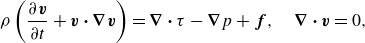 \begin{equation} \rho \left ( \frac {\partial \boldsymbol{v}}{\partial t} + \boldsymbol{v} \boldsymbol{\cdot } \boldsymbol{\nabla } \boldsymbol{v} \right ) = \boldsymbol{\nabla } \boldsymbol{\cdot } {\tau } -\boldsymbol{\nabla } p + \boldsymbol{f} ,\quad \boldsymbol{\nabla }\boldsymbol{\cdot }\boldsymbol{v} = 0, \end{equation}
where $\boldsymbol{v}$
is the fluid velocity,
$\boldsymbol{v}$
is the fluid velocity, $\rho$
is density and
$\rho$
is density and $p$
is the static pressure, and the flow is driven by the constant axial body force
$p$
is the static pressure, and the flow is driven by the constant axial body force
 \begin{equation} \boldsymbol{f} = -\frac {d\langle p\rangle }{{\rm d}z}\hat {\textbf{e}}_z. \end{equation}
The shear stress tensor ${\tau } = 2 \eta \boldsymbol{S}$
is the product of the rate of strain tensor
${\tau } = 2 \eta \boldsymbol{S}$
is the product of the rate of strain tensor $ \boldsymbol{S}=1/2 (\boldsymbol{\nabla } \boldsymbol{v} + \boldsymbol{\nabla } \boldsymbol{v}^\top )$
and the apparent viscosity
$ \boldsymbol{S}=1/2 (\boldsymbol{\nabla } \boldsymbol{v} + \boldsymbol{\nabla } \boldsymbol{v}^\top )$
and the apparent viscosity
 \begin{equation} \eta =\eta \left (\dot \gamma , \lambda \right ), \end{equation}
which is a function of local shear rate $\dot \gamma =\sqrt {2 ( \boldsymbol{S}: \boldsymbol{S})}$
and the structural parameter
$\dot \gamma =\sqrt {2 ( \boldsymbol{S}: \boldsymbol{S})}$
and the structural parameter $\lambda$
that quantifies the impact of thixotropy upon the fluid rheology. Several models for
$\lambda$
that quantifies the impact of thixotropy upon the fluid rheology. Several models for $\eta (\dot \gamma , \lambda )$
have been proposed in the literature (Moore Reference Moore1959; Toorman Reference Toorman1997; Burgos, Alexandrou & Entov Reference Burgos, Alexandrou and Entov2001; Farno, Lester & Eshtiaghi Reference Farno, Lester and Eshtiaghi2020) that cover a wide range of materials (Barnes Reference Barnes1997; Mewis & Wagner Reference Mewis and Wagner2009). Although these models are expressed in different functional forms for
$\eta (\dot \gamma , \lambda )$
have been proposed in the literature (Moore Reference Moore1959; Toorman Reference Toorman1997; Burgos, Alexandrou & Entov Reference Burgos, Alexandrou and Entov2001; Farno, Lester & Eshtiaghi Reference Farno, Lester and Eshtiaghi2020) that cover a wide range of materials (Barnes Reference Barnes1997; Mewis & Wagner Reference Mewis and Wagner2009). Although these models are expressed in different functional forms for $\eta (\dot \gamma , \lambda )$
, their behaviour is similar to a shear-thinning GN behaviours. As the fluid is inelastic, quantities such as the Deborah number and the thixoelastic number (Ewoldt & McKinley Reference Ewoldt and McKinley2017) are not relevant.
$\eta (\dot \gamma , \lambda )$
, their behaviour is similar to a shear-thinning GN behaviours. As the fluid is inelastic, quantities such as the Deborah number and the thixoelastic number (Ewoldt & McKinley Reference Ewoldt and McKinley2017) are not relevant.
For the thixotropic evolution of $\lambda$
in a homogeneous flow, various kinetic models (Barnes Reference Barnes1997; Mewis & Wagner Reference Mewis and Wagner2009; Larson Reference Larson2015) have been proposed, many of which are of the form
$\lambda$
in a homogeneous flow, various kinetic models (Barnes Reference Barnes1997; Mewis & Wagner Reference Mewis and Wagner2009; Larson Reference Larson2015) have been proposed, many of which are of the form
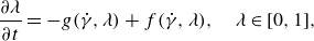 \begin{equation} \frac {\partial \lambda }{\partial t}=-g(\dot \gamma ,\lambda ) + f(\dot \gamma ,\lambda ),\quad \lambda \in [0,1], \end{equation}
where the kinetic function $g(\dot \gamma , \lambda )$
represents the shear-induced breakdown of the microstructure, while the function
$g(\dot \gamma , \lambda )$
represents the shear-induced breakdown of the microstructure, while the function $f(\dot \gamma , \lambda )$
accounts for both the thermal rebuild and the shear rebuild associated with orthokinetic coagulation (Mewis & Wagner Reference Mewis and Wagner2009). Many studies (Mujumdar, Beris & Metzner Reference Mujumdar, Beris and Metzner2002; Dullaert & Mewis Reference Dullaert and Mewis2006; Alexandrou, Constantinou & Georgiou Reference Alexandrou, Constantinou and Georgiou2009; Hewitt & Balmforth Reference Hewitt and Balmforth2013) consider similar models where the shear rate governs thixotropic degradation, however, for some materials and flow scenarios degradation is controlled by shear stress or strain energy (shear power) (Dimitriou & McKinley Reference Dimitriou and McKinley2014), resulting in different classes of thixotropic models couched in terms of, for example, shear stress as
$f(\dot \gamma , \lambda )$
accounts for both the thermal rebuild and the shear rebuild associated with orthokinetic coagulation (Mewis & Wagner Reference Mewis and Wagner2009). Many studies (Mujumdar, Beris & Metzner Reference Mujumdar, Beris and Metzner2002; Dullaert & Mewis Reference Dullaert and Mewis2006; Alexandrou, Constantinou & Georgiou Reference Alexandrou, Constantinou and Georgiou2009; Hewitt & Balmforth Reference Hewitt and Balmforth2013) consider similar models where the shear rate governs thixotropic degradation, however, for some materials and flow scenarios degradation is controlled by shear stress or strain energy (shear power) (Dimitriou & McKinley Reference Dimitriou and McKinley2014), resulting in different classes of thixotropic models couched in terms of, for example, shear stress as $g(\tau , \lambda )$
,
$g(\tau , \lambda )$
, $f(\tau , \lambda )$
(Lee & Brodkey Reference Lee and Brodkey1971; Yziquel et al. Reference Yziquel, Carreau, Moan and Tanguy1999). While these alternative thixotropic models may be more appropriate under low shear or shear yield of viscoplastic materials, the shear rate-based thixotropic models given in (2.4) may be more appropriate in high shear conditions such as turbulent flow. Consideration of thixotropic turbulence under different classes of thixotropic models is an interesting question but beyond the scope of this study.
$f(\tau , \lambda )$
(Lee & Brodkey Reference Lee and Brodkey1971; Yziquel et al. Reference Yziquel, Carreau, Moan and Tanguy1999). While these alternative thixotropic models may be more appropriate under low shear or shear yield of viscoplastic materials, the shear rate-based thixotropic models given in (2.4) may be more appropriate in high shear conditions such as turbulent flow. Consideration of thixotropic turbulence under different classes of thixotropic models is an interesting question but beyond the scope of this study.
Along with the shear viscosity $\eta$
, determination of the kinetic functions form an integral part of the rheological characterisation of thixotropic fluids. Under steady shear conditions (
$\eta$
, determination of the kinetic functions form an integral part of the rheological characterisation of thixotropic fluids. Under steady shear conditions ( $\dot \gamma =\text{const.}$
), these processes come into equilibrium and the structural parameter approaches its equilibrium value
$\dot \gamma =\text{const.}$
), these processes come into equilibrium and the structural parameter approaches its equilibrium value $\lambda \rightarrow \lambda _{\textit{eq}}(\dot \gamma )$
given by
$\lambda \rightarrow \lambda _{\textit{eq}}(\dot \gamma )$
given by
 \begin{equation} g(\dot \gamma ,\lambda _{\textit{eq}}(\dot \gamma )) = f(\dot \gamma ,\lambda _{\textit{eq}}(\dot \gamma )), \end{equation}
where typically $\lambda _{\textit{eq}}(\dot \gamma )\rightarrow 1$
as
$\lambda _{\textit{eq}}(\dot \gamma )\rightarrow 1$
as $\dot \gamma \rightarrow 0$
,
$\dot \gamma \rightarrow 0$
, $\lambda _{\textit{eq}}(\dot \gamma )\rightarrow 0$
as
$\lambda _{\textit{eq}}(\dot \gamma )\rightarrow 0$
as $\dot \gamma \rightarrow \infty$
. In general, the viscosity
$\dot \gamma \rightarrow \infty$
. In general, the viscosity $\eta (\dot \gamma ,\lambda )$
of thixotropic fluids varies strongly (typically decreasing) with both shear rate
$\eta (\dot \gamma ,\lambda )$
of thixotropic fluids varies strongly (typically decreasing) with both shear rate $\dot \gamma$
(shear thinning) and the structural parameter
$\dot \gamma$
(shear thinning) and the structural parameter $\lambda$
(thixotropy) as the microstructure responds to imposed shear.
$\lambda$
(thixotropy) as the microstructure responds to imposed shear.
As this study aims to understand the fundamental mechanisms that govern thixotropic turbulence, we consider the simplest possible non-trivial thixotropic kinetic model, where the shear breakdown $g=k\,m\,\dot \gamma \,\lambda$
and thermal rebuild
$g=k\,m\,\dot \gamma \,\lambda$
and thermal rebuild $f=m(1-\lambda )$
terms are simple linear functions of
$f=m(1-\lambda )$
terms are simple linear functions of $\dot \gamma$
and
$\dot \gamma$
and $\lambda$
, yet still capture the essential physics of more complex thixotropic models. Extension of (2.5) to heterogeneous flow such as turbulent pipe flow yields an advection–diffusion–reaction equation (ADRE) for the evolution of
$\lambda$
, yet still capture the essential physics of more complex thixotropic models. Extension of (2.5) to heterogeneous flow such as turbulent pipe flow yields an advection–diffusion–reaction equation (ADRE) for the evolution of $\lambda$
as
$\lambda$
as
 \begin{equation} \frac {\partial \lambda }{\partial t} +\boldsymbol{v} \boldsymbol{\cdot } \boldsymbol{\nabla } \lambda = m\left [-k\dot \gamma \lambda + (1- \lambda )\right ] + \alpha \boldsymbol{\nabla }^2 \lambda ,\quad 0 \leqslant \lambda \leqslant 1, \end{equation}
where $\alpha$
characterises the self-diffusivity of the microstructure which is typically very small, corresponding to Péclet number
$\alpha$
characterises the self-diffusivity of the microstructure which is typically very small, corresponding to Péclet number $Pe \sim 10^{12}$
(Morris & Brady Reference Morris and Brady1996), for example colloidal suspensions. However, a much larger value of
$Pe \sim 10^{12}$
(Morris & Brady Reference Morris and Brady1996), for example colloidal suspensions. However, a much larger value of $\alpha$
is typically used in simulations for numerical stability (Billingham & Ferguson Reference Billingham and Ferguson1993).
$\alpha$
is typically used in simulations for numerical stability (Billingham & Ferguson Reference Billingham and Ferguson1993).
The thixotropic rate parameter $m$
governs the rate of convergence of
$m$
governs the rate of convergence of $\lambda$
to the equilibrium value
$\lambda$
to the equilibrium value $\lambda _{\textit{eq}}(\dot \gamma )$
. The parameter
$\lambda _{\textit{eq}}(\dot \gamma )$
. The parameter $k$
governs the relative rates of breakdown and rebuild, and impacts the equilibrium state as
$k$
governs the relative rates of breakdown and rebuild, and impacts the equilibrium state as
 \begin{equation} \lambda _{\textit{eq}} (\dot \gamma ) = \frac {1}{1+k \dot \gamma }, \end{equation}
which also corresponds to the limit of instantaneous thixotropic kinetics $m\rightarrow \infty$
, where
$m\rightarrow \infty$
, where $\lambda \rightarrow \lambda _{\textit{eq}}(\dot \gamma )$
. Indeed, shear-thinning behaviour in non-Newtonian fluids may be conceptualised as thixotropic fluids with very rapid kinetics (Scott-Blair Reference Scott-Blair1951; Barnes Reference Barnes1997). Following the ‘eagle and rat’ metaphor (Thompson Reference Thompson2020) for homogeneous flows with time-varying shear rate, the parameter
$\lambda \rightarrow \lambda _{\textit{eq}}(\dot \gamma )$
. Indeed, shear-thinning behaviour in non-Newtonian fluids may be conceptualised as thixotropic fluids with very rapid kinetics (Scott-Blair Reference Scott-Blair1951; Barnes Reference Barnes1997). Following the ‘eagle and rat’ metaphor (Thompson Reference Thompson2020) for homogeneous flows with time-varying shear rate, the parameter $k$
defines
$k$
defines $\lambda _{\textit{eq}}(\dot \gamma )$
(position of the ‘rat’), while the parameter
$\lambda _{\textit{eq}}(\dot \gamma )$
(position of the ‘rat’), while the parameter $m$
governs the rate at which
$m$
governs the rate at which $\lambda \rightarrow \lambda _{\textit{eq}}$
, analogous to the speed at which the ‘eagle’ approaches the ‘rat’. However, for heterogeneous flows such as fully developed turbulence, this picture is more complicated as the shear rate varies spatially as well as temporally, in addition to the feedback mechanism that exists between the microstructure, rheology and turbulence. Furthermore, ADRE (2.6) can be rewritten in terms of
$\lambda \rightarrow \lambda _{\textit{eq}}$
, analogous to the speed at which the ‘eagle’ approaches the ‘rat’. However, for heterogeneous flows such as fully developed turbulence, this picture is more complicated as the shear rate varies spatially as well as temporally, in addition to the feedback mechanism that exists between the microstructure, rheology and turbulence. Furthermore, ADRE (2.6) can be rewritten in terms of $\lambda _{\textit{eq}}$
(2.7) as
$\lambda _{\textit{eq}}$
(2.7) as
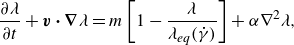 \begin{equation} \frac {\partial \lambda }{\partial t} +\boldsymbol{v} \boldsymbol{\cdot } \boldsymbol{\nabla } \lambda = m \left [1-\frac {\lambda }{\lambda _{\textit{eq}}(\dot \gamma )} \right ] + \alpha \nabla ^2\lambda , \end{equation}
that shows that the system is controlled by two competing equilibria. The first is thixotropic equilibrium, where the source term on the right-hand side of (2.8) acts to drive $\lambda$
to the stable equilibrium
$\lambda$
to the stable equilibrium $\lambda _{\textit{eq}}(\dot \gamma )$
, and the second is diffusive equilibrium, where the diffusion term on the right-hand side of (2.8) acts to drive
$\lambda _{\textit{eq}}(\dot \gamma )$
, and the second is diffusive equilibrium, where the diffusion term on the right-hand side of (2.8) acts to drive $\lambda$
to a homogeneous field. As most flows admit spatially heterogeneous shear rates, these equilibria do not coincide and so destabilise each other in a manner controlled by the relative time scales of diffusion and thixotropic evolution (given by the Damkhöler number
$\lambda$
to a homogeneous field. As most flows admit spatially heterogeneous shear rates, these equilibria do not coincide and so destabilise each other in a manner controlled by the relative time scales of diffusion and thixotropic evolution (given by the Damkhöler number $Da$
in (2.18)). In turbulent flows these equilibria are also disturbed by the inherent spatiotemporal fluctuations in the shear rate
$Da$
in (2.18)). In turbulent flows these equilibria are also disturbed by the inherent spatiotemporal fluctuations in the shear rate $\dot \gamma$
, which can dominate over these mechanisms, the relative magnitudes of which are considered in § 2.2.
$\dot \gamma$
, which can dominate over these mechanisms, the relative magnitudes of which are considered in § 2.2.
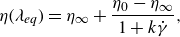
Similar to the thixotropic model, for simplicity we also consider the simplest non-trivial rheological model given a purely viscous (non-elastic) Moore fluid (Moore Reference Moore1959)
 \begin{equation} \eta (\lambda )=\eta _{\infty }+(\eta _{0}-\eta _{\infty })\lambda ,\quad \eta _{\infty } \leqslant \eta (\lambda ) \leqslant \eta _{0}, \end{equation}
where $\eta _{0}$
and
$\eta _{0}$
and $\eta _{\infty }$
represent the limiting viscosities for the structured
$\eta _{\infty }$
represent the limiting viscosities for the structured $(\lambda =1)$
and unstructured
$(\lambda =1)$
and unstructured $(\lambda =0)$
material. The coupling between the governing equations (2.1), (2.6) and (2.9) directly quantify the feedback loop between the turbulence structure, microstructural evolution and the bulk rheology.
$(\lambda =0)$
material. The coupling between the governing equations (2.1), (2.6) and (2.9) directly quantify the feedback loop between the turbulence structure, microstructural evolution and the bulk rheology.
Under equilibrium conditions, as given by (2.7), the shear-thinning GN behaviour is expected, leading to the viscosity model
 \begin{equation} \eta (\lambda _{\textit{eq}}) = \eta _\infty + \frac {\eta _0 - \eta _\infty }{1 + k\dot {\gamma }}, \end{equation}
which corresponds to a Cross model with a unit index such that deviations from the equilibrium flow curve arise due to thixotropic effects, leading to delayed viscosity changes. The model (2.10) resembles the Papanastasiou viscosity model (Papanastasiou Reference Papanastasiou1987) for yield stress fluids as it exhibits a significant viscosity reduction with only a slight increase in the stress approximated by $\eta _0/k$
(Barnes Reference Barnes2000). Under slightly different thixotropic kinetics to (2.4) which involves the shear-thinning index
$\eta _0/k$
(Barnes Reference Barnes2000). Under slightly different thixotropic kinetics to (2.4) which involves the shear-thinning index $0\lt \beta \leqslant 1$
(Barnes Reference Barnes2000), the equilibrium structural parameter
$0\lt \beta \leqslant 1$
(Barnes Reference Barnes2000), the equilibrium structural parameter $\lambda _{\textit{eq}}$
recovers the complete Cross model
$\lambda _{\textit{eq}}$
recovers the complete Cross model
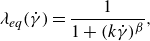 \begin{equation} \lambda _{\textit{eq}}(\dot {\gamma }) = \frac {1}{1 + (k\dot {\gamma })^\beta }, \end{equation}
and for slightly different kinetics the Carreau–Yasuda model is recovered at thixotropic equilibrium as
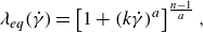 \begin{equation} \lambda _{\textit{eq}}(\dot {\gamma }) = \left [ 1 + (k\dot {\gamma })^a \right ]^{\frac {n-1}{a}}, \end{equation}
where $n$
represents that flow index and
$n$
represents that flow index and $a$
represents the Yasuda parameter that dictates the transition between Newtonian and shear-thinning regimes.
$a$
represents the Yasuda parameter that dictates the transition between Newtonian and shear-thinning regimes.
In general, there exist a broad class of shear-thinning rheological models that may be recovered as the equilibria of thixotropic models (Barnes Reference Barnes2000), and so the turbulent flow of shear-thinning and thixotropic fluids near equilibrium ( $\lambda \approx \lambda _{\textit{eq}}(\dot \gamma )$
) is expected to be qualitatively similar to that observed by, for example, Singh et al. (Reference Singh, Rudman and Blackburn2017a
,Reference Singh, Rudman and Blackburn
b
). However, significant deviations may arise for thixotropic fluids far away from equilibrium, which is the major focus of this study.
$\lambda \approx \lambda _{\textit{eq}}(\dot \gamma )$
) is expected to be qualitatively similar to that observed by, for example, Singh et al. (Reference Singh, Rudman and Blackburn2017a
,Reference Singh, Rudman and Blackburn
b
). However, significant deviations may arise for thixotropic fluids far away from equilibrium, which is the major focus of this study.
2.2. Non-dimensionalisation
The governing equations (2.1), (2.6) and (2.9) are non-dimensionalised with respect to the characteristic length scale $D$
, advective time scale
$D$
, advective time scale $\tau _v\equiv D/U_b$
and the wall viscosity
$\tau _v\equiv D/U_b$
and the wall viscosity
 \begin{equation} \eta _w = \dfrac {\tau _w}{\dot {\gamma }_w}, \end{equation}
is chosen as a viscosity scale (Rudman et al. Reference Rudman, Blackburn, Graham and Pullum2004), where subscript $w$
denotes values at the pipes walls. Henceforth all variables are non-dimensional and the same notation is used for simplicity. The resultant non-dimensional governing equations are then
$w$
denotes values at the pipes walls. Henceforth all variables are non-dimensional and the same notation is used for simplicity. The resultant non-dimensional governing equations are then
 \begin{align} &\frac {\partial \boldsymbol{v}}{\partial t} + \boldsymbol{v} \boldsymbol{\cdot } \boldsymbol{\nabla } \boldsymbol{v} = \frac {1}{Re_G} \boldsymbol{\nabla } \boldsymbol{\cdot } \left [\eta (\lambda ) \boldsymbol{\nabla } \boldsymbol{v} \right ] -\boldsymbol{\nabla } p + F\boldsymbol{f} ,\quad \boldsymbol{\nabla }\boldsymbol{\cdot }\boldsymbol{v} = 0, \end{align}
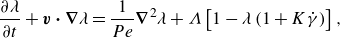 \begin{align} &\qquad \frac {\partial \lambda }{\partial t} +\boldsymbol{v} \boldsymbol{\cdot } \boldsymbol{\nabla } \lambda = \frac {1}{Pe} \boldsymbol{\nabla }^2 \lambda + \Lambda \left [1-\lambda \left (1+K\dot \gamma \right ) \right ], \end{align}
 \begin{align} &\qquad\qquad\qquad \eta (\lambda )= \eta _{\infty } \left [ 1 + \lambda (\eta _r -1) \right ]. \end{align}
In (2.14), the generalised Reynolds number
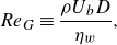 \begin{equation} Re_G\equiv \frac {\rho U_b D}{\eta _w}, \end{equation}
is used to characterise the ratio of inertial to viscous forces. As the Navier–Stokes equations do not admit dynamic similarity for non-Newtonian fluids, there exist a number of possible choices for the Reynolds number to characterise a given flow. Although $Re_G$
does not recover the laminar scaling
$Re_G$
does not recover the laminar scaling $f=64/Re_G$
(Metzner & Reed Reference Metzner and Reed1955), however, it has been shown to effectively collapse turbulent non-Newtonian datasets (Pinho & Whitelaw Reference Pinho and Whitelaw1990; Draad, Kuiken & Nieuwstadt Reference Draad, Kuiken and Nieuwstadt1998), which is more relevant for the present study. The viscosity ratio
$f=64/Re_G$
(Metzner & Reed Reference Metzner and Reed1955), however, it has been shown to effectively collapse turbulent non-Newtonian datasets (Pinho & Whitelaw Reference Pinho and Whitelaw1990; Draad, Kuiken & Nieuwstadt Reference Draad, Kuiken and Nieuwstadt1998), which is more relevant for the present study. The viscosity ratio $\eta _{r}\equiv \eta _{0}/\eta _{\infty }=2$
characterises the ratio between the fully structured and fully unstructured viscosity, and the non-dimensional body force magnitude
$\eta _{r}\equiv \eta _{0}/\eta _{\infty }=2$
characterises the ratio between the fully structured and fully unstructured viscosity, and the non-dimensional body force magnitude $F\equiv \vert d\langle {p}\rangle /{\rm d}z \vert D/ \rho U_b^2=1.8\times 10^{-2}$
characterises the ratio of inertial to body forces. This viscosity ratio is chosen primarily for simplicity and computational feasibility, allowing us to probe a wide range of thixotropic kinetics while remaining representative of real fluids such as crude oils (Chen Reference Chen1973) and pigment suspensions (Dintenfass Reference Dintenfass1962). However, much higher viscosity ratios (
$F\equiv \vert d\langle {p}\rangle /{\rm d}z \vert D/ \rho U_b^2=1.8\times 10^{-2}$
characterises the ratio of inertial to body forces. This viscosity ratio is chosen primarily for simplicity and computational feasibility, allowing us to probe a wide range of thixotropic kinetics while remaining representative of real fluids such as crude oils (Chen Reference Chen1973) and pigment suspensions (Dintenfass Reference Dintenfass1962). However, much higher viscosity ratios ( $\eta _r \sim 100$
) are common in practical fluids, such as fumed silica suspensions (Raghavan & Khan Reference Raghavan and Khan1995; Rubio-Hernández et al. Reference Rubio-Hernández, Sánchez-Toro and Páez-Flor2020) which will be explored in future studies. With respect to evolution of
$\eta _r \sim 100$
) are common in practical fluids, such as fumed silica suspensions (Raghavan & Khan Reference Raghavan and Khan1995; Rubio-Hernández et al. Reference Rubio-Hernández, Sánchez-Toro and Páez-Flor2020) which will be explored in future studies. With respect to evolution of $\lambda$
, the diffusion time scale is defined as
$\lambda$
, the diffusion time scale is defined as $\tau _{\alpha } \equiv D^2/\alpha$
and the thixotropic reaction time scale is
$\tau _{\alpha } \equiv D^2/\alpha$
and the thixotropic reaction time scale is $\tau _r \equiv 1/m$
, which characterise the Péclet and Damkhöler numbers as
$\tau _r \equiv 1/m$
, which characterise the Péclet and Damkhöler numbers as
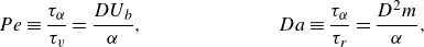 \begin{align} Pe \equiv \frac {\tau _\alpha }{\tau _v}=\frac {D U_b}{\alpha }, && Da \equiv \frac {\tau _\alpha }{\tau _r}=\frac {D^2m}{\alpha }, \end{align}
which, respectively, characterise the time scales of advection and thixotropy to the diffusive time scale. A related dimensionless parameter which characterises the time scale of thixotropic kinetics relative to that of advection (given by $\tau _v \equiv D/U_b$
) is known as the thixoviscous number (Ewoldt & McKinley Reference Ewoldt and McKinley2017)
$\tau _v \equiv D/U_b$
) is known as the thixoviscous number (Ewoldt & McKinley Reference Ewoldt and McKinley2017)
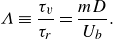 \begin{equation} \Lambda \equiv \frac {\tau _v}{\tau _r}=\frac {m D}{U_b}. \end{equation}
Here $\Lambda \gg 1$
represents thixotropic fluids that evolve on time scales much faster than the flow, whereas
$\Lambda \gg 1$
represents thixotropic fluids that evolve on time scales much faster than the flow, whereas $\Lambda \ll 1$
corresponds to thixotropic fluids that evolve over several advection times. In the absence of thixotropic kinetics (
$\Lambda \ll 1$
corresponds to thixotropic fluids that evolve over several advection times. In the absence of thixotropic kinetics ( $\Lambda = 0$
), the system becomes independent of the parameter
$\Lambda = 0$
), the system becomes independent of the parameter $K$
, such that the Moore fluid in (2.9) behaves as a Newtonian fluid with a viscosity
$K$
, such that the Moore fluid in (2.9) behaves as a Newtonian fluid with a viscosity $\eta = \eta _0$
. The non-dimensional equilibrium parameter
$\eta = \eta _0$
. The non-dimensional equilibrium parameter $K\equiv k \dot \gamma _{\text{nom}}$
in (2.15) characterises the equilibrium value of
$K\equiv k \dot \gamma _{\text{nom}}$
in (2.15) characterises the equilibrium value of $\lambda$
under the nominal shear rate
$\lambda$
under the nominal shear rate $\dot {\gamma }_{\text{nom}}$
as (2.7). This parameter although is defined as
$\dot {\gamma }_{\text{nom}}$
as (2.7). This parameter although is defined as $K\equiv k(U_b/D)$
, however, we have characterised it as
$K\equiv k(U_b/D)$
, however, we have characterised it as $K\equiv k(8U_b/D)=0.4$
to ensure that the breakdown and the rebuild occur at roughly similar rates, thus giving the largest variation of rheology with shear history. A larger
$K\equiv k(8U_b/D)=0.4$
to ensure that the breakdown and the rebuild occur at roughly similar rates, thus giving the largest variation of rheology with shear history. A larger $K$
promotes microstructural breakdown, causing the fluid rheology to approximate the fully degraded state, while a smaller
$K$
promotes microstructural breakdown, causing the fluid rheology to approximate the fully degraded state, while a smaller $K$
favours rebuild, leading the rheology towards the fully structured state. Thus, an intermediate value of
$K$
favours rebuild, leading the rheology towards the fully structured state. Thus, an intermediate value of $K$
is chosen as it maximises the interplay between turbulence, rheology and shear history, intended for the study. The generalised Reynolds number
$K$
is chosen as it maximises the interplay between turbulence, rheology and shear history, intended for the study. The generalised Reynolds number $Re_G$
is in the moderately turbulent regime, and varies by roughly a factor of
$Re_G$
is in the moderately turbulent regime, and varies by roughly a factor of $\eta _r$
due to change in viscosity with fixed
$\eta _r$
due to change in viscosity with fixed $F$
. The thixoviscous number
$F$
. The thixoviscous number $\Lambda$
is varied from slow
$\Lambda$
is varied from slow $(\Lambda \ll 1)$
to fast
$(\Lambda \ll 1)$
to fast $(\Lambda \gg 1)$
kinetics. For a finite diffusivity
$(\Lambda \gg 1)$
kinetics. For a finite diffusivity $\alpha \neq 0$
considered in numerical simulations,
$\alpha \neq 0$
considered in numerical simulations, $Pe\gg 1$
which indicates the transport of
$Pe\gg 1$
which indicates the transport of $\lambda$
is advection-dominated and that the Damkhöler number scales with
$\lambda$
is advection-dominated and that the Damkhöler number scales with $\Lambda$
as
$\Lambda$
as $Da=\Lambda \, Pe$
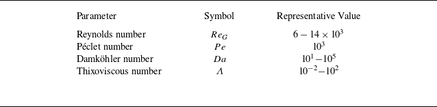
which is order unity for slow kinetics. Representative values of the key dimensionless variables used in the simulations are summarised in table 1.
$Da=\Lambda \, Pe$
which is order unity for slow kinetics. Representative values of the key dimensionless variables used in the simulations are summarised in table 1.
Table 1. Summary of key dimensionless parameters.
2.3. Numerical method
The DNS method utilised in this study is based on a GN extension nnewt (Rudman & Blackburn Reference Rudman and Blackburn2006) of the spectral element code Semtex (Blackburn et al. Reference Blackburn, Lee, Albrecht and Singh2019), which has been previously validated for the turbulent pipe flow simulations of GN fluids (Rudman & Blackburn Reference Rudman and Blackburn2006; Singh et al. Reference Singh, Rudman, Blackburn, Chryss, Pullum and Graham2016; Yousuf et al. Reference Yousuf, Kurukulasuriya, Chryss, Rudman, Rees, Usher, Farno, Lester and Eshtiaghi2024). This code is further extended to simulate turbulent flow of thixotropic fluids, as is described below. The DNS method is well suited for simulation of thixotropic turbulence as it resolves the turbulent flow across all spatiotemporal scales, eliminating the need for subgrid scale turbulent closures, and facilitating direct solution of the transport equation (2.15) for the evolution of $\lambda$
.
$\lambda$
.
The pipe cross-section is divided into discrete two-dimensional quadrilateral elements representing standard tensor-product Lagrange interpolants with Gauss–Lobatto–Legendre collocation points. The axial direction is effectively managed through the application of Fourier expansion, which naturally imposes periodic boundary conditions (Temperton Reference Temperton1992). The temporal resolution is handled by the second-order time integration method (Karniadakis, Israeli & Orszag Reference Karniadakis, Israeli and Orszag1991) to maintain numerical stability. The code strictly monitors the Courant–Friedrichs–Lewy criterion as well as the average divergence of the numerical solution for diagnostics.
To simulate thixotropy, the advective nonlinear terms in (2.14) and (2.15) are discretised explicitly, while the diffusive terms are handled implicitly to ensure numerical stability and convergence, following the methodology outlined by Rudman & Blackburn (Reference Rudman and Blackburn2006). For the breakdown and rebuild terms in (2.15), a fully implicit novel numerical scheme has been integrated into the code to enhance numerical robustness, see Appendix A for more details.
In the present study, the thixoviscous number $\Lambda$
is systematically varied in DNS computations from fast (
$\Lambda$
is systematically varied in DNS computations from fast ( $\Lambda = 10^2$
) to slow kinetics (
$\Lambda = 10^2$
) to slow kinetics ( $\Lambda = 10^{-2}$
). Simulations at higher
$\Lambda = 10^{-2}$
). Simulations at higher $\Lambda$
values were found to be infeasible, as sharp gradients in the
$\Lambda$
values were found to be infeasible, as sharp gradients in the $\lambda$
field led to numerical instabilities, even with the implicit solver detailed in Appendix A for the thixotropic kinetics. Similarly, computations for very small values of
$\lambda$
field led to numerical instabilities, even with the implicit solver detailed in Appendix A for the thixotropic kinetics. Similarly, computations for very small values of $\Lambda$
were also found infeasible, as the time scale to reach thixotropic stationarity becomes arbitrarily greater than the eddy turnover time, thus requiring extensive computational overhead. However, as shall be shown in §§ 4.2–4.3, these computational limits do not restrict understanding of thixotropic turbulence as the dynamics in the limits
$\Lambda$
were also found infeasible, as the time scale to reach thixotropic stationarity becomes arbitrarily greater than the eddy turnover time, thus requiring extensive computational overhead. However, as shall be shown in §§ 4.2–4.3, these computational limits do not restrict understanding of thixotropic turbulence as the dynamics in the limits $\Lambda \gg 1$
and
$\Lambda \gg 1$
and $\Lambda \ll 1$
can be easily understood and the behaviour at endpoints of this finite range
$\Lambda \ll 1$
can be easily understood and the behaviour at endpoints of this finite range $\Lambda \in [10^{-2},10^2]$
is close to that given by these limits. To provide reference cases, we also compute two Newtonian turbulent flow simulations corresponding to fluids with fully structured (
$\Lambda \in [10^{-2},10^2]$
is close to that given by these limits. To provide reference cases, we also compute two Newtonian turbulent flow simulations corresponding to fluids with fully structured ( $\lambda =1$
,
$\lambda =1$
, $\eta =\eta _0$
) and unstructured (
$\eta =\eta _0$
) and unstructured ( $\lambda =0$
,
$\lambda =0$
, $\eta =\eta _\infty$
) microstructures.
$\eta =\eta _\infty$
) microstructures.
The mesh design for these DNS cases adhere to the established guidelines for Newtonian (Piomelli, Liu & Liu Reference Piomelli, Liu and Liu1997) and non-Newtonian turbulence (Rudman et al. Reference Rudman, Blackburn, Graham and Pullum2004; Rudman & Blackburn Reference Rudman and Blackburn2006). The domain size $L_z = 4\pi D$
was chosen based on that used by Singh et al. (Reference Singh, Rudman and Blackburn2017a
,Reference Singh, Rudman and Blackburn
b
) which was shown to be adequate for resolving a similar flow (turbulent pipe flow of a shear thinning fluid) at
$L_z = 4\pi D$
was chosen based on that used by Singh et al. (Reference Singh, Rudman and Blackburn2017a
,Reference Singh, Rudman and Blackburn
b
) which was shown to be adequate for resolving a similar flow (turbulent pipe flow of a shear thinning fluid) at $Re \approx 12\ 000$
. The pipe cross-sectional mesh has 300 spectral elements with ninth-order tensor-product shape functions, and 384 axial data planes, corresponding to
$Re \approx 12\ 000$
. The pipe cross-sectional mesh has 300 spectral elements with ninth-order tensor-product shape functions, and 384 axial data planes, corresponding to $11.52 \times 10^6$
nodal points. Note that the structural parameter diffusivity
$11.52 \times 10^6$
nodal points. Note that the structural parameter diffusivity $\alpha$
was chosen to yield a moderate Péclet number (
$\alpha$
was chosen to yield a moderate Péclet number ( $Pe = 10^3$
) to ensure numerical stability, but this value is much smaller than characteristic values (
$Pe = 10^3$
) to ensure numerical stability, but this value is much smaller than characteristic values ( $Pe \sim 10^{12}$
) based on self-diffusivity of for example colloidal suspensions (Morris & Brady Reference Morris and Brady1996). A summary of the computational parameters is given in table 2. The DNS code monitors the Courant–Friedrichs–Lewy criterion which was kept at
$Pe \sim 10^{12}$
) based on self-diffusivity of for example colloidal suspensions (Morris & Brady Reference Morris and Brady1996). A summary of the computational parameters is given in table 2. The DNS code monitors the Courant–Friedrichs–Lewy criterion which was kept at $\ 10^{-1}$
to maintain numerical stability and convergence. Each case was run on the Gadi resource on the National Computational Infrastructure (NCI), Australia, which is a HPC cluster comprised of 8 × 24-core Intel Xeon Platinum 8274 (Cascade Lake) with 3.2 GHz CPUs and 192 GB RAM per node.
$\ 10^{-1}$
to maintain numerical stability and convergence. Each case was run on the Gadi resource on the National Computational Infrastructure (NCI), Australia, which is a HPC cluster comprised of 8 × 24-core Intel Xeon Platinum 8274 (Cascade Lake) with 3.2 GHz CPUs and 192 GB RAM per node.
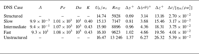
Table 2. Summary of computational parameters.
The DNS computations for the thixotropic and the structured ( $\lambda =1$
) Newtonian cases were initialised by introducing isotropic Gaussian-distributed white noise (with variance 0.01) to the velocity field of a fully developed laminar pipe flow, and the
$\lambda =1$
) Newtonian cases were initialised by introducing isotropic Gaussian-distributed white noise (with variance 0.01) to the velocity field of a fully developed laminar pipe flow, and the $\lambda$
field is set to unity. For the unstructured (
$\lambda$
field is set to unity. For the unstructured ( $\lambda =0$
) Newtonian case, the
$\lambda =0$
) Newtonian case, the $\lambda$
field is set to zero during initialisation. Under fully developed conditions the thixotropic turbulent pipe flow is symmetric and thus stationary in time, axial, and azimuthal directions but non-stationary in the radial coordinate. Each DNS computation was run until the velocity and
$\lambda$
field is set to zero during initialisation. Under fully developed conditions the thixotropic turbulent pipe flow is symmetric and thus stationary in time, axial, and azimuthal directions but non-stationary in the radial coordinate. Each DNS computation was run until the velocity and $\lambda$
fields both achieved statistical stationarity (typically 30 wash-through times), after which Eulerian turbulent flow statistics were accumulated and analysed for another 30 wash-through times. In addition, Lagrangian data (velocity, velocity gradient and
$\lambda$
fields both achieved statistical stationarity (typically 30 wash-through times), after which Eulerian turbulent flow statistics were accumulated and analysed for another 30 wash-through times. In addition, Lagrangian data (velocity, velocity gradient and $\lambda$
) were also collected for each run for
$\lambda$
) were also collected for each run for $10^4$
randomly placed tracer particles over a period of around eight wash-through times.
$10^4$
randomly placed tracer particles over a period of around eight wash-through times.
3. Eulerian characteristics of thixotropic turbulence
3.1. Instantaneous flow
In this section we examine the characteristics of fully developed thixotropic turbulent pipe flow from an Eulerian perspective. Figures 1–8 present the DNS results, while also including comparisons with the analytic closures (4.10) and (4.17) discussed in § 4. This arrangement ensures a logical flow while avoiding repetition of figures.
Figure 1 shows representative cross-sectional plots of axial velocity ( $u_z$
) fields for the two Newtonian and three thixotropic cases. The contours indicate that the Newtonian case at
$u_z$
) fields for the two Newtonian and three thixotropic cases. The contours indicate that the Newtonian case at $\lambda =0$
exhibits fine-scale structures due to high Reynolds number (table 2), while the basic velocity structure remains similar across the three thixotropic kinetics, as there is no significant change in the Reynolds number values (table 2).
$\lambda =0$
exhibits fine-scale structures due to high Reynolds number (table 2), while the basic velocity structure remains similar across the three thixotropic kinetics, as there is no significant change in the Reynolds number values (table 2).
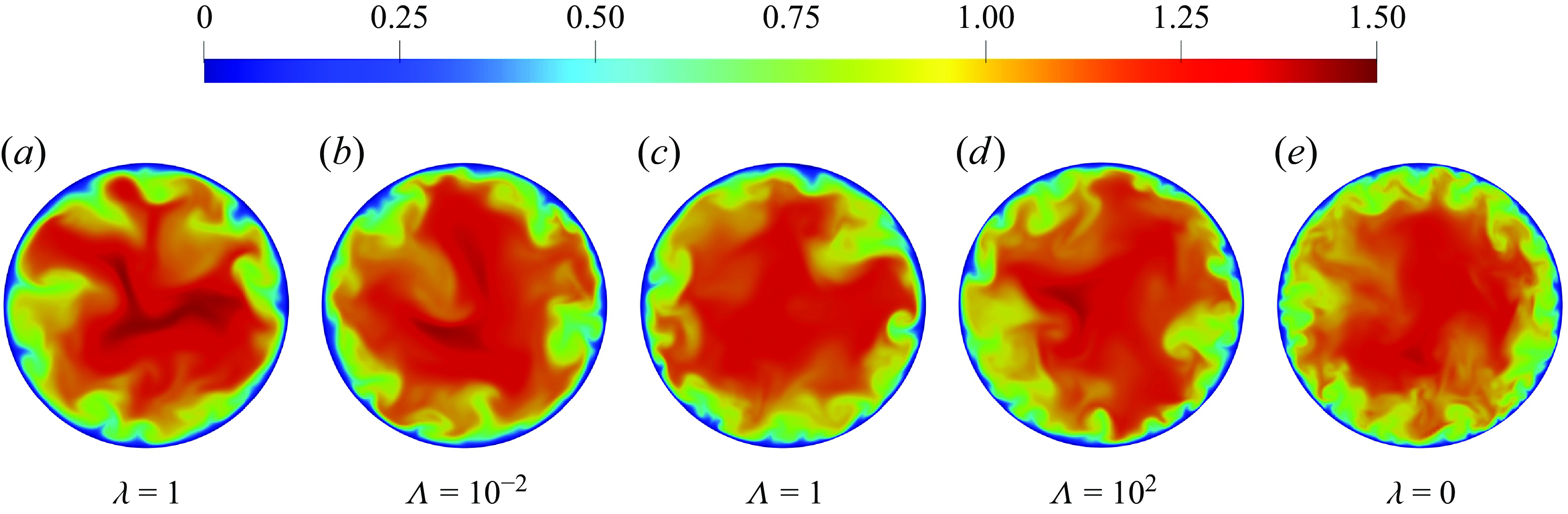
Figure 1. Typical cross-sectional contour plots of the instantaneous axial velocity $u_z(\textbf{x},t)$
for (a) Newtonian flow with
$u_z(\textbf{x},t)$
for (a) Newtonian flow with $\lambda =1$
, (b) thixotropic flow with
$\lambda =1$
, (b) thixotropic flow with $\Lambda =10^{-2}$
, (c) thixotropic flow with
$\Lambda =10^{-2}$
, (c) thixotropic flow with $\Lambda =1$
, (d) thixotropic flow with
$\Lambda =1$
, (d) thixotropic flow with $\Lambda =10^{2}$
, (e) Newtonian flow with
$\Lambda =10^{2}$
, (e) Newtonian flow with $\lambda =0$
.
$\lambda =0$
.
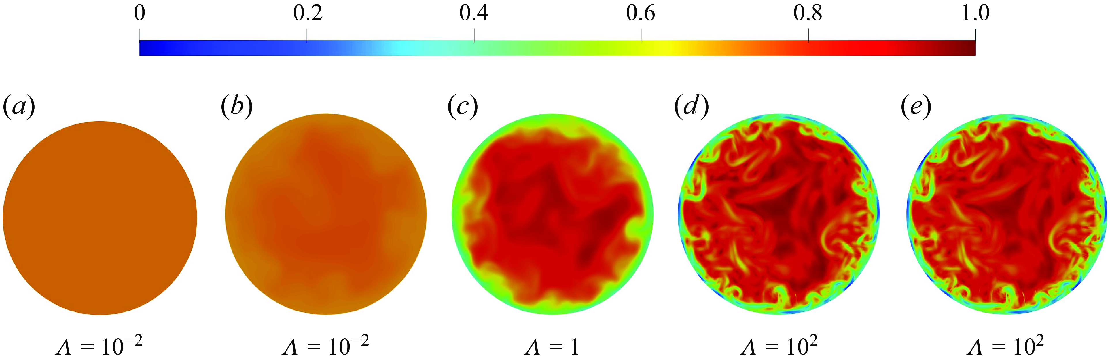
Figure 2. Typical cross-sectional contour plots of structural parameter $\lambda (\textbf{x},t)$
for (a) closure (4.17) computed from thixotropic flow with
$\lambda (\textbf{x},t)$
for (a) closure (4.17) computed from thixotropic flow with $\Lambda =10^{-2}$
, (b) thixotropic flow with
$\Lambda =10^{-2}$
, (b) thixotropic flow with $\Lambda =10^{-2}$
, (c) thixotropic flow with
$\Lambda =10^{-2}$
, (c) thixotropic flow with $\Lambda =1$
, (d) thixotropic flow with
$\Lambda =1$
, (d) thixotropic flow with $\Lambda =10^{2}$
, (e) closure (4.10) computed from thixotropic flow with
$\Lambda =10^{2}$
, (e) closure (4.10) computed from thixotropic flow with $\Lambda =10^{2}$
.
$\Lambda =10^{2}$
.
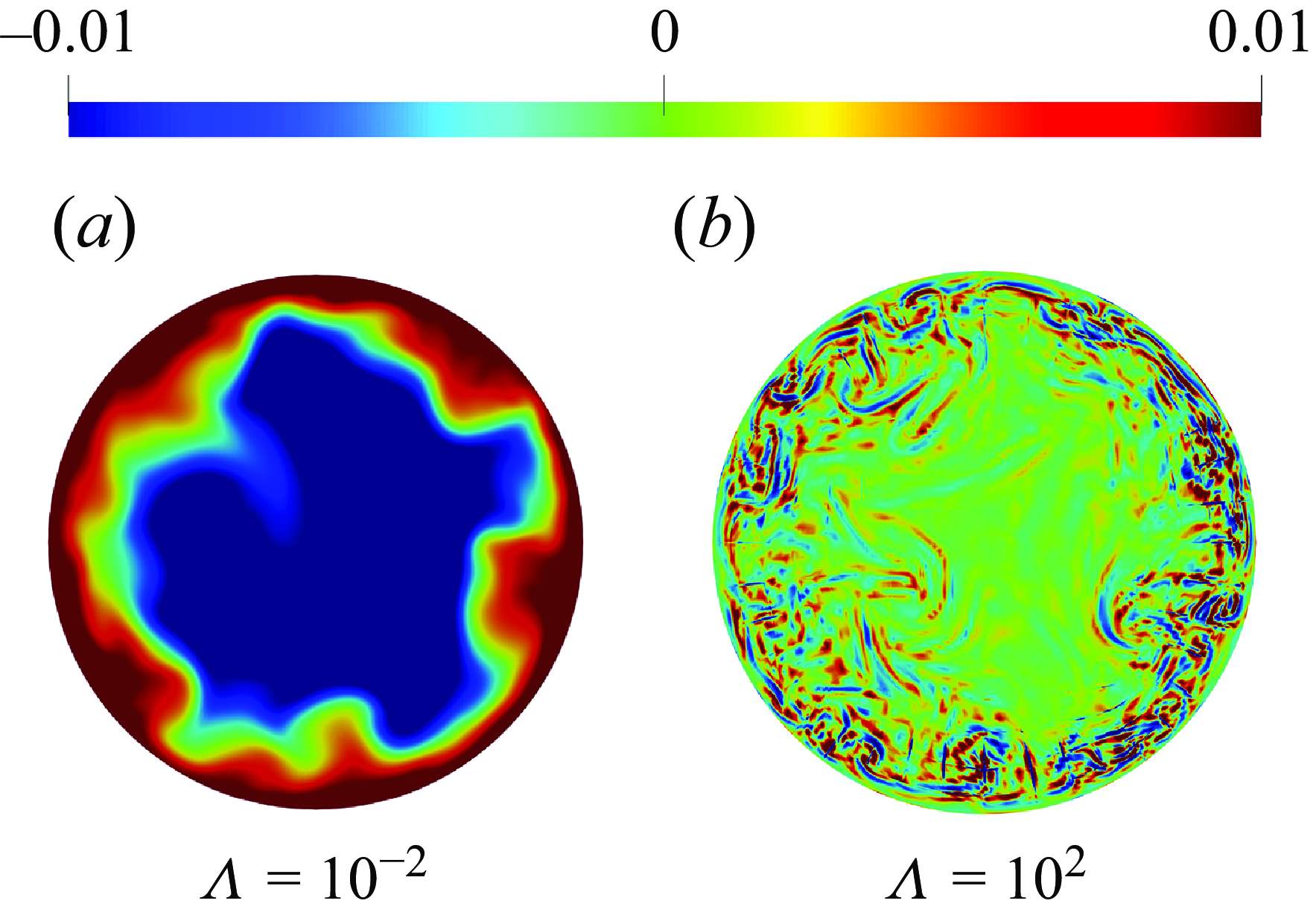
Figure 3. Deviation of typical cross-sectional contour plots of structural parameter $\Delta \lambda (\textbf{x},t)=\lambda _{\textit{lim}}(\textbf{x},t)-\lambda (\textbf{x},t)$
for (a) thixotropic flow with
$\Delta \lambda (\textbf{x},t)=\lambda _{\textit{lim}}(\textbf{x},t)-\lambda (\textbf{x},t)$
for (a) thixotropic flow with $\Lambda =10^{-2}$
against the closure (4.17) computed from thixotropic flow with
$\Lambda =10^{-2}$
against the closure (4.17) computed from thixotropic flow with $\Lambda =10^{-2}$
, (b) thixotropic flow with
$\Lambda =10^{-2}$
, (b) thixotropic flow with $\Lambda =10^{2}$
against the closure (4.10) computed from thixotropic flow with
$\Lambda =10^{2}$
against the closure (4.10) computed from thixotropic flow with $\Lambda =10^{2}$
.
$\Lambda =10^{2}$
.
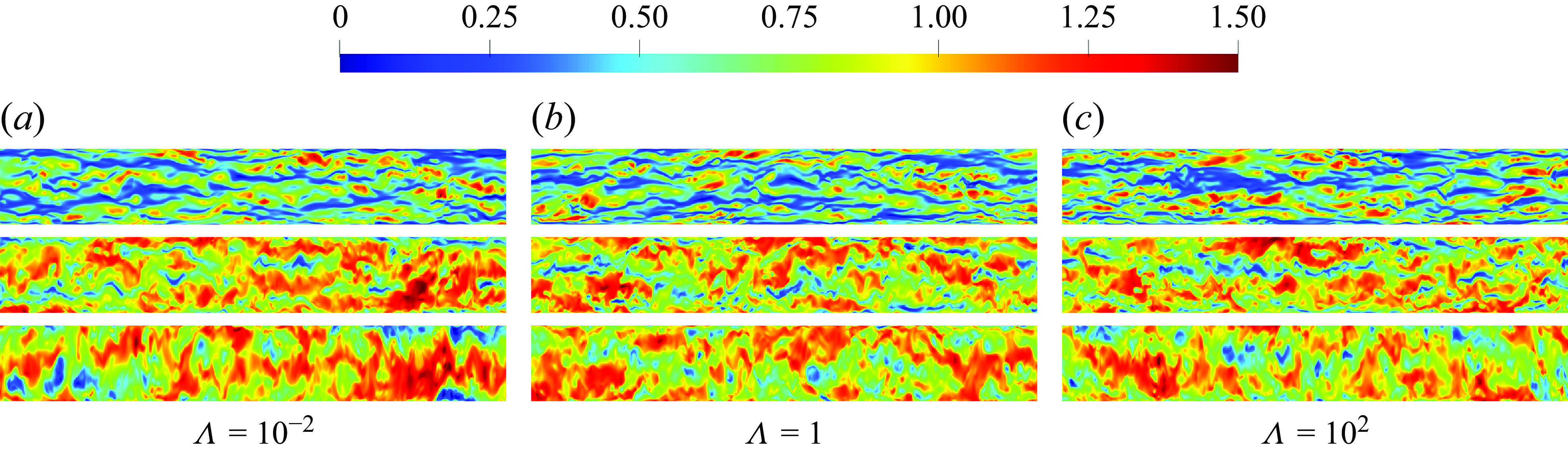
Figure 4. Typical axial contour plots of the instantaneous axial velocity $u_z(\textbf{x},t)$
at constant surfaces of
$u_z(\textbf{x},t)$
at constant surfaces of $y^+\approx$
10, 45 and 100 (from top to bottom) for thixotropic flow with (a)
$y^+\approx$
10, 45 and 100 (from top to bottom) for thixotropic flow with (a) $\Lambda =10^{-2}$
, (b)
$\Lambda =10^{-2}$
, (b) $\Lambda =1$
, (c)
$\Lambda =1$
, (c) $\Lambda =10^{2}$
. The contours have been azimuthally stretched to preserve the vertical scale.
$\Lambda =10^{2}$
. The contours have been azimuthally stretched to preserve the vertical scale.
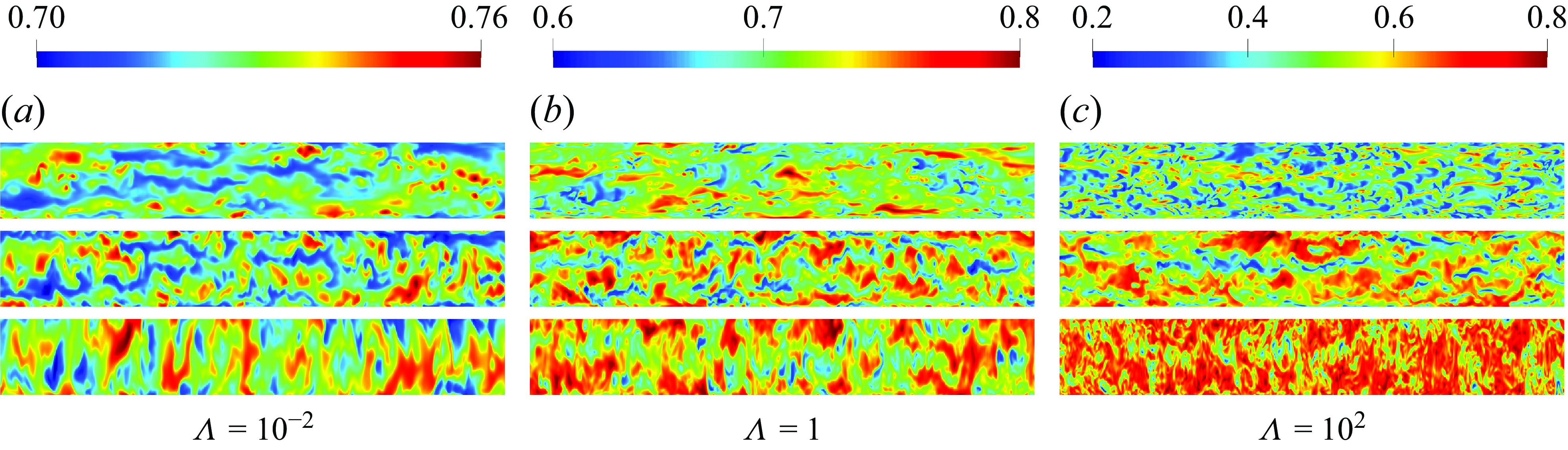
Figure 5. Typical axial contour plots of the instantaneous structural parameter $\lambda (\textbf{x},t)$
at constant surfaces of
$\lambda (\textbf{x},t)$
at constant surfaces of $y^+\approx$
10, 45 and 100 (from top to bottom) for thixotropic flow with (a)
$y^+\approx$
10, 45 and 100 (from top to bottom) for thixotropic flow with (a) $\Lambda =10^{-2}$
, (b)
$\Lambda =10^{-2}$
, (b) $\Lambda =1$
, (c)
$\Lambda =1$
, (c) $\Lambda =10^{2}$
. The contours have been azimuthally stretched to preserve the vertical scale.
$\Lambda =10^{2}$
. The contours have been azimuthally stretched to preserve the vertical scale.
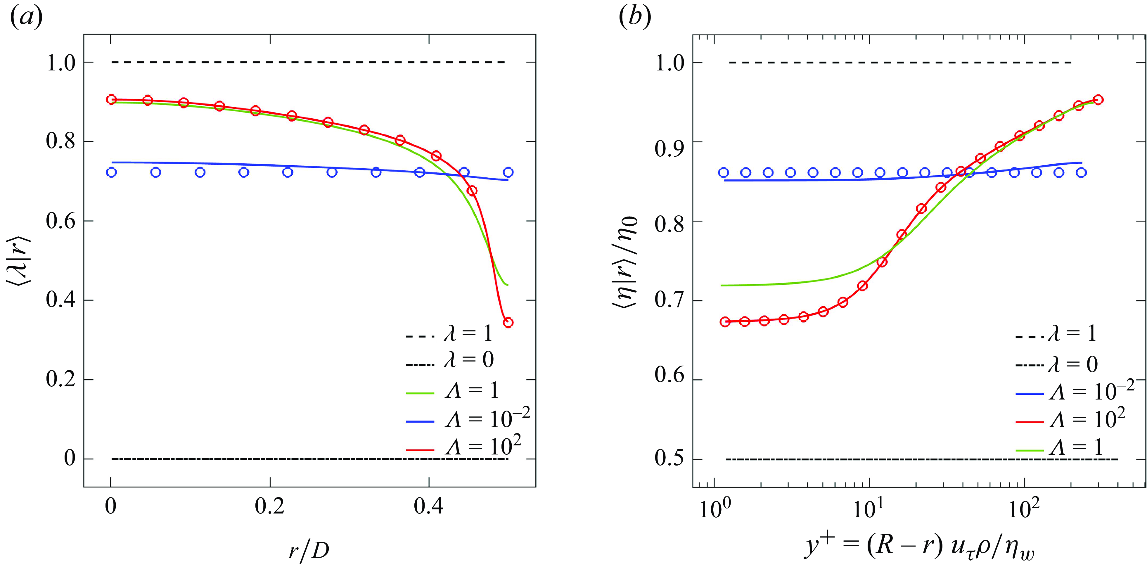
Figure 6. Radial profiles of (a) conditionally averaged structural parameter $\langle \lambda |r\rangle$
and (b) viscosity
$\langle \lambda |r\rangle$
and (b) viscosity $\langle \eta |r\rangle$
, for thixotropic flows and Newtonian reference cases. Lines indicates results from DNS computations of thixotropic and Newtonian models and circles (
$\langle \eta |r\rangle$
, for thixotropic flows and Newtonian reference cases. Lines indicates results from DNS computations of thixotropic and Newtonian models and circles ( $\boldsymbol{\circ }$
) indicate results from the analytic closures (4.17) and (4.10).
$\boldsymbol{\circ }$
) indicate results from the analytic closures (4.17) and (4.10).
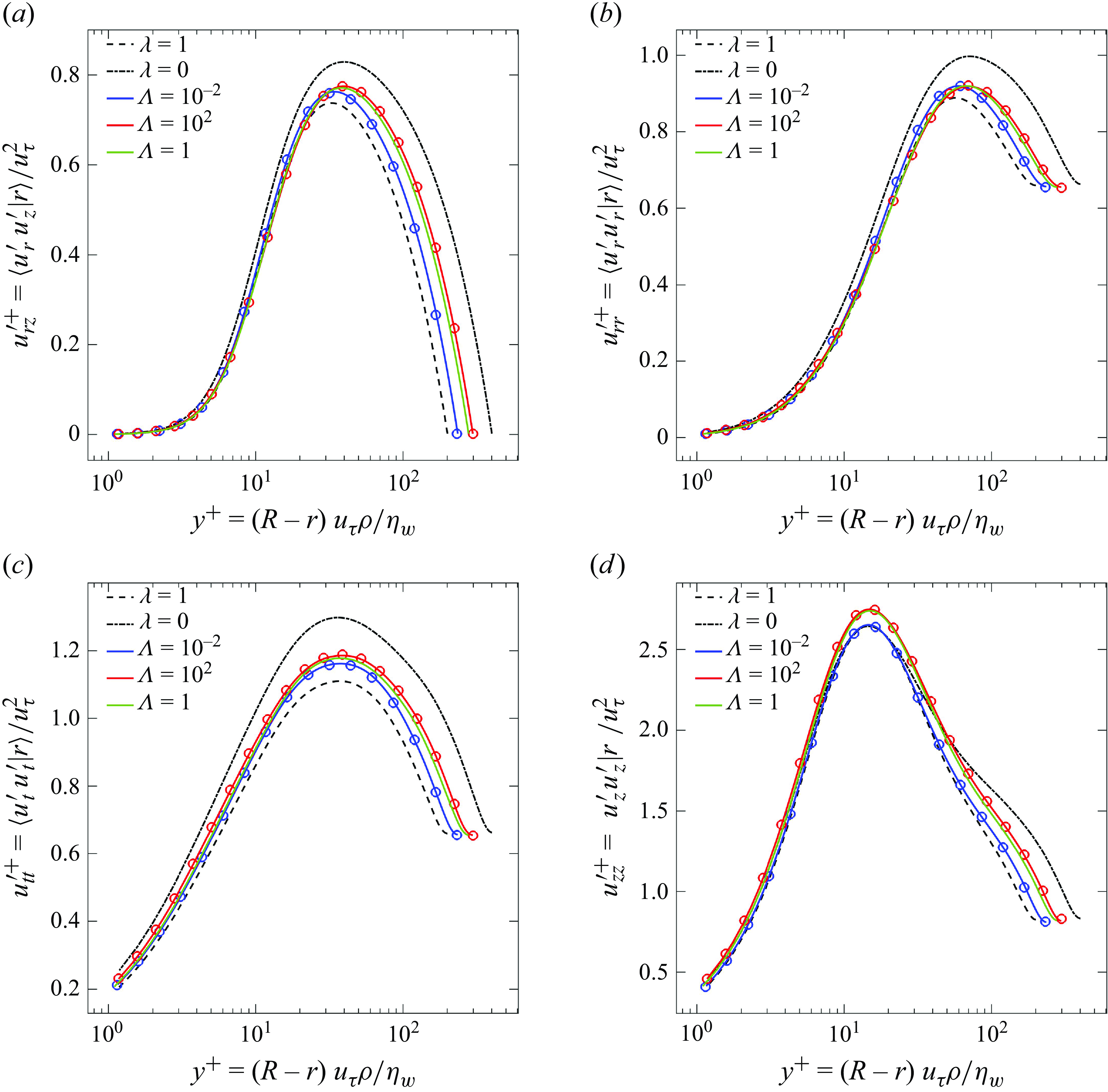
Figure 7. Radial profiles of (a) radial/axial $u'_{rz}$
, (b) radial
$u'_{rz}$
, (b) radial $u'_{rr}$
, (c) azimuthal
$u'_{rr}$
, (c) azimuthal $u'_{tt}$
and (d) axial
$u'_{tt}$
and (d) axial $u'_{zz}$
Reynolds stresses, for thixotropic flows and Newtonian reference cases. Lines indicates results from DNS computations of thixotropic and Newtonian models and circles (
$u'_{zz}$
Reynolds stresses, for thixotropic flows and Newtonian reference cases. Lines indicates results from DNS computations of thixotropic and Newtonian models and circles ( $\boldsymbol{\circ }$
) indicate results from the analytic closures (4.17) and (4.10).
$\boldsymbol{\circ }$
) indicate results from the analytic closures (4.17) and (4.10).


Figure 2 presents the corresponding structural parameter ( $\lambda$
) fields for these cases, where the contours for the Newtonian cases are excluded as they exhibit spatially uniform fields of
$\lambda$
) fields for these cases, where the contours for the Newtonian cases are excluded as they exhibit spatially uniform fields of $\lambda =1$
and
$\lambda =1$
and $\lambda =0$
. The contours show that the lambda structures are different across the three thixotropic kinetics. At larger values of
$\lambda =0$
. The contours show that the lambda structures are different across the three thixotropic kinetics. At larger values of $\Lambda$
, sharper and more fine-scale structures in the
$\Lambda$
, sharper and more fine-scale structures in the $\lambda$
field (and thus viscosity) are observed due to strong coupling between
$\lambda$
field (and thus viscosity) are observed due to strong coupling between $\lambda$
and the instantaneous shear field, and from (2.7), in the limit
$\lambda$
and the instantaneous shear field, and from (2.7), in the limit $\Lambda \gg 1$
the structural parameter is solely dependent upon the local shear rate
$\Lambda \gg 1$
the structural parameter is solely dependent upon the local shear rate $\dot \gamma$
, as demonstrated in figure 2(e). In this fast kinetics regime, the flow behaviour effectively reduces to that of a shear-thinning rheology and the turbulence structure exhibits characteristics similar to that of shear-thinning turbulence (Rudman et al. Reference Rudman, Blackburn, Graham and Pullum2004; Singh et al. Reference Singh, Rudman and Blackburn2017a
,Reference Singh, Rudman and Blackburn
b
).
$\dot \gamma$
, as demonstrated in figure 2(e). In this fast kinetics regime, the flow behaviour effectively reduces to that of a shear-thinning rheology and the turbulence structure exhibits characteristics similar to that of shear-thinning turbulence (Rudman et al. Reference Rudman, Blackburn, Graham and Pullum2004; Singh et al. Reference Singh, Rudman and Blackburn2017a
,Reference Singh, Rudman and Blackburn
b
).
For smaller values of $\Lambda$
, the structural parameter evolves more slowly along pathlines and the relevant shear rate history that governs
$\Lambda$
, the structural parameter evolves more slowly along pathlines and the relevant shear rate history that governs $\lambda$
is longer. This leads to a reduction in fine-scale structures observed in the
$\lambda$
is longer. This leads to a reduction in fine-scale structures observed in the $\lambda$
field due to an effective averaging process backwards along pathlines. Although this results in more diffuse
$\lambda$
field due to an effective averaging process backwards along pathlines. Although this results in more diffuse $\lambda$
distributions, this behaviour persists in the limit of vanishing diffusivity (
$\lambda$
distributions, this behaviour persists in the limit of vanishing diffusivity ( $Pe\rightarrow \infty )$
due to the averaging process. For these computations, diffusion of
$Pe\rightarrow \infty )$
due to the averaging process. For these computations, diffusion of $\lambda$
plays a minor role due to the moderate Péclet number (
$\lambda$
plays a minor role due to the moderate Péclet number ( $Pe=10^3$
) required for numerical stability. As the Damkhöler number scales with
$Pe=10^3$
) required for numerical stability. As the Damkhöler number scales with $\Lambda$
as
$\Lambda$
as $Da=\Lambda Pe$
, and
$Da=\Lambda Pe$
, and $Da = 10$
for
$Da = 10$
for $\Lambda = 10^{-2}$
, diffusion acts on a similar time scale as the thixotropic kinetics in this case, leading to the discrepancies later discussed in § 4.1. Note that for complex fluids
$\Lambda = 10^{-2}$
, diffusion acts on a similar time scale as the thixotropic kinetics in this case, leading to the discrepancies later discussed in § 4.1. Note that for complex fluids $Pe\gg 10^{3}$
, and so for these flows smoothing of the
$Pe\gg 10^{3}$
, and so for these flows smoothing of the $\lambda$
field is solely due to averaging of the Lagrangian shear rate. In the limit of
$\lambda$
field is solely due to averaging of the Lagrangian shear rate. In the limit of $\Lambda \ll 1$
, the
$\Lambda \ll 1$
, the $\lambda$
field is almost uniform, as demonstrated in figure 2, meaning that the viscosity is likewise and so the flow resembles that of Newtonian turbulence (Toonder & Nieuwstadt Reference den Toonder and Nieuwstadt1997; Khoury et al. Reference Khoury, Schlatter, Noorani, Fischer, Brethouwer and Johansson2013).
$\lambda$
field is almost uniform, as demonstrated in figure 2, meaning that the viscosity is likewise and so the flow resembles that of Newtonian turbulence (Toonder & Nieuwstadt Reference den Toonder and Nieuwstadt1997; Khoury et al. Reference Khoury, Schlatter, Noorani, Fischer, Brethouwer and Johansson2013).
Figure 2 also compares the thixotropic cases with closures for fast (4.10) and slow (4.17) kinetics that are developed later in § 4. These closures are quite accurate, as highlighted by the difference plots shown in figure 3 and discussed further in § 4.
Representative contour plots of axial velocity ( $u_z$
) and structural parameter (
$u_z$
) and structural parameter ( $\lambda$
) fields in the axial direction for different values of
$\lambda$
) fields in the axial direction for different values of $y^+$
for the two Newtonian and three thixotropic cases are shown in figures 4 and 5 Consistent with the contours shown in figure 1, the flow structures in figure 4 are similar across all thixotropic at different values of
$y^+$
for the two Newtonian and three thixotropic cases are shown in figures 4 and 5 Consistent with the contours shown in figure 1, the flow structures in figure 4 are similar across all thixotropic at different values of $y^+$
. These flow structures are also similar to those considered by Singh et al. (Reference Singh, Rudman and Blackburn2017b
), reinforcing the notion that turbulent thixotropic flows are qualitatively similar to shear thinning turbulent flows in general.
$y^+$
. These flow structures are also similar to those considered by Singh et al. (Reference Singh, Rudman and Blackburn2017b
), reinforcing the notion that turbulent thixotropic flows are qualitatively similar to shear thinning turbulent flows in general.
The $\lambda$
fields shown in figure 5 indicate that, as expected, the magnitude of
$\lambda$
fields shown in figure 5 indicate that, as expected, the magnitude of $\lambda$
fluctuations increases with both
$\lambda$
fluctuations increases with both $\Lambda$
and decreases with
$\Lambda$
and decreases with $y^+$
as the shear rate fluctuations are greatest near the pipe wall. In addition, the length scale of the
$y^+$
as the shear rate fluctuations are greatest near the pipe wall. In addition, the length scale of the $\lambda$
fluctuations for all
$\lambda$
fluctuations for all $y^+$
decreases with
$y^+$
decreases with $\Lambda$
as the local
$\Lambda$
as the local $\lambda$
becomes more responsive to local shear rate fluctuations with increasing thixotropic kinetics.
$\lambda$
becomes more responsive to local shear rate fluctuations with increasing thixotropic kinetics.
3.2. Turbulence statistics
Mean field and second-order statistics also provide insights into the impact of thixotropy on turbulent pipe flow. The mean radial viscosity and $\lambda$
profiles for the three thixotropic cases are illustrated in figure 6, and the Newtonian reference cases provide upper and lower bounds for these quantities.
$\lambda$
profiles for the three thixotropic cases are illustrated in figure 6, and the Newtonian reference cases provide upper and lower bounds for these quantities.
For all thixotropic cases, shear degradation in the viscous sublayer ( $y^+ \leqslant 5$
) is more significant than in the pipe core due to increased shear near the pipe walls. This is more pronounced for the faster thixotropic kinetics, as the structural parameter
$y^+ \leqslant 5$
) is more significant than in the pipe core due to increased shear near the pipe walls. This is more pronounced for the faster thixotropic kinetics, as the structural parameter $\lambda$
exhibits a stronger correlation with local shear rate
$\lambda$
exhibits a stronger correlation with local shear rate $\dot {\gamma }$
, leading to a monotone decreasing radial viscosity profile similar to that of turbulent pipe flow of shear thinning fluids (Rudman et al. Reference Rudman, Blackburn, Graham and Pullum2004; Singh et al. Reference Singh, Rudman and Blackburn2017b
). This effect is less pronounced for the slower thixotropic kinetics, where the radial profiles of
$\dot {\gamma }$
, leading to a monotone decreasing radial viscosity profile similar to that of turbulent pipe flow of shear thinning fluids (Rudman et al. Reference Rudman, Blackburn, Graham and Pullum2004; Singh et al. Reference Singh, Rudman and Blackburn2017b
). This effect is less pronounced for the slower thixotropic kinetics, where the radial profiles of $\lambda$
and
$\lambda$
and $\eta$
are significantly flatter, and the viscosity profile approaches a constant in the limit
$\eta$
are significantly flatter, and the viscosity profile approaches a constant in the limit $\Lambda \ll 1$
.
$\Lambda \ll 1$
.
The influence of viscosity on turbulence intensity is illustrated in figure 7. For the Newtonian reference cases, the profiles of all the turbulence intensities (except $u'_{zz}$
) are higher for the unstructured case
$u'_{zz}$
) are higher for the unstructured case $\lambda =1$
, with peaks for
$\lambda =1$
, with peaks for $u'_{rr}$
and
$u'_{rr}$
and $u'_{rz}$
moving farther away from the walls, which is due to the increased
$u'_{rz}$
moving farther away from the walls, which is due to the increased $Re_G$
for the unstructured case. These observations are consistent with well-established trends of Newtonian turbulence (Toonder & Nieuwstadt Reference den Toonder and Nieuwstadt1997; Khoury et al. Reference Khoury, Schlatter, Noorani, Fischer, Brethouwer and Johansson2013). For the thixotropic cases, the azimuthal turbulence intensity
$Re_G$
for the unstructured case. These observations are consistent with well-established trends of Newtonian turbulence (Toonder & Nieuwstadt Reference den Toonder and Nieuwstadt1997; Khoury et al. Reference Khoury, Schlatter, Noorani, Fischer, Brethouwer and Johansson2013). For the thixotropic cases, the azimuthal turbulence intensity $u'_{tt}$
and the
$u'_{tt}$
and the $u'_{rz}$
Reynolds stress transition monotonically with increasing
$u'_{rz}$
Reynolds stress transition monotonically with increasing $\Lambda$
from the fully structured (
$\Lambda$
from the fully structured ( $\lambda =1$
) to the unstructured (
$\lambda =1$
) to the unstructured ( $\lambda =0$
) case, in terms of both turbulence intensity and peak shift. The profiles of the axial turbulence intensity
$\lambda =0$
) case, in terms of both turbulence intensity and peak shift. The profiles of the axial turbulence intensity $u'_{zz}$
transition monotonically in terms of turbulence intensity, whereas, the profiles of the radial turbulence intensity
$u'_{zz}$
transition monotonically in terms of turbulence intensity, whereas, the profiles of the radial turbulence intensity $u'_{rr}$
transition monotonically with in terms of peak shift.
$u'_{rr}$
transition monotonically with in terms of peak shift.
The mean axial velocity profiles shown in figure 8(a) demonstrate that all flow profiles roughly follow a linear relationship $U_z^+=y^+$
in the viscous sublayer (Pope Reference Pope2001). Figure 8(b) provides a clearer view of these profiles, with the deviation monotonically increases with increasing
$U_z^+=y^+$
in the viscous sublayer (Pope Reference Pope2001). Figure 8(b) provides a clearer view of these profiles, with the deviation monotonically increases with increasing $\Lambda$
. The peak deviation occurs in the buffer layer (
$\Lambda$
. The peak deviation occurs in the buffer layer ( $30 \leqslant y^+ \leqslant 2000$
) for all the DNS cases due to increased turbulent intensities in that region (see figure 7). For the thixotropic cases, the area integral of the deviation over the pipe cross-section gives us the excess bulk flow rate (or drag reduction), thus drag reduction increases with
$30 \leqslant y^+ \leqslant 2000$
) for all the DNS cases due to increased turbulent intensities in that region (see figure 7). For the thixotropic cases, the area integral of the deviation over the pipe cross-section gives us the excess bulk flow rate (or drag reduction), thus drag reduction increases with $\Lambda$
, which is consistent with previous studies (Escudier & Presti Reference Escudier and Presti1996; Pereira & Pinho Reference Pereira and Pinho2001).
$\Lambda$
, which is consistent with previous studies (Escudier & Presti Reference Escudier and Presti1996; Pereira & Pinho Reference Pereira and Pinho2001).
Figure 9 compares the modal energy spectrum for the two thixotropic and three Newtonian cases summarised in table 2. For the Newtonian case with $\lambda =0$
and
$\lambda =0$
and $Re\approx 13\ 000$
, the energy spectrum in the inertial subrange is fairly well approximated by the Kolmogorov
$Re\approx 13\ 000$
, the energy spectrum in the inertial subrange is fairly well approximated by the Kolmogorov $5/3$
scaling, indicating a fully developed turbulent flow. Conversely, the Newtonian case with
$5/3$
scaling, indicating a fully developed turbulent flow. Conversely, the Newtonian case with $\lambda =1$
and
$\lambda =1$
and $Re\approx 6\ 000$
does not recover this scaling, indicating that viscous forces are too strong for statistical isotropy to arise. All of the thixotropic cases in figure 9 have similar energy spectra to the
$Re\approx 6\ 000$
does not recover this scaling, indicating that viscous forces are too strong for statistical isotropy to arise. All of the thixotropic cases in figure 9 have similar energy spectra to the $\lambda =1$
Newtonian flow, and are arranged in order of increasing Reynolds number between the Newtonian spectra for
$\lambda =1$
Newtonian flow, and are arranged in order of increasing Reynolds number between the Newtonian spectra for $\lambda =1$
and
$\lambda =1$
and $\lambda =0$
. We note that the shear thinning nature of the thixtropic flows may also contribute to flattening of the kinetic energy spectrum, leading to a greater distribution of kinetic energy to smaller eddies with higher shear rates.
$\lambda =0$
. We note that the shear thinning nature of the thixtropic flows may also contribute to flattening of the kinetic energy spectrum, leading to a greater distribution of kinetic energy to smaller eddies with higher shear rates.
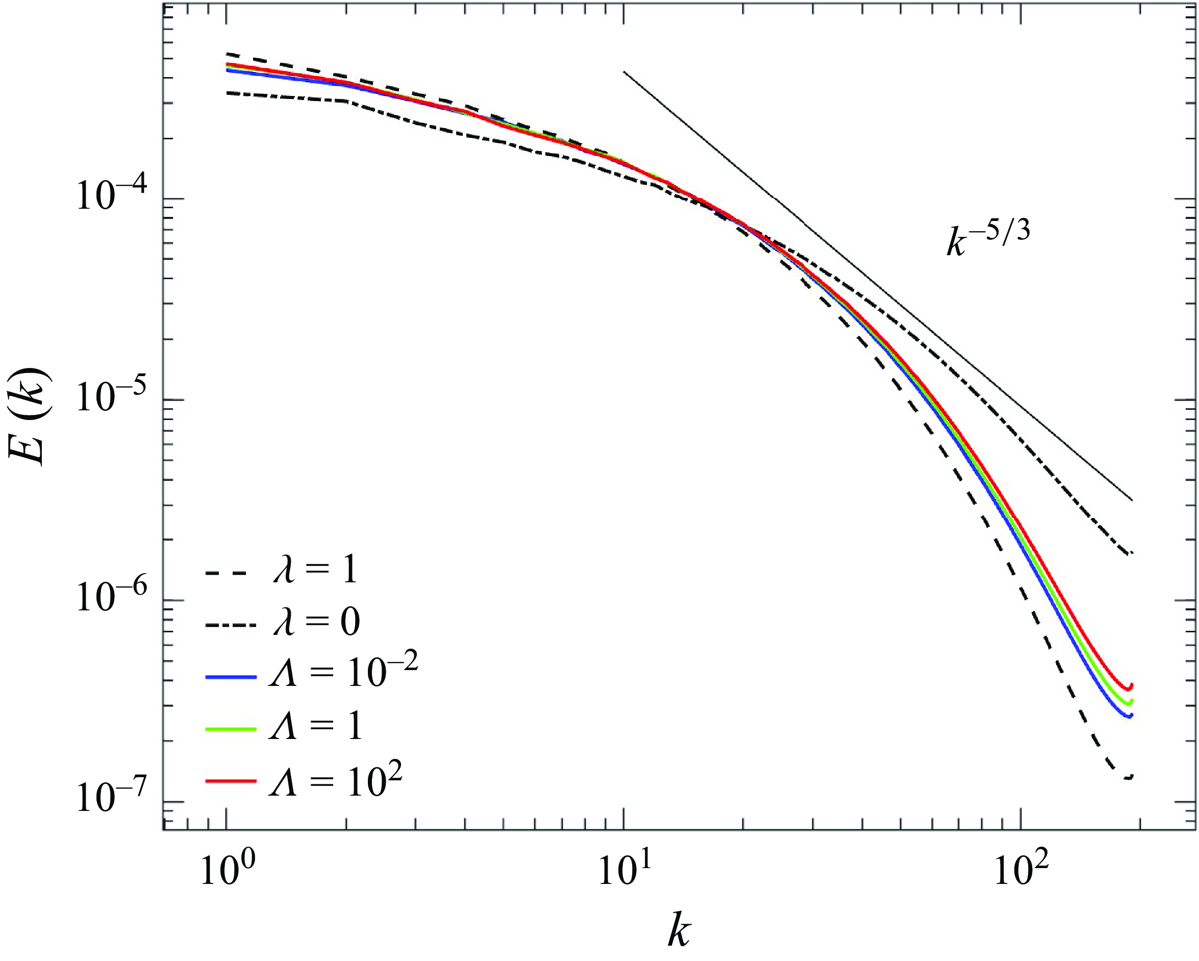
Figure 9. Modal energy spectrum $E(k)$
as a function of the wavenumber
$E(k)$
as a function of the wavenumber $k$
for thixotropic flows and Newtonian reference cases.
$k$
for thixotropic flows and Newtonian reference cases.
As figures 6–9 are based on a fixed body force $F$
, both thixotropy and inertia (as reflected by
$F$
, both thixotropy and inertia (as reflected by $Re_G$
in table 2) vary across the various models. To isolate thixotropic effects, figure 10 compares the thixotropic cases with their Newtonian counterparts at the same Reynolds number
$Re_G$
in table 2) vary across the various models. To isolate thixotropic effects, figure 10 compares the thixotropic cases with their Newtonian counterparts at the same Reynolds number $Re$
. As it is not possible to run Semtex at a known
$Re$
. As it is not possible to run Semtex at a known $Re$
a priori, the Newtonian results are obtained via the interpolation of radial profiles from Newtonian turbulent pipe flow computations at
$Re$
a priori, the Newtonian results are obtained via the interpolation of radial profiles from Newtonian turbulent pipe flow computations at $Re=5\ 928, 9\ 344, 11\ 057$
and
$Re=5\ 928, 9\ 344, 11\ 057$
and $13\ 246$
to match the
$13\ 246$
to match the $Re_G$
for
$Re_G$
for $\Lambda =10^{-2},\,1,\,10^2$
shown in table 2. Figure 10 shows that for the slow kinetics (
$\Lambda =10^{-2},\,1,\,10^2$
shown in table 2. Figure 10 shows that for the slow kinetics ( $\Lambda = 10^{-2}$
), the thixotropic rheology is close to Newtonian, hence the thixotropic and Newtonian profiles are very close match, with a relative
$\Lambda = 10^{-2}$
), the thixotropic rheology is close to Newtonian, hence the thixotropic and Newtonian profiles are very close match, with a relative $L_2$
deviation of 0.69 % for the mean velocity and up to 3.67 % for the other turbulent statistics. In contrast, the thixotropic fluid behaves similar to a shear-thinning fluid for the fast kinetics case (
$L_2$
deviation of 0.69 % for the mean velocity and up to 3.67 % for the other turbulent statistics. In contrast, the thixotropic fluid behaves similar to a shear-thinning fluid for the fast kinetics case ( $\Lambda = 10^2$
), leading to larger deviations from the Newtonian reference (up to 4.46 %), which is consistent with previous studies (Singh et al. Reference Singh, Rudman and Blackburn2017a
,Reference Singh, Rudman and Blackburn
b
). For intermediate kinetics (
$\Lambda = 10^2$
), leading to larger deviations from the Newtonian reference (up to 4.46 %), which is consistent with previous studies (Singh et al. Reference Singh, Rudman and Blackburn2017a
,Reference Singh, Rudman and Blackburn
b
). For intermediate kinetics ( $\Lambda = 1$
), the fluid is still predominantly shear-thinning and so is also qualitatively consistent with that of Singh et al. (Reference Singh, Rudman and Blackburn2017a
,Reference Singh, Rudman and Blackburn
b
).
$\Lambda = 1$
), the fluid is still predominantly shear-thinning and so is also qualitatively consistent with that of Singh et al. (Reference Singh, Rudman and Blackburn2017a
,Reference Singh, Rudman and Blackburn
b
).
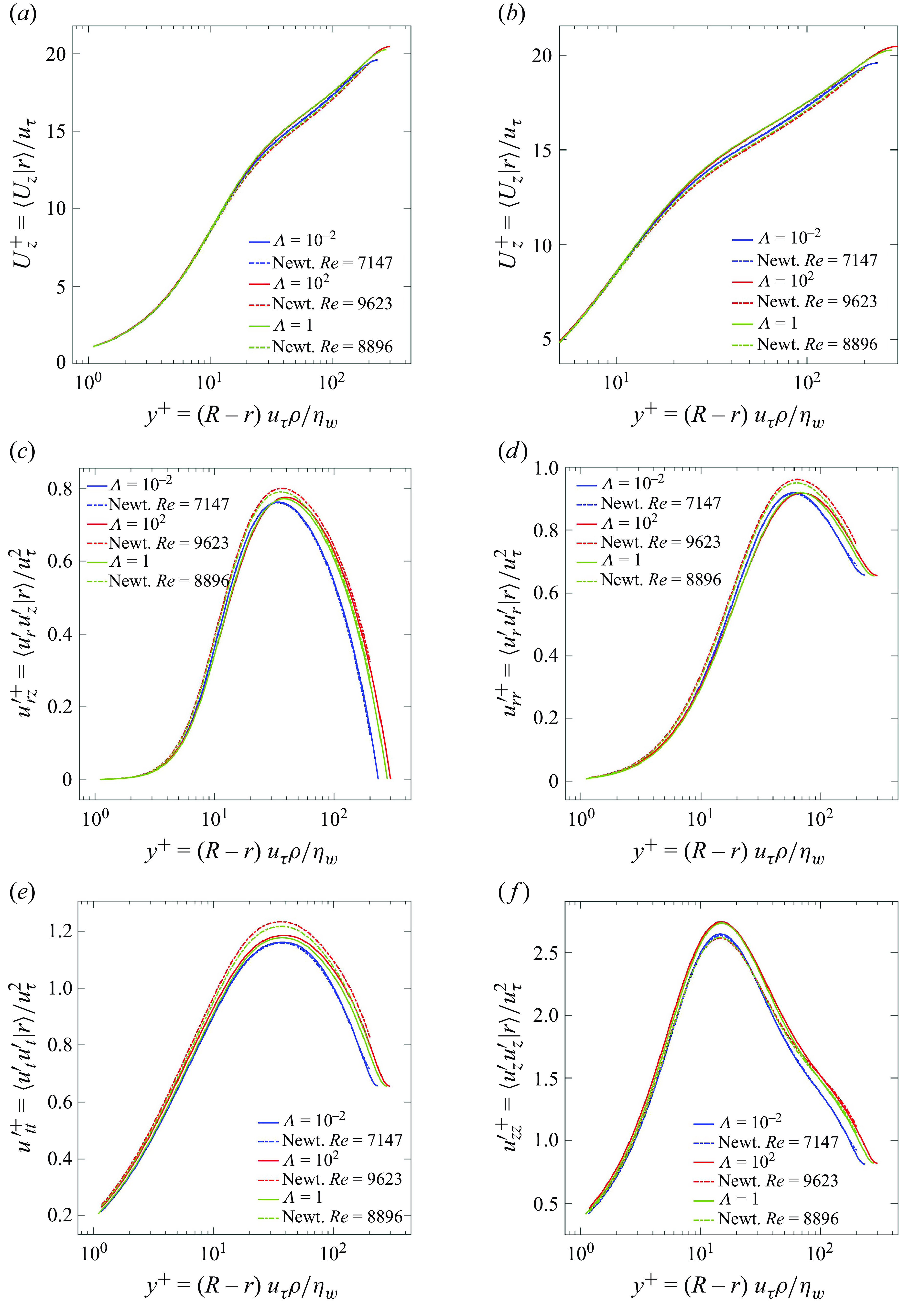
Figure 10. Radial profiles of (a–b) mean velocity and (c–f) Reynolds stresses for turbulent pipe flow of (solids lines) thixotropic fluids and (dotted lines) Newtonian fluids with Reynolds number matching the thixotropic cases. The profiles for thixotropic fluids are generated directly from DNS computations and the profiles for Newtonian fluids at matching $Re$
are interpolated from profiles at fixed
$Re$
are interpolated from profiles at fixed $Re$
.
$Re$
.
4. Lagrangian thixotropy
4.1. Lagrangian frame
The results in § 3 suggest that the shear history along pathlines plays a critical role in organizing thixotropic turbulence. As the ADRE (2.15) for $\lambda$
is advection-dominated (
$\lambda$
is advection-dominated ( $Pe\gg 1$
), the Lagrangian frame is well-suited to study the feedback mechanisms that govern thixotropic turbulence, as this naturally encodes the shear history experienced by fluid elements. In this section we develop a Lagrangian model of thixotropy that provides insights into the feedback mechanisms that govern thixotropic turbulence and use these insights to develop analogue time-independent rheological models.
$Pe\gg 1$
), the Lagrangian frame is well-suited to study the feedback mechanisms that govern thixotropic turbulence, as this naturally encodes the shear history experienced by fluid elements. In this section we develop a Lagrangian model of thixotropy that provides insights into the feedback mechanisms that govern thixotropic turbulence and use these insights to develop analogue time-independent rheological models.
We first consider evolution of the structural parameter $\lambda$
in the Lagrangian frame
$\lambda$
in the Lagrangian frame $\textbf{X}$
as
$\textbf{X}$
as $\lambda (t;\textbf{X},t_0)=\lambda (\textbf{x}(t;\textbf{X},t_0),t)$
, where
$\lambda (t;\textbf{X},t_0)=\lambda (\textbf{x}(t;\textbf{X},t_0),t)$
, where $\textbf{x}(t;\textbf{X},t_0)$
is the solution of the advection equation for a fluid particle initially at position
$\textbf{x}(t;\textbf{X},t_0)$
is the solution of the advection equation for a fluid particle initially at position $\textbf{X}$
at time
$\textbf{X}$
at time $t=t_0$
:
$t=t_0$
:
 \begin{equation} \frac {{\rm d}\textbf{x}(t;\textbf{X},t_0)}{{\rm d}t}=\textbf{v}(x(t;\textbf{X},t_0),t) ,\quad \textbf{x}(t_0;\textbf{X},t_0)=\textbf{X}. \end{equation}
In the limit of vanishing diffusivity ( $Pe \rightarrow \infty$
), the ADRE (2.15) can be transformed to the Lagrangian frame as
$Pe \rightarrow \infty$
), the ADRE (2.15) can be transformed to the Lagrangian frame as
 \begin{equation} \frac {\partial \lambda (t;\textbf{X},t_0)}{\partial t} = \Lambda \left ([1-\lambda (t;\textbf{X},t_0]-K\dot \gamma (t;\textbf{X},t_0)\lambda (t;\textbf{X},t_0))\right ) ,\quad \lambda (t_0;\textbf{X},t_0)=\lambda _0. \end{equation}
Solution of (4.2) shows that the structural parameter evolves with respect to Lagrangian shear history as
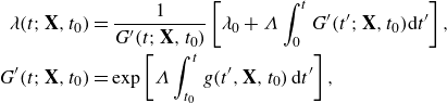 \begin{align} \lambda (t;\textbf{X},t_0)&=\frac {1}{G'(t;\textbf{X},t_0)}\left [\lambda _0+\Lambda \int _0^t G'(t^\prime ;\textbf{X},t_0){\rm d}t^\prime \right ],\nonumber\\ G'(t;\textbf{X},t_0)&=\exp \left [\Lambda \int _{t_0}^t g(t^\prime ,\textbf{X},t_0)\,{\rm d}t^\prime \right ], \end{align}
where $g(t,\textbf{X},t_0)\equiv 1+K\dot \gamma (t,\textbf{X},t_0)$
. As we are interested in the long-time behaviour of
$g(t,\textbf{X},t_0)\equiv 1+K\dot \gamma (t,\textbf{X},t_0)$
. As we are interested in the long-time behaviour of $\lambda (t)$
, given by
$\lambda (t)$
, given by $t_0\rightarrow -\infty$
(or more accurately
$t_0\rightarrow -\infty$
(or more accurately $t-t_0\gg 1/\Lambda$
), the initial condition
$t-t_0\gg 1/\Lambda$
), the initial condition $\lambda _0$
has no impact on
$\lambda _0$
has no impact on $\lambda$
and (4.3) may be recast as
$\lambda$
and (4.3) may be recast as
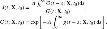 \begin{align} \lambda (t;\textbf{X},t_0)&=\frac {\Lambda \int _0^\infty G(t-s;\textbf{X},t_0){\rm d}s}{G(t;\textbf{X},t_0)},\nonumber\\ G(t;\textbf{X},t_0)&=\exp \left [-\Lambda \int _0^\infty g(t-s;\textbf{X},t_0)\,{\rm d}s\right ]. \end{align}
Here $G$
in (4.4) represents a fading memory kernel
$G$
in (4.4) represents a fading memory kernel $\hat {\mathcal{F}}$
 \begin{equation} G(t;\textbf{X},t_0)=\hat {\mathcal{F}}\left [\dot \gamma (t-s;\textbf{X},t_0)|_{s=0}^{\infty }\right ], \end{equation}
that encodes the shear history from $s=0$
to
$s=0$
to $s\rightarrow -\infty$
. Hence the most recent shear rates have the greatest impact, and the persistence of memory (analogous to relaxation time for viscoelastic fluids) is controlled by the thixoviscous number.
$s\rightarrow -\infty$
. Hence the most recent shear rates have the greatest impact, and the persistence of memory (analogous to relaxation time for viscoelastic fluids) is controlled by the thixoviscous number.
Equations (4.4) and (4.5) also show that advective transport is an important mechanism in non-stationary thixotropic turbulent flow. From a stochastic perspective, the Lagrangian shear rate history $\dot \gamma (t-s;\textbf{X},t_0)$
can be considered as a random process that is non-stationary in space and so is also dependent upon the history
$\dot \gamma (t-s;\textbf{X},t_0)$
can be considered as a random process that is non-stationary in space and so is also dependent upon the history $s$
of Eulerian positions
$s$
of Eulerian positions $\textbf{x}(t-s;\textbf{X},t_0)$
along pathlines. For fully developed turbulent pipe flow the shear rate
$\textbf{x}(t-s;\textbf{X},t_0)$
along pathlines. For fully developed turbulent pipe flow the shear rate $\dot \gamma$
is non-stationary in the radial direction
$\dot \gamma$
is non-stationary in the radial direction $r$
, hence the functional (4.5) simplifies to
$r$
, hence the functional (4.5) simplifies to $G(r(t),t)=\hat {\mathcal{F}}[\dot \gamma (t-s;r(t-s))|_{s=0}^{\infty }]$
, and the evolution equation (4.4) needs to be supplemented by an advective transport model for evolution of radial position
$G(r(t),t)=\hat {\mathcal{F}}[\dot \gamma (t-s;r(t-s))|_{s=0}^{\infty }]$
, and the evolution equation (4.4) needs to be supplemented by an advective transport model for evolution of radial position $r(t)$
. This stochastic approach will be considered further in § 5.2.
$r(t)$
. This stochastic approach will be considered further in § 5.2.
Conversely, for statistically stationary turbulent flows (4.5) simplifies to $G(t)=\hat {\mathcal{F}}[\dot \gamma (t-s)|_{s=0}^{\infty }$
. If the Lagrangian shear rate follows a simple autocorrelation process with decorrelation time
$G(t)=\hat {\mathcal{F}}[\dot \gamma (t-s)|_{s=0}^{\infty }$
. If the Lagrangian shear rate follows a simple autocorrelation process with decorrelation time $\tau _{\dot \gamma }$
,
$\tau _{\dot \gamma }$
,
 \begin{align} R_{\dot \gamma \dot \gamma }(|t-t^\prime |)\equiv \langle \dot \gamma ^\prime (t;\textbf{X},t_0)\dot \gamma ^\prime (t^\prime ;\textbf{X},t_0)\rangle \sim \exp \left (-|t-t^\prime |/\tau _{\dot \gamma }\right ), \end{align}
then $\dot \gamma (t-s)$
may be modelled as a Markovian random process, leading to a fairly simple random walk model for the evolution of
$\dot \gamma (t-s)$
may be modelled as a Markovian random process, leading to a fairly simple random walk model for the evolution of $\lambda$
via (4.4).
$\lambda$
via (4.4).
To test the Lagrangian assumption, the evolution of $\lambda$
along different pathlines is compared in figure 11 between DNS results and computation of
$\lambda$
along different pathlines is compared in figure 11 between DNS results and computation of $\lambda$
via in (4.2). For the fast thixotropic kinetics (
$\lambda$
via in (4.2). For the fast thixotropic kinetics ( $\Lambda = 10^2$
) with a high Damköhler number (
$\Lambda = 10^2$
) with a high Damköhler number ( $Da = 10^5$
), the DNS results closely match the Lagrangian solution (4.2), with a relative
$Da = 10^5$
), the DNS results closely match the Lagrangian solution (4.2), with a relative $L_2$
error of 0.18 % over
$L_2$
error of 0.18 % over $10^4$
trajectories. For intermediate kinetics (
$10^4$
trajectories. For intermediate kinetics ( $\Lambda =1$
), diffusion is significant although thixotropic kinetics still dominate (
$\Lambda =1$
), diffusion is significant although thixotropic kinetics still dominate ( $Da = 10^3$
), and the Lagrangian solution (4.2) has relative
$Da = 10^3$
), and the Lagrangian solution (4.2) has relative $L_2$
error of 1.79 %. For the slow kinetics (
$L_2$
error of 1.79 %. For the slow kinetics ( $\Lambda = 10^{-2}$
), the time scales of diffusion approach those of the thixotropic kinetics (
$\Lambda = 10^{-2}$
), the time scales of diffusion approach those of the thixotropic kinetics ( $Da = 10$
), leading to noticeable discrepancies in pathlines and relative
$Da = 10$
), leading to noticeable discrepancies in pathlines and relative $L_2$
error of 4.03 %. The discrepancies in figure 11(c) are due to the moderate Péclet number (
$L_2$
error of 4.03 %. The discrepancies in figure 11(c) are due to the moderate Péclet number ( $Pe=10^3$
) used for numerical stability, corresponding to
$Pe=10^3$
) used for numerical stability, corresponding to $Da\sim 10$
for
$Da\sim 10$
for $\Lambda =10^{-2}$
. As previously discussed, both
$\Lambda =10^{-2}$
. As previously discussed, both $Pe$
and
$Pe$
and $Da$
are much higher for complex fluids, hence the Lagrangian framework is broadly applicable to thixotropic flows. Although the Lagrangian assumption does not strictly hold in this study for
$Da$
are much higher for complex fluids, hence the Lagrangian framework is broadly applicable to thixotropic flows. Although the Lagrangian assumption does not strictly hold in this study for $\Lambda \ll 1$
, we shall show in the following that this does not significantly alter the overall dynamics of the flow, and accurate analytic closures for the limiting cases of
$\Lambda \ll 1$
, we shall show in the following that this does not significantly alter the overall dynamics of the flow, and accurate analytic closures for the limiting cases of $\Lambda$
can be developed.
$\Lambda$
can be developed.
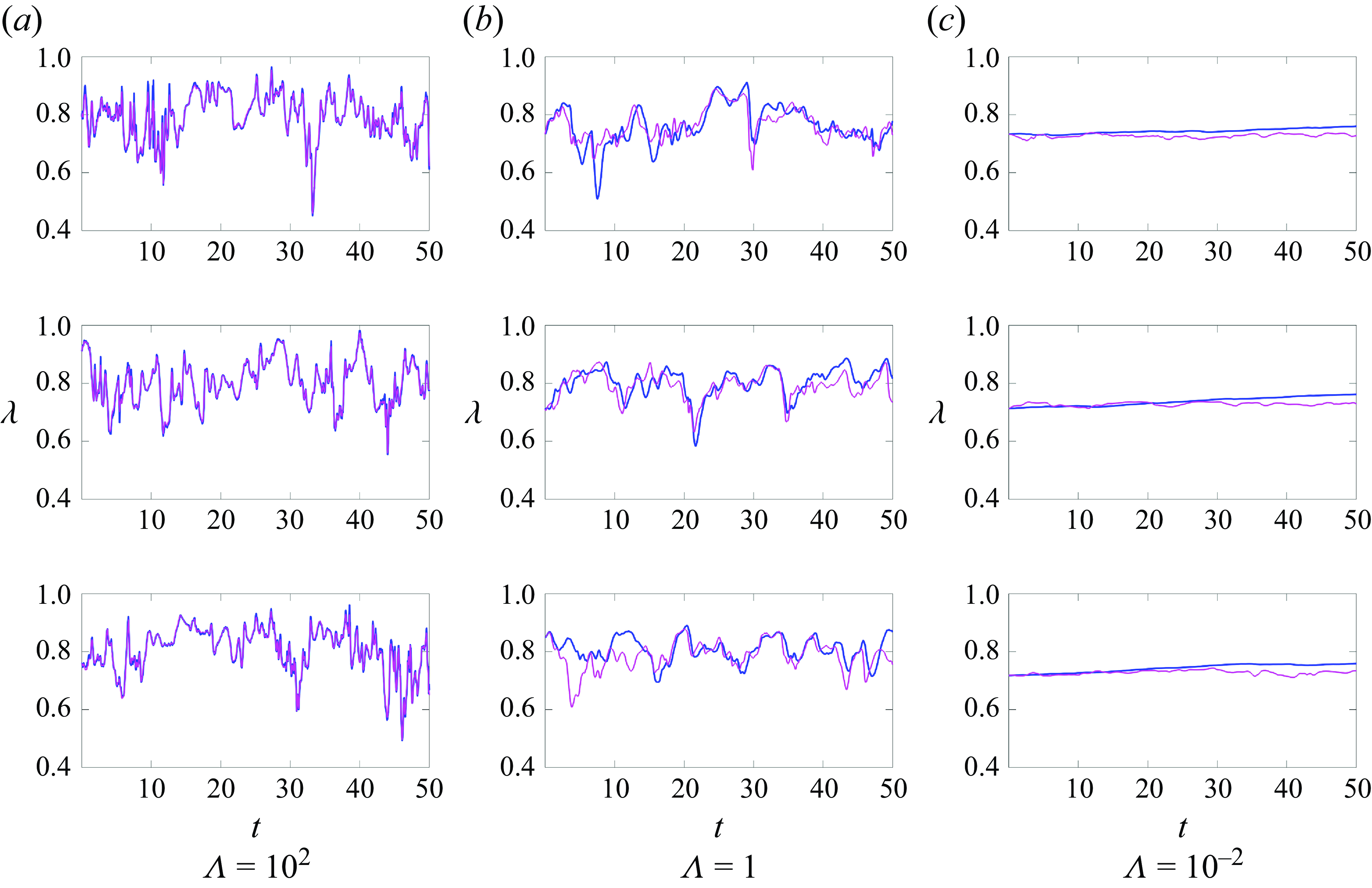
Figure 11. Comparison of structural parameter $\lambda (t;\textbf{X},t_0)$
along representative particle trajectories at
$\lambda (t;\textbf{X},t_0)$
along representative particle trajectories at $r\sim 0.4$
(near the pipe walls) for thixotropic flows with (a)
$r\sim 0.4$
(near the pipe walls) for thixotropic flows with (a) $\Lambda =10^{2}$
, (b)
$\Lambda =10^{2}$
, (b) $\Lambda =1$
and (c)
$\Lambda =1$
and (c) $\Lambda =10^{-2}$
, from (
$\Lambda =10^{-2}$
, from (
![]() ) DNS results and (
) DNS results and (
![]() ) solution of the Lagrangian equation (4.2).
) solution of the Lagrangian equation (4.2).
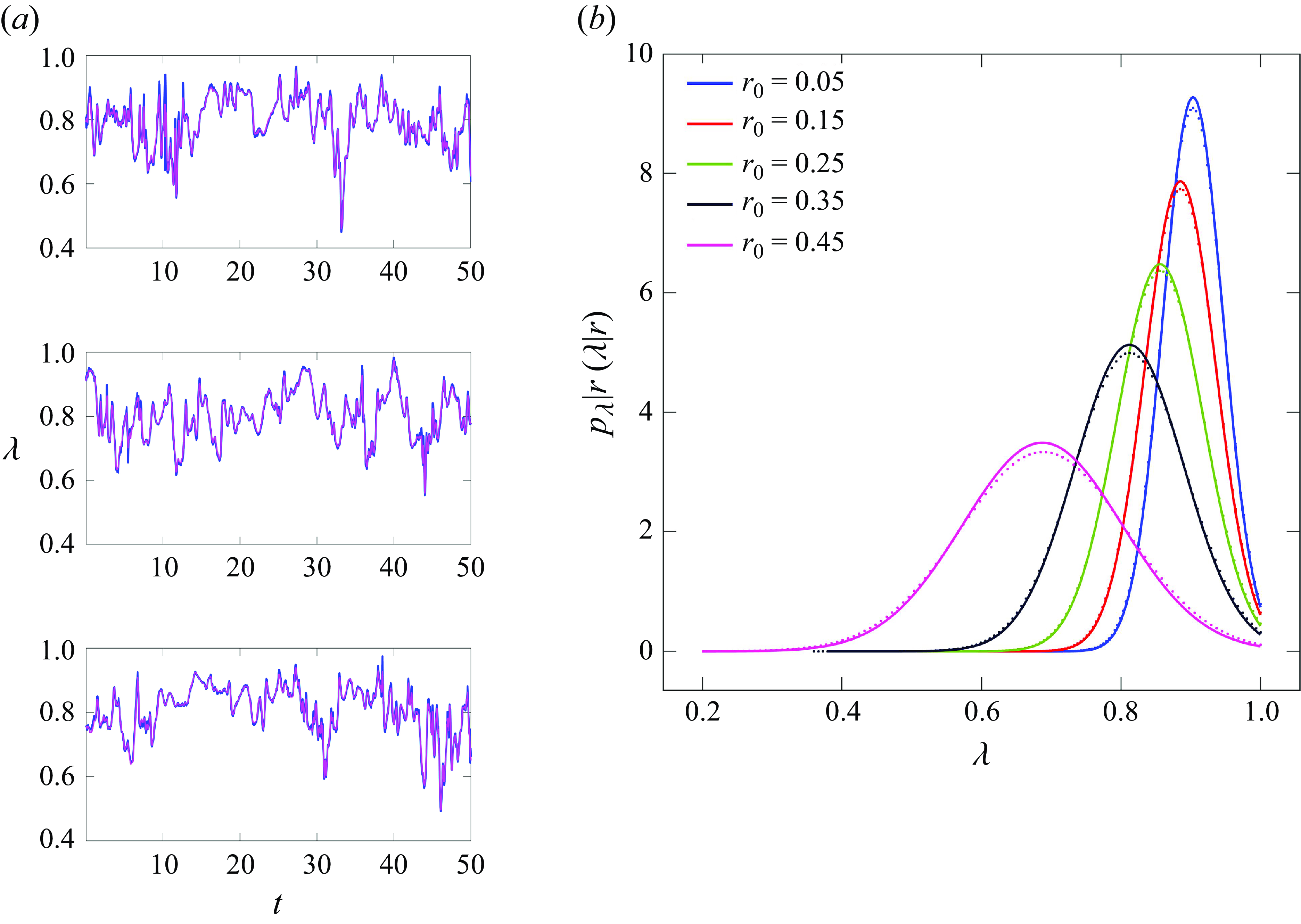
Figure 12. (a) Comparison of structural parameter $\lambda (t;\textbf{X},t_0)$
along representative particle trajectories at
$\lambda (t;\textbf{X},t_0)$
along representative particle trajectories at $r\sim 0.4$
(near the pipe walls) for thixotropic flows with
$r\sim 0.4$
(near the pipe walls) for thixotropic flows with $\Lambda =10^{2}$
, from (
$\Lambda =10^{2}$
, from (
![]() ) DNS results and (
) DNS results and (
![]() ) the analytic closure (4.10). (b) Comparison of conditional p.d.f. of structural parameter
) the analytic closure (4.10). (b) Comparison of conditional p.d.f. of structural parameter $p_\lambda (\lambda |r)$
along typical particle trajectories for thixotropic flows with
$p_\lambda (\lambda |r)$
along typical particle trajectories for thixotropic flows with $\Lambda =10^{2}$
, from (solid lines) DNS results and (dotted lines) the analytic closure (4.10).
$\Lambda =10^{2}$
, from (solid lines) DNS results and (dotted lines) the analytic closure (4.10).
4.2. Fast kinetics
In the fast kinetic regime, $\Lambda \gg 1$
, the thixotropic time scale
$\Lambda \gg 1$
, the thixotropic time scale $\tau _r$
is much shorter than the eddy turnover time
$\tau _r$
is much shorter than the eddy turnover time $\tau _v$
that governs the Lagrangian shear rate decorrelation time, hence only the very recent shear history dictates
$\tau _v$
that governs the Lagrangian shear rate decorrelation time, hence only the very recent shear history dictates $\lambda$
. Following (4.4), we derive an expression for the structural parameter
$\lambda$
. Following (4.4), we derive an expression for the structural parameter $\lambda$
in the limit
$\lambda$
in the limit $\Lambda \gg 1$
by first performing a series expansion of
$\Lambda \gg 1$
by first performing a series expansion of $\dot \gamma (t-s;\textbf{X},t_0)$
about
$\dot \gamma (t-s;\textbf{X},t_0)$
about $t$
as
$t$
as
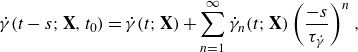 \begin{equation} \dot \gamma (t-s;\textbf{X},t_0)=\dot \gamma (t;\textbf{X})+\sum _{n=1}^\infty \dot \gamma _n(t;\textbf{X})\left (\frac {-s}{\tau _{\dot \gamma }}\right )^n, \end{equation}
where from the definition of $\tau _{\dot \gamma }$
, the coefficients
$\tau _{\dot \gamma }$
, the coefficients $\dot \gamma _n(t;\textbf{X},t_0)\equiv \dot \gamma (t;\textbf{X},t_0)^{(n)}\tau _{\dot \gamma }^n/n!\sim 1$
, and
$\dot \gamma _n(t;\textbf{X},t_0)\equiv \dot \gamma (t;\textbf{X},t_0)^{(n)}\tau _{\dot \gamma }^n/n!\sim 1$
, and $x^{(n)}(t)$
denotes the
$x^{(n)}(t)$
denotes the $n$
th derivative of
$n$
th derivative of $x$
with respect to
$x$
with respect to $t$
. Introducing the rescaled thixotropic time
$t$
. Introducing the rescaled thixotropic time $t_r=t\Lambda$
, the structural parameter evolves according to
$t_r=t\Lambda$
, the structural parameter evolves according to
 \begin{equation} \lim _{\Lambda \rightarrow \infty }\lambda (t;\textbf{X},t_0)=\lim _{\Lambda \rightarrow \infty }\lambda (t_r/\Lambda ;\textbf{X},t_0)=\frac {\lim _{\Lambda \rightarrow \infty }\int _{t_0}^{r/\Lambda }G\left (t_r/\Lambda ;\textbf{X},t_0\right ){\rm d}t_r}{\lim _{\Lambda \rightarrow \infty }G\left (t_r/\Lambda ;\textbf{X},t_0\right )} \end{equation}
where the history function $G(t;\textbf{X},t_0)$
in the limit
$G(t;\textbf{X},t_0)$
in the limit $\Lambda \gg 1$
is then
$\Lambda \gg 1$
is then
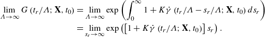 \begin{align} \lim _{\Lambda \rightarrow \infty }G\left (t_r/\Lambda ;\textbf{X},t_0\right )=&\lim _{\Lambda \rightarrow \infty }\exp \left (\int _0^\infty 1+K\dot \gamma \left (t_r/\Lambda -s_r/\Lambda ;\textbf{X},t_0\right )ds_r\right )\nonumber\\ =&\lim _{s_r\rightarrow \infty }\exp \left (\left [1+K\dot \gamma \left (t_r/\Lambda ;\textbf{X},t_0\right )\right ]s_r\right ). \end{align}
Application of L’Hopital’s rule to (4.8) yields
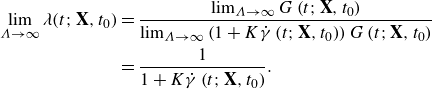 \begin{align} \lim _{\Lambda \rightarrow \infty }\lambda (t;\textbf{X},t_0) & =\frac {\lim _{\Lambda \rightarrow \infty }G\left (t;\textbf{X},t_0\right )}{\lim _{\Lambda \rightarrow \infty }\left (1+K\dot \gamma \left (t;\textbf{X},t_0\right )\right )G\left (t;\textbf{X},t_0\right )} \nonumber\\ & = \frac {1}{1+K\dot \gamma \left (t;\textbf{X},t_0\right )}. \end{align}
Hence, the structural parameter in Eulerian space for $\Lambda \gg 1$
is given by the equilibrium value
$\Lambda \gg 1$
is given by the equilibrium value
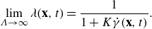 \begin{equation} \lim _{\Lambda \rightarrow \infty }\lambda (\textbf{x},t)=\frac {1}{1+K\dot \gamma (\textbf{x},t)}. \end{equation}
For $\Lambda \gg 1$
the structural parameter instantly equilibrates with respect to the local shear rate, hence the effective viscosity of the thixotropic psuedo-Newtonian fluid is a time-independent shear-thinning GN fluid (Scott-Blair Reference Scott-Blair1951; Barnes Reference Barnes1997) that corresponds to a Cross fluid with unit index
$\Lambda \gg 1$
the structural parameter instantly equilibrates with respect to the local shear rate, hence the effective viscosity of the thixotropic psuedo-Newtonian fluid is a time-independent shear-thinning GN fluid (Scott-Blair Reference Scott-Blair1951; Barnes Reference Barnes1997) that corresponds to a Cross fluid with unit index
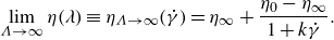 \begin{equation} \lim _{\Lambda \rightarrow \infty }\eta (\lambda )\equiv \eta _{\Lambda \rightarrow \infty }(\dot \gamma )=\eta _\infty +\frac {\eta _0-\eta _\infty }{1+k\dot \gamma } . \end{equation}
Figure 12 verifies (4.10) via comparison with DNS computations for $\Lambda = 10^2$
. Figure 12(a) shows that the fast kinetics model (4.10) for evolution of
$\Lambda = 10^2$
. Figure 12(a) shows that the fast kinetics model (4.10) for evolution of $\lambda$
along sample trajectories matches DNS results very well, with a relative
$\lambda$
along sample trajectories matches DNS results very well, with a relative $L_2$
error of 0.1 % across
$L_2$
error of 0.1 % across $10^4$
Lagrangian trajectories. Figure 12(b) also shows that the conditional probability density function (p.d.f.) of
$10^4$
Lagrangian trajectories. Figure 12(b) also shows that the conditional probability density function (p.d.f.) of $\lambda$
at various radial positions
$\lambda$
at various radial positions $p_{\lambda |r}(\lambda |r)$
from (4.10) also matches the DNS results very well, verifying both the Lagrangian assumption and the closure model (4.10).
$p_{\lambda |r}(\lambda |r)$
from (4.10) also matches the DNS results very well, verifying both the Lagrangian assumption and the closure model (4.10).
To test the closure (4.10) and the corresponding effective viscosity model (4.12), DNS computations using (4.12) are compared with those using the thixotropic kinetics with $\Lambda =10^2$
in figures 6–8. Computations based on the effective viscosity model (4.12) show excellent agreement with the full thixotropic model, with relative errors of under 0.1% for the mean structural parameter
$\Lambda =10^2$
in figures 6–8. Computations based on the effective viscosity model (4.12) show excellent agreement with the full thixotropic model, with relative errors of under 0.1% for the mean structural parameter $\lambda$
, viscosity
$\lambda$
, viscosity $\eta$
and axial velocity
$\eta$
and axial velocity $U_z$
. The errors in turbulent statistics (
$U_z$
. The errors in turbulent statistics ( $u'_{rr},u'_{tt},u'_{zz},u'_{rz}$
) are also all less than 0.5 %. Figures 2 and 3 also show that the closure (4.10) closely matches the fully thixotropic model in the limit
$u'_{rr},u'_{tt},u'_{zz},u'_{rz}$
) are also all less than 0.5 %. Figures 2 and 3 also show that the closure (4.10) closely matches the fully thixotropic model in the limit $\Lambda \gg 1$
, and the difference in the structural parameter fields are of small magnitude and high wavenumber due to Lagrangian shear rate fluctuations perturbing
$\Lambda \gg 1$
, and the difference in the structural parameter fields are of small magnitude and high wavenumber due to Lagrangian shear rate fluctuations perturbing $\lambda$
away from the equilibrium value (4.10). Note that these perturbations are more pronounced near the wall where the fluctuations in shear rate are greatest. These results confirm that, as expected, for
$\lambda$
away from the equilibrium value (4.10). Note that these perturbations are more pronounced near the wall where the fluctuations in shear rate are greatest. These results confirm that, as expected, for $\Lambda \gg 1$
thixotropic fluids exhibit turbulent fluid dynamics akin to that of shear-thinning fluids. Note that this result extends to a broad range of rheologies and thixotropic models described by (2.3) and (2.5), respectively.
$\Lambda \gg 1$
thixotropic fluids exhibit turbulent fluid dynamics akin to that of shear-thinning fluids. Note that this result extends to a broad range of rheologies and thixotropic models described by (2.3) and (2.5), respectively.
4.3. Slow kinetics
To analyse thixotropic rheology in the limit of vanishingly slow thixotropic kinetics, $\Lambda \ll 1$
, we decompose the memory kernel into an ensemble average
$\Lambda \ll 1$
, we decompose the memory kernel into an ensemble average $\langle \dot \gamma \rangle$
that, due to ergodicity, corresponds to the Lagrangian average
$\langle \dot \gamma \rangle$
that, due to ergodicity, corresponds to the Lagrangian average
 \begin{equation} \langle \dot \gamma \rangle \equiv \int _{-\infty }^\infty \dot \gamma p_{\dot \gamma }(\dot \gamma ) {\rm d}\dot \gamma = \lim _{T\rightarrow \infty }\frac {1}{T}\int _0^T\dot \gamma (t;\textbf{X},t_0){\rm d}t, \end{equation}
and a fluctuating component $\dot \gamma '$
as
$\dot \gamma '$
as
 \begin{equation} \dot \gamma (t;\textbf{X},t_0)=\langle \dot \gamma \rangle +\dot \gamma '(t/\tau _{\dot \gamma };\textbf{X},t_0), \end{equation}
where the scaling $t/\tau _{\dot \gamma }$
ensures
$t/\tau _{\dot \gamma }$
ensures $\partial \dot \gamma '/\partial t\sim 1$
. Using this decomposition, the memory kernel (4.4) is then
$\partial \dot \gamma '/\partial t\sim 1$
. Using this decomposition, the memory kernel (4.4) is then
 \begin{align} G(t;\textbf{X},t_0)&=\exp \left (\Lambda \int _{t_0}^t 1+K\langle \dot \gamma \rangle +K\dot \gamma '(t/\tau _{\dot \gamma };\textbf{X},t_0) {\rm d}t^\prime \right )\nonumber\\ &=\exp \left (\Lambda (1+K\langle \dot \gamma \rangle )(t-t_0)\right )\exp \left (\Lambda K\int _{t_0}^t\dot \gamma '(t/\tau _{\dot \gamma };\textbf{X},t_0) {\rm d}t^\prime \right ). \end{align}
and integration by parts yields
 \begin{align} \Lambda \int _{t_0}^t G(t^\prime ;\textbf{X},t_0){\rm d}t^\prime & =\frac {G(t^\prime ;\textbf{X},t_0)-1}{1+K\langle \dot \gamma \rangle }- \Lambda \int _{t_0 \tau _{\dot \gamma }}^{t \tau _{\dot \gamma }}\frac {K\dot \gamma '(t_2^\prime ;\textbf{X},t_0)}{1+K\langle \dot \gamma \rangle }G(t_2^\prime \tau _{\dot \gamma };\textbf{X},t_0) {\rm d}t_2^\prime , \end{align}
where $t_2=t \tau _{\dot \gamma }$
. In the limits
$t_2=t \tau _{\dot \gamma }$
. In the limits $t_0\rightarrow -\infty$
,
$t_0\rightarrow -\infty$
, $\Lambda \ll 1$
, the structural parameter given by (4.4) then simplifies to
$\Lambda \ll 1$
, the structural parameter given by (4.4) then simplifies to
 \begin{equation} \lim _{\Lambda \rightarrow 0}\lambda (t;\textbf{X},t_0)=\frac {1}{1+K\langle \dot \gamma \rangle }=\lim _{\Lambda \rightarrow 0}\lambda (t,\textbf{x}). \end{equation}
Hence, for $\Lambda \ll 1$
, the thixotropic kinetics are so slow compared to the fluctuation rate of the shear rate that the structural parameter effectively samples the ensemble of shear rates during convergence to equilibrium, and so the structural parameter is steady and is governed by the ensemble averaged shear rate
$\Lambda \ll 1$
, the thixotropic kinetics are so slow compared to the fluctuation rate of the shear rate that the structural parameter effectively samples the ensemble of shear rates during convergence to equilibrium, and so the structural parameter is steady and is governed by the ensemble averaged shear rate $\langle \dot \gamma \rangle$
. Hence, the structural parameter in Eulerian space for
$\langle \dot \gamma \rangle$
. Hence, the structural parameter in Eulerian space for $\Lambda \ll 1$
is given by the equilibrium value at the mean shear rate as
$\Lambda \ll 1$
is given by the equilibrium value at the mean shear rate as
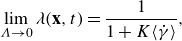 \begin{equation} \lim _{\Lambda \rightarrow 0}\lambda (\textbf{x},t)=\frac {1}{1+K \langle \dot {\gamma }\rangle }, \end{equation}
and so the thixotropic viscosity for $\Lambda \ll 1$
simplifies to the Newtonian viscosity
$\Lambda \ll 1$
simplifies to the Newtonian viscosity
 \begin{equation} \lim _{\Lambda \rightarrow 0}\eta (\lambda )\equiv \eta _{\Lambda \rightarrow 0}=\eta _\infty +\frac {\eta _0-\eta _\infty }{1+K\langle \dot \gamma \rangle } ,\quad \eta _\infty \leqslant \eta _{\Lambda \rightarrow 0}\leqslant \eta _0. \end{equation}
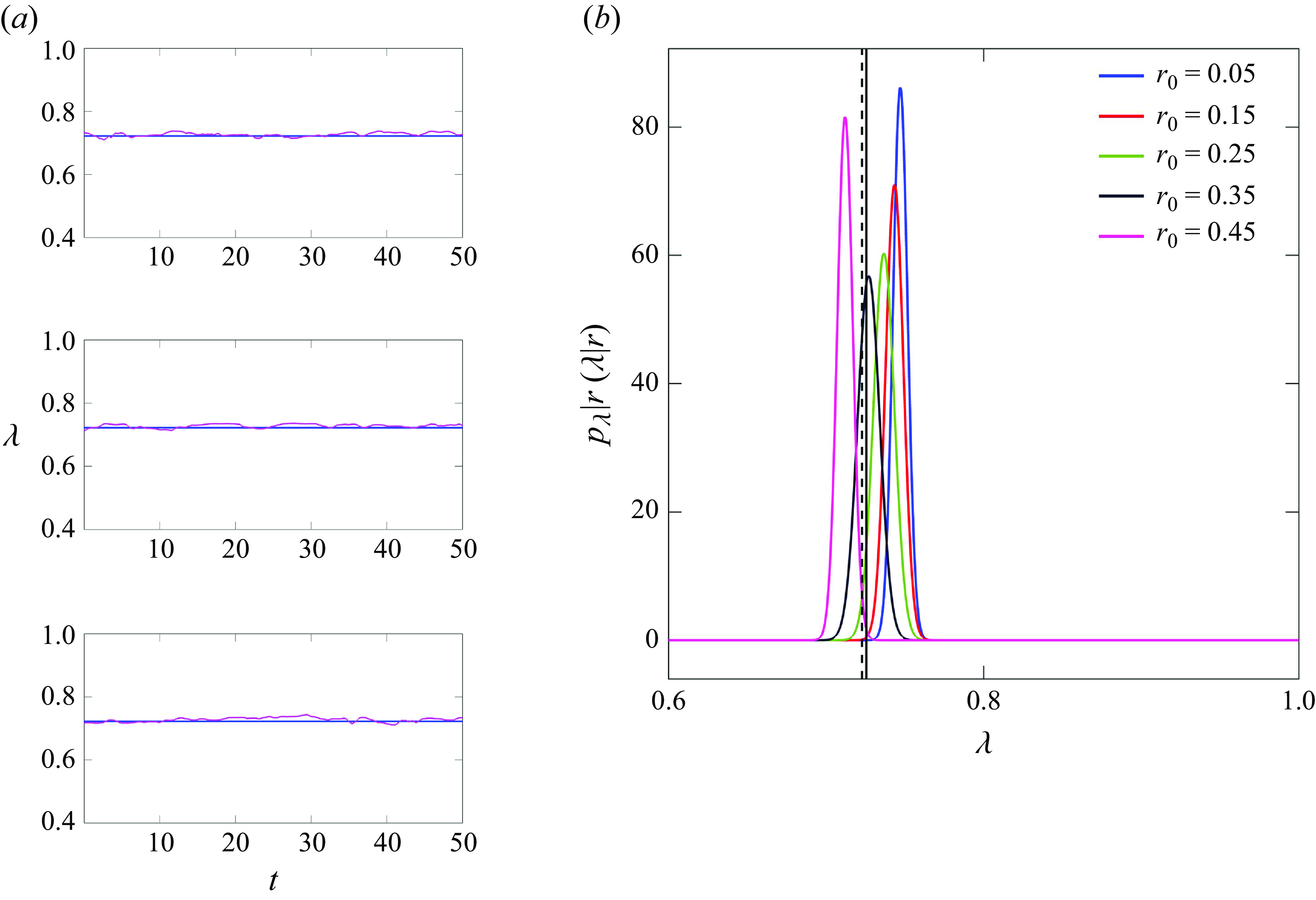
Figure 13. (a) Comparison of structural parameter $\lambda (t;\textbf{X},t_0)$
along representative particle trajectories at
$\lambda (t;\textbf{X},t_0)$
along representative particle trajectories at $r\sim 0.4$
(near the pipe walls) for thixotropic flows with
$r\sim 0.4$
(near the pipe walls) for thixotropic flows with $\Lambda =10^{-2}$
, from (
$\Lambda =10^{-2}$
, from (
![]() ) DNS results and (
) DNS results and (
![]() ) the analytic closure (4.17). (b) Comparison of conditional p.d.f. of structural parameter
) the analytic closure (4.17). (b) Comparison of conditional p.d.f. of structural parameter $p_\lambda (\lambda |r)$
along typical particle trajectories for thixotropic flows with
$p_\lambda (\lambda |r)$
along typical particle trajectories for thixotropic flows with $\Lambda =10^{-2}$
, from (solid lines) DNS results with (solid vertical line) its mean value, and (dotted line) the analytic closure (4.17).
$\Lambda =10^{-2}$
, from (solid lines) DNS results with (solid vertical line) its mean value, and (dotted line) the analytic closure (4.17).
Figure 13 verifies the slow kinetics analytic closure (4.17) by comparison with DNS computations for $\Lambda = 10^{-2}$
. Despite that the Lagrangian framework does not strictly apply for this case, figure 13(a) shows that time-series of
$\Lambda = 10^{-2}$
. Despite that the Lagrangian framework does not strictly apply for this case, figure 13(a) shows that time-series of $\lambda$
values along sample trajectories computed via DNS fluctuate close to the equilibrium value given by (4.17), with a relative
$\lambda$
values along sample trajectories computed via DNS fluctuate close to the equilibrium value given by (4.17), with a relative $L_2$
error of 1.08 % across
$L_2$
error of 1.08 % across $10^4$
Lagrangian trajectories. Similarly, figure 13(b) shows that the conditional p.d.f.
$10^4$
Lagrangian trajectories. Similarly, figure 13(b) shows that the conditional p.d.f. $p_{\lambda |r}(\lambda |r)$
from the DNS computations at different radial positions
$p_{\lambda |r}(\lambda |r)$
from the DNS computations at different radial positions $r$
all have small variance around the equilibrium value given by (4.17). These results show that despite breakdown of the Lagrangian approximation (4.2) for
$r$
all have small variance around the equilibrium value given by (4.17). These results show that despite breakdown of the Lagrangian approximation (4.2) for $\Lambda \ll 1$
due to significant diffusion of
$\Lambda \ll 1$
due to significant diffusion of $\lambda$
(i.e.
$\lambda$
(i.e. $Da=10$
), the slow kinetics closure (4.17) is still accurate as the sampling of shear rates that governs convergence of
$Da=10$
), the slow kinetics closure (4.17) is still accurate as the sampling of shear rates that governs convergence of $\dot \gamma (t;\textbf{X},t_0)\rightarrow \langle \dot \gamma \rangle$
in (4.17) is not affected by the diffusivity of
$\dot \gamma (t;\textbf{X},t_0)\rightarrow \langle \dot \gamma \rangle$
in (4.17) is not affected by the diffusivity of $\lambda$
.
$\lambda$
.
To test the closure (4.17) and the corresponding effective viscosity model (4.19), DNS computations using (4.19) are compared with those using the thixotropic kinetics with $\Lambda =10^{-2}$
in figures 6–8. Computations based on the effective viscosity model (4.19) show good agreement with the full thixotropic model, with relative errors of 2.24 % for the mean structural parameter
$\Lambda =10^{-2}$
in figures 6–8. Computations based on the effective viscosity model (4.19) show good agreement with the full thixotropic model, with relative errors of 2.24 % for the mean structural parameter $\lambda$
, 0.95 % for the mean viscosity
$\lambda$
, 0.95 % for the mean viscosity $\eta$
and 0.29 % for the axial velocity
$\eta$
and 0.29 % for the axial velocity $U_z$
. The slightly higher errors than for the fast kinetics closure may be partially due to breakdown of the Lagrangian approximation in the slow kinetics case. The errors in turbulent statistics (
$U_z$
. The slightly higher errors than for the fast kinetics closure may be partially due to breakdown of the Lagrangian approximation in the slow kinetics case. The errors in turbulent statistics ( $u'_{rr},u'_{tt},u'_{zz},u'_{rz}$
) are also all less than 0.7%. Figures 2 and 3 also show that the Newtonian closure (4.17) closely matches the fully thixotropic model in the limit
$u'_{rr},u'_{tt},u'_{zz},u'_{rz}$
) are also all less than 0.7%. Figures 2 and 3 also show that the Newtonian closure (4.17) closely matches the fully thixotropic model in the limit $\Lambda \ll 1$
, and the difference in the structural parameter fields are large length scale due to the Lagrangian averaging process. Note that the closure (4.17), respectively, over predictsand underpredicts the structural parameter
$\Lambda \ll 1$
, and the difference in the structural parameter fields are large length scale due to the Lagrangian averaging process. Note that the closure (4.17), respectively, over predictsand underpredicts the structural parameter $\lambda$
at the pipe core and wall where the local shear rate is, respectively, lower and higher than the average
$\lambda$
at the pipe core and wall where the local shear rate is, respectively, lower and higher than the average $\langle \dot \gamma \rangle$
. These results confirm that, as expected, for
$\langle \dot \gamma \rangle$
. These results confirm that, as expected, for $\Lambda \ll 1$
thixotropic fluids exhibit turbulent flow akin to that of a Newtonian fluid. Note that this result extends to a broad range of rheologies and thixotropic models described by (2.3) and (2.5), respectively.
$\Lambda \ll 1$
thixotropic fluids exhibit turbulent flow akin to that of a Newtonian fluid. Note that this result extends to a broad range of rheologies and thixotropic models described by (2.3) and (2.5), respectively.
5. Thixotropic turbulence as a non-stationary random walk
In § 4 we developed a Lagrangian framework for evolution of the structural parameter, and used this framework to establish convergence of the thixotropic rheology to the shear thinning (4.12) and Newtonian (4.19) models, respectively, in the limits of fast ( $\Lambda \gg 1$
) and slow (
$\Lambda \gg 1$
) and slow ( $\Lambda \ll 1$
) thixotropic kinetics. In this section we extend the Lagrangian framework to the case of intermediate thixotropic kinetics (
$\Lambda \ll 1$
) thixotropic kinetics. In this section we extend the Lagrangian framework to the case of intermediate thixotropic kinetics ( $\Lambda \sim 1$
) via development of a stochastic model for the Lagrangian shear history experienced by fluid elements. This stochastic model yields a rheological model for the effective viscosity that is accurate for arbitrary thixoviscous numbers
$\Lambda \sim 1$
) via development of a stochastic model for the Lagrangian shear history experienced by fluid elements. This stochastic model yields a rheological model for the effective viscosity that is accurate for arbitrary thixoviscous numbers $\Lambda \in (0,\infty ^+)$
.
$\Lambda \in (0,\infty ^+)$
.
5.1. Stochastic thixotropy as a path integral
As discussed in § 2, fully developed turbulent pipe flow is radially non-stationary, hence the random process governing the Lagrangian shear rate history $\dot \gamma (t-s;\textbf{X},t_0)$
is also radially non-stationary. Specifically, the microstructural evolution equation (4.4) may be expressed as
$\dot \gamma (t-s;\textbf{X},t_0)$
is also radially non-stationary. Specifically, the microstructural evolution equation (4.4) may be expressed as
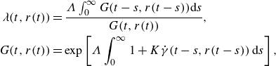 \begin{align} \lambda (t,r(t))&=\frac {\Lambda \int _0^\infty G(t-s,r(t-s)){\rm d}s}{G(t,r(t))},\nonumber\\ G(t,r(t))&=\exp \left [\Lambda \int _0^\infty 1+K\dot \gamma (t-s,r(t-s))\,{\rm d}s\right ], \end{align}
where the Lagrangian shear rate $\dot \gamma (t,r(t))$
is considered as a random variable that is non-stationary with respect to
$\dot \gamma (t,r(t))$
is considered as a random variable that is non-stationary with respect to $r$
with conditional p.d.f.
$r$
with conditional p.d.f. $p_{\dot \gamma |r}(\dot \gamma | r)$
. Hence, we require coupled stochastic models for both the radial position
$p_{\dot \gamma |r}(\dot \gamma | r)$
. Hence, we require coupled stochastic models for both the radial position $r(t)$
and for the Lagrangian shear rate
$r(t)$
and for the Lagrangian shear rate $\dot \gamma (t,r(t))$
which is conditional on
$\dot \gamma (t,r(t))$
which is conditional on $r(t)$
. From (5.1), the dependence of the structural parameter
$r(t)$
. From (5.1), the dependence of the structural parameter $\lambda$
at time
$\lambda$
at time $t$
and position
$t$
and position $r(t)$
on the Lagrangian shear history can be encoded as
$r(t)$
on the Lagrangian shear history can be encoded as
 \begin{equation} \lambda (t,r(t))=\hat {\mathcal{F}}\left [\dot \gamma (t-s,r(t-s))\big |_{s=0}^{s\rightarrow \infty }\right ], \end{equation}
and so the evolution of $\lambda$
follows a non-Markov process, while the evolution of
$\lambda$
follows a non-Markov process, while the evolution of $\dot \gamma (t,r(t))$
and
$\dot \gamma (t,r(t))$
and $r(t)$
may be Markovian in an appropriate frame. Following the GN models developed in § 4, we propose a simple viscosity model for arbitrary
$r(t)$
may be Markovian in an appropriate frame. Following the GN models developed in § 4, we propose a simple viscosity model for arbitrary $\Lambda$
where, based on the radial non-stationarity of the flow, the local viscosity at any radial position
$\Lambda$
where, based on the radial non-stationarity of the flow, the local viscosity at any radial position $r$
is based on the conditionally averaged structural parameter
$r$
is based on the conditionally averaged structural parameter $\langle \lambda | r\rangle$
as
$\langle \lambda | r\rangle$
as
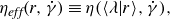 \begin{equation} \eta _{\textit{eff}}(r,\dot \gamma )\equiv \eta (\langle \lambda | r\rangle ,\dot \gamma ), \end{equation}
where
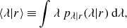 \begin{equation} \langle \lambda |r\rangle \equiv \int \lambda \,p_{\lambda |r}(\lambda |r)\,{\rm d}\lambda , \end{equation}
and $p_{\lambda |r}(\lambda |r)$
is the conditional probability of
$p_{\lambda |r}(\lambda |r)$
is the conditional probability of $\lambda$
occurring at radial position
$\lambda$
occurring at radial position $r$
. This viscosity model (5.3) effectively assumes that the variation in
$r$
. This viscosity model (5.3) effectively assumes that the variation in $\lambda$
about its conditionally average has minimal impact on the flow, which shall be tested in due course. Discretise the
$\lambda$
about its conditionally average has minimal impact on the flow, which shall be tested in due course. Discretise the $s$
-domain as
$s$
-domain as $s_n=n\Delta s$
, with
$s_n=n\Delta s$
, with $\Delta s\ll \tau _{\dot \gamma }$
, the functional (5.2) can be expressed as
$\Delta s\ll \tau _{\dot \gamma }$
, the functional (5.2) can be expressed as
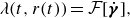 \begin{equation} \lambda (t,r(t))=\mathcal{F}[\dot {\boldsymbol \gamma }], \end{equation}
where $\dot {\boldsymbol \gamma }$
is the vector
$\dot {\boldsymbol \gamma }$
is the vector $\dot {\boldsymbol \gamma }\equiv (\dot \gamma _0, \dot \gamma _1,\dots ,\dot \gamma _q)$
of Lagrangian shear rates
$\dot {\boldsymbol \gamma }\equiv (\dot \gamma _0, \dot \gamma _1,\dots ,\dot \gamma _q)$
of Lagrangian shear rates $\dot \gamma _n\equiv \dot \gamma (t-n\Delta s;\textbf{X},t_0)$
. As
$\dot \gamma _n\equiv \dot \gamma (t-n\Delta s;\textbf{X},t_0)$
. As $G(t-s)\sim \exp (-\Lambda s)$
, if
$G(t-s)\sim \exp (-\Lambda s)$
, if $q\gg 1/(\Delta s\Lambda )$
then the shear history for
$q\gg 1/(\Delta s\Lambda )$
then the shear history for $s\gt q\Delta s$
has no impact on
$s\gt q\Delta s$
has no impact on $\lambda (t,r(t))$
. Similarly, the discrete Lagrangian radial history can be encoded as
$\lambda (t,r(t))$
. Similarly, the discrete Lagrangian radial history can be encoded as $\textbf{r}=\{r_0,r_1,\dots ,r_q\}$
, where
$\textbf{r}=\{r_0,r_1,\dots ,r_q\}$
, where $r_n\equiv r(t-n\Delta s)$
for
$r_n\equiv r(t-n\Delta s)$
for $n=0:q$
.
$n=0:q$
.
From (5.2), the conditional average (5.4) can be conceptualised as a path integral (Kleinert Reference Kleinert2006; Wio Reference Wio2013) of $\mathcal{F}$
over all the shear
$\mathcal{F}$
over all the shear $\dot {\boldsymbol \gamma }$
and radial
$\dot {\boldsymbol \gamma }$
and radial $\textbf{r}$
histories backwards in time from a particle at position
$\textbf{r}$
histories backwards in time from a particle at position $r(t)$
at current time
$r(t)$
at current time $t$
to
$t$
to $r(t-q\Delta s)$
at time
$r(t-q\Delta s)$
at time $t-q\Delta s$
as
$t-q\Delta s$
as
 \begin{equation} \langle \lambda |r\rangle =\int _{\textbf{r}}\int _{\dot {\boldsymbol \gamma }}\mathcal{F}[\dot {\boldsymbol \gamma }]\mathcal{P}[\dot {\boldsymbol \gamma },\textbf{r}|r_0=r]d^q\dot {\boldsymbol \gamma }d^q\textbf{r}, \end{equation}
where $\mathcal{P}[\dot {\boldsymbol \gamma },\textbf{r}|r_0=r]$
is the conditional probability of the shear history
$\mathcal{P}[\dot {\boldsymbol \gamma },\textbf{r}|r_0=r]$
is the conditional probability of the shear history $\dot {\boldsymbol \gamma }$
and radial history
$\dot {\boldsymbol \gamma }$
and radial history $\textbf{r}$
given current radial position
$\textbf{r}$
given current radial position $r$
. This general formalism describes evolution of the structural parameter over a broad range of thixotropic and rheological models.
$r$
. This general formalism describes evolution of the structural parameter over a broad range of thixotropic and rheological models.
Via Bayes’ theorem, the conditional probability $\mathcal{P}[\dot {\boldsymbol \gamma },\textbf{r}|r_0=r]$
is related to the joint probability
$\mathcal{P}[\dot {\boldsymbol \gamma },\textbf{r}|r_0=r]$
is related to the joint probability $\mathcal{P}[\dot {\boldsymbol \gamma },\textbf{r}]$
of shear rate history
$\mathcal{P}[\dot {\boldsymbol \gamma },\textbf{r}]$
of shear rate history $\dot {\boldsymbol \gamma }$
and radial history as
$\dot {\boldsymbol \gamma }$
and radial history as
 \begin{equation} \mathcal{P}[\dot {\boldsymbol \gamma },\textbf{r}]=\mathcal{P}[\dot {\boldsymbol \gamma }|r]\mathcal{P}[\textbf{r}|r_0=r], \end{equation}
where $\mathcal{P}[\textbf{r}|r_0=r]$
is the conditional probability of
$\mathcal{P}[\textbf{r}|r_0=r]$
is the conditional probability of $\textbf{r}$
given
$\textbf{r}$
given $r_0=r$
. Under the assumption that the shear rate and radial position evolve in a Markovian manner in time, the joint probability
$r_0=r$
. Under the assumption that the shear rate and radial position evolve in a Markovian manner in time, the joint probability $\mathcal{P}[\dot {\boldsymbol \gamma },\textbf{r}]$
can then be expanded as
$\mathcal{P}[\dot {\boldsymbol \gamma },\textbf{r}]$
can then be expanded as
 \begin{align} \mathcal{P}[\dot {\boldsymbol \gamma },\textbf{r}]&=\mathcal{P}[\{\dot \gamma _0,r_0\},\{\dot \gamma _1,r_1\},\dots ,\{\dot \gamma _q,r_q\}]\nonumber \\ &=P_{\Delta s}(\dot \gamma _{q},r_{q}|\dot \gamma _{q-1},r_{q-1})\dots P_{\Delta s}(\dot \gamma _2,r_2|\dot \gamma _1,r_1)P_{\Delta s}(\dot \gamma _1,r_1|\dot \gamma _0,r_0)p_{\dot \gamma ,r}(\dot \gamma _0,r_0), \end{align}
where the backwards propagator $P_{\Delta s}(\dot \gamma _{n+1},r_{n+1} | \dot \gamma _{n},r_{n})$
is the conditional probability of a material element being at position
$P_{\Delta s}(\dot \gamma _{n+1},r_{n+1} | \dot \gamma _{n},r_{n})$
is the conditional probability of a material element being at position $r_{n+1}$
with shear rate
$r_{n+1}$
with shear rate $\dot \gamma _{n+1}$
at time
$\dot \gamma _{n+1}$
at time $t-(n+1)\Delta s$
given it is at position
$t-(n+1)\Delta s$
given it is at position $r_{n}$
with shear rate
$r_{n}$
with shear rate $\dot \gamma _{n}$
at time
$\dot \gamma _{n}$
at time $t-n\Delta s$
. Using the Chapman–Kolmogorov equation for Markov processes
$t-n\Delta s$
. Using the Chapman–Kolmogorov equation for Markov processes
 \begin{equation} P_{2\Delta s}(\dot \gamma _n,r_n|\dot \gamma _{n+2},r_{n+2})=\!\!\int _{-\infty }^\infty \!\int _{-\infty }^\infty \!\!\!P(\dot \gamma _n,r_n|\dot \gamma _{n+2},r_{n+2})P(\dot \gamma _n,r_n|\dot \gamma _{n+2},r_{n+2}){\rm d}\dot \gamma _{n+1}{\rm d}r_{n+1}\!, \end{equation}
the path integral (5.6) can then be expressed explicitly as
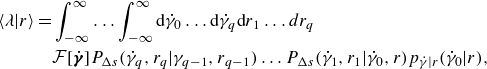 \begin{align} \langle \lambda | r\rangle &=\int _{-\infty }^\infty \dots \int _{-\infty }^\infty {\rm d}\dot {\gamma }_0\dots {\rm d}\dot {\gamma }_q {\rm d}r_1\dots dr_q \nonumber \\ &\quad \mathcal{F}[\dot {\boldsymbol \gamma }] P_{\Delta s}(\dot \gamma _{q},r_{q}|\gamma _{q-1},r_{q-1})\dots P_{\Delta s}(\dot \gamma _1,r_1 | \dot \gamma _0,r)p_{\dot \gamma |r}(\dot \gamma _0|r), \end{align}
where $p_{\dot \gamma |r}(\dot \gamma |r)$
is the conditional probability of
$p_{\dot \gamma |r}(\dot \gamma |r)$
is the conditional probability of $\dot \gamma$
given
$\dot \gamma$
given $r$
. Hence, the conditionally averaged structural parameter
$r$
. Hence, the conditionally averaged structural parameter $\langle \lambda | r\rangle$
is dependent upon the thixotropic functional
$\langle \lambda | r\rangle$
is dependent upon the thixotropic functional $\mathcal{F}$
and the stochastic process for
$\mathcal{F}$
and the stochastic process for $\dot \gamma (t,r(t))$
and
$\dot \gamma (t,r(t))$
and $r(t)$
via the backwards propagator
$r(t)$
via the backwards propagator $P_{\Delta s}$
. Typically, path integrals such as (5.10) are notoriously difficult to solve for all but simple linear systems (Kleinert Reference Kleinert2006), however, in § 5.3 we show that significant simplifications to (5.6) arise for the simple stochastic models for shear and radial history that are developed as follows.
$P_{\Delta s}$
. Typically, path integrals such as (5.10) are notoriously difficult to solve for all but simple linear systems (Kleinert Reference Kleinert2006), however, in § 5.3 we show that significant simplifications to (5.6) arise for the simple stochastic models for shear and radial history that are developed as follows.
5.2. Stochastic models for radial position and shear rate history
In order to solve the path integral (5.10), we require stochastic models for Lagrangian shear rate and radial position. Although there exist more sophisticated models for radial transport in turbulent pipe flow (Bocksell & Loth Reference Bocksell and Loth2006; Mofakham & Ahmadi Reference Mofakham and Ahmadi2019), we seek a simple model that yields analytic closure of (5.10). Following Dentz, Kang & Borgne (Reference Dentz, Kang and Le Borgne2015), a suitable model for $r(t)$
is developed as follows. In cylindrical coordinates, the advection–dispersion equation for the concentration
$r(t)$
is developed as follows. In cylindrical coordinates, the advection–dispersion equation for the concentration $c(r,t)$
of an ensemble of passive tracer particles is given by the advection–dispersion equation
$c(r,t)$
of an ensemble of passive tracer particles is given by the advection–dispersion equation
 \begin{equation} \frac {\partial c(r,t)}{\partial t} +\frac {1}{r}\frac {\partial }{\partial r}\left [r \bar {v}_r(r) c(r,t)\right ] -\frac {1}{r}\frac {\partial }{\partial r}\left (r D_r(r)\frac {\partial c}{\partial r}\right )=0,\quad \frac {\partial c}{\partial r}\Big |_{r=0}=\frac {\partial c}{\partial r}\Big |_{r=1}=0, \end{equation}
where $\bar {v}_r(r)$
and
$\bar {v}_r(r)$
and $D_r(r)$
, respectively, are the Lagrangian radial mean transport velocity and dispersion coefficient. Here
$D_r(r)$
, respectively, are the Lagrangian radial mean transport velocity and dispersion coefficient. Here $\bar {v}_r(r)\equiv \langle v_r(\textbf{x}(t;\textbf{X},t_0),t)\rangle =0$
and
$\bar {v}_r(r)\equiv \langle v_r(\textbf{x}(t;\textbf{X},t_0),t)\rangle =0$
and $D_r(r)$
is related to the Lagrangian radial velocity fluctuations
$D_r(r)$
is related to the Lagrangian radial velocity fluctuations $v'_r(\textbf{x}(t;\textbf{X},t_0),t)\equiv v_r(\textbf{x}(t;\textbf{X},t_0),t)-\bar {v}_r(r)$
via the fluctuation–dissipation theorem as
$v'_r(\textbf{x}(t;\textbf{X},t_0),t)\equiv v_r(\textbf{x}(t;\textbf{X},t_0),t)-\bar {v}_r(r)$
via the fluctuation–dissipation theorem as
 \begin{equation} D_r(r)=\int _0^\infty \langle v_r^\prime (\textbf{x}(t;\textbf{X},t_0),t)v_r^\prime (\textbf{x}(t+\tau ;\textbf{X},t_0),t+\tau )\rangle {\rm d}\tau , \end{equation}
where the angled brackets denotes an average over all times $t$
, azimuthal
$t$
, azimuthal $\theta$
and axial
$\theta$
and axial $z$
coordinates. For any well-behaved
$z$
coordinates. For any well-behaved $D_r(r)$
, in the long-time limit
$D_r(r)$
, in the long-time limit $t\rightarrow \infty$
the particle concentration approaches the homogeneous state
$t\rightarrow \infty$
the particle concentration approaches the homogeneous state $c(r,t)\rightarrow c_0$
. The particle concentration
$c(r,t)\rightarrow c_0$
. The particle concentration $c(r,t)$
is related to the probability
$c(r,t)$
is related to the probability $p_r(r,t)$
of finding a tracer particle at position
$p_r(r,t)$
of finding a tracer particle at position $r$
at time
$r$
at time $t$
as
$t$
as
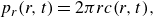 \begin{equation} p_r(r,t)=2\pi r c(r,t), \end{equation}
and so this probability is governed by the radial Fokker–Planck equation
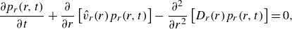 \begin{align} \frac {\partial p_r(r,t)}{\partial t}+\frac {\partial }{\partial r}\left [\hat {v}_r(r)p_r(r,t)\right ]-\frac {\partial ^2}{\partial r^2}\left [D_r(r)p_r(r,t)\right ]=0, \end{align}
with insulating boundary conditions
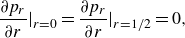 \begin{equation} \frac {\partial p_r}{\partial r}\Big |_{r=0}=\frac {\partial p_r}{\partial r}\Big |_{r=1/2}=0, \end{equation}
and
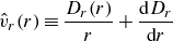 \begin{equation} \hat {v}_r(r)\equiv \frac {D_r(r)}{r}+\frac {{\rm d}D_r}{{\rm d}r} \end{equation}
is the effective radial velocity due to the radial dispersivity $D_r(r)$
. In the long-time limit
$D_r(r)$
. In the long-time limit $t\rightarrow \infty$
, the particle probability in (5.14) approaches the equilibrium distribution
$t\rightarrow \infty$
, the particle probability in (5.14) approaches the equilibrium distribution $p_r(r)=8r$
. Following the Itô interpretation of a stochastic process, the equivalent Langevin equation for the radial position
$p_r(r)=8r$
. Following the Itô interpretation of a stochastic process, the equivalent Langevin equation for the radial position $r(t)$
of a single tracer particle with
$r(t)$
of a single tracer particle with $p_r(r,t)=\langle \delta (r-r(t))\rangle$
is then
$p_r(r,t)=\langle \delta (r-r(t))\rangle$
is then
 \begin{equation} \frac {{\rm d}r(t)}{{\rm d}t}=\hat {v}_r[r(t)]+\sqrt {2D(r(t))}\xi _r(t),\quad r(t)\in [0,1/2], \end{equation}
where $\xi _r(t)$
is a Gaussian white noise with zero mean and unit variance which is delta correlated in time;
$\xi _r(t)$
is a Gaussian white noise with zero mean and unit variance which is delta correlated in time; $\langle \xi _r(t)\xi _r(t^\prime )\rangle =\delta (t-t^\prime )$
.
$\langle \xi _r(t)\xi _r(t^\prime )\rangle =\delta (t-t^\prime )$
.
The above formulation makes several assumptions regarding the radial position and radial velocity processes. First, it is assumed that the Lagrangian radial velocity fluctuation $v_r^\prime (\textbf{x}(t;\textbf{X},t_0),t)$
is a stochastic Markov process in that it decorrelates on a time scale
$v_r^\prime (\textbf{x}(t;\textbf{X},t_0),t)$
is a stochastic Markov process in that it decorrelates on a time scale $\tau _v$
that is much faster than the radial position decorrelation time
$\tau _v$
that is much faster than the radial position decorrelation time $\tau _r$
, i.e.
$\tau _r$
, i.e. $\tau _v\ll \tau _r$
, which validates the assumption of delta-correlated Gaussian noise
$\tau _v\ll \tau _r$
, which validates the assumption of delta-correlated Gaussian noise $\xi _r(t)$
in (5.17). The other assumption is that the decorrelation processes for radial velocity and position are radially independent. These assumptions are tested as follows.
$\xi _r(t)$
in (5.17). The other assumption is that the decorrelation processes for radial velocity and position are radially independent. These assumptions are tested as follows.
Figure 14(a) shows the normalised Lagrangian autocorrelation functions for the radial velocity ( $R_{v_r'v_r'}$
), radial position (
$R_{v_r'v_r'}$
), radial position ( $R_{r'r'}$
) and shear rate (
$R_{r'r'}$
) and shear rate ( $R_{\dot \gamma '\dot \gamma '}$
) fluctuations from the DNS simulations for
$R_{\dot \gamma '\dot \gamma '}$
) fluctuations from the DNS simulations for $\Lambda =1$
as
$\Lambda =1$
as
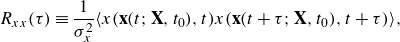 \begin{align} R_{xx}(\tau )&\equiv \frac {1}{\sigma ^2_{x}}\langle x(\textbf{x}(t;\textbf{X},t_0),t)x(\textbf{x}(t+\tau ;\textbf{X},t_0),t+\tau )\rangle , \end{align}
with $x=v_r'$
,
$x=v_r'$
, $x=r'$
,
$x=r'$
, $x=\dot \gamma '$
. From this data, the decorrelation times for the radial velocity, radial position and shear rate are computed as
$x=\dot \gamma '$
. From this data, the decorrelation times for the radial velocity, radial position and shear rate are computed as $\tau _v\approx 0.57$
,
$\tau _v\approx 0.57$
, $\tau _r\approx 6.30$
,
$\tau _r\approx 6.30$
, $\tau _{\dot \gamma }\approx 4.86$
. Hence, the assumption that
$\tau _{\dot \gamma }\approx 4.86$
. Hence, the assumption that $\tau _v\ll \tau _r$
is approximately true but not strictly valid. Under the assumption that the radial velocity fluctuation follows a Markov process with the exponentially decaying autocorrelation function
$\tau _v\ll \tau _r$
is approximately true but not strictly valid. Under the assumption that the radial velocity fluctuation follows a Markov process with the exponentially decaying autocorrelation function
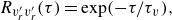 \begin{equation} R_{v_r^\prime v_r^\prime }(\tau )=\exp (-\tau /\tau _v), \end{equation}
the radial dispersivity $D_r(r)$
in (5.12) is
$D_r(r)$
in (5.12) is
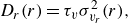 \begin{equation} D_r(r)=\tau _v\sigma ^2_{v_r}(r), \end{equation}
where $\sigma ^2_{v_r}(r)$
is the conditional variance
$\sigma ^2_{v_r}(r)$
is the conditional variance $\sigma ^2_{v_r}(r)=\langle v_r^\prime (\textbf{x}|_{r},t)v_r^\prime (\textbf{x}|_{r},t)\rangle$
. To compare results of the stochastic model with the DNS solutions (which include finite diffusivity of
$\sigma ^2_{v_r}(r)=\langle v_r^\prime (\textbf{x}|_{r},t)v_r^\prime (\textbf{x}|_{r},t)\rangle$
. To compare results of the stochastic model with the DNS solutions (which include finite diffusivity of $\lambda$
for numerical stability), the scalar diffusivity
$\lambda$
for numerical stability), the scalar diffusivity $1/Pe=10^{-3}$
is also added to (5.20). However, we note for many complex fluids such as suspensions and emulsions,
$1/Pe=10^{-3}$
is also added to (5.20). However, we note for many complex fluids such as suspensions and emulsions, $1/Pe$
is negligibly small and so can be neglected. The resultant radial dispersivity is shown in figure 14(b), indicating that as expected, dispersion is moderate in the pipe core, reaches a maximum in the buffer layer before decaying to the scalar diffusivity
$1/Pe$
is negligibly small and so can be neglected. The resultant radial dispersivity is shown in figure 14(b), indicating that as expected, dispersion is moderate in the pipe core, reaches a maximum in the buffer layer before decaying to the scalar diffusivity $\alpha$
at the pipe wall. Application of this radial dispersivity to the random walk model (5.17) yields the mean square displacement data shown in figure 15(a), which agrees well with the DNS results for
$\alpha$
at the pipe wall. Application of this radial dispersivity to the random walk model (5.17) yields the mean square displacement data shown in figure 15(a), which agrees well with the DNS results for $\Lambda =1$
, and provides a close match to the radial position decorrelation curve shown in figure 14(a).
$\Lambda =1$
, and provides a close match to the radial position decorrelation curve shown in figure 14(a).
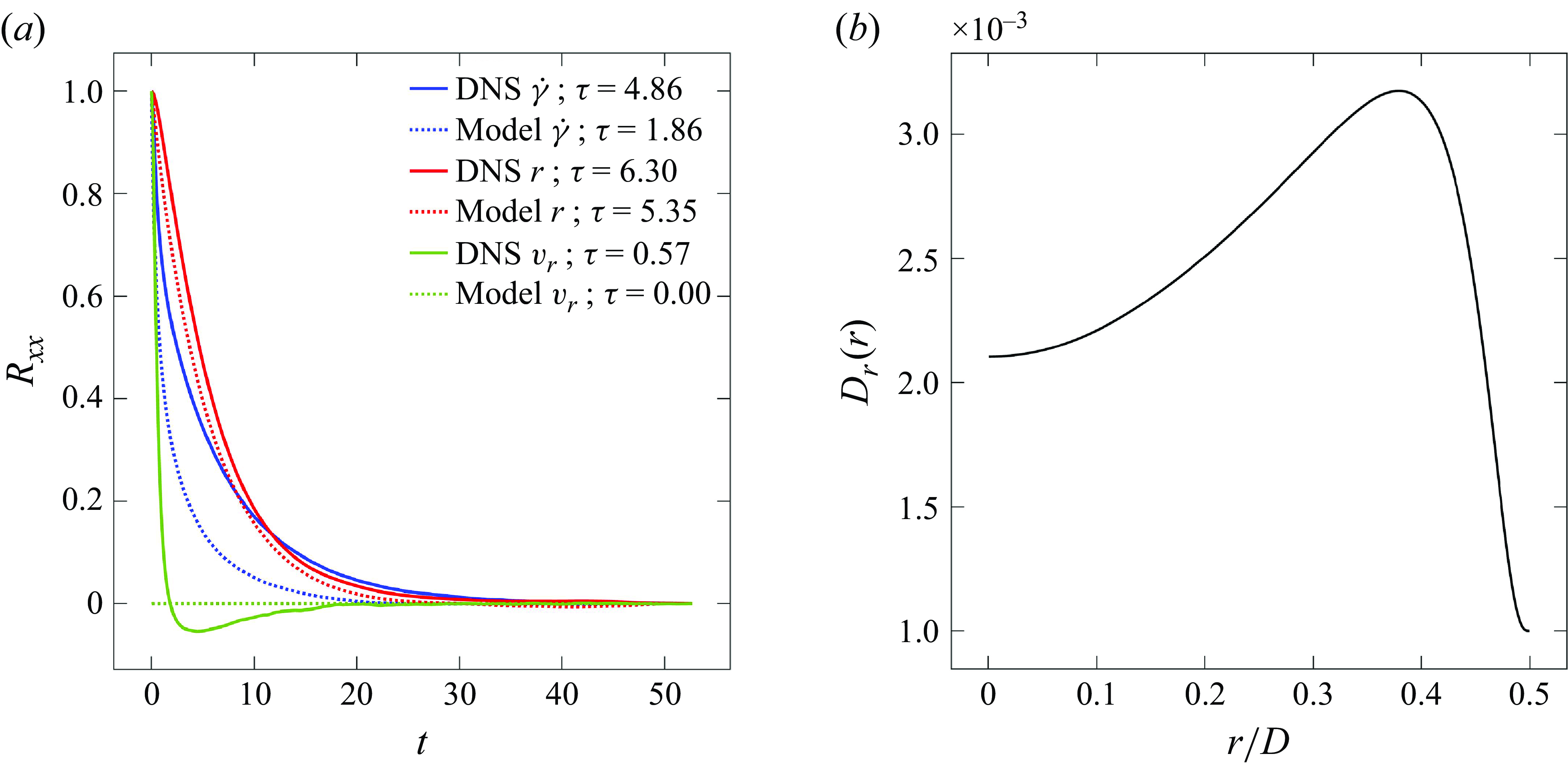
Figure 14. (a) Comparison of Lagrangian autocorrelation functions $R_{xx}$
for radial velocity fluctuation
$R_{xx}$
for radial velocity fluctuation $x=v_r'$
, radial position
$x=v_r'$
, radial position $x=r'$
and shear rate
$x=r'$
and shear rate $x=\dot \gamma '$
for thixotropic flows with
$x=\dot \gamma '$
for thixotropic flows with $\Lambda =1$
, from (solid lines) DNS results and (dotted lines) the stochastic model (5.17). (b) Radial dispersivity
$\Lambda =1$
, from (solid lines) DNS results and (dotted lines) the stochastic model (5.17). (b) Radial dispersivity $D_r(r)$
from the DNS computations of the case
$D_r(r)$
from the DNS computations of the case $\Lambda =1$
.
$\Lambda =1$
.
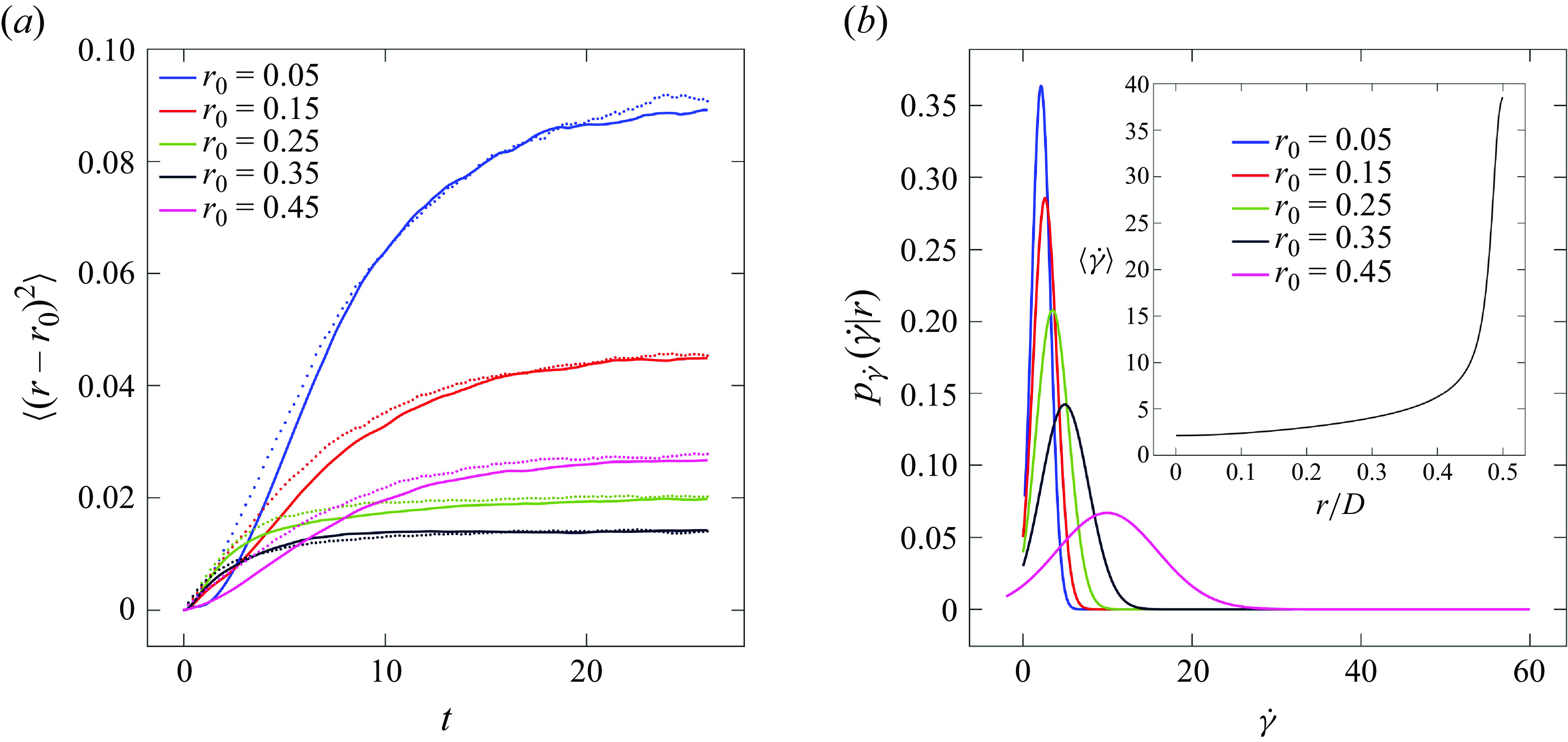
Figure 15. (a) Comparison of mean square displacement $\langle (r-r_0)^2\rangle$
along typical particle trajectories for thixotropic flows with
$\langle (r-r_0)^2\rangle$
along typical particle trajectories for thixotropic flows with $\Lambda =1$
, from (solid lines) DNS results and (dotted lines) the stochastic model (5.17). (b) Conditional p.d.f. of shear rate at various radial locations
$\Lambda =1$
, from (solid lines) DNS results and (dotted lines) the stochastic model (5.17). (b) Conditional p.d.f. of shear rate at various radial locations $p_{\dot \gamma |r}(\dot \gamma |r)$
from the DNS computations of the case
$p_{\dot \gamma |r}(\dot \gamma |r)$
from the DNS computations of the case $\Lambda =1$
. Inset: distribution of conditionally averaged shear rate
$\Lambda =1$
. Inset: distribution of conditionally averaged shear rate $\langle \dot \gamma |r\rangle$
from the DNS computations of
$\langle \dot \gamma |r\rangle$
from the DNS computations of $\Lambda =1$
.
$\Lambda =1$
.
As shown in figure 14(a), the Lagrangian shear rate and radial position fluctuations appear to decorrelate on similar time scales $\tau _{\dot \gamma }\sim \tau _r$
, suggesting that shear rate fluctuations are dominated by fluctuations in radial position rather than temporal fluctuations at fixed radial position. As such, we propose a very simple deterministic relationship between the Lagrangian shear rate
$\tau _{\dot \gamma }\sim \tau _r$
, suggesting that shear rate fluctuations are dominated by fluctuations in radial position rather than temporal fluctuations at fixed radial position. As such, we propose a very simple deterministic relationship between the Lagrangian shear rate $\dot \gamma (t,r(t))$
and radial position based on the conditional mean as
$\dot \gamma (t,r(t))$
and radial position based on the conditional mean as
 \begin{equation} \dot \gamma (t,r(t))\equiv \dot \gamma (t,\textbf{X};t_0)\approx \langle \dot \gamma |r(t)\rangle , \end{equation}
hence all fluctuations in Lagrangian shear rate are driven by fluctuations in radial position. The conditional shear rate p.d.f. is shown in figure 15(b), indicating that the shear rate is fairly peaked in the pipe bulk but broadens near the wall, and the inset of this figure shows that the average shear rate monotonically decreases from the pipe bulk to the wall. Figure 14(a) indicates that this stochastic model yields a significantly faster decorrelation rate ( $\tau _{\dot \gamma }=1.86$
) than that observed in the DNS simulations (
$\tau _{\dot \gamma }=1.86$
) than that observed in the DNS simulations ( $\tau _{\dot \gamma }=4.86$
), which may be attributed to approximating the p.d.f.s in figure 15(b) with delta functions. Although approximate, this stochastic model for Lagrangian shear rate history closes the path integral (5.10).
$\tau _{\dot \gamma }=4.86$
), which may be attributed to approximating the p.d.f.s in figure 15(b) with delta functions. Although approximate, this stochastic model for Lagrangian shear rate history closes the path integral (5.10).
From (5.10), the conditional average $\langle \lambda |r\rangle$
involves an ensemble average over all trajectories that arrive at position
$\langle \lambda |r\rangle$
involves an ensemble average over all trajectories that arrive at position $r$
at current time
$r$
at current time $t$
. Hence, we consider the adjoint problem that describes the evolution of Lagrangian radial position or tracer particles that are currently at position
$t$
. Hence, we consider the adjoint problem that describes the evolution of Lagrangian radial position or tracer particles that are currently at position $r$
at time
$r$
at time $t$
backwards in time. If we write the radial position probability as the probability of tracer particle being at position
$t$
backwards in time. If we write the radial position probability as the probability of tracer particle being at position $r$
at time
$r$
at time $t$
given it as originally at position
$t$
given it as originally at position $r_0$
at time
$r_0$
at time $t-s\lt t$
as
$t-s\lt t$
as $p_r(r,t)=p_r(r,t|r_s,t-s)$
, then the backward Fokker–Planck equation is given by the adjoint of (5.14) as
$p_r(r,t)=p_r(r,t|r_s,t-s)$
, then the backward Fokker–Planck equation is given by the adjoint of (5.14) as
 \begin{equation} \frac {\partial p_r(r,t|r_s,t-s)}{\partial s}-\hat {v}_r(r_s)\frac {\partial }{\partial r_s}p_r(r,t|r_s,t-s)-D_r(r_s)\frac {\partial ^2}{\partial r_s^2}p_r(r,t|r_s,t-s)=0, \end{equation}
with insulating boundary conditions (5.15) and initial condition $p_r(r,t|r_0,t)=\delta (r_0-r)$
at
$p_r(r,t|r_0,t)=\delta (r_0-r)$
at $s=0$
. Using (5.21) and (5.22), the path integral (5.10) then simplifies to
$s=0$
. Using (5.21) and (5.22), the path integral (5.10) then simplifies to
 \begin{equation} \langle \lambda | r\rangle =\int _{-\infty }^\infty \dots \int _{-\infty }^\infty {\rm d}r_1\dots {\rm d}r_q\mathcal{F}[\langle \dot \gamma |\textbf{r}\rangle ] P_{\Delta s}(r_q|r_{q-1})\dots P_{\Delta s}(r_1|,r), \end{equation}
where the backwards propagator for $r$
is given as
$r$
is given as $P_{\Delta s}(r_{n+1}|r_n)\equiv p_r(r,t|r_{\Delta s},t-\Delta s)$
, which is a Green’s function for the backward Fokker–Planck equation.
$P_{\Delta s}(r_{n+1}|r_n)\equiv p_r(r,t|r_{\Delta s},t-\Delta s)$
, which is a Green’s function for the backward Fokker–Planck equation.
5.3. Structural parameter
An expression for the structural parameter is given by discretising (5.1) with respect to $s$
as
$s$
as
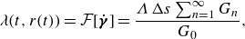 \begin{equation} \lambda (t,r(t))=\mathcal{F}[\dot {\boldsymbol \gamma }]=\frac {\Lambda \,\Delta s\sum _{n=1}^\infty G_n}{G_0}, \end{equation}
where $G_n\equiv G(t-n\Delta s;\textbf{X},t_0)$
is given as
$G_n\equiv G(t-n\Delta s;\textbf{X},t_0)$
is given as
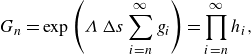 \begin{equation} G_n=\exp \left (\Lambda \,\Delta s\sum _{i=n}^\infty g_i\right )=\prod _{i=n}^\infty h_i, \end{equation}
where $h_n\equiv \exp [\Lambda \,\Delta s(1+K\dot \gamma _n)]\gt 1$
. From these relations, the structural parameter is then
$h_n\equiv \exp [\Lambda \,\Delta s(1+K\dot \gamma _n)]\gt 1$
. From these relations, the structural parameter is then
 \begin{align} \lambda (t,r(t))=\mathcal{F}[\dot {\boldsymbol \gamma }]=\Lambda \,\Delta s\sum _{n=1}^\infty \frac {1}{\prod _{i=0}^n h_i}=&\Lambda \,\Delta s\left (\frac {1}{h_0}+\frac {1}{h_0h_1}+\frac {1}{h_0h_1h_2}+\dots \right ). \end{align}
Hence, the functional $\mathcal{F}[\dot {\boldsymbol \gamma }]$
that governs the structural parameter
$\mathcal{F}[\dot {\boldsymbol \gamma }]$
that governs the structural parameter $\lambda$
depends upon the shear rate history, and convergence of the sum in (5.26) is governed by the thixoviscous number
$\lambda$
depends upon the shear rate history, and convergence of the sum in (5.26) is governed by the thixoviscous number $\Lambda$
. Averaging of (5.26) yields
$\Lambda$
. Averaging of (5.26) yields
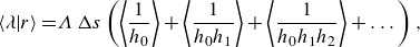 \begin{align} \langle \lambda |r\rangle =&\Lambda \,\Delta s\left (\left \langle \frac {1}{h_0}\right \rangle +\left \langle \frac {1}{h_0h_1}\right \rangle +\left \langle \frac {1}{h_0h_1h_2}\right \rangle +\dots \right ), \end{align}
where evaluation of the ensemble averaged terms $\langle \cdot \rangle$
corresponds to solution of the path integral (5.10). Note that this expression is completely general and not contingent upon the stochastic model developed in § 5.2.
$\langle \cdot \rangle$
corresponds to solution of the path integral (5.10). Note that this expression is completely general and not contingent upon the stochastic model developed in § 5.2.
For this stochastic model, the Lagrangian shear rate $\dot \gamma (t,r(t))$
is given by the conditional average
$\dot \gamma (t,r(t))$
is given by the conditional average $\langle \dot \gamma |r(t)\rangle$
, hence insertion of (5.26) into (5.23) yields
$\langle \dot \gamma |r(t)\rangle$
, hence insertion of (5.26) into (5.23) yields
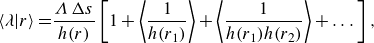 \begin{align} \langle \lambda |r\rangle =&\frac {\Lambda \,\Delta s}{h(r)} \left [1+\left \langle \frac {1}{h(r_1)}\right \rangle +\left \langle \frac {1}{h(r_1)h(r_2)}\right \rangle +\dots \right ], \end{align}
where
 \begin{equation} h(r)\equiv \exp \left (\Lambda \,\Delta s[1+K\langle \dot \gamma |r\rangle ]\right ). \end{equation}
The averages in (5.28) are then given by the backwards Fokker–Planck propagator
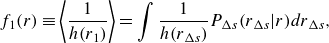 \begin{align} f_1(r)\equiv \left \langle \frac {1}{h(r_1)}\right \rangle &=\int \frac {1}{h(r_{\Delta s})}P_{\Delta s}(r_{\Delta s}|r)dr_{\Delta s}, \end{align}
 \begin{align} f_n(r)\equiv \left \langle \frac {1}{\prod _{i=1}^n h(r_i)}\right \rangle &=\int \frac {1}{h(r_{\Delta s})}P_{\Delta s}(r_{\Delta s}|r)f_{n-1}(r_{\Delta s}){\rm d}r_{\Delta s}, \end{align}
and so
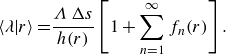 \begin{align} \langle \lambda |r\rangle =&\frac {\Lambda \,\Delta s}{h(r)} \left [1+\sum _{n=1}^\infty f_n(r)\right ]. \end{align}
Note that the length of the relevant shear history depends strongly upon the thixoviscous parameter $\Lambda$
.
$\Lambda$
.
In the limit of fast kinetics with $\Lambda \gg 1$
, we set
$\Lambda \gg 1$
, we set $\Delta s\lll 1$
very small such that
$\Delta s\lll 1$
very small such that $\Lambda \,\Delta s\ll 1$
and so for
$\Lambda \,\Delta s\ll 1$
and so for $s=n\Delta s$
,
$s=n\Delta s$
, $n=0:q$
the radial position
$n=0:q$
the radial position $r(t-s)$
is still centred about
$r(t-s)$
is still centred about $r(t)$
, hence
$r(t)$
, hence
 \begin{align} f_n(r)=\int \frac {1}{h(r_{\Delta s})}\delta (r-r_{\Delta s})f_{n-1}(r_{\Delta s}){\rm d}r_{\Delta s}=\frac {1}{h(r)}f_{n-1}(r_{\Delta s})=\frac {1}{h(r)^n}, \end{align}
and so we recover the conditionally averaged shear rate analogue to the shear thinning viscosity (4.12) as
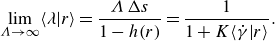 \begin{equation} \lim _{\Lambda \rightarrow \infty }\langle \lambda |r\rangle = \frac {\Lambda \,\Delta s}{1-h(r)}=\frac {1}{1+K\langle \dot \gamma |r\rangle }. \end{equation}
Note that if we relax the assumption (5.21), a similar derivation based on (5.27) exactly recovers the shear thinning viscosity (4.12). In the slow kinetics regime, the terms in (5.32) converge very slowly as $\Lambda \ll 1$
and the conditional probability converges to
$\Lambda \ll 1$
and the conditional probability converges to
 \begin{equation} \lim _{s\rightarrow \infty }p_r(r,t|r_s,t-s)=p_{r}(r)=8r, \end{equation}
then for $\Lambda \,\Delta s\ll 1$
, the ensemble averages are
$\Lambda \,\Delta s\ll 1$
, the ensemble averages are
 \begin{equation} f_n=\int \frac {1}{h(r_{\Delta s})}p_{r}(r_{\Delta s})\, f_{n-1}\,dr_{\Delta s}=[1-\Lambda \,\Delta s(1+K\langle \dot \gamma \rangle )]f_{n-1}, \end{equation}
and so
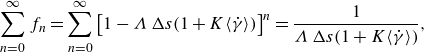 \begin{equation} \sum _{n=0}^\infty f_n=\sum _{n=0}^\infty \left [1-\Lambda \,\Delta s(1+K\langle \dot \gamma \rangle )\right ]^n=\frac {1}{\Lambda \,\Delta s(1+K\langle \dot \gamma \rangle )}, \end{equation}
and so we recover the Newtonian viscosity (4.19) as
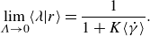 \begin{equation} \lim _{\Lambda \rightarrow 0}\langle \lambda |r\rangle =\frac {1}{1+K\langle \dot \gamma \rangle }. \end{equation}
Hence, the stochastic model for the structural parameter can be applied to the entire range of thixoviscous numbers $\Lambda \in (0,\infty ^+)$
, and recovers the limiting viscosity models for fast and slow kinetics derived in § 4. As such, the effective viscosity for the entire spectrum of the thixotropic kinetic parameter
$\Lambda \in (0,\infty ^+)$
, and recovers the limiting viscosity models for fast and slow kinetics derived in § 4. As such, the effective viscosity for the entire spectrum of the thixotropic kinetic parameter $\Lambda \in (0,\infty ^+)$
is given by the radially dependent viscosity
$\Lambda \in (0,\infty ^+)$
is given by the radially dependent viscosity
 \begin{equation} \eta _{\textit{eff}}(r,\dot \gamma )=\eta (\langle \lambda |r\rangle ,\dot \gamma )=\mu _\infty +(\mu _0-\mu _\infty )\langle \lambda |r\rangle , \end{equation}
the accuracy of which shall be tested as follows.
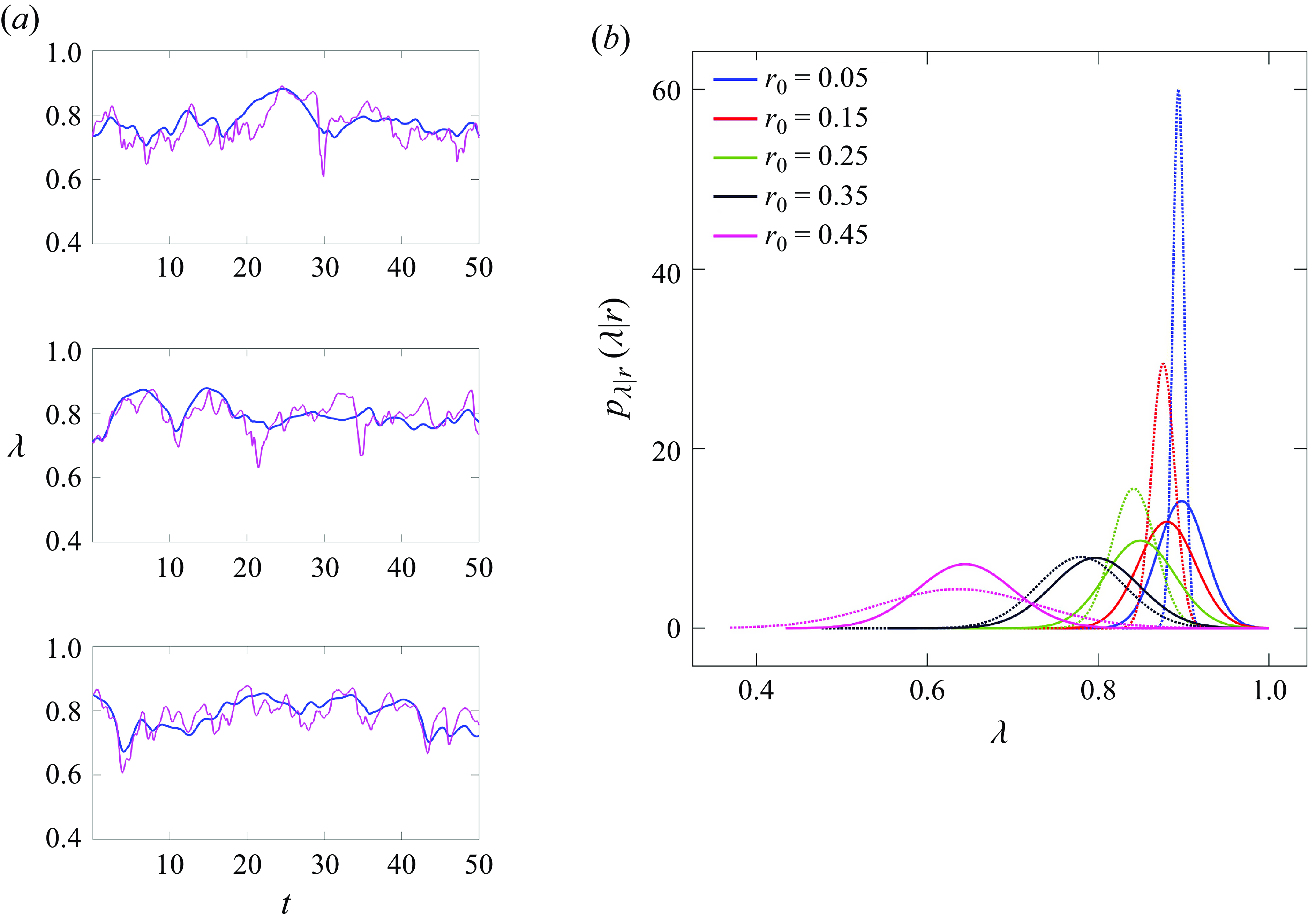
Figure 16. (a) Comparison of structural parameter $\lambda (t;\textbf{X},t_0)$
along representative particle trajectories at
$\lambda (t;\textbf{X},t_0)$
along representative particle trajectories at $r\sim 0.4$
(near the pipe walls) for thixotropic flows with
$r\sim 0.4$
(near the pipe walls) for thixotropic flows with $\Lambda =1$
, from (
$\Lambda =1$
, from (
![]() ) DNS results and (
) DNS results and (
![]() ) solution of Lagrangian equation (4.2) with
) solution of Lagrangian equation (4.2) with $\langle \dot \gamma |r(t)\rangle$
. (b) Comparison of conditional p.d.f. of structural parameter
$\langle \dot \gamma |r(t)\rangle$
. (b) Comparison of conditional p.d.f. of structural parameter $p_\lambda (\lambda |r)$
along typical particle trajectories for thixotropic flows with
$p_\lambda (\lambda |r)$
along typical particle trajectories for thixotropic flows with $\Lambda =1$
, from (solid lines) DNS results and (dotted lines) the stochastic model (5.17).
$\Lambda =1$
, from (solid lines) DNS results and (dotted lines) the stochastic model (5.17).
5.4. Numerical testing of stochastic model
To test the stochastic model developed in the previous section, we compare model predictions for the structural parameter $\langle \lambda |r\rangle$
with DNS computations of
$\langle \lambda |r\rangle$
with DNS computations of $\Lambda =1$
. As the expression (5.32) does not yield closed-form solutions for the averaged structural parameter, we compute
$\Lambda =1$
. As the expression (5.32) does not yield closed-form solutions for the averaged structural parameter, we compute $\langle \lambda |r\rangle$
via random walk simulations of the Langevin equation (5.17), combined with the path integral (5.32). We then test the effective viscosity model
$\langle \lambda |r\rangle$
via random walk simulations of the Langevin equation (5.17), combined with the path integral (5.32). We then test the effective viscosity model $\eta _{\textit{eff}}(r,\dot \gamma )$
by comparing DNS simulations using this model with the full thixotropic model described in § 2.
$\eta _{\textit{eff}}(r,\dot \gamma )$
by comparing DNS simulations using this model with the full thixotropic model described in § 2.
Figure 16(a) shows that for $\Lambda =1$
, the Lagrangian structural parameter computed using Lagrangian shear rate
$\Lambda =1$
, the Lagrangian structural parameter computed using Lagrangian shear rate $\dot \gamma (t;\textbf{X},t_0)$
data (4.2) agrees fairly well with that given directly from the DNS simulations due to the large Damkhöler number (
$\dot \gamma (t;\textbf{X},t_0)$
data (4.2) agrees fairly well with that given directly from the DNS simulations due to the large Damkhöler number ( $Da=10^3$
), as previously discussed in § 4. Conversely, the structural parameter computed via (4.2) using the conditionally averaged shear rate
$Da=10^3$
), as previously discussed in § 4. Conversely, the structural parameter computed via (4.2) using the conditionally averaged shear rate $\langle \dot \gamma |r(t)\rangle$
does not agree as well, but it does shadow the DNS results, indicating that this closure may still accurately predict
$\langle \dot \gamma |r(t)\rangle$
does not agree as well, but it does shadow the DNS results, indicating that this closure may still accurately predict $\langle \lambda |r\rangle$
. Figure 16(b) compares the p.d.f.
$\langle \lambda |r\rangle$
. Figure 16(b) compares the p.d.f. $p_\lambda (\lambda |r)$
for
$p_\lambda (\lambda |r)$
for $\Lambda$
from DNS computations with those given by the stochastic model described in § 5.2. The stochastic model predicts significantly less variance of
$\Lambda$
from DNS computations with those given by the stochastic model described in § 5.2. The stochastic model predicts significantly less variance of $\lambda$
at the core, however, the distributions agree quite well near the pipe wall and the mean
$\lambda$
at the core, however, the distributions agree quite well near the pipe wall and the mean $\lambda$
agrees fairly well throughout, with the relative error in mean as much as 5 %.
$\lambda$
agrees fairly well throughout, with the relative error in mean as much as 5 %.
Figure 17(a) shows that for $\Lambda =1$
, the structural parameter decorrelates slightly faster for the stochastic model than from the DNS simulations, possibly due to the shear model (5.21). Figure 17(b) shows that despite these differences,
$\Lambda =1$
, the structural parameter decorrelates slightly faster for the stochastic model than from the DNS simulations, possibly due to the shear model (5.21). Figure 17(b) shows that despite these differences, $\langle \lambda |r\rangle$
is accurately predicted by the stochastic model when the numerical diffusivity
$\langle \lambda |r\rangle$
is accurately predicted by the stochastic model when the numerical diffusivity $\alpha$
is included in the radial dispersivity
$\alpha$
is included in the radial dispersivity $D_r(r)$
, with relative
$D_r(r)$
, with relative $L_2$
error of 1.86 % . Conversely, exclusion of
$L_2$
error of 1.86 % . Conversely, exclusion of $\alpha$
leads to significant underestimation of
$\alpha$
leads to significant underestimation of $\lambda$
at the pipe wall as
$\lambda$
at the pipe wall as $D_r(r)$
is then zero, leading to trapping of particles for arbitrarily long periods in this high shear region.
$D_r(r)$
is then zero, leading to trapping of particles for arbitrarily long periods in this high shear region.
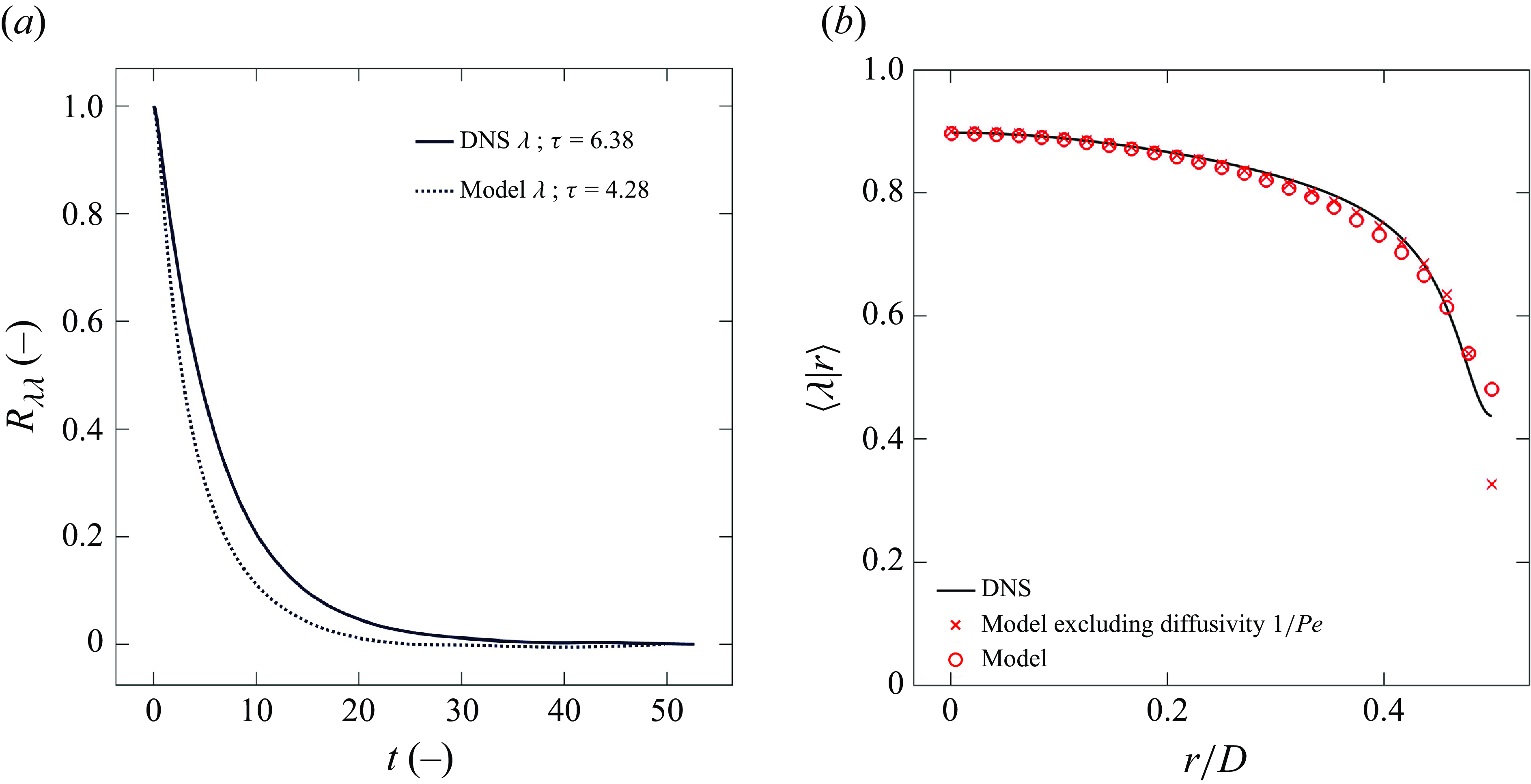
Figure 17. (a) Comparison of Lagrangian autocorrelation functions for structural parameter $R_{\lambda \lambda }$
for thixotropic flows with
$R_{\lambda \lambda }$
for thixotropic flows with $\Lambda =1$
, from (solid lines) DNS results and (dotted lines) the stochastic model (5.17). (b) Comparison of conditionally averaged structural parameter
$\Lambda =1$
, from (solid lines) DNS results and (dotted lines) the stochastic model (5.17). (b) Comparison of conditionally averaged structural parameter $\langle \lambda |r\rangle$
for thixotropic flows with
$\langle \lambda |r\rangle$
for thixotropic flows with $\Lambda =1$
, from (solid lines) DNS results, (
$\Lambda =1$
, from (solid lines) DNS results, (
![]() ) the stochastic model (5.17) and (
) the stochastic model (5.17) and (
![]() ) the stochastic model (5.17) excluding diffusivity
) the stochastic model (5.17) excluding diffusivity $1/Pe$
.
$1/Pe$
.
Figure 18 compares results from DNS computations for $\Lambda = 1$
using the full thixotropic model (2.15), with results from DNS computations using the effective viscosity model (5.39) computed from (i) the stochastic model for
$\Lambda = 1$
using the full thixotropic model (2.15), with results from DNS computations using the effective viscosity model (5.39) computed from (i) the stochastic model for $\langle \lambda |r\rangle$
outlined above, and (ii) direct computation of
$\langle \lambda |r\rangle$
outlined above, and (ii) direct computation of $\langle \lambda |r\rangle$
from DNS results for thixotropic flow. The mean profiles shown in figure 18(a) and 18(b) computed from both the stochastic model and direct calculation of
$\langle \lambda |r\rangle$
from DNS results for thixotropic flow. The mean profiles shown in figure 18(a) and 18(b) computed from both the stochastic model and direct calculation of $\langle \lambda |r\rangle$
show excellent agreement with those obtained using the thixotropic model, with errors in the mean viscosity
$\langle \lambda |r\rangle$
show excellent agreement with those obtained using the thixotropic model, with errors in the mean viscosity $\eta$
(0.84 % and
$\eta$
(0.84 % and $10^{-5}$
%) and axial velocity
$10^{-5}$
%) and axial velocity $U_z$
profiles (1 % and 0.16 %) are low. Figure 18(c–f) also shows that the Reynolds stress profiles (
$U_z$
profiles (1 % and 0.16 %) are low. Figure 18(c–f) also shows that the Reynolds stress profiles ( $u'_{rr},u'_{tt},u'_{zz},u'_{rz}$
) from the DNS results using the stochastic model and from direct computation of
$u'_{rr},u'_{tt},u'_{zz},u'_{rz}$
) from the DNS results using the stochastic model and from direct computation of $\langle \lambda |r\rangle$
both agree very well with the those using the full thixotropic model, with errors as much as 2.4 % and 1.3 %, respectively.
$\langle \lambda |r\rangle$
both agree very well with the those using the full thixotropic model, with errors as much as 2.4 % and 1.3 %, respectively.
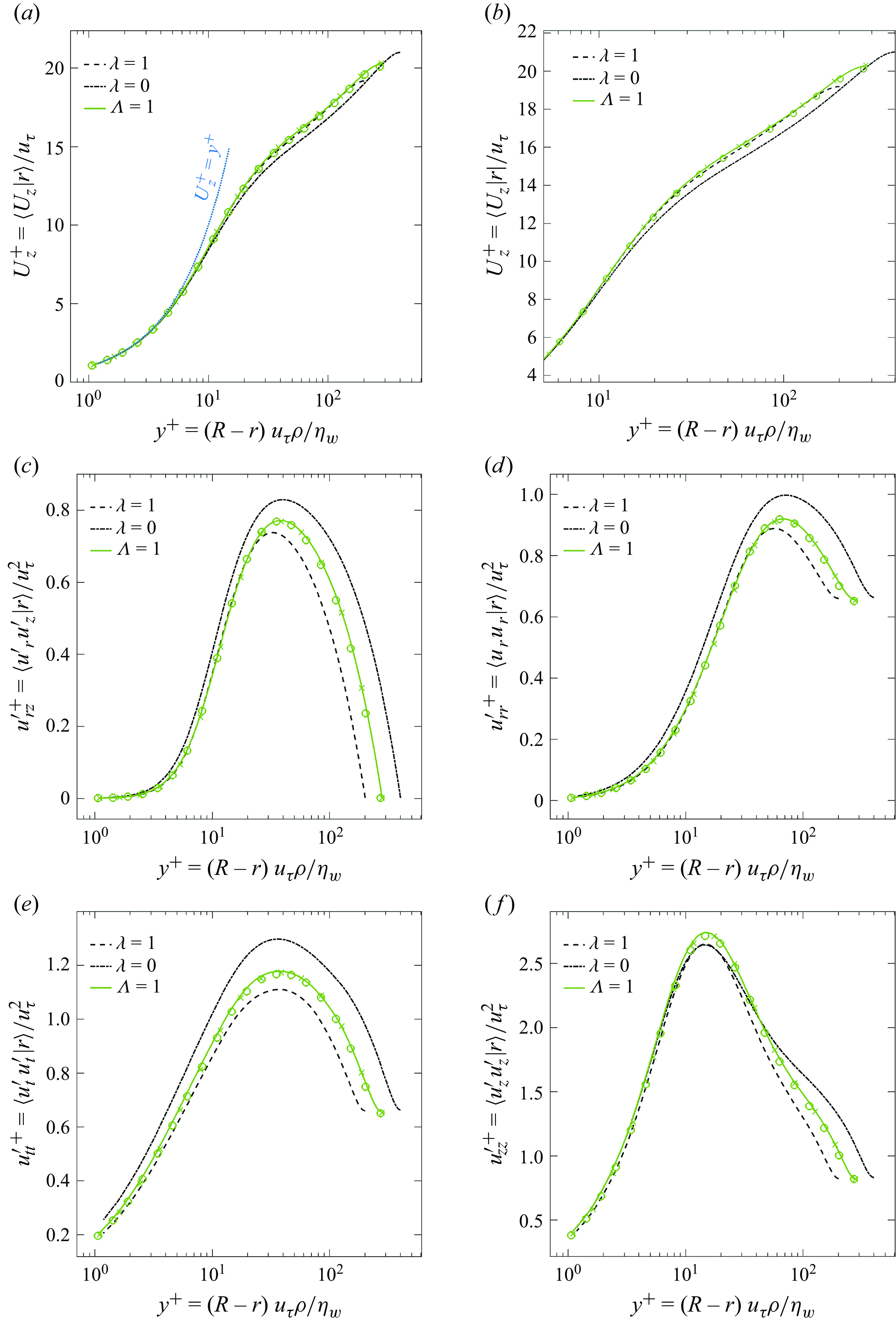
Figure 18. Mean velocity radial profiles (a–b) and Reynolds stresses (c–f) for thixotropic flows and Newtonian reference cases. The plots are from (solid lines) DNS results, (
![]() ) the effective viscosity model based on the conditionally averaged structural parameter
) the effective viscosity model based on the conditionally averaged structural parameter $\langle \lambda | r\rangle$
and (
$\langle \lambda | r\rangle$
and (
![]() ) the stochastic model (5.17).
) the stochastic model (5.17).
These results verify both the stochastic model for the averaged structural parameter $\langle \lambda |r\rangle$
and the effective viscosity model
$\langle \lambda |r\rangle$
and the effective viscosity model $\mu _{\textit{eff}}(r,\dot \gamma )$
for turbulent pipe flow. They also show that turbulent flow of time-dependent thixotropic fluids can be accurately approximated as time-independent GN fluids via the effective viscosity
$\mu _{\textit{eff}}(r,\dot \gamma )$
for turbulent pipe flow. They also show that turbulent flow of time-dependent thixotropic fluids can be accurately approximated as time-independent GN fluids via the effective viscosity $\mu _{\textit{eff}}(r,\dot \gamma )$
. Although it is somewhat surprising that such a simple stochastic model for
$\mu _{\textit{eff}}(r,\dot \gamma )$
. Although it is somewhat surprising that such a simple stochastic model for $\lambda$
and simple effective viscosity model
$\lambda$
and simple effective viscosity model $\eta _{\textit{eff}}$
can accurately capture the turbulent dynamics of a time-dependent fluid, it is important to note that unlike for example viscoelastic turbulence, purely thixotropic flow is still an essentially a viscous flow, albeit one with a non-local viscosity.
$\eta _{\textit{eff}}$
can accurately capture the turbulent dynamics of a time-dependent fluid, it is important to note that unlike for example viscoelastic turbulence, purely thixotropic flow is still an essentially a viscous flow, albeit one with a non-local viscosity.
Indeed, in the limit of fast $\Lambda \gg 1$
and slow
$\Lambda \gg 1$
and slow $\Lambda \ll 1$
thixotropic kinetics, the rheology of these fluids is time-independent (GN), while for intermediate kinetics
$\Lambda \ll 1$
thixotropic kinetics, the rheology of these fluids is time-independent (GN), while for intermediate kinetics $\Lambda \sim 1$
, the effective viscosity is well-approximated by the conditional average
$\Lambda \sim 1$
, the effective viscosity is well-approximated by the conditional average $\langle \eta |r\rangle$
, indicating that fluctuations of
$\langle \eta |r\rangle$
, indicating that fluctuations of $\eta$
around this mean are not important. As
$\eta$
around this mean are not important. As $\eta$
scales linearly with
$\eta$
scales linearly with $\lambda$
, figure 16(b) indicates that the variance of
$\lambda$
, figure 16(b) indicates that the variance of $\eta$
around
$\eta$
around $\langle \eta |r\rangle$
is significant for all
$\langle \eta |r\rangle$
is significant for all $r$
. However, the results above indicate that these variations do not significantly impact the structure of turbulent pipe flow.
$r$
. However, the results above indicate that these variations do not significantly impact the structure of turbulent pipe flow.
5.5. Nonlinear rheology and thixotropy
While we have considered simple linear rheological (2.9) and thixotropic (2.6) models in this study, the rheology and thixotropic kinetics of most complex fluids is highly nonlinear. Here we briefly consider the extension of the findings of this study to nonlinear rheology (2.3) and thixotropic models (2.4). These nonlinear models admit an equilibrium structural parameter $\lambda _{\textit{eq}}(\dot \gamma )$
given by (2.5), leading to the following viscosity model in the fast kinetic limit
$\lambda _{\textit{eq}}(\dot \gamma )$
given by (2.5), leading to the following viscosity model in the fast kinetic limit $(\Lambda \gg 1)$
as
$(\Lambda \gg 1)$
as
 \begin{equation} \lim _{\Lambda \rightarrow \infty }\eta (\lambda ,\dot \gamma )=\eta (\lambda _{\textit{eq}}(\dot \gamma ),\dot \gamma ), \end{equation}
whereas in the slow kinetic limit $(\Lambda \ll 1)$
we recover
$(\Lambda \ll 1)$
we recover
 \begin{equation} \lim _{\Lambda \rightarrow 0}\eta (\lambda ,\dot \gamma )=\eta (\lambda _{\textit{eq}}(\langle \dot \gamma \rangle ),\dot \gamma ). \end{equation}
For intermediate kinetics, if we again assume that the effective viscosity can be represented in terms of the radially averaged structural parameter, then
 \begin{equation} \eta (\lambda ,\dot \gamma )=\eta (\langle \lambda |r\rangle ,\dot \gamma ), \end{equation}
which recovers (5.40) and (5.41), respectively, in the limits $\Lambda \gg 1$
,
$\Lambda \gg 1$
, $\Lambda \ll 1$
.
$\Lambda \ll 1$
.
Although structural parameter models of the form (2.4) do not possess analytic solutions in general, their solution is still of the form of the shear history functional $\hat {\mathcal{F}}$
in (5.2). However, many nonlinear structural parameter models (Mewis & Wagner Reference Mewis and Wagner2009) can be expressed in non-dimensional form as
$\hat {\mathcal{F}}$
in (5.2). However, many nonlinear structural parameter models (Mewis & Wagner Reference Mewis and Wagner2009) can be expressed in non-dimensional form as
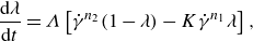 \begin{equation} \frac {{\rm d}\lambda }{{\rm d}t}=\Lambda \left [\dot \gamma ^{n_2}(1-\lambda )-K\dot \gamma ^{n_1}\lambda \right ], \end{equation}
where the index $n_2=0$
corresponds to Brownian rebuild, and
$n_2=0$
corresponds to Brownian rebuild, and $n_2\gt 0$
corresponds to shear-induced rebuild. These models have equilibrium solution
$n_2\gt 0$
corresponds to shear-induced rebuild. These models have equilibrium solution
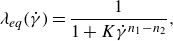 \begin{equation} \lambda _{\textit{eq}}(\dot \gamma )=\frac {1}{1+K\dot \gamma ^{n_1-n_2}}, \end{equation}
and so are shear thinning for $n_1\gt n_2$
and shear thickening for
$n_1\gt n_2$
and shear thickening for $n_1\lt n_2$
. This class of structural parameter model has explicit solution
$n_1\lt n_2$
. This class of structural parameter model has explicit solution
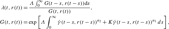 \begin{align} \lambda (t,r(t))&=\frac {\Lambda \int _0^\infty G(t-s,r(t-s)){\rm d}s}{G(t,r(t))},\nonumber\\ G(t,r(t))&=\exp \left [\Lambda \int _0^\infty \dot \gamma (t-s,r(t-s))^{n_2}+K\dot \gamma (t-s,r(t-s))^{n_1}\,ds\right ], \end{align}
and so the results derived in § 5.3 can be directly applied to these nonlinear models with $\langle \lambda |r\rangle$
given by (5.32) and
$\langle \lambda |r\rangle$
given by (5.32) and
 \begin{equation} h(r)=\exp \left [\Lambda \,\Delta s(\langle \dot \gamma |r\rangle ^{n_2}+K\langle \dot \gamma |r\rangle ^{n_1})\right ]. \end{equation}
Clearly, further research is required to justify the assumptions associated with the stochastic model for Lagrangian shear rate and effective viscosity model (5.3) for nonlinear viscosity $\eta (\lambda ,\dot \gamma )$
and thixotropy models.
$\eta (\lambda ,\dot \gamma )$
and thixotropy models.
6. Conclusions
In this study we have considered fully developed turbulent pipe flow of a time-dependent complex fluid, modelled via the simplest non-trivial thixotropic rheology model; a purely viscous Moore fluid (Moore Reference Moore1959) with structural parameter $\lambda$
. Despite this simplicity, these results are relevant to a broad class of applications involving inelastic thixotropic flow of materials with otherwise GN viscous rheology, and so are relevant to a wide class of industrial flows (pipelining, heat transfer, mixing, etc.) of complex materials including suspensions and emulsions, slurries, pastes and biological materials. The feedback between turbulence structure, rheology and microstructural state in these complex flows is not well understood.
$\lambda$
. Despite this simplicity, these results are relevant to a broad class of applications involving inelastic thixotropic flow of materials with otherwise GN viscous rheology, and so are relevant to a wide class of industrial flows (pipelining, heat transfer, mixing, etc.) of complex materials including suspensions and emulsions, slurries, pastes and biological materials. The feedback between turbulence structure, rheology and microstructural state in these complex flows is not well understood.
To address this shortcoming, we use DNS to simulate fully developed moderately turbulent flow ( $Re_G\approx 6,000-14,000$
) over a broad range of thixotropic kinetics from slow to fast (with respect to the advective time scale), as reflected by the thixoviscous numbers
$Re_G\approx 6,000-14,000$
) over a broad range of thixotropic kinetics from slow to fast (with respect to the advective time scale), as reflected by the thixoviscous numbers $\Lambda \in [10^{-2},10^{2}]$
. We consider transport of
$\Lambda \in [10^{-2},10^{2}]$
. We consider transport of $\lambda$
in the advection-dominated regime (
$\lambda$
in the advection-dominated regime ( $Pe=10^3$
), and note that for most complex fluids, self-diffusion of
$Pe=10^3$
), and note that for most complex fluids, self-diffusion of $\lambda$
is negligible (
$\lambda$
is negligible ( $Pe\sim 10^{12}$
).
$Pe\sim 10^{12}$
).
As expected, in the limit of fast thixotropic kinetics ( $\Lambda \gg 1$
), the viscosity of thixotropic fluids converges to that given by the equilibrium structural parameter
$\Lambda \gg 1$
), the viscosity of thixotropic fluids converges to that given by the equilibrium structural parameter $\lambda _{\textit{eq}}(\dot \gamma (\textbf{x},t))$
(2.7), and so the viscosity converges to the shear thinning case
$\lambda _{\textit{eq}}(\dot \gamma (\textbf{x},t))$
(2.7), and so the viscosity converges to the shear thinning case $\eta (\lambda ,\dot \gamma )=\eta (\lambda _{\textit{eq}}(\dot \gamma ,\dot \gamma )$
. In this limit, the turbulence structure of these flows is the same as that of a shear thinning GN fluid.
$\eta (\lambda ,\dot \gamma )=\eta (\lambda _{\textit{eq}}(\dot \gamma ,\dot \gamma )$
. In this limit, the turbulence structure of these flows is the same as that of a shear thinning GN fluid.
Conversely, in the limit of slow thixotropic kinetics ( $\Lambda \ll 1$
), the viscosity of thixotropic fluids converges to that given by the average structural parameter
$\Lambda \ll 1$
), the viscosity of thixotropic fluids converges to that given by the average structural parameter $\lambda _{\textit{eq}}(\langle \dot \gamma \rangle )$
(5.28) due to ergodic sampling of the shear rate along pathlines, and so the viscosity converges to
$\lambda _{\textit{eq}}(\langle \dot \gamma \rangle )$
(5.28) due to ergodic sampling of the shear rate along pathlines, and so the viscosity converges to $\eta (\lambda ,\dot \gamma )=\eta (\lambda _{\textit{eq}}(\langle \dot \gamma \rangle ,\dot \gamma )$
. In this limit, the turbulence structure of the Moore fluid is the same as that of a Newtonian fluid. In general, thixotropic fluids behave as GN fluids in this limit.
$\eta (\lambda ,\dot \gamma )=\eta (\lambda _{\textit{eq}}(\langle \dot \gamma \rangle ,\dot \gamma )$
. In this limit, the turbulence structure of the Moore fluid is the same as that of a Newtonian fluid. In general, thixotropic fluids behave as GN fluids in this limit.
Hence, in the limits of fast and slow thixotropic kinetics, turbulent flow of time-dependent inelastic thixotropic fluids is identical to that of turbulent flow of purely viscous time-independent fluids. For intermediate thixotropic kinetics, the picture is more complex as the local (in space and time) structural parameter $\lambda$
and hence viscosity
$\lambda$
and hence viscosity $\eta$
depends upon the Lagrangian history of shear rates.
$\eta$
depends upon the Lagrangian history of shear rates.
From the thixotropic kinetic equation, we derive an expression for local $\lambda$
as a ‘fading memory’ functional
$\lambda$
as a ‘fading memory’ functional $\mathcal{F}$
of the Lagrangian shear history where
$\mathcal{F}$
of the Lagrangian shear history where $\Lambda$
governs the persistence of memory in this functional. As fully developed pipe flow is non-stationary in the radial coordinate, we propose that turbulent thixotropic pipe flow with intermediate thixotropic kinetics (
$\Lambda$
governs the persistence of memory in this functional. As fully developed pipe flow is non-stationary in the radial coordinate, we propose that turbulent thixotropic pipe flow with intermediate thixotropic kinetics ( $\Lambda \sim 1$
) may be approximated as a purely viscous (time-independent) flow with radially variable effective viscosity given by the conditionally averaged structural parameter as
$\Lambda \sim 1$
) may be approximated as a purely viscous (time-independent) flow with radially variable effective viscosity given by the conditionally averaged structural parameter as $\eta (\lambda ,\dot \gamma )=\eta _{\textit{eff}}(r,\dot \gamma )\equiv \eta (\langle \lambda |r\rangle ,\dot \gamma )$
(5.39). This path integral formulation is completely general and applies to all
$\eta (\lambda ,\dot \gamma )=\eta _{\textit{eff}}(r,\dot \gamma )\equiv \eta (\langle \lambda |r\rangle ,\dot \gamma )$
(5.39). This path integral formulation is completely general and applies to all $\Lambda \in (0,\infty ^+)$
, recovering the previously derived closures for the fast and slow thixotropic kinetics.
$\Lambda \in (0,\infty ^+)$
, recovering the previously derived closures for the fast and slow thixotropic kinetics.
A stochastic model for $\eta _{\textit{eff}}$
can then be generated via a stochastic model for
$\eta _{\textit{eff}}$
can then be generated via a stochastic model for $\langle \lambda |r\rangle$
, which represents a path integral of the functional
$\langle \lambda |r\rangle$
, which represents a path integral of the functional $\mathcal{F}$
backwards in time over the Lagrangian shear histories that arrive at
$\mathcal{F}$
backwards in time over the Lagrangian shear histories that arrive at $r$
. We develop a simple non-stationary stochastic model for the Lagrangian shear history based on a Fokker–Planck equation for radial position (5.22) under the assumption that the instantaneous Lagrangian shear rate is given by the conditional average
$r$
. We develop a simple non-stationary stochastic model for the Lagrangian shear history based on a Fokker–Planck equation for radial position (5.22) under the assumption that the instantaneous Lagrangian shear rate is given by the conditional average $\dot \gamma =\langle \dot \gamma |r\rangle$
. This simple stochastic model provides accurate estimates of the conditionally averaged structural parameter
$\dot \gamma =\langle \dot \gamma |r\rangle$
. This simple stochastic model provides accurate estimates of the conditionally averaged structural parameter $\langle \lambda |r\rangle$
, and DNS computations based on this model for
$\langle \lambda |r\rangle$
, and DNS computations based on this model for $\Lambda =1$
agree with those given by the full thixotropic model to around 1% in terms of Reynolds stresses and mean axial velocity profile.
$\Lambda =1$
agree with those given by the full thixotropic model to around 1% in terms of Reynolds stresses and mean axial velocity profile.
Similarly, DNS computations based on direct computation of the conditionally averaged structural parameter $\langle \lambda |r\rangle$
from the full thixotropic DNS computations agree with these latter computations to a high degree of accuracy (
$\langle \lambda |r\rangle$
from the full thixotropic DNS computations agree with these latter computations to a high degree of accuracy ( $\sim$
2.4 % error for axial velocity and Reynolds stress profiles). These results establish that the turbulent flow of time-dependent thixotropic fluids is very similar to that of time-independent purely viscous (GN) fluids, for all ranges of thixotropic kinetics over the range
$\sim$
2.4 % error for axial velocity and Reynolds stress profiles). These results establish that the turbulent flow of time-dependent thixotropic fluids is very similar to that of time-independent purely viscous (GN) fluids, for all ranges of thixotropic kinetics over the range $\Lambda \in (0,\infty ^+)$
. For non-stationary flows such as fully developed turbulent pipe, this manifests as a radially dependent effective viscosity
$\Lambda \in (0,\infty ^+)$
. For non-stationary flows such as fully developed turbulent pipe, this manifests as a radially dependent effective viscosity $\eta _{\textit{eff}}(r,\dot \gamma )$
, whereas in general the effective viscosity is a function of every non-stationary direction of the flow. Similarly, homogeneous isotropic turbulent flow of thixotropic fluids are expected to behave in a similar manner to GN analogues, i.e.
$\eta _{\textit{eff}}(r,\dot \gamma )$
, whereas in general the effective viscosity is a function of every non-stationary direction of the flow. Similarly, homogeneous isotropic turbulent flow of thixotropic fluids are expected to behave in a similar manner to GN analogues, i.e. $\eta _{\textit{eff}}=\eta _{\textit{eff}}(\dot \gamma )$
.
$\eta _{\textit{eff}}=\eta _{\textit{eff}}(\dot \gamma )$
.
Although further research is required, these results suggest that they extend more broadly to a wide range of inelastic thixotropic fluids with nonlinear viscosity $\eta (\lambda ,\dot \gamma )$
and nonlinear thixotropic kinetics, as the basic mechanisms that govern the effective viscosity in these flows persist. The observation that under turbulent flow conditions, time-dependent thixotropic fluids behave as time-independent purely viscous analogues is a significant simplification that impacts a broad range of applications. This correspondence is attributed to the fact that thixotropic flows are viscous flows in terms of their stress–strain relationship (as opposed to for example viscoelastic flow), albeit ones with a non-local (Lagrangian history) viscosity dependence. The ergodic nature of turbulent flow appears to play an important role in rending these flows similar to time-independent purely viscous analogues. Future research involves investigation of the flow of more realistic (non-Newtonian) rheology models (see § 5.5 on the extension to nonlinear rheology) to assess whether the results remain consistent for larger viscosity ratios.
$\eta (\lambda ,\dot \gamma )$
and nonlinear thixotropic kinetics, as the basic mechanisms that govern the effective viscosity in these flows persist. The observation that under turbulent flow conditions, time-dependent thixotropic fluids behave as time-independent purely viscous analogues is a significant simplification that impacts a broad range of applications. This correspondence is attributed to the fact that thixotropic flows are viscous flows in terms of their stress–strain relationship (as opposed to for example viscoelastic flow), albeit ones with a non-local (Lagrangian history) viscosity dependence. The ergodic nature of turbulent flow appears to play an important role in rending these flows similar to time-independent purely viscous analogues. Future research involves investigation of the flow of more realistic (non-Newtonian) rheology models (see § 5.5 on the extension to nonlinear rheology) to assess whether the results remain consistent for larger viscosity ratios.
Funding
The authors acknowledge financial support from the Australian Research Council, Melbourne Water and Water Corporation, granted through ARC-Linkage 180100869. This research was also supported by the NCI Adapter Scheme, with computational resources provided by NCI Australia, an NCRIS-enabled facility supported by the Australian Government.
Declaration of interests
The authors report no conflict of interest.
Appendix A. Numerical method for thixotropic kinetics
The spectral element code (Blackburn et al. Reference Blackburn, Lee, Albrecht and Singh2019) employs a second-order temporal integration method (Karniadakis et al. Reference Karniadakis, Israeli and Orszag1991) based on the operator splitting technique. The advective nonlinear terms in the Navier–Stokes (2.14) and thixotropy (2.15) equations are treated explicitly, while the diffusion terms are handled implicitly to ensure numerical stability and convergence, as described in previous studies (Rudman & Blackburn Reference Rudman and Blackburn2006). To mitigate numerical instabilities, an implicit treatment of the reaction kinetics in (2.15) was implemented. The discretised reaction kinetics, derived from (4.3), are expressed as
 \begin{equation} \lambda _{n+1} = \frac {\lambda _n}{g_n(\Delta t)} + \frac {\Lambda }{\Lambda \left [1 + K \dot \gamma _n \right ]} \left [1 - \frac {1}{g_n(\Delta t)} \right ] ,\quad g_n(\Delta t) = \exp \left [\Lambda \Delta t \left (1+K\dot \gamma _n \right ) \right ], \end{equation}
where the subscript $n$
denotes quantities at time step
$n$
denotes quantities at time step $n$
. This formulation assumes that the local shear rate remains constant over a time step
$n$
. This formulation assumes that the local shear rate remains constant over a time step $\Delta t$
, i.e.
$\Delta t$
, i.e. $\dot \gamma (t) = \dot \gamma _n$
. This implicit treatment improves numerical stability and allows the code to handle the stiff terms effectively, even for high
$\dot \gamma (t) = \dot \gamma _n$
. This implicit treatment improves numerical stability and allows the code to handle the stiff terms effectively, even for high $\Lambda$
cases.
$\Lambda$
cases.


 Open access