The rotational transform and enhanced confinement in the TJ-II stellarator

Abstract

This study reports on a set of experiments designed to clarify the impact of the rotational transform on confinement quality at the TJ-II stellarator. For this purpose, the net plasma current is controlled using external coils, resulting in the modification of the rotational transform profile. Significant and systematic variations of the edge electron density gradients (up to $50\,\%{-}60\,\%$) and the plasma energy content ($20\,\%{-}30\,\%$) are achieved. The explanation of this behaviour relies on the placement of low-order rational surfaces in relation to the edge gradient region, which affect local turbulence fluctuation levels, facilitating the formation of zonal flows and concomitant transport barriers. This hypothesis is confirmed experimentally on the basis of a broad array of diagnostic measurements. Calculations based on a resistive magnetohydrodynamic turbulence model provide qualitative support for this hypothesis, clarifying the impact on confinement of specific rational surfaces and highlighting the complex nature of magnetically confined fusion plasmas.

1. Introduction

On the road to fusion energy as a power source for humanity, disposing of mechanisms to control the energy confinement quality of magnetically confined fusion plasmas by external means is highly desirable.

A significant body of literature has established that the rotational transform profile has an impact on energy confinement and H-mode access in low-shear stellarators. Experimentally, this is reflected in systematic changes of energy confinement with, for example, the edge rotational transform value. The now defunct stellarator W7-AS has delivered perhaps the most detailed study to date (Hirsch et al. 2008), while similar results were obtained at Heliotron-J and TJ-II, among others (Ascasíbar et al. 2008). More recent work at the optimised stellarator W7-X points in the same direction (Andreeva et al. 2022; Chaudhary et al. 2024).

These effects stand out particularly in the case of low-shear stellarators, where magnetohydrodynamic (MHD) turbulence plays an important role in particle and energy transport (Ida 2019). This type of turbulence is directly linked to the rotational transform, while low-order rational surfaces are well separated spatially in view of the low shear, which allows assessing the impact of individual rationals. Nevertheless, since MHD turbulence and modes are ubiquitous in magnetic confinement devices, the mentioned effects are expected to extend beyond the realm of low-shear stellarators. A case in point is provided by internal transport barriers, which often form in close association with a low-order rational surface in both stellarators and tokamaks (Wolf 2003; Motojima et al. 2003; Connor et al. 2004; Kenmochi et al. 2020). In so-called reversed-shear tokamak discharges, in which the safety factor profile $q(r)$ has an off-axis minimum, the rarefaction of rational surfaces near the minimum, when it is close to a low-order rational value, may facilitate a local reduction of transport (Austin et al. 2006; Garbet et al. 2010). Also, recent work at ASDEX-Upgrade (Willensdorfer et al. 2024) shows that islands and low-order rationals may impact transport in the plasma edge significantly.

In previous work (van Milligen et al. 2024) we studied a large collection of L–H transitions in the TJ-II stellarator, with different vacuum magnetic configurations, in order to answer the question ‘at what values of the net plasma current, $I_{\!p}$ , do L–H transitions tend to occur?’. Perhaps surprisingly, a systematic dependence of the occurrence of L–H transitions on the value of $I_{\!p}$ was observed. The cited work also suggested an explanation for this phenomenon. Namely, a net plasma current modifies the rotational transform profile, shifting the radial location of low-order rational surfaces in the plasma edge region. When $I_{\!p}$ is such that an important low-order rational surface is placed near $\rho \simeq 0.8$ (i.e. the foot of the density gradient region), it may facilitate the formation of associated zonal flows near that location, which in turn may facilitate the formation of a transport barrier and a transition to improved confinement.

To shed further light on this mechanism, the present work focuses on experiments performed in a single magnetic configuration. The particular configuration of interest was selected on the basis of the mentioned previous work (van Milligen et al. 2024). The configuration labelled ‘100_48_65’ with helical current $10\times I_{HX} = 48$ kA was not included in that work, but the observed trends of confinement improvement as a function of the net plasma current $I_{\!p}$ led us to expect significantly enhanced confinement for both positive and negative values of $I_{\!p}$ , but less so for small values.

The present analyses focus on the high-density phase with heating by neutral beam injection (NBI). In some experiments, plasma density was increased further using pellet injection, pushing the plasma more clearly into an enhanced confinement state (García-Cortés et al. 2023). We varied the plasma current over a significant range using external control coils. This induced a corresponding variation of the rotational transform profile. We then observed the resulting plasma state using a wide variety of diagnostics available at TJ-II. The results, reported here, reveal a systematic and reproducible relationship between the rotational transform profile and confinement. Moreover, the present novel results confirm the expectations based on previous work, namely confinement enhancement for both positive and negative values of the net plasma current in this particular configuration. The fulfilment of this expectation provides a strong confirmation of the underlying idea that confinement enhancement is related to the presence of rational surfaces in the edge region.

These experimental results find support from resistive MHD turbulence calculations. In this framework, we note that recent work at LHD (Kinoshita et al. 2024) highlights the importance of resistive MHD calculations for understanding magnetic confinement properties. In the turbulence calculations, the rotational transform profile is varied in a way similar to that in the experiment, using $I_{\!p}$ as a parameter. The main trends of edge gradients and effective confinement as a function of the parameter $I_{\!p}$ fully mirror the experimental results, and allow understanding of the impact of rational surfaces on confinement.

This article is organised as follows. Section 2 discusses the methods we have used. Section 3 presents experimental results. Section 4 presents the results from a numerical turbulence simulation that facilitates interpretation of the experimental results. In § 5 we discuss the results and in § 6 we draw some conclusions.

2. Methods

The experiments reported here are performed at the TJ-II stellarator (Harris et al. 1985), a flexible Heliac with toroidal magnetic field $B_T \simeq 1$ T, major radius $R_0 = 1.5$ m and minor radius $a \lt 0.22$ m (Hidalgo et al. 2022). TJ-II disposes of two electron cyclotron resonance heating (ECRH) beam lines, operating at 53.2 GHz, delivering up to about 300 kW of power each, and two tangential NBI systems, one injecting in the co-direction (with respect to the magnetic field) and one in the counter-direction (Liniers et al. 2013), injecting up to ${\sim}1$ MW of throughput power at up to $32$ keV into the TJ-II vessel for up to $120$ ms. Plasmas are initiated using ECRH, followed by an NBI heated phase. In this NBI phase, cryogenic pellets can be injected to raise the density.

The vacuum magnetic configuration is defined by the currents flowing in the external coil sets of TJ-II, and is identified by a label, xxx_yy_zz, consisting of three numbers proportional to the mentioned currents. The present work focuses on the magnetic configuration 100_48_65, a configuration of special interest, as mentioned in § 1. Error sources affecting the magnetic field configuration are discussed in van Milligen et al. (2011). One important conclusion from the latter paper is that the modification of the flux surface geometry due to finite pressure is typically minimal in the presence of plasma, whereas the modification of the rotational transform profile due to plasma currents may be significant.

The TJ-II stellarator is equipped with a large number and wide range of passive and active diagnostic systems (McCarthy & TJ-II team 2021), some of which are used in the analyses below.

2.1. Ohmic current control

In these experiments, the external Ohmic (OH) current coils (Romero et al. 2003) were used to control the toroidal plasma current. The total plasma current depends both on currents driven by the heating systems in combination with the plasma response, and on the externally induced magnetic flux variation generated by a variation of the current in the external OH coils. Direct feedback of the plasma current was attempted but not found to be feasible due to the long reaction times of the coil control system, in excess of 20 ms, and a predictive model was used instead (see Appendix A). This system allowed varying the plasma current in a significant range, as shown in the experimental section below (figure 2).

2.2. The impact of the net plasma current on the rotational transform

At TJ-II, the vacuum rotational transform profile generally provides a good approximation to the rotational transform profile in the presence of plasma, ${{\unicode{x0335}\mskip-3.5mu\iota} }(\rho ) = \iota (\rho )/2\pi$ , since the normalised plasma pressure $\beta$ is low, provided net currents are small (van Milligen et al. 2011). The vacuum rotational transform profile is obtained from VMEC calculations (Hirshman & Whitson 1983). The rotational transform profile is modified by the plasma current, $I_{\!p}$ , as explained in van Milligen et al. (2024). At present, we do not dispose of a proven method to determine the rotational transform experimentally with any degree of accuracy in TJ-II. However, an estimation of the radial distribution of the plasma current can be made assuming Spitzer resistivity (Castejón et al. 2004). Based on this assumption, a simplified model can be formulated to estimate the rotational transform profile in the presence of a net plasma current (Melnikov et al. 2014):

(2.1) \begin{equation} {\unicode{x0335}\mskip-3.5mu\iota}_{\textrm{plasma}} = {\unicode{x0335}\mskip-3.5mu\iota}_{\textrm{vacuum}} + C(\rho )I_{\!p}, \end{equation}

where $C(\rho ) = A \exp (-\rho /B)$ with $A=0.1107$ (kA) $^{-1}$ and $B=0.3557$ . Figure 1 (left) shows how the rotational transform is modified by a net plasma current, $I_{\!p}$ , according to this model, for the vacuum configuration considered in this paper.

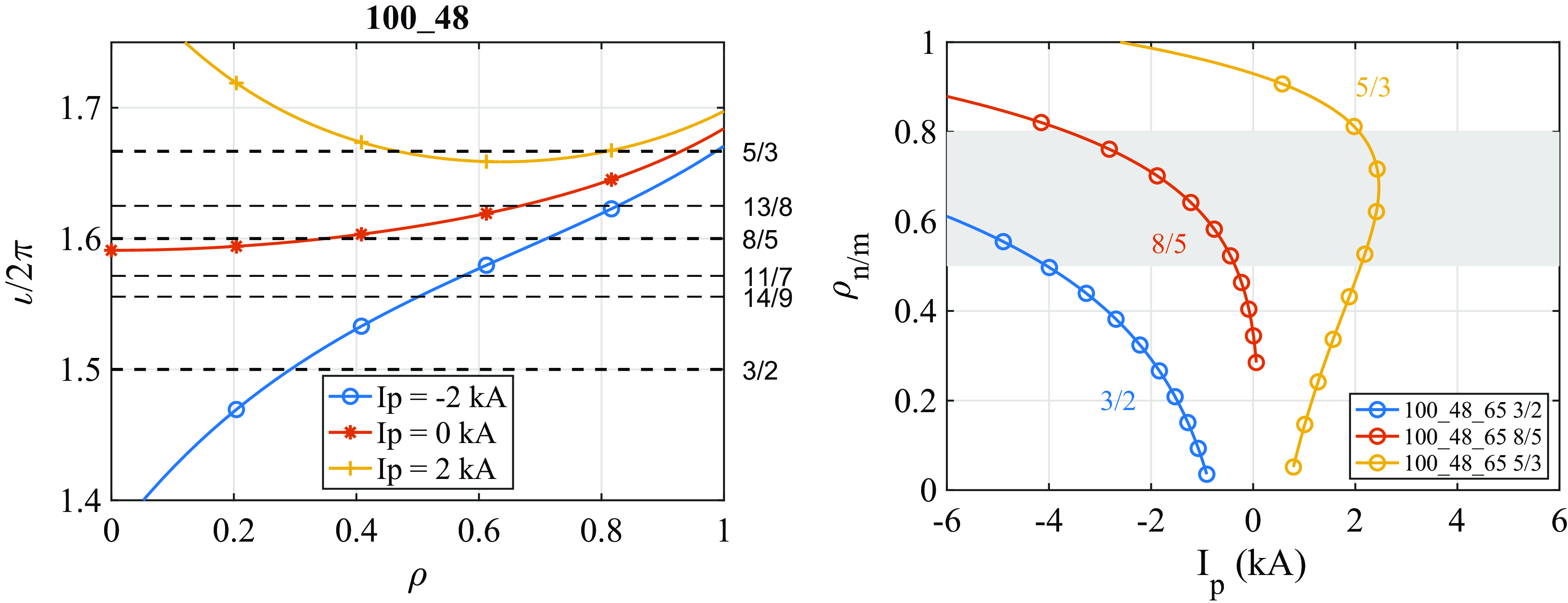
Figure 1. Left: relevant rotational transform profiles for configuration 100_48_65, in vacuum and for a few non-zero values of $I_{\!p}$ , according to the model of (2.1). All rationals ${\unicode{x0335}\mskip-3.5mu\iota} = n/m$ in the range $1.5 \leqslant {\unicode{x0335}\mskip-3.5mu\iota} \leqslant 1.7$ having $n\leqslant 15$ are shown as horizontal dashed lines, labelled on the right. Right: radial location of a few low-order rational surfaces for the magnetic configuration considered here, as a function of $I_{\!p}$ , according to the model of (2.1).

This model has had some success in the framework of modelling the temporal variation of Alfvén mode frequencies in TJ-II, as the plasma current evolved (Melnikov et al. 2014). We note that it is similar to a model that was used in W7-AS (Hirsch et al. 2008). Due to the fact that the magnetic field on a magnetic flux surface depends on the integral of the plasma current within the surface, and the total net plasma current is measured and known (see § 2.5), the model prediction is accurate near the plasma edge but rather uncertain in the plasma core, in the absence of experimental information on the radial current distribution.

This model allows us to understand, in approximation, in what way net plasma currents modify the radial location of rational surfaces. In the range $1.4 \lt {{\unicode{x0335}\mskip-3.5mu\iota} } \lt 1.75$ shown in figure 1 (left), the only rationals ${{\unicode{x0335}\mskip-3.5mu\iota} } = n/m$ having $n\lt 10$ correspond to $n/m \in \{3/2, 8/5, 5/3\}$ , and these are particularly important in this work.

Figure 1 (right) shows where these main low-order rational surfaces are located as a function of the parameter $I_{\!p}$ , according to the model. In this figure, the grey area indicates the approximate location of the ‘density gradient region’. It extends roughly from $\rho \simeq 0.5$ to $\rho \simeq 0.8$ (see § 3.2). The gradient region is important because MHD turbulence and modes, associated with the rational surfaces, are driven more strongly where the gradient is high.

The figure shows the predicted radial location of the mentioned three low-order rationals, {3/2, 8/5, 5/3}, for magnetic configuration 100_48_65 and for a range of plasma currents, $-6 \leqslant I_{\!p} \leqslant 6$ kA. For $I_{\!p} \lt -4$ , the 3/2 surface may enter the gradient region. In the interval $-3 \lt I_{\!p} \lt 0$ kA, the 8/5 surface may be located in the gradient region. In the interval $0 \lt I_{\!p} \lt 2$ kA, none of the three mentioned rationals are located in the gradient region. For $2 \lt I_{\!p} \lt 2.5$ , the 5/3 surface may enter the gradient region. The radial variation of the location of these rational surfaces as a function of $I_{\!p}$ is quite significant, which means that it is important to consider the effect of $I_{\!p}$ in order to understand the impact of the location of rational surfaces on confinement.

One also observes that the 5/3 rational surface, in particular, may occur twice in the plasma region for $2 \lt I_{\!p} \lt 2.5$ , due to the fact that the ${\unicode{x0335}\mskip-3.5mu\iota}$ profile ‘curves upward’ for sufficiently large positive values of $I_{\!p}$ , as seen in figure 1 (left). This is not true for the 3/2 and 8/5 surfaces, always corresponding to a single radius only for this configuration.

We emphasise that the model is approximate and we will use it mainly to help interpret the observations, reported below, in the absence of an actual direct measurement of the rotational transform profile. Apart from the systematic error involved (i.e. the assumed radial distribution of the plasma current), the inferred radial positions of rational surfaces are also subject to measurement errors of the total plasma current. Namely, according to the model, $|{\rm d}\rho _{n,m}/{\rm d}I_{\!p}|$ is small in the edge and large in the core (figure 1 (right)), which implies a certain reliability of the radial placement of rationals in the edge region, but a significant unreliability in the core, due to the propagation of the error in $I_{\!p}$ . In this work, our main concern will be with rational surfaces in the edge region.

2.3. Pellet injection

The TJ-II pellet injector can deliver up to four pellets per discharge (Combs et al. 2013). The pellets are small, with a diameter between 0.5 and 1 mm, and they are injected into the plasma at speeds of up to 1 km s⁻¹. In high-temperature plasmas heated by ECRH, the pellets are fully ablated before reaching the plasma centre. In plasmas heated by NBI, with slightly lower temperatures, the pellets can penetrate further (McCarthy et al. 2021) and most of the material is subsequently deposited at the plasma centre (Panadero et al. 2018).

The beneficial effect of pellets on TJ-II plasma performance has been described in García-Cortés et al. (2023) and McCarthy et al. (2024). With NBI heating, deep fuelling stabilises the plasma energy content at record levels. In plasmas without pellet injection, the energy confinement time typically lies in the range $\tau _E \simeq 5{-}10$ ms. However, during discharges with pellet injection, $\tau _E$ can easily reach 15 ms, significantly exceeding the prediction of the ISS04 scaling law using the TJ-II renormalisation factor (Yamada et al. 2005).

2.4. Profiles

TJ-II disposes of a high-resolution ( $2{-}6$ mm) Thomson scattering system that allows the reconstruction of the electron density and temperature profiles along a chord traversing the plasma (Barth et al. 1999). The system delivers only a single profile measurement for each discharge, so the selection of the time of interest is important. A helium beam system allows measuring the electron density and temperature at several (up to 16) points along a chord in the plasma edge and scrape-off layer regions (Hidalgo et al. 2004). For more information on the reconstruction of the electron density profile using various diagnostics at TJ-II, the reader is referred to van Milligen et al. (2011).

From the measured or estimated profiles, an approximate value of the thermal energy content can be obtained:

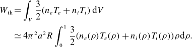(2.2) \begin{align} W_{\textrm{th}} & = \int _V{\frac 32 (n_eT_e+n_iT_i)\,\mathrm{d}V} \nonumber \\ &\simeq 4 \pi ^2a^2R \int _0^1{\frac 32(n_e(\rho )T_e(\rho )+n_i(\rho )T_i(\rho ))\rho \mathrm{d}\rho }. \end{align}

Here, we take the major radius $R=1.5$ m and the minor radius $a=0.22$ m. The normalised radial coordinate is $\rho = r/a$ .

2.5. Magnetic diagnostics

TJ-II is fitted with a Rogowski coil to measure the toroidal plasma current, $I_{\!p}$ , and a diamagnetic loop that is used to measure the diamagnetic plasma energy content, $W_{\textrm{dia}}$ (Ascasíbar et al. 1999, 2010). However, it is known that the measurement of $W_{\textrm{dia}}$ at TJ-II is affected by the net plasma current (Ascasíbar et al. 2005). Since in this work we intentionally vary the plasma current, we will base our conclusions on the thermal energy content $W_{\textrm{th}}$ (see § 2.4), as this quantity is robust against any influence from $I_{\!p}$ .

Three arrays of Mirnov coils are installed in TJ-II (Ascasíbar et al. 2022). The so-called poloidal array measures only one component of the field at each position and is indicated for the measurement of the poloidal mode number $m$ while the other two are helical sets of triaxial coils that measure the three components of the magnetic field at each position and are used to determine the toroidal mode number $n$ , once $m$ has been found. In the framework of the three-dimensional Lomb periodogram technique, the spatial position of each coil is mapped to the magnetic coordinates of its closest location on the last closed flux surface. Since each helical array follows a straight line in magnetic coordinates, the measured signals depend on both the toroidal and the poloidal mode numbers of the analysed perturbation. This link between poloidal and toroidal structure produces different pairs of values of $m$ and $n$ , for which the result for the periodogram is the same. These pairs are distributed along a line in the $n, m$ space that satisfies $n-Nm=l$ , where $N$ is the device period and $l$ is a constant that depends on the specific mode. Similar behaviour, although much less dependent on the toroidal mode number, appears when the signals of the poloidal array are analysed with the three-dimensional periodogram technique. Since the coils of the poloidal array have different toroidal magnetic angles, a slight dispersion in valid values of $m$ arises. Only by combining the measurements of all the arrays can we determine a definite pair of mode numbers. The analysis method and its subtleties are described in detail in Pons-Villalonga et al. ( 2025).

2.6. Doppler reflectometry

We use Doppler reflectometry to obtain information about the edge radial electric field, $E_r$ , and electron density turbulence levels in the plasma edge region (Estrada et al. 2010; Happel et al. 2011). The diagnostic launches its microwave beam into the plasma at an oblique angle, while the beam disposes of two separate beam frequencies, so that the beam reflection layer is located at two different radial positions. Depending on the density profile, the channel locations typically correspond to $\rho \simeq 0.8$ (channel 1) and $\rho \simeq 0.7$ (channel 2). These locations are typically close to the position where the edge transport barrier (if any) tends to form.

2.7. Heavy ion beam probe

TJ-II disposes of a dual heavy ion beam probe (HIBP) system (Melnikov et al. 2017). The two systems, similar but placed at different toroidal locations, are capable of simultaneously measuring, among others, the plasma potential and the electron density, at various closely spaced locations or sampling volumes, with a high sampling rate that allows turbulence analyses (1 MHz). The sampling volumes can be held fixed or scanned though the plasma, from one edge (low-field side) to the opposite edge (high-field side), in scans typically lasting between 10 and 60 ms, according to requirement.

2.8. Resistive MHD turbulence model

In an effort to understand the influence of low-order resonant surfaces on confinement enhancement in the TJ-II, we perform turbulence calculations using a resistive MHD model derived from the reduced MHD equations (Strauss 1976; García et al. 2001). In this simplified approach, interchange modes are the primary instability. The average equilibrium magnetic field has cylindrical symmetry, while the magnetic field line curvature is captured by means of an average magnetic field line curvature term. Since the model does not account for the full three-dimensional magnetic structure of the TJ-II stellarator, it does not provide a precise simulation of the TJ-II experiments. However, it has proven its usefulness for the qualitative interpretation of experimental results in recent studies (van Milligen et al. 2017; van Milligen & Sánchez 2022; van Milligen et al. 2023). A detailed description of the model and its key parameters can be found in García et al. (2001, 2023). The parameters used include $n_{e0} = 3\times 10^{19}$ m $^{-3}$ , $T_{e0} = 0.3$ keV and $B_0 = 1.1$ T, with the rotational transform profile taken from (2.1). In the calculations for magnetic configuration 100_48_65 of the TJ-II stellarator presented here, we have used normalised pressure at the magnetic axis $\beta _0 = 0.003$ , inverse aspect ratio $\epsilon =a/R_0= 0.15$ , resistive time at the magnetic axis $\tau _R=0.1$ s and Lundquist number $S = \tau _R/\tau _A = 2 \times 10^5$ . Given this choice of parameters and profile shapes similar to the experimental ones, this configuration is unstable to resistive interchange modes, and the use of a resistive MHD model is justified at least in the plasma core and gradient regions, as the mean free path is much smaller than the typical length of filaments in TJ-II (van Milligen et al. 2013). The purpose of the model is not to replicate the experimental specifics, but rather to shed light on the impact of low-order rational surfaces on confinement.

3. Experimental results

This work presents results from experiments performed on 9 May 2024, in magnetic configuration 100_48_65. Heating was performed with one NBI heating system (counter-NBI). Predictive $I_{\!p}$ current control was used to control the net plasma current (see § 2.1). The dataset includes discharges with and without pellet injection. In a few discharges, two successive pellets were injected.

Discharges with NBI heating but without pellet injection may present L–H confinement transitions, characterised by an increase in plasma density and plasma energy content, a reduction in $H_\alpha$ emission from the edge, the development of steep edge density gradients and a reduction in the turbulence level (Estrada et al. 2010). The injection of pellets into such discharges may induce an additional bifurcation, enhancing confinement further (García-Cortés et al. 2023).

According to van Milligen et al. (2024), in configuration 100_48_65, L–H confinement transitions are expected at both $I_{\!p} \simeq 2$ kA (with the 5/3 rational at $\rho \simeq 0.8$ ; see figure 1 (right)) and $I_{\!p} \simeq -1.5$ kA (with the 13/8 rational at $\rho \simeq 0.8$ ) and/or at $I_{\!p} \simeq -3.5$ kA (with the 8/5 rational at $\rho \simeq 0.8$ ) – noting that the cited paper did not contemplate such strongly negative net currents, as only spontaneously generated currents were considered. An initial goal of the present work is to confirm this expectation.

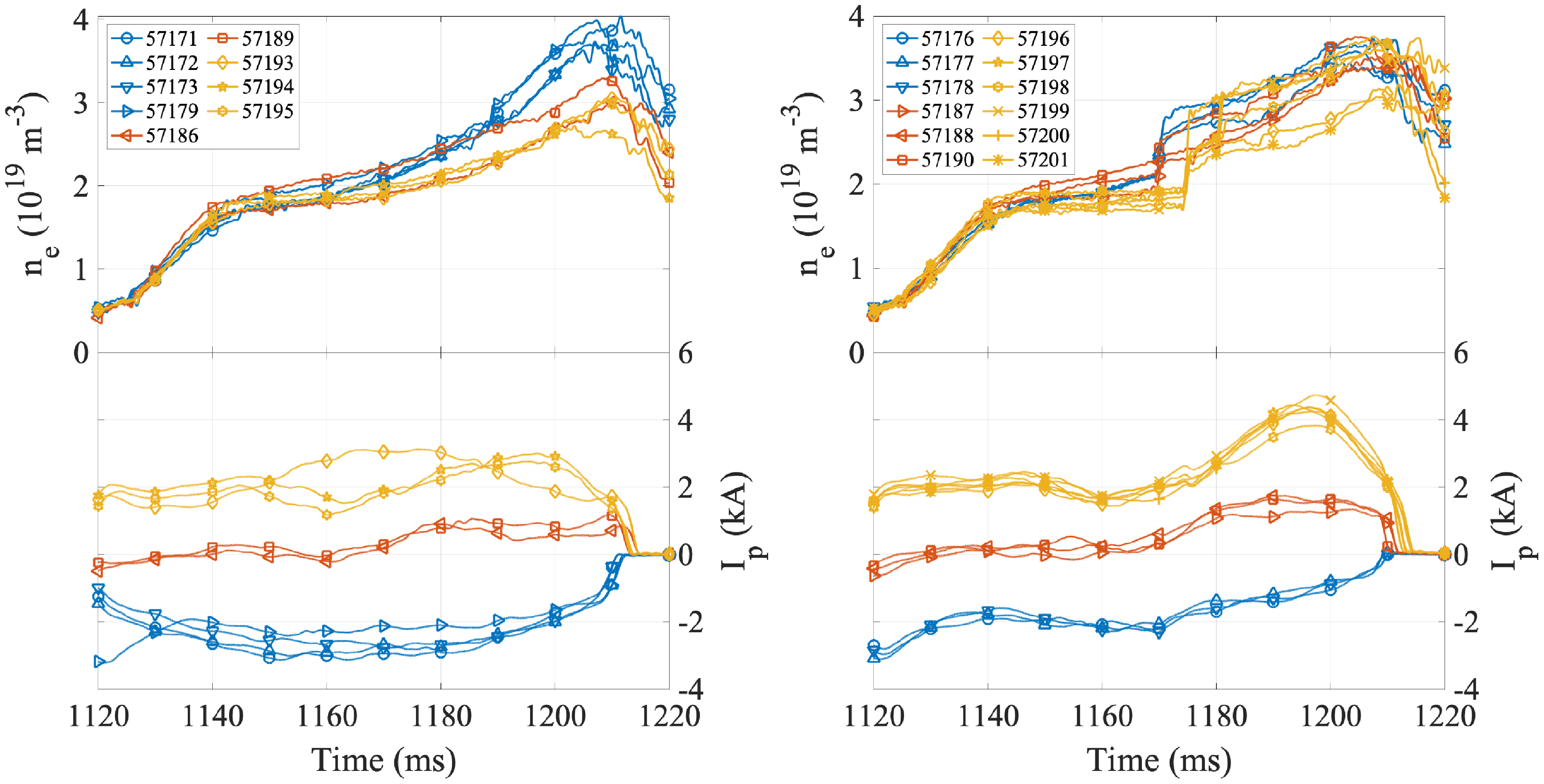
Figure 2. Time traces without (left) and with (right) pellet injection. Top: line average density; bottom: net plasma current. Colours indicate the target values of the plasma current $I_{\!p}$ (shown in the bottom panel). Symbols mark different discharges.

3.1. Current control

Some time traces of the discharges of this experimental day are shown in figure 2. The net plasma current (lower panel) was controlled by external means (see § 2.1 and Appendix A). While the applied current control was not perfect, as the target $I_{\!p}$ values were set at $-2,\ 0$ and $2$ kA, still a good variation of $I_{\!p}$ was obtained, and the resulting discharges were reasonably reproducible. The plasma current showed a moderate but systematic increase following the time of pellet injection ( $1170 \lt t_{p} \lt 1180$ ms), in accordance with expectations from simulations regarding the concomitant modification of the slowing-down time of fast ions (Mulas et al. 2022). Namely, following the pellet, the increased density and reduced temperature result in a reduction of the negative contribution to the total current due to counter-NBI, and this results in an increase of the total current. Apart from this non-diffusive current effect, the net plasma current is fairly constant in the time window of interest and, given the resistive time scale of $\tau _R \simeq 10{-}20$ ms, current diffusion effects are not expected to play a major role.

3.2. Electron density and temperature profiles

Figure 3 shows average electron density profiles obtained using Thomson scattering inside the plasma (Thomson scattering $n_e$ values were recalibrated against the interferometer using non-pellet discharges) and the helium beam in the far edge and scrape-off layer regions. Similarly, figure 4 shows the corresponding average electron temperature profiles. Individual profiles correspond to the times the Thomson scattering laser was fired, here always in the range $1180 \leqslant t \leqslant 1190$ ms, near but not necessarily at the time of maximum energy content, $W$ . The shown profiles have been averaged over similar discharges with approximately the same net plasma current, as listed individually in figure 2. The values of $I_{\!p}$ indicated in the plot legends are the target $I_{\!p}$ values, not the actual value of $I_{\!p}$ achieved at the Thomson scattering time.

Figure 3. Averaged Thomson scattering ( $\bigtriangledown$ ) and helium beam ( $\bigcirc$ ) electron density profiles, without (left) and with (right) pellet injection. The profiles have been averaged over similar discharges with approximately the same net plasma current, as listed in figure 2. The Thomson scattering laser time was in the range $1180 \leqslant t \leqslant 1190$ ms. The legend indicates the target plasma current $I_{\!p}$ corresponding to each profile, also indicated by line colour (same colour as in the cited figure).

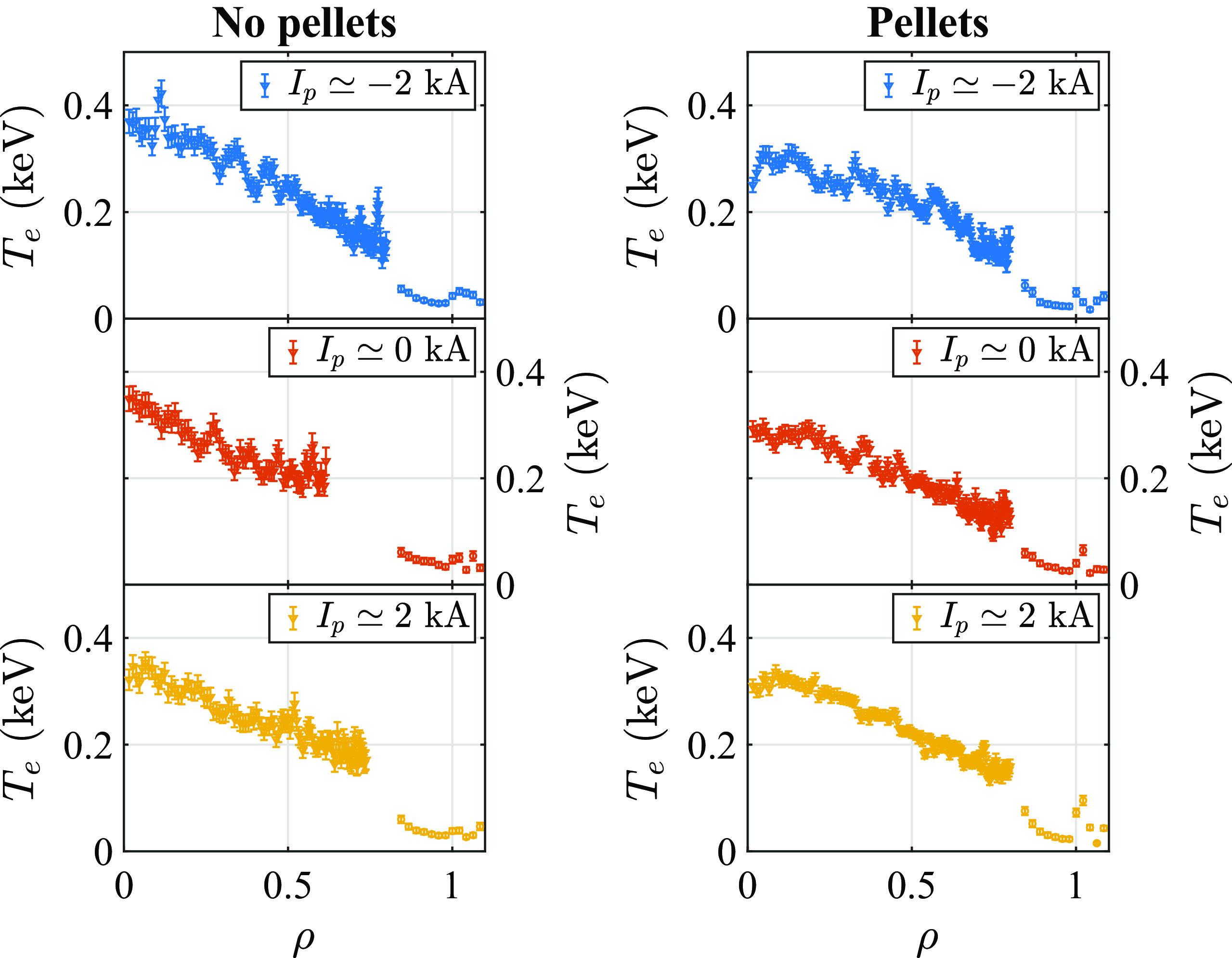
Figure 4. Averaged Thomson scattering ( $\bigtriangledown$ ) and helium beam ( $\bigcirc$ ) electron temperature profiles, without (left) and with (right) pellet injection. The profiles have been averaged over similar discharges with approximately the same net plasma current, as listed in figure 2. The Thomson scattering laser time was in the range $1180 \leqslant t \leqslant 1190$ ms. The legend indicates the target plasma current $I_{\!p}$ corresponding to each profile, also indicated by line colour (same colour as in the cited figure).

The central density in the discharges with pellets is only slightly higher than in the discharges without pellets, but the profile is significantly broader and the density gradient is significantly higher (locally, in the ‘gradient region’ $0.5{-} 0.6 \lt \rho \lt 0.8$ ; the interior boundary of this region being less sharply defined than the exterior boundary). These enhanced gradients can be related to higher confinement (as shown below). Temperature profiles in the discharges with and without pellets reach peak values of $0.3{-}0.4$ keV in the core.

With pellets and $I_{\!p} \simeq -2$ kA, one observes a relatively steep density gradient at $0.67 \lt \rho \lt 0.79$ , essentially coincident with the predicted location of the 8/5 rational ( $\rho _{8/5} \simeq 0.7$ , cf. figure 1 (left)). Likewise, with pellets and $I_{\!p} \simeq 2$ kA, one observes a relatively sharp density gradient at $0.65 \lt \rho \lt 0.84$ , when the 5/3 rational is predicted to occur near $\rho \simeq 0.8$ , as well as near $\rho \simeq 0.5$ (cf. figure 1 (right)) – noting that the estimate of the inward position of this rational surface is prone to large error. In any case, this relative steepening of the gradient is also visible in the no-pellet cases, although much less pronounced and less clearly localised.

In the case of the electron temperature profiles (figure 4), it should be noted that the Thomson scattering $T_e$ measurements are not reliable in the gradient region for low-edge-density shots (without pellets) due to high noise levels; the corresponding noisy points have been omitted. However, in the high-edge-density (pellet) cases, one observes a clear steepening of the edge temperature profiles near $\rho \simeq 0.8$ for positive $I_{\!p}$ , likely associated with the 5/3 rational that is predicted to occur at that location.

The impact of the current on the edge electron density gradient is quantified in figure 5 (left), which shows the slope of the Thomson scattering density profile, calculated from a linear fit to the mean profile (averaged over similar discharges, as shown in figure 3) in the radial interval $0.65 \leqslant \rho \leqslant 0.8$ . The error bars correspond to the square root of the variation of values obtained in different discharges, thus reflecting the combined effect of variations in plasma conditions and measurement error. The lowest density gradients correspond to the cases with $I_{\!p} \simeq 0{-}2$ kA, both with and without pellets, whereas the density gradient increases both for negative and sufficiently large positive currents. The injection of pellets enhances the density gradient by a factor of about 2 (for all values of the current).

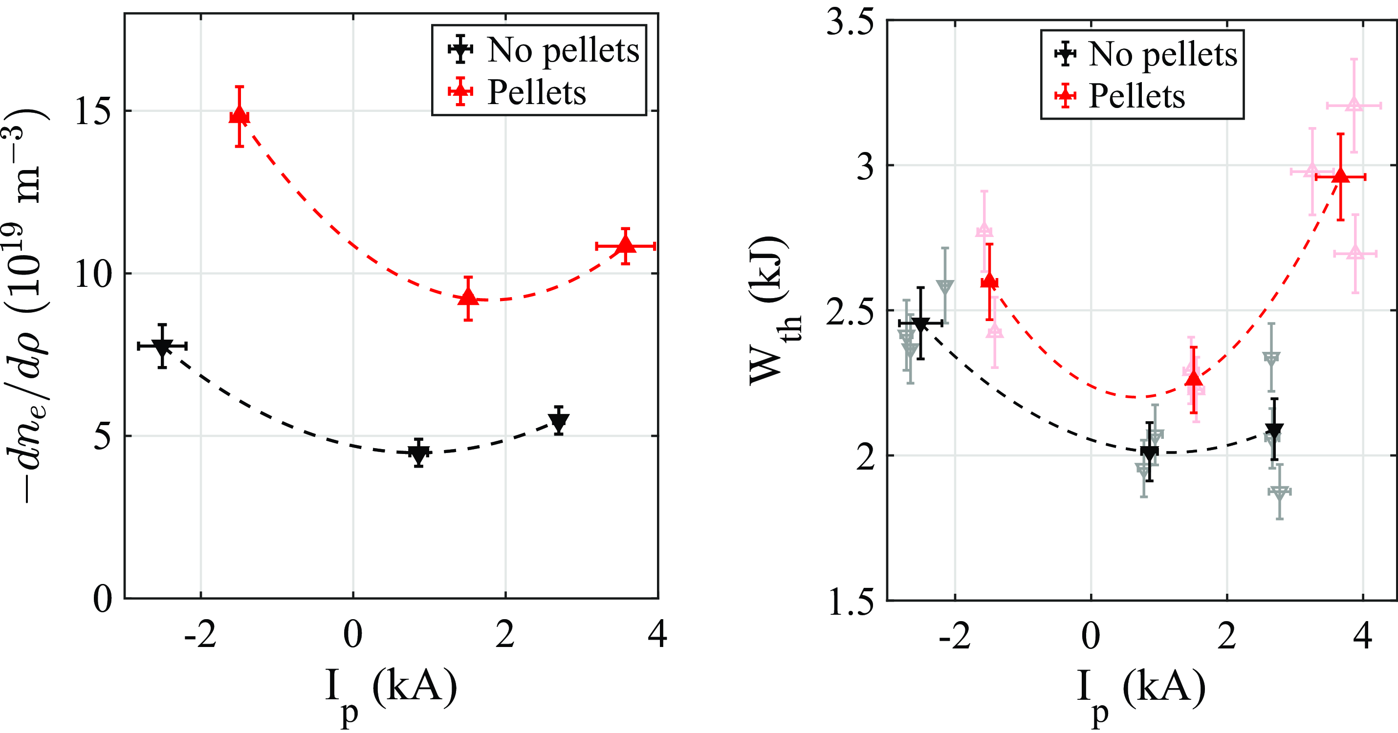
Figure 5. Left: slope of the mean Thomson scattering density profile in the radial interval $0.65 \leqslant \rho \leqslant 0.8$ . Right: $W_{\textrm{th}}$ versus $I_{\!p}$ , for (black) the discharges without pellets and (red) the discharges with pellets. Data from individual discharges are shown using light-coloured open symbols; averages over sets of discharges with similar $I_{\!p}$ are shown using dark-coloured filled symbols. The horizontal axis corresponds to the measured value of the plasma current, $I_{\!p}$ (kA), at the Thomson scattering measurement time. The dashed lines are meant to guide the eye.

3.3. Confinement

The discharge-averaged Thomson scattering and helium beam profiles shown in figure 3 allow obtaining an estimate of the plasma energy content. For this purpose, the profiles are approximated by a cubic spline fit that closely follows the main features of the profile shape (such as the locally steepened gradient), while smoothing out the noise. Then, the thermal energy content $W_{\textrm{th}}$ is calculated according to (2.2). As $T_i$ and $n_i$ are not directly measured, we set $n_i=n_e$ and $T_i = T_e$ (Ascasíbar et al. 2009). We have validated these assumptions by checking that the resulting values of $W_{\textrm{th}}$ closely match the values obtained from the diamagnetic loop, $W_{\textrm{dia}}$ , at small values of the net plasma current (see § 2.5). Figure 5 (right) shows the result. Several observations can be made. First, pellets lead to a significant enhancement of $W_{\textrm{th}}$ (of about 30 %), in accordance with earlier work (García-Cortés et al. 2023). Second, pellets modify the net plasma current slightly, increasing it. Third, at least for this particular configuration, $W_{\textrm{th}}$ as a function of $I_{\!p}$ has a parabolic shape, such that the minimum occurs near small positive values of $I_{\!p} \simeq 1$ kA, and both negative and sufficiently large positive values of $I_{\!p}$ lead to an increase of $W_{\textrm{th}}$ .

Comparing with figure 5 (left), one observes similar behaviour, in the sense that positive and negative values of $I_{\!p}$ increase both the edge density gradient and the plasma energy content $W_{\textrm{th}}$ , while the minima of the shown curves occur near $I_{\!p} = 1$ kA. In § 4, we interpret this result on the basis of a turbulence model.

3.4. Turbulence and flow

The Doppler reflectometer allows obtaining information about the perpendicular (approximately poloidal) turbulence flow velocity $v_\perp$ , equivalent to the radial electric field, $E_r=v_\perp /B$ , with $B \simeq 1$ T. Figure 6 shows the evolution of $E_r$ from channel 2. The reflection layer for this channel was approximately located at $\rho = 0.7$ . Averages are calculated over a 10 ms time interval centred at the time of the Thomson scattering measurement, to facilitate comparison with figure 5. Note that the dependence of $E_r$ with $I_{\!p}$ mirrors the behaviour seen in figure 5, suggesting a link between $v_\perp$ (or $E_r$ ) and enhanced confinement (see also Estrada et al. 2010).

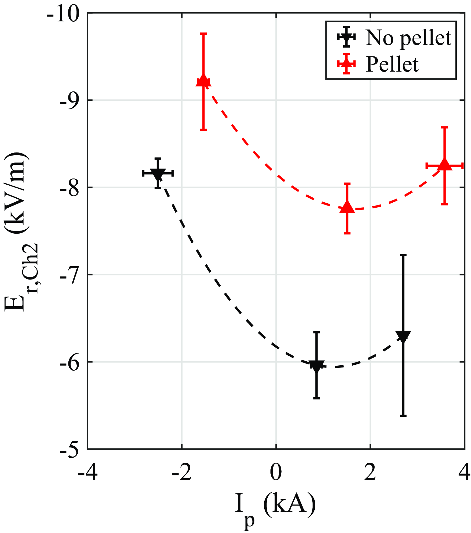
Figure 6. Radial electric field $E_r$ (from Doppler reflectometer channel 2 at $\rho \simeq 0.7$ ) versus $I_{\!p}$ . The dashed lines are meant to guide the eye.

3.5. Magnetohydrodynamic modes

Figure 7 shows Mirnov spectra for three cases with pellet injection and different values of plasma current, $I_{\!p}$ . The ECRH heating is switched off at $t\simeq 1120$ ms, after which NBI heating takes over, activating Alfvén modes. Low frequencies ( $f \lt 100$ kHz) typically correspond to MHD modes, whereas high frequencies ( $f \gt 100$ kHz) typically correspond to Alfvén modes (Jiménez-Gómez et al. 2011). The injection of pellets ( $1170 \leqslant t \leqslant 1180$ ms) leads to strong spectral suppression.

At negative current, the dominant (highest-amplitude) MHD mode frequency prior to the pellet is 34 kHz, at zero current the mode is incoherent and at positive current the dominant mode frequency is 18 kHz. The observed mode frequency can be estimated as $f \simeq mv_\theta /(2\pi r)$ . Thus, a lower mode frequency is an indication, but no evidence, of a lower value of $m$ . To properly identify the modes, we apply the analysis method described in § 2.5.

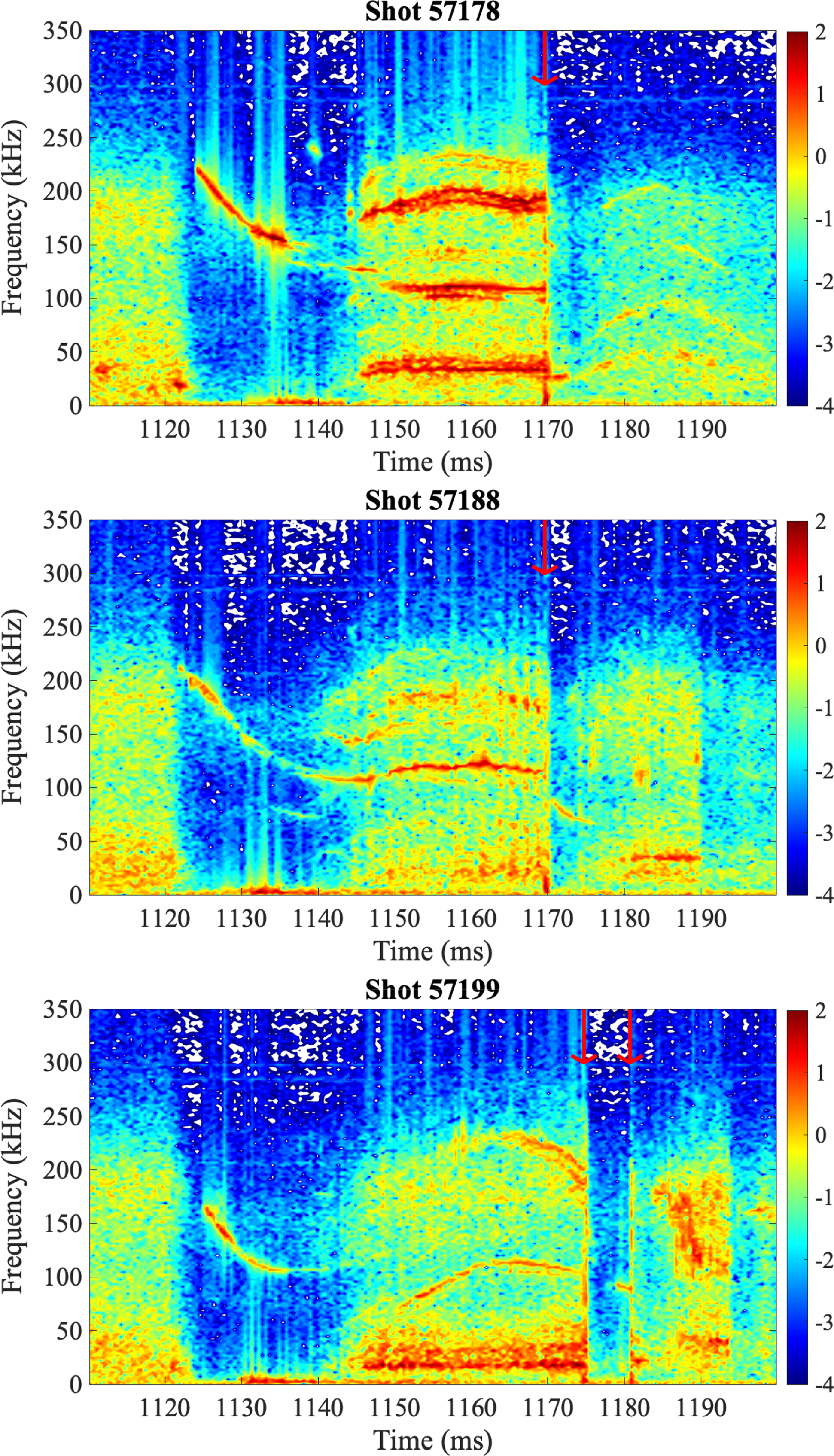
Figure 7. Mirnov spectra for three discharges with (top to bottom) negative, zero and positive current. The ECRH heating phase ends at $t \simeq 1120$ ms, after which NBI heating is switched on. Pellet injection times are signalled with red arrows.

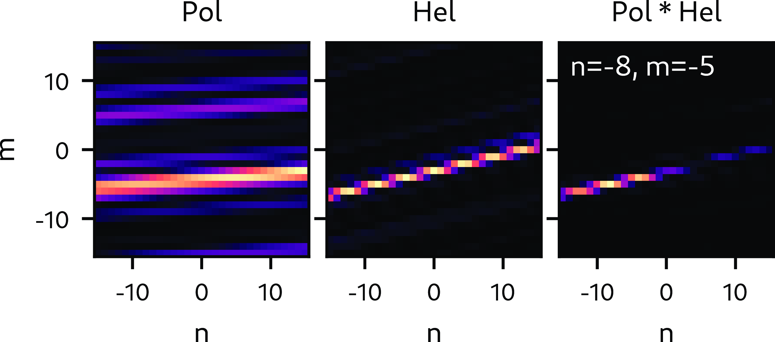
Figure 8. Results of the periodogram analysis for the negative current case (57178) using only the poloidal array (left), the helical array (central) and combining both results (right). The bands that appear in the upper part of the poloidal map are due to signal noise as shown in Pons-Villalonga et al. ( 2025).

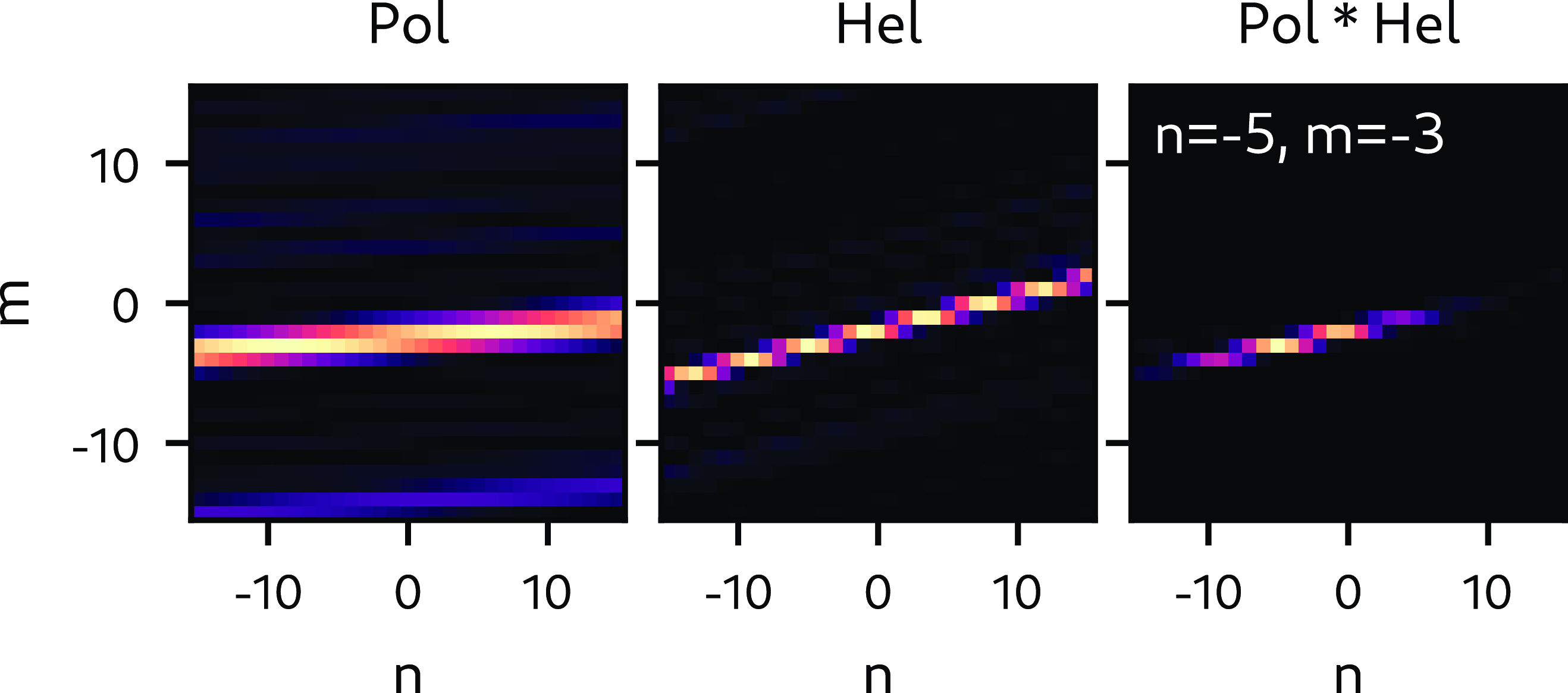
Figure 9. Same as figure 8 but for the negative current case (57195).

Figures 8 and 9 show the results of mode number analysis for discharges 57178 and 57195, corresponding to negative and positive current, respectively. Consistently with the estimates made for the rotational transform, a dominant pair of mode numbers $n=-8$ , $m=-5$ is detected for the negative current case while $n=-5$ and $m=-3$ is found for positive current. The negative sign in both cases arises from the phase convention used in the periodogram analysis, $\varTheta \sim {\rm e}^{{\rm i}(m\theta +n\phi -\omega t)}$ . These findings are consistent with the expectations based on figure 1 (right) regarding dominant modes occurring in the plasma edge and gradient regions.

The radial position of the low-frequency modes can be confirmed from measurements with the HIBP system. One of the two systems, HIBP 2, was operated in scanning mode, in which the sample volume is gradually swept through the plasma from $\rho = -1$ to $\rho = 1$ (negative $\rho$ values referring to the high-field side and positive $\rho$ values to the low-field side of the plasma). The mode location can be determined from the cross-coherence between the scanned measured HIBP plasma potential, $\varPhi$ , and a Mirnov magnetic field pickup coil, as these modes have both an electrostatic and an electromagnetic component.

Recall that the cross-coherence between two signals $x(t)$ and $y(t)$ is defined as

(3.1) \begin{align} \gamma _{xy}(f) = \frac {|\langle \hat x(f) \hat y^*(f)\rangle |}{\sqrt {\langle |\hat x|^2(f)\rangle \langle |\hat y|^2(f)\rangle }}, \end{align}

where $\hat x(f)$ is the Fourier transform of $x(t)$ and the star indicates a complex conjugate. Angular brackets indicate an ‘ensemble average’. In this case, $\gamma _{xy}(f)$ is evaluated for successive time intervals of 0.5 ms, each of which is subdivided into 10 subintervals of 50 μs to evaluate the required Fourier transforms and calculate this ‘ensemble average’.

Figure 10 shows an example result for negative $I_{\!p}$ . The signal $\dot B$ from a Mirnov coil, which includes the 8/5 mode at $f \simeq 33$ kHz visible in the spectrum of $\dot B$ , displays significant bursts of coherence with the oscillations of the HIBP potential (red circles) at this same frequency. By matching the time of the coherence bursts with the calculated location of the HIBP sampling volume (vertical dashed lines), one may deduce that the detected 8/5 mode is located at $0.7 \lt |\rho | \lt 0.8$ . As a side remark, and by the same reasoning, the higher-frequency modes ( $f \gt 100$ kHz) also visible in the spectrum (likely Alfvén modes) are located over a broad radial range in the core plasma. This example result is reproducible over a significant number of discharges.

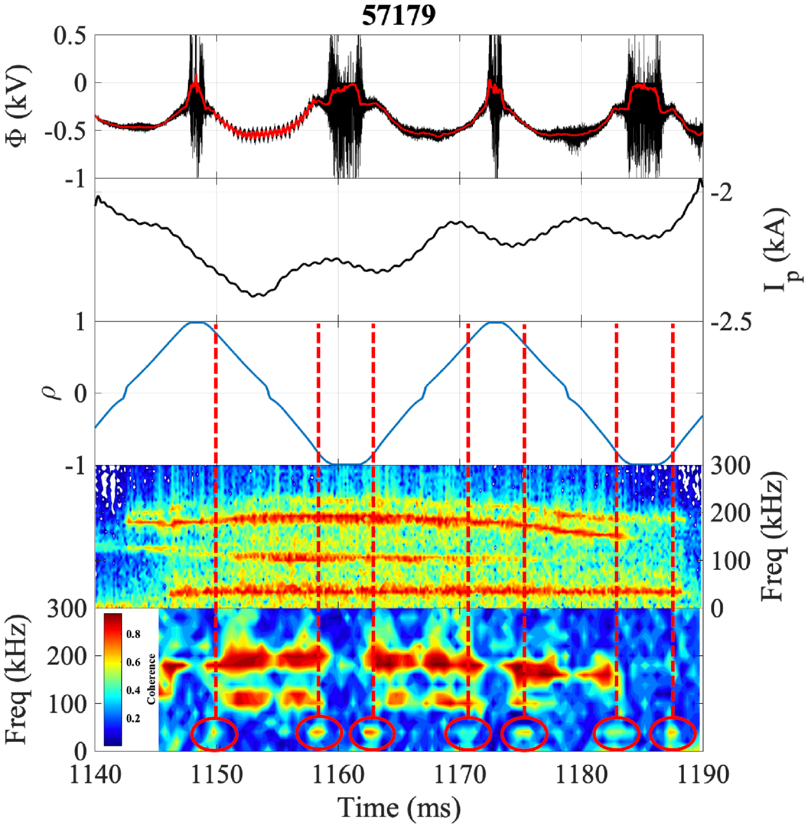
Figure 10. Cross-coherence analysis, discharge 57179, negative $I_{\!p}$ . Top to bottom: measured HIBP plasma potential, $\varPhi$ (kV); measured plasma current, $I_{\!p}$ (kA); approximate normalised radial location of the HIBP sample volume; spectrum of $\dot B$ from a Mirnov coil (a.u., logarithmic colour scale); cross-coherence between $\varPhi$ and $\dot B$ from a Mirnov coil.

Figure 11 shows an example result for positive $I_{\!p}$ , clarifying that the detected 5/3 mode at $f \simeq 40$ kHz is located at $0.7 \lt |\rho | \lt 0.9$ (as indicated by red ellipses and vertical dashed lines). The potential $\varPhi$ shows significant radial structure in the form of a ‘hump’, associated with this low-order mode. Furthermore, strong coherence at the same frequency also occurs in the core plasma region (separately from the edge, as indicated by the green rectangles; corresponding to $|\rho | \lt 0.5$ ), suggesting that for positive current ( $I_{\!p} \gtrsim 2.8$ kA) the rotational transform profile is similar to the curve labelled $I_{\!p} = 2$ kA in figure 1 (left), namely with a minimum at half-radius, so that the 5/3 rational surface occurs twice, in both the plasma edge and core, also in qualitative agreement with figure 1 (right) for positive net plasma currents.

The figure shows that the double-mode occurrence (edge/core) appears for rather high current values, $I_{\!p} \gtrsim 2.8$ kA. However, according to the simple ${\unicode{x0335}\mskip-3.5mu\iota}$ model, (2.1), this situation is expected to occur for lower positive currents, namely $I_{\!p} \simeq 2$ kA (cf. figure 1 (right)). This minor quantitative discrepancy is ascribed to the excessive simplicity of the model: it assumes a fixed current distribution that does not take into account profile shaping effects due to current diffusion.

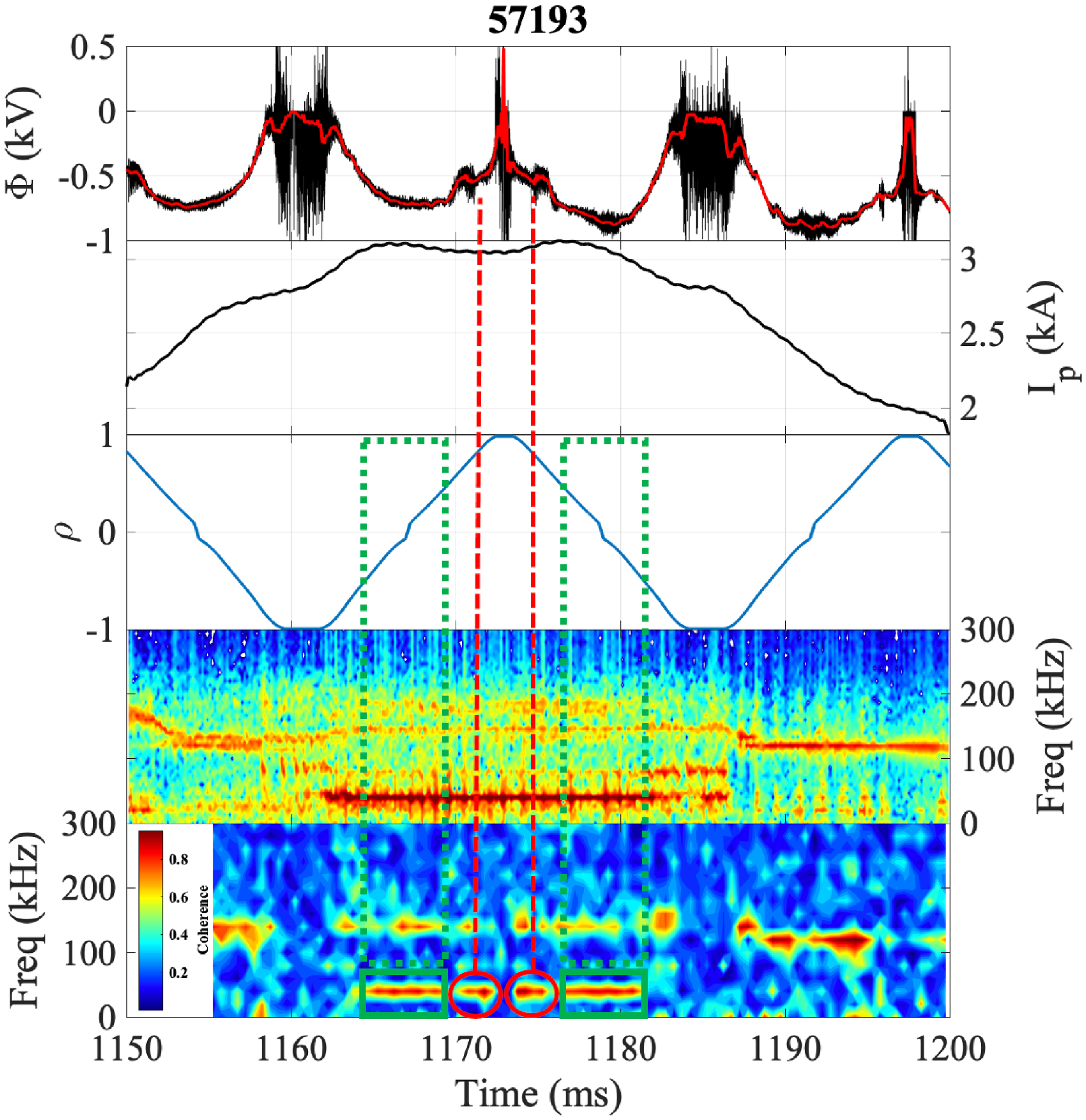
Figure 11. Cross-coherence analysis, discharge 57193, positive $I_{\!p}$ . Same signals as in figure 10. Red circles and dashed lines: high coherence observed in the plasma edge. Green rectangles: high coherence observed in the plasma core, at the same frequency.

4. Numerical results

Turbulence calculations were made using a resistive MHD turbulence model (see § 2.8). We initiate the calculations applying a rotational transform profile corresponding to the magnetic configuration 100_48_65 of TJ-II. The sharp increase in density induced by the pellet is modelled by introducing a density pulse. To achieve this, a very short ( $\Delta t = 0.002 \tau _R$ ) Gaussian pulse, centred at the origin, is added to the source term of the density equation. This method enables us to replicate a rapid density rise of similar magnitude to that observed in the experiment. Immediately after this short interval of time, we also modify the rotational transform profile to take the induced current into account. This modification is implemented using the expression of (2.1). The flux-averaged profiles evolve self-consistently during the turbulence simulation.

To interpret the experimental results discussed above, we have considered several different values for the applied current. Figure 12 (left) shows the rotational transform profile for these cases. The current range is similar to the experiment, namely $-2 \lt I_{\!p} \lt 3$ kA. The modification of the rotational transform is significant in this range. For these cases, the resonant surfaces that play a critical role in modifying the confinement are 3/2, 8/5 and 5/3.

Figure 12 (right) presents the resulting simulated density profiles, after a time interval of $0.14\tau _R$ following the application of the density pulse. In this figure, the density is normalised to the equilibrium density at the magnetic axis before pellet injection, denoted as $n_{eq}(0)$ , thus showing the density increase produced by the density pulse. The depicted profiles correspond to self-consistent steady-state conditions of the turbulence simulation.

To highlight the systematic variation of the density profile with $I_{\!p}$ , figure 13 (left) shows the mean density gradient in the radial range $0.5 \leqslant \rho \leqslant 0.8$ . Note that the variation is qualitatively similar to what was observed in the experiment, cf. figure 5 (left), namely a U-shaped curve with a minimum at small positive values of $I_{\!p}$ .

A useful parameter to measure the improvement of the turbulent transport is the effective particle confinement time, $\tau_{\textrm{eff}}$ , which only takes the turbulent fluxes into account, defined as

(4.1) \begin{equation} \tau_{\textrm{eff}}(r) = \frac {\int _0^r{x n_e(x){\rm d}x}}{\langle r \varGamma (n_e(r))\rangle }. \end{equation}

The formula for the radial particle flux, $\varGamma$ , is derived from the density evolution equation and includes two main components: the product of density with the fluctuating radial $E\times B$ velocity and a term related to the fluctuating magnetic field (see equation (10) in García et al. (2001)). In the examples presented here, the contribution from the latter term is minimal.

Figure 13 (right) shows the effective particle confinement time as a function of the current. Ignoring the point at very high current ( $I_{\!p} = 3$ kA), one again observes the qualitative similarity to the experimental results shown in figure 5 (right), in particular the U shape and the fact that the minimum occurs near $I_{\!p} \simeq 1$ kA. The increasing trend of $\tau_{\textrm{eff}}$ for $I_{\!p} \gt 0.7$ kA is interrupted by the point at $I_{\!p}=3$ kA. The cause for this drop is the loss of the 5/3 rational, which is no longer inside the plasma at this high value of $I_{\!p}$ (cf. figure 12 (left)).

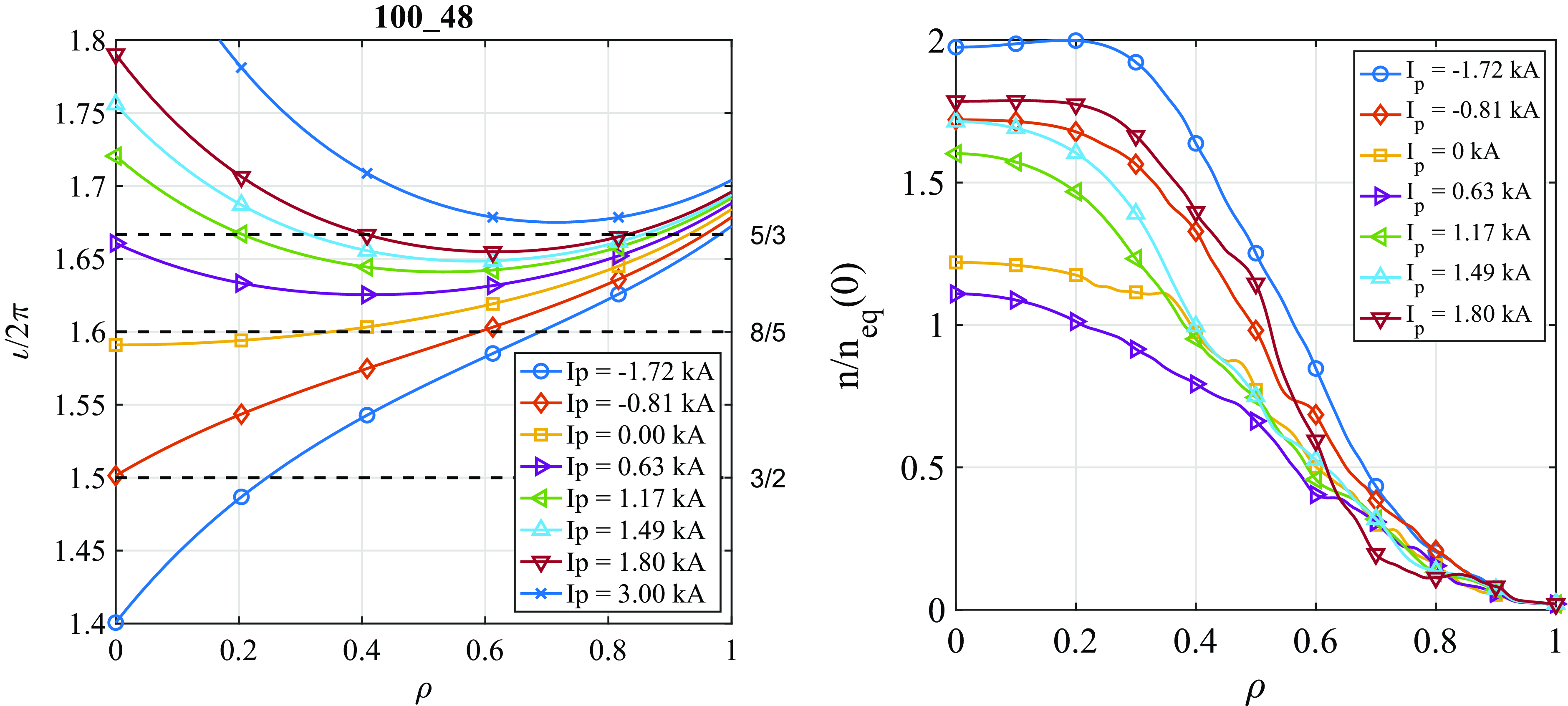
Figure 12. Left: rotational transform profiles used in the turbulence model. Important low-order rational values are indicted by horizontal dashed lines. Right: steady-state density profiles obtained self-consistently from the model.

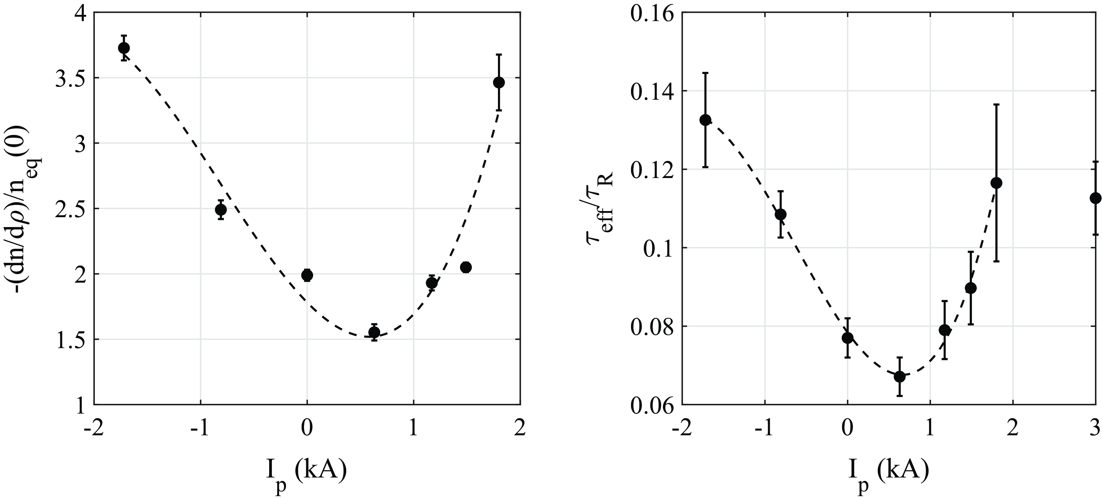
Figure 13. Left: mean density gradient in the radial range $0.5 \leqslant \rho \leqslant 0.8$ . Right: effective turbulence confinement times $\tau_{\textrm{eff}}$ obtained from the model (equation (4.1)). The dashed lines are meant to guide the eye.

In this 100_48_65 configuration, a double 5/3 singular surface may occur at specific positive values of the current, here for the cases $I_{\!p} = 1.17,\ 1.49,\ 1.8$ kA. In the radial interval between the two 5/3 surfaces, the set of rationals $n/m$ is such that only high-order rationals exist. This is illustrated in figure 14. Since higher-order rationals produce a smaller amplitude of fluctuations, if they are triggered at all given the driving gradients, this means that the level of MHD turbulence decreases in this radial region. Due to this reduction of turbulence, the density gradient will subsequently increase until the turbulence reaches the same level as before (a consequence of self-organisation: the turbulent transport needs to self-regulate until a new steady-state situation is reached). In this new situation, the amplitude of the fluctuations corresponding to the 5/3 rationals is higher than before the current change, due to the increased gradients, and so are the barriers that they generate. The final result of this complex, self-organised situation is an improved confinement state.

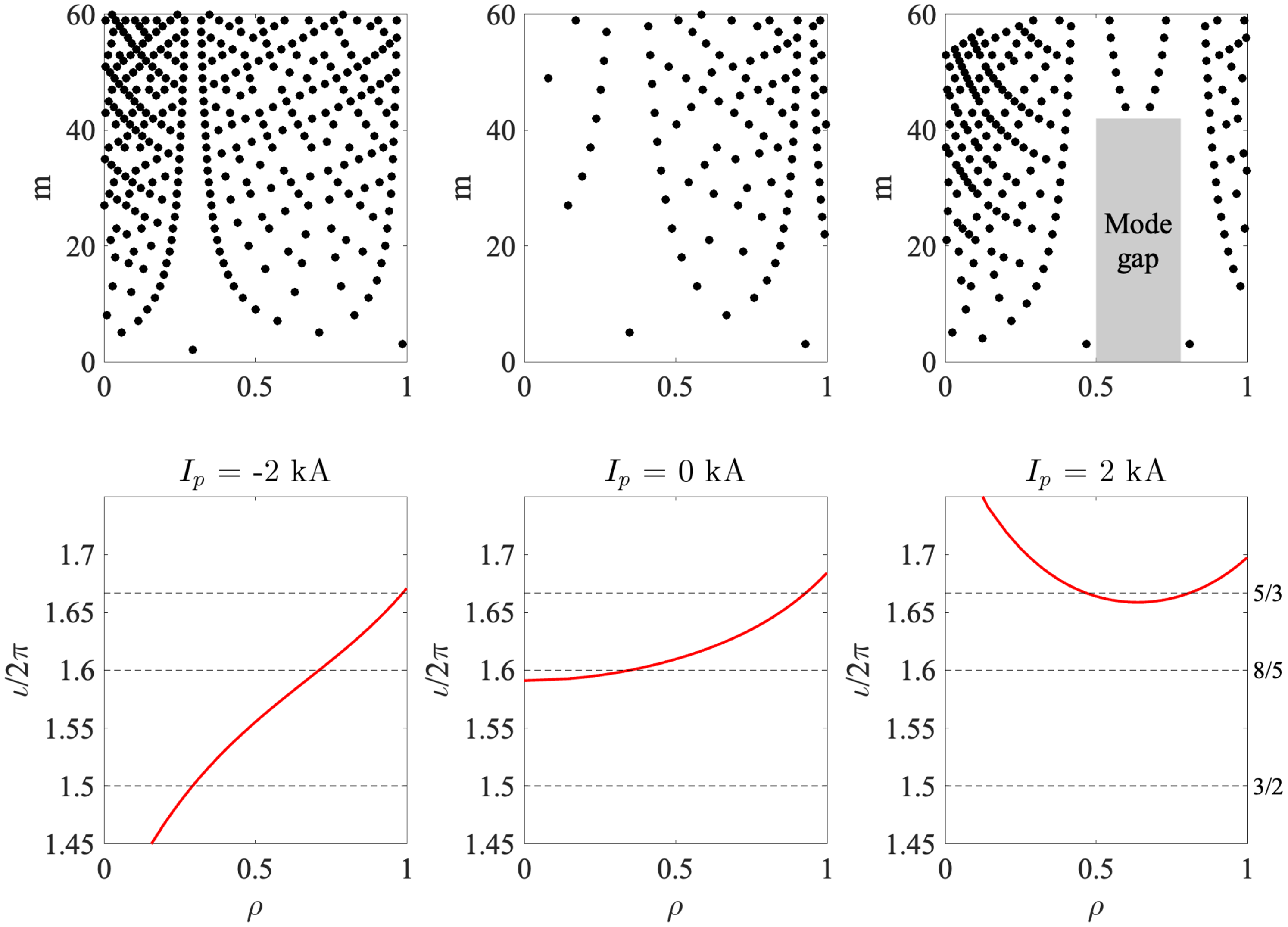
Figure 14. The top panels show the $m$ values of the MHD resonances $n/m$ according to the rotational transform model of (2.1), shown in the bottom panels, for $I_{\!p} = -2,\ 0,\ 2$ kA. When the rotational transform profile is ‘hollow’ and its minimum is close to a low-order rational (right two panels), a broad zone is created where no low-order resonances exist (indicated by a grey area), in this case roughly in the density gradient region.

For the negative current cases, the mechanism of confinement improvement is different. In this case, the 3/2 surface enters the plasma (cf. figure 1), reinforcing the coupling between the 8/5 and 5/3 modes (such long-range coupling was studied in van Milligen et al. (2016), for a different case). This coupling enhances the fluctuation levels associated with these low-order rationals, intensifying the corresponding transport barriers.

These different ways in which the change of rotational transform affects the effective confinement can be identified by looking at the effective confinement as a function of the radius (figure 15 (left)). In the case of positive $I_{\!p}$ , a clear peak of $\tau_{\textrm{eff}}$ is seen at $\rho \simeq 0.5$ , close to the innermost of the two 5/3 rational surfaces. This peak constitutes an effective local transport barrier (cf. Ichiguchi & Carreras 2011). No peak is seen near the outermost 5/3 rational surface at $\rho \simeq 0.75$ , since the driving gradient is quite low at that location (cf. figure 12 (right)). However, a second peak appears at $\rho \simeq 0.6$ , near the minimum of the hollow rotational transform profile (i.e. in the ‘mode gap’). In the case of negative $I_{\!p}$ , $\tau_{\textrm{eff}}$ is enhanced broadly but shows a sharp peak below $\rho \simeq 0.4$ , near the 3/2 rational surface.

The poloidal velocity profile, shown in figure 15 (right), is also of interest. All cases show a dip in the edge region (around $\rho \simeq 0.8$ ). In the case of positive $I_{\!p}$ , a very marked additional dip is seen around $\rho \simeq 0.55$ , related to the second radial occurrence of the 5/3 rational surface. Rather steep sections of $V_\theta (\rho )$ (i.e. high-velocity shear) are related to the mentioned two peaks of $\tau_{\textrm{eff}}$ . In the case of negative $I_{\!p}$ , the velocity profile has significantly more radial structure than in the case of $I_{\!p}= 0$ kA, in part associated with the 8/5 rational and related to additional improved confinement, as commented above.

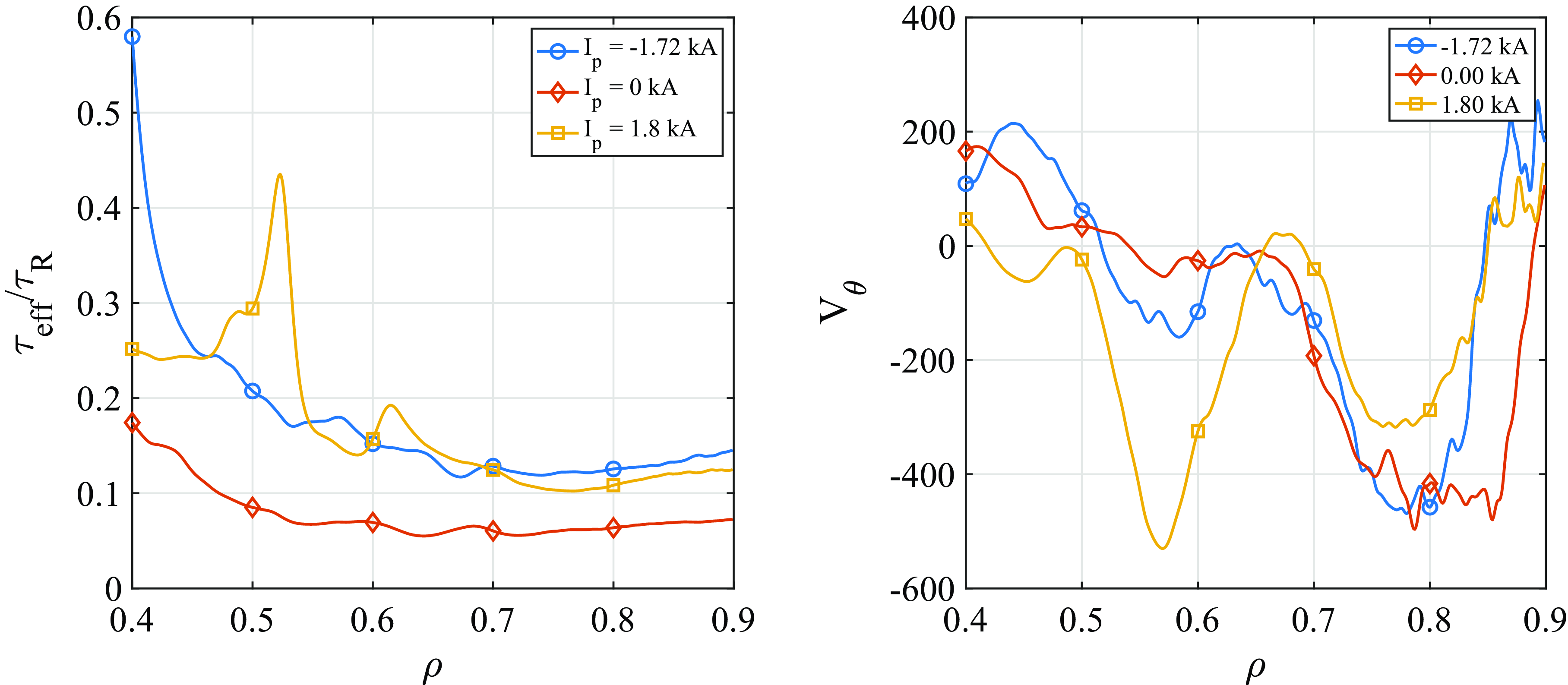
Figure 15. Effective turbulence confinement times (left) and mean poloidal velocities (right) versus normalised radius.

5. Discussion

The main motivation of this study is to try to understand the mechanism behind the variation of the plasma energy content $W_{\textrm{th}}$ with small changes of the rotational transform in low-magnetic-shear configurations. This effect has been reported in earlier experimental studies for several devices, including TJ-II (Hirsch et al. 2008; Ascasíbar et al. 2008; Estrada et al. 2010).

Neoclassical transport theory does not appear to provide an immediate explanation for these observations. Firstly, this theory predicts much lower transport levels than those actually observed in this type of discharge, by a factor of $2{-}3$ (García-Cortés et al. 2023), so that its action is subdominant. Secondly, this theory does not predict any significant change of confinement if the rotational transform is varied only slightly, all else being equal (Velasco & Castejón 2011).

Here, this issue is addressed both experimentally and using a resistive MHD turbulence model at the TJ-II stellarator. The vacuum configuration studied is the one labelled 100_48_65, and NBI-heated plasmas with pellet injection are considered, often displaying enhanced confinement (García-Cortés et al. 2023). Experimentally, the rotational transform profile is modified by controlling the net plasma current $I_{\!p}$ using external coils (see §§ 2.1 and 2.2). Target current values were set at $I_{\!p} = -2,\ 0,\ 2$ kA. Reproducibility of the experimental results was good. For $I_{\!p} \simeq -2$ and $I_{\!p} \simeq 2$ kA, confinement was significantly improved with respect to the case $I_{\!p} \simeq 0$ (figure 5). Results from the turbulence model (figure 13) are qualitatively consistent with the experimental results.

For these low-magnetic-shear configurations, the very low-mode-number rationals are spatially separated from the other low-order rationals and do not always contribute to the turbulence. But even if they do not, low-order modes may create vortices that trap particles and generate sheared flows associated with transport barriers. In the present experiments, a mode number analysis of the toroidal and poloidal sets of Mirnov pickup coils showed that specific modes were dominant in the different cases, namely $n/m = 8/5$ for negative $I_{\!p}$ and 5/3 for positive $I_{\!p}$ . The fact that confinement improves when these modes are present indicates that the rotating modes do not lead to the formation of large islands.

Considering the different values of $I_{\!p}$ , we find:

1. (i) With positive $I_{\!p} \simeq 2$ kA, the low-order rational 5/3 enters the gradient region (see figure 1 (right)). The enhanced confinement at such positive $I_{\!p}$ values is associated with the predicted simultaneous existence of the 5/3 rational surface at two radial positions (see figure 1 (left)). This possible double occurrence of a major low-order rational finds experimental support from the coherence analysis between signals from the radially scanned HIBP system and a Mirnov pickup coil (figure 11). In this situation, the zone between the two rational surfaces is free from low-order rationals, as shown in figure 14, leading to low turbulence levels and enhanced gradients. In the simulation, the formation of a transport barrier at the innermost occurrence of this double rational, as well as near the location of the rotational transform profile minimum, could be visualised clearly on the basis of the radial profile of the effective turbulence confinement time, $\tau_{\textrm{eff}}$ (figure 15).

2. (ii) With negative $I_{\!p} \simeq -2$ kA, the low-order rational 8/5 enters the gradient region. The enhanced confinement at such negative $I_{\!p}$ values is related to enhanced fluctuation levels at the low-order rational surfaces, likely involving radial coupling occurring between the 3/2, 8/5 and 5/3 rationals, leading to enhanced transport barriers. Such long-range coupling effects were studied in earlier work (van Milligen et al. 2016).

3. (iii) With small positive $I_{\!p} \simeq 0{-}1$ kA, no low-order rationals (such as the 5/3 and 8/5 rationals) are present in the gradient region, and this presumably leads to lower-amplitude MHD-type fluctuations. On the other hand, higher-order rationals are not suppressed (as in the case of the double 5/3 above), which is consistent with the fact that the detected low-frequency magnetic activity is incoherent in this case (cf. figure 7). A lower MHD turbulence amplitude is associated with less intense zonal flow generation and associated transport barriers, and the lack of suppression of turbulence might explain the reduced plasma energy content values in this situation.

6. Conclusions

In this work, we show how the confinement quality of the TJ-II stellarator depends on the rotational transform profile, which in these experiments is controlled by the net plasma current, $I_{\!p}$ . By changing $I_{\!p}$ , significant variations of the edge density gradient (by a factor of 2) and the plasma energy content ( $20\,\%{-}30\,\%$ ) can be achieved. This phenomenon was confirmed by resistive MHD turbulence calculations, which exhibit a variation of profile gradients and the effective turbulence confinement time, as a function of the rotational transform profile, that is qualitatively similar to the experimental variation.

The experimental and turbulence modelling observations suggest that when low-order rational surfaces are placed roughly at the foot of the density gradient region, energy confinement may be enhanced. The location of other low-order surfaces may also play an important role, by enhancing zonal flows through nonlinear coupling with the rational surface placed at the foot of the density gradient.

Making use of the broad array of diagnostics available at TJ-II, this work shows how this hypothesis is borne out experimentally in terms of enhanced plasma energy content, enhanced density gradients in the edge and enhanced values of the edge radial electric field $E_r$ as a function of the plasma current $I_{\!p}$ . Various MHD mode analyses confirmed the expected modification of the rotational transform profile associated with $I_{\!p}$ in significant detail.

In summary, the observed variation of confinement as a function of $I_{\!p}$ could be understood in terms of transport barriers associated with low-order rational surfaces in the density gradient region, while the radial location of these rational surfaces is modified when $I_{\!p}$ is varied. This mechanism thus provides an external control knob to manipulate the confinement quality of low-shear stellarators and perhaps other magnetic confinement devices.