Input misallocation and productivity dynamics

Abstract

This paper builds on Hsieh and Klenow’s (2009) model to offer a refined analysis of how input misallocations impact aggregate total factor productivity (TFP). We enhance the original model by relaxing the assumption of uniform input prices and adopting an econometric approach to estimate parameters using firm-level data. Estimation of model parameters and allocation efficiency is based on the system of input demand and the production function. We use an indirect inference approach to estimate the system to avoid maximum likelihood estimation, which often faces convergence issues, when there are numerous constraints. We demonstrate our model using the US firm-level manufacturing panel data from 1975 to 2010. Our final sample contains 55,518 observations. We divide the manufacturing industry into seven major categories. Our findings indicate that between 1975 and 2010, the average productivity growth rate was 2.8% but could have reached 3.2% without misallocation, highlighting the substantial gains possible through better resource allocation.

1. Introduction

Input misallocation refers to the inefficient distribution of resources, such as labor, capital, and materials, between firms or sectors within an economy. When inputs are not allocated optimally, firms that could use them more productively may receive fewer resources, while less efficient firms may receive more than they can effectively use. This misallocation can result from market distortions that obstruct the free flow of resources to the appropriate firms. Consequently, it leads to significant losses in overall productivity and economic growth. From a macro perspective, understanding the dynamics of input misallocation is crucial because it sheds light on how distortions, such as policy interventions, market imperfections, or institutional constraints, can impact aggregate productivity. By analyzing these dynamics, researchers and policymakers can identify strategies to improve resource allocation, improve productivity, and stimulate economic growth.

In this paper, we build upon the foundational work of Hsieh and Klenow (2009) but dig deeper into the effects of resource misallocation on aggregate total factor productivity (TFP) and revenue loss across firms. The central contribution of our research lies in the refinement of the structural model proposed by Hsieh and Klenow (HK), which allows us to provide a more precise and detailed estimation of allocation efficiency (AE), particularly when assessed through the lens of revenue output.

Although our model is grounded in the HK framework, it introduces several enhancements that address limitations in the original model. One of the key improvements is our departure from the assumption of uniform input prices across firms, which is unrealistic. By incorporating heterogeneous input prices, our model seeks to offer a more precise estimation of input misallocation and productivity dynamics. Relying on uniform input prices would overlook these essential cross-group variations. Our model includes three inputs, capital (K), labor (L), and materials (M), allowing us to capture the complexities of firm-level production processes and the inefficiencies in the allocation of these three inputs. The three-input production model is standard in structural productivity models such as Olley and Pakes (1996) and many others that followed them. From an empirical model specification standpoint, incorporating $ K$ , $ L$ , and $ M$ as key variables in the production function aligns with standard practices in firm-level analyses. Unlike many macroeconomic models that consider only $ K$ and $ L$ , the inclusion of $ M$ addresses potential issues related to omitted variable bias. By incorporating materials ( $ M$ ), our model provides a more accurate representation of production processes and enhances the reliability of the results. This inclusion captures a more comprehensive production structure, allowing us to account for additional sources of misallocation that influence productivity dynamics.

In addition to this, we diverge from the conventional calibration methods commonly employed in the macro literature. Almost all existing papers use calibration, and these papers set some structural parameters a priori, instead of estimating them. However, the parameters used in the calibration can lead to differences in the prediction and analysis of subsequent results. Take the output substitution elasticity $\sigma _{s}$ in HK as an example. Different values of $\sigma _{s}$ make the predictions of the hypothetical TFP gains of China and India significantly different. Whether the difference in the prediction results is significant is determined based on robustness checks. Calibration often relies on predefined assumptions that may not hold in all contexts, potentially leading to biased or inaccurate results. To overcome this, we adopt an econometric approach to estimate the model parameters; it is novel and has not been used before in the macro literature. Our process begins by deriving the input demand function from each firm’s optimization problem. This derivation generates the input demand functions for the three endogenous inputs, while input prices remain exogenous. We then employ firm-level data to estimate structural parameters across different manufacturing subsectors, which allows us to account for the heterogeneity in production technologies that exist between subsectors. This approach allows us to obtain more accurate estimates of firm-specific misallocations and the marginal revenue product (MRP) of inputs, independent of variations in TFP.

The aggregation of these firm-level estimates enables us to analyze the effects of misallocation at both the sectoral and industry levels. Our findings reveal that during the period 1975 to 2010, the average productivity growth rate, as measured by revenue-based total factor productivity (TFPR), was approximately 2.8%. However, through counterfactual analysis, we show that this growth rate could have been as high as 3.2% if resource misallocation between firms had been eliminated. This significant difference demonstrates the substantial impact that misallocation can have on overall productivity and emphasizes the potential economic gains that could be achieved through improved resource allocation.

Estimation of model parameters and AE is based on the system of input demand and the production function. The coefficients in the demand system are restricted functions of the model parameters, which poses challenges for convergence when applying maximum likelihood estimation (MLE). These challenges are aggravated by the complexity introduced by numerous constraints. To address this issue, we employ an indirect inference procedure. This approach allows us to bypass some of the difficulties associated with direct MLE. Because our model does not include exogenous variables, such as policy variables or firm-specific characteristics that could affect resource allocation or TFPR, the scope of our discussion of the empirical results is limited. Therefore, our discussion focuses mainly on the estimation methods, the prediction of the estimation results, and how our estimation method differs from existing methods. However, it is easy to generalize our model to explore more deeply the factors influencing resource allocation or policy impact. For instance, these exogenous factors can be incorporated into our model by including exogenous factors in the setting of the dynamics of TFPR in order to conduct more in-depth empirical analysis.

The main contributions of the paper are as follows. First, our model extends the HK framework by incorporating heterogeneity in input prices across firms. This extension acknowledges that firms do not operate under uniform conditions. Second, we include three distinct inputs, capital, labor, and materials, to better capture the complexities of production processes at the firm level and the resulting inefficiencies that may arise from misallocation. Third, we employ a state-of-the-art econometric approach to estimate the model parameters based on the system of input demand and the production function. We use an indirect inference procedure instead of the classical maximum likelihood method since there are numerous constraints. Conducting counterfactual analysis using our proposed analytical framework is relatively straightforward and easy to implement.

2. Relevant literature

The Hsieh and Klenow (2009) model has been instrumental in shaping our understanding of how resource misallocation affects aggregate productivity. By quantifying productivity losses due to misallocation, particularly in China and India compared to the United States, the model has highlighted significant inefficiencies in the allocation of capital and labor within industries. Here, we consider some extensions of the HK model, evaluating their contributions to the literature and their implications for policy and future research. The purpose is not to provide a full review of the literature.

Bartelsman et al. (2013) introduce a dynamic perspective by incorporating firm turnover (entry and exit) into the analysis. It reflects the reality that inefficient firms exit the market while more productive ones enter, thus affecting aggregate productivity. These authors argue that dynamic selection plays a key role in explaining productivity differences across countries. However, they assume that the selection process is purely efficiency-driven, potentially overlooking other factors like market power or regulatory barriers that might affect firm turnover.

David et al. (2016) introduce information frictions, where firms may not fully know their productivity and therefore may not allocate resources optimally. This extension is significant because it draws attention to the role of information asymmetries in perpetuating misallocation. However, it abstracts away from how firms might endogenously invest in acquiring better information and how markets and institutions could evolve to reduce these frictions over time.

Bento and Restuccia (2017) extend the HK model by examining the impact of size-dependent policies, such as subsidies, taxes, and regulations, on resource misallocation. Bento and Restuccia argue that policies that disproportionately affect firms based on their size can distort resource allocation, thereby reducing overall productivity. They primarily focuse on policy distortions in isolation and do not fully explore how these policies interact with other forms of distortion, such as financial friction and market power.

Asker, et al. (2014) introduce dynamic inputs and adjustment costs into the HK framework. This extension accounts for the reality that adjusting inputs, such as labor and capital, often involves costs, leading to persistent misallocation. Although this model more accurately reflects the challenges firms face in optimizing resource use, it could be criticized for its complexity, which could limit its practical application, especially in policy-making contexts where simpler models are often preferred.

Gopinath et al. (2017) apply the HK model to the specific context of Southern Europe, focusing on the period before and after the financial crisis. This regional application shows how financial frictions and firm-specific shocks can exacerbate capital misallocation, particularly during economic downturns. The findings, while relevant to Southern Europe, might not be directly applicable to other regions with different institutional or economic structures.

Uras and Wang (2024) examine how resource misallocation impacts productivity by influencing firms’ adoption of efficient production techniques. Thus, their paper extends traditional models by allowing production techniques to be endogenous, meaning that firms can adjust their production methods based on the resources available to them and the level of misallocation. This approach provides a more dynamic view of how misallocation affects productivity and development. They find that misallocation affects productivity both directly and indirectly.

Our focus, distinct from the models mentioned above, is primarily on the input allocation at the firm level, where misallocation occurs. We analyze the revenue loss resulting from misallocation at the firm level, which is then used to assess the revenue loss at more aggregate levels. between firms or across industries.

3. The model

In this section, we introduce the economic environment and show how the aggregate output reflects the cross-sector misallocation.

3.1. Aggregate economy and intermediate goods sector

In this framework, the model follows Hsieh and Klenow (2009) and assumes a hierarchical structure. At the top level is the aggregate economy, followed by individual industries, with each industry comprising constituent firms. There is a single final good $Y$ produced/sold in a perfectly competitive final output market. There are $S$ industries and $M_{s}$ number of firms in each of the industries $s,$ where $s=1,\ldots, S$ . Assume that the production technology (aggregator function) at the top can be captured by a Cobb–Douglas function, that is,

(1) \begin{align} Y= {\prod \nolimits _{s=1}^{S}} Y_{s}^{\theta _{s}},\text { } \end{align}

where

(2) \begin{align} {\sum \nolimits _{s=1}^{S}} \theta _{s}=1. \end{align}

Furthermore, let

(3) \begin{align} Y_{s}=\left ( {\sum \nolimits _{i=1}^{M_{s}}} Y_{si}^{\frac {\sigma _{s}-1}{\sigma _{s}}}\right ) ^{\frac {\sigma _{s}}{\sigma _{s}-1}} \end{align}

denote the constant elasticity of substitution (CES) aggregator function of $M_{s}$ differentiated products for industry $s$ . The production technology for each differentiated product (firm technology) is

(4) \begin{align} Y_{si}=A_{si}K_{si}^{\alpha _{s1}}L_{si}^{\alpha _{s2}}M_{si}^{\alpha _{s3}},\text { } \end{align}

where the capital, labor, and material shares ( $\alpha _{s1},\alpha _{s2},\alpha _{s3}$ ) are bounded between 0 and 1 and allowed to vary by industry. Moreover, $\alpha _{s1}+\alpha _{s2}+\alpha _{s3}=1$ satisfies the constant return to scale (CRTS) production technology. The output elasticities $\alpha _{s1},\alpha _{s2}$ , and $\alpha _{s3}$ are sector-specific, but time-invariant and common across firms within a sector.

Let $P_{s}$ denote the price of industry output $Y_{s}.$ The final good producer maximizes

(5) \begin{align} \underset {Y_{1},\ldots, Y_{S}}{\max }PY- {\sum \nolimits _{i=1}^{S}} P_{s}Y_{s}. \end{align}

The FOC from profit maximization of the final goods subject to (1) and (2) gives

(6) \begin{align} P_{s}Y_{s}=\theta _{s}PY, \end{align}

which suggests the price of the final good is

(7) \begin{align} P= {\prod \nolimits _{s=1}^{S}} \left ( \frac {P_{s}}{\theta _{s}}\right ) ^{\theta _{s}}. \end{align}

This implies that $PY = \prod \nolimits _{s=1}^{S} \left ( \frac {P_{s} Y_s}{\theta _{s}}\right )$ . These relate the final good price and revenue to industry prices and outputs.

Let $P_{si}$ denote the price of differentiated product $Y_{si}$ . Given that the aggregate of intermediate goods of the industry $Y_{s}$ follows the CES assumption in (3), the demand for the differentiated output $Y_{si}$ can be derived by maximizing the industry’s profit function

(8) \begin{align} \underset {Y_{s1},\ldots, Y_{sMs}}{\max }\pi _{s}=P_{s}Y_{s}-{\sum \nolimits _{i=1}^{M_{s}}}P_{si}Y_{si}. \end{align}

The FOC suggests

(9) \begin{align} P_{s}Y_{s}^{\frac {1}{\sigma _{s}}}Y_{si}^{\frac {\sigma _{s}-1}{\sigma _{s}}}=P_{si}Y_{si}. \end{align}

Thus, the output of firm $i$ of industry $s$ is

(10) \begin{align} Y_{si}=\left ( \frac {P_{s}}{P_{si}}\right ) ^{\sigma _{s}}Y_{s}. \end{align}

3.2. Firm-level economy: TFPR and TFPQ

There are three input factors (capital, labor, and materials) for producing the intermediate goods. Let the prices of capital, labor and materials be $W_{Ksi},W_{Lsi}$ , and $W_{Msi}$ . Because of misallocation, prices are distorted. Without any misallocations or distortions in the input prices, the first-order conditions (FOCs) of cost minimization of firm $i$ in industry $s$ are ¹

\begin{equation*} \frac {{W_{Ksi}}K_{si}}{W_{Lsi}L_{si}}=\frac {\alpha _{s1}}{\alpha _{s2}}\text { and }\frac {W_{Msi}M_{si}}{W_{Lsi}L_{si}}=\frac {\alpha _{s3}}{\alpha _{s2}}. \end{equation*}

We introduce misallocation in the above FOCs (Schmidt and Lovell (1979)) by writing them as:

\begin{equation*} \frac {W_{Ksi}K_{si}}{W_{Lsi}L_{si}}e^{\zeta _{Ksi}}=\frac {\alpha _{s1}}{\alpha _{s2}}\text { and }\frac {W_{Msi}M_{si}}{W_{Lsi}L_{si}}e^{\zeta _{Msi}}=\frac {\alpha _{s3}}{\alpha _{s2}}, \end{equation*}

where $\zeta _{Ksi}$ and $\zeta _{Msi}$ are the misallocation terms for the input pairs $\left ( K,L\right )$ and $\left ( M,L\right )$ . $\zeta _{Ksi}$ and $\zeta _{Msi}$ can take positive or negative values. ² For notational simplicity, we let $\lambda _{Ksi}=e^{\zeta _{Ksi}}$ and $\lambda _{Msi}=e^{\zeta _{Msi}}.$ Thus, the misallocation-adjusted (shadow) prices of capital and materials are $\lambda _{Ksi}W_{Ksi}$ and $\lambda _{Msi}W_{Msi}$ .

Since firms face competitive output markets, $P_{si}$ is known and the expression for $Y_{si}$ shown in (10) is determined from the optimization problem in (8). Firm $i$ minimizes its cost ³ under the misallocation-adjusted (shadow) prices of capital and materials:

(11) \begin{align} \underset {K_{si},L_{si},M_{si}}{\min }C_{si} & =\lambda _{Ksi}W_{Ksi}K_{si}+W_{Lsi}L_{si}+\lambda _{Msi}W_{Msi}M_{si} \nonumber\\[3pt] \text {s.t. }Y_{si} & =A_{si}K_{si}^{\alpha _{s1}}L_{si}^{\alpha _{s2}}M_{si}^{\alpha _{s3}}. \end{align}

The FOCs are

(12) \begin{align} K_{si}=\frac {\alpha _{s1}}{\alpha _{s2}}\frac {W_{Lsi}}{\lambda _{Ksi}W_{Ksi}}L_{si}, \end{align}

(13) \begin{align} M_{si}=\frac {\alpha _{s3}}{\alpha _{s2}}\frac {W_{Lsi}}{\lambda _{Msi}W_{Msi}}L_{si}, \end{align}

and

(14) \begin{align} L_{si}=\frac {\alpha _{s2}}{A_{si}}\left ( \frac {\lambda _{Ksi}W_{Ksi}}{\alpha _{s1}}\right ) ^{\alpha _{s1}}\left ( \frac {W_{Lsi}}{\alpha _{s2}}\right ) ^{\alpha _{s2}}\left ( \frac {\lambda _{Msi}W_{Msi}}{\alpha _{s3}}\right ) ^{\alpha _{s3}}\frac {Y_{si}}{W_{Lsi}}. \end{align}

Furthermore, if there is no misallocation, then $\lambda _{Ksi}=\lambda _{Msi}=1$ and then (12) and (13) degenerate to the standard FOCs from cost minimization problem.

Note that the maximization problem of the industry $s$ in (8) and its FOC in (9) imply that the MRPs of the three inputs are

(15a) \begin{align} MRPK_{si} & =\alpha _{s1}\frac {\sigma _{s}-1}{\sigma _{s}}\frac {P_{si}Y_{si}}{K_{si}} \\[-8pt] \nonumber \end{align}

(15b) \begin{align} MRPL_{si} & =\alpha _{s2}\frac {\sigma _{s}-1}{\sigma _{s}}\frac {P_{si}Y_{si}}{L_{si}} \\[-8pt] \nonumber \end{align}

(15c) \begin{align} MRPM_{si} & =\alpha _{s3}\frac {\sigma _{s}-1}{\sigma _{s}}\frac {P_{si}Y_{si}}{M_{si}}. \\[6pt] \nonumber \end{align}

The marginal revenue of capital is proportional to the revenue-capital ratio. Similar properties hold for the marginal revenues of labor and materials. Moreover, the producer $i^{\prime }$ s optimization behavior should satisfy that the marginal revenue of an input equals the marginal cost of the input, that is,

(16a) \begin{align} \alpha _{s1}\frac {\sigma _{s}-1}{\sigma _{s}}\frac {P_{si}Y_{si}}{K_{si}} & =\lambda _{Ksi}W_{Ksi} \\[-8pt] \nonumber \end{align}

(16b) \begin{align} \alpha _{s2}\frac {\sigma _{s}-1}{\sigma _{s}}\frac {P_{si}Y_{si}}{L_{si}} & =W_{Lsi} \\[-8pt] \nonumber \end{align}

(16c) \begin{align} \alpha _{s3}\frac {\sigma _{s}-1}{\sigma _{s}}\frac {P_{si}Y_{si}}{M_{si}} & =\lambda _{Msi}W_{Msi}. \\[6pt] \nonumber \end{align}

Foster et al. (2008) stress the distinction between physical productivity (TFPQ) and revenue productivity (TFPR) because when industry deflators are used, differences in firm-specific prices show up in the customary measure of plant TFP. Therefore, similar to HK (2009), we define the physical productivity TFPQ as

(17) \begin{align} TFPQ_{si}=A_{si}=\frac {Y_{si}}{K_{si}^{\alpha _{s1}}L_{si}^{\alpha _{s2}}M_{si}^{\alpha _{s3}}} \end{align}

and define the revenue productivity TFPR as

(18) \begin{align} TFPR_{si}=P_{si}A_{si}=\frac {P_{si}Y_{si}}{K_{si}^{\alpha _{s1}}L_{si}^{\alpha _{s2}}M_{si}^{\alpha _{s3}}}. \end{align}

Using (9), one can rewrite $TFPQ_{si}$ as

\begin{equation*} TFPQ_{si}=A_{si}=\frac {\left ( P_{si}Y_{si}\right ) ^{\frac {\sigma _{s}}{\sigma _{s}-1}}}{\kappa _{s}K_{si}^{\alpha _{s1}}L_{si}^{\alpha _{s2}}M_{si}^{\alpha _{s3}}}=\frac {\left ( TFPR_{si}\right ) ^{\frac {\sigma _{s}}{\sigma _{s}-1}}}{\kappa _{s}}\left ( K_{si}^{\alpha _{s1}}L_{si}^{\alpha _{s2}}M_{si}^{\alpha _{s3}}\right ) ^{\frac {1}{\sigma _{s}-1}}, \end{equation*}

where $\kappa _{s}=\left ( P_{s}Y_{s}^{\frac {1}{\sigma _{s}}}\right ) ^{\frac {\sigma _{s}}{\sigma _{s}-1}}$ , which is a sector-specific constant.

Using (16a)–(16c) and (18), the $TFPR_{si}$ can also be represented as

(19) \begin{align} TFPR_{si} & =\frac {\sigma _{s}}{\sigma _{s}-1}\left ( \frac {MRPK_{si}}{\alpha _{s1}}\right ) ^{\alpha _{s1}}\left ( \frac {MRPL_{si}}{\alpha _{s2}}\right ) ^{\alpha _{s2}}\left ( \frac {MRPM_{si}}{\alpha _{s3}}\right ) ^{\alpha _{s3}} \nonumber\\[3pt] & =\frac {\sigma _{s}}{\sigma _{s}-1}\left ( \frac {W_{Ksi}}{\alpha _{s1}}\right ) ^{\alpha _{s1}}\left ( \frac {W_{Lsi}}{\alpha _{s2}}\right ) ^{\alpha _{s2}}\left ( \frac {W_{Msi}}{\alpha _{s3}}\right ) ^{\alpha _{s3}}\lambda _{Ksi}^{\alpha _{s1}}\lambda _{Msi}^{\alpha _{s3}} \nonumber\\[3pt] & =\lambda _{Ksi}^{\alpha _{s1}}\lambda _{Msi}^{\alpha _{s3}}TFPR_{si}^{\ast },\end{align}

where $TFPR_{si}^{\ast }=\frac {\sigma _{s}}{\sigma _{s}-1}\left ( \frac {W_{Ksi}}{\alpha _{s1}}\right ) ^{\alpha _{s1}}\left ( \frac {W_{Lsi}}{\alpha _{s2}}\right ) ^{\alpha _{s2}}\left ( \frac {W_{Msi}}{\alpha _{s3}}\right ) ^{\alpha _{s3}}$ denotes the efficient TFPR when there is no allocation inefficiency, that is, $\lambda _{Ksi}=\lambda _{Msi}=1.$ Misallocation of inputs causes the MRPs of capital and materials to deviate from their respective input prices, $W_{Ksi}$ and $W_{Msi}$ , leading to a discrepancy between the observed $TFPR_{si}$ and its efficient benchmark, $TFPR_{si}^{*}$ .

3.3. Aggregation

To derive the impact of misallocation for the industry as a whole, we use the results from the individual firm in section 3.2. Now we show how the aggregate TFPR reflects cross-sector distortions as well as the individual sectors’ TFPR.

Using (16a)–(16c), the industry-specific aggregate inputs are

(20) \begin{align} K_{s}= {\sum \nolimits _{i=1}^{M_{s}}} K_{si}=\alpha _{s1}\frac {\sigma _{s}-1}{\sigma _{s}} {\sum \nolimits _{i=1}^{M_{s}}} \frac {P_{si}Y_{si}}{\lambda _{Ksi}W_{Ksi}}=\alpha _{s1}\frac {\sigma _{s}-1}{\sigma _{s}}\frac {\theta _{s}PY}{\overline {MRPK}_{s}} \\[-24pt] \nonumber \end{align}

(21) \begin{align} L_{s}= {\sum \nolimits _{i=1}^{M_{s}}} L_{si}=\alpha _{s2}\frac {\sigma _{s}-1}{\sigma _{s}} {\sum \nolimits _{i=1}^{M_{s}}} \frac {P_{si}Y_{si}}{W_{Lsi}}=\alpha _{s2}\frac {\sigma _{s}-1}{\sigma _{s}}\frac {\theta _{s}PY}{\overline {MRPL}_{s}} \\[-24pt] \nonumber \end{align}

(22) \begin{align} M_{s}= {\sum \nolimits _{i=1}^{M_{s}}} M_{si}=\alpha _{s3}\frac {\sigma _{s}-1}{\sigma _{s}} {\sum \nolimits _{i=1}^{M_{s}}} \frac {P_{si}Y_{si}}{\lambda _{Ksi}W_{Msi}}=\alpha _{s3}\frac {\sigma _{s}-1}{\sigma _{s}}\frac {\theta _{s}PY}{\overline {MRPM}_{s}}. \\[6pt] \nonumber \end{align}

where

(23) \begin{align} \overline {MRPK}_{s} & =\left ({\sum \nolimits _{i=1}^{M_{s}}}\frac {P_{si}Y_{si}}{P_{s}Y_{s}}\frac {1}{\lambda _{Ksi}W_{Ksi}}\right ) ^{-1}\nonumber \\ \overline {MRPL}_{s} & =\left ({\sum \nolimits _{i=1}^{M_{s}}}\frac {P_{si}Y_{si}}{P_{s}Y_{s}}\frac {1}{W_{Lsi}}\right ) ^{-1}\\ \overline {MRPM}_{s} & =\left ({\sum \nolimits _{i=1}^{M_{s}}} \frac {P_{si}Y_{si}}{P_{s}Y_{s}}\frac {1}{\lambda _{Msi}W_{Msi}}\right ) ^{-1}\nonumber \end{align}

are the weighted harmonic averages of the marginal products of capital, labor, and materials. The last equality is due to the result

\begin{equation*} P_{s}Y_{s}={\sum \nolimits _{i=1}^{M_{s}}} P_{si}Y_{si}=\theta _{s}PY, \end{equation*}

which can be shown using (3), (6), and (9).

If there is no input misallocation for all firms in industry $s$ , then $\lambda _{Ksi}=1$ and $\lambda _{Msi}=1$ for all $i$ , $s$ . Let $\overline {MRPK}_{s}^{\ast }=\left ( {\sum \nolimits _{i=1}^{M_{s}}} \frac {P_{si}Y_{si}}{P_{s}Y_{s}}\frac {1}{W_{Ksi}}\right ) ^{-1}$ and $\overline {MRPM}_{s}^{\ast }=\left ( {\sum \nolimits _{i=1}^{M_{s}}} \frac {P_{si}Y_{si}}{P_{s}Y_{s}}\frac {1}{W_{Msi}}\right ) ^{-1}$ denote the average optimal marginal product of capital and materials, then

(24) \begin{align} \gamma _{K,s} & =\overline {MRPK}_{s}/\overline {MRPK}_{s}^{\ast }\nonumber \\ \gamma _{M,s} & =\overline {MRPM}_{s}/\overline {MRPM}_{s}^{\ast } \end{align}

give a measure of the effect of input misallocation on MRP. $\gamma _{K,s} = \gamma _{M,s} =1$ if all inputs are allocated in an optimal way.

Using equations (20)–(22), the aggregate industry inputs can be written as

\begin{equation*} K_{s}=\omega _{K,s}K,\text { }L_{s}=\omega _{L,s}L\text { and }M_{s}=\omega _{M,s}M, \end{equation*}

where

(25) \begin{align} \omega _{K,s} & =\frac {\theta _{s}\alpha _{s1}\frac {\sigma _{s}-1}{\sigma _{s}}/\overline {MRPK}_{s}}{{\sum \nolimits _{s^{\prime }=1}^{M_{s^{\prime }}}} \theta _{s^{\prime }}\alpha _{s^{\prime }1}\frac {\sigma _{s}^{\prime }-1}{\sigma _{s^{\prime }}}/\overline {MRPK}_{s^{\prime }}}=\frac {\frac {\theta _{s}\alpha _{s1}}{\gamma _{K,s}}\frac {\sigma _{s}-1}{\sigma _{s}}/\overline {MRPK}_{s}^{\ast }}{{\sum \nolimits _{s^{\prime }=1}^{M_{s^{\prime }}}}\frac {\theta _{s^{\prime }}\alpha _{s^{\prime }}}{\gamma _{K,s^{\prime }}}\frac {\sigma _{s}^{\prime }-1}{\sigma _{s^{\prime }}}/\overline {MRPK}_{s^{\prime }}^{\ast }}\text { }\nonumber \\ \omega _{L,s} & =\frac {\theta _{s}\alpha _{s2}\frac {\sigma _{s}-1}{\sigma _{s}}/\overline {MRPL}_{s}}{{\sum \nolimits _{s^{\prime }=1}^{M_{s^{\prime }}}}\theta _{s^{\prime }}\alpha _{s^{\prime }2}\frac {\sigma _{s}^{\prime }-1} {\sigma _{s^{\prime }}}/\overline {MRPL}_{s^{\prime }}}\text { }\\ \omega _{M,s} & =\frac {\theta _{s}\alpha _{s3}\frac {\sigma _{s}-1}{\sigma _{s}}/\overline {MRPM}_{s}}{{\sum \nolimits _{s^{\prime }=1}^{M_{s^{\prime }}}}\theta _{s^{\prime }}\alpha _{s^{\prime }3}\frac {\sigma _{s}^{\prime }-1} {\sigma _{s^{\prime }}}/\overline {MRPM}_{s^{\prime }}}=\frac {\frac {\theta _{s}\alpha _{s3}}{\gamma _{M,s}}\frac {\sigma _{s}-1}{\sigma _{s}}/\overline {MRPM}_{s}^{\ast }}{{\sum \nolimits _{s^{\prime }=1}^{M_{s^{\prime }}}}\frac {\theta _{s^{\prime }}\alpha _{s^{\prime }3}}{\gamma _{M,s^{\prime }}} \frac {\sigma _{s}^{\prime }-1}{\sigma _{s^{\prime }}}/\overline {MRPM}_{s^{\prime }}^{\ast }}\nonumber \end{align}

are the input allocation weights. If there is no allocation distortion between sectors, then the optimal input allocation weights should be

(26) \begin{align} \omega _{K,s}^{\ast } & =\frac {\theta _{s}\alpha _{s1}\frac {\sigma _{s}-1}{\sigma _{s}}/\,\overline {MRPK}_{s}^{\ast }}{{\sum \nolimits _{s^{\prime }=1}^{M_{s^{\prime }}}} \theta _{s^{\prime }}\alpha _{s^{\prime }}\frac {\sigma _{s}^{\prime }-1}{\sigma _{s^{\prime }}}/\,\overline {MRPK}_{s^{\prime }}^{\ast }}\text { }\nonumber \\ \omega _{L,s}^{\ast } & =\frac {\theta _{s}\alpha _{s2}\frac {\sigma _{s}-1}{\sigma _{s}}/\,\overline {MRPL}_{s}}{{\sum \nolimits _{s^{\prime }=1}^{M_{s^{\prime }}}} \theta _{s^{\prime }}\alpha _{s^{\prime }2}\frac {\sigma _{s}^{\prime }-1}{\sigma _{s^{\prime }}}/\,\overline {MRPL}_{s^{\prime }}}\text { }\\ \omega _{M,s}^{\ast } & =\frac {\theta _{s}\alpha _{s3}\frac {\sigma _{s}-1}{\sigma _{s}}/\,\overline {MRPM}_{s}^{\ast }}{{\sum \nolimits _{s^{\prime }=1}^{M_{s^{\prime }}}}\theta _{s^{\prime }}\alpha _{s^{\prime }3}\frac {\sigma _{s}^{\prime }-1}{\sigma _{s^{\prime }}}/\,\overline {MRPM}_{s^{\prime }}^{\ast }}.\nonumber \end{align}

The industry-specific TFPR is

(27) \begin{align} TFPR_{s} & =\frac {P_{s}Y_{s}}{K_{s}^{\alpha _{s1}}L_{s}^{\alpha _{s2}}M_{s}^{\alpha _{s3}}}\nonumber \\ & =\frac {\sigma _{s}}{\sigma _{s}-1}\left ( \frac {\overline {MRPK}_{s}}{\alpha _{s1}}\right ) ^{\alpha _{s1}}\left ( \frac {\overline {MRPL}_{s}}{\alpha _{s2}}\right ) ^{\alpha _{s2}}\left ( \frac {\overline {MRPLM}_{s}}{\alpha _{s3}}\right ) ^{\alpha _{s3}} \end{align}

Therefore, it follows that

(28) \begin{equation} TFPR_{s}=\gamma _{K,s}^{\alpha _{s1}}\gamma _{M,s}^{\alpha _{s3}}TFPR_{s}^{\ast }, \end{equation}

where $TFPR_{s}^{\ast }=\frac {\sigma _{s}}{\sigma _{s}-1}\left ( \frac {\overline {MRPK}_{s}^{\ast }}{\alpha _{s1}}\right ) ^{\alpha _{s1}}\left ( \frac {\overline {MRPL}_{s}^{\ast }}{\alpha _{s2}}\right ) ^{\alpha _{s2}}\left ( \frac {\overline {MRPM}_{s}^{\ast }}{\alpha _{s3}}\right ) ^{\alpha _{s3}}.$

Using (20)–(22), it can be shown the industry-specific $TFPQ_{s}$ is

\begin{align*} TFPQ_{s} & =\frac {Y_{s}}{K_{s}^{\alpha _{s1}}L_{s}^{\alpha _{s2}}M_{s}^{\alpha _{s3}}} \\ & =\left [{\sum \nolimits _{i=1}^{M_{s}}} \left ( TFPQ_{si}\frac {P_{si}Y_{si}}{P_{s}Y_{s}}\frac {\overline {TFPR}_{s}}{TFPR_{si}}\right ) ^{\frac {\sigma _{s}-1}{\sigma _{s}}}\right ] ^{\frac {\sigma _{s}}{\sigma _{s}-1}}. \end{align*}

The revenue output of sector $s$ is

(29) \begin{align} P_{s}Y_{s} & =TFPQ_{s}K_{s}^{\alpha _{s1}}L_{s}^{\alpha _{s2}}M_{s}^{\alpha _{s3}}\nonumber \\ & =\left [ \left ( \omega _{K,s}^{\ast }K\right ) ^{\alpha _{s1}}\left ( \omega _{L,s}^{\ast }L\right ) ^{\alpha _{s2}}\left ( \omega _{M,s}^{\ast }M\right ) ^{\alpha _{s3}}TFPR_{s}^{\ast }\right ] \gamma _{K,s}^{\alpha _{s1}}\gamma _{M,s}^{\alpha _{s3}}\left ( \frac {\omega _{K,s}}{\omega _{K,s}^{\ast }}\right ) ^{\alpha _{s1}}\left ( \frac {\omega _{M,s}}{\omega _{M,s}^{\ast }}\right ) ^{\alpha _{s3}}\nonumber \\ & =P_{s}Y_{s}^{\ast }\gamma _{K,s}^{\alpha _{s1}}\gamma _{M,s}^{\alpha _{s3}}\left ( \frac {\omega _{K,s}}{\omega _{K,s}^{\ast }}\right ) ^{\alpha _{s1}}\left ( \frac {\omega _{M,s}}{\omega _{M,s}^{\ast }}\right ) ^{\alpha _{s3}}, \end{align}

where $P_{s}Y_{s}^{\ast }=\left ( \omega _{K,s}^{\ast }K\right ) ^{\alpha _{s1}}\left ( \omega _{L,s}^{\ast }L\right ) ^{\alpha _{s2}} \left ( \omega _{M,s}^{\ast }M\right ) ^{\alpha _{s3}}TFPR_{s}^{\ast }$ represents the revenue output when the inputs are allocated optimally. Therefore, the sector-specific AE can be measured by

(30) \begin{align} AE_{s}=\frac {P_{s}Y_{s}}{P_{s}Y_{s}^{\ast }}. \end{align}

Therefore, $(1 - AE_s) \times 100\%$ represents the percentage revenue loss resulting from input misallocation.

Now, consider the aggregate production function

(31) \begin{align} Y & = {\prod \nolimits _{s=1}^{S}} \left ( TFPQ_{s}K_{s}^{\alpha _{s1}}L_{s}^{\alpha _{s2}}M_{s}^{\alpha _{s3}}\right ) ^{\theta _{s}}\nonumber \\ & =K^{\alpha _{1}}L^{\alpha _{2}}M^{\alpha _{3}}\times {\prod \nolimits _{s=1}^{S}} \left [ TFPQ_{s}\omega _{K,s}^{\alpha _{s1}}\omega _{L,s}^{\alpha _{s2}}\omega _{M,s}^{\alpha _{s3}}\right ] ^{\theta _{s}}, \end{align}

where $\alpha _{1}=\sum _{s=1}^{S}\alpha _{s1}\theta _{s},$ $\alpha _{2}=\sum _{s=1}^{S}\alpha _{s2}\theta _{s}$ , and $\alpha _{3}=\sum _{s=1}^{S}\alpha _{s3}\theta _{s}.$ It follows from (31) that the overall $TFPQ$ can be defined as

\begin{equation*} TFPQ= {\prod \nolimits _{s=1}^{S}}\left [ TFPQ_{s}\omega _{K,s}^{\alpha _{s1}}\omega _{L,s}^{\alpha _{s2}}\omega _{M,s}^{\alpha _{s3}}\right ] ^{\theta _{s}}. \end{equation*}

Since $TFPQ_{si}=\frac {1}{\kappa _{s}}\left ( TFPR_{si}\right ) ^{\frac {\sigma _{s}}{\sigma _{s}-1}}\left ( K_{si}^{\alpha _{s1}}L_{si}^{\alpha _{s2}}M_{si}^{\alpha _{s3}}\right ) ^{\frac {1}{\sigma _{s}-1}}$ , where $\kappa _{s}=\left ( P_{s}Y_{s}^{\frac {1}{\sigma _{s}}}\right ) ^{\frac {\sigma _{s}}{\sigma _{s}-1}}$ cannot be observed or estimated from the data, it is infeasible to estimate $TFPQ_{si}$ and $TFPQ_{s}.$ Therefore, we estimate the TFPR instead. The aggregate TFPR is defined as

\begin{equation*} TFPR=\frac {PY}{K^{\alpha _{1}}L^{\alpha _{2}}M^{\alpha _{3}}}. \end{equation*}

Since the aggregate revenue output is the sum of revenue output of each sector, we have

\begin{align*} PY & = {\sum \nolimits _{s=1}^{S}} P_{s}Y_{s}\\ & =K^{\alpha _{1}}L^{\alpha _{2}}M^{\alpha _{3}} \left ({\sum \nolimits _{s=1}^{S}} TFPR_{s}\frac {K^{\alpha _{s1}}L^{\alpha _{s2}}M^{\alpha _{s3}}}{K^{\alpha _{1}}L^{\alpha _{2}}M^{\alpha _{3}}}\omega _{K,s}^{\alpha _{s1}}\omega _{L,s}^{\alpha _{s2}}\omega _{M,s}^{\alpha _{s3}}\right ), \end{align*}

where the expression in the parentheses is the aggregate TFPR.

Using (29), the aggregate revenue output can be represented as

\begin{align*} PY & = {\sum \nolimits _{s=1}^{S}} K^{\alpha _{s1}}L^{\alpha _{s2}}M^{\alpha _{s3}}TFPR_{s}\omega _{K,s}^{\alpha _{s1}}\omega _{L,s}^{\alpha _{s2}}\omega _{M,s}^{\alpha _{s3}},\\ & = {\sum \nolimits _{s=1}^{S}} P_{s}Y_{s}^{\ast }\cdot \gamma _{K,s}^{\alpha _{s1}}\gamma _{M,s}^{\alpha _{s3}}\cdot \left ( \frac {\omega _{K,s}}{\omega _{K,s}^{\ast }}\right ) ^{\alpha _{s1}}\left ( \frac {\omega _{M,s}}{\omega _{M,s}^{\ast }}\right ) ^{\alpha _{s3}}. \end{align*}

The last factor involving $\omega$ captures the degree of misallocation between industries, while $\gamma _{K,s}^{\alpha _{s1}}\gamma _{M,s}^{\alpha _{s3}}$ represents the distortion of MRPs due to misallocation within each industry.

The aggregate AE can be measured as

(32) \begin{align} AE=\frac {PY}{PY^{\ast }}, \end{align}

where $PY^{\ast }={\sum \nolimits _{s=1}^{S}} P_{s}Y_{s}^{\ast }$ represents the aggregate revenue output when the input factors are optimally allocated. When there is no allocation inefficiency, $\overline {MRPK}_{s}=\overline {MRPK}_{s}^{\ast }$ and $\overline {MRPM}_{s}=\overline {MRPM}_{s}^{\ast },$ which suggests $\gamma _{K,s}^{\alpha _{s1}}=\gamma _{M,s}^{\alpha _{s3}}=1,$ and the input allocation weights for each group satisfy $\omega _{K,s}=\omega _{K,s}^{\ast }$ and $\omega _{M,s}=\omega _{M,s}^{\ast }$ for all $s$ . Therefore, $(1 - AE) \times 100\%$ represents the percentage of aggregate revenue loss resulting from the misallocation of inputs.

4. Econometric model

4.1. The structural model

In order to estimate the structure model in section 3 using empirical data, we impose some assumptions about the random components. Estimation of the model parameters and AE can be based on the system of input demand and the production function. Since our focus is on panel data, we introduce the subscript $t$ into our econometric model and let $i$ and $s$ denote firm and sector, respectively. Since we observe the revenue output $P_{si}Y_{si}$ empirically, we rewrite the industry-specific production function ⁴ as

\begin{equation*} R_{sit}=P_{sit}Y_{sit}=Z_{sit}K_{sit}^{\alpha _{s1}}L_{sit}^{\alpha _{s2}}M_{sit}^{\alpha _{s3}}, \end{equation*}

where $Z_{sit}=P_{sit}A_{sit}=TFPR_{sit}.$

Using (4), (12), and (13), we can obtain the nonlinear system of equations

(33) \begin{align} \ln L_{sit}-\ln K_{sit}=\ln (W_{Ksit}/W_{Lsit})+c_{s1}+\zeta _{Ksit} \\[-24pt] \nonumber \end{align}

(34) \begin{align} \ln L_{sit}-\ln M_{sit}=\ln (W_{Msit}/W_{Lsit})+c_{s3}+\zeta _{Msit} \\[-24pt] \nonumber \end{align}

(35) \begin{align} \alpha _{s1}\ln K_{sit}+\alpha _{s2}\ln L_{sit}+\alpha _{s3}\ln M_{si}=\ln R_{sit}-c_{s0}-v_{sit}. \\[-6pt] \nonumber \end{align}

It is worth mentioning that the input demands $\ln L_{sit},$ $\ln K_{sit}$ , and $\ln M_{sit}$ are endogenous and $\ln R_{sit},$ $\ln (W_{Ksit}/W_{Lsit}),$ and $\ln (W_{Msit}/W_{Lsit})$ are exogenous in the individual’s optimization problem. To estimate the model, we impose the following assumptions:

1. [A1]: The misallocation terms $\zeta _{Ksit} = \ln \lambda _{Ksi}$ and $\zeta _{Msit} = \ln \lambda _{Msi}$ for the input pairs $\left ( K,L\right )$ and $\left ( M,L\right )$ are i.i.d. random variables and are allowed to take both positive and negative values (over- and under-utilization of inputs). The means of $\zeta _{Ksit}$ and $\zeta _{Msit}$ are assumed to be zero. ⁵

2. [A2]: The logarithm of TFPR is $\ln Z_{sit}=\ln z_{s0}+v_{sit},$ where $\ln z_{s0}$ is a sector-specific constant. Moreover, the random component $v_{sit}$ satisfies: (i) The random component $v_{sit}=\rho _{s}v_{sit-1}+e_{sit}$ follows an AR(1) process that captures the dynamic adjustment of the TFPR. The AR coefficient satisfies $|\rho _{s}|\lt 1$ , and $e_{sit}$ is random. (ii) The logarithm of revenue, $\ln R_{sit}$ , is correlated with the random component $e_{sit},$ where $e_{sit}=\phi (\ln R_{sit}-\overline {\ln R}_{s})+e_{sit}^{\ast }$ and $e_{sit}^{\ast }$ represents white noise.

3. [A3]: The input system contains three random components and is denoted as $\xi _{sit}=\left ( \zeta _{Ksit},\zeta _{Msit},e_{sit}^{\ast } \right ) ^{\prime },$ which follows $N(O_{3},\Sigma _{s}),$ where $\Sigma _{s}=$ diagonal $\left ( \sigma _{Ks}^{2},\text { }\sigma _{Ms}^{2},\text { }\sigma _{es}^{2}\right ) .$

Assumption [A2](i) specifies the dynamics of TFPR in (35). Assumption [A2](ii) captures the endogeneity of $\ln R$ , which implies that Cov $(e_{sit},\ln R_{sit})$ $=$ $\phi \sigma _{\ln R}^{2},$ where $\sigma _{\ln R}^{2}=$ Var $(\ln R_{sit}),$ and their correlation coefficient is Corr $(e_{sit},\ln R_{sit})=\phi /\sqrt {\phi ^{2}+\left ( \sigma _{e^{\ast }}^{2}/\sigma _{\ln R}^{2}\right ) },$ which is bounded between 0 and 1. If $\phi =0,$ then Corr $(e_{sit},\ln R_{sit})=0$ , which suggests $\ln R_{sit}$ is exogenous. The endogeneity of $\ln R_{sit}$ can be tested by the estimate of $\phi$ .

Let $c_{s1}=\ln \left ( \alpha _{s2}/\alpha _{s1}\right ), c_{s3}=\ln \left ( \alpha _{s2}/\alpha _{s3}\right ), c_{s0} =\ln z_{s0}$ , so $\ln Z_{sit}=c_{0}+v_{sit}$ . After imposing the CRTS restriction $\alpha _{s1}+\alpha _{s2}+\alpha _{s3}=1,$ one can use equations (33)–(35) to solve the input demand functions as functions of the exogenous variables:

(36) \begin{align} \ln L_{sit}=a_{Ls}+\ln R_{sit}+\alpha _{s1}\left ( \ln \frac {W_{Ksit}}{W_{Lsit}}\right ) +\alpha _{s3}\left ( \ln \frac {W_{Msit}}{W_{Lsit}}\right ) +\varepsilon _{Lsit} \end{align}

(37) \begin{align} \ln K_{sit}=a_{Ks}+\ln R_{sit}-\left ( \alpha _{s2}+\alpha _{s3}\right ) \left ( \ln \frac {W_{Ksit}}{W_{Lsit}}\right ) +\alpha _{s3}\left ( \ln \frac {W_{Msit}}{W_{Lsit}}\right ) +\varepsilon _{Ksit} \end{align}

(38) \begin{align} \ln M_{sit}=a_{Ms}+\ln R_{sit}+\alpha _{s2}\left ( \ln \frac {W_{Ksit}}{W_{Lsit}}\right ) -\left ( \alpha _{s1}+\alpha _{s2}\right ) \left ( \ln \frac {W_{Msit}}{W_{Lsit}}\right ) +\varepsilon _{Msit}, \\[-6pt] \nonumber \end{align}

where $a_{Ls}=\alpha _{s1}c_{s1}+\alpha _{s3}c_{s3}-c_{s0},$ $a_{Ks}=\alpha _{s3}c_{s3}-c_{s1}\left ( \alpha _{s2}+\alpha _{s3}\right ) -c_{s0},$ $a_{Ms}=\alpha _{s1}c_{s1}-c_{s3}\left ( \alpha _{s1}+\alpha _{s2}\right ) -c_{s0}.$ Moreover, the composite errors $\varepsilon _{Lsit}=\alpha _{s1}\zeta _{Ksit}+\alpha _{s3}\zeta _{Msit}-v_{sit},$ $\varepsilon _{Ksit}=\alpha _{s3}\zeta _{Msit}-\left ( \alpha _{s2}+\alpha _{s3}\right ) \zeta _{Ksit}-v_{sit},$ and $\varepsilon _{Msit}=\alpha _{s1}\zeta _{Ksit}-\left ( \alpha _{s1}+\alpha _{s2}\right ) \zeta _{Msit}-v_{sit}$ are linear combinations of $\zeta _{Msit},$ $\zeta _{Ksit}$ and $v_{sit}.$ It follows that $\varepsilon _{Lsit},\varepsilon _{Ksit}$ and $\varepsilon _{Msit}$ are correlated with each other and also across time since $v_{sit}$ follows an AR(1) process.

In the system (36)–(38), the intercepts $a_{Ls},$ $a_{Ks},$ and $a_{Ms}$ are functions of the structural parameters and so are the slope coefficients. Since all coefficients of the demand system in (36)–(38) are restricted as functions of the model parameters, it is difficult to achieve convergence when using the MLE. Therefore, we use an indirect inference approach to estimate the model.

Let $\ln \mathbb {I}_{sit}=\left ( \ln L_{sit},\ln K_{sit},\ln M_{sit}\right ) ^{\prime },$ $\ln \mathbb {X}_{sit}=\left ( \ln R_{sit},\ln \frac {W_{Ksit}}{W_{Lsit}},\ln \frac {W_{Msit}}{W_{Lsit}}\right ) ^{\prime }$ , $\varepsilon _{sit}=\left ( \varepsilon _{Lsit}, \right.$ $ \left. \varepsilon _{Ksit},\varepsilon _{Msit}\right ) ^{\prime },$ and $\zeta _{sit}=(\zeta _{Ksit},\zeta _{Msit},e_{sit})^{\prime }.$ Then the matrix form of the structure model in (36)–(38) can be written as

(39) \begin{align} \ln \mathbb {I}_{sit}=a_{s}+\Gamma _{s}\ln \mathbb {X}_{sit}+\varepsilon _{sit},\\[-2pt] \nonumber \end{align}

where

\begin{align*} \varepsilon _{sit} = \Upsilon _{s}\zeta _{sit}-\rho _{s}v_{si(t-1)}\ell _{3}, \\[-24pt] \nonumber \end{align*}

\begin{align*} \Gamma _{s}=\left ( \begin{array} [c]{c@{\quad}c@{\quad}c}1 & \alpha _{s1} & \alpha _{s3}\\ 1 & -\left ( \alpha _{s2}+\alpha _{s3}\right ) & \alpha s_{3}\\ 1 & \alpha _{s2} & -\left ( \alpha _{s1}+\alpha _{s2}\right ) \end{array} \right ) \text {, } \Upsilon _{s}=\left ( \begin{array} [c]{c@{\quad}c@{\quad}c}\alpha _{s1} & \alpha _{s3} & -1\\ -\left ( \alpha _{s2}+\alpha _{s3}\right ) & \alpha _{s3} & -1\\ \alpha _{s1} & -\left ( \alpha _{s1}+\alpha _{s2}\right ) & -1 \end{array} \right ), \end{align*}

and $a_{s}=\left ( a_{Ls},a_{Ks},a_{Ms}\right ) ^{\prime }$ is a vector of constants, whose elements are nonlinear functions of the parameters $\alpha _{s1},$ $\alpha _{s2},$ $\alpha _{s3}.$ Moreover, the unconditional variance matrix of $\varepsilon _{sit}$ is

(40) \begin{align} \text {Var}(\varepsilon _{sit})=\frac {\rho _{s}^{2}\sigma _{es}^{2}}{1-\rho _{s}^{2}}E_{3}+\Upsilon _{s}\Sigma _{s}\Upsilon _{s}^{\prime }, \end{align}

where $E_{3}=\ell _{3}\ell _{3}^{\prime }$ . The unconditional covariance matrix of $\varepsilon _{sit}$ and $\varepsilon _{si(t-1)}$ is

(41) \begin{align} \text {Cov}(\varepsilon _{sit},\varepsilon _{si(t-1)})=\frac {\rho _{s}^{3}\sigma _{es}^{2}}{1-\rho _{s}^{2}}E_{3}. \end{align}

Let $\Theta _{s}=\left ( \ln A_{0},\alpha _{s1},\alpha _{s2},\sigma _{Ks}^{2},\sigma _{Ms}^{2},\sigma _{es}^{2},\rho _{s}\right )$ denote the vector of the parameters in (36)–(38). Then the coefficients in (39), (40), and (41) give enough conditions for identifying $\Theta _{s}$ .

The remaining parameter to be estimated is the parameter $\sigma _{s}$ contained in the CES aggregate output function. Define $S_{K,si}=\frac {W_{Ksi}K_{si}}{P_{si}Y_{si}}$ , $S_{L,si}=\frac {W_{Lsi}L_{si}}{P_{si}Y_{si}}$ , and $S_{M,si}=\frac {W_{Msi}M_{si}}{P_{si}Y_{si}}$ . After taking into account the randomness of the data, equations (16a)–(16c) suggest the following moment conditions :

(42a) \begin{align} \mathbb {E}\left ( e^{\zeta _{Ksit}}S_{K,sit}-\alpha _{s1}\frac {\sigma _{s}-1}{\sigma _{s}}\right ) & =0 \\[-2pt] \nonumber \end{align}

(42b) \begin{align} \mathbb {E}\left ( S_{L,sit}-\alpha _{s2}\frac {\sigma _{s}-1}{\sigma _{s}}\right ) & =0 \\[-2pt] \nonumber \end{align}

(42c) \begin{align} \mathbb {E}\left ( e^{\zeta _{Msit}}S_{M,sit}-\alpha _{s3}\frac {\sigma _{s}-1}{\sigma _{s}}\right ) & =0, \\[12pt] \nonumber \end{align}

which can be used to identify $\sigma _{s}$ . For simplicity, denote the sample counterpart of (42a)–(42c) as

(43) \begin{align} \mathfrak {m}_{s}=m(S_{K,sit},S_{L,sit},S_{M,sit};\,\, \sigma _{s},\alpha _{s1},\alpha _{s2},\alpha _{s3})=\left ( \begin{array} [c]{l}\frac {1}{N_{T,s}}\sum _{i,t}e^{\widehat {\zeta }_{Ksit}}S_{K,sit}-\alpha _{s1}\frac {\sigma _{s}-1}{\sigma _{s}}\\ \frac {1}{N_{T,s}}\sum _{i,t}S_{L,sit}-\alpha _{s2}\frac {\sigma _{s}-1}{\sigma _{s}}\\ \frac {1}{N_{T,s}}\sum _{i,t}e^{\widehat {\zeta }_{Msit}}S_{M,sit}-\alpha _{s3}\frac {\sigma _{s}-1}{\sigma _{s}}\end{array} \right ), \end{align}

where $\widehat {\zeta }_{Ksit}$ and $\widehat {\zeta }_{Msit}$ are functions of $\Theta _{s}$ and can be predicted using (33) and (34) and $N_{T,s}$ represent the total number of observations in industry $s$ . Therefore, the estimates of $\Theta$ and $\sigma _{s}$ can be identified using (39), (40), (41), and (43). We have an overidentified system.

4.2. Estimation procedure

Since all coefficients in the structural model given in (36)–(38) are restricted and functions of the parameters, achieving convergence when using MLE may be difficult. We suggest using indirect inference (II) estimation to estimate the model instead. See Gourieroux et al. (1993) for more details. The II estimation identifies the model parameters through the estimates of an instrument model. We now briefly introduce how to implement this method in estimating the structural model.

To implement the II approach, we consider an approximation of the structure model and refer to it as the instrument model. Although the estimates of the instrument model may be biased, these estimates provide a link to the model parameters and are used as the identification conditions. One can then use simulations performed under the initial model to correct for the asymptotic estimation bias from the instrument model. The II approach replaces the model with an approximated one that is easier to handle or estimate when an initial model leads to a complicated or intractable likelihood function.

Let $\Psi _{s}=(\Theta _{s},\sigma _{s})$ denote the whole set of parameters contained in the system and moments and $\mathbb {B}(\Psi )$ denote the set of binding functions, then

\begin{equation*} \mathbb {A}=\mathbb {B}(\Psi _{s})=\left ( a_{s},\Gamma _{s},\Upsilon _{s},\rho _{s},\mathfrak {m}_{s}\right ), \end{equation*}

where $\mathbb {B}\,:\,\Theta _{\Psi }\rightarrow \Theta _{\mathbb {A}}$ represents the binding function, which maps the structure parameters ( $\Theta _{\Psi }$ ) to the parameters in the instrument modeland moments ( $\Theta _{\mathbb {A}}$ ). For the indirect inference estimation, it is required that the dimension of the binding functions be greater than the dimension of the structure parameters so that the structure parameters are identified. Below, we briefly describe the estimation procedure:

1. Step 1: Given the approximate or instrumental model, we estimate $\Theta _{s}$ by seemingly unrelated regressions (SUR) for the system in (36)–(38) using the observed data and estimate $\sigma _{s}$ using the moments in (42a)–(42c). Let

   \begin{equation*} \widehat {\mathbb {A}}=\mathbb {B}(\Psi _{s,0})=\left ( \widehat {a}_{s},\widehat {\Gamma }_{s},\widehat {\Upsilon }_{s},\widehat {\rho }_{s},\widehat {\mathfrak {m}}_{s}\right ) \end{equation*}
   denote the estimates.

2. Step 2: For a given $\Theta _{s},$ we can simulate values of the endogenous variable $\left \{ \mathbb {I}_{sit}^{\mathbf {h}}(\Theta _{s})\right \} _{i,t}$ using the model given in (36)–(38). In other words, given the model specification and a value of the parameter $\Theta _{s},$ one can draw $\zeta _{sit}$ from their distributions and then generate the simulated $\left \{ \mathbb {I}_{sit}^{\mathbf {h}}(\Theta _{s})\right \} _{i,t}$ conditional on the exogenous variables $\ln X_{sit}.$ The estimator of $\mathbb {A}$ in the $\mathbf {h}$ th replication is denoted as

   \begin{equation*} \widehat {\mathbb {A}}_{s}^{\mathbf {h}}=\mathbb {B}\left ( \Psi _{s}^{^{\mathbf {h}}}\right ) =\left ( \widehat {a}_{s}^{\mathbf {h}},\widehat {\Gamma }_{s}^{\mathbf {h}},\widehat {\Upsilon }_{s}^{\mathbf {h}},\widehat {\rho }_{s}^{\mathbf {h}},\widehat {\mathfrak {m}}_{s}^{\mathbf {h}}\right ) ^{\prime }. \end{equation*}
   With the simulated data $\left \{ \mathbb {I}_{sit}^{\mathbf {h}}(\Theta _{s})\right \} _{i,t}$ , one can then replicate such simulations $\mathbf {H}$ times and estimate the parameter $\mathbb {A}$ each time given $\Psi .$

3. Step 3: In this step, we match the estimate of $\mathbb {A}$ from the instrument model based on the real data and the estimates of $\mathbb {A}$ from the simulated data. The II estimator of $\Psi$ is defined as the one that has the minimum distance between the estimates of the binding functions from the real data and simulated data, that is,

   \begin{equation*} \widehat {\Psi }=\arg \min _{\Psi }\text { }\left ( \widehat {\mathbb {A}}-\frac {1}{\mathbf {H}} {\sum \limits _{\mathbf {h}=1}^{\mathbf {H}}} \mathbb {B}^{\mathbf {h}}\left ( \Psi _{s}^{^{\mathbf {h}}}\right ) \right )^{\prime }\Omega \left ( \widehat {\mathbb {A}}-\frac {1}{\mathbf {H}} {\sum \limits _{\mathbf {h}=1}^{\mathbf {H}}} \mathbb {B}^{\mathbf {h}}\left ( \Psi _{s}^{^{\mathbf {h}}}\right ) \right ), \end{equation*}

where $\Omega$ is a non-negative symmetric matrix.

For simplicity, we choose the weighting matrix $\Omega$ as a diagonal matrix, which assigns a value of 1 for each element of the binding function. In order to identify the parameter $\Psi, $ it is required that the binding function $\mathbb {B}\left ( \cdot \,\right )$ be a function of the true parameter $\Psi$ and the dimension of the auxiliary parameter $\mathbb {A}$ must be greater than or equal to the dimension of $\Psi$ .

5. An empirical application

In this section, we demonstrate our model using US manufacturing data collected from Compustat. The firm-level panel data cover the period from 1975 to 2010. We excluded firms with fewer than five periods of observations, resulting in a final sample of 55,518 observations. We divide the sub-industries of the manufacturing industry into seven major categories, summarized in Table 1. The classification of sub-industries into these groups is based on the North American Industry Classification System (NAICS) and considers similarities in production processes, input requirements, and output characteristics. For example, Group 1 includes industries such as food, textiles, and wood manufacturing, which are characterized by shared production techniques and material usage. In contrast, Group 2 comprises capital-intensive industries like petroleum, chemicals, and plastics, which rely on complex chemical processes. Each group is formed by aggregating subsectors with similar economic and technological characteristics. This classification facilitates a coherent analysis of input misallocation and productivity dynamics across distinct industry types. By grouping industries with comparable production functions and cost structures, the analysis can better capture heterogeneity, providing deeper insights into the impact of misallocation both within and across industries.

Table 1. Group classification by the North American Industry Classification System (NAICS)

The sample statistics of the inputs, revenue output, and inputs prices are summarized in Table 2. The input prices used in our analysis are computed as follows. The price of labor is calculated by dividing the total payroll by employment, while the capital price is represented by the rental rate. The material price is derived by dividing the material expenses by the total material deflator, where the material expenses are defined as the costs excluding payroll and capital, adjusted for inflation. Table 2 shows a significant variation in input prices across the seven groups, particularly in labor and material prices. These differences reflect heterogeneity in industry characteristics, cost structures, and potentially regional or firm-specific factors that influence input costs. For example, the mean price of material is substantially higher in Group 5, which includes the computer and manufacturing of electronic products, likely due to the specialized materials required in this sector. Similarly, the variability in labor prices across groups indicates differences in labor intensity and skill requirements among industries.

Table 2. Sample statistics of the seven groups of the manufacturing industry

Using the manufacturing firm-level data, we use an II approach to estimate the system of structure model given in (36)–(38) for each group. Once we obtain the estimates of group-specific structure parameters, we can then estimate the firm-specific misallocation terms $\lambda _{Ksit}$ and $\lambda _{Msit}$ using (12) and (13), and the firm-specific MRP of inputs using (16a)–(16c). The group-specific MRP of inputs and the efficient MRPs when there is no misallocation can be estimated by (23). With these estimates, we then compute the input allocation weights $\omega _{K,sit}, \omega _{L,sit}$ and $\omega _{M,sit}$ and the efficient weights $\omega _{K,sit}^{*}, \omega _{L,sit}^{*}$ and $\omega _{M,sit}^{*}$ using (25) and (26). The sector-specific and aggregate AE can be evaluated using (30) and (32).

To examine the differences in model estimation results under the assumptions of heterogeneous and homogeneous input prices, we use the average input prices for each group at each time point as the homogeneous input prices. These averages are then utilized to generate input price ratios for estimation. The results from both scenarios are summarized in Table 3.

Table 3. Estimation results for each group

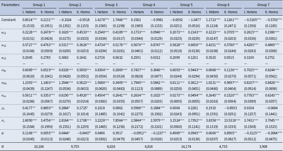
Note: ***, **, and * denote 1%, 5%, and 10% level of significance, respectively. Numbers in parentheses are the bootstrapped standard errors based on 200 replications.

A comparison of the input–output elasticities across groups reveals notable differences between the heterogeneous and homogeneous input price models. Specifically, Groups 2, 3, 4, and 6 exhibit more pronounced discrepancies in the estimated elasticities, suggesting that these groups are particularly sensitive to the assumption of input price heterogeneity.

Our discussion will primarily focus on the estimation results derived from the heterogeneous input price model, as it better reflects the underlying variations in input costs across industries and provides a more nuanced understanding of input–output relationships.

This table presents a detailed overview of the key parameters and outcomes derived from our model for all the groups under consideration. Each column of the table corresponds to a specific group, while each row highlights the estimated values for various parameters such as the elasticity of substitution, MRP of inputs, and the degree of misallocation for capital, labor, and materials. Thus, Table 3 provides a straightforward and brief overview of the impact and contribution of various industry groups to input misallocation. This comprehensive analysis is crucial for pinpointing sectors that could gain the most from better resource distribution and for directing future policy measures to boost productivity.

Our estimates of the parameter $\sigma _{s}$ in the CES aggregate production function, as specified in equation (3), range from 2.61 to 3.74 for Groups 1 to 7. This parameter, $\sigma _{s}$ , represents the elasticity of substitution between differentiated outputs within an industry.

In previous studies, this parameter has often been set to specific values based on either empirical findings or theoretical assumptions. For example, Hsieh and Klenow (2009) set $\sigma _{s}$ at 3 in their paper on misallocation and manufacturing TFP in China and India. Similarly, Gopinath et al. (2017) used the same value of 3 in their analysis of capital distribution and productivity in Southern Europe. More recently, Bils et al. (2021) set $\sigma _{s}$ at a slightly higher value of 4 in their study of factor shares and productivity.

According to Hsieh and Klenow (2009), the estimated TFP gains from reallocation are highly sensitive to this elasticity $\sigma _{s}$ . They found that China’s hypothetical TFP gain in 2005 increases from 87% under $\sigma _{s} =3$ to 184% with $\sigma _{s}=5$ , and India’s in 1994 increased from 128% to 230%. When $\sigma _{s}$ is higher, the convergence of TFPR gaps slows in response to the reallocation of inputs from low to high TFPR plants, resulting in greater potential gains from equalizing TFPR levels.

The variation in our estimated values of $\sigma _{s}$ , which range between 2.61 and 3.74, suggests that the elasticity of substitution may differ across different groups or sectors, reflecting varying degrees of flexibility in response to input reallocation. These estimates are slightly lower than the values commonly assumed in the literature, indicating that, for some groups, the ability to substitute between differentiated outputs may be more constrained than previously thought. This has important implications for understanding the dynamics of input misallocation and the potential productivity gains from more efficient resource allocation within these groups.

Table 3 provides crucial insights into the variability and significance of the misallocation terms and dynamic adjustment parameters across different groups within the manufacturing sector. Specifically, the table reports the variances of $\zeta _{Ksi}$ and $\zeta _{Msi}$ (denoted as $\sigma _{Ks}$ and $\sigma _{Ms}$ , respectively). The results indicate that these misallocation variances vary significantly across the groups analyzed. The statistical significance of $\sigma _{Ks}$ and $\sigma _{Ms}$ shows the importance of accounting for firm-specific misallocation when assessing overall productivity. The differences in these parameters across groups suggest that some sectors may experience more pronounced misallocation issues, which in turn can have a substantial impact on those sectors’ productivity and, by extension, on aggregate economic performance. This variation also highlights the need for targeted policy interventions that address the unique misallocation challenges faced by different industries.

In addition to the misallocation terms, Table 3 also reports the dynamic adjustment parameter in TFPR, denoted as $\rho _s$ . This parameter reflects the persistence or inertia in the revenue-based total factor productivity (TFPR) over time within a group. The values of $\rho _s$ vary substantially across the groups, and these variations are statistically significant. This finding indicates that the dynamic behavior of TFPR is not uniform across sectors—some groups exhibit higher levels of persistence, meaning that past productivity levels have a more prolonged influence on current productivity. In contrast, other groups may show more rapid adjustments in TFPR, suggesting that productivity in these sectors is more responsive to changes in input allocation or external shocks.

The substantial variation in $\rho _s$ across groups also points to the existence of different underlying mechanisms driving productivity dynamics in different sectors. For instance, industries with high $\rho _s$ values might be characterized by longer production cycles or more rigid structures, making it harder for them to adapt quickly to changes. In contrast, industries with lower values of $\rho _s$ might be more flexible and better able to adjust their production processes in response to changing conditions. The estimate of $\phi$ can be used to test the endogeneity of $\ln R$ . With the exception of Group 3, all $\hat {\phi }$ values are highly significant across the other groups, indicating the presence of endogeneity in the revenue variable.

The upper left panel of Figure 1 provides a dynamic visual representation of the distribution of revenue output among the seven groups analyzed during the sample period. This panel captures the relative contribution of each group to overall revenue, providing insight into how output is distributed among different segments of the manufacturing sector. By examining this panel, one can observe the variations in revenue shares across groups, noticing which sectors are more dominant in terms of output and how this distribution might have evolved over time.

Figure 1. Shares of $PY$ , $K$ , $L$ , and $M$ of groups 1–7 from 1975 to 2010

The remaining three panels in Figure 1 complement this analysis by illustrating the allocation of capital ( $K$ ), labor ( $L$ ), and materials ( $M$ ) in the same seven groups. Each of these panels presents the proportion of each input that is used by the different groups, providing a detailed view of how resources are distributed within the manufacturing sector. These panels are crucial for understanding the relationship between input allocation and revenue generation, as they allow for a comparison of whether groups with higher revenue shares are also those that receive a larger portion of the inputs.

By analyzing input allocation alongside revenue shares, these panels help identify potential misallocations of resources. For example, if a group with a relatively low share of revenue is receiving a disproportionately high share of one or more inputs, it could indicate inefficiencies in resource distribution. Conversely, if a group with a high revenue share is allocated fewer inputs, it might suggest that the group is operating more efficiently or is more productive with the resources it has.

The subgraphs in the upper panel of Figure 2 illustrate the comparison between the actual capital allocation weight and the optimal capital allocation weight across Groups 1 to 7. These weights are derived using the formulas provided in equations (25) and (26), which calculate the proportion of total capital allocated to each group relative to the theoretically optimal distribution based on the predictions of our model. By visualizing these weights, the graphs allow us to assess the extent of misallocation within each group, highlighting discrepancies between the current capital distribution and what would be considered efficient under optimal conditions.

Figure 2. Allocation weights of $K$ and $M$ for groups 1–7 from 1975 to 2010

Similarly, the subgraphs in the lower panel of Figure 2 present comparisons of the material allocation weight against the optimal material allocation weight for Groups 1 to 7. These weights, also calculated using equations (25) and (26), represent the share of total materials allocated to each group versus the optimal distribution as suggested by our model. The visual comparison in these graphs enables us to identify patterns of material misallocation, revealing how closely the actual allocation of materials aligns with the optimal scenario.

The upper panel of Figure 3 illustrates the temporal dynamics of $\overline {MRPK}_{K,s}$ and $\overline {MRPK}^*_{K,s}$ , where their ratio, $\gamma _{K}$ , compares the actual and optimal marginal revenue products of capital (MRPK) across sectors. This comparison provides insights into key misallocation patterns in capital allocation. The lower panel of Figure 3 highlights material allocation patterns, with deviations from unity indicating inefficiencies in capital or material usage. Collectively, these panels emphasize the sector-specific nature of misallocation, demonstrating that inefficiencies vary significantly across industries. By addressing these misallocations, particularly in sectors with pronounced discrepancies in capital and material inputs, targeted policy interventions could significantly enhance aggregate productivity. These findings underscore the potential gains from reducing misallocation to improve overall economic efficiency and sectoral performance.

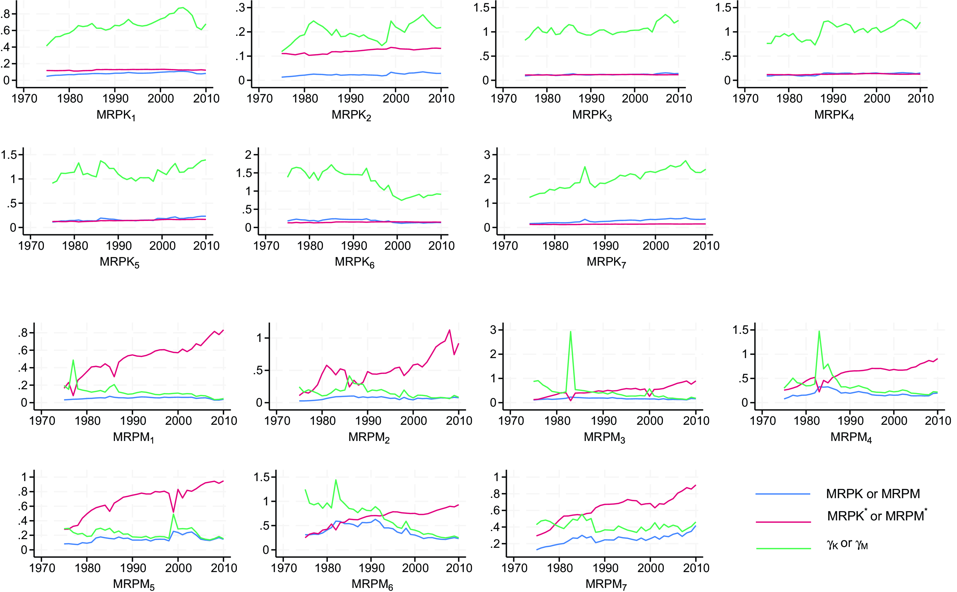
Figure 3. MRPK, MRPM and the ratios of MRPK and MRPM for groups 1–7 from 1975 to 2010

Figure 4 presents a detailed examination of the efficiency of allocation in the seven groups of the manufacturing sector, as evaluated using the equation specified in (30). An allocation is fully efficient when $AE=1$ . This figure is central to understanding how well resources are being utilized within each group relative to the optimal allocation that would maximize productivity. We used the estimation results from the homogeneous input price model in Table 3 to calculate allocative efficiency. Overall, the time trends of allocative efficiency estimated under both the homogeneous and heterogeneous input price assumptions appear largely consistent. However, the allocative efficiencies across all groups under the homogeneous input price assumption are significantly higher. This finding aligns with the results of Bils et al. (2021), where the assumption of homogeneous input prices was maintained. These observations suggest that the homogeneous input price assumption may lead to overestimation of allocative efficiency. A similar result was also found in De Loecker (2011), where he found that correcting for unobserved prices leads to substantially lower productivity gains. By comparison, the heterogeneous input price model provides a more detailed perspective, capturing variations in input prices across sectors and reflecting a more realistic measure of allocative efficiency.

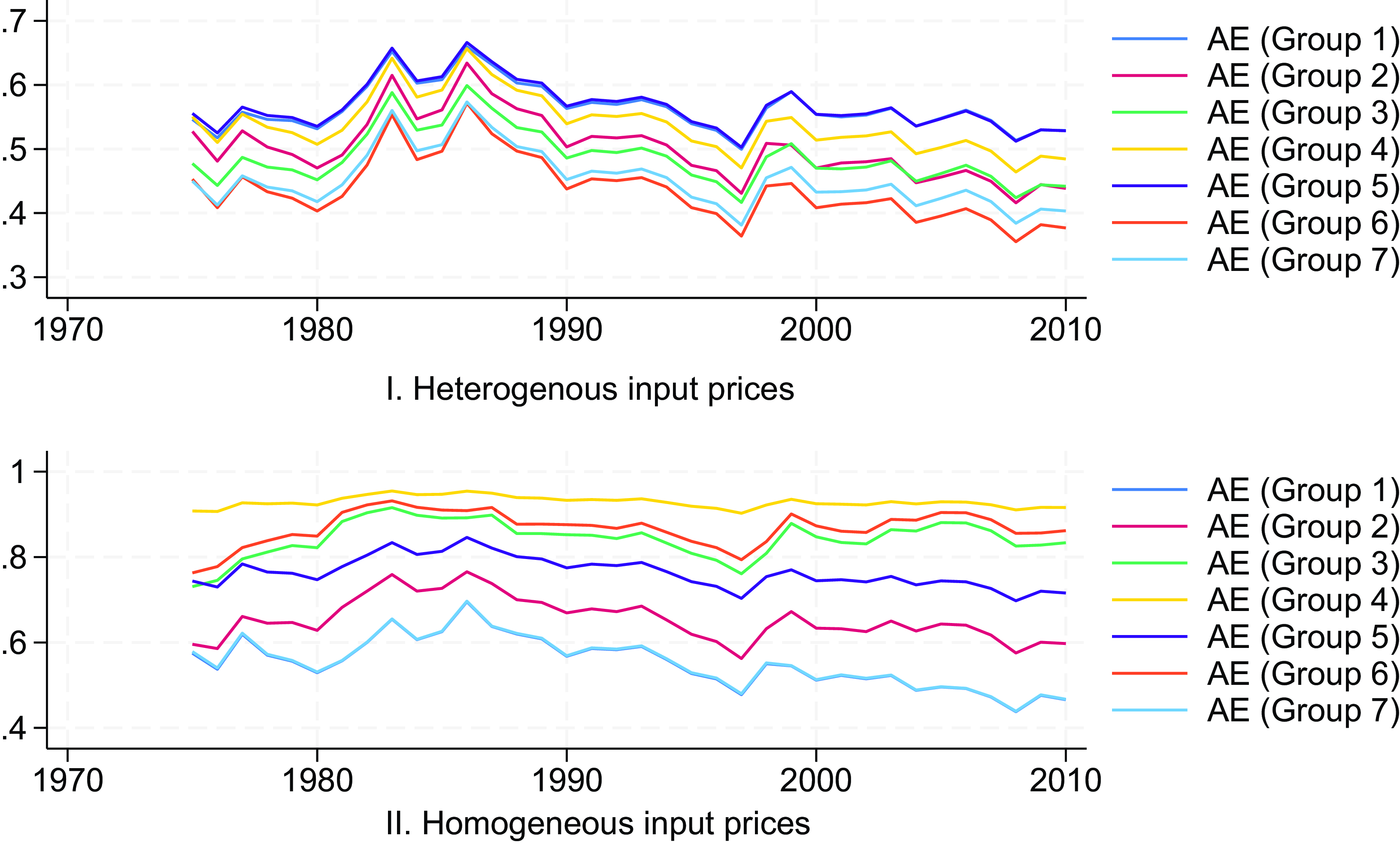
Figure 4. Allocation efficiency for groups 1–7 from 1975 to 2010

In the context of this analysis, AE measures the degree to which the actual distribution of inputs—capital ( $K$ ), labor ( $L$ ), and materials ( $M$ )—within each group aligns with the ideal distribution that would lead to the highest possible output or productivity. A higher value of $AE$ indicates that a group is effectively using its inputs in a manner close to the optimal scenario, minimizing waste, and maximizing output. In contrast, lower efficiency values suggest that there are significant deviations from the optimal input allocation, leading to potential productivity losses.

The results shown in Figure 4 reveal variations in $AE$ between the groups. For some groups, the AE may be relatively high, indicating that they are utilizing their input close to the optimal level. On the other hand, groups with lower AEs are identified as having suboptimal input distributions, which could be due to various factors such as market imperfections, regulatory constraints, or lack of access to necessary resources. These inefficiencies suggest that there is room for significant improvement in how resources are allocated, and addressing these issues could lead to substantial gains in productivity. This figure highlights the importance of efficient resource allocation in driving productivity and highlights the potential gains that could be realized by optimizing input use across the different segments of the manufacturing industry.

The observed trends of rising and falling aggregate efficiency in Figure 4 align with macroeconomic literature. First, economic recoveries often lead to reallocations of resources toward more productive firms, a “cleansing effect” described by Caballero and Hammour (1994). The efficiency gains observed in the early 1980s likely reflect post-recession adjustments after the stagflation period. Second, the late 1990s efficiency surge corresponds to the tech boom, where advancements in information technology reduced costs and improved resource allocation, as noted by Oliner and Sichel (2000). Third, the declines in efficiency observed during the early 2000s and the 2007–2009 financial crisis were likely driven by disruptions such as the Dot-Com Bust and tight credit markets, which led to significant resource misallocation and operational inefficiencies. These periods of economic turbulence were characterized by market uncertainty and constrained access to capital, further exacerbating inefficiencies in production and investment decisions.

We further compute the loss of revenue output due to misallocation, which is defined as the percentage loss of the group-specific efficient output, that is, $(1-AE_{s})*100\%$ . We summarize the results for the models under both heterogeneous and homogeneous input price assumptions at 5-year intervals, spanning from 1975 to 2010, in Table 4. The results also indicate that under the homogeneous input price assumption, the losses caused by the suboptimal allocation of production inputs are relatively overestimated.

Table 4. Loss of revenue output due to misallocation

Note: Loss of revenue output is defined as (1-AE)*100%.

Figure 5 illustrates the dynamic behavior of the logarithm of revenue-based total factor productivity (TFPR) for each group, represented as $\ln (TFPR_{s})$ , alongside the logarithm of efficient TFPR, denoted as $\ln (TFPR_{s}^{*})$ , for $s = 1, \dots, 7$ .

Figure 5. Ln(TFPR) and efficient ln(TFPR) of groups 1–7 from 1975 to 2010

This dynamic comparison allows us to visualize how the actual TFPR for each group diverges from the theoretically optimal TFPR, providing insights into the efficiency of resource allocation within each group over the study period. The graph highlights periods where significant misallocation may have occurred, as indicated by a widening gap between the actual and efficient TFPR lines, and, conversely, periods of more efficient allocation when these lines converge.

In Figure 6, we further explore the implications of this misallocation by comparing the aggregate revenue output across the seven groups. The blue line in this figure represents the actual aggregate revenue output, calculated by summing the revenue output of each group based on the existing input allocation. In contrast, the red line depicts the aggregate revenue output that would have been achieved if inputs had been allocated optimally across all groups, as derived from our model’s predictions. The difference between these two lines over time provides a visual representation of the potential productivity gains that could be realized through more efficient resource allocation.

Figure 6. Aggregate revenue output and allocation efficiency from 1975 to 2010

Additionally, Figure 7 includes a measure of aggregate AE, which is calculated using equation (32). This efficiency metric quantifies the degree to which actual resource allocation falls short of the optimal scenario, offering a single value that summarizes the overall efficiency of resource distribution across the entire economy. The AE measure is crucial for understanding the broader economic impact of input misallocation, as it directly relates to the potential increase in aggregate revenue output that could be achieved by reallocating inputs more effectively.

Figure 7. Aggregate ln(TFPR) and efficient ln(TFPR) from 1975 to 2010

Together, Figures 4 and 7 offer a comprehensive view of both group-specific and aggregate-level misallocation dynamics. By visualizing the actual versus optimal TFPR and revenue outputs, these figures help to clarify where inefficiencies lie, how they evolve over time, and the scale of the economic benefits that could be gained from improving resource allocation across the economy.

Figure 7 provides a comparative analysis of the aggregate logarithm of revenue-based TFP, $\ln (TFPR)$ , and the logarithm of the efficient aggregate TFPR, $\ln (TFPR^{*})$ , over the period from 1975 to 2010. This figure is crucial in illustrating the broader trends in productivity growth across the economy when considering actual versus optimal resource allocation.

The graph presents two distinct lines. One line represents the actual aggregate $\ln (TFPR)$ , which is the cumulative measure of productivity derived from the observed allocation of inputs between all firms within the study. The other line represents $\ln (TFPR^{*})$ , which is the hypothetical productivity level that could have been achieved if the inputs had been perfectly allocated according to the predictions of the model.

To quantify the difference in productivity growth between the actual and optimal scenarios, we calculate the average growth rate of $\ln (TFPR)$ and $\ln (TFPR^{*})$ during the study period. This average growth rate is determined by regressing the logarithm of the TFPR on time and thus capturing the trend of productivity growth. Our analysis reveals that the average growth rate of the actual aggregate TFPR from 1975 to 2010 is approximately 2.8%. In contrast, if inputs had been optimally allocated according to the efficient scenario, the average growth rate of the aggregate TFPR could have been as high as 3.2%.

This comparison highlights the significant impact of input misallocation on overall productivity growth. The gap between actual and optimal growth rates, as illustrated by the two lines in Figure 7, underscores the potential productivity gains that remain unrealized due to inefficiencies in resource allocation. During the 35-year period, these seemingly small differences in annual growth rates accumulate, leading to substantial differences in aggregate productivity levels.

Thus, Figure 7 not only provides a visual representation of the historical trends in aggregate productivity, but also emphasizes the economic importance of improving resource allocation. By addressing the inefficiencies that contribute to the divergence between $\ln (TFPR)$ and $\ln (TFPR^{*})$ , policymakers and firms could potentially unlock significant productivity gains, driving more robust economic growth over time.

6. Conclusion

In this paper, we propose a model for estimating input misallocation based on the firm’s profit maximization problem. The model is designed to capture the intricacies of how firms allocate resources, acknowledging that these decisions are influenced by various factors such as varying input prices and the specific composition of inputs used in production. Building on the HK model, our approach introduces several key enhancements that allow for a more accurate and comprehensive analysis of resource AE.

First, our model extends the HK framework by incorporating heterogeneity in input prices across firms. This extension acknowledges that firms do not operate under uniform conditions: factors such as market power, location, and access to resources result in different input prices for different firms. In addition, we refine the input structure by including three distinct inputs: capital, labor, and materials. This more detailed input structure enables us to better capture the complexities of production processes at the firm level and the resulting inefficiencies that may arise from misallocation.

Second, rather than relying on calibration, we employ a rigorous econometric approach to estimate the model parameters. The estimation of model parameters and AE is based on the system of input demand and the production function. The restricted coefficients in the demand system complicate the MLE, especially with numerous constraints. To overcome these challenges, we use an indirect inference procedure. This method allows us to estimate the derived input demand function from the firm’s optimization problem, making the analysis endogenous and directly tied to the economic behavior of firms. By estimating these parameters using firm-level data, we are able to provide a clearer and better understanding of how misallocation impacts productivity. The resulting estimates of firm-specific misallocation, MRPs of inputs, and measures of total factor productivity (TFPR and TFPQ) are then aggregated to provide insight at the sectoral and industry levels.

Our findings highlight significant productivity losses due to resource misallocation. Specifically, we observe that the average productivity growth rate (TFPR) from 1975 to 2010 was approximately 2.7%. However, our counterfactual analysis indicates that this growth rate could have reached 3.5% with optimal input allocation. This disparity underscores the substantial economic cost of misallocation and suggests that policies aimed at reducing these inefficiencies could lead to notable improvements in overall economic performance.

Our focus, distinct from the models mentioned above, is primarily on the input allocation at the firm level. We analyze the revenue loss resulting from misallocation at the firm level, which is then used to assess the revenue loss at the aggregate level.

By offering a more granular analysis of firm-level misallocation and its aggregate effects, our study makes a valuable contribution to the ongoing discourse on the determinants of productivity and the role of resource allocation in driving economic growth. It not only provides empirical evidence of the magnitude of misallocation’s impact on productivity, but also offers a framework for assessing and potentially improving AE across firms. Our findings have important implications for policymakers, as they suggest that targeted interventions to enhance resource allocation could yield substantial benefits for the economy as a whole.