


1. Introduction
Throughout this paper, $G=(V,E)$
denotes an undirected connected plane graph, which may have multiple edges, but no self-loops. Given a vertex
$G=(V,E)$
denotes an undirected connected plane graph, which may have multiple edges, but no self-loops. Given a vertex $v\in V$
and an edge
$v\in V$
and an edge $e=(u,v) \in E$
, the left-edge of e (at v) is the edge
$e=(u,v) \in E$
, the left-edge of e (at v) is the edge $e_1=(u_1,v)$
that follows e (at v) in clockwise (cw) direction, the right-edge of e (at v) is the edge
$e_1=(u_1,v)$
that follows e (at v) in clockwise (cw) direction, the right-edge of e (at v) is the edge $e_2=(u_2,v)$
that follows e (at v) in counter-clockwise (ccw) direction.
$e_2=(u_2,v)$
that follows e (at v) in counter-clockwise (ccw) direction.
A walk of G is a sequence $P=v_0 e_1 v_1 e_2 \ldots e_k v_k$
where
$P=v_0 e_1 v_1 e_2 \ldots e_k v_k$
where $v_i$
are vertices of G (may be repeated) and
$v_i$
are vertices of G (may be repeated) and $e_j =(v_{j-1},v_j)$
are distinct edges of G. The length of P is k. If
$e_j =(v_{j-1},v_j)$
are distinct edges of G. The length of P is k. If $v_0=v_k$
, P is called a tour. A walk (tour, respectively) consisting of distinct vertices is called a path (cycle, respectively). A walk is called a Petrie walk if the edge
$v_0=v_k$
, P is called a tour. A walk (tour, respectively) consisting of distinct vertices is called a path (cycle, respectively). A walk is called a Petrie walk if the edge $e_{i+1}$
is alternately the left- and the right-edge of
$e_{i+1}$
is alternately the left- and the right-edge of $e_i$
for
$e_i$
for $1\leq i <k$
. A tour P is called a Petrie tour if it is a Petrie walk, and the alternating left- and right-edge condition also holds for
$1\leq i <k$
. A tour P is called a Petrie tour if it is a Petrie walk, and the alternating left- and right-edge condition also holds for $e_{k-1}$
,
$e_{k-1}$
, $e_k,$
and
$e_k,$
and $e_1$
. Petrie path and Petrie cycle are defined similarly. Petrie walks are also called left-right paths and studied in Shank (Reference Shank1975).
$e_1$
. Petrie path and Petrie cycle are defined similarly. Petrie walks are also called left-right paths and studied in Shank (Reference Shank1975).
A Petrie cycle partition of G is a set ${\mathscr C}=\{ C_1, \ldots, C_p\}$
of Petrie cycles such that each vertex of G is in exactly one
${\mathscr C}=\{ C_1, \ldots, C_p\}$
of Petrie cycles such that each vertex of G is in exactly one $C_i\in {\mathscr C}$
. If
$C_i\in {\mathscr C}$
. If ${\mathscr C}$
consists of a single cycle
${\mathscr C}$
consists of a single cycle $C_1$
,
$C_1$
, $C_1$
is call a Petrie Hamiltonian cycle of G. The properties of graphs with Petrie Hamiltonian cycle have been studied in Fouquet et al. (1982), IvanÇo and Jendrol’ (1999), Ivančo et al. (Reference Ivančo, Jendrol’ and Tkśč1994).
$C_1$
is call a Petrie Hamiltonian cycle of G. The properties of graphs with Petrie Hamiltonian cycle have been studied in Fouquet et al. (1982), IvanÇo and Jendrol’ (1999), Ivančo et al. (Reference Ivančo, Jendrol’ and Tkśč1994).
A Petrie tour partition of G is a set ${\mathscr P}=\{ P_1, \ldots, P_q\}$
of Petrie tours such that each edge of G is in exactly one
${\mathscr P}=\{ P_1, \ldots, P_q\}$
of Petrie tours such that each edge of G is in exactly one $P_i\in {\mathscr P}$
. If
$P_i\in {\mathscr P}$
. If ${\mathscr P}$
consists of a single tour
${\mathscr P}$
consists of a single tour $P_1$
,
$P_1$
, $P_1$
is call a Petrie Eulerian tour of G. The properties of graphs with Petrie Eulerian tours have been studied in Kidwell and Bruce Richter (Reference Kidwell and Bruce Richter1987), Žitnik (Reference Žitnik2002).
$P_1$
is call a Petrie Eulerian tour of G. The properties of graphs with Petrie Eulerian tours have been studied in Kidwell and Bruce Richter (Reference Kidwell and Bruce Richter1987), Žitnik (Reference Žitnik2002).
In this paper, we study the properties of 3-regular plane graphs that have Petrie cycle partitions and the properties of 4-regular plane graphs that have Petrie tour partitions. For reasons that will become clear later, the 3-regular plane graph contains no multiple edges, but 4-regular plane graphs may contain multiple edges. We describe a simple characterization for 3-regular plane graphs with Petrie cycle partitions. This extends the results on plane graphs with Petrie Hamiltonian cycles in Fouquet et al. (1982), IvanÇo and Jendrol’ (1999), Ivančo et al. (Reference Ivančo, Jendrol’ and Tkśč1994). We describe a simple characterization for 4-regular plane graphs with Petrie tour partitions. This extends the results on plane graphs with Petrie Eulerian tours in Kidwell and Bruce Richter (Reference Kidwell and Bruce Richter1987), Žitnik (Reference Žitnik2002).
We also study the properties of Petrie partitionable graphs (as defined in the abstract). The general version of this problem is motivated by a data compression method, tristrip, used in computer graphics. We present a nice characterization of such graphs and show that the problem of determining if G is Petrie partitionable is NP-complete.
The present paper is organized as follows. Section 2 introduces the definitions and the motivation of these problems in computer graphics. Section 3 discusses the Petrie cycle partition of 3-regular plane graphs. Section 4 considers the Petrie tour partition of 4-regular plane graphs. The results in Sections 3 and 4 are relatively easy generalizations of known results in Fouquet et al. (1982), IvanÇo and Jendrol’ (1999), Ivančo et al. (Reference Ivančo, Jendrol’ and Tkśč1994), Kidwell and Bruce Richter (Reference Kidwell and Bruce Richter1987), Žitnik (Reference Žitnik2002). To the best of our knowledge, they have not been published in literature. Since they are of independent interests and also needed by the discussion in Section 5, we include these results here. Section 5 describes a nice characterization of Petrie partitionable 4-regular plane graphs. In Section 6, we show the problem of determining if a input 4-regular plane graph is Petrie partitionable is NP-complete. Section 7 describes some open problems and concludes the paper.
2. Definitions and Motivations
In this section, we give definitions and preliminary results. We use standard terminology in Bondy and Murty (Reference Bondy and Murty1979). Let $G=(V,E)$
be an undirected graph with n vertices and m edges. The degree of a vertex
$G=(V,E)$
be an undirected graph with n vertices and m edges. The degree of a vertex $v\in V$
, denoted by
$v\in V$
, denoted by $\deg(v)$
, is the number of edges incident to v. G is called 3-regular (4-regular, respectively), if
$\deg(v)$
, is the number of edges incident to v. G is called 3-regular (4-regular, respectively), if $\deg(v)=3$
(
$\deg(v)=3$
( $\deg(v)=4$
, respectively) for all
$\deg(v)=4$
, respectively) for all $v\in V$
. For a subset
$v\in V$
. For a subset $E_1 \subseteq E$
, the subgraph of G induced by
$E_1 \subseteq E$
, the subgraph of G induced by $E_1$
consists of
$E_1$
consists of $E_1$
as its edge set and the set of the vertices incident to the edges in
$E_1$
as its edge set and the set of the vertices incident to the edges in $E_1$
as its vertex set. G is bipartite if V can be partitioned into two subsets
$E_1$
as its vertex set. G is bipartite if V can be partitioned into two subsets $V_1$
and
$V_1$
and $V_2$
such that no two vertices in
$V_2$
such that no two vertices in $V_1$
are adjacent and no two vertices in
$V_1$
are adjacent and no two vertices in $V_2$
are adjacent. A k-vertex-coloring of G is a coloring of V by k colors so that any two adjacent vertices have different colors. A k-edge-coloring of G is a coloring of E by k colors so that any two edges incident to the same vertex have different colors.
$V_2$
are adjacent. A k-vertex-coloring of G is a coloring of V by k colors so that any two adjacent vertices have different colors. A k-edge-coloring of G is a coloring of E by k colors so that any two edges incident to the same vertex have different colors.
A plane graph G is a graph embedded in the plane without edge crossings (i.e. an embedded planar graph). The embedding of a plane graph G divides the plane into a number of regions called faces. The unbounded region is the exterior face. Other regions are interior faces. ${\mathscr F}$
denotes the set of the faces of G. For each face
${\mathscr F}$
denotes the set of the faces of G. For each face $F\in {\mathscr F}$
,
$F\in {\mathscr F}$
, $\deg(F)$
is the number of edges on the boundary of F. It is well known that a plane graph G is bipartite if and only if
$\deg(F)$
is the number of edges on the boundary of F. It is well known that a plane graph G is bipartite if and only if $\deg(F)$
is even for all
$\deg(F)$
is even for all $F\in {\mathscr F}$
(Bondy and Murty Reference Bondy and Murty1979). A k-face-coloring of a plane graph G is a coloring of its faces by k colors so that any two faces sharing an edge as their common boundary have different colors.
$F\in {\mathscr F}$
(Bondy and Murty Reference Bondy and Murty1979). A k-face-coloring of a plane graph G is a coloring of its faces by k colors so that any two faces sharing an edge as their common boundary have different colors.
A plane graph G is called a triangulation (quadrangulation, respectively), if $\deg(F) =3$
(
$\deg(F) =3$
( $\deg(F) =4$
, respectively) for all faces
$\deg(F) =4$
, respectively) for all faces $F\in {\mathscr F}$
.
$F\in {\mathscr F}$
.
The dual graph $G^*=(V^*,E^*)$
of a plane graph
$G^*=(V^*,E^*)$
of a plane graph $G=(V,E)$
is defined as follows: For each face F of G,
$G=(V,E)$
is defined as follows: For each face F of G, $V^*$
has a vertex
$V^*$
has a vertex $v_F$
. For each edge e in G,
$v_F$
. For each edge e in G, $G^*$
has an edge
$G^*$
has an edge $e^*=(v_{F_1},v_{F_2})$
where
$e^*=(v_{F_1},v_{F_2})$
where $F_1$
and
$F_1$
and $F_2$
are the two faces of G with e on their common boundary.
$F_2$
are the two faces of G with e on their common boundary. $e^*$
is called the dual edge of e. The mapping
$e^*$
is called the dual edge of e. The mapping $e \leftrightarrow e^*$
is a one-to-one correspondence between E and
$e \leftrightarrow e^*$
is a one-to-one correspondence between E and $E^*$
. G is a triangulation (quadrangulation, respectively) if and only if
$E^*$
. G is a triangulation (quadrangulation, respectively) if and only if $G^*$
is 3-regular (4-regular, respectively).
$G^*$
is 3-regular (4-regular, respectively).
2.1 Motivation
The problem studied in this paper is motivated by a data compression technique used in computer graphics. 3D objects are often represented by triangular mashes in computer graphics. For our purpose, this is just a plane triangulation $\tilde{G}=(\tilde{V},\tilde{E})$
. Following the terms used in computer graphics, the members of the vertex set
$\tilde{G}=(\tilde{V},\tilde{E})$
. Following the terms used in computer graphics, the members of the vertex set $\tilde{V}=\{ 1,2,\ldots,n\}$
are called points. An important problem in computer graphics is how to represent
$\tilde{V}=\{ 1,2,\ldots,n\}$
are called points. An important problem in computer graphics is how to represent $\tilde{G}$
efficiently. As a straightforward method, each face of
$\tilde{G}$
efficiently. As a straightforward method, each face of $\tilde{G}$
can be represented by listing its three boundary points. If
$\tilde{G}$
can be represented by listing its three boundary points. If $\tilde{G}$
has N faces, this representation uses 3N points. For large 3D objects, this takes too much space. The tristrips representation of
$\tilde{G}$
has N faces, this representation uses 3N points. For large 3D objects, this takes too much space. The tristrips representation of $\tilde{G}$
was discussed in Xiang et al. (Reference Xiang, Held and Mitchell1999). A tristrip is a sequence
$\tilde{G}$
was discussed in Xiang et al. (Reference Xiang, Held and Mitchell1999). A tristrip is a sequence ${\mathscr T}=F_1 F_2 \ldots F_t$
of faces in
${\mathscr T}=F_1 F_2 \ldots F_t$
of faces in $\tilde{G}$
, which can be represented by a sequence
$\tilde{G}$
, which can be represented by a sequence $S_{{\mathscr T}}=v_1v_2\ldots v_{t+2}$
of points of
$S_{{\mathscr T}}=v_1v_2\ldots v_{t+2}$
of points of $\tilde{G}$
in such a way that, for each i (
$\tilde{G}$
in such a way that, for each i ( $1\leq i \leq t$
), the three points
$1\leq i \leq t$
), the three points $v_iv_{i+1}v_{i+2}$
are the boundary points of the face
$v_iv_{i+1}v_{i+2}$
are the boundary points of the face $F_i$
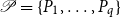
. An example of tristrip is shown in Figure 1A. A tristrip
$F_i$
. An example of tristrip is shown in Figure 1A. A tristrip ${\mathscr T}=F_1 \ldots F_t$
is called a tristrip cycle, represented by the point sequence
${\mathscr T}=F_1 \ldots F_t$
is called a tristrip cycle, represented by the point sequence $S_{{\mathscr T}}=v_1v_2\ldots v_t$
, if both
$S_{{\mathscr T}}=v_1v_2\ldots v_t$
, if both ${\mathscr T}$
and
${\mathscr T}$
and $S_{{\mathscr T}}$
are regarded as cyclic sequences and every three consecutive points
$S_{{\mathscr T}}$
are regarded as cyclic sequences and every three consecutive points $v_iv_{i+1}v_{i+2}$
(
$v_iv_{i+1}v_{i+2}$
( $1\leq i \leq t$
) are the boundary points of the face
$1\leq i \leq t$
) are the boundary points of the face $F_i$
. (Here we define
$F_i$
. (Here we define $t+1 =1$
and
$t+1 =1$
and $t+2=2$
). An example of tristrip cycle is shown in Figure 1B. Thus, by using a tristrip, t faces in
$t+2=2$
). An example of tristrip cycle is shown in Figure 1B. Thus, by using a tristrip, t faces in ${\mathscr T}$
are represented by
${\mathscr T}$
are represented by $S_{{\mathscr T}}$
of
$S_{{\mathscr T}}$
of $t+2$
points (t points for a tristrip cycle).
$t+2$
points (t points for a tristrip cycle).

Figure 1. (A) A tristrip ${\mathscr T}=F_1F_2F_3F_4F_5F_6F_7$
represented by
${\mathscr T}=F_1F_2F_3F_4F_5F_6F_7$
represented by ${\mathscr S}_{{\mathscr T}}=123456371$
. (B) A tristrip cycle
${\mathscr S}_{{\mathscr T}}=123456371$
. (B) A tristrip cycle ${\mathscr T}=F_1F_2F_3F_4F_5F_6$
represented by
${\mathscr T}=F_1F_2F_3F_4F_5F_6$
represented by ${\mathscr S}_{{\mathscr T}}=123456$
. (The solid thin lines are the edges of the triangular mesh
${\mathscr S}_{{\mathscr T}}=123456$
. (The solid thin lines are the edges of the triangular mesh $\tilde{G}$
. The small black squares are the vertices of the dual graph G. The thick dashed lines are the edges of
$\tilde{G}$
. The small black squares are the vertices of the dual graph G. The thick dashed lines are the edges of ${\mathscr T}$
. The thick doted lines are the edges of G, not in
${\mathscr T}$
. The thick doted lines are the edges of G, not in ${\mathscr T}$
).
${\mathscr T}$
).
If all faces of $\tilde{G}$
belong to one tristrip (or tristrip cycle), we can reduce the space for representing
$\tilde{G}$
belong to one tristrip (or tristrip cycle), we can reduce the space for representing $\tilde{G}$
by a factor of 3 (Estkowski et al. Reference Estkowski, Mitchell and Xiang2002). However, a typical triangular mesh
$\tilde{G}$
by a factor of 3 (Estkowski et al. Reference Estkowski, Mitchell and Xiang2002). However, a typical triangular mesh $\tilde{G}$
cannot be covered by one tristrip (or tristrip cycle). It is then a natural question: how to find the fewest disjoint tristrips (or tristrip cycles) that cover all faces of
$\tilde{G}$
cannot be covered by one tristrip (or tristrip cycle). It is then a natural question: how to find the fewest disjoint tristrips (or tristrip cycles) that cover all faces of $\tilde{G}$
? This minimization problem is known as Stripification problem in computer graphics. It was shown to be NP-complete in Estkowski et al. (Reference Estkowski, Mitchell and Xiang2002). Various heuristic and exact (exponential time) algorithms have been studied in Porcu and Scateni (Reference Porcu and Scateni2003), Šíma (Reference Šíma2005), Xiang et al. (Reference Xiang, Held and Mitchell1999).
$\tilde{G}$
? This minimization problem is known as Stripification problem in computer graphics. It was shown to be NP-complete in Estkowski et al. (Reference Estkowski, Mitchell and Xiang2002). Various heuristic and exact (exponential time) algorithms have been studied in Porcu and Scateni (Reference Porcu and Scateni2003), Šíma (Reference Šíma2005), Xiang et al. (Reference Xiang, Held and Mitchell1999).
The Stripification problem is closely related to the Petrie cycle partition problem as follows. Let $G=(V,E)$
be the dual graph of
$G=(V,E)$
be the dual graph of $\tilde{G}$
. Clearly, G is 3-regular. For each face F of
$\tilde{G}$
. Clearly, G is 3-regular. For each face F of $\tilde{G}$
, let
$\tilde{G}$
, let $v_F$
denote the vertex in G corresponding to F. Consider a sequence of faces
$v_F$
denote the vertex in G corresponding to F. Consider a sequence of faces ${\mathscr T}=F_1 \ldots F_t$
of
${\mathscr T}=F_1 \ldots F_t$
of $\tilde{G}$
. It is easy to see that
$\tilde{G}$
. It is easy to see that ${\mathscr T}$
is a tristrip (or tristrip cycle) of
${\mathscr T}$
is a tristrip (or tristrip cycle) of $\tilde{G}$
if and only if the corresponding sequence
$\tilde{G}$
if and only if the corresponding sequence $v_{F_1} \ldots v_{F_t}$
is a Petrie path (or Petrie cycle) in G. (See Figure 1A and B.) Hence, the problem of finding a minimum tristrip cycle partition for the faces of
$v_{F_1} \ldots v_{F_t}$
is a Petrie path (or Petrie cycle) in G. (See Figure 1A and B.) Hence, the problem of finding a minimum tristrip cycle partition for the faces of $\tilde{G}$
is the same as the problem of finding a minimum Petrie cycle partition for G.
$\tilde{G}$
is the same as the problem of finding a minimum Petrie cycle partition for G.
In computer graphics, 3D objects are also represented by quadrangular meshes (see Bommes et al. Reference Bommes, L’vy, Pietroni, Puppo, Silva, Tarini and Zorin2012, Reference Bommes, Campen, Ebke, Alliez and Kobbelt2013; Dong et al. 2006). For our purpose, this is just a plane quadrangulation $\tilde{G}=(\tilde{V},\tilde{E})$
. If we add a chord into each face of
$\tilde{G}=(\tilde{V},\tilde{E})$
. If we add a chord into each face of $\tilde{G}$
, it becomes a plane triangulation
$\tilde{G}$
, it becomes a plane triangulation $\tilde{G}_3$
which is called a triangular extension of
$\tilde{G}_3$
which is called a triangular extension of $\tilde{G}$
. Since each face F of
$\tilde{G}$
. Since each face F of $\tilde{G}$
has degree 4, there are two ways to add a chord into F. If
$\tilde{G}$
has degree 4, there are two ways to add a chord into F. If $\tilde{G}$
has
$\tilde{G}$
has $\tilde{f}$
faces, it has
$\tilde{f}$
faces, it has $2^{\tilde{f}}$
triangular extensions. One way to represent
$2^{\tilde{f}}$
triangular extensions. One way to represent $\tilde{G}$
is first convert it to a plane triangular extension
$\tilde{G}$
is first convert it to a plane triangular extension $\tilde{G}_3$
by adding chords into its faces and then represent
$\tilde{G}_3$
by adding chords into its faces and then represent $\tilde{G}_3$
by using tristrips or tristrip cycles (Estkowski et al. Reference Estkowski, Mitchell and Xiang2002). The question is: which of those
$\tilde{G}_3$
by using tristrips or tristrip cycles (Estkowski et al. Reference Estkowski, Mitchell and Xiang2002). The question is: which of those $2^{\tilde{f}}$
triangular extensions can be partitioned into a minimum number of tristrips (or tristrip cycles)?
$2^{\tilde{f}}$
triangular extensions can be partitioned into a minimum number of tristrips (or tristrip cycles)?
A special version of this problem is closely related to the Petrie tour partition problem. Consider the dual graph $G=(V,E)$
of
$G=(V,E)$
of $\tilde{G}$
. Clearly, G is 4-regular. Consider a vertex
$\tilde{G}$
. Clearly, G is 4-regular. Consider a vertex $v \in V$
corresponding to a face F in
$v \in V$
corresponding to a face F in $\tilde{G}$
. Let
$\tilde{G}$
. Let $e_1,e_2,e_3,e_4$
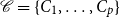
be the four edges incident to v in cw order. The split operation at v splits v into two degree-3 vertices v’ and v” as shown in Figure 2. There are two ways to split v. They correspond to the two ways of adding a chord into the face F. Let
$e_1,e_2,e_3,e_4$
be the four edges incident to v in cw order. The split operation at v splits v into two degree-3 vertices v’ and v” as shown in Figure 2. There are two ways to split v. They correspond to the two ways of adding a chord into the face F. Let $G_3$
be the 3-regular plane graph obtained by performing split operation at every vertex of G. We call
$G_3$
be the 3-regular plane graph obtained by performing split operation at every vertex of G. We call $G_3$
a 3-regularization of G. The edge (v’,v”) of
$G_3$
a 3-regularization of G. The edge (v’,v”) of $G_3$
introduced by splitting a vertex
$G_3$
introduced by splitting a vertex $v \in V$
is denoted by e(v) and called a split edge of
$v \in V$
is denoted by e(v) and called a split edge of $G_3$
.
$G_3$
.

Figure 2. (A) A vertex v in G corresponding to a face F in $\tilde{G}$
. (B) and (C) Two ways to split v.
$\tilde{G}$
. (B) and (C) Two ways to split v.
Suppose G has a Petrie tour partition ${\mathscr P}=\{P_1,\ldots,P_q\}$
. Consider any vertex
${\mathscr P}=\{P_1,\ldots,P_q\}$
. Consider any vertex $v\in V$
with four incident edges
$v\in V$
with four incident edges $e_1,e_2,e_3,e_4 \in E$
. Two tours
$e_1,e_2,e_3,e_4 \in E$
. Two tours $P_i$
and
$P_i$
and $P_j$
in
$P_j$
in ${\mathscr P}$
visit v (possibly
${\mathscr P}$
visit v (possibly $P_i=P_j$
). We split v so that
$P_i=P_j$
). We split v so that $P_i$
and
$P_i$
and $P_j$
are still tours after splitting. (See Figure 2B and C.) Do this at every vertex
$P_j$
are still tours after splitting. (See Figure 2B and C.) Do this at every vertex $v\in V$
. Let
$v\in V$
. Let $G_3$
be the resulting 3 regularization of G. It is easy to see that
$G_3$
be the resulting 3 regularization of G. It is easy to see that ${\mathscr P}=\{P_1,\ldots,P_q\}$
is a Petrie cycle partition of
${\mathscr P}=\{P_1,\ldots,P_q\}$
is a Petrie cycle partition of $G_3$
. Thus, if G has a Petrie tour partition, then G has a 3-regularization
$G_3$
. Thus, if G has a Petrie tour partition, then G has a 3-regularization $G_3$
with a Petrie cycle partition
$G_3$
with a Petrie cycle partition ${\mathscr P}$
, where every edge e of G belongs to a Petrie cycle in
${\mathscr P}$
, where every edge e of G belongs to a Petrie cycle in ${\mathscr P}$
. For its application in computer graphics, this restriction is not necessary. Figure 10A shows a 4-regular plane graph G which has no Petrie tour partition (as we will see later). However, it has a 3-regularization
${\mathscr P}$
. For its application in computer graphics, this restriction is not necessary. Figure 10A shows a 4-regular plane graph G which has no Petrie tour partition (as we will see later). However, it has a 3-regularization $G_3$
(shown in Figure 10B) which has a Petrie cycle partition with a single Petrie Hamiltonian cycle C. (Some edges of G are in C. Some are not). This motivates:
$G_3$
(shown in Figure 10B) which has a Petrie cycle partition with a single Petrie Hamiltonian cycle C. (Some edges of G are in C. Some are not). This motivates:
Definition 1. A 4-regular plane graphs G is called Petrie partitionable if it has a 3-regularization with a Petrie cycle partition.
A main interest of this paper is to characterize the Petrie partitionable graphs. In computer graphics applications, the problem is to find a 3-regularization G’ of G so that the faces of G’ can be partitioned into tristrips and/or tristrip cycles. The NP-hardness result in Estkowski et al. (Reference Estkowski, Mitchell and Xiang2002) suggests that this problem might be NP-hard also. The problem considered in this paper is a restricted version of the general problem: partition into Petrie cycles only. In contrast to the more general problem, this restriction leads to a simple characterization. The focus of our study is on the graph-theoretical properties of these problems. The insights obtained here may help to find more efficient algorithms for solving the general problem.
3. Characterization of 3-Regular Plane Graphs with Petrie Cycle Partition
In this section, $G=(V,E)$
always denotes a 3-regular connected plane simple graph (i.e. G has no self-loops nor parallel edges). Suppose G has a Petrie cycle partition
$G=(V,E)$
always denotes a 3-regular connected plane simple graph (i.e. G has no self-loops nor parallel edges). Suppose G has a Petrie cycle partition ${\mathscr C} = \{ C_1,\dots,C_p\}$
. For any vertex
${\mathscr C} = \{ C_1,\dots,C_p\}$
. For any vertex $v\in V$
, two edges incident to v belong to a cycle
$v\in V$
, two edges incident to v belong to a cycle $C_i \in {\mathscr C}$
and its third incident edge is not in any
$C_i \in {\mathscr C}$
and its third incident edge is not in any $C_j\in {\mathscr C}$
. We call the third edge a non-cycle edge with respect to
$C_j\in {\mathscr C}$
. We call the third edge a non-cycle edge with respect to ${\mathscr C}$
.
${\mathscr C}$
.
A 3-regular plane graph G is called a multi-3-gon if all of its faces have degrees divisible by 3. The following lemma was proved in IvanÇo and Jendrol’ (1999), Ivančo et al. (Reference Ivančo, Jendrol’ and Tkśč1994).
Lemma 1. If a 3-regular plane graph has a Petrie Hamiltonian cycle, then it is a multi-3-gon.
The following lemma generalizes Lemma 1. The proof is essentially the same as in IvanÇo and Jendrol’ (1999). We include it here for completeness.
Lemma 2. Any 3-regular plane graph G with a Petrie cycle partition must be a multi-3-gon.
Proof. Let ${\mathscr C} = \{ C_1,\ldots C_p\}$
be a Petrie cycle partition of G. Consider any face F of G and a cycle
${\mathscr C} = \{ C_1,\ldots C_p\}$
be a Petrie cycle partition of G. Consider any face F of G and a cycle $C_i\in {\mathscr C}$
that travels at least one edge of F. Suppose
$C_i\in {\mathscr C}$
that travels at least one edge of F. Suppose $C_i$
travels two edges
$C_i$
travels two edges $e_1=(u,v)$
and
$e_1=(u,v)$
and $e_2=(v,w)$
from u to v to w where
$e_2=(v,w)$
from u to v to w where $e_1$
is not an edge of F, but
$e_1$
is not an edge of F, but $e_2$
is an edge of F. Let
$e_2$
is an edge of F. Let $e_3=(w,x)$
and
$e_3=(w,x)$
and $e_4=(x,y)$
be the two edges of F following
$e_4=(x,y)$
be the two edges of F following $e_2$
in the direction from v to w. When
$e_2$
in the direction from v to w. When $C_i$
travels from
$C_i$
travels from $e_1$
to
$e_1$
to $e_2$
, suppose it turns left at v (see Figure 3A). Since
$e_2$
, suppose it turns left at v (see Figure 3A). Since $C_i$
is a Petrie cycle, it turns right at w and travels
$C_i$
is a Petrie cycle, it turns right at w and travels $e_3$
. Then,
$e_3$
. Then, $C_i$
must make a left-turn at x. So
$C_i$
must make a left-turn at x. So $e_4$
is a non-cycle edge with respect to
$e_4$
is a non-cycle edge with respect to ${\mathscr C}$
. If
${\mathscr C}$
. If $C_i$
turns right at v, it must turn left at w and travel
$C_i$
turns right at v, it must turn left at w and travel $e_3$
(Figure 3B). Then,
$e_3$
(Figure 3B). Then, $C_i$
must turn right at x. So
$C_i$
must turn right at x. So $e_4$
must be a non-cycle edge with respect to
$e_4$
must be a non-cycle edge with respect to ${\mathscr C}$
.
${\mathscr C}$
.

Figure 3. The proof of Lemma 2.
Thus, the edges on the boundary of F can be partitioned into subpaths of length 3: The first two edges of a subpath belong to a Petrie cycle $C_i\in {\mathscr C}$
, while the third edge of the subpath is a non-cycle edge. Hence, the length of F must be a multiple of 3.
$C_i\in {\mathscr C}$
, while the third edge of the subpath is a non-cycle edge. Hence, the length of F must be a multiple of 3. ![]()
If $G=(V,E)$
has a proper 3-edge-coloring
$G=(V,E)$
has a proper 3-edge-coloring $\lambda: E \rightarrow\{1,2,3\}$
, the Heawood valuation (or simply valuation) associated with
$\lambda: E \rightarrow\{1,2,3\}$
, the Heawood valuation (or simply valuation) associated with $\lambda$
is a mapping
$\lambda$
is a mapping $\lambda^*: V \rightarrow \{-1, 1 \}$
defined as follows. For any vertex
$\lambda^*: V \rightarrow \{-1, 1 \}$
defined as follows. For any vertex $v\in V$
, if the three edges incident to v are colored 1,2,3 in cw order, then
$v\in V$
, if the three edges incident to v are colored 1,2,3 in cw order, then $\lambda^*(v) =1$
. Otherwise, define
$\lambda^*(v) =1$
. Otherwise, define $\lambda^*(v) = -1$
. The following lemma is well known (Ringel Reference Ringel1959, p. 18, Theorem 5):
$\lambda^*(v) = -1$
. The following lemma is well known (Ringel Reference Ringel1959, p. 18, Theorem 5):
Lemma 3. A 3-regular plane graph $G=(V,E)$
has a 3-edge-coloring if and only if there exists a mapping
$G=(V,E)$
has a 3-edge-coloring if and only if there exists a mapping $\kappa: V\rightarrow \{-1,1\}$
such that the sum of the values
$\kappa: V\rightarrow \{-1,1\}$
such that the sum of the values $\kappa(v)$
for all vertices on the boundary of any face F of G is divisible by 3. If
$\kappa(v)$
for all vertices on the boundary of any face F of G is divisible by 3. If $\kappa$
is such a mapping, then there exists a 3-edge-coloring
$\kappa$
is such a mapping, then there exists a 3-edge-coloring $\lambda$
of G such that its associated valuation
$\lambda$
of G such that its associated valuation $\lambda^* =\kappa$
.
$\lambda^* =\kappa$
.
Theorem 1. Every 3-regular multi-3-gon $G=(V,E)$
has exactly three Petrie cycle partitions.
$G=(V,E)$
has exactly three Petrie cycle partitions.
Proof. Define a mapping $\kappa: V \rightarrow \{-1,1\}$
by setting
$\kappa: V \rightarrow \{-1,1\}$
by setting $\kappa(v) =1$
for all
$\kappa(v) =1$
for all $v\in V$
. Since G is a multi-3-gon, the condition for
$v\in V$
. Since G is a multi-3-gon, the condition for $\kappa$
in Lemma 3 is satisfied. Thus, G has a 3-edge-coloring
$\kappa$
in Lemma 3 is satisfied. Thus, G has a 3-edge-coloring $\lambda$
such that its associated valuation
$\lambda$
such that its associated valuation $\lambda^*(v)=\kappa(v)=1$
for all
$\lambda^*(v)=\kappa(v)=1$
for all $v\in V$
.
$v\in V$
.
Let $E_i$
(
$E_i$
( $i=1,2,3$
) be the subset of the edges of color i in the coloring
$i=1,2,3$
) be the subset of the edges of color i in the coloring $\lambda$
. Then, each
$\lambda$
. Then, each $E_i$
is a perfect matching of G. Let
$E_i$
is a perfect matching of G. Let $G_{12}$
be the subgraph of G induced by the edge set
$G_{12}$
be the subgraph of G induced by the edge set $E_1 \cup E_2$
. Clearly each vertex in
$E_1 \cup E_2$
. Clearly each vertex in $G_{12}$
has degree 2. Hence,
$G_{12}$
has degree 2. Hence, $G_{12}$
is a collection
$G_{12}$
is a collection ${\mathscr C}_{12}=\{C_1,\ldots,C_p\}$
of disjoint cycles. For each
${\mathscr C}_{12}=\{C_1,\ldots,C_p\}$
of disjoint cycles. For each $C_i\in {\mathscr C}$
, the edges of
$C_i\in {\mathscr C}$
, the edges of $C_i$
alternate between
$C_i$
alternate between $E_1$
and
$E_1$
and $E_2$
. Imagine we travel along
$E_2$
. Imagine we travel along $C_i$
passing three consecutive edges
$C_i$
passing three consecutive edges $e_1=(u,v)$
,
$e_1=(u,v)$
, $e_2=(v,w)$
,
$e_2=(v,w)$
, $e_3=(w,x)$
, where
$e_3=(w,x)$
, where $e_1,e_3\in E_1$
and
$e_1,e_3\in E_1$
and $e_2 \in E_2$
.
$e_2 \in E_2$
. $\lambda^*(v)=1$
implies
$\lambda^*(v)=1$
implies $C_i$
turns left at v.
$C_i$
turns left at v. $\lambda^*(w)=1$
implies
$\lambda^*(w)=1$
implies $C_i$
turns right at w. Repeating this argument, we see
$C_i$
turns right at w. Repeating this argument, we see $C_i$
alternately turns left and right. Thus,
$C_i$
alternately turns left and right. Thus, $C_i$
is a Petrie cycle and
$C_i$
is a Petrie cycle and ${\mathscr C}_{12}$
is a Petrie cycle partition of G.
${\mathscr C}_{12}$
is a Petrie cycle partition of G.
Similarly, we can define the subgraph $G_{13}$
induced by
$G_{13}$
induced by $E_1\cup E_3$
and the subgraph
$E_1\cup E_3$
and the subgraph $G_{23}$
induced by
$G_{23}$
induced by $E_2\cup E_3$
. By the same argument, each of them defines a distinct Petrie cycle partition of G.
$E_2\cup E_3$
. By the same argument, each of them defines a distinct Petrie cycle partition of G.
Next we show G has at most three distinct Petrie cycle partitions. Pick any vertex v of G with three incident edges $e_1,e_2,e_3$
. Consider any Petrie cycle partition
$e_1,e_2,e_3$
. Consider any Petrie cycle partition ${\mathscr C}=\{C_1,\ldots, C_p\}$
of G. Assume
${\mathscr C}=\{C_1,\ldots, C_p\}$
of G. Assume $e_1$
and
$e_1$
and $e_2$
belong to
$e_2$
belong to $C_i\in {\mathscr C}$
and
$C_i\in {\mathscr C}$
and $e_3$
is a non-cycle edge with respect to
$e_3$
is a non-cycle edge with respect to ${\mathscr C}$
. Since
${\mathscr C}$
. Since $C_i$
is a Petrie cycle, and two edges
$C_i$
is a Petrie cycle, and two edges $e_1$
and
$e_1$
and $e_2$
are in
$e_2$
are in $C_i$
, we can uniquely trace all edges of
$C_i$
, we can uniquely trace all edges of $C_i$
by alternately turning left and right. Any vertex w of
$C_i$
by alternately turning left and right. Any vertex w of $C_i$
has a non-cycle edge (w,x) incident to it. The two other edges incident to x belong to a Petrie cycle
$C_i$
has a non-cycle edge (w,x) incident to it. The two other edges incident to x belong to a Petrie cycle $C_j \in {\mathscr C}$
(possibly
$C_j \in {\mathscr C}$
(possibly $C_i=C_j)$
. Thus, we can uniquely trace all edges of
$C_i=C_j)$
. Thus, we can uniquely trace all edges of $C_j$
. Since G is connected, we can trace all Petrie cycles in
$C_j$
. Since G is connected, we can trace all Petrie cycles in ${\mathscr C}$
by repeating this process. (Note that there is no guarantee this process can successfully lead to a Petrie cycle partition of G). In summary, the fact that an edge
${\mathscr C}$
by repeating this process. (Note that there is no guarantee this process can successfully lead to a Petrie cycle partition of G). In summary, the fact that an edge $e_3$
incident to v is a non-cycle edge uniquely determines entire
$e_3$
incident to v is a non-cycle edge uniquely determines entire ${\mathscr C}$
. If we pick
${\mathscr C}$
. If we pick $e_1$
or
$e_1$
or $e_2$
as a non-cycle edge, we can determine at most two other Petrie cycle partitions. So G has at most three distinct Petrie cycle partitions.
$e_2$
as a non-cycle edge, we can determine at most two other Petrie cycle partitions. So G has at most three distinct Petrie cycle partitions.
On the other hand, we have shown G has at least three distinct Petrie cycle partitions. Thus, G has exactly three Petrie cycle partitions. (This also shows the process described above always produces a valid Petrie cycle partition of G). ![]()
Figure 4 shows a 3-regular multi-3-gon plane graph G and two Petrie cycle partitions ${\mathscr C}_{12}$
and
${\mathscr C}_{12}$
and ${\mathscr C}_{23}$
.
${\mathscr C}_{23}$
. ${\mathscr C}_{12}$
contains two Petrie cycles.
${\mathscr C}_{12}$
contains two Petrie cycles. ${\mathscr C}_{23}$
contains a single Petrie Hamiltonian cycle. We end this section by proving the following::
${\mathscr C}_{23}$
contains a single Petrie Hamiltonian cycle. We end this section by proving the following::

Figure 4. (A) Petrie cycle partition ${\mathscr C}_{12}$
; (B) Petrie cycle partition
${\mathscr C}_{12}$
; (B) Petrie cycle partition ${\mathscr C}_{23}$
. (The thick lines are the edges in Petrie cycles. The thin lines are non-cycle edges.)
${\mathscr C}_{23}$
. (The thick lines are the edges in Petrie cycles. The thin lines are non-cycle edges.)
Theorem 2. A 3-regular plane graph G has a Petrie cycle partition if and only if it is a multi-3-gon. Such G has exactly three Petrie cycle partitions, which can be found in linear time.
Proof. The proof immediately follows from Lemma 2 and Theorem 1. The implementation of the algorithm follows the proof of Theorem 1. First, we find a 3-edge-coloring of G by 3 colors $\{1,2,3\}$
so that, for every vertex v of G, the three edges incident to v are colored by 1,2,3 in cw order. To do this, pick any vertex v and color its three incident edges this way. Then, we can propagate the colors to other edges in G. Because G is a multi-3-gon, this process never causes color conflicts. Once the 3-edge-coloring is obtained, the Petrie cycle partitions
$\{1,2,3\}$
so that, for every vertex v of G, the three edges incident to v are colored by 1,2,3 in cw order. To do this, pick any vertex v and color its three incident edges this way. Then, we can propagate the colors to other edges in G. Because G is a multi-3-gon, this process never causes color conflicts. Once the 3-edge-coloring is obtained, the Petrie cycle partitions ${\mathscr C}_{12}$
,
${\mathscr C}_{12}$
, ${\mathscr C}_{13}$
,
${\mathscr C}_{13}$
, ${\mathscr C}_{23}$
can be easily obtained. Entire algorithm clearly takes linear time.
${\mathscr C}_{23}$
can be easily obtained. Entire algorithm clearly takes linear time. ![]()
4. Characterization of 4-Regular Plane Graphs with Petrie Tour Partition
In this section, we study Petrie tour partitions of a 4-regular plane graph G. The special case of this problem where the Petrie tour partition contains only one tour (i.e. a Petrie Eulerian tour) was studied in Žitnik (Reference Žitnik2002). We generalize the results in Žitnik (Reference Žitnik2002). Throughout this section, $G=(V,E)$
denotes a 4-regular connected plane graph with no self-loops, but may have parallel edges.
$G=(V,E)$
denotes a 4-regular connected plane graph with no self-loops, but may have parallel edges.
4.1 Characterization
Let $P=e_1 \ldots e_k$
be a Petrie walk of G. Let
$P=e_1 \ldots e_k$
be a Petrie walk of G. Let $P^*=e_1^* \ldots e_k^*$
be the sequence of the dual edges
$P^*=e_1^* \ldots e_k^*$
be the sequence of the dual edges $e_i^*$
in the dual graph
$e_i^*$
in the dual graph $G^*$
. The following simple observation is crucial to our results.
$G^*$
. The following simple observation is crucial to our results.
Observation 1. (Žitnik Reference Žitnik2002) If P is a Petrie tour of G, then the sequence $P^*$
of the dual edges is a Petrie tour of the dual graph
$P^*$
of the dual edges is a Petrie tour of the dual graph $G^*$
.
$G^*$
.
This observation is illustrated in Figure 5A. The sequence 12345 is a Petrie walk in G. The sequence $F_1F_2F_3F_4F_5$
is the corresponding Petrie walk in the dual graph
$F_1F_2F_3F_4F_5$
is the corresponding Petrie walk in the dual graph $G^*$
. In this figure, the thick solid lines are the edges of the Petrie walk P of G. The thin solid lines are the edges of G but not in P. The dashed thick lines are the dual edges in the dual Petrie walk
$G^*$
. In this figure, the thick solid lines are the edges of the Petrie walk P of G. The thin solid lines are the edges of G but not in P. The dashed thick lines are the dual edges in the dual Petrie walk $P^*$
of
$P^*$
of $G^*$
. The doted thin lines are the edges of
$G^*$
. The doted thin lines are the edges of $G^*$
but not in
$G^*$
but not in $P^*$
.
$P^*$
.

Figure 5. (A) An example of Observation 1. (B) A graph G and its S-tours ${\mathscr S}(G)=\{S_1,S_2,S_3\}$
.
${\mathscr S}(G)=\{S_1,S_2,S_3\}$
.
Based on Observation 1, Žitnik (Reference Žitnik2002) showed that a 4-regular plane graph with a Petrie Eulerian tour must be bipartite. The following lemma generalizes this result.
Lemma 4. If $G=(V,E)$
has a Petrie tour partition, then G must be bipartite.
$G=(V,E)$
has a Petrie tour partition, then G must be bipartite.
Proof. Let ${\mathscr P}=\{ P_1,P_2,\ldots, P_q\}$
be a Petrie tour partition of G. By Observation 1, each
${\mathscr P}=\{ P_1,P_2,\ldots, P_q\}$
be a Petrie tour partition of G. By Observation 1, each $P_i^*$
is a Petrie tour in the dual graph
$P_i^*$
is a Petrie tour in the dual graph $G^*=(V^*,E^*)$
. Because the edge set E of G one-to-one corresponds to the dual edge set
$G^*=(V^*,E^*)$
. Because the edge set E of G one-to-one corresponds to the dual edge set $E^*$
of
$E^*$
of $G^*$
, the Petrie tours in
$G^*$
, the Petrie tours in ${\mathscr P}^*= \{ P_1^*,\ldots,P_q^*\}$
partition the edge set
${\mathscr P}^*= \{ P_1^*,\ldots,P_q^*\}$
partition the edge set $E^*$
. Consider any node
$E^*$
. Consider any node $v_F$
in
$v_F$
in $G^*$
. When a Petrie tour
$G^*$
. When a Petrie tour $P^*_i\in {\mathscr P}$
visits
$P^*_i\in {\mathscr P}$
visits $v_F$
, two edges in
$v_F$
, two edges in $P^*_i$
are consumed: one enters
$P^*_i$
are consumed: one enters $v_F$
, one leaves
$v_F$
, one leaves $v_F$
. Hence, every node in
$v_F$
. Hence, every node in $V^*$
has even degree in
$V^*$
has even degree in $G^*$
. Namely every face F in G has even degree, as to be shown.
$G^*$
. Namely every face F in G has even degree, as to be shown. ![]()
Let n,m,f denote the number of vertices, edges, and faces of G, respectively. Since G is 4-regular, we have $2m=\sum_{v\in V} \mbox{deg}(v) = 4n$
. Let
$2m=\sum_{v\in V} \mbox{deg}(v) = 4n$
. Let $f_{2i}$
(
$f_{2i}$
( $i\geq 1$
) be the number of faces of G with degree 2i. Then
$i\geq 1$
) be the number of faces of G with degree 2i. Then $f=\sum_{i\geq 1} f_{2i}$
. By counting the sum of the degrees of the faces of G, we also have
$f=\sum_{i\geq 1} f_{2i}$
. By counting the sum of the degrees of the faces of G, we also have $2m = \sum_{\mbox{F is a face of G}} \mbox{deg}(F) =\sum_{i\geq 1} 2i f_{2i}$
. By Euler formula:
$2m = \sum_{\mbox{F is a face of G}} \mbox{deg}(F) =\sum_{i\geq 1} 2i f_{2i}$
. By Euler formula: $m = n+f -2$
. Putting these equations together, we have: (i)
$m = n+f -2$
. Putting these equations together, we have: (i) $m=2n$
; (ii)
$m=2n$
; (ii) $f=n+2$
; and (iii)
$f=n+2$
; and (iii) $f_2 = 4 + \sum_{i\geq 3} (i-2) f_{2i}$
.
$f_2 = 4 + \sum_{i\geq 3} (i-2) f_{2i}$
.
Note that $f_2 \geq 4$
is the number of degree-2 faces of G, and a degree-2 face is a pair of parallel edges. This explains why we have not restricted to simple graphs in this section.
$f_2 \geq 4$
is the number of degree-2 faces of G, and a degree-2 face is a pair of parallel edges. This explains why we have not restricted to simple graphs in this section.
Consider a tour P of G. Since G is 4-regular, at every vertex of P, there are three ways to continue the tour: turn left, go straight, or turn right. A tour S of G consisting of only going-straight steps is called a straight tour (or an S-tour). It is easy to see the edge set E of G can be uniquely partitioned into S-tours. Denote this partition by ${\mathscr S} (G)=\{ S_1,\ldots,S_k\}$
. An S-tour may visit a vertex of G twice. An S-tour is called simple if it is a cycle in G. Figure 5B shows a 4-regular plane graph G.
${\mathscr S} (G)=\{ S_1,\ldots,S_k\}$
. An S-tour may visit a vertex of G twice. An S-tour is called simple if it is a cycle in G. Figure 5B shows a 4-regular plane graph G. ${\mathscr S}(G)$
contains three S-tours:
${\mathscr S}(G)$
contains three S-tours: $S_1$
and
$S_1$
and $S_2$
are simple.
$S_2$
are simple. $S_3$
is not. Two S-tours are said independent if they do not intersect. The following theorem was proved in Jaeger and Shank (Reference Jaeger and Shank1981):
$S_3$
is not. Two S-tours are said independent if they do not intersect. The following theorem was proved in Jaeger and Shank (Reference Jaeger and Shank1981):
Theorem 3. Let $G=(V,E)$
be a 4-regular plane graph, and let
$G=(V,E)$
be a 4-regular plane graph, and let ${\mathscr S} (G)=\{ S_1,\ldots,S_k\}$
be the set of S-tours of G. Then, G is bipartite if and only if (i) all S-tours
${\mathscr S} (G)=\{ S_1,\ldots,S_k\}$
be the set of S-tours of G. Then, G is bipartite if and only if (i) all S-tours $S_i \in {\mathscr S}(G)$
are simple; and (ii)
$S_i \in {\mathscr S}(G)$
are simple; and (ii) ${\mathscr S}$
can be partitioned into two subsets
${\mathscr S}$
can be partitioned into two subsets ${\mathscr S}_1$
and
${\mathscr S}_1$
and ${\mathscr S}_2$
such that each
${\mathscr S}_2$
such that each ${\mathscr S}_i$
(
${\mathscr S}_i$
( $i=1,2$
) consists of mutually independent S-tours.
$i=1,2$
) consists of mutually independent S-tours.
By Lemma 4 and Theorem 3, all graphs with a Petrie tour partition have a special structure: the set ${\mathscr S}(G)$
is partitioned into two subsets
${\mathscr S}(G)$
is partitioned into two subsets ${\mathscr S}_1$
and
${\mathscr S}_1$
and ${\mathscr S}_2$
;
${\mathscr S}_2$
; ${\mathscr S}_1$
is a collection of simple cycles;
${\mathscr S}_1$
is a collection of simple cycles; ${\mathscr S}_2$
is also a collection of simple cycles; and the two sets of cycles are overlaid with each other. Such graphs can be complex: Even if
${\mathscr S}_2$
is also a collection of simple cycles; and the two sets of cycles are overlaid with each other. Such graphs can be complex: Even if ${\mathscr S}_1$
has only one cycle
${\mathscr S}_1$
has only one cycle $S_1$
and
$S_1$
and ${\mathscr S}_2$
has only one cycle
${\mathscr S}_2$
has only one cycle $S_2$
,
$S_2$
, $S_1$
and
$S_1$
and $S_2$
can cross each other many times in complex ways.
$S_2$
can cross each other many times in complex ways.
In the following, we show that every 4-regular bipartite plane graph $G=(V,E)$
has exactly two distinct Petrie tour partitions.
$G=(V,E)$
has exactly two distinct Petrie tour partitions.
Since G is bipartite, we can color the vertices of G by two colors red and green. Note that (1) the boundary of every face of G has the same number of red and green vertices, and (2) every vertex v is incident to exactly four faces. These two facts imply the number of red vertices equals the number of green vertices.
Since G is 4-regular, we can color the faces of G using two colors white and black. (The number of the white faces and the number of the black faces of G may be different).
Definition 2. Let v be a vertex of G with four incident edges $e_i$
(
$e_i$
( $1\leq i \leq 4$
) in cw order and four incident faces
$1\leq i \leq 4$
) in cw order and four incident faces $F_i$
(
$F_i$
( $1\leq i \leq 4$
) where
$1\leq i \leq 4$
) where $F_1,F_3$
are white and
$F_1,F_3$
are white and $F_2,F_4$
are black. Assume
$F_2,F_4$
are black. Assume $e_i,e_{i+1}$
(
$e_i,e_{i+1}$
( $1\leq i \leq 4$
) are the edges of
$1\leq i \leq 4$
) are the edges of $F_i$
(see Figure 6A.)
$F_i$
(see Figure 6A.)

Figure 6. (A) A vertex v and its incident edges and faces; (B) After the white merge operation at v; (C) After the black merge operation at v.
-
(1). The white merge operation at v is (Figure 6B):
-
Replace v by two new vertices v’ and v”;
-
Make the edges $e_1$
and
$e_4$
incident to v’; and make
$e_2$
and
$e_3$
incident to v”.
$e_1$
and
$e_4$
incident to v’; and make
$e_2$
and
$e_3$
incident to v”.
-
-
(2). The black merge operation at v is (Figure 6C):
-
Replace v by two new vertices v’ and v”;
-
Make the edges
$e_1$
and
$e_2$
incident to v”; and make
$e_3$
and
$e_4$
incident to v’.
-


Note that after either merge operation at v, the two new vertices v’ and v” have degree 2. After the white merge operation at v, the two white faces $F_1$
and
$F_1$
and $F_3$
become one face. After the black merge operation at v, the two black faces
$F_3$
become one face. After the black merge operation at v, the two black faces $F_2$
and
$F_2$
and $F_4$
become one face.
$F_4$
become one face.

Figure 7. (A) G; (B) The red-white-merge graph $G_{rwm}$
; (C) The red-black-merge graph
$G_{rwm}$
; (C) The red-black-merge graph $G_{rbm}$
.
$G_{rbm}$
.
Definition 3.
-
(1). The red-white-merge graph, denoted by
$G_{rwm,}$
is the graph obtained from G by applying the white merge operation at every red vertex of G and the black merge operation at every green vertex of G. (See Figure 7B.) -
(2). The red-black-merge graph, denoted by
$G_{rbm,}$
is the graph obtained from G by applying the black merge operation at every red vertex of G and the white merge operation at every green vertex in G. (See Figure 7C.)


By construction, every vertex v in $G_{rwm}$
has degree 2 and the edge set of
$G_{rwm}$
has degree 2 and the edge set of $G_{rwm}$
one-to-one corresponds to the edge set of G. The same properties also hold for
$G_{rwm}$
one-to-one corresponds to the edge set of G. The same properties also hold for $G_{rbm}$
. We can similarly define the green-black-merge graph
$G_{rbm}$
. We can similarly define the green-black-merge graph $G_{gbm}$
and the green-white-merge graph
$G_{gbm}$
and the green-white-merge graph $G_{gwm}$
. Obviously,
$G_{gwm}$
. Obviously, $G_{rbm}=G_{gwm}$
and
$G_{rbm}=G_{gwm}$
and $G_{rwm}=G_{gbm}$
.
$G_{rwm}=G_{gbm}$
.
Theorem 4. Every 4-regular plane bipartite graph G has exactly two Petrie tour partitions.
Proof. Consider the graph $G_{rbm}$
. Since every vertex in
$G_{rbm}$
. Since every vertex in $G_{rbm}$
has degree 2,
$G_{rbm}$
has degree 2, $G_{rbm}$
is a disjoint union of simple cycles. Let
$G_{rbm}$
is a disjoint union of simple cycles. Let ${\mathscr C}=\{ C_1,\ldots, C_q\}$
be these cycles. Note that the edge set of
${\mathscr C}=\{ C_1,\ldots, C_q\}$
be these cycles. Note that the edge set of $G_{rbm}$
one-to-one corresponds to the edge set of G. For each cycle
$G_{rbm}$
one-to-one corresponds to the edge set of G. For each cycle $C_i\in {\mathscr C}$
, let
$C_i\in {\mathscr C}$
, let $P_i$
be the sequence of the edges of G corresponding to the edges of
$P_i$
be the sequence of the edges of G corresponding to the edges of $C_i$
. Then,
$C_i$
. Then, $P_i$
is a tour of G alternately traveling red and green vertices. Imagine we travel
$P_i$
is a tour of G alternately traveling red and green vertices. Imagine we travel $P_i$
so that the black faces are on right side. By the construction of
$P_i$
so that the black faces are on right side. By the construction of $G_{rbm}$
,
$G_{rbm}$
, $P_i$
always turns left at red vertices and right at green vertices (see Figure 7C). Hence,
$P_i$
always turns left at red vertices and right at green vertices (see Figure 7C). Hence, $P_i$
is a Petrie tour of G. Let
$P_i$
is a Petrie tour of G. Let ${\mathscr P}_{rbm}=\{ P_1,\ldots, P_q\}$
. Since the edge set of
${\mathscr P}_{rbm}=\{ P_1,\ldots, P_q\}$
. Since the edge set of $G_{rbm}$
one-to-one corresponds to the edge set of G, every edge of G belongs to exactly one
$G_{rbm}$
one-to-one corresponds to the edge set of G, every edge of G belongs to exactly one $P_i \in {\mathscr P}_{rbm}$
. Thus,
$P_i \in {\mathscr P}_{rbm}$
. Thus, ${\mathscr P}_{rbm}$
is a Petrie tour partition of G. Similarly, we can show the red-white-merge graph
${\mathscr P}_{rbm}$
is a Petrie tour partition of G. Similarly, we can show the red-white-merge graph $G_{rwm}$
corresponds to another Petrie tour partition
$G_{rwm}$
corresponds to another Petrie tour partition ${\mathscr P}_{rwm}$
of G.
${\mathscr P}_{rwm}$
of G.
Next we show ${\mathscr P}_{rbm}$
and
${\mathscr P}_{rbm}$
and ${\mathscr P}_{rwm}$
are the only Petrie tour partitions of G. Let
${\mathscr P}_{rwm}$
are the only Petrie tour partitions of G. Let ${\mathscr Q} = \{ Q_1,\ldots, Q_t\}$
be any Petrie tour partition of G. Since G is bipartite, each
${\mathscr Q} = \{ Q_1,\ldots, Q_t\}$
be any Petrie tour partition of G. Since G is bipartite, each $Q_i \in {\mathscr Q}$
alternately travels red and green vertices. Consider any tour
$Q_i \in {\mathscr Q}$
alternately travels red and green vertices. Consider any tour $Q_i\in {\mathscr Q}$
and three consecutive edges
$Q_i\in {\mathscr Q}$
and three consecutive edges $e_1=(u,v)$
,
$e_1=(u,v)$
, $e_2=(v,w)$
and
$e_2=(v,w)$
and $e_3=(w,x)$
of
$e_3=(w,x)$
of $Q_i$
, where u,w are green; v,x are red. Let
$Q_i$
, where u,w are green; v,x are red. Let $F_1$
be the face with
$F_1$
be the face with $e_1$
and
$e_1$
and $e_2$
on its common boundary. Let
$e_2$
on its common boundary. Let $F_2$
be the face with
$F_2$
be the face with $e_2$
and
$e_2$
and $e_3$
on its common boundary.
$e_3$
on its common boundary.
Case 1: $Q_i$
turns left at the red vertex v between
$Q_i$
turns left at the red vertex v between $e_1$
and
$e_1$
and $e_2$
and
$e_2$
and $F_1$
is a white face. Since
$F_1$
is a white face. Since $Q_i$
is a Petrie tour, it turns right at the green vertex w between
$Q_i$
is a Petrie tour, it turns right at the green vertex w between $e_2$
and
$e_2$
and $e_3$
. Since
$e_3$
. Since $F_1$
and
$F_1$
and $F_2$
share
$F_2$
share $e_2$
as common boundary and
$e_2$
as common boundary and $F_1$
is white,
$F_1$
is white, $F_2$
must be black. This corresponds to performing the black merge operation at the red vertex v, and the white merge operation at the green vertex w. Repeating this argument, we see that all
$F_2$
must be black. This corresponds to performing the black merge operation at the red vertex v, and the white merge operation at the green vertex w. Repeating this argument, we see that all $Q_i\in {\mathscr Q}$
are obtained by performing the black merge operation at all red vertices and performing the white merge operation at all green vertices of G. Thus,
$Q_i\in {\mathscr Q}$
are obtained by performing the black merge operation at all red vertices and performing the white merge operation at all green vertices of G. Thus, ${\mathscr Q}$
is the same as the Petrie tour partition
${\mathscr Q}$
is the same as the Petrie tour partition ${\mathscr P}_{rbm}$
.
${\mathscr P}_{rbm}$
.
Case 2: $Q_i$
turns left at the red vertex v between
$Q_i$
turns left at the red vertex v between $e_1$
and
$e_1$
and $e_2$
and
$e_2$
and $F_1$
is a black face. By using same argument as in Case 1, we can show
$F_1$
is a black face. By using same argument as in Case 1, we can show ${\mathscr Q}$
is the same as
${\mathscr Q}$
is the same as ${\mathscr P}_{rwm}$
.
${\mathscr P}_{rwm}$
.
Case 3: $Q_i$
turns right at the red vertex v between
$Q_i$
turns right at the red vertex v between $e_1$
and
$e_1$
and $e_2$
and
$e_2$
and $F_1$
is a black face. By using same argument as in Case 1, we can show
$F_1$
is a black face. By using same argument as in Case 1, we can show ${\mathscr Q}$
is the same as
${\mathscr Q}$
is the same as ${\mathscr P}_{rwm}$
.
${\mathscr P}_{rwm}$
.
Case 4: $Q_i$
turns right at the red vertex v between
$Q_i$
turns right at the red vertex v between $e_1$
and
$e_1$
and $e_2$
and
$e_2$
and $F_1$
is a white face. By using same argument as in Case 1, we can show
$F_1$
is a white face. By using same argument as in Case 1, we can show ${\mathscr Q}$
is the same as
${\mathscr Q}$
is the same as ${\mathscr P}_{rbm}$
.
${\mathscr P}_{rbm}$
.
This completes the proof. ![]()
Figure 7A shows a 4-regular plane bipartite graph G. Figure 7B shows the graph $G_{rwm}$
corresponding to a Petrie tour partition of G with a single Petrie Eulerian tour. Figure 7C shows the graph
$G_{rwm}$
corresponding to a Petrie tour partition of G with a single Petrie Eulerian tour. Figure 7C shows the graph $G_{rbm}$
corresponding to a Petrie tour partition of G with three Petrie tours.
$G_{rbm}$
corresponding to a Petrie tour partition of G with three Petrie tours.
We end this subsection by proving the following:
Theorem 5. A 4-regular plane graph G has a Petrie tour partition if and only if it is bipartite. Such G has exactly two Petrie tour partitions, which can be found in linear time.
Proof. The proof immediately follows from Lemma 4 and Theorem 4. The linear time implementation of the algorithm can be done as follows.
First we construct the dual graph $G^*$
of G. Color the vertices of G red and green. Color the faces of
$G^*$
of G. Color the vertices of G red and green. Color the faces of $G^*$
white and black. Consider a vertex v of G. Let
$G^*$
white and black. Consider a vertex v of G. Let $e_1,e_2,e_3,e_4$
be the four edges incident to v in cw order. Split v into two vertices v’ and v”. If v is red, make its two edges bounding a black face incident to v’ and its other two edges bounding a black face incident to v”. If v is green, make its two edges bounding a white face incident to v’ and its other two edges bounding a white face incident to v”. The resulting graph is the red-white-merge graph
$e_1,e_2,e_3,e_4$
be the four edges incident to v in cw order. Split v into two vertices v’ and v”. If v is red, make its two edges bounding a black face incident to v’ and its other two edges bounding a black face incident to v”. If v is green, make its two edges bounding a white face incident to v’ and its other two edges bounding a white face incident to v”. The resulting graph is the red-white-merge graph $G_{rwm}$
. By Theorem 4, this is a Petrie tour partition of G. The other Petrie tour partition
$G_{rwm}$
. By Theorem 4, this is a Petrie tour partition of G. The other Petrie tour partition $G_{rbm}$
of G can be obtained similarly. The whole process clearly takes linear time.
$G_{rbm}$
of G can be obtained similarly. The whole process clearly takes linear time. ![]()
4.2 Graph theoretic interpretation of the size of Petrie tour partition
In this subsection, we explain the meaning of the size of Petrie tour partitions of G.
Definition 4. The white graph $G^*_{white} = (V^*_{white},E^*_{white})$
of G is defined as follows. (To avoid confusion, we call the members of
$G^*_{white} = (V^*_{white},E^*_{white})$
of G is defined as follows. (To avoid confusion, we call the members of $V^*_{white}$
nodes and the members of
$V^*_{white}$
nodes and the members of $E^*_{white}$
lines.)
$E^*_{white}$
lines.)
-
The node set
$V^*_{white}$
is the set of the white faces of G. -
Let
$v_{F_1}$
and
$v_{F_2}$
be two nodes in
$V^*_{white}$
corresponding to the two white faces
$F_1$
and
$F_2$
of G.
$v_{F_1}$
and
$v_{F_2}$
are connected by a line
$e=(v_{F_1},v_{F_2}) \in E^*_{white}$
if and only if
$F_1$
and
$F_2$
share a vertex v of G on their boundary. We denote this edge by e(v). Moreover, if v is red, e(v) is called a red line. If v is green, e(v) is called a green line. -
The white-red subgraph of
$G^*_{white}$
, denoted by
$G^*_{white,red}$
, is the subgraph of
$G^*_{white}$
induced by its red lines. The white-green subgraph of
$G^*_{white}$
, denoted by
$G^*_{white,green}$
, is the subgraph of
$G^*_{white}$
induced by its green lines.


We can embed $G^*_{white}$
as follows: Place the node
$G^*_{white}$
as follows: Place the node $v_F$
corresponding to a white face F in the center of F. Draw the line
$v_F$
corresponding to a white face F in the center of F. Draw the line $e(v)=(v_{F_1}, v_{F_2})$
as a curve connecting two nodes
$e(v)=(v_{F_1}, v_{F_2})$
as a curve connecting two nodes $v_{F_1}$
and
$v_{F_1}$
and $v_{F_2}$
, passing through the vertex v that defines e(v). Clearly
$v_{F_2}$
, passing through the vertex v that defines e(v). Clearly $G^*_{white}$
is a plane graph. Figures 9A and B show the graph
$G^*_{white}$
is a plane graph. Figures 9A and B show the graph $G^*_{white,red}$
and
$G^*_{white,red}$
and $G^*_{white,green}$
, respectively, overlaid with G. Since the numbers of red and green vertices in G are the same, the number of red lines in
$G^*_{white,green}$
, respectively, overlaid with G. Since the numbers of red and green vertices in G are the same, the number of red lines in $G^*_{white,red}$
and the number of green lines in
$G^*_{white,red}$
and the number of green lines in $G^*_{white,green}$
are the same.
$G^*_{white,green}$
are the same.
Definition 5. The black graph $G^*_{black}=(V^*_{black},E^*_{black})$
of G is defined as follows:
$G^*_{black}=(V^*_{black},E^*_{black})$
of G is defined as follows:
-
The node set
$V^*_{black}$
is the set of the black faces of G. -
Let
$v_{F_1}$
and
$v_{F_2}$
be two nodes in
$V^*_{black}$
corresponding to the two black faces
$F_1$
and
$F_2$
of G.
$v_{F_1}$
and
$v_{F_2}$
are connected by a line
$e=(v_{F_1},v_{F_2}) \in E^*_{black}$
if and only
$F_1$
and
$F_2$
share a common vertex v of G on their boundary. We denote this edge by e(v). Moreover, if v is red, e(v) is called a red line. If v is green, e(v) is called a green line. -
The black-red subgraph of
$G^*_{black}$
, denoted by
$G^*_{black,red}$
, is the subgraph of
$G^*_{black}$
induced by its red lines. The black-green subgraph of
$G^*_{black}$
, denoted by
$G^*_{black,green}$
, is the subgraph of
$G^*_{black}$
induced by its green lines.


It is known the graphs $G^*_{white}$
and
$G^*_{white}$
and $G^*_{black}$
are dual graphs to each other (Berman and Shank Reference Berman and Shank1979; Kidwell and Bruce Richter Reference Kidwell and Bruce Richter1987).
$G^*_{black}$
are dual graphs to each other (Berman and Shank Reference Berman and Shank1979; Kidwell and Bruce Richter Reference Kidwell and Bruce Richter1987).
Consider the white-red subgraph $G^*_{white,red}$
and a node
$G^*_{white,red}$
and a node $v_F\in V^*_{white,red}$
corresponding to a white face F of G. Let
$v_F\in V^*_{white,red}$
corresponding to a white face F of G. Let $e_1,\ldots, e_t$
be the lines in
$e_1,\ldots, e_t$
be the lines in $G^*_{white,red}$
incident to
$G^*_{white,red}$
incident to $v_F$
in cw order. Each line
$v_F$
in cw order. Each line $e_i$
passes a red vertex
$e_i$
passes a red vertex $v_i$
on the boundary of F. A pair of consecutive lines defines an angle
$v_i$
on the boundary of F. A pair of consecutive lines defines an angle $\theta_i=(e_i,e_{i+1})$
of
$\theta_i=(e_i,e_{i+1})$
of $G^*_{white,red}$
(
$G^*_{white,red}$
( $1\leq i \leq t$
where
$1\leq i \leq t$
where $e_{t+1} = e_1$
). The subpath of F for
$e_{t+1} = e_1$
). The subpath of F for $\theta_i$
, denoted by
$\theta_i$
, denoted by $p(\theta_i)$
, is the clockwise subpath on the boundary of F between the vertex
$p(\theta_i)$
, is the clockwise subpath on the boundary of F between the vertex $v_i$
and
$v_i$
and $v_{i+1}$
. Note that
$v_{i+1}$
. Note that $\cup_{i=1}^t p(\theta_i)$
is the boundary of F (see Figure 8A.)
$\cup_{i=1}^t p(\theta_i)$
is the boundary of F (see Figure 8A.)

Figure 8. (A) Subpaths of F for angles; (B) A tour associated with an elementary circuit.

Figure 9. (A) $G^*_{white,red}$
overlaid with G; (B)
$G^*_{white,red}$
overlaid with G; (B) $G^*_{white,green}$
overlaid with G; (C) the graph
$G^*_{white,green}$
overlaid with G; (C) the graph $G_{rwm}$
; (D) the graph
$G_{rwm}$
; (D) the graph $G_{gwm}$
. The solid small squares are the nodes of
$G_{gwm}$
. The solid small squares are the nodes of $G^*_{white}$
. The thick red dashed lines are the lines of
$G^*_{white}$
. The thick red dashed lines are the lines of $G^*_{white,red}$
. The thick green dashed lines are the lines of
$G^*_{white,red}$
. The thick green dashed lines are the lines of $G^*_{white,green}$
.
$G^*_{white,green}$
.

Figure 10. (A) A 4-regular plane graph G; (B) A 3-regularization $G_3$
of G.
$G_3$
of G.
Embed $G^*_{white,red}$
in the plane (without the embedding of G). Let D be a connected component of
$G^*_{white,red}$
in the plane (without the embedding of G). Let D be a connected component of $G^*_{white,red}$
. Each face (including the exterior face) of D is called an elementary circuit of D. The elementary circuit number of D, denoted by ecn(D), is the number of elementary circuits of D. If D has a nodes and b lines, then
$G^*_{white,red}$
. Each face (including the exterior face) of D is called an elementary circuit of D. The elementary circuit number of D, denoted by ecn(D), is the number of elementary circuits of D. If D has a nodes and b lines, then $ecn(D) = b-a+2$
. Let
$ecn(D) = b-a+2$
. Let $D_1,\ldots,D_s$
be the connected components of
$D_1,\ldots,D_s$
be the connected components of $G^*_{white,red}$
. All elementary circuits of each
$G^*_{white,red}$
. All elementary circuits of each $D_i$
are the elementary circuits of
$D_i$
are the elementary circuits of $G^*_{white,red}$
. The elementary circuit number of
$G^*_{white,red}$
. The elementary circuit number of $G^*_{white,red}$
is defined to be
$G^*_{white,red}$
is defined to be $ecn(G^*_{white,red})=\sum_{i=1}^{s}ecn(D_i)$
. For example, if
$ecn(G^*_{white,red})=\sum_{i=1}^{s}ecn(D_i)$
. For example, if $G^*_{white,red}$
is a tree, then
$G^*_{white,red}$
is a tree, then $ecn(G^*_{white,red})=1$
. As another example, if
$ecn(G^*_{white,red})=1$
. As another example, if $G^*_{white,red}$
has two connected components
$G^*_{white,red}$
has two connected components $D_1$
and
$D_1$
and $D_2$
where
$D_2$
where $D_1$
is a tree and
$D_1$
is a tree and $D_2$
is the union of a spanning tree and two non-tree edges, then
$D_2$
is the union of a spanning tree and two non-tree edges, then $ecn(D_1)=1$
,
$ecn(D_1)=1$
, $ecn(D_2)=3$
and
$ecn(D_2)=3$
and $ecn(G^*_{white,red})=4$
. In general, we have:
$ecn(G^*_{white,red})=4$
. In general, we have:
Fact 1 If $G^*_{white,red}$
has a nodes, b lines and k connected components, then
$G^*_{white,red}$
has a nodes, b lines and k connected components, then $ecn(G^*_{white,red})=b-a+2k$
.
$ecn(G^*_{white,red})=b-a+2k$
.
Let c be an elementary circuit of $G^*_{white,red}$
. Imagine we travel along c in cw order so that the interior of c is on the right side. (If c is the exterior face, we travel c in ccw order so that the exterior of c is on the right side). Let
$G^*_{white,red}$
. Imagine we travel along c in cw order so that the interior of c is on the right side. (If c is the exterior face, we travel c in ccw order so that the exterior of c is on the right side). Let $\Theta(c)=\theta_1, \ldots, \theta_t$
be the sequence of angles of c we encounter on the right side of c. For each i (
$\Theta(c)=\theta_1, \ldots, \theta_t$
be the sequence of angles of c we encounter on the right side of c. For each i ( $1\leq i \leq t$
), let
$1\leq i \leq t$
), let $p(\theta_i)$
be the subpath for
$p(\theta_i)$
be the subpath for $\theta_i$
. Let p(c) be the concatenation of
$\theta_i$
. Let p(c) be the concatenation of $p(\theta_i)$
(
$p(\theta_i)$
( $1\leq i \leq t$
). Note that p(c) is a tour of G and is called the Petrie tour associated with c.
$1\leq i \leq t$
). Note that p(c) is a tour of G and is called the Petrie tour associated with c.
Figure 8B illustrates these terms. The white-red subgraph $G^*_{white,red}$
is a single tree
$G^*_{white,red}$
is a single tree $D_1$
. So
$D_1$
. So $ecn(G^*_{white,red})=1,$
and it has only one elementary circuit c which is just walking around
$ecn(G^*_{white,red})=1,$
and it has only one elementary circuit c which is just walking around $D_1$
in ccw order. Three angles
$D_1$
in ccw order. Three angles $\theta_1,\theta_2,\theta_3$
of c are shown.
$\theta_1,\theta_2,\theta_3$
of c are shown. $p(\theta_1)=\{ (u,v),(v,w)\}$
.
$p(\theta_1)=\{ (u,v),(v,w)\}$
. $p(\theta_2) = \{ (w,x), (x,y)\}$
.
$p(\theta_2) = \{ (w,x), (x,y)\}$
. $\theta_3$
is defined by a leaf node
$\theta_3$
is defined by a leaf node $v_{F_1}$
of
$v_{F_1}$
of $D_1$
. So
$D_1$
. So $p(\theta_1)=\{ (y,z),(z,y)\}$
(the two parallel edges on the boundary of
$p(\theta_1)=\{ (y,z),(z,y)\}$
(the two parallel edges on the boundary of $F_1$
).
$F_1$
).
Theorem 6. Let G be a 4-regular bipartite plane graph. Let $G^*_{white,red}$
and
$G^*_{white,red}$
and $G^*_{white,green}$
be the subgraphs defined above.
$G^*_{white,green}$
be the subgraphs defined above.
-
(1). Let
$\Gamma_1 =\{c_1,\ldots,c_t\}$
be the set of elementary circuits of
$G^*_{white,red}$
. For each
$c_i$
(
$1\leq i \leq t$
), let
$p(c_i)$
be the Petrie tour associated with
$c_i$
. The union
$\cup_{i=1}^t p(c_i)$
, which is called the graph associated with
$G^*_{white,red}$
, is the same as the red-white-merge graph
$G_{rwm}$
. -
(2). Let
$\Gamma_2 =\{c'_1,\ldots,c'_s\}$
be the set of elementary circuits of
$G^*_{white,green}$
. For each
$c'_i$
(
$1\leq i \leq s$
), let
$p(c'_i)$
be the Petrie tour associated with
$c'_i$
. The union
$\cup_{i=1}^s p(c'_i)$
, which is called the graph associated with
$G^*_{white,green}$
, is the same as the green-white-merge graph
$G_{gwm}$
.


Proof. We only prove the Statement 1. The proof of Statement 2 is similar.
The red-white-merge graph $G_{rwm}$
is a collection
$G_{rwm}$
is a collection ${\mathscr C}=\{ C_1,\ldots,c_q\}$
of cycles. It is uniquely characterized by the following properties:
${\mathscr C}=\{ C_1,\ldots,c_q\}$
of cycles. It is uniquely characterized by the following properties:
-
(1). Each edge of G belongs to exactly one
$C_i\in {\mathscr C}$
. -
(2). For each red vertex v in
$C_i$
, the two edges in
$C_i$
incident to v belong to a back face of G. -
(3). For each green vertex w in
$C_i$
, the two edges in
$C_i$
incident to w belong to a white face of G.


We show the graph $\cup_{i=1}^t p(c_i)$
also satisfies these properties.
$\cup_{i=1}^t p(c_i)$
also satisfies these properties.
-
(1). Every edge e of G is on the boundary of exactly one white face F of G. So it belongs to exactly one subpath
$p(\theta)$
for an angle
$\theta$
at node
$v_F$
. Every angle
$\theta$
of
$G^*_{white,red}$
belongs to exactly one elementary circuit
$c_i$
of
$G^*_{white,red}$
. So each edge e of G belongs to exactly one Petrie tour
$p(c_i)$
associated with
$c_i$
. -
(2). For each red vertex v in
$p(c_i)$
, by construction, the two edges in
$p(c_i)$
incident to v belong to a black face of G. -
(3). Similarly, for each green vertex w in
$p(c_i)$
, the two edges in
$p(c_i)$
incident to w belong to a white face of G.


This proves Statement 1. ![]()
Figure 9C shows the graph $G_{rwm}$
which is also the graph associated with the white-red subgraph
$G_{rwm}$
which is also the graph associated with the white-red subgraph $G^*_{white,red}$
. It is a Petrie tour partition of G consisting of a single Petrie Eulerian tour. Figure 9D shows the graph
$G^*_{white,red}$
. It is a Petrie tour partition of G consisting of a single Petrie Eulerian tour. Figure 9D shows the graph $G_{gwm}$
which is also the graph associated with the white-green subgraph
$G_{gwm}$
which is also the graph associated with the white-green subgraph $G^*_{white,green}$
. It is a Petrie tour partition of G consisting of three Petrie tours.
$G^*_{white,green}$
. It is a Petrie tour partition of G consisting of three Petrie tours.
The following theorem immediately follows from Theorem 6.
Theorem 7. Given a 4-regular plane bipartite graph G, the size of the minimum Petrie tour partition of G is $\min \{ ecn(G^*_{white,red}),~ecn(G^*_{white,green})\}$
.
$\min \{ ecn(G^*_{white,red}),~ecn(G^*_{white,green})\}$
.
Note: The following Theorem was proved in Žitnik (Reference Žitnik2002).
Theorem 8. Let $G=(V,E)$
be a 4-regular plane bipartite graph. Then, G has a Petrie Eulerian tour if and only if the following conditions hold.
$G=(V,E)$
be a 4-regular plane bipartite graph. Then, G has a Petrie Eulerian tour if and only if the following conditions hold.
-
The number of black faces and the number of white faces in G are the same.
-
Either the subgraph
$G^*_{white,red}$
or the subgraph
$G^*_{white,green}$
is a spanning tree of
$G^*_{white}$
.


Note that Theorem 7 generalizes Theorem 8: if the two conditions in Theorem 8 hold, then either $ecn(G^*_{white,red})=1$
or
$ecn(G^*_{white,red})=1$
or $ecn(G^*_{white,green})=1$
.
$ecn(G^*_{white,green})=1$
.
The proof of the following theorem is similar to the proof of Theorem 6.
Theorem 9. Let G be a 4-regular bipartite plane graph. Let $G^*_{black,red}$
and
$G^*_{black,red}$
and $G^*_{black,green}$
be the subgraphs as defined above.
$G^*_{black,green}$
be the subgraphs as defined above.
-
(1). Let
$\Gamma_3 =\{c_1,\ldots,c_t\}$
be the set of elementary circuits of
$G^*_{black,red}$
. For each
$c_i$
(
$1\leq i \leq t$
), let
$p(c_i)$
be the Petrie tour associated with
$c_i$
. Then, the union
$\cup_{i=1}^t p(c_i)$
is the same as the red-black-merge graph
$G_{rbm}$
. -
(2). Let
$\Gamma_4 =\{c'_1,\ldots,c'_s\}$
be the set of elementary circuits of
$G^*_{black,green}$
. For each
$c'_i$
(
$1\leq i \leq s$
), let
$p(c'_i)$
be the Petrie tour associated with
$c'_i$
. Then, the union
$\cup_{i=1}^s p(c'_i)$
is the same as the green-black-merge graph
$G_{gbm}$
.


5. Characterization of Petrie Partitionable 4-Regular Plane Graphs
In this section, G always denotes a 4-regular plane graph, not necessarily bipartite. ${\mathscr S} (G)=\{ S_1,\ldots,S_k\}$
denotes the set of S-tours of G.
${\mathscr S} (G)=\{ S_1,\ldots,S_k\}$
denotes the set of S-tours of G.
Definition 6. Let G be a 4-regular plane graph, and $G_3$
be a 3-regularization of G. A Petrie cycle partition
$G_3$
be a 3-regularization of G. A Petrie cycle partition ${\mathscr C}_3$
is called full if every edge of G belongs to a cycle
${\mathscr C}_3$
is called full if every edge of G belongs to a cycle $C_i\in {\mathscr C}_3$
. (This implies all split edges of
$C_i\in {\mathscr C}_3$
. (This implies all split edges of $G_3$
are non-cycle edges with respect to
$G_3$
are non-cycle edges with respect to ${\mathscr C}_3$
).
${\mathscr C}_3$
).
A full Petrie cycle partition of $G_3$
corresponds to a Petrie tour partition of G. So the problem considered in Section 4, characterizing G with Petrie tour partitions, is to determine when G has a 3-regularization
$G_3$
corresponds to a Petrie tour partition of G. So the problem considered in Section 4, characterizing G with Petrie tour partitions, is to determine when G has a 3-regularization $G_3$
that has full Petrie cycle partitions. In computer graphics applications, the restriction to full Petrie cycle partitions of
$G_3$
that has full Petrie cycle partitions. In computer graphics applications, the restriction to full Petrie cycle partitions of $G_3$
is not necessary. In this section, we study the general problem: characterize the Petrie partitionable graphs. In other words, determine when G has a 3-regularization
$G_3$
is not necessary. In this section, we study the general problem: characterize the Petrie partitionable graphs. In other words, determine when G has a 3-regularization $G_3$
that has Petrie cycle partition (full or not).
$G_3$
that has Petrie cycle partition (full or not).
Figure 10A shows a 4-regular plane graph G with three S-tours $S_1,S_2,S_3$
where each pair of them intersect. By Lemma 4 and Theorem 3, G has no Petrie tour partitions. Figure 10B shows a 3-regularization
$S_1,S_2,S_3$
where each pair of them intersect. By Lemma 4 and Theorem 3, G has no Petrie tour partitions. Figure 10B shows a 3-regularization $G_3$
of G with a Petrie cycle partition
$G_3$
of G with a Petrie cycle partition ${\mathscr C}_3$
, consisting of a single Petrie Hamiltonian cycle C (denoted by thick lines in the figure).
${\mathscr C}_3$
, consisting of a single Petrie Hamiltonian cycle C (denoted by thick lines in the figure).
We have the following simple characterization of Petrie partitionable graphs.
Theorem 10. A 4-regular plane graph G with S-tour set ${\mathscr S}(G)$
is Petrie partitionable if and only if the following hold: (i) All S-tours in
${\mathscr S}(G)$
is Petrie partitionable if and only if the following hold: (i) All S-tours in ${\mathscr S}(G)$
are simple, and (ii)
${\mathscr S}(G)$
are simple, and (ii) ${\mathscr S}(G)$
can be partitioned into at most three subsets
${\mathscr S}(G)$
can be partitioned into at most three subsets ${\mathscr S}_0,{\mathscr S}_1,{\mathscr S}_2$
of mutually independent S-tours.
${\mathscr S}_0,{\mathscr S}_1,{\mathscr S}_2$
of mutually independent S-tours.
Proof. By Theorem 2, G is Petrie partitionable if and only if G has a 3-regularization $G_3$
that is a multi-3-gon. By Theorems 5 and 3 and the remark after Definition 6, G has a 3-regularization
$G_3$
that is a multi-3-gon. By Theorems 5 and 3 and the remark after Definition 6, G has a 3-regularization $G_3$
with a full Petrie cycle partition if and only if all S-tours in
$G_3$
with a full Petrie cycle partition if and only if all S-tours in ${\mathscr S}(G)$
are simple and
${\mathscr S}(G)$
are simple and ${\mathscr S}(G)$
can be partitioned into two subsets of mutually independent S-tours.
${\mathscr S}(G)$
can be partitioned into two subsets of mutually independent S-tours.
Suppose G has a 3-regularization $G_3$
that is a multi-3-gon. By Lemma 3, there exists a 3-edge-coloring
$G_3$
that is a multi-3-gon. By Lemma 3, there exists a 3-edge-coloring $\lambda$
of
$\lambda$
of $G_3$
(with three colors 0, 1, 2) such that the valuation
$G_3$
(with three colors 0, 1, 2) such that the valuation $\kappa$
associated with
$\kappa$
associated with $\lambda$
satisfies
$\lambda$
satisfies $\kappa(u)=1$
for all vertices u in
$\kappa(u)=1$
for all vertices u in $G_3$
. In other words, the three edges in
$G_3$
. In other words, the three edges in $G_3$
incident to u are colored by 0, 1, 2 in cw order. Consider any vertex v in G. Let
$G_3$
incident to u are colored by 0, 1, 2 in cw order. Consider any vertex v in G. Let $e_1,e_2,e_3,e_4$
be the edges in G incident to v in cw order. Let
$e_1,e_2,e_3,e_4$
be the edges in G incident to v in cw order. Let $e(v)=(v',v'')$
be the split edge in
$e(v)=(v',v'')$
be the split edge in $G_3$
corresponding to v. Because the edge color pattern around v’ and v”, it is clear that
$G_3$
corresponding to v. Because the edge color pattern around v’ and v”, it is clear that $\lambda(e_1)=\lambda(e_3)$
,
$\lambda(e_1)=\lambda(e_3)$
, $\lambda(e_2)=\lambda(e_4)$
and
$\lambda(e_2)=\lambda(e_4)$
and $\lambda(e_1)\neq \lambda(e_2)$
. Treat
$\lambda(e_1)\neq \lambda(e_2)$
. Treat $\lambda$
as an edge coloring of G, and let
$\lambda$
as an edge coloring of G, and let ${\mathscr S}_i$
(
${\mathscr S}_i$
( $i \in \{0,1,2\}$
) be the set of edges in G with color i. Clearly, each
$i \in \{0,1,2\}$
) be the set of edges in G with color i. Clearly, each ${\mathscr S}_i$
is a collection of mutually independent simple S-tours of G. Thus,
${\mathscr S}_i$
is a collection of mutually independent simple S-tours of G. Thus, ${\mathscr S}_0,{\mathscr S}_1,{\mathscr S}_2$
satisfy the condition of the theorem.
${\mathscr S}_0,{\mathscr S}_1,{\mathscr S}_2$
satisfy the condition of the theorem.
Now suppose the set of S-tours ${\mathscr S}(G)=\{ {\mathscr S}_0,{\mathscr S}_1,{\mathscr S}_2\}$
of G satisfies the condition of the theorem. For each edge e of G, if e belongs to an S-tour in
${\mathscr S}(G)=\{ {\mathscr S}_0,{\mathscr S}_1,{\mathscr S}_2\}$
of G satisfies the condition of the theorem. For each edge e of G, if e belongs to an S-tour in ${\mathscr S}_i$
(
${\mathscr S}_i$
( $i \in \{0,1,2\}$
) color e by color i. Consider any vertex v in G and let
$i \in \{0,1,2\}$
) color e by color i. Consider any vertex v in G and let $e_1,e_2,e_3,e_4$
be the edges in G incident to v in cw order. Let
$e_1,e_2,e_3,e_4$
be the edges in G incident to v in cw order. Let $F_1,F_2,F_3,F_4$
be the faces of G incident to v where
$F_1,F_2,F_3,F_4$
be the faces of G incident to v where $e_i, e_{i+1}$
are on the boundary of
$e_i, e_{i+1}$
are on the boundary of $F_i$
. For each
$F_i$
. For each $i=1,2,3,4$
, call the triple
$i=1,2,3,4$
, call the triple $\alpha = (e_i,v,e_{i+1})$
an angle of
$\alpha = (e_i,v,e_{i+1})$
an angle of $F_i$
and denote it by
$F_i$
and denote it by $\alpha \in F_i$
. Let
$\alpha \in F_i$
. Let ${\mathscr A}$
be the set of all angles of G. Define a mapping
${\mathscr A}$
be the set of all angles of G. Define a mapping $\pi: {\mathscr A} \rightarrow \{-1,+1\}$
as follows. Consider any angle
$\pi: {\mathscr A} \rightarrow \{-1,+1\}$
as follows. Consider any angle $\alpha = (e_i,v,e_{i+1}) \in {\mathscr A}$
, let
$\alpha = (e_i,v,e_{i+1}) \in {\mathscr A}$
, let $c_i$
and
$c_i$
and $c_{i+1}$
be the color of
$c_{i+1}$
be the color of $e_i$
and
$e_i$
and $e_{i+1,}$
respectively. Define:
$e_{i+1,}$
respectively. Define: $\pi(\alpha) = +1$
if
$\pi(\alpha) = +1$
if $c_{i+1} -c_i \equiv +1$
(mod 3); and
$c_{i+1} -c_i \equiv +1$
(mod 3); and $\pi(\alpha) = -1$
if
$\pi(\alpha) = -1$
if $c_{i+1} -c_i \equiv -1$
(mod 3).
$c_{i+1} -c_i \equiv -1$
(mod 3).
For any face F of G, clearly $\sum_{\alpha \in F} \pi(\alpha) \equiv 0$
(mod 3). Consider any vertex v in G, with four angles
$\sum_{\alpha \in F} \pi(\alpha) \equiv 0$
(mod 3). Consider any vertex v in G, with four angles $\alpha_1,\alpha_2,\alpha_3,\alpha_4$
incident to v in cw order. Clearly,
$\alpha_1,\alpha_2,\alpha_3,\alpha_4$
incident to v in cw order. Clearly, $\pi(\alpha_1)= \pi(\alpha_3)$
;
$\pi(\alpha_1)= \pi(\alpha_3)$
; $\pi(\alpha_2)= \pi(\alpha_4)$
; and
$\pi(\alpha_2)= \pi(\alpha_4)$
; and $\pi(\alpha_1) \neq \pi(\alpha_2)$
. We now define a 3-regularization
$\pi(\alpha_1) \neq \pi(\alpha_2)$
. We now define a 3-regularization $G_3$
of G as follows:
$G_3$
of G as follows:
-
If
$\pi(\alpha_1)= \pi(\alpha_3) =-1$
, we split v in a way so that the faces
$F_1$
and
$F_3$
share the split edge e(v) on their common boundary. -
If
$\pi(\alpha_2)= \pi(\alpha_4) =-1$
, we split v in a way so that the faces
$F_2$
and
$F_4$
share the split edge e(v) on their common boundary.


For any face F’ of $G_3$
, let F be the face in G corresponding to F’. For each vertex v incident to F in G, let
$G_3$
, let F be the face in G corresponding to F’. For each vertex v incident to F in G, let $\alpha$
be the angle of F incident to v. By the construction of
$\alpha$
be the angle of F incident to v. By the construction of $G_3$
, if
$G_3$
, if $\pi(\alpha) = -1$
, v is split into two vertices in
$\pi(\alpha) = -1$
, v is split into two vertices in $G_3$
incident to F’; if
$G_3$
incident to F’; if $\pi(\alpha) = +1$
, v corresponds to one vertex in
$\pi(\alpha) = +1$
, v corresponds to one vertex in $G_3$
incident to F’. Thus, the degree of F’ in
$G_3$
incident to F’. Thus, the degree of F’ in $G_3$
is:
$G_3$
is: $\sum_{\alpha \in F\mbox{ and }\pi(\alpha)~=+1} 1 +\sum_{\alpha \in F\mbox{ and }\pi(\alpha) =-1} 2\equiv\sum_{\alpha \in F \mbox{ and }\pi(\alpha)~=+1} 1 +\sum_{\alpha \in F \mbox{ and }\pi(\alpha) =-1} (-1)\equiv\sum_{\alpha \in F} \pi(\alpha) \equiv 0$
(mod 3).
$\sum_{\alpha \in F\mbox{ and }\pi(\alpha)~=+1} 1 +\sum_{\alpha \in F\mbox{ and }\pi(\alpha) =-1} 2\equiv\sum_{\alpha \in F \mbox{ and }\pi(\alpha)~=+1} 1 +\sum_{\alpha \in F \mbox{ and }\pi(\alpha) =-1} (-1)\equiv\sum_{\alpha \in F} \pi(\alpha) \equiv 0$
(mod 3).
Since F’ is any face in $G_3$
,
$G_3$
, $G_3$
is a multi-3-gon, as to be shown.
$G_3$
is a multi-3-gon, as to be shown. ![]()
6. Determining if a 4-Regular Plane Graph is Petrie Partitionable is NP-Complete
Definition 7. The Petrie Partitionability of 4-regular plane graphs (PP4R for short) problem is: given a 4-regular plane graph G, determine if G is Petrie partitionable or not.
Definition 8. The Planar Graph 3-Colorability (PG3C for short) problem is: given a plane graph H, determine if H has a vertex coloring using 3 colors.
In this section, we show the following:
Theorem 11. The PP4R problem is NP-Complete.
Proof. It is known PG3C problem is NP-complete (Garey et al. Reference Garey, Johnson and Stockmeyer1976). We reduce the PG3C problem to the PP4R problem. This will establish the NP-completeness of the PP4R problem.
Let $H=(V_H,E_H)$
be a plane graph. We construct a 4-regular plane graph
$H=(V_H,E_H)$
be a plane graph. We construct a 4-regular plane graph $G=(V_G,E_G)$
as follows. For each degree-k vertex u in
$G=(V_G,E_G)$
as follows. For each degree-k vertex u in $V_H$
, we draw a flower shaped cycle
$V_H$
, we draw a flower shaped cycle $c_u$
with k petals around it. (See Figure 11A). Each petals is associated with an edge incident to u in H. If (u,v) is an edge in
$c_u$
with k petals around it. (See Figure 11A). Each petals is associated with an edge incident to u in H. If (u,v) is an edge in $E_H$
, then the petal of the cycle
$E_H$
, then the petal of the cycle $c_u$
associated with the edge (u,v) intersects with the petal of the cycle
$c_u$
associated with the edge (u,v) intersects with the petal of the cycle $c_v$
associated with (u,v) at two points. (See Figure 11B). Do this for every vertex in
$c_v$
associated with (u,v) at two points. (See Figure 11B). Do this for every vertex in $V_H$
in such a way that these are the only intersection points of the cycles
$V_H$
in such a way that these are the only intersection points of the cycles $c_u$
’s. So there are 2k points on the cycle
$c_u$
’s. So there are 2k points on the cycle $c_u$
, and
$c_u$
, and $c_u$
is divided by these points into 2k cycle segments.
$c_u$
is divided by these points into 2k cycle segments.

Figure 11. (A) A flower shaped cycle with 5 petals; (B) A degree-5 vertex u is adjacent to a degree-4 vertex v in H. The cycles $c_u$
and
$c_u$
and $c_v$
intersects at 2 points in G.
$c_v$
intersects at 2 points in G.
The vertices of G are these intersection points, and the edges of G are these cycle segments. From the construction, the following facts hold:
-
G is a 4-regular plane graph, which can be constructed from H in polynomial time.
-
Let
${\mathscr S}(G)=\{ S_1,\ldots,S_k\}$
be the set of S-tours of G. Each S-tour in
${\mathscr S}(G)$
is just a cycle
$c_u$
for some vertex u in H. In other words,
${\mathscr S}(G) =\{ c_u~|~ u \in V_H\}$
. Hence all S-tours of H are simple.


By Theorem 10, G is Petrie partitionable if and only if ${\mathscr S}(G)$
can be partitioned into three independent subsets
${\mathscr S}(G)$
can be partitioned into three independent subsets ${\mathscr S}_1,{\mathscr S}_2,{\mathscr S}_3$
, which is true if and only if the graph H is 3 vertex colorable. (If the cycle
${\mathscr S}_1,{\mathscr S}_2,{\mathscr S}_3$
, which is true if and only if the graph H is 3 vertex colorable. (If the cycle $c_u \in {\mathscr S}_i$
(
$c_u \in {\mathscr S}_i$
( $i=1,2,3$
), then we color the vertex u by the color i in H. This defines a valid 3 vertex coloring of H.) Hence, G is Petrie partitionable if and only if H is 3 vertex colorable. This completes the polynomial time reduction from the PG3C problem to the PP4R problem and the proof of the theorem.
$i=1,2,3$
), then we color the vertex u by the color i in H. This defines a valid 3 vertex coloring of H.) Hence, G is Petrie partitionable if and only if H is 3 vertex colorable. This completes the polynomial time reduction from the PG3C problem to the PP4R problem and the proof of the theorem. ![]()
7. Conclusion and Open Problems
We studied the problems of partitioning 3-regular plane graphs by Petrie cycles and partitioning 4-regular plane graphs by Petrie tours. We found simple characterizations for graphs having such partitions. This leads to simple linear time algorithms for finding minimum partitioning.
For 4-regular plane graphs, we discovered a nice characterization of Petrie partitionable graphs. We also showed that the problem of determining if a input 4-regular plane graph is Petrie partitionable is NP-complete.
The general version of these problems is motivated by applications in computer graphics, which require finding minimum partitioning of 3-regular plane graphs by Petrie paths and/or Petrie cycles, and finding minimum partitioning of 4-regular plane graphs by Petrie walks and/or Petrie tours. The general version of the problem is NP-complete. It is interesting to see if the insights discovered in this paper can lead to better heuristic algorithms and/or more efficient exact algorithms for solving the general version of these problems.
For the Petrie cycle partition problem, we considered only the 3-regular plane graphs. This is motivated by its connection to computer graphics applications. But it is also an interesting graph-theoretic problem for r-regular plane graphs with r=4 or 5. Is there a simple characterization for such graphs with Petrie cycle partitions?
Conflicts of interests
The authors declare none.


 Open access