Introduction
Natural resource conservation is needed when a locally or globally valued natural resource is being depleted and risks being lost through unsustainable use. Protected areas are one of the most important conservation tools available for lowering resource use to sustainable levels by either restricting who has access to the resource, or metering how much of the resource legitimate users can extract, or both (Rowcliffe et al., Reference Rowcliffe, de Merode and Cowlishaw2004; Ling & Milner-Gulland, Reference Ling and Milner-Gulland2006).
Not surprisingly, restricting the use of natural resources in protected areas can have a multitude of social and economic impacts on local people who have traditionally relied on these resources for their livelihoods (Ferraro, Reference Ferraro2002; Cernea & Schmidt-Soltau, Reference Cernea and Schmidt-Soltau2006; West et al., Reference West, Igoe and Brockington2006; McElwee, Reference McElwee2010), often exacerbating poverty and increasing conflict between humans and wildlife (Ghimire & Pimbert, 1997; West et al., Reference West, Igoe and Brockington2006). However, protected areas are also known to generate direct and indirect benefits to local communities, not only as a source of food but also by providing income and a sense of spiritual well-being (Scherl et al., Reference Scherl, Wilson, Wild, Blockhus, Franks, McNeely and McShane2004; Dudley et al., Reference Dudley, Mansourian, Stolton and Suksuwan2008; Taylor, Reference Taylor2009; Stolton & Dudley, Reference Stolton and Dudley2010). Combining conservation practice with poverty alleviation has helped to improve acceptance of conservation strategies in local communities and assure the long-term viability of protected areas (Wells & McShane, Reference Wells and McShane2004; Naughton-Treves et al., Reference Naughton-Treves, Holland and Brandon2005). However, the contradictory nature of the effects protected areas may have on local people appears to weaken political support for establishing and managing protected areas, which jeopardizes the continued use of this important biodiversity conservation tool (Sanderson & Redford, Reference Sanderson and Redford2003). The controversy over the relationship between protected areas and human welfare (Brockington et al., Reference Brockington, Igoe and Schmidt-Soltau2006; Roe, Reference Roe2008) calls for increasing efforts to test this relationship empirically by comparing poverty indicators and developmental trajectories between communities that rely on protected area resources and those that do not (Wilkie et al., Reference Wilkie, Morelli, Demmer, Starkey, Telfer and Steil2006).
Most case studies of the impact of parks on people have been limited to one-off assessments of communities living within or in close proximity to protected areas (Hegde & Enters, Reference Hegde and Enters2000; Ferraro, Reference Ferraro2002; Crookes et al., Reference Crookes, Humphreys, Masroh, Tarchie and Milner-Gulland2007; Nyahongo et al., Reference Nyahongo, Holmern, Kaltenborn and Roskaft2009; McElwee, Reference McElwee2010; Mullan et al., Reference Mullan, Kontoleon, Swanson and Zhang2010). Such studies are not well suited to establish a causal connection between poverty and protected area management, however, because they cannot distinguish between pre-existing conditions and changes introduced solely by the existence of protected areas. A correlation between poverty and the presence of protected areas can exist simply because such areas are often established in the poorest, most remote parts of a country where large tracts of land remain undisturbed and where people are the last to attain access to markets and social services. A recent global analysis found that protected areas in poor countries are orders of magnitude larger and have more access and use restrictions than those in wealthier nations, yet no relationship was found between national indicators of poverty and the extent of protected areas (Upton et al., Reference Upton, Ladle, Hulme, Jiang, Brockington and Adams2008). Similarly, a global cross-sectional assessment of infant mortality, a reliable poverty indicator, found no evidence for elevated levels of poverty among communities that live close to parks, even where resource use was most restricted (de Sherbinin, Reference de Sherbinin2008).
To evaluate the cause and effect relationship between protected areas and people’s livelihoods adequately, rigorous long-term longitudinal studies are needed that compare human welfare measures before and after the establishment of protected areas (Wilkie et al., Reference Wilkie, Morelli, Demmer, Starkey, Telfer and Steil2006) in households that traditionally use park resources and a matching set of control households that have no prior history of resource use within the park. The People and Parks project currently underway in Gabon is one of the first to conduct a rigorous before–after control–impact (BACI) assessment of the role protected areas play in changing people’s livelihoods. The dataset presented here is the result of a baseline survey conducted before the implementation of resource management practices in Gabon’s recently established National Parks, with the purpose of comparing livelihood indicators between communities that traditionally rely on park resources and those that do not. If the use of park resources (e.g. bushmeat) has a significant influence on livelihood measures (Blaney et al., Reference Blaney, Beaudry and Latham2009) any future management strategy that prohibits the use of these resources would risk a decline in human welfare and require simultaneous efforts to ensure that local people do not unfairly shoulder the cost of conserving biodiversity.
Methods
Study sites
Of the 12 new terrestrial National Parks established in 2002 by President Bongo Odimba we chose parks that fulfilled the following conditions: (1) no prior legal protection status, anti-poaching or community development project, (2) reasonable likelihood of receiving intensive management in the next few years, (3) not bordering a neighbouring country, and (4) with existing communities that regularly use park resources. The final selection was Biringou, Waka, Ivindo and Monts de Cristal National Parks (Fig. 1).
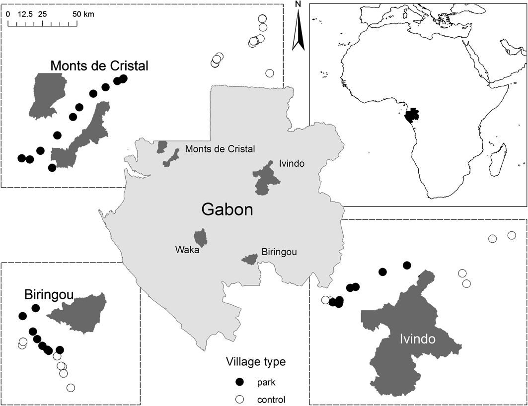
Fig. 1 The locations of the four National Parks in Gabon where the study took place (centre), and the areas and village locations in relation to three of the four National Parks (only the villages included in the intensive survey are included; see text for details). The top right figure shows the location of Gabon in West Africa.
Human population
Starting in the early colonial period at the turn of the 20th century and continuing through to independence in 1960 rural families were forcibly moved by the state to live along the few roads that connect Gabon’s towns to the capital city Libreville. Today most rural Gabonese either live in small market towns of 5,000 inhabitants or less, or in villages, often of related individuals, of 3–50 families. These village households generally employ a mixed livelihood strategy that includes farming of stable crops such as manioc, plantains, maize and yams, subsistence hunting in fields and in the forest surrounding the village, and small enterprises (sale of bushmeat, agricultural crops, palm wine, sleeping mats, brooms and other items). Labour allocation varies with the agricultural calendar and can include wage labour in logging and mining concessions.
Village selection
After initial testing and refining of survey methods in 2005–2006 we proceeded in three stages. Firstly, we conducted a participatory assessment of resource use to determine whether or not village residents presently or historically used or had claims over natural resources now within the boundary of the National Park. Villages with prior or present use or claims were designated park villages (n = 72, distance from park boundary 2–37 km, median = 16 km), those without were designated non-park, i.e. control villages (n = 45, distance from park boundary 20–128 km, median = 60 km). We attempted to match as closely as possible the number of park and control villages (Table 1) but this was not always possible given a low population density and the spatial distribution of villages in relation to park boundaries.
Table 1 Number of villages/households at the four National Park study sites (Fig. 1) included in the extensive and intensive surveys (see text for details). Not all households provided information on each of the indicators, leading to variable sample sizes.
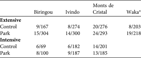
* Study villages at Waka National Park could not be included in the intensive survey because roads to this part of the country became impassable at that time
Secondly, we conducted an extensive survey of all park and control households to capture information on household composition, education, health, income and wealth (assessed with a standard basket of goods; see below). Thirdly, we conducted an intensive survey of a subset of park and control households at three sites (n = 56 villages; Table 1, Fig. 1) to capture information on consumption of wild, cultivated and manufactured goods. To account for seasonal changes in consumption patterns we conducted two separate intensive surveys: February–May 2006 (dry season) and September–December 2006 (wet season). Two researchers spent 1 week in each village and conducted household interviews on days 1, 3 and 5 for 50% of households, and on days 2, 4, and 6 for the remaining 50%. On each visit the interviewers asked the adult male and female heads of household to recall all goods consumed (i.e. brought over the threshold of the house) during the previous 48 hours. Prior surveys on bushmeat consumption demonstrated that subjects are rarely willing to divulge where they hunt or set traps, probably because of fear of prosecution. Therefore, we chose simply to ask whether the goods consumed came from forests, agricultural fields or fallows, or from shops and markets.
Village level information
For each village we recorded name, geographical location, number of households, market access, travel time to social services, access to electricity and whether village members participate in community work. We analysed land cover in a 5-km radius around each village using GlobCover v. 2.2 (ESA, 2008). GlobCover provides gridded global land cover at a resolution of 300 m (MERIS Full Resolution Level 1B product), and covers December 2004–June 2006. Land cover classes are regionally-tuned and defined according to the UN Land Cover Classification System (FAO, 2005). All spatial analyses were carried out with ArcGIS v. 9.3.1 (ESRI, Redlands, USA).
Demography and well-being
We gathered demographic information (age, gender, years of education and ethnicity) for all household residents. Residents were defined as all individuals sleeping in the residence during the 7 days prior to the survey. We gathered anthropometric information (body-mass index (BMI; weight/(height)2), percentage body fat and mid upper-arm circumference) for all household residents > 1 year of age as a proxy for short-term health. All residents were asked how often they had suffered from fever, diarrhoea and the common cold in the previous month. In addition, the head of each household was asked to provide a self-assessment of their nutritional well-being as the number of days in the previous month they had not eaten anything. Community trust was assessed by asking participants whether they would trust a neighbour to look after their house when they had to leave the village, to look after their money, or whether a machete left outside overnight would still be there in the morning.
We followed the guidelines for protection of human subjects as outlined by the Belmont Report (The National Commission for the Protection of Human Subjects of Biomedical and Behavioral Research, 1979) and data collection protocols were reviewed and authorized by the Boston College Institutional Review Board. All researchers were required to complete an online Human Subjects Protection certification course and participated in a 2-week training programme on collecting anthropometric measurements. Potential subjects were given details, in their natal language, about the study and informed that it was a university research project to determine how national parks affect the lives of people in Gabon who live near them. We informed potential subjects that if they participated they would remain anonymous and their identity would never be revealed at any time during the study or in any reports or publications arising from the study. Potential subjects were also informed that they had the right to refuse to answer any question or to end their participation in the study at any time. Prior to each data collection event subjects were reminded of the purpose of the study and again asked if they still wished to participate. We asked parents’ permission to collect anthropometric measurements of their children under the age of five. Information about children’s health measures was provided to parents only. No remuneration was offered to participants.
Income
Household wealth was assessed from the total value of a standard basket of 22 assets owned by any household member. We chose the basket of assets to include items that span a broad range of values and thus were likely to be owned by households that differ widely in wealth: cooking equipment, firearms, beds, mattresses, lamps, watches, clocks, refrigerators, freezers, music players, televisions, mobile phones, electric fans, air conditioners and vehicles. All values were recorded in XAF and reported in purchasing power parity USD (PPP$). We used the PPP conversion factor for private consumption in 2005, which was 443.7 (World Bank, 2008). We used the current village price for each asset and did not impute a depreciated value based on the age of each owned asset, as this has been shown (Demmer & Overman, Reference Demmer and Overman2001) not to significantly influence wealth assessment and considerably reduces the time to gather asset data, thus minimizing subject fatigue and data error.
To estimate transitory income all household residents were asked to recall the amount of income generated during the previous month from salaries, wages, bonuses, pensions, remittances, and revenue from commercial enterprises and the sale of forest goods. Value of annual crops was assessed by asking subjects to recall the total sales price of each crop that is only harvested and sold once per year (e.g. coffee, cacao, peanuts). We divided income into categories that reflected income ranges and let each subject privately point to the category their respective incomes would fall into.
Measuring consumption
Heads of households were asked to recall all produce, natural resources and manufactured goods consumed (purchased, hunted, caught or otherwise obtained) during the 48 hours prior to the survey by all members of the household. For each consumed item, heads of households provided an actual or estimated value in XAF as well as the number of units consumed. For items produced by the household (e.g. bushmeat trapped or hunted) we estimated its value by asking interviewees the price they would have sold it for, or the quantity of a good with a known price (e.g. 1 kg of sugar) they would trade if for.
To obtain an adequate measure of animal protein consumption that was not influenced by variation in market value we transformed all protein consumption (except tinned fish) into kg. As the majority of protein consumption was based on units other than kg, we estimated the weight for each item in one of four ways: (1) For some frequently used units we obtained mean weights from a previous consumption study among urban and rural villages in Gabon (Wilkie et al., Reference Wilkie, Starkey, Abernethy, Effa, Telfer and Godoy2005); (2) When the weight per unit was not known we used the price of whole specimens to estimate weight consumed as (value consumed) * (mean weight whole) / (mean price whole); (3) When price data for whole animals were not available for the village in which they were consumed (15% of all cases) we used the mean price for the whole animal calculated across all villages; (4) If a mean weight of the whole animal could not be obtained from our records we used mean weights in the literature for an adult of that species, if available. For 62 records weight could not be calculated by these methods and we excluded those records from analyses. We excluded an additional 60 records because the respective households were only surveyed on 1 or 2 days. The final dataset included 3,633 consumption records.
Statistical analyses
Consumption and income measures were expressed per adult male equivalent (AME) to control for different demographic compositions of households (Deaton, Reference Deaton1997). Conversion into AME was based on estimated daily food energy requirements (kcal day-1) for different ages and genders (James & Schofield, Reference James and Schofield1990). Most livelihood measures were greatly skewed and many zeros prevented transformation to normality. We therefore used Mann–Whitney U tests to evaluate differences between park and control households. If parks themselves had an effect on livelihoods we would expect some of our indicators to correlate with distance to the nearest park boundary, rather than the designation of park vs control that ignores intra-group variation in spatial separation from the parks. To test this hypothesis we constructed generalized linear models with distance to nearest park boundary as a covariate. To account for between-site variation in dependent variables we also entered study site and its interaction with distance as fixed effects. We modelled dependent variables using a log-link function. To account for correlation between independent factors and assess the relative importance of different measures to distinguish between park and control households we used binary logistic regression with park/control as the dependent variable, and the following predictor variables entered through a forward likelihood ratio selection criterion: distance to park, income, wealth, education, household size (AME), total consumption (XAF), consumption of protein except canned meat and fish (kg), consumption of game meat, chicken, livestock and fish (kg), consumption of vegetables (XAF), consumption of non-food (XAF), mean BMI, and distance to market (km). Significance levels for all statistical tests were set to α = 0.05. All tests were two-tailed and performed with PASW Statistics v. 17 (SPSS Inc., Chicago, USA).
Results
Community indicators
Park villages were significantly smaller than control villages (mean 109 ± SE 10 vs 155 ± SE 16 inhabitants, respectively; Z = -2.5, P = 0.011, n = 45 vs 72 control and park villages). Distance to markets and larger towns (in hours) was not different between control and park villages (Table 2; markets: Z = 1.2, P = 0.22; larger towns: Z = 1.3, P = 0.21; see Table for sample sizes). Control villages were significantly further away from park boundaries than park villages (median = 60 vs 16 km for control and park villages, respectively; Z = -8.7, P < 0.001) but distance was more variable among control than park villages (Table 2). Control villages were further from the nearest dispensary than park villages (median = 1.0 vs 0.5 h; Z =-2, P = 0.04) but did not differ in travel time to the nearest pharmacy (median = 1.5 vs 1.0 h; Z = 0.1, P = 0.94) or hospital (median = 1. 5 vs 1.25 h; Z = 0, P = 1.00).
Table 2 Selected village and livelihood measures (mean ± SE (n)) among control and park villages/households included in the extensive survey (see text for details), and significance levels for the comparison of both groups (Mann−Whitney U tests).
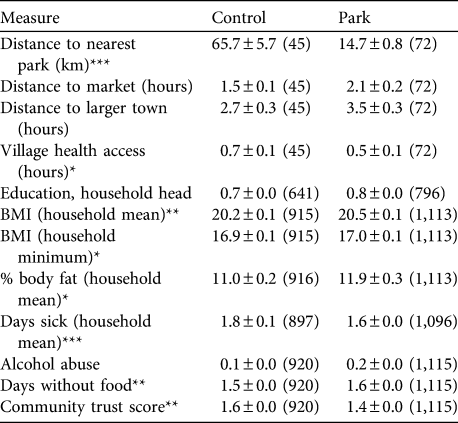
*P < 0.05; **P < 0.01; ***P < 0.001
The median level of trust was 2 in control households (i.e. they answered yes to two of the three trust-related questions) and 1 in park households (Z = -3.1, P = 0.002, n = 922 vs 1,137 control and park households, respectively). However, the only difference between park and control households appeared in response to the question about trusting a neighbour with money; members of control households were more likely to show trust than park households (Z = -5.4, P < 0.001, n = 1,338 vs 1,774 participants in control and park households, respectively).
Park and control villages selected for the intensive survey differed significantly in the area covered by different vegetation types within a 5 km radius. The area covered by closed rainforest (> 40% cover of main tree layer) and seasonally flooded forest was greater around park than control villages (closed rainforest: 69.1 ± SE 3.0%, n = 26 vs 82.9 ± SE 1.9%, n = 30 control and park villages, respectively, Z = -3.6, P < 0.001; seasonally flooded rainforest: 2.0 ± SE 0.5% vs 6.9 ± SE 0.9%, Z = -3.5, P < 0.001) and closed to open rainforest (> 15% cover of main tree layer) and forest/crop land mosaics were more common around control villages (closed to open rainforest: 16.8 ± SE 1.6% vs 7.1 ± SE 0.8%, Z = -4.3, P < 0.001; forest/crop land mosaic: 9.9 ± SE 1.4 vs 2.8 ± SE 0.9%, Z = -3.7, P < 0.001).
Household indicators
Park households earned significantly less income than control households (PPP$ 150.3 ± SE 9.5 vs 220.9 ± SE 14.9 for park and control households, respectively; Z = -6.23, P < 0.001, n = 1,137). Different directions of effects, however, were observed with specific income sources (Table 3). Control households sold significantly more mineral and cultivated goods than park households but there was no difference in income from sale of wild animal and plant products. Nevertheless, park households earned a greater proportion of sales income from wild products than control households (25.3 ± SE 1.5% vs 17.4 ± SE 1.3% of all income, Z = -2.9, P = 0.003, n = 657 vs 597 park and control households, respectively).
Table 3 Mean ± SE total monthly income (purchasing power parity USD; see text for details) from various sources in control and park households and significance levels for the comparison of both groups (Mann−Whitney U tests).
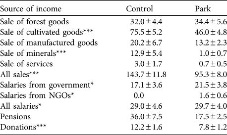
*P < 0.05; ***P < 0.001
Total income from employment was greater in control than park households, mostly because of a difference in salary from private entities. Park households received significantly more income from the state and NGOs than control households but comparatively fewer donations. Although there was a significant difference in household size between park and control when expressed as AME (park: 5.0 ± SE 0.2, n = 913; control: 5.7 ± SE 0.2, n = 705; Z = -4.3, P < 0.001), expressing income per AME did not change the income differences from sales. However, salaries per AME did not differ between park and control households, regardless of the source. Wealth, as estimated by valuing a standard basket of assets for each household, did not differ between park and control households (park: PPP$ 1,323.6 ± SE 68.8, n = 887 vs control: PPP$ 1,168.6 ± SE 44.5, n = 693; Z = -0.51, P = 0.612).
Level of education of the household head did not differ between park and control households (Table 2; Z = 0.7, P = 0.49). Overall, 47.2% of household heads had no education, 34% completed school to fifth grade (10–11 years), 15.9% up to ninth grade (14–15 years), and only 3% had higher levels of education (median: fifth grade).
Health indicators
The median BMI of park household members was slightly greater than that for control households, regardless of whether we used the household means or minima in the analysis (Table 2). The difference was small, however (household means: median = 20, range 13.7–48.3 vs 20.3, range 7.1–40.1, for control and park households, respectively; Z = 2.8, P = 0.005; see Table 2 for sample sizes). Members of park households had a slightly greater percentage body fat than those of control households (Table 2; Z = 2.1, P = 0.033) and the heads of control households reported slightly fewer days per month without consuming any food compared to park households (Z = 3.2, P = 0.001).
Members of control households reported more sick days in the previous month than park households (Table 2; Z = -4.0, P < 0.001). For all of the most common illnesses examined, members of control households reported slightly more cases over the previous month than members of park households (fever: 0.74 ± SE 0.02 vs 0.66 ±SE 0.01 times; Z = -4.5, P < 0.001; diarrhoea: 0.36 ± SE 0.01 vs 0.26 ± SE 0.0 times; Z = -6.6, P < 0.001; common cold: 0.64 ± SE 0.01 vs 0.57 ± SE 0.01 times; Z = -4.1, P < 0.001; n = 3,959 vs 4,916 members of control and park households, respectively). The median number of times with illnesses per month was zero for both park and control households.
Consumption
Among the main protein sources game meat was most commonly consumed. Mean household consumption was 9.4 ± SE 0.7 kg of game meat per month per AME, with no difference between park and control households (Z = -1.0, P = 0.92, n = 381 vs 376 control and park households, respectively). Wild caught fish and domestic chicken and livestock were consumed more in park than control households but the difference was only significant for chicken consumption (fish: 1.1 ± SE 0.1 vs 1.4 ± SE 0.1 kg month-1 AME-1 for control and park households, respectively, Z = -0.2, P = 0.84; chicken: 0.2 ± SE 0.0 vs 0.5 ± SE 0.1 kg month-1 AME-1, Z = -5.0, P < 0.001; livestock: 0.07 ± SE 0.01 vs 0.12 ± SE 0.03 kg month-1 AME-1, Z = -0.8, P =0.4).
Consumption of vegetables and fruits, regardless of source, did not differ significantly between park and control households. Village medians for consumption of fruits and vegetables purchased from stores were higher in park than control villages (PPP$ 2.7 vs 1.4 month-1 AME-1, Z = -2.9, P = 0.003), as were the village medians for meat purchased from stores (PPP$ 2.7 vs 1.8 month-1 AME-1, n = 498 and 485 for park and control households, respectively, Z = -4.0, P < 0.001). There were no differences between park and control households in the consumption of non-food items.
Do livelihood measures vary with distance to park?
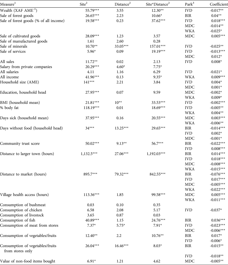
Results of the generalized linear models controlling for distance to the nearest park boundary are provided in Table 4. The majority of livelihood measures differed between sites, and interactions between site and distance to parks were common. Only consumption of animal protein (in kg) and vegetables/fruits purchased from stores (in XAF) showed a consistent and significant decline with greater distance from park boundaries. This result indicates that variation in most livelihood measures was more influenced by site-specific idiosyncrasies than a consistent effect of distance to parks.
Table 4 Results of generalized linear models investigating the effects of park and distance to nearest park boundary on variation in livelihood measures across villages. Site evaluates differences between parks, Distance evaluates the effect of distance to park boundaries, and SiteFootnote *Distance evaluates the interaction between Site and Distance. Park identifies parks with significant distance effects, and Coefficient gives the effect sizes and directions.
*P < 0.05, **P < 0.01, ***P < 0.001
1 Income from sales and salaries are XAF month-1 AME-1, consumption measures are kg month-1 AME-1 for bushmeat, chicken, livestock and fish, and XAF month-1 AME-1 for all other consumption
2 Values given are Wald χ2 statistic
3 BIR, Biringou; IVD, Ivindo; MDC, Monts de Cristal; WKA, Waka
What factors best distinguish between park and control households?
In our multivariate logistic models distance to park boundary was the single best predictor for classifying households into park and control (94.5% of all households classified correctly by the model). However, as this solution was trivial we removed that predictor to examine effects of other factors of interest. The best model, with a predictive power of 59.4% (44.7% for control households, 69.6% of park households), included household size (odds ratio =0.96) and consumption of chicken (odds ratio = 1.37). Thus, household sizes were smaller in park than control villages, and households in park villages consumed greater quantities of chicken. The low predictive power of the model suggests, however, that none of the livelihood measures differed greatly and consistently between park and control households. To reduce random variability among households and improve model fits, we used village means in a separate binary logistic regression. Results were identical to the household level analysis, with household size (odds ratio = 0.76) and consumption of chicken (odds ratio = 13.85) being the most useful factors distinguishing between park and control (73.1 and 70% of villages, respectively, classified correctly).
Discussion
Our goal was to assess whether communities with traditional and ongoing claims to resources within the boundaries of national parks differed in livelihood measures from control communities that do not use or claim access to these same resources. Our results show that there were differences between these communities in land cover and in income generating activities. Park households relied to a greater extent on wild animal and plant products, and control households obtained relatively more income from agriculture. However, although park households had significantly lower overall income than control households from the sale of goods, indicators of welfare such as consumption, access to health care, education and wealth did not differ significantly between the two groups. In particular, households in park and control villages received their main animal protein from wildlife, similar to what has been reported for other parts of Gabon (Wilkie & Carpenter, Reference Wilkie and Carpenter1999; van Vliet & Nasi, Reference van Vliet and Nasi2008; Blaney et al., Reference Blaney, Beaudry and Latham2009) and elsewhere (Lahm, Reference Lahm, Hladik, Hladik, Linares, Pagezy, Semple and Hadley1993). Given the greater proportion of land covered with intact forest around park villages, the greater reliance on forest resources among park households was not unexpected. This suggests that livelihoods of communities with traditional claims to park resources may be more likely to suffer if conservation and management practices restrict access to, and use of, forest products (McElwee, Reference McElwee2010) and do not provide alternative income sources and protein supplies (Loibooki et al., Reference Loibooki, Hofer, Campbell and East2002; Robinson & Bennett, Reference Robinson and Bennett2004; Ohl-Schacherer et al., Reference Ohl-Schacherer, Shepard, Kaplan, Peres, Levi and Yu2007).
There appeared to be a small but significant difference in welfare measures related to food stability and incidence of diseases. Heads of households in park villages did not consume food on twice as many days as heads of households in control villages. As control households rely more on cultivated foods they may experience less volatility in food supply than park households that rely more on wild food resources (van Vliet & Nasi, Reference van Vliet and Nasi2008). The difference between park and control households was small, however, and its relevance as an indicator of nutritional status or welfare is uncertain. The finding that control households were more likely to suffer from common infectious illnesses could be related to the larger size of control villages, because larger aggregations of hosts may better sustain populations of disease vectors (Anderson & May, Reference Anderson and May1979; Lindenfors et al., Reference Lindenfors, Nunn, Jones, Cunningham, Sechrest and Gittleman2007).
In general, previous empirical assessments of the relationship between human welfare and protected areas have found evidence for both positive and negative associations, supporting the notion that any effects tend to be highly localized and specific to each protected area. Furthermore, we still know little about the long-term effects of protected areas on human welfare because longitudinal data on welfare indicators are generally not available for many developing nations, particularly in Africa. Analysis of the long-term influences of protected areas on human welfare using historical and current indicators of welfare in Costa Rica and Thailand (Andam et al., Reference Andam, Ferraro, Sims, Healy and Holland2010), two relatively well-developed countries compared to Sub-Saharan Africa, indicated that protected areas improved human livelihoods after confounding variables were controlled for, although imperfect measures, great variability, and the unplanned nature of the study left some uncertainty about true cause and effect relationships.
Although our comparison of park and control households revealed no overall systematic difference in welfare measures despite variation in land use and income, site-specific conditions lead to significant variation across the study sites for almost all our livelihood measures. For example, income differences between park and control communities were most apparent at Waka National Park but not significantly different at other sites (Fig. 2). Similarly, consumption of vegetables and fruits was significantly lower in park than control villages at Biringou, higher in park than control villages at Ivindo, and not significantly different at Monts de Cristal (Fig. 3). Such site-to-site variation in livelihood measures probably results from existing variation in environmental, historical, social and economic factors (Fa et al., Reference Fa, Juste, Burn and Broad2002, Reference Fa, Albrechtsen, Johnson and Macdonald2009). Understanding the drivers of these differences has implications for management and poverty intervention schemes, as well as the future assessments of livelihood impacts of establishing and managing protected areas. This site-specific variation in the difference between park and control households also lends further support to the idea that proximity to park resources itself was not the primary cause of the variation we observed but that these differences are caused by local idiosyncrasies at each site, which remain to be explored.
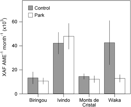
Fig. 2 Site-specific variation in household income from all sources (mean ± 95% confidence interval) for households in control and park villages at the four National Park study sites (Fig. 1).
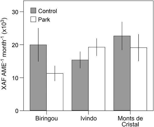
Fig. 3 Site-specific variation in consumption of fruits and vegetables (mean ± 95% CI) for households in control and park villages at three of the four National Park study sites (Fig. 1).
As this study evaluated variation in livelihood measures before the implementation of laws governing the newly established parks, we cannot make inferences about the role of these parks in influencing human welfare. We can, however, assess the influence of being close to the natural resources that are protected in these parks, and found that the variation in resource access between control and park villages was not sufficient to cause major differences in human livelihood measures. A future survey (Wilkie et al., Reference Wilkie, Morelli, Demmer, Starkey, Telfer and Steil2006), to be conducted within the next 5-10 years, will allow conclusions to be drawn about the direct influence of park management practices on human welfare and contribute to the ongoing debate on livelihood impacts of establishing protected areas as a means for sustainable biodiversity conservation.
Acknowledgements
The Parks and People research in Gabon is supported with start-up funding from the John D. and Catherine T. MacArthur Foundation, and is being undertaken by Boston College in collaboration with the Conseil National des Parcs Nationaux of Gabon and the Wildlife Conservation Society. We acknowledge the work of our team of Gabonese social scientists: Estelle Bouanga, Guy-Modeste Mengue, Franck Mouleka and Yves-Eric Pangou.
Biographical sketches
Steffen Foerster is a behavioural ecologist with research interests in wildlife conservation and management. David Wilkie is an ecologist and Gilda Morelli is a cultural and developmental psychologist; both have worked with hunter-gatherers for over 20 years and are interested in the economic and social factors that drive natural resource use. Josefien Demmer is an ecologist interested in human ecology. Malcolm Starkey is a geographer, Paul Telfer is a primatologist and Matthew Steil is a conservation biologist; all continue to work in Central Africa helping government agencies, private sector companies and local communities manage natural resources sustainably and conserve the region’s spectacular wildlife.

