


1. Introduction
Nowadays, reliability is recognized as one of the most important and dynamic research fields (e.g., [Reference Xie, Dai and Poh36]). Its interdisciplinary nature and ubiquitous presence in applied domains are at the roots of the continuously expanding literature. In its basic form, reliability is defined as the probability of a system performing without failure for a given period of time. In some circumstances, it is common to consider a system as formed by multiple components, say N. Each component can fail according to specific probabilistic rules. The failure of the entire system arrives when a given number of components, say K of them, are in the fault state. This type of system is known as K-out-of-N systems (see, e.g., [Reference Boland and Proschan2, Reference Goliforushani, Xie and Balakrishnan13, Reference Linton and Saw24, Reference Vishnevsky, Selvamuthu, Rykov, Kozyrev, Ivanova and Krishnamoorthy34]) and frequently finds a description in terms of multi-state models. The latter found extensive use in reliability both in Markov [Reference Koutras and Maravelakis19] and semi-Markov cases [Reference D’Amico10, Reference Limnios23] and in their generalizations [Reference Cui, Yi and Jiang8, Reference D’Amico9, Reference D’Amico, Petroni and Prattico11].
Different modifications and extensions of this basic framework are considered in the literature. A non-exhaustive list includes systems with common-cause failures as a representative dependent failure into system analysis (see, e.g., [Reference Yuge, Maruyama and Yanagi37]); systems with two types of components characterized by different failure rates (see, e.g., [Reference Zhang, Xie and Horigome38]); systems with two distinct failure modes where failed components are repaired by a single repair facility instantly or may enter a waiting phase and try again to be repaired after some time [Reference Li, Hu, Wang and Kang22]; weighted systems in which the components have an asymmetrical impact on the system’s lifetime (see, e.g., [Reference Rahmani, Izadi and Khaledi27, Reference Zhang, Ding and Zhao39]); sequential K-out-of-N system that takes into account that failures of components possibly affect remaining ones [Reference Cramer and Kamps7] and consecutive K-out-of-N system which fails if and only if at least K consecutive components are failed [Reference Gao, Cui and Chen12, Reference Huang, Zuo and Fang15]. Increasing interest was shown toward repairable systems, in which there was the possibility to repair the fault components using a repair facility [Reference Rykov30].
Exotic properties for a K-out-of-N system are investigated in [Reference Ito, Zhao and Nakagawa16] who studied the reliability and preventive replacement problems when K is considered a random variable. Asadi [Reference Asadi1] studied the phase transition problem in high-dimensional K-out-of-N systems, which consists of the possibility that the system reliability undergoes a sharp transition when the components are independent and identical to each other.
The applications can be from different scientific domains. As a matter of example, Rykov, Sukharev, and Itkin [Reference Rykov, Sukharev and Itkin33] demonstrated possible applications to the oil and gas industry with the calculation of the reliability function and its variability with respect to component repair time distributions. Cerqueti [Reference Cerqueti4] studied a financial derivative model, which consists of a special class of barrier basket options, on the ground of K-out-of-N systems.
The majority of the research works considered exponential repair time distributions [Reference Wu, Li and Bérenguer35] or phase-type distributions [Reference Ruiz-Castro29]. Some authors considered systems with a general repair time distribution [Reference Moustafa26, Reference Rykov, Kozyrev, Filimonov and Ivanova31]. This aspect is very important as the obtained results are more general, and the models could be applied without constraints to real problems. Recent contributions by [Reference Rykov, Kozyrev, Filimonov and Ivanova31] and [Reference Rykov and Filimonov32] described the system in terms of non-Markovian multi-state models. The authors applied the Markovization method to find the reliability function of a K-out-of-N system with a general repair time distribution. They derived the system of Kolmogorov forward partial differential equations (PDEs) and provided its solution by advancing an algorithm based on the method of characteristics.
In this article, motivated by the two important contributions given in [Reference Rykov, Kozyrev, Filimonov and Ivanova31] and [Reference Rykov and Filimonov32], the underlying research stream generalizes it further. The main contribution is to advance a new repair mechanism by defining the effort rate function  $r_{J(t)}(X(t),S(X(t)))$. This function expresses the idea that the system can be repaired with different rates of effort. The latter depends on three variables: the number of fault components J(t), the time since the last repair has started X(t), and the instantaneous effort produced at that time, that is, $S(X(t))$. Moreover, the effort function $S(X(t))$ is linked to the effort rate $r_{J(t)}(X(t),S(X(t)))$ by a nonlinear differential initial value Cauchy problem. Therefore, the repair mechanism can be very flexible, allowing increasing/decreasing shape of the effort function according to the specification of the three variables and their interconnections. The proposal of the effort function as a tool to enhance the flexibility of the repair mechanism and its formal definition and analysis has never been faced before in the literature. This makes the contribution of this paper unique and at the same time generalizes previous works.
This theoretical proposal is motivated by the practical possibility in a specific system to design the repair policy such that a modulation can be implemented in order to speed up the repair of fault components by implementing a large effort or to slow down the repair chance by putting less effort into the repair. Examples of systems of this type can be represented by those requiring installed resources with limited capacity to perform repairs, and the chance of getting a repair depends on the quantity of resources used. A possible applied domain could be the one represented by small satellites [Reference Kopacz, Herschitz and Roney18]. The satellite has N batteries and works well while N − K of them are charged and working. This is an example of a K-out-of-N system with a resource (energy) that should be managed attentively in such a way that a nonworking component (one of the discharged batteries) could be repaired (charged at a sufficient level). This is only a hypothetical system that can be described according to the theoretical model that is going to be developed in this study.
The contribution of this study also has the merit of allowing a better understanding of the model advanced in [Reference Rykov, Kozyrev, Filimonov and Ivanova31]. In fact, it is realized that the model by [Reference Rykov, Kozyrev, Filimonov and Ivanova31] is obtained for a very simple and specific choice of the effort rate function that should be unitary, that is,  $r_{J(t)}(X(t),S(X(t)))=1$. Hence, in the [Reference Rykov, Kozyrev, Filimonov and Ivanova31] framework, even without mentioning it, the authors considered a unitary rate of effort function, while in our setting it can be designed as a nonlinear function whose evolution is determined according to the dynamic of a piecewise deterministic Markov process.
The more general framework gives increasing flexibility and potential in the application of the theory, but the more complex the model, the more difficult the results are. To this end, first a mathematically rigorous definition of the model is provided by advancing a set of specific assumptions. Further, a regularity result for the failure and repair counting processes is provided. The regularity result is necessary to derive a system of Kolmogorov forward PDEs for the state probabilities. This system contains, as a very particular case, the one obtained in [Reference Rykov, Kozyrev, Filimonov and Ivanova31]. It shows the intricacies between the failure mechanism, the base repair mechanism, and the modulated one. Moreover, a comparison result between the reliability functions of two K-out-of-N systems of the type studied is provided. Sufficient hypotheses for the reliability of one system to be uniformly in time greater than the reliability of the other are given. The illustration of how the theoretical results can be achieved in practical situations is provided by a numerical illustration.
This paper follows the following structure: the subsequent section will define the problem and introduce relevant notations and basic assumptions defining the model. The theoretical results are discussed in Section 3, which includes the regularity result for the involved counting processes, the Kolmogorov system of PDE for the probability densities, and the result concerning the ordering of the reliability functions. Section 4 presents numerical examples for specific cases. Finally, the article concludes with a summary in Section 5.
2. Model description
Let us consider a model of a homogeneous, repairable K-out-of-N system in which the failed components are repaired by a single repair facility. According to the research line developed in [Reference Rykov, Kozyrev, Filimonov and Ivanova31, Reference Rykov and Filimonov32], the model explaining the failure and repair mechanisms is presented. The former coincides with the one formulated by [Reference Rykov, Kozyrev, Filimonov and Ivanova31] while the latter will differ greatly, being much more general and flexible.
2.1. The failure mechanism
A system of N components is considered that fail following a Poisson process with intensity α. Let us denote by  $j\in \{0,1,\ldots,K-1\}$ the number of fault components. Then, the system’s failure intensity is given by
 \begin{equation}
\lambda_{j}=(N-j)\cdot \alpha .
\end{equation}
\begin{equation}
\lambda_{j}=(N-j)\cdot \alpha .
\end{equation}Evidently, the lower the number of fault components, the higher the chance to experience the default of one component among the working ones.
It is worth noticing that the Poisson process of failure considers the case when flow intensity is a time-changing value depending on the number of fault components. Indeed, the overall fault intensity at time t is supposed to randomly evolve according to the next equation:
 \begin{equation}
\lambda(t)=(N-J(t))\cdot \alpha .
\end{equation}
\begin{equation}
\lambda(t)=(N-J(t))\cdot \alpha .
\end{equation} Equation (2) means that failure events occur at an average rate of  $\lambda(t)$ per unit time, which is variable as modulated by the process $\{J(t), t \geq 0\}$.
Assumption F1 (The Failure Mechanism)
The Poisson process intensity is finite at any time t, that is,  $\alpha \lt +\infty$.
Assumption F1 avoids the simultaneous occurrence of faults, which is a rather unrealistic scenario in many practical systems of interest.
2.2. The repair mechanism
The considered system can be repaired with the use of a single repair facility, which repairs the failed components according to the following probabilistic rules.
Assumption R1 (The Base Repair Mechanism)
The random variables describing the repair times of the failed components are independent and identically distributed according to a general cumulative distribution function (CDF) B(t). It is assumed that B(t) is absolutely continuous with the probability density function (PDF) b(t) [Reference Castañeda, Arunachalam and Dharmaraja3].
Assumption R1 is identical to that advanced in [Reference Rykov and Filimonov32]. It is already a general assumption that does not depend on the memoryless property of the exponential distribution of the repair times [Reference Kumar, Gopi, Harikeerthana, Gupta, Gaur, Krolczyk and Wu20, Reference Wu, Li and Bérenguer35] or a mixture of exponentials.
Remark 2.1. Assumption R1 alone is not sufficient for the scope of this work, as an absolutely continuous distribution can have an unbounded failure rate, which means that the failure rate h(t) can approach infinity as t approaches a certain value. The next example illustrates this fact. Consider a random variable X distributed according to a Weibull distribution with shape parameter k < 1 and scale parameter λ. The hazard function h(t) is given by:
 \begin{equation*}
h(t) = \frac{f(t)}{1 - F(t)},
\end{equation*}
\begin{equation*}
h(t) = \frac{f(t)}{1 - F(t)},
\end{equation*}where
 \begin{equation*} f(t; \lambda, k) = \begin{cases}
\frac{k}{\lambda} \left(\frac{t}{\lambda}\right)^{k-1} e^{-(t/\lambda)^k} & t \ge 0 \\
0 & t \lt 0
\end{cases} \end{equation*}
\begin{equation*} f(t; \lambda, k) = \begin{cases}
\frac{k}{\lambda} \left(\frac{t}{\lambda}\right)^{k-1} e^{-(t/\lambda)^k} & t \ge 0 \\
0 & t \lt 0
\end{cases} \end{equation*}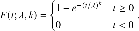 \begin{equation*} F(t; \lambda, k) = \begin{cases}
1 - e^{-(t/\lambda)^k} & t \ge 0 \\
0 & t \lt 0
\end{cases}. \end{equation*}
\begin{equation*} F(t; \lambda, k) = \begin{cases}
1 - e^{-(t/\lambda)^k} & t \ge 0 \\
0 & t \lt 0
\end{cases}. \end{equation*}Hence,
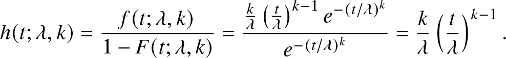 \begin{equation*} h(t; \lambda, k) = \frac{f(t; \lambda, k)}{1 - F(t; \lambda, k)} = \frac{\frac{k}{\lambda} \left(\frac{t}{\lambda}\right)^{k-1} e^{-(t/\lambda)^k}}{e^{-(t/\lambda)^k}} = \frac{k}{\lambda} \left(\frac{t}{\lambda}\right)^{k-1}. \end{equation*}
 As t → 0, if  $ 0 \lt k \lt 1 $, the hazard function $ h(t; \lambda, k) $ becomes unbounded, approaching infinity.
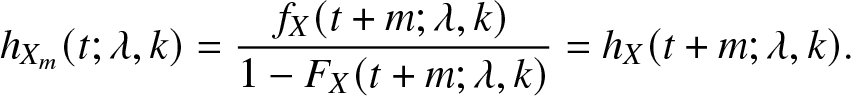
The same argument applies to any random variable  $X_{m}:=X-m$ for a positive real value of m. Immediately, we have that its repair rate is
 \begin{equation*}
h_{X_{m}}(t; \lambda, k) = \frac{f_{X}(t+m; \lambda, k)}{1 - F_{X}(t+m; \lambda, k)} = h_{X}(t+m; \lambda, k).
\end{equation*}
\begin{equation*}
h_{X_{m}}(t; \lambda, k) = \frac{f_{X}(t+m; \lambda, k)}{1 - F_{X}(t+m; \lambda, k)} = h_{X}(t+m; \lambda, k).
\end{equation*}Therefore, the random variable Xm has an unbounded repair rate in any neighborhood of m. Therefore, an absolutely continuous distribution can indeed have an unbounded failure rate, where the hazard function can grow without any bound as t approaches certain values depending on the parameters of the distribution.
This example also extends its validity to more complex settings where mixtures of Weibull distributions are considered. The mixture approach is very powerful for fitting failure time data [Reference Razali and Al-Wakeel28] even in reliability studies.
For our scope, it is necessary to introduce an additional assumption about the probability distribution of the repair times, avoiding the unboundedness of the repair rate function.
Assumption R2 (Repair Rate Function)
The CDF B(t) has uniformly bounded repair rates over compact sets, that is, the repair rate function  $\beta(x):=\frac{b(x)}{1-B(x)}$ satisfies the following condition:
 \begin{equation}
\forall L\in \mathbb{R}, \exists M_{L}\in \mathbb{R}\,\, \text{such that}\,\, \sup_{x\in [0,L]}\beta(x) \lt M_{L}\,.
\end{equation}
\begin{equation}
\forall L\in \mathbb{R}, \exists M_{L}\in \mathbb{R}\,\, \text{such that}\,\, \sup_{x\in [0,L]}\beta(x) \lt M_{L}\,.
\end{equation}This assumption is necessary to avoid the possibility of unbounded repair rates over a compact set, which may cause instantaneous repairs and then irregular behavior of the system.
Now, the most important assumption that characterizes the presented model is advanced.
Assumption R3 (The Modulated Repair Mechanism)
Let  $\{T_{n}\}_{n\in \mathbb{N}}$ be the sequence of increasing times when the repair of any fault component is completed. Set $T_{0}=0$ to denote a system starting with all of the N components in working condition. Let us introduce an auxiliary nonnegative real-valued random process $\{S(t), t\geq 0\}$ called the effort function and defined as $S(t):=S(X(t))$, where X(t) is the process denoting the elapsed repair time of the component under repair at time t. The main reason for introducing this function is to provide a flexible tool for speeding up or slowing down the repair time of the fault component according to the system’s status.
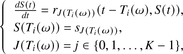
For every time  $t\in [T_{i}(\omega),T_{i+1}(\omega))$, the effort function process evolves according to the next Cauchy initial value problem:
 \begin{equation}
\left\{
\begin{array}{l}
\frac{dS(t)}{dt}= r_{J(T_{i}(\omega))}(t-T_{i}(\omega),S(t)),\\
S(T_{i}(\omega))=s_{J(T_{i}(\omega))},\\
J(T_{i}(\omega))=j\in\{0,1,\ldots,K-1\},
\end{array}
\right.
\end{equation}
\begin{equation}
\left\{
\begin{array}{l}
\frac{dS(t)}{dt}= r_{J(T_{i}(\omega))}(t-T_{i}(\omega),S(t)),\\
S(T_{i}(\omega))=s_{J(T_{i}(\omega))},\\
J(T_{i}(\omega))=j\in\{0,1,\ldots,K-1\},
\end{array}
\right.
\end{equation}where the deterministic function
 \begin{equation}
r:\{0,1,\ldots,K-1\}\times \mathbb{R}_{+}\times \mathbb{R}_{+}\rightarrow \mathbb{R},
\end{equation}
\begin{equation}
r:\{0,1,\ldots,K-1\}\times \mathbb{R}_{+}\times \mathbb{R}_{+}\rightarrow \mathbb{R},
\end{equation} is called the effort rate function. It is assumed that,  $r_{0}(\cdot,\cdot)=0$ and $s_{0}=0$ so that the effort process S(t) remains zero when the system works perfectly and no effort is made to repair it because no component has failed.
The dynamical evolution of the effort process  $S(X(t))$ is very general and can include cases in which the maximum effort is made to repair the system whenever it experiences a few or numerous failures based on the value of J(t). Hence, the reliability engineer has the opportunity to modify the reliability of the system by designing the effort function according to the objective to be achieved.
The Cauchy problem (4) describes a very flexible repair mechanism. Indeed, as an example, let us assume that at the time  $T_{i}=t_{i}$ the system has two fault components, hence $J(t_{i})=2$. Time $T_{i}=t_{i}$ is a time of completion of a repair, and then the time since the last repair is zero ( $X(t_{i})=0$). The system starts to repair one of the two failed components with an initial effort $S(t_{i})=s_{2}$ depending on the number of fault components and produces an effort variable in time according to the Ordinary Differential Equation (ODE)
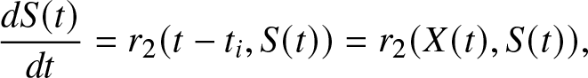 \begin{equation}
\frac{dS(t)}{dt}= r_{2}(t-t_{i},S(t))=r_{2}(X(t),S(t)),
\end{equation}
\begin{equation}
\frac{dS(t)}{dt}= r_{2}(t-t_{i},S(t))=r_{2}(X(t),S(t)),
\end{equation}for any time t before the next repair is complete.
It is important for our purpose that the Cauchy problem (4) admits a unique solution in the time interval  $[T_{i}(\omega),T_{i+1}(\omega))$. To ensure this property, further assumptions on the effort rate function need to be imposed.
Assumption R4 (Lipschitz Condition)
The effort rate function is global uniform Lipschitz continuous, that is,  $\exists L:E\rightarrow \mathbb{R}$ such that
 \begin{equation*}
\forall x, z, w,\,\,\,\,|r_{i}(x,z)-r_{i}(x,w)|\leq L(i) \cdot |z-w|\,.
\end{equation*}
\begin{equation*}
\forall x, z, w,\,\,\,\,|r_{i}(x,z)-r_{i}(x,w)|\leq L(i) \cdot |z-w|\,.
\end{equation*} Under this assumption, it is well-known that the Cauchy problem (4) has a global solution defined on the interval  $[T_{i}(\omega),T_{i+1}(\omega)]$ which will be denoted by $\xi_{j,s_{j}}(x)$, see, for example, [Reference Chiquet and Limnios5] in relation to a different problem involving the study of the transition function of a piecewise deterministic Markov process with application to reliability.
Assumption R5 (The Repair Time Distribution)
It is assumed that each random variable  $T_{n+1}$ conditionally on $J(T_{n})=j$ is generated according to a probability distribution having a conditional repair density $\beta_{J(T_{n})}(x)$ depending on the number of fault components and on the time elapsed since the last repair x according to the base CDF B(t) modulated by the effort function, that is,
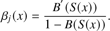 \begin{equation}
\beta_{j}(x)=\frac{B^{'}(S(x))}{1-B(S(x))}.
\end{equation}
\begin{equation}
\beta_{j}(x)=\frac{B^{'}(S(x))}{1-B(S(x))}.
\end{equation}It is simple to realize that
 \begin{equation}
\beta_{j}(x)=\frac{B^{'}(\xi_{j,s_{j}}(x))\cdot \xi_{j,s_{j}}^{'}(x)}{1-B(\xi_{j,s_{j}}(x))}=\beta(\xi_{j,s_{j}}(x))\cdot \xi_{j,s_{j}}^{'}(x)= \beta(\xi_{j,s_{j}}(x))\cdot r_{j}(x,\xi_{j,s_{j}}(x)).
\end{equation}
\begin{equation}
\beta_{j}(x)=\frac{B^{'}(\xi_{j,s_{j}}(x))\cdot \xi_{j,s_{j}}^{'}(x)}{1-B(\xi_{j,s_{j}}(x))}=\beta(\xi_{j,s_{j}}(x))\cdot \xi_{j,s_{j}}^{'}(x)= \beta(\xi_{j,s_{j}}(x))\cdot r_{j}(x,\xi_{j,s_{j}}(x)).
\end{equation}In our model, the conditional repair density is equal to the base conditional failure density computed at the effort value produced by the system multiplied by the rate of the effort function.
The introduction of the modulated repair mechanism also gives us the opportunity to better understand the generating idea behind the basic model developed in [Reference Rykov, Kozyrev, Filimonov and Ivanova31]. This model is generated by the simplest Cauchy problem, which consists of setting the effort rate function as
 \begin{equation}
r_{j}(x,y)=1, \,\forall j\in \{0,1,\ldots,K-1\},\,\text{and}\,\,\forall x,y\in \mathbb{R}_{+},\text{with}\,s_{j}=0.
\end{equation}
\begin{equation}
r_{j}(x,y)=1, \,\forall j\in \{0,1,\ldots,K-1\},\,\text{and}\,\,\forall x,y\in \mathbb{R}_{+},\text{with}\,s_{j}=0.
\end{equation} According to this choice, the effort function is  $S(x)=x$ which means that the effort process $S(X(t))$ coincides with the process X(t) measuring the time elapsed in the repair facility by the failed component. The consequence is that our repair mechanism collapses into the base one, which coincides with the one studied in [Reference Rykov, Kozyrev, Filimonov and Ivanova31].
The modulation mechanism introduces a new and flexible aspect related to the possibility of the engineer to modulate the effort of the repair. Mathematically, it consists of a nonlinear transformation of the time elapsed in the repair that may accelerate or decelerate the repair of the fault components and impact the reliability of the overall system. This is the strong difference between the modulation mechanism induced by the effort function and the traditional one; the latter can be seen as a static framework where the effort is given by the elapsed time in the repair facility, while the former is a dynamic environment in which the reliability engineer can specify the effort according to the status of the system and its objective in terms of the system’s reliability.
The considered K-out-of-N system can be analyzed using the Markovization method based on the introduction of supplementary variables [Reference Cox6]. The bi-dimensional Markov chain
 \begin{equation*}
Z = \{Z(t) = (J(t),X(t)), t \geq 0\},
\end{equation*}
\begin{equation*}
Z = \{Z(t) = (J(t),X(t)), t \geq 0\},
\end{equation*}describes the number of failed components at time t and the elapsed time that is spent by the repair facility for repairing the component being repaired. The state space of the process is of mixed continuous-discrete type and is defined as follows.
 \begin{equation*}
\xi = \{(0,0),(j,\mathbb{R}^+): j=\overline{1,K}\}.
\end{equation*}
\begin{equation*}
\xi = \{(0,0),(j,\mathbb{R}^+): j=\overline{1,K}\}.
\end{equation*} The state  $(0,0)$ denotes that the system has all components working well and that the time elapsed at the repair facility is zero. When the system is in state (j, x), it means that the fault components are j and one of them is under repair since x times. The symbol $\overline{1,K}$ is an abbreviated notation for the set $\{1,2,\ldots,K\}$.
The probabilistic behavior of the system can be described according to the micro-state PDF satisfying the following relation for sufficiently small dx:
 \begin{equation*}
\pi_j(t;x)dx \approx \mathbb{P}(J(t)=j,X(t)\in (x, x+dx)), ~j = \overline{1,K},
\end{equation*}
\begin{equation*}
\pi_j(t;x)dx \approx \mathbb{P}(J(t)=j,X(t)\in (x, x+dx)), ~j = \overline{1,K},
\end{equation*}and macro-state probabilities are provided by
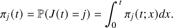 \begin{equation*}
\pi_j(t) = \mathbb{P}(J(t)=j) = \int_0^t \pi_j(t;x)dx.
\end{equation*}
\begin{equation*}
\pi_j(t) = \mathbb{P}(J(t)=j) = \int_0^t \pi_j(t;x)dx.
\end{equation*}The system’s lifetime is denoted by
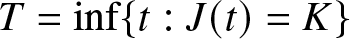 \begin{equation}
T = \inf\{t:J(t)=K\}
\end{equation}
\begin{equation}
T = \inf\{t:J(t)=K\}
\end{equation}and the system’s reliability function is defined as
 \begin{equation}
R(t) = \mathbb{P}(T \gt t)= 1- \mathbb{P}(T \leq t)= 1- \pi_K(t).
\end{equation}
\begin{equation}
R(t) = \mathbb{P}(T \gt t)= 1- \mathbb{P}(T \leq t)= 1- \pi_K(t).
\end{equation} Therefore, the reliability of the system  $\pi_K(t)$ needs to be computed. The authors in [Reference Rykov, Kozyrev, Filimonov and Ivanova31] determine a system of PDE from which they recover the probabilities of the macro and micro-states and therefore the reliability function.
3. Theoretical results
This section contains the main theoretical results of this study. It is organized into three subsections devoted to regularity results for the processes, derivation of the Kolmogorov forward PDE governing the system evolution, and comparison (monotonicity) results of the reliability of different K-out-of-N systems.
3.1. Regularity result
The first answered question is about regularity conditions of the involved stochastic processes. This is a preliminary problem to deal with before deriving additional results, especially in our general framework.
To this end, introduce the counting process  $N_f(t)$ for the number of failures up to time t. Obviously, $N_f(t)$ assumes values in the set $\{0,1,2,\ldots,K\}$. It has an increasing trajectory as the number of failures may only increase with time. This process must not be confused with the number of fault components, which is given by J(t), the latter may have a non-monotone trajectory due to the repairs.
Further, let  $N_r(t)$ be the counting process denoting the number of repairs up to time t. Clearly, $N_r(t)$ assumes values in the set of natural numbers $\{0,1,\ldots\}$. It has an increasing trajectory as the number of repairs can only increase with time.
The total number of events (transitions) is denoted by  $N(t)=N_f(t)+N_r(t)$.
It is observed that the counting processes  $N_f(t)$, $N_r(t)$ are not independent. Indeed, they influence each other. In fact, large values of $N_f(t)$ influence $N_r(t)$ by means of the effort function which is dependent on the number of failed components. In the same way, large values of $N_r(t)$ decrease the number of operational components, thus, the chance to observe a new failure.
During a repair time interval  $[T_i, T_{i+1})$, the process $N_f(t)$ is independent of $N_r(t)$, which remains constant and depends only on the number of fault components J(t), on the time elapsed since the last repair, X(t) and, in turn, on the effort random function $S(X(t))$.
Lemma 3.1. Under Assumption F1 and Assumptions R1–R5, for every number of fault components  $i \in \{0,1,\ldots,K-1\}$, and for all times elapsed in the repair facility $x \in \mathbb{R}_{+}$, with a corresponding value of the effort function $\xi_{i,s_{i}}(x) \in \mathbb{R}_{+}$, it results that
 \begin{equation}
\mathbb{P}(N(t + \Delta t) - N(t) \geq 2 \mid J(t) = i, X(t) = x, S(t) = \xi_{i,s_{i}}(x)) = o(\Delta t).
\end{equation}
\begin{equation}
\mathbb{P}(N(t + \Delta t) - N(t) \geq 2 \mid J(t) = i, X(t) = x, S(t) = \xi_{i,s_{i}}(x)) = o(\Delta t).
\end{equation}Proof. See Appendix A.1.
The importance of Lemma 3.1 is to show that the hypotheses defining the model guarantee a regular behavior of the stochastic model. It shows that the probability that two or more events (failures/repairs) occur at the same instant is zero regardless of the number of fault components ( $J(t)=i \lt K$), of the time elapsed in the repair facility ( $X(t)=x$), and the instantaneous effort produced to repair the fault component under repair ( $S(t)=\xi_{i,s_{i}}(x)$). This property avoids the occurrence of instantaneous failure of the system due to contemporaneous faults of several components; the latter is a rather unrealistic scenario in continuous-time real problems. Property (12) is also crucial for the development of next results, as if we allow the system to have multiple simultaneous events, the overall analysis would be much more intricate but not consistent with the reality of observed systems.
3.2. Kolmogorov system of PDEs
The regularity result presented in Lemma 3.1 allows us to derive the Kolmogorov system of PDEs for the micro-state PDFs and for the macro-state probabilities. The proof is constructed using the same idea in [Reference Rykov, Kozyrev, Filimonov and Ivanova31], which is based on a first-step analysis of times t and  $t+\Delta t$ taking the limit for $\Delta t$ going to zero. Detailed calculations are required to manage our more complex framework dictated by the nonlinear and Markov modulated rate of effort function.
Theorem 3.2. Under Assumption F1 and Assumptions R1–R5, micro-state PDF and macro-state probabilities satisfy the system of Kolmogorov forward PDE
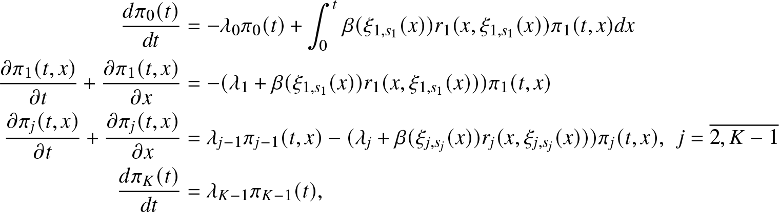 \begin{align*}
\frac{d \pi_0 (t)}{dt}& = - \lambda_0 \pi_0(t) + \int_0^t \beta (\xi_{1,s_1}(x)) r_1(x, \xi_{1,s_1}(x)) \pi_1(t,x) dx \\
\frac{\partial \pi_1 (t,x)}{\partial t} + \frac{\partial \pi_1 (t,x)}{\partial x} &= - (\lambda_1 + \beta(\xi_{1,s_1}(x)) r_1(x, \xi_{1,s_1}(x))) \pi_1(t,x)\\
\frac{\partial \pi_j (t,x)}{\partial t} + \frac{\partial \pi_j (t,x)}{\partial x} &= \lambda_{j-1} \pi_{j-1}(t,x)- (\lambda_j + \beta(\xi_{j,s_j}(x)) r_j(x, \xi_{j,s_j}(x))) \pi_j(t,x),\,\,\, j= \overline{2,K-1}\\
\frac{d \pi_K(t)}{dt} &= \lambda_{K-1} \pi_{K-1}(t),
\end{align*}
\begin{align*}
\frac{d \pi_0 (t)}{dt}& = - \lambda_0 \pi_0(t) + \int_0^t \beta (\xi_{1,s_1}(x)) r_1(x, \xi_{1,s_1}(x)) \pi_1(t,x) dx \\
\frac{\partial \pi_1 (t,x)}{\partial t} + \frac{\partial \pi_1 (t,x)}{\partial x} &= - (\lambda_1 + \beta(\xi_{1,s_1}(x)) r_1(x, \xi_{1,s_1}(x))) \pi_1(t,x)\\
\frac{\partial \pi_j (t,x)}{\partial t} + \frac{\partial \pi_j (t,x)}{\partial x} &= \lambda_{j-1} \pi_{j-1}(t,x)- (\lambda_j + \beta(\xi_{j,s_j}(x)) r_j(x, \xi_{j,s_j}(x))) \pi_j(t,x),\,\,\, j= \overline{2,K-1}\\
\frac{d \pi_K(t)}{dt} &= \lambda_{K-1} \pi_{K-1}(t),
\end{align*} with initial condition  $\pi_0(0)=1$ and boundary conditions
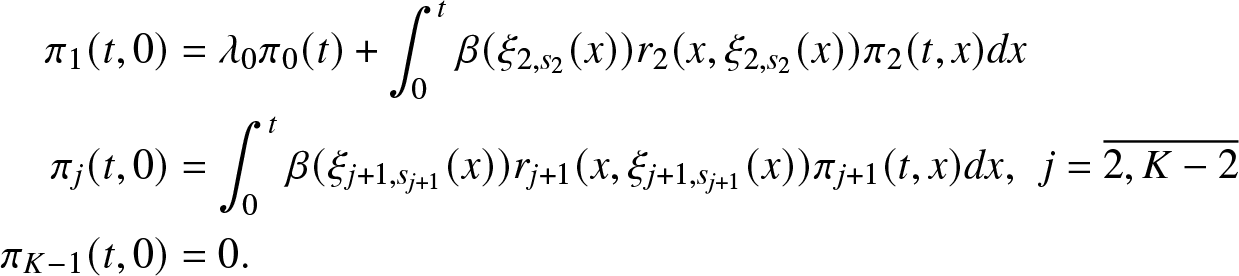 \begin{align*}
\pi_1(t,0) &= \lambda_0 \pi_0(t) + \int_0^t \beta (\xi_{2,s_2}(x)) r_2 (x, \xi_{2,s_2}(x)) \pi_2(t,x) dx \\
\pi_j(t,0) &= \int_0^t \beta (\xi_{j+1,s_{j+1}}(x)) r_{j+1} (x, \xi_{j+1,s_{j+1}}(x)) \pi_{j+1}(t,x) dx, \,\,\,j= \overline{2,K-2} \\
\pi_{K-1}(t,0) &= 0.
\end{align*}
\begin{align*}
\pi_1(t,0) &= \lambda_0 \pi_0(t) + \int_0^t \beta (\xi_{2,s_2}(x)) r_2 (x, \xi_{2,s_2}(x)) \pi_2(t,x) dx \\
\pi_j(t,0) &= \int_0^t \beta (\xi_{j+1,s_{j+1}}(x)) r_{j+1} (x, \xi_{j+1,s_{j+1}}(x)) \pi_{j+1}(t,x) dx, \,\,\,j= \overline{2,K-2} \\
\pi_{K-1}(t,0) &= 0.
\end{align*}Proof. See Appendix A.2.
The statement of Theorem 3.2 implies that the variations of micro-state PDF and of macro-probabilities over infinitesimal intervals obey a set of PDEs with initial and boundary conditions.
The equations of the PDE system have a flow-of-probability interpretation form. When we consider, as an example, the state i and the repair time x, the net rate of flow of probability into this state (i, x) is  $\frac{\partial \pi_{i}(t,x)}{\partial t}+\frac{\partial \pi_{i}(t,x)}{\partial x}$. It is composed of: the inward flow rate, which consists of the density $\pi_{i-1}(t,x)$ multiplied by the rate $\lambda_{i-1}$ at which a failure occurs, having the overall system already i − 1 failed components; the outward flow rate, which is the amount there $\pi_{i}(t,x)$ multiplied by the rate at which transition leaves state (i, x). The leaving of state (i, x) is the summation of the failure mechanism rate (λj) and the repair mechanism ( $\beta(\xi_{j,s_{j}}(x))$); the latter depends on the solution $\xi_{j,s_{j}}(x))$ of the nonlinear ODE defining the modulated repair mechanism and the base repair mechanism of rate $\beta(\cdot)$.
A similar explanation can be given for all the equations, as the net rate of flow of probability is obtained by balancing outward and inward flow rates.
Remark 3.3. It is worth noticing that the system of PDE in Theorem 3.2 has some important differences compared to the result in [Reference Rykov, Kozyrev, Filimonov and Ivanova31]. In fact, first, in all the equations that compose the system, the modulated repair mechanism produces a nonlinear transformation on the function of interest. Second, the modulation makes the (nonlinear) repair rates dependent on the specific state (number of fault components) of the system. This allows a more flexible and general dynamic evolution of the system and could be more representative of real systems. Furthermore, to the best of the authors’ knowledge, this is the first example of a class of models, within the study of the reliability of K-out-of-N system, that describes a nonlinear effort rate function. Clearly, the results in [Reference Rykov, Kozyrev, Filimonov and Ivanova31] are recovered in the very special case described in Eq. (9).
Remark 3.4. In the particular case studied in [Reference Rykov, Kozyrev, Filimonov and Ivanova31], the authors proposed an algorithm for the solution of the system of PDEs that is based on the method of characteristics. In our case, the problem cannot be solved in its generality, as the nonlinear ODE of the modulated repair rate mechanism in general cannot be solved analytically. Thus, the solution needs a case-by-case investigation. A possible alternative is to develop a specific numerical algorithm based on numerical methods such as the finite difference method or finite element method [Reference Larsson and Thomée21]. This problem deserves a specific and dedicated study.
3.3. Ordering of reliability functions
Let us now consider the problem of comparing the reliability functions of two systems of the type considered before. We will denote by  $J^{(i)}(t)$ and $J^{(j)}(t)$ the number of fault components at time t of system (i) and of system (j), respectively. We are interested in obtaining sufficient conditions so that the reliability of one system is greater than the reliability of the other system uniformly over time. One possibility is to work directly on the system of PDEs describing the evolution of the macro- and micro-state probabilities and try to resort to monotonicity conditions about its solution. This approach can be inaccessible because of the inherent difficulties in getting analytical solutions of the Kolmogorov forward system of PDE.
The alternative idea is to construct a third K-out-of-N system that is proved to be between processes  $J^{(i)}(t)$ and $J^{(j)}(t)$ and for which comparison with both original systems is much easier.
To develop this strategy, some auxiliary concepts are needed from the stochastic ordering of random variables (see, e.g., [Reference Gupta14, Reference Kijima and Ohnishi17]).
Definition 3.5. Let X and Y be two random variables and denote by FX and FY their CDFs. It is said that X is greater than Y according to the first-order stochastic dominance criterion, that is,  $X\geq _{FSD} Y$, if $F_{X}(t)\leq F_{Y}(t)$, $\forall t$.
Definition 3.6. Let X be a nonnegative random variable with CDF FX and density fX. X is increasing hazard rate if  $h_{X}(x) := \frac{f_{X}(x)}{1- F_{X}(x)}$ is an increasing function.
Definition 3.7. Let X and Y be two random variables and denote by  $h_{X}(\cdot)$ and $h_{Y}(\cdot)$ their hazard rate functions. X is greater than Y according to the hazard rate order, that is, $X\geq _{hr} Y$, if $h_{X}(t)\leq h_{Y}(t)$, $\forall t$.
As well known, given two distributions FX and FY, if FX is smaller than FY in the hazard rate order, then FX first-order stochastically dominates FY. That is, if:
 \begin{equation*} h_{X}(t) \leq h_{Y}(t) \quad \text{for all} \; t \geq 0 \Longrightarrow
F_{X}(t) \leq F_{Y}(t) .\end{equation*}
\begin{equation*} h_{X}(t) \leq h_{Y}(t) \quad \text{for all} \; t \geq 0 \Longrightarrow
F_{X}(t) \leq F_{Y}(t) .\end{equation*}The next result is key to providing the ordering of reliability functions.
Theorem 3.8. Let’s assume that for systems (i) and (j), satisfying Assumption F1 and Assumptions R1–R5, further ordering assumptions hold true. Specifically,
• Assumption O1: $r_{h}^{(i)} (x,y) \geq r_{h}^{(j)} (x,y),~ \forall h = 1,\ldots,K-1, \forall x,y \in \mathbb{R}$;
• Assumption O2:
$s_h^{(i)} \geq s_h^{(j)},~ \forall h = 1,\ldots,K-1$;• Assumption O3: The CDF’s
$B^{(i)}(\cdot)$ and
$B^{(j)}(\cdot)$ of the base repair mechanism are increasing hazard rates.


Then,  $R^{(i)}(t) \geq R^{(j)}(t), \forall t \in \mathbb{R_{+}}$.
Proof. See Appendix A.3.
The practical relevance of Theorem 3.8 is that it provides sufficient conditions that determine the external monotonicity of the reliability functions for two K-out-of-N systems of the type considered in Section 2. Specifically, we consider Assumptions O1–O2 involving the Cauchy problem (4) and Assumption O3 on the base repair mechanism so that the reliability function of one system ( $J^{(i)}$) is greater than the reliability function of the other system ( $J^{(j)}$) for any time $t\geq 0$. Given an original system and using pairwise comparisons, we can easily design systems with higher or lower reliability than the original one. Therefore, Theorem 3.8 offers fundamental information that can be used to achieve high reliability and allow an engineer to understand the properties of the system and provide an optimal solution to control the level of risk in time and obtain reliable usage.
4. Numerical illustration
To demonstrate the application of the considered model in practice, an example is designed based on a 2-out-of-3 system. Thus, the system has a complete failure the first time two of the three components fail. It is important to notice that even if the 2-out-of-3 system consists of a low number of components, it is already applied to real problems. A notable example is that of centrifugal water pumps. They are used in main water pipelines to compensate for the drop in water pressure. Their failure results in water outages/shortages in the water supply network, which, in turn, can lead to significant inefficiency and economic losses. To control these risks, it is common practice to design a system with three pumps in parallel, and if two of them are out of service, the water pressure will drop, causing the failure of the water supply network. An in-depth study of this kind of system and its practical relevance can be found in [Reference Mortazavi, Mohamadi and Jouzdani25] and the reference therein.
Here, it is assumed that the failures arrive according to a Poisson process with intensity  $\alpha=1/3$. Therefore, the time-varying system’s failure intensity is
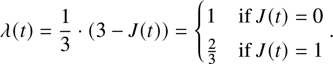 \begin{equation}
\lambda(t)=\frac{1}{3}\cdot (3-J(t))
=\begin{cases}
1 & \text {if } J(t)=0 \\
\frac{2}{3} & \text {if } J(t)=1 \\
\end{cases}.
\end{equation}
\begin{equation}
\lambda(t)=\frac{1}{3}\cdot (3-J(t))
=\begin{cases}
1 & \text {if } J(t)=0 \\
\frac{2}{3} & \text {if } J(t)=1 \\
\end{cases}.
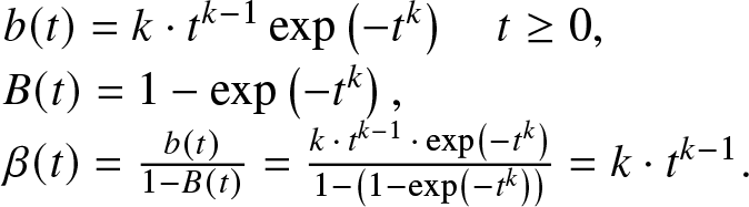
\end{equation} A base repair mechanism described by a Weibull distribution of shape parameter  $k \in (0,+\infty)$ and unitary scale parameter, that is, λ = 1 is considered. Its PDF, CDF, and repair rate functions are as follows:
 \begin{equation*}
\begin{array}{l}
b(t)=k \cdot t^{k-1} \exp \left(-t^k\right) \quad t \geq 0, \\
B(t)=1-\exp \left(-t^k\right), \\
\beta(t)=\frac{b(t)}{1-B(t)}=\frac{k\,\cdot\,t^{k-1}\,\cdot\,\exp \left(-t^k\right)}{1-\left(1-\exp \left(-t^k\right)\right)}=k \cdot t^{k-1}. \\
\end{array}
\end{equation*}
\begin{equation*}
\begin{array}{l}
b(t)=k \cdot t^{k-1} \exp \left(-t^k\right) \quad t \geq 0, \\
B(t)=1-\exp \left(-t^k\right), \\
\beta(t)=\frac{b(t)}{1-B(t)}=\frac{k\,\cdot\,t^{k-1}\,\cdot\,\exp \left(-t^k\right)}{1-\left(1-\exp \left(-t^k\right)\right)}=k \cdot t^{k-1}. \\
\end{array}
\end{equation*}For k > 1, the repair (hazard) rate is increasing in time, and the base repair distribution satisfies the increasing repair rate hypothesis in Theorem 3.8.
Additionally, we need to specify the modulated repair mechanism. The only time periods in which the repair facility is working are during any random interval in which  $J(t)=1$. In fact, when $J(t)=0$ there is no component to repair, while as soon as the system is in the state $J(t)=2$ it stops being in complete failure. Hence, for every time $t\in [T_{i}(\omega),T_{i+1}(\omega))$, the next Cauchy initial value problem is considered to describe the evolution of the effort rate process:
 \begin{equation*}\begin{cases}
\frac{dS(t)}{dt} = 1 + 2 r t\\
S(0) = 0
\end{cases}\!\!\!\!\!.\end{equation*}
\begin{equation*}\begin{cases}
\frac{dS(t)}{dt} = 1 + 2 r t\\
S(0) = 0
\end{cases}\!\!\!\!\!.\end{equation*} The solution of the Cauchy problem is  $S(t) = t + r t^2$. Then, the effort produced to repair the fault components increases in the time elapsed in the repair condition and increases with respect to the parameter r. The hazard (repair) rate function $\beta_1(x) = k(x + r x^2) (1 + 2rx)$ is considered. To solve this example, a specific value for the shape parameter K is set, for example k = 2, so that
 \begin{equation*}
\beta_1 (x) = 2 (x + r x^2) (1 + 2rx)= 2x [1 + 3rx + 2r^2 x^2].
\end{equation*}
\begin{equation*}
\beta_1 (x) = 2 (x + r x^2) (1 + 2rx)= 2x [1 + 3rx + 2r^2 x^2].
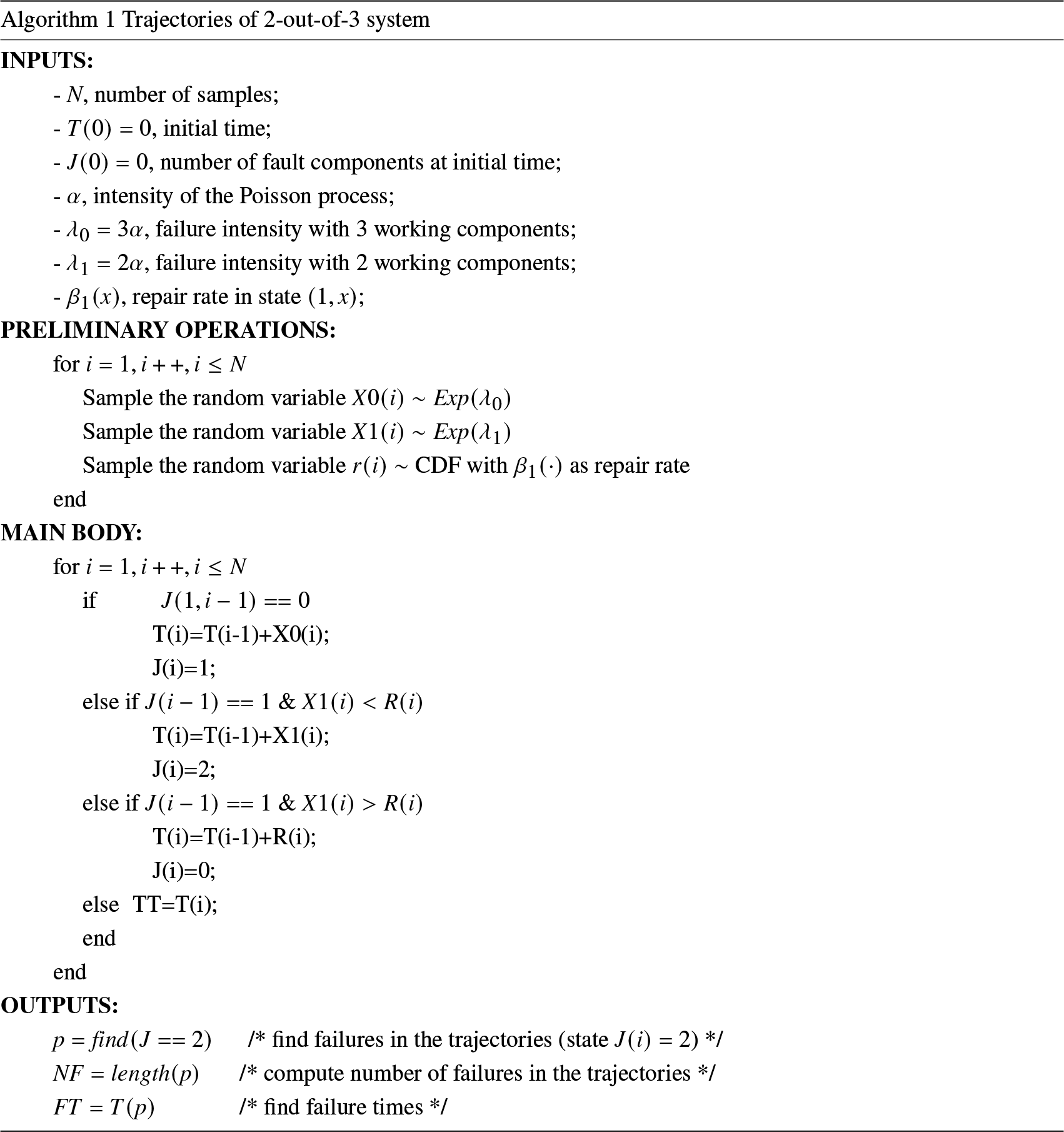
\end{equation*} A Monte Carlo method can be applied to estimate the reliability function. The technique is easily adaptable to handle multicomponent systems and represents a viable alternative to analytical solutions of the PDE system, which is possible only for simplified forms of the model considered. The algorithm is made up of four parts. In the first one, the inputs of the model are listed. It is important to note that the repair rate  $\beta_{1}(x)$ should be calculated using the relation (8), which uses the base repair rate $\beta(x)$ and the solution of the ODE defining the effort function process. The second part considers some preliminary operations that are executed outside of the main body of the algorithm for the sake of clarity. Here, failure times are simulated when there are only working components ( $X0(\cdot)$) and when there is one faulty component ( $X1(\cdot)$). Furthermore, the simulation of the repair times (r(i)) is also executed according to the repair rate $\beta_{1}(x)$.
The main body of the algorithm is devoted to the simulation of concatenated sequences of states (J(i)) and transition times (T(i)). This part is easily scalable to systems with more components. The final part concerns the outputs of the algorithm. They consist of finding the failures in the trajectories, computing the corresponding number of failures, and the failure times. Finally, the reliability function can be estimated by using standard nonparametric techniques applied to lifetime data.
The problem is solved for different values r to show the increasing of the monotonicity property of the reliability function discussed in Theorem 3.8.
In Figure 1, the reliability function corresponding to the value of r = 1 is displayed. The continuous line shows the reliability evaluated by Monte Carlo simulation and includes the confidence interval at the significance level of 95%.
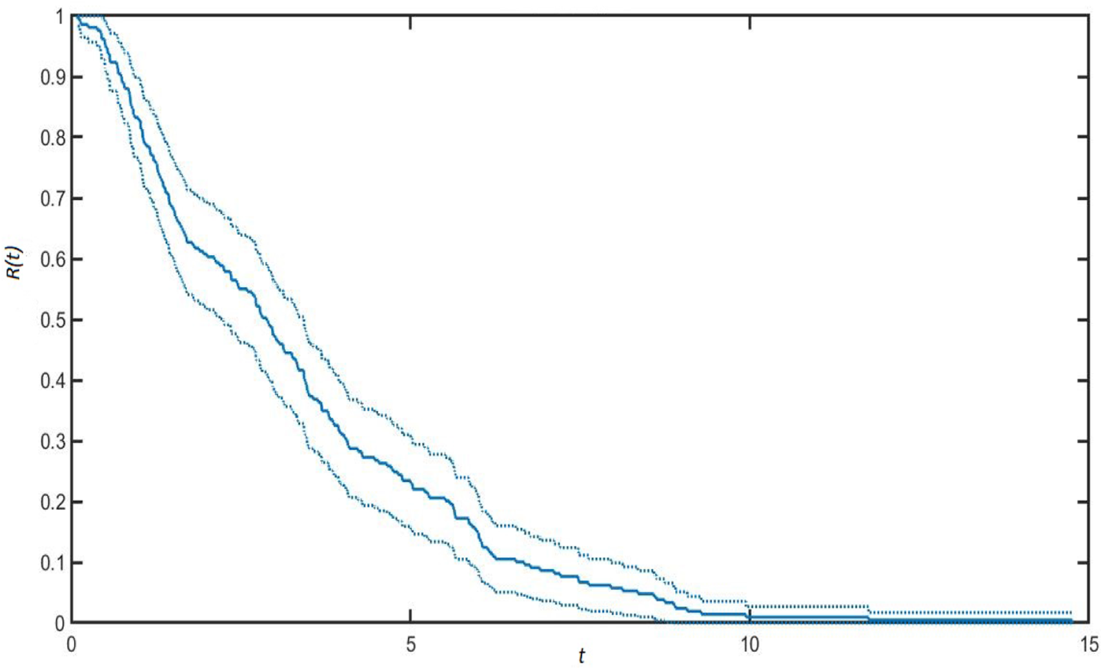
Figure 1. Reliability function for parameter r = 1 and 95% confidence interval.
In Figure 2, the reliability function corresponding to the value of r = 4 is displayed, and in Figure 3 the case for r = 15 is shown.
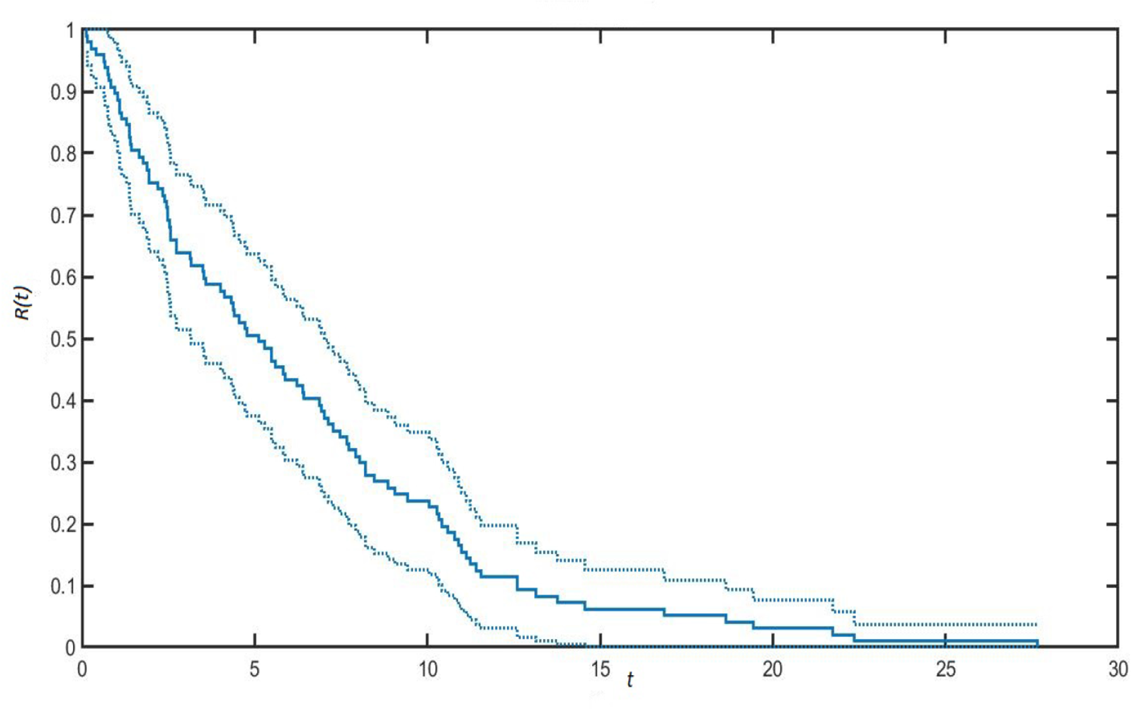
Figure 2. Reliability function for parameter r = 4 and 95% confidence interval.
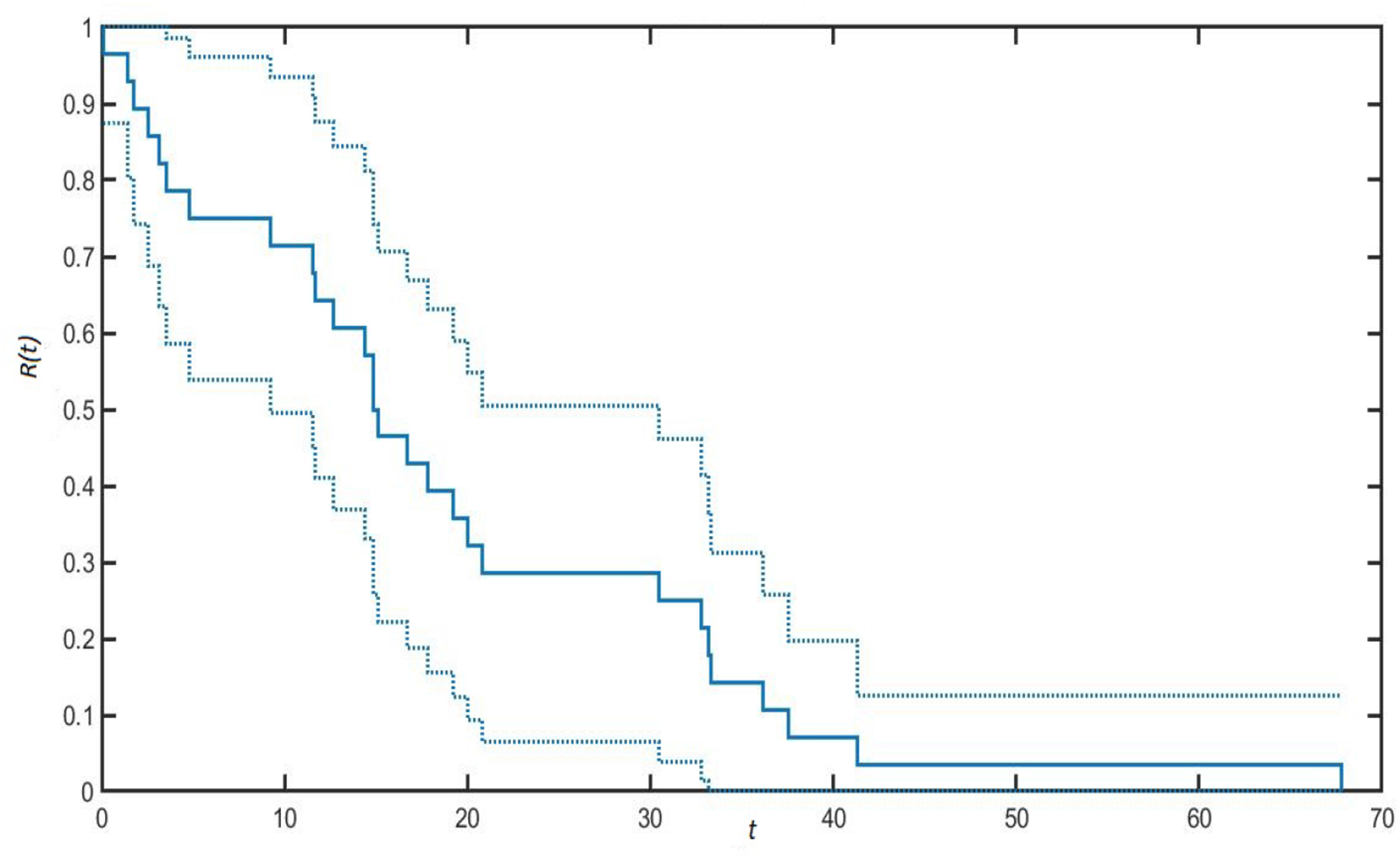
Figure 3. Reliability function for parameter r = 15 and 95% confidence interval.
A direct comparison reveals that the reliability function assumes greater values as the parameter r increases. This means that if effort in repairing the fault component increases, the system’s lifetime is increased, and hence the reliability function. It is observed that the reliability function has a smoother curve for small values of r and this is accompanied by narrow confidence bands. The reason for this can be found in having fixed the same number of total simulations in the experiments. Whenever r is low, repairs are less probable, and the system experiences more default events, which produces a smoother reliability function and narrow confidence intervals. The opposite happens for large values of r.
A final comparison is made with respect to the repair mechanism considered in [Reference Rykov, Kozyrev, Filimonov and Ivanova31], which is the recovered setting r = 0 in our numerical example. In this case, the results are summarized in Figure 4. As expected, the reliability function is lower as the modulated repair mechanism does not allow for an increasing effort to improve the system performance. Summarizing, numerical results show that the inclusion of a random effort function is particularly beneficial as it affects the reliability of the system. In this framework, the reliability engineer can modulate the repair action with the objective of increasing the system’s reliability.
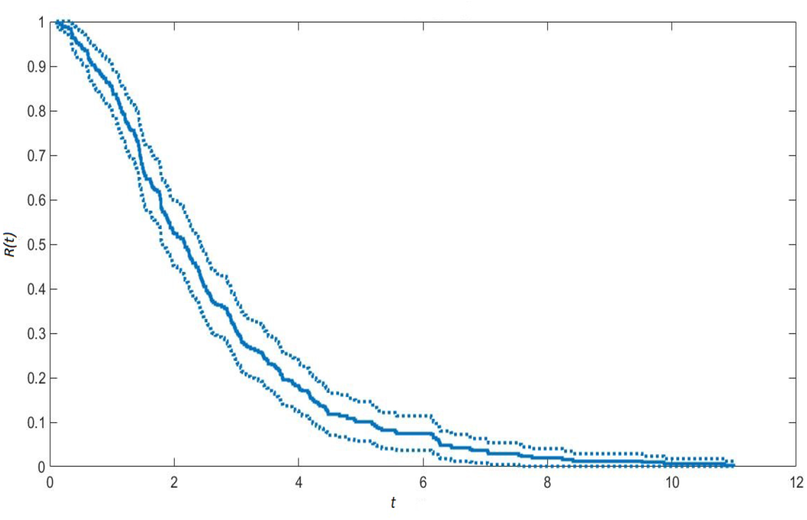
Figure 4. Reliability function for parameter r = 0 and 95% confidence interval.
5. Conclusions and future directions
In this study, a repairable K-out-of-N system with a new repair mechanism is proposed. It considers a random effort function, which is described by a nonlinear ordinary differential equation that modulates the base repair mechanism. Therefore, the system designs a very flexible repair mechanism that generalizes previous contributions in the field. The more general framework needs a rigorous mathematical investigation that leads to a number of results, including regularity properties of the system, Kolmogorov forward PDE for microstate densities, and ordering relations for the reliability function. A numerical example confirms the theoretical results for a 2-out-of-3 system. It demonstrates the possible application of the proposed model to real problems. A Monte Carlo algorithm is implemented to calculate the reliability functions for different parameters. The ordering relation among these functions is visualized as a confirmation of the theory.
The future works for the underlying study include:
• the solution of the system of PDE by means of specific numerical methods;
• the computation of other performability metrics;
• the implementation of real applications to system requiring installed resources with limited capacity.
Acknowledgments
G. D’Amico acknowledges financial support from the European Union—NextGenerationEU. Project PRIN 2022 “Stochastic models and techniques for the management of wind farms and power systems” code: 2022ETEHRM CUP D53D23006470006.
G. D’Amico is a member of the Gruppo Nazionale Calcolo Scientifico-Istituto Nazionale di Alta Matematica (GNCS-INdAM).
Dharmaraja Selvamuthu thanks the financial support of DST-RSF research project no. 22-49-02023 (RSF) and research project no. 64800 (DST).
We also thank the anonymous referees for their helpful comments and suggestions.
Competing interest
The authors declare that they have no known competing financial interests or personal relationships that could have appeared to influence the work reported in this paper.
Appendix
A.1. Proof of Lemma 3.1
Proof. For notation convenience, the information set  $\{J(t) = i, X(t)=x, S(t)= \xi_{i,s_{i}}(x)\}$ is denoted in compact form as $(i,x,\xi)$ where no ambiguity may arise. Let us also introduce the notation $\Delta N(t):=N(t+\Delta t)-N(t)$ as the increment of the counting process over the time interval $(t, t+\Delta t)$.
Let us consider the probability:
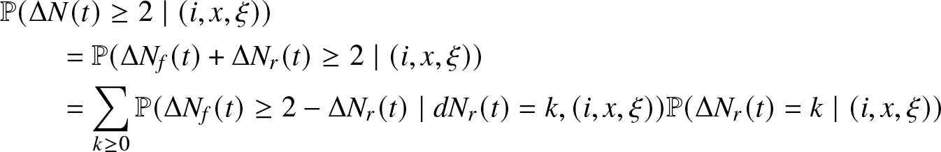 \begin{align*}
&\mathbb{P} (\Delta N(t) \geq 2 \mid (i,x, \xi))\\
& \qquad = \mathbb{P} (\Delta N_f(t) + \Delta N_r (t) \geq 2 \mid (i,x, \xi))\\
&\qquad = \sum_{k \geq 0} \mathbb{P} (\Delta N_f(t) \geq 2 - \Delta N_r (t) \mid d N_r (t) =k, (i,x, \xi)) \mathbb{P} (\Delta N_r(t)=k \mid (i,x, \xi))
\end{align*}
\begin{align*}
&\mathbb{P} (\Delta N(t) \geq 2 \mid (i,x, \xi))\\
& \qquad = \mathbb{P} (\Delta N_f(t) + \Delta N_r (t) \geq 2 \mid (i,x, \xi))\\
&\qquad = \sum_{k \geq 0} \mathbb{P} (\Delta N_f(t) \geq 2 - \Delta N_r (t) \mid d N_r (t) =k, (i,x, \xi)) \mathbb{P} (\Delta N_r(t)=k \mid (i,x, \xi))
\end{align*} \begin{equation}
\!\!\!\!\!\!\!\!\!\!\!\!\!\!\!\!\!\!= \mathbb{P} (\Delta N_f(t) \geq 2 \mid d N_r (t) =0, (i,x, \xi)) \mathbb{P} (\Delta N_r(t)=0 \mid (i,x, \xi))
\end{equation}
\begin{equation}
\!\!\!\!\!\!\!\!\!\!\!\!\!\!\!\!\!\!= \mathbb{P} (\Delta N_f(t) \geq 2 \mid d N_r (t) =0, (i,x, \xi)) \mathbb{P} (\Delta N_r(t)=0 \mid (i,x, \xi))
\end{equation} \begin{equation}
\!\!\!\!\!\!\!\!\!+\,\mathbb{P} (\Delta N_f(t) \geq 1 \mid d N_r (t) =1, (i,x, \xi)) \mathbb{P} (\Delta N_r(t)=1 \mid (i,x, \xi))
\end{equation}
\begin{equation}
\!\!\!\!\!\!\!\!\!+\,\mathbb{P} (\Delta N_f(t) \geq 1 \mid d N_r (t) =1, (i,x, \xi)) \mathbb{P} (\Delta N_r(t)=1 \mid (i,x, \xi))
\end{equation} \begin{equation}
\,\,+\sum_{k \geq 2} \mathbb{P} (\Delta N_f(t) \geq 0 \mid d N_r (t) =k, (i,x, \xi)) \mathbb{P} (\Delta N_r(t)=k \mid (i,x, \xi)).
\end{equation}
\begin{equation}
\,\,+\sum_{k \geq 2} \mathbb{P} (\Delta N_f(t) \geq 0 \mid d N_r (t) =k, (i,x, \xi)) \mathbb{P} (\Delta N_r(t)=k \mid (i,x, \xi)).
\end{equation} Clearly, it is sufficient to show that each one of the previous addenda is an  $o(\Delta t)$.
Let us consider before Eq. (A.3). It is found that
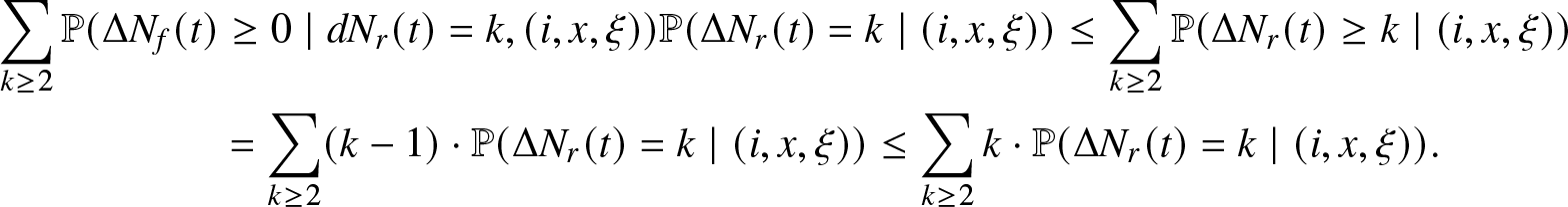 \begin{align*}
\sum_{k \geq 2} \mathbb{P} (\Delta N_f(t) &\geq 0 \mid d N_r (t) =k, (i,x, \xi)) \mathbb{P} (\Delta N_r(t)=k \mid (i,x, \xi)) \leq \sum_{k \geq 2} \mathbb{P} (\Delta N_r(t) \geq k \mid (i,x, \xi))\\
&= \sum_{k \geq 2} (k-1) \cdot \mathbb{P} (\Delta N_r(t) =k \mid (i,x, \xi)) \leq \sum_{k \geq 2} k \cdot \mathbb{P} (\Delta N_r(t) = k \mid (i,x, \xi)).
\end{align*}
\begin{align*}
\sum_{k \geq 2} \mathbb{P} (\Delta N_f(t) &\geq 0 \mid d N_r (t) =k, (i,x, \xi)) \mathbb{P} (\Delta N_r(t)=k \mid (i,x, \xi)) \leq \sum_{k \geq 2} \mathbb{P} (\Delta N_r(t) \geq k \mid (i,x, \xi))\\
&= \sum_{k \geq 2} (k-1) \cdot \mathbb{P} (\Delta N_r(t) =k \mid (i,x, \xi)) \leq \sum_{k \geq 2} k \cdot \mathbb{P} (\Delta N_r(t) = k \mid (i,x, \xi)).
\end{align*} Now, consider the probability  $\mathbb{P} (\Delta N_r(t) = k \mid (i,x, \xi))$. Note that the random variable Tn is the arrival time of the nth repair of the counting process $N_{r}(t)$. Hence, we have the relationship that the number of repairs in $(t, t+\Delta t)$ is k if and only if the kth renewal occurs in $(t,t+\Delta t)$ and the (k+1)th renewal occurs after $t+\Delta t$. Formally,
 \begin{equation}
\Delta N_{r}(t)=k \iff \{T_{N(t)+k}\in (t,t+\Delta t), T_{N(t)+k+1} \gt t+\Delta t\}.
\end{equation}
\begin{equation}
\Delta N_{r}(t)=k \iff \{T_{N(t)+k}\in (t,t+\Delta t), T_{N(t)+k+1} \gt t+\Delta t\}.
\end{equation}From (A.4), we obtain
 \begin{equation*}
\mathbb{P} (\Delta N_r(t) = k \mid (i,x, \xi)) = \mathbb{P} (T_{N(t)+k}\in (t,t+\Delta t), T_{N(t)+k+1} \gt t+\Delta t) \leq
\mathbb{P} (T_{N(t)+k}-t \leq \Delta t \mid (i,x, \xi)).
\end{equation*}
\begin{equation*}
\mathbb{P} (\Delta N_r(t) = k \mid (i,x, \xi)) = \mathbb{P} (T_{N(t)+k}\in (t,t+\Delta t), T_{N(t)+k+1} \gt t+\Delta t) \leq
\mathbb{P} (T_{N(t)+k}-t \leq \Delta t \mid (i,x, \xi)).
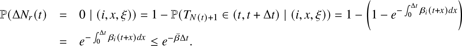
\end{equation*}Consider before the case when k = 1.
 \begin{equation}
\mathbb{P} (T_{N(t)+1}-t \leq \Delta t \mid (i,x, \xi)) = 1 - e^{- \int_{0}^{\Delta t} \beta_{i} (t+x) dx},
\end{equation}
\begin{equation}
\mathbb{P} (T_{N(t)+1}-t \leq \Delta t \mid (i,x, \xi)) = 1 - e^{- \int_{0}^{\Delta t} \beta_{i} (t+x) dx},
\end{equation} where according to Assumption R5  $\beta_{i} (t+x) = \beta (\xi_{i,s_{i}}(x)) r_i (x, \xi_{i,s_{i}}(x)).$
From Assumption R3, the solution  $\xi_{i,s_{i}}(x)$ is bounded $\forall x \in (0, \Delta t]$ and according to Assumption R2 there exists a real number $\bar{\beta}_{\Delta t} \in \mathbb{R}$ such that
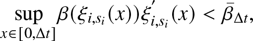 \begin{equation*}
\displaystyle \underset{x \in [0, \Delta t]}{\sup} \beta (\xi_{i,s_{i}}(x)) \xi_{i,s_{i}}^{'}(x) \lt \bar{\beta}_{\Delta t},
\end{equation*}
\begin{equation*}
\displaystyle \underset{x \in [0, \Delta t]}{\sup} \beta (\xi_{i,s_{i}}(x)) \xi_{i,s_{i}}^{'}(x) \lt \bar{\beta}_{\Delta t},
\end{equation*} because the composition of two bounded functions is bounded and from the global uniform Lipschitz continuity of the rate of effort function (Assumption R4), it can be written, thanks to the Picard–Lindelöf theorem that the solution is also continuously differentiable, hence  $\xi_{i,s_{i}}^{'}(x) \lt \infty$. Hereinafter, $\bar{\beta}_{\Delta t}$ will be denoted simply by $\bar{\beta}$ keeping in mind the dependence on the time interval length $\Delta t$.
Thus, probability (A.5) can be bounded as follow,
 \begin{equation*}
\mathbb{P} (T_{N(t)+1}-t \leq \Delta t \mid (i,x, \xi)) = 1 - e^{- \int_{0}^{\Delta t} \beta_{i} (t+x) dx} \leq 1- e^{- \bar{\beta} \Delta t} \leq \bar{\beta} \Delta t,
\end{equation*}
\begin{equation*}
\mathbb{P} (T_{N(t)+1}-t \leq \Delta t \mid (i,x, \xi)) = 1 - e^{- \int_{0}^{\Delta t} \beta_{i} (t+x) dx} \leq 1- e^{- \bar{\beta} \Delta t} \leq \bar{\beta} \Delta t,
\end{equation*} where the last inequality is true in virtue of the relation  $1- e^{-x} \leq x, \forall x \geq 0$.
Using previous obtained inequality and the expression of  $ \mathbb{P} (T_{N(t)+k}-t \leq \Delta t \mid (i,x, \xi))$, the following computation is carried out.
Assume that  $ \mathbb{P} (T_{N(t)+k-1}-t \leq \Delta t \mid (i,x, \xi)) \leq (\bar{\beta} \Delta t)^{k-1}$ holds true. It can be obtained that
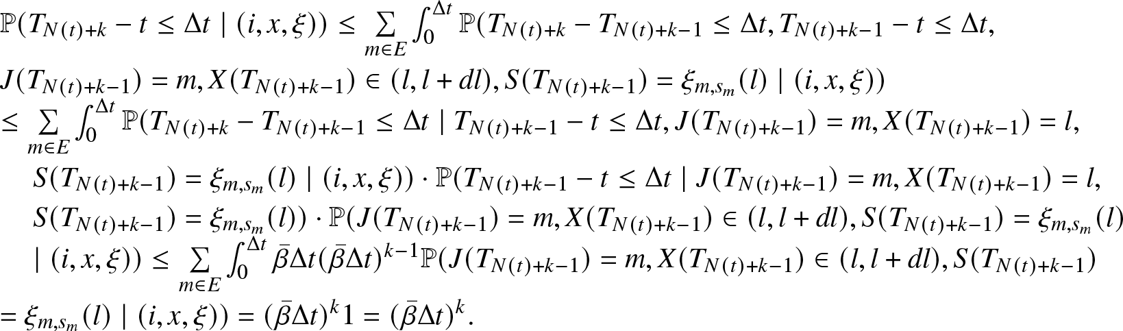 \begin{equation*}\begin{array}{l}
\mathbb{P} (T_{N(t)+k}-t \leq \Delta t \mid (i,x, \xi)) \leq \sum\limits_{m \in E} \int_{0}^{\Delta t} \mathbb{P}(T_{N(t)+k} - T_{N(t)+k-1} \leq \Delta t, T_{N(t)+k-1}-t \leq \Delta t, \\
J(T_{N(t)+k-1})= m, X(T_{N(t)+k-1}) \in (l, l + dl), S(T_{N(t)+k-1}) = \xi_{m, s_{m} } (l) \mid (i,x, \xi))\\
\leq \sum\limits\limits_{m \in E} \int_{0}^{\Delta t} \mathbb{P}(T_{N(t)+k} - T_{N(t)+k-1} \leq \Delta t \mid T_{N(t)+k-1} - t \leq \Delta t, J(T_{N(t)+k-1})= m, X(T_{N(t)+k-1})=l,\\
\,\,\,\,\,\,\,S(T_{N(t)+k-1}) = \xi_{m, s_{m}} (l) \mid (i,x, \xi)) \cdot \mathbb{P}(T_{N(t)+k-1} - t \leq \Delta t \mid J (T_{N(t)+k-1}) = m, X(T_{N(t)+k-1})= l, \\
\,\,\,\,\,\,\,S(T_{N(t)+k-1}) = \xi_{m, s_{m}} (l) ) \cdot \mathbb{P}(J (T_{N(t)+k-1}) = m, X(T_{N(t)+k-1}) \in (l, l + dl), S(T_{N(t)+k-1}) = \xi_{m, s_{m}} (l) \\
\,\,\,\,\,\,\,\mid (i,x, \xi)) \leq \sum\limits_{m \in E} \int_{0}^{\Delta t} \bar{\beta} \Delta t (\bar{\beta} \Delta t)^{k-1} \mathbb{P}(J(T_{N(t)+k-1})=m, X(T_{N(t)+k-1}) \in (l, l+dl),S(T_{N(t)+k-1}) \\
= \xi_{m, s_{m}} (l) \mid (i,x, \xi)) =(\bar{\beta}\Delta t)^{k} {1} = (\bar{\beta} \Delta t)^{k}.
\end{array}\end{equation*}
\begin{equation*}\begin{array}{l}
\mathbb{P} (T_{N(t)+k}-t \leq \Delta t \mid (i,x, \xi)) \leq \sum\limits_{m \in E} \int_{0}^{\Delta t} \mathbb{P}(T_{N(t)+k} - T_{N(t)+k-1} \leq \Delta t, T_{N(t)+k-1}-t \leq \Delta t, \\
J(T_{N(t)+k-1})= m, X(T_{N(t)+k-1}) \in (l, l + dl), S(T_{N(t)+k-1}) = \xi_{m, s_{m} } (l) \mid (i,x, \xi))\\
\leq \sum\limits\limits_{m \in E} \int_{0}^{\Delta t} \mathbb{P}(T_{N(t)+k} - T_{N(t)+k-1} \leq \Delta t \mid T_{N(t)+k-1} - t \leq \Delta t, J(T_{N(t)+k-1})= m, X(T_{N(t)+k-1})=l,\\
\,\,\,\,\,\,\,S(T_{N(t)+k-1}) = \xi_{m, s_{m}} (l) \mid (i,x, \xi)) \cdot \mathbb{P}(T_{N(t)+k-1} - t \leq \Delta t \mid J (T_{N(t)+k-1}) = m, X(T_{N(t)+k-1})= l, \\
\,\,\,\,\,\,\,S(T_{N(t)+k-1}) = \xi_{m, s_{m}} (l) ) \cdot \mathbb{P}(J (T_{N(t)+k-1}) = m, X(T_{N(t)+k-1}) \in (l, l + dl), S(T_{N(t)+k-1}) = \xi_{m, s_{m}} (l) \\
\,\,\,\,\,\,\,\mid (i,x, \xi)) \leq \sum\limits_{m \in E} \int_{0}^{\Delta t} \bar{\beta} \Delta t (\bar{\beta} \Delta t)^{k-1} \mathbb{P}(J(T_{N(t)+k-1})=m, X(T_{N(t)+k-1}) \in (l, l+dl),S(T_{N(t)+k-1}) \\
= \xi_{m, s_{m}} (l) \mid (i,x, \xi)) =(\bar{\beta}\Delta t)^{k} {1} = (\bar{\beta} \Delta t)^{k}.
\end{array}\end{equation*}The above computation gives us the following estimate;
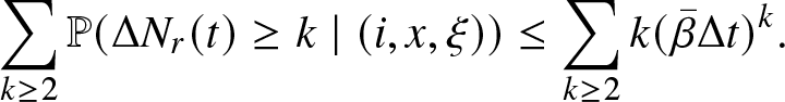 \begin{equation*}
\sum_{k \geq 2} \mathbb{P} (\Delta N_r(t) \geq k \mid (i,x, \xi)) \leq \sum_{k \geq 2} k (\bar{\beta}\Delta t)^{k}.
\end{equation*}
\begin{equation*}
\sum_{k \geq 2} \mathbb{P} (\Delta N_r(t) \geq k \mid (i,x, \xi)) \leq \sum_{k \geq 2} k (\bar{\beta}\Delta t)^{k}.
\end{equation*}This clearly implies that
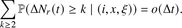 \begin{equation*}
\sum_{k \geq 2} \mathbb{P} (\Delta N_r(t) \geq k \mid (i,x, \xi)) = o(\Delta t).
\end{equation*}
\begin{equation*}
\sum_{k \geq 2} \mathbb{P} (\Delta N_r(t) \geq k \mid (i,x, \xi)) = o(\Delta t).
\end{equation*} Next, consider probability (A.1):  $ \mathbb{P} (\Delta N_f(t) \geq 2 \mid \Delta N_r (t) =0, (i,x, \xi)) \cdot \mathbb{P} (\Delta N_r (t) =0 \mid (i,x, \xi))$. It is observed that
 \begin{equation*}\begin{array}{rcl}
\mathbb{P} (\Delta N_r (t) & =& 0 \mid (i,x, \xi)) = {1} - \mathbb{P} (T_{N(t)+1} \in (t, t+ \Delta t)\mid (i,x, \xi)) =1-\bigg( {1} - e^{- \int_{0}^{\Delta t} \beta_{i} (t+x) dx}\bigg) \\
& =& e^{- \int_{0}^{\Delta t} \beta_{i} (t+x) dx} \leq e^{- \bar{\beta} \Delta t}.
\end{array}\end{equation*}
\begin{equation*}\begin{array}{rcl}
\mathbb{P} (\Delta N_r (t) & =& 0 \mid (i,x, \xi)) = {1} - \mathbb{P} (T_{N(t)+1} \in (t, t+ \Delta t)\mid (i,x, \xi)) =1-\bigg( {1} - e^{- \int_{0}^{\Delta t} \beta_{i} (t+x) dx}\bigg) \\
& =& e^{- \int_{0}^{\Delta t} \beta_{i} (t+x) dx} \leq e^{- \bar{\beta} \Delta t}.
\end{array}\end{equation*} Moreover,  $ \mathbb{P} (\Delta N_f(t) \geq 2 \mid \Delta N_r (t) =0, (i,x, \xi)) = o (\Delta t)$ as the failure occurs according to a Poisson process with intensity $\lambda_i = (n-i) \alpha$, which is finite according to Assumption F1. Hence, probability (A.1) is $o(\Delta t)$.
It remains to compute probability (A.2):
 \begin{equation*}\mathbb{P} (\Delta N_f(t) \geq 1 \mid \Delta N_r (t) =1, (i,x, \xi)) \cdot \mathbb{P} (\Delta N_r (t) =1 \mid (i,x, \xi)).\end{equation*}
It is observed that
 \begin{equation*}
\mathbb{P} (\Delta N_r(t) = 1 \mid (i,x, \xi)) = \mathbb{P} (T_{N_r(t)+1} \in (t, t + \Delta t) \mid (i,x, \xi)) = 1- 1-e^{-\int_0^{\Delta t} \beta_{i} (t+x) dx} \leq \bar{\beta} \Delta t.
\end{equation*}
\begin{equation*}
\mathbb{P} (\Delta N_r(t) = 1 \mid (i,x, \xi)) = \mathbb{P} (T_{N_r(t)+1} \in (t, t + \Delta t) \mid (i,x, \xi)) = 1- 1-e^{-\int_0^{\Delta t} \beta_{i} (t+x) dx} \leq \bar{\beta} \Delta t.
\end{equation*}Next, consider
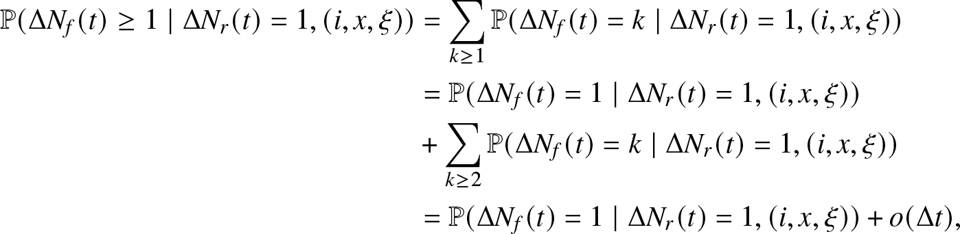 \begin{align*}
\mathbb{P} (\Delta N_f(t) \geq 1 \mid \Delta N_r (t) =1, (i,x, \xi)) &= \sum_{k \geq 1} \mathbb{P} (\Delta N_f(t) = k \mid \Delta N_r (t) =1, (i,x, \xi))\\
&= \mathbb{P} (\Delta N_f(t) = 1 \mid \Delta N_r (t) =1, (i,x, \xi)) \\
&+ \sum\limits_{k \geq 2} \mathbb{P} (\Delta N_f(t) = k \mid \Delta N_r (t) =1, (i,x, \xi))\\
&= \mathbb{P} (\Delta N_f(t) = 1 \mid \Delta N_r (t) =1, (i,x, \xi)) + o (\Delta t),
\end{align*}
\begin{align*}
\mathbb{P} (\Delta N_f(t) \geq 1 \mid \Delta N_r (t) =1, (i,x, \xi)) &= \sum_{k \geq 1} \mathbb{P} (\Delta N_f(t) = k \mid \Delta N_r (t) =1, (i,x, \xi))\\
&= \mathbb{P} (\Delta N_f(t) = 1 \mid \Delta N_r (t) =1, (i,x, \xi)) \\
&+ \sum\limits_{k \geq 2} \mathbb{P} (\Delta N_f(t) = k \mid \Delta N_r (t) =1, (i,x, \xi))\\
&= \mathbb{P} (\Delta N_f(t) = 1 \mid \Delta N_r (t) =1, (i,x, \xi)) + o (\Delta t),
\end{align*}where the last equality follows from the property of the Poisson process governing the failure mechanism.
Since  $\Delta N_r (t) =1, \exists t^* \in (t, t + \Delta t)$ where the component under repair is repaired. This means that in the interval $(t,t^*)$ the $N_f(t)$ process had an intensity $\lambda_i = (n-i) \alpha$ while in the $(t^*, t + \Delta t)$ was $\lambda_{i-1} = (n-i+1) \alpha \geq \lambda_i$. Therefore, it can be bounded
 \begin{align*}
\mathbb{P} (\Delta N_f(t) = 1 \mid \Delta N_r (t) =1, (i,x, \xi)) &\leq \mathbb{P} (\Delta N_f(t) = 1 \mid J(t) =i-1)\\
&= \lambda_{i-1} \Delta t e^{- \lambda_{i-1} \Delta t} \leq \lambda_{i-1} \Delta t.
\end{align*}
\begin{align*}
\mathbb{P} (\Delta N_f(t) = 1 \mid \Delta N_r (t) =1, (i,x, \xi)) &\leq \mathbb{P} (\Delta N_f(t) = 1 \mid J(t) =i-1)\\
&= \lambda_{i-1} \Delta t e^{- \lambda_{i-1} \Delta t} \leq \lambda_{i-1} \Delta t.
\end{align*}Hence, the final result is
 \begin{equation*}\begin{array}{l}
\mathbb{P} (\Delta N_f(t) \geq 1 \mid d N_r (t) =1, (i,x, \xi)) \cdot \mathbb{P} (d N_r (t) =1 \mid (i,x, \xi)) \leq \bar{\beta} \Delta t \lambda_{i-1} \Delta t + o (\Delta t) \\
= \bar{\beta} \lambda_{i-1} (\Delta t)^2 + o (\Delta t) = o (\Delta t). \end{array}\end{equation*}
\begin{equation*}\begin{array}{l}
\mathbb{P} (\Delta N_f(t) \geq 1 \mid d N_r (t) =1, (i,x, \xi)) \cdot \mathbb{P} (d N_r (t) =1 \mid (i,x, \xi)) \leq \bar{\beta} \Delta t \lambda_{i-1} \Delta t + o (\Delta t) \\
= \bar{\beta} \lambda_{i-1} (\Delta t)^2 + o (\Delta t) = o (\Delta t). \end{array}\end{equation*} Thus, it can be concluded that  $\mathbb{P} (\Delta N(t) \geq 2 \mid (i,x, \xi)) = o (\Delta t)$.
A.2. Proof of Theorem 3.2
Proof. The differential equation for the macro-state probability  $\pi_0 (t) = \mathbb{P}(J(t)=0)$ can be proven. Immediately, we have
 \begin{align}
\pi_0 (t + \Delta t) = \mathbb{P}(J(t + \Delta t)=0) = \sum_{l \geq 0} \sum_{i=0}^{K-1} \mathbb{P}(J(t + \Delta t)=0, J(t)=i, \Delta N(t) = l),
\end{align}
\begin{align}
\pi_0 (t + \Delta t) = \mathbb{P}(J(t + \Delta t)=0) = \sum_{l \geq 0} \sum_{i=0}^{K-1} \mathbb{P}(J(t + \Delta t)=0, J(t)=i, \Delta N(t) = l),
\end{align} \begin{align}
\!\!\!\!\!\!\!\!\!\!\!\!\!\!\!\!\!\!\!\!\!\!\!\!\!\!\!\!\!\!\!\!\!\!\!\!\!= \mathbb{P}(J(t + \Delta t)=0, J(t)=0, \Delta N(t) = 0)
\end{align}
\begin{align}
\!\!\!\!\!\!\!\!\!\!\!\!\!\!\!\!\!\!\!\!\!\!\!\!\!\!\!\!\!\!\!\!\!\!\!\!\!= \mathbb{P}(J(t + \Delta t)=0, J(t)=0, \Delta N(t) = 0)
\end{align} \begin{align}
\!\!\!\!\!\!\!+\,\mathbb{P}(J(t + \Delta t)=0, J(t)=1, \Delta N(t) = 1) + o (\Delta t),
\end{align}
\begin{align}
\!\!\!\!\!\!\!+\,\mathbb{P}(J(t + \Delta t)=0, J(t)=1, \Delta N(t) = 1) + o (\Delta t),
\end{align}where the last relation comes from regularity results given in Lemma 3.1. Now consider relation (A.7), and observe that
 \begin{equation*}
\Delta N(t)=0 \iff \Delta_{f}(t)=0\,\,\, \text{and}\,\,\, \Delta_{r}(t)=0.
\end{equation*}
\begin{equation*}
\Delta N(t)=0 \iff \Delta_{f}(t)=0\,\,\, \text{and}\,\,\, \Delta_{r}(t)=0.
\end{equation*}Accordingly we have that
 \begin{align*}
\mathbb{P}(J(t + \Delta t)=0, J(t)=0, \Delta N(t) = 0) &=
\mathbb{P}(\Delta N_{r}(t) = 0, J(t + \Delta t)=0 \mid J(t)=0, \Delta N_{f}(t) = 0)\\
&\quad\cdot\,\mathbb{P}(\Delta N_{f}(t) = 0 \mid J(t)=0) \cdot \mathbb{P}(J(t)=0).
\end{align*}
\begin{align*}
\mathbb{P}(J(t + \Delta t)=0, J(t)=0, \Delta N(t) = 0) &=
\mathbb{P}(\Delta N_{r}(t) = 0, J(t + \Delta t)=0 \mid J(t)=0, \Delta N_{f}(t) = 0)\\
&\quad\cdot\,\mathbb{P}(\Delta N_{f}(t) = 0 \mid J(t)=0) \cdot \mathbb{P}(J(t)=0).
\end{align*} We first observe that  $\mathbb{P}(\Delta N_{r}(t) = 0, J(t + \Delta t)=0 \mid J(t)=0, \Delta N_{f}(t) = 0)=1$ as, being in a state 0 at time t and not having any failure in the time interval $(t,t+\Delta t)$ implies that no repair can be executed as all the components are working and then $J(t+\Delta t)=0$. Therefore, probability (A.7) equals
 \begin{equation*}\begin{array}{l}
= \mathbb{P}( \Delta N_f(t) = 0 \mid J(t)=0) \times \pi_0 (t)= [{1}- \lambda_0 \Delta t + o(\Delta t)] \cdot \pi_0 (t)\\
= \pi_0 (t) - \pi_0(t) \lambda_0 \Delta t + \pi_{0} (t) o (\Delta t).
\end{array}\end{equation*}
\begin{equation*}\begin{array}{l}
= \mathbb{P}( \Delta N_f(t) = 0 \mid J(t)=0) \times \pi_0 (t)= [{1}- \lambda_0 \Delta t + o(\Delta t)] \cdot \pi_0 (t)\\
= \pi_0 (t) - \pi_0(t) \lambda_0 \Delta t + \pi_{0} (t) o (\Delta t).
\end{array}\end{equation*}Now, consider relation (A.8),
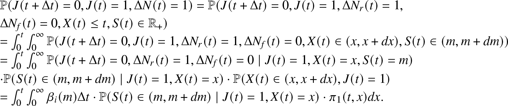 \begin{align}
\begin{array}{l}
\mathbb{P}(J(t + \Delta t)=0, J(t)=1, \Delta N(t) = 1) = \mathbb{P}(J(t + \Delta t)=0, J(t)=1, \Delta N_r(t) = 1,\\
\Delta N_f(t) = 0, X(t) \leq t, S(t) \in \mathbb{R_{+}}) \\
= \int_0^{t} \int_0^{\infty} \mathbb{P}(J(t + \Delta t)=0, J(t)=1, \Delta N_r(t) = 1, \Delta N_f(t) = 0, X(t) \in (x, x + dx), S(t) \in (m, m+dm)) \\
= \int_0^{t} \int_0^{\infty} \mathbb{P}(J(t + \Delta t)=0, \Delta N_r(t) = 1, \Delta N_f(t) = 0 \mid J(t)=1, X(t) =x, S(t)= m) \\
\cdot \mathbb{P}(S(t) \in (m, m+dm) \mid J(t)=1, X(t)=x) \cdot \mathbb{P}(X(t) \in (x, x+dx), J(t)=1) \\
= \int_0^{t} \int_0^{\infty} \beta_i (m) \Delta t \cdot \mathbb{P}(S(t) \in (m, m+dm) \mid J(t)=1, X(t)=x) \cdot \pi_1 (t,x) dx.
\end{array}
\end{align}
\begin{align}
\begin{array}{l}
\mathbb{P}(J(t + \Delta t)=0, J(t)=1, \Delta N(t) = 1) = \mathbb{P}(J(t + \Delta t)=0, J(t)=1, \Delta N_r(t) = 1,\\
\Delta N_f(t) = 0, X(t) \leq t, S(t) \in \mathbb{R_{+}}) \\
= \int_0^{t} \int_0^{\infty} \mathbb{P}(J(t + \Delta t)=0, J(t)=1, \Delta N_r(t) = 1, \Delta N_f(t) = 0, X(t) \in (x, x + dx), S(t) \in (m, m+dm)) \\
= \int_0^{t} \int_0^{\infty} \mathbb{P}(J(t + \Delta t)=0, \Delta N_r(t) = 1, \Delta N_f(t) = 0 \mid J(t)=1, X(t) =x, S(t)= m) \\
\cdot \mathbb{P}(S(t) \in (m, m+dm) \mid J(t)=1, X(t)=x) \cdot \mathbb{P}(X(t) \in (x, x+dx), J(t)=1) \\
= \int_0^{t} \int_0^{\infty} \beta_i (m) \Delta t \cdot \mathbb{P}(S(t) \in (m, m+dm) \mid J(t)=1, X(t)=x) \cdot \pi_1 (t,x) dx.
\end{array}
\end{align} Observe that, S(t) is a random variable that is  $\{J(t), X(t)\}$-measurable. The conditional distribution of S(t) given $J(t)=1, X(t)=x$ is of the Heaviside function $\forall t \in \mathbb{R_{+}}$. Hence,
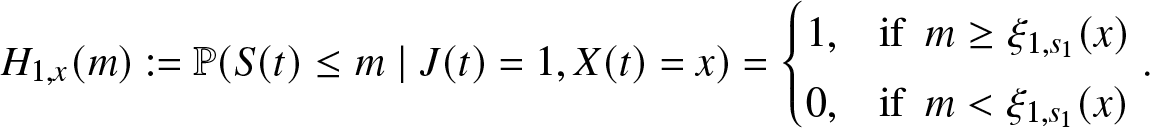 \begin{equation*}H_{1,x}(m):= \mathbb{P}(S(t)\leq m \mid J(t)=1, X(t)=x) = \begin{cases}
1, & \text{if}\,\,\, m \geq \xi_{1, s_1}(x) \\
0, & \text{if}\,\,\, m \lt \xi_{1, s_1}(x)
\end{cases}.\end{equation*}
\begin{equation*}H_{1,x}(m):= \mathbb{P}(S(t)\leq m \mid J(t)=1, X(t)=x) = \begin{cases}
1, & \text{if}\,\,\, m \geq \xi_{1, s_1}(x) \\
0, & \text{if}\,\,\, m \lt \xi_{1, s_1}(x)
\end{cases}.\end{equation*} According to the integral property of a function with respect to a Heaviside distribution (Dirac function)  $\int_{-\infty}^{+ \infty} h (m) dH_{1,x}(m) = h (\xi_{1, s_1}(x))$, then Eq. (A.9) becomes equal to
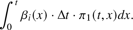 \begin{equation*} \int_0^{t} \beta_i (x)\cdot \Delta t \cdot \pi_1 (t,x) dx.\end{equation*}
 Finally, observe that  $\beta_i(x) = \beta(\xi_{1, s_1}(x))\cdot r_1 (x, \xi_{1, s_1}(x))$. Then, by substitution,
 \begin{equation*}\int_0^{t} \beta_i (x)\cdot \Delta t \cdot \pi_1 (t,x) dx
= \int_0^t \beta(\xi_{1, s_1}(x)) \cdot r_1 (x, \xi_{1, s_1}(x)) \Delta t \pi_1 (t,x) dx. \end{equation*}
\begin{equation*}\int_0^{t} \beta_i (x)\cdot \Delta t \cdot \pi_1 (t,x) dx
= \int_0^t \beta(\xi_{1, s_1}(x)) \cdot r_1 (x, \xi_{1, s_1}(x)) \Delta t \pi_1 (t,x) dx. \end{equation*}Hence, by substitution in Eqs. (A.7) and (A.8), it is obtained,
 \begin{equation*}
\pi_0 (t + \Delta t) = \pi_0 (t) - \pi_0 (t) \lambda_0 \Delta t + \pi_0 (t) o (\Delta t)+ \int_0^t \beta (\xi_{1, s_1}(x)) r_1 (x, \xi_{1, s_1}(x))\, \Delta t \, \pi_1 (t,x) dx + o (\Delta t).
\end{equation*}
\begin{equation*}
\pi_0 (t + \Delta t) = \pi_0 (t) - \pi_0 (t) \lambda_0 \Delta t + \pi_0 (t) o (\Delta t)+ \int_0^t \beta (\xi_{1, s_1}(x)) r_1 (x, \xi_{1, s_1}(x))\, \Delta t \, \pi_1 (t,x) dx + o (\Delta t).
\end{equation*}Algebraic manipulations give
 \begin{equation*}
\frac{\pi_0 (t + \Delta t) - \pi_0 (t)}{\Delta t} = -\pi_0 (t) \lambda_0 + \frac{\pi_0 (t ) o(\Delta t)}{\Delta t} + \int_0^t \beta(\xi_{1, s_1}(x))\cdot r_1 (x, \xi_{1, s_1}(x)) \, \pi_1 (t,x) dx + \frac{o(\Delta t)}{\Delta t}
\end{equation*}
\begin{equation*}
\frac{\pi_0 (t + \Delta t) - \pi_0 (t)}{\Delta t} = -\pi_0 (t) \lambda_0 + \frac{\pi_0 (t ) o(\Delta t)}{\Delta t} + \int_0^t \beta(\xi_{1, s_1}(x))\cdot r_1 (x, \xi_{1, s_1}(x)) \, \pi_1 (t,x) dx + \frac{o(\Delta t)}{\Delta t}
\end{equation*} and for  $\Delta t \to 0$, it is obtained,
 \begin{equation*}\frac{d \pi_0 (t)}{dt} = -\pi_0 (t) \lambda_0 + \int_0^t \beta(\xi_{1, s_1}(x))\cdot r_1 (x, \xi_{1, s_1}(x)) \, \pi_1 (t,x) dx,\end{equation*}
which is the first ODE composing the system of Kolmogorov forward equations.
Next the PDE for the micro-state density function  $\pi_1(t,x),\, 0 \lt x \leq t \lt \infty$ is shown. Consider the probability
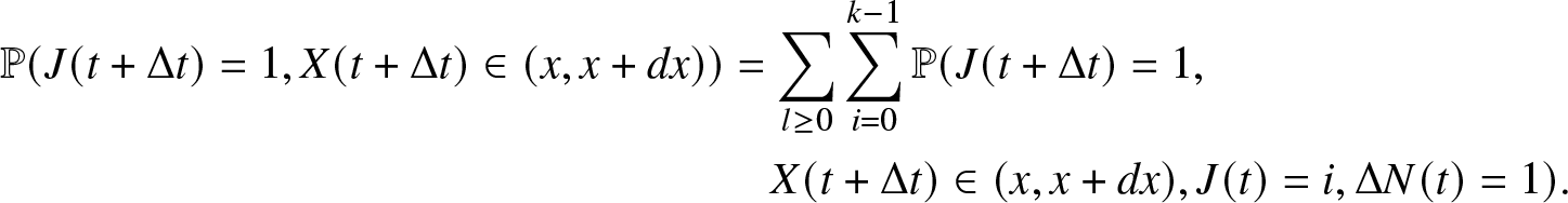 \begin{align}
\mathbb{P}(J(t + \Delta t)=1, X(t + \Delta t) \in (x, x + dx))& = \sum_{l \geq 0} \sum_{i=0}^{k-1} \mathbb{P}(J(t + \Delta t)=1, \nonumber\\
&~~~~ X(t + \Delta t) \in (x, x + dx), J(t)=i, \Delta N(t)=1).
\end{align}
\begin{align}
\mathbb{P}(J(t + \Delta t)=1, X(t + \Delta t) \in (x, x + dx))& = \sum_{l \geq 0} \sum_{i=0}^{k-1} \mathbb{P}(J(t + \Delta t)=1, \nonumber\\
&~~~~ X(t + \Delta t) \in (x, x + dx), J(t)=i, \Delta N(t)=1).
\end{align}By Lemma 3.1,the previous formula (A.11) is equal to
 \begin{align}
& = \mathbb{P}(J(t + \Delta t)=1, X(t + \Delta t) \in (x, x + dx), J(t)=0, \Delta N(t)=1)
\end{align}
\begin{align}
& = \mathbb{P}(J(t + \Delta t)=1, X(t + \Delta t) \in (x, x + dx), J(t)=0, \Delta N(t)=1)
\end{align} \begin{align}
&\qquad\qquad\qquad\qquad+ \mathbb{P}(J(t + \Delta t)=1, X(t + \Delta t) \in (x, x + dx), J(t)=1, \Delta N(t)=0)
\end{align}
\begin{align}
&\qquad\qquad\qquad\qquad+ \mathbb{P}(J(t + \Delta t)=1, X(t + \Delta t) \in (x, x + dx), J(t)=1, \Delta N(t)=0)
\end{align} \begin{align}
&\qquad\qquad\qquad\qquad+\mathbb{P}(J(t + \Delta t)=1, X(t + \Delta t) \in (x, x + dx), J(t)=2, \Delta N(t)=1) + o (\Delta t).
\end{align}
\begin{align}
&\qquad\qquad\qquad\qquad+\mathbb{P}(J(t + \Delta t)=1, X(t + \Delta t) \in (x, x + dx), J(t)=2, \Delta N(t)=1) + o (\Delta t).
\end{align} Let us consider the probability (A.12). Since the number of transitions in the interval  $(t, t + \Delta t)$ is equal to 1, $\Delta N(t) = \Delta N_f(t)=1.$ Thus,
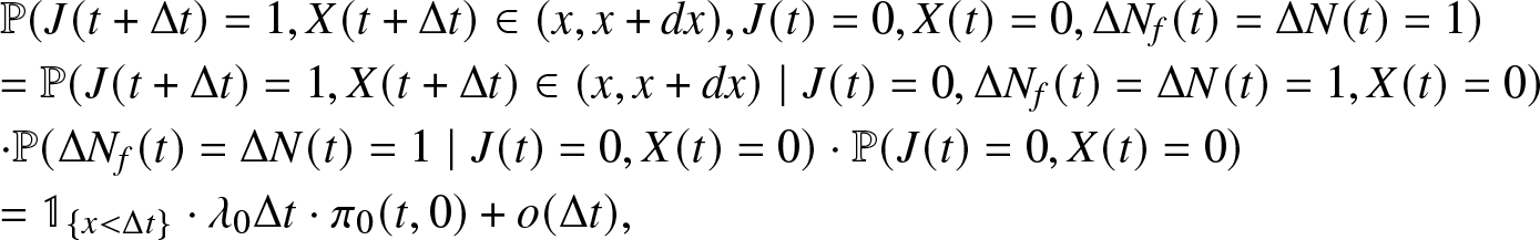 \begin{equation*}\begin{array}{l}
\mathbb{P}(J(t + \Delta t)=1, X(t + \Delta t) \in (x, x + dx), J(t)=0, X(t)=0, \Delta N_f(t)=\Delta N(t)=1) \\
= \mathbb{P}(J(t + \Delta t)=1, X(t + \Delta t) \in (x, x + dx) \mid J(t)=0, \Delta N_f(t)=\Delta N(t)=1, X(t)=0)\\
\cdot \mathbb{P}(\Delta N_f(t)=\Delta N(t)=1 \mid J(t)=0, X(t)=0) \cdot \mathbb{P}( J(t)=0, X(t)=0) \\
= \mathbb{1}_{\{x \lt \Delta t\}}\cdot \lambda_0 \Delta t \cdot \pi_0 (t,0) + o(\Delta t),
\end{array}\end{equation*}
\begin{equation*}\begin{array}{l}
\mathbb{P}(J(t + \Delta t)=1, X(t + \Delta t) \in (x, x + dx), J(t)=0, X(t)=0, \Delta N_f(t)=\Delta N(t)=1) \\
= \mathbb{P}(J(t + \Delta t)=1, X(t + \Delta t) \in (x, x + dx) \mid J(t)=0, \Delta N_f(t)=\Delta N(t)=1, X(t)=0)\\
\cdot \mathbb{P}(\Delta N_f(t)=\Delta N(t)=1 \mid J(t)=0, X(t)=0) \cdot \mathbb{P}( J(t)=0, X(t)=0) \\
= \mathbb{1}_{\{x \lt \Delta t\}}\cdot \lambda_0 \Delta t \cdot \pi_0 (t,0) + o(\Delta t),
\end{array}\end{equation*} where  $\mathbb{1}$ is the indicator function.
Next, consider probability (A.13), that is,
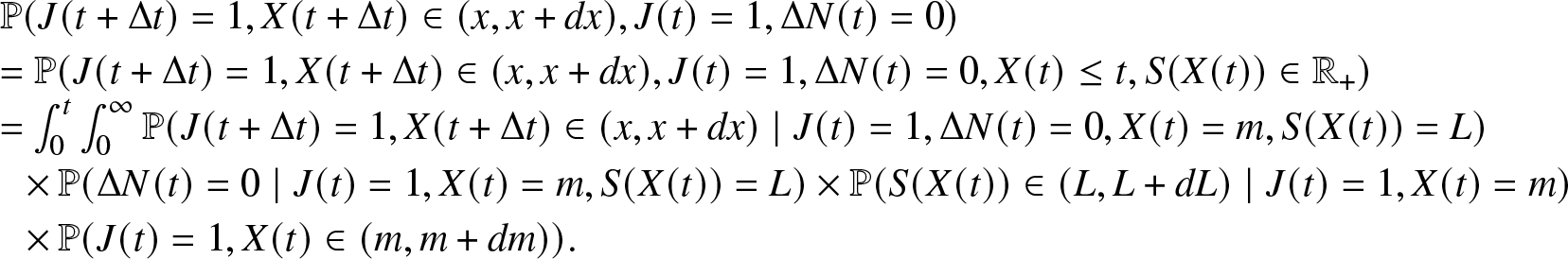 \begin{equation*}\begin{array}{l}
\mathbb{P}(J(t + \Delta t)=1, X(t + \Delta t) \in (x, x + dx), J(t)=1, \Delta N(t)=0) \\
= \mathbb{P}(J(t + \Delta t)=1, X(t + \Delta t) \in (x, x + dx), J(t)=1, \Delta N(t)=0, X(t) \leq t, S(X(t)) \in \mathbb{R_{+}})\\
= \int_0^t \int_0^{\infty} \mathbb{P}(J(t + \Delta t)=1, X(t + \Delta t) \in (x, x + dx) \mid J(t)=1, \Delta N(t)=0, X(t) = m, S(X(t)) = L) \\
\,\,\,\,\times\,\mathbb{P}( \Delta N(t) =0 \mid J(t)=1, X(t) = m, S(X(t)) = L) \times \mathbb{P}( S(X(t)) \in (L, L + dL) \mid J(t)=1, X(t) = m) \\
\,\,\,\,\times\,\mathbb{P}(J(t)=1, X(t) \in (m, m + dm)).
\end{array}\end{equation*}
\begin{equation*}\begin{array}{l}
\mathbb{P}(J(t + \Delta t)=1, X(t + \Delta t) \in (x, x + dx), J(t)=1, \Delta N(t)=0) \\
= \mathbb{P}(J(t + \Delta t)=1, X(t + \Delta t) \in (x, x + dx), J(t)=1, \Delta N(t)=0, X(t) \leq t, S(X(t)) \in \mathbb{R_{+}})\\
= \int_0^t \int_0^{\infty} \mathbb{P}(J(t + \Delta t)=1, X(t + \Delta t) \in (x, x + dx) \mid J(t)=1, \Delta N(t)=0, X(t) = m, S(X(t)) = L) \\
\,\,\,\,\times\,\mathbb{P}( \Delta N(t) =0 \mid J(t)=1, X(t) = m, S(X(t)) = L) \times \mathbb{P}( S(X(t)) \in (L, L + dL) \mid J(t)=1, X(t) = m) \\
\,\,\,\,\times\,\mathbb{P}(J(t)=1, X(t) \in (m, m + dm)).
\end{array}\end{equation*}It is just observed that for sufficiently small dm
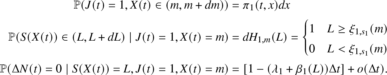 \begin{align*}
\mathbb{P}(J(t)=1, X(t) \in (m, m + dm)) &= \pi_1(t,x) dx\\
\mathbb{P}(S(X(t)) \in (L, L + dL)\mid J(t)=1, X(t) =m) &= dH_{1,m}(L) = \begin{cases}
1 & L \geq \xi_{1,s_1}(m)\\
0 & L \lt \xi_{1,s_1}(m)
\end{cases} \\
\mathbb{P}(\Delta N(t)=0 \mid S(X(t)) =L, J(t)=1, X(t) = m) &= [{1}- (\lambda_1 + \beta_1 (L)) \Delta t] + o (\Delta t).
\end{align*}
\begin{align*}
\mathbb{P}(J(t)=1, X(t) \in (m, m + dm)) &= \pi_1(t,x) dx\\
\mathbb{P}(S(X(t)) \in (L, L + dL)\mid J(t)=1, X(t) =m) &= dH_{1,m}(L) = \begin{cases}
1 & L \geq \xi_{1,s_1}(m)\\
0 & L \lt \xi_{1,s_1}(m)
\end{cases} \\
\mathbb{P}(\Delta N(t)=0 \mid S(X(t)) =L, J(t)=1, X(t) = m) &= [{1}- (\lambda_1 + \beta_1 (L)) \Delta t] + o (\Delta t).
\end{align*}By substitution and using the property of the Heaviside function, probability (A.13) becomes equal to
 \begin{equation*}\begin{array}{l}
\int_0^t \mathbb{P}(J(t + \Delta t)=1, X(t + \Delta t) \in (x, x + dx) \mid J(t)=1, \Delta N(t)=0, X(t) = m, S(X(t)) = \xi_{1,s_1}(m))\\
\times [{1}- (\lambda_1 + \beta_{1}(m))] \Delta t \, \pi_{1}(t, m) d m.
\end{array}\end{equation*}
\begin{equation*}\begin{array}{l}
\int_0^t \mathbb{P}(J(t + \Delta t)=1, X(t + \Delta t) \in (x, x + dx) \mid J(t)=1, \Delta N(t)=0, X(t) = m, S(X(t)) = \xi_{1,s_1}(m))\\
\times [{1}- (\lambda_1 + \beta_{1}(m))] \Delta t \, \pi_{1}(t, m) d m.
\end{array}\end{equation*}Further observe that
 \begin{equation*}
\beta_1(m) = \beta (\xi_{1,s_1}(m))\cdot r_1 (m, \xi_{1,s_1}(m)),
\end{equation*}
\begin{equation*}
\beta_1(m) = \beta (\xi_{1,s_1}(m))\cdot r_1 (m, \xi_{1,s_1}(m)),
\end{equation*}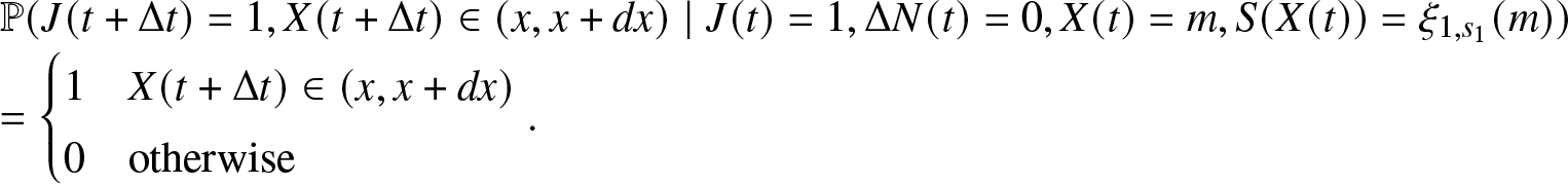 \begin{equation}
\begin{array}{l}
\mathbb{P}(J(t + \Delta t)=1, X(t + \Delta t) \in (x, x + dx) \mid J(t)=1, \Delta N(t)=0, X(t) = m, S(X(t)) = \xi_{1,s_1}(m)) \\
= \begin{cases}
1 & X(t+ \Delta t) \in (x, x+dx) \\
0 & \text{otherwise}
\end{cases}.
\end{array}
\end{equation}
\begin{equation}
\begin{array}{l}
\mathbb{P}(J(t + \Delta t)=1, X(t + \Delta t) \in (x, x + dx) \mid J(t)=1, \Delta N(t)=0, X(t) = m, S(X(t)) = \xi_{1,s_1}(m)) \\
= \begin{cases}
1 & X(t+ \Delta t) \in (x, x+dx) \\
0 & \text{otherwise}
\end{cases}.
\end{array}
\end{equation} The values of  $\Delta N(t) =0$ and $X(t) = m$ implies that the process X(t) increases linearly during the time interval $(t, t+ \Delta t)$, then $X(t + \Delta t) = m + \Delta t$. This means that probability (A.15) is equal to one only when $m + \Delta t \in (x, x+dx)$ or equivalently when $x- \Delta t \lt m \lt x - \Delta t + dx$.
These considerations allow us to represent Eq. (A.13) as
 \begin{equation*}= \int_{x- \Delta t}^{x- \Delta t + dx} [{1}- (\lambda_1 + \beta(\xi_{1,s_1}(m)) r_1(m, \xi_{1,s_1}(m)) \Delta t)] \pi_1(t, m) dm.\end{equation*}
Now, consider the probability (A.14),
 \begin{equation*}\mathbb{P}(J(t + \Delta t)=1, X(t + \Delta t) \in (x, x + dx), J(t)=2, \Delta N(t)=1).\end{equation*}
 Since, the number of transitions in  $(t, t + \Delta t)$ is equal to 1 and $J(t)=2$ and $J(t + \Delta t)=1$, the system experiences only a repair during this time interval. Hence, probability (A.14) becomes equal to
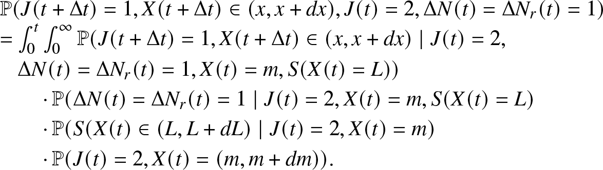 \begin{equation*}\begin{array}{l}
\mathbb{P}(J(t + \Delta t)=1, X(t + \Delta t) \in (x, x + dx), J(t)=2, \Delta N(t)=\Delta N_r(t)=1) \\
= \int_0^t \int_0^{\infty} \mathbb{P}(J(t + \Delta t)=1, X(t + \Delta t) \in (x, x + dx) \mid J(t)=2,\\
\quad\!\Delta N(t)= \Delta N_r(t)=1, X(t) = m, S(X(t)=L))\\
\qquad\cdot\,\mathbb{P}( \Delta N(t)=\Delta N_r(t)=1 \mid J(t)=2, X(t) = m, S(X(t) = L) \\
\qquad\cdot\,\mathbb{P}(S(X(t) \in (L, L+ dL) \mid J(t)=2, X(t) = m) \\
\qquad\cdot\,\mathbb{P}(J(t)=2, X(t) = (m, m + d m )).
\end{array}\end{equation*}
\begin{equation*}\begin{array}{l}
\mathbb{P}(J(t + \Delta t)=1, X(t + \Delta t) \in (x, x + dx), J(t)=2, \Delta N(t)=\Delta N_r(t)=1) \\
= \int_0^t \int_0^{\infty} \mathbb{P}(J(t + \Delta t)=1, X(t + \Delta t) \in (x, x + dx) \mid J(t)=2,\\
\quad\!\Delta N(t)= \Delta N_r(t)=1, X(t) = m, S(X(t)=L))\\
\qquad\cdot\,\mathbb{P}( \Delta N(t)=\Delta N_r(t)=1 \mid J(t)=2, X(t) = m, S(X(t) = L) \\
\qquad\cdot\,\mathbb{P}(S(X(t) \in (L, L+ dL) \mid J(t)=2, X(t) = m) \\
\qquad\cdot\,\mathbb{P}(J(t)=2, X(t) = (m, m + d m )).
\end{array}\end{equation*}It is observed that for sufficiently small dm
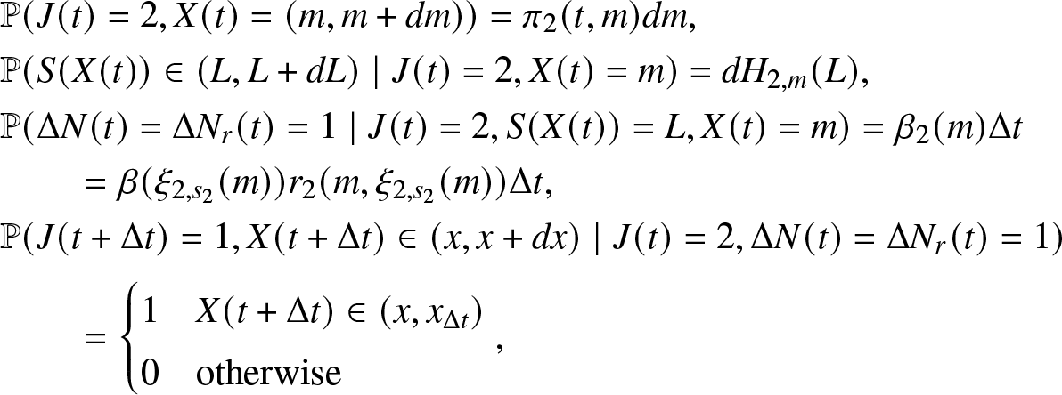 \begin{align*}
&\mathbb{P}(J(t)=2, X(t) = (m, m + d m )) = \pi_2(t, m) dm,\\
&\mathbb{P}(S( X(t)) \in (L, L + d L ) \mid J(t)=2, X(t) = m) = d H_{2,m}(L),\\
&\mathbb{P}(\Delta N(t)=\Delta N_r(t)=1 \mid J(t)=2, S(X(t))=L, X(t)=m) = \beta_2(m) \Delta t \\
&\qquad= \beta(\xi_{2, s_2}(m)) r_2 (m, \xi_{2,s_2}(m)) \Delta t,\\
&\mathbb{P}(J(t + \Delta t)=1, X(t + \Delta t) \in (x, x + dx)\mid J(t)=2, \Delta N(t)=\Delta N_r(t)=1) \\
&\qquad= \begin{cases}
1 & X(t+ \Delta t) \in (x, x_{\Delta t})\\
0 & \text{otherwise}
\end{cases},
\end{align*}
\begin{align*}
&\mathbb{P}(J(t)=2, X(t) = (m, m + d m )) = \pi_2(t, m) dm,\\
&\mathbb{P}(S( X(t)) \in (L, L + d L ) \mid J(t)=2, X(t) = m) = d H_{2,m}(L),\\
&\mathbb{P}(\Delta N(t)=\Delta N_r(t)=1 \mid J(t)=2, S(X(t))=L, X(t)=m) = \beta_2(m) \Delta t \\
&\qquad= \beta(\xi_{2, s_2}(m)) r_2 (m, \xi_{2,s_2}(m)) \Delta t,\\
&\mathbb{P}(J(t + \Delta t)=1, X(t + \Delta t) \in (x, x + dx)\mid J(t)=2, \Delta N(t)=\Delta N_r(t)=1) \\
&\qquad= \begin{cases}
1 & X(t+ \Delta t) \in (x, x_{\Delta t})\\
0 & \text{otherwise}
\end{cases},
\end{align*} where  $x_{\Delta t}:= \min\{\Delta t, x+ dx\}$ and $x \lt \Delta t$ because $X(t + \Delta t) \in (0, \Delta t)$ having a repair in the time interval
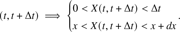 \begin{align*}(t, t+ \Delta t) \implies \begin{cases}
0 \lt X(t, t+ \Delta t) \lt \Delta t \\
x \lt X(t, t+ \Delta t) \lt x + dx \\
\end{cases}\!\!\!\!\!\!\!.\end{align*}
\begin{align*}(t, t+ \Delta t) \implies \begin{cases}
0 \lt X(t, t+ \Delta t) \lt \Delta t \\
x \lt X(t, t+ \Delta t) \lt x + dx \\
\end{cases}\!\!\!\!\!\!\!.\end{align*}Hence, by substitution,
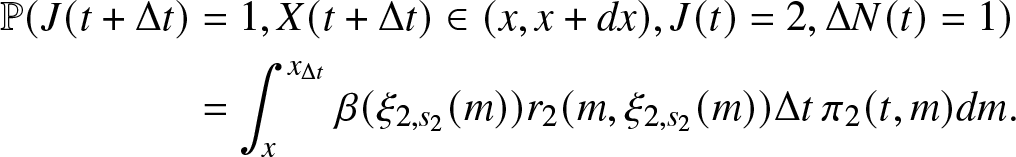 \begin{align*}
\mathbb{P}(J(t + \Delta t)&=1, X(t + \Delta t) \in (x, x + dx), J(t)=2, \Delta N(t)=1) \\
&= \int_{x}^{x_{\Delta t}} \beta (\xi_{2,s_2}(m)) r_2(m, \xi_{2,s_2}(m)) \Delta t \, \pi_2(t, m) dm.
\end{align*}
\begin{align*}
\mathbb{P}(J(t + \Delta t)&=1, X(t + \Delta t) \in (x, x + dx), J(t)=2, \Delta N(t)=1) \\
&= \int_{x}^{x_{\Delta t}} \beta (\xi_{2,s_2}(m)) r_2(m, \xi_{2,s_2}(m)) \Delta t \, \pi_2(t, m) dm.
\end{align*}Summarizing
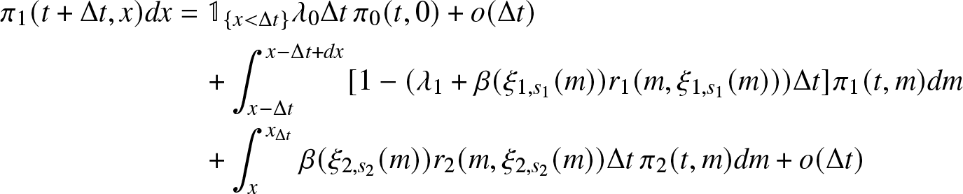 \begin{align*}
\pi_1(t+ \Delta t,x) dx &= \mathbb{1}_{\{x \lt \Delta t\}} \lambda_0 \Delta t \, \pi_0(t,0) + o(\Delta t)\\
&\quad + \int_{x-\Delta t}^{x-\Delta t+ dx} [{1}- (\lambda_1 + \beta(\xi_{1,s_1}(m)) r_1(m, \xi_{1,s_1}(m))) \Delta t] \pi_1 (t,m) d m\\
& \quad + \int_{x}^{x_{\Delta t}} \beta(\xi_{2,s_2}(m)) r_2(m, \xi_{2,s_2}(m)) \Delta t \, \pi_2 (t,m) d m + o(\Delta t)
\end{align*}
\begin{align*}
\pi_1(t+ \Delta t,x) dx &= \mathbb{1}_{\{x \lt \Delta t\}} \lambda_0 \Delta t \, \pi_0(t,0) + o(\Delta t)\\
&\quad + \int_{x-\Delta t}^{x-\Delta t+ dx} [{1}- (\lambda_1 + \beta(\xi_{1,s_1}(m)) r_1(m, \xi_{1,s_1}(m))) \Delta t] \pi_1 (t,m) d m\\
& \quad + \int_{x}^{x_{\Delta t}} \beta(\xi_{2,s_2}(m)) r_2(m, \xi_{2,s_2}(m)) \Delta t \, \pi_2 (t,m) d m + o(\Delta t)
\end{align*}which is equivalent to
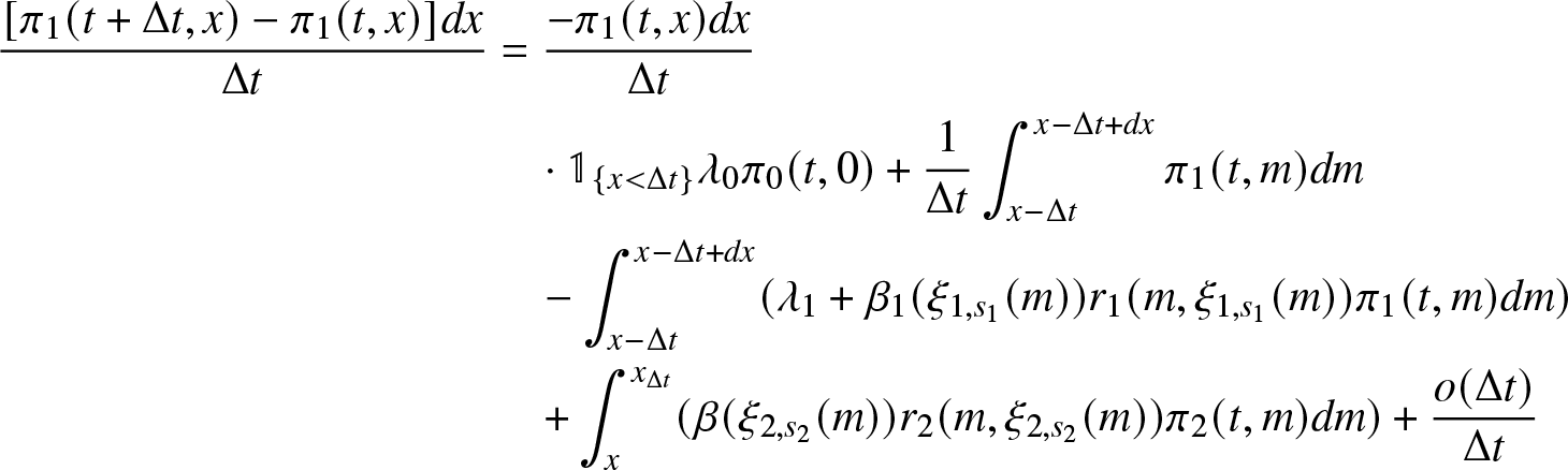 \begin{align*}
\frac{[\pi_1(t+ \Delta t,x) - \pi_1(t,x)] dx}{\Delta t} &= \frac{-\pi_1(t,x) dx}{\Delta t} \\
& \quad \cdot \mathbb{1}_{\{x \lt \Delta t\}} \lambda_0 \pi_0(t,0) + \frac{1}{\Delta t} \int_{x-\Delta t}^{x-\Delta t + dx} \pi_1(t,m) dm \\
& \quad - \int_{x-\Delta t}^{x-\Delta t + dx} (\lambda_1 + \beta_1 (\xi_{1,s_1}(m)) r_1(m, \xi_{1,s_1}(m)) \pi_1(t,m) dm) \\
&\quad + \int_{x}^{x_{\Delta t}} ( \beta (\xi_{2,s_2}(m)) r_2(m, \xi_{2,s_2}(m)) \pi_2(t,m) dm) + \frac{o(\Delta t)}{\Delta t}
\end{align*}
\begin{align*}
\frac{[\pi_1(t+ \Delta t,x) - \pi_1(t,x)] dx}{\Delta t} &= \frac{-\pi_1(t,x) dx}{\Delta t} \\
& \quad \cdot \mathbb{1}_{\{x \lt \Delta t\}} \lambda_0 \pi_0(t,0) + \frac{1}{\Delta t} \int_{x-\Delta t}^{x-\Delta t + dx} \pi_1(t,m) dm \\
& \quad - \int_{x-\Delta t}^{x-\Delta t + dx} (\lambda_1 + \beta_1 (\xi_{1,s_1}(m)) r_1(m, \xi_{1,s_1}(m)) \pi_1(t,m) dm) \\
&\quad + \int_{x}^{x_{\Delta t}} ( \beta (\xi_{2,s_2}(m)) r_2(m, \xi_{2,s_2}(m)) \pi_2(t,m) dm) + \frac{o(\Delta t)}{\Delta t}
\end{align*} for  $\Delta t \to 0$ gives
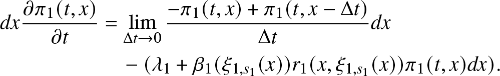 \begin{align*}
dx \frac{\partial \pi_1(t,x)}{\partial t} &= \lim_{\Delta t \to 0} \frac{-\pi_1(t,x) + \pi_1(t, x- \Delta t)}{\Delta t} dx\\
&\quad - (\lambda_1 + \beta_1 (\xi_{1,s_1}(x)) r_1(x, \xi_{1,s_1}(x)) \pi_1(t,x) dx).
\end{align*}
\begin{align*}
dx \frac{\partial \pi_1(t,x)}{\partial t} &= \lim_{\Delta t \to 0} \frac{-\pi_1(t,x) + \pi_1(t, x- \Delta t)}{\Delta t} dx\\
&\quad - (\lambda_1 + \beta_1 (\xi_{1,s_1}(x)) r_1(x, \xi_{1,s_1}(x)) \pi_1(t,x) dx).
\end{align*}Therefore,
 \begin{equation*}
\frac{\partial \pi_1 (t,x)}{\partial t} = - \frac{\partial \pi_1(t,x)}{\partial x} - (\lambda_1 + \beta_1 (\xi_{1,s_1}(x)) r_1(x, \xi_{1,s_1}(x))) \pi_1 (t,x)
\end{equation*}
\begin{equation*}
\frac{\partial \pi_1 (t,x)}{\partial t} = - \frac{\partial \pi_1(t,x)}{\partial x} - (\lambda_1 + \beta_1 (\xi_{1,s_1}(x)) r_1(x, \xi_{1,s_1}(x))) \pi_1 (t,x)
\end{equation*}or equivalently,
 \begin{equation*}
\frac{\partial \pi_1 (t,x)}{\partial t} + \frac{\partial \pi_1(t,x)}{\partial x} =- (\lambda_1 + \beta_1 (\xi_{1,s_1}(x)) r_1(x, \xi_{1,s_1}(x))) \pi_1 (t,x).
\end{equation*}
\begin{equation*}
\frac{\partial \pi_1 (t,x)}{\partial t} + \frac{\partial \pi_1(t,x)}{\partial x} =- (\lambda_1 + \beta_1 (\xi_{1,s_1}(x)) r_1(x, \xi_{1,s_1}(x))) \pi_1 (t,x).
\end{equation*} This proves the PDE for the micro-state PDF  $\pi_{1}(t,x)$.
Let us consider the PDE for the micro-state density function  $\pi_j(t,x),\, 0 \lt x \leq t \lt \infty$ and $j=2,\ldots,k-1$. Hence, using Lemma 3.1, the following representation can be provided:
 \begin{equation}
\mathbb{P}(J(t + \Delta t)=j, X(t + \Delta t) \in (x, x+dx)) = \sum_{l \geq 0} \sum_{i=0}^{k-1} \mathbb{P}(J(t + \Delta t)=j, X(t + \Delta t) \in (x, x+dx), J(t)=i, \Delta N(t)=l)
\end{equation}
\begin{equation}
\mathbb{P}(J(t + \Delta t)=j, X(t + \Delta t) \in (x, x+dx)) = \sum_{l \geq 0} \sum_{i=0}^{k-1} \mathbb{P}(J(t + \Delta t)=j, X(t + \Delta t) \in (x, x+dx), J(t)=i, \Delta N(t)=l)
\end{equation} \begin{equation}
= \mathbb{P}(J(t + \Delta t)=j, X(t + \Delta t) \in (x, x+dx), J(t)=j-1, \Delta N(t)=1)
\end{equation}
\begin{equation}
= \mathbb{P}(J(t + \Delta t)=j, X(t + \Delta t) \in (x, x+dx), J(t)=j-1, \Delta N(t)=1)
\end{equation} \begin{equation}
+ \mathbb{P}(J(t + \Delta t)=j, X(t + \Delta t) \in (x, x+dx), J(t)=j, \Delta N(t)=0)
\end{equation}
\begin{equation}
+ \mathbb{P}(J(t + \Delta t)=j, X(t + \Delta t) \in (x, x+dx), J(t)=j, \Delta N(t)=0)
\end{equation} \begin{equation}
\begin{array}{l}
= \mathbb{P}(J(t + \Delta t)=j, X(t + \Delta t) \in (x, x+dx), J(t)=j+1, \Delta N(t)=1) \\
\quad + o (\Delta t).
\end{array}
\end{equation}
\begin{equation}
\begin{array}{l}
= \mathbb{P}(J(t + \Delta t)=j, X(t + \Delta t) \in (x, x+dx), J(t)=j+1, \Delta N(t)=1) \\
\quad + o (\Delta t).
\end{array}
\end{equation} Let us consider probability (A.17). The information  $\{\Delta N(t)=1, J(t)=j-1, J(t + \Delta t)=j\}$ implies that $\Delta N(t) = \Delta N_f(t)=1$. Thus,
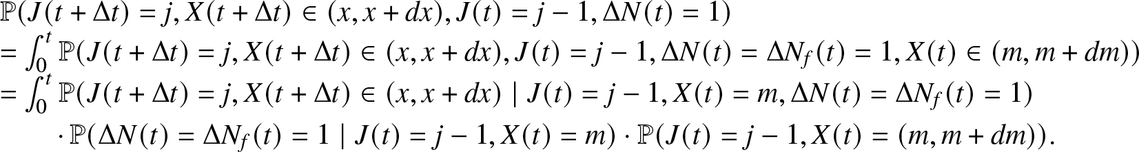 \begin{equation*}\begin{array}{l}
\mathbb{P}(J(t + \Delta t)=j, X(t + \Delta t) \in (x, x+dx), J(t)=j-1, \Delta N(t)=1) \\
= \int_0^t \mathbb{P}(J(t + \Delta t)=j, X(t + \Delta t) \in (x, x+dx), J(t)=j-1, \Delta N(t)=\Delta N_f(t)=1, X(t) \in (m, m + dm))\\
= \int_0^t \mathbb{P}(J(t + \Delta t)=j, X(t + \Delta t) \in (x, x+dx) \mid J(t)=j-1, X(t)= m, \Delta N(t)=\Delta N_f(t)=1) \\
\qquad\cdot\,\mathbb{P}( \Delta N(t)=\Delta N_f(t)=1 \mid J(t)=j-1, X(t)= m) \cdot \mathbb{P}( J(t)=j-1, X(t)= (m, m + dm)).
\end{array}\end{equation*}
\begin{equation*}\begin{array}{l}
\mathbb{P}(J(t + \Delta t)=j, X(t + \Delta t) \in (x, x+dx), J(t)=j-1, \Delta N(t)=1) \\
= \int_0^t \mathbb{P}(J(t + \Delta t)=j, X(t + \Delta t) \in (x, x+dx), J(t)=j-1, \Delta N(t)=\Delta N_f(t)=1, X(t) \in (m, m + dm))\\
= \int_0^t \mathbb{P}(J(t + \Delta t)=j, X(t + \Delta t) \in (x, x+dx) \mid J(t)=j-1, X(t)= m, \Delta N(t)=\Delta N_f(t)=1) \\
\qquad\cdot\,\mathbb{P}( \Delta N(t)=\Delta N_f(t)=1 \mid J(t)=j-1, X(t)= m) \cdot \mathbb{P}( J(t)=j-1, X(t)= (m, m + dm)).
\end{array}\end{equation*}Now, it is observed that for sufficiently small dm
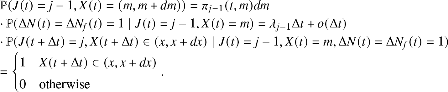 \begin{equation*}\begin{array}{l}
\mathbb{P}( J(t)=j-1, X(t)= (m, m + dm)) = \pi_{j-1}(t,m) dm \\
\cdot\,\mathbb{P}( \Delta N(t)=\Delta N_f(t)=1 \mid J(t)=j-1, X(t)= m) = \lambda_{j-1} \Delta t + o(\Delta t)\\
\cdot\,\mathbb{P}(J(t + \Delta t)=j, X(t + \Delta t) \in (x, x+dx) \mid J(t)=j-1, X(t)= m, \Delta N(t)=\Delta N_f(t)=1)\\
= \begin{cases}
1 & X(t + \Delta t) \in (x, x+ dx)\\
0 & \text{otherwise}
\end{cases}.
\end{array}\end{equation*}
\begin{equation*}\begin{array}{l}
\mathbb{P}( J(t)=j-1, X(t)= (m, m + dm)) = \pi_{j-1}(t,m) dm \\
\cdot\,\mathbb{P}( \Delta N(t)=\Delta N_f(t)=1 \mid J(t)=j-1, X(t)= m) = \lambda_{j-1} \Delta t + o(\Delta t)\\
\cdot\,\mathbb{P}(J(t + \Delta t)=j, X(t + \Delta t) \in (x, x+dx) \mid J(t)=j-1, X(t)= m, \Delta N(t)=\Delta N_f(t)=1)\\
= \begin{cases}
1 & X(t + \Delta t) \in (x, x+ dx)\\
0 & \text{otherwise}
\end{cases}.
\end{array}\end{equation*} But, it is observed that since  $\Delta N(t) = \Delta N_f(t)=1$ there is no repair, then $X(t + \Delta t) = X(t) + \Delta t = m + \Delta t$. It follows that the $\mathbb{P}(J(t + \Delta t)=j, X(t + \Delta t) \in (x, x+dx) \mid J(t)=j-1, X(t)= m, \Delta N(t)=\Delta N_f(t)=1)$ is equal to 1 only if $x \lt m + \Delta t \lt x + dx \implies x-\Delta t \lt m \lt x- \Delta t + dx$. By substitution,
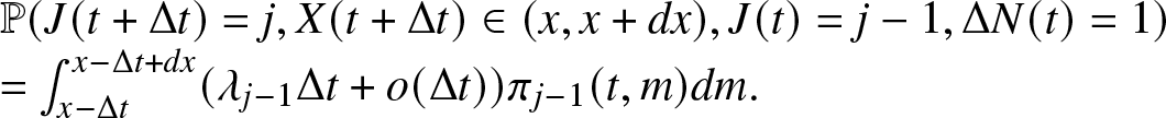 \begin{equation*}\begin{array}{l}
\mathbb{P}(J(t + \Delta t)=j, X(t + \Delta t) \in (x, x+dx), J(t)=j-1, \Delta N(t)=1)\\
= \int_{x-\Delta t}^{x-\Delta t + dx} (\lambda_{j-1} \Delta t + o(\Delta t)) \pi_{j-1}(t,m) dm.
\end{array}\end{equation*}
\begin{equation*}\begin{array}{l}
\mathbb{P}(J(t + \Delta t)=j, X(t + \Delta t) \in (x, x+dx), J(t)=j-1, \Delta N(t)=1)\\
= \int_{x-\Delta t}^{x-\Delta t + dx} (\lambda_{j-1} \Delta t + o(\Delta t)) \pi_{j-1}(t,m) dm.
\end{array}\end{equation*} Consider now the term (A.18). Since  $\Delta N(t)=0$ it means that no transition occurs during $(t, t+ \Delta t)$ and since $J(t)=j \geq 2$ the component under repair at time t will increase its time elapsed into the repair status of time $t + \Delta t$ of $\Delta t$ more time units. Hence,
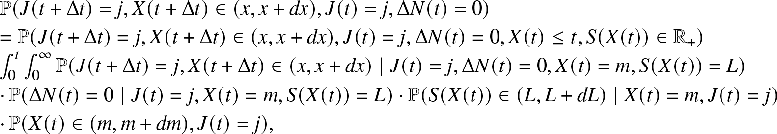 \begin{equation*}\begin{array}{l}
\mathbb{P}(J(t + \Delta t)=j, X(t + \Delta t) \in (x, x+dx), J(t)=j, \Delta N(t)=0) \\
=\mathbb{P}(J(t + \Delta t)=j, X(t + \Delta t) \in (x, x+dx), J(t)=j, \Delta N(t)=0, X(t) \leq t, S(X(t)) \in \mathbb{R_{+}})\\
\int_0^t \int_0^{\infty} \mathbb{P}(J(t + \Delta t)=j, X(t + \Delta t) \in (x, x+dx) \mid J(t)=j, \Delta N(t)=0, X(t) = m, S(X(t)) =L)\\
\cdot\,\mathbb{P}(\Delta N(t)=0 \mid J(t)=j, X(t) = m, S(X(t)) =L) \cdot \mathbb{P}(S(X(t)) \in (L, L + dL) \mid X(t) = m, J(t) =j)\\
\cdot\,\mathbb{P}(X(t) \in (m, m + dm), J(t) =j),
\end{array}\end{equation*}
\begin{equation*}\begin{array}{l}
\mathbb{P}(J(t + \Delta t)=j, X(t + \Delta t) \in (x, x+dx), J(t)=j, \Delta N(t)=0) \\
=\mathbb{P}(J(t + \Delta t)=j, X(t + \Delta t) \in (x, x+dx), J(t)=j, \Delta N(t)=0, X(t) \leq t, S(X(t)) \in \mathbb{R_{+}})\\
\int_0^t \int_0^{\infty} \mathbb{P}(J(t + \Delta t)=j, X(t + \Delta t) \in (x, x+dx) \mid J(t)=j, \Delta N(t)=0, X(t) = m, S(X(t)) =L)\\
\cdot\,\mathbb{P}(\Delta N(t)=0 \mid J(t)=j, X(t) = m, S(X(t)) =L) \cdot \mathbb{P}(S(X(t)) \in (L, L + dL) \mid X(t) = m, J(t) =j)\\
\cdot\,\mathbb{P}(X(t) \in (m, m + dm), J(t) =j),
\end{array}\end{equation*}and it is observed that for dm sufficiently small
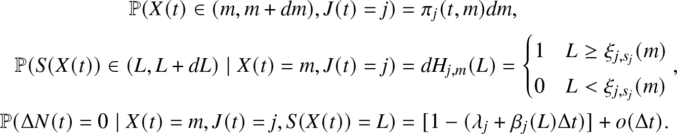 \begin{align*}
\mathbb{P}(X(t) \in (m, m + dm), J(t) =j) &= \pi_j (t, m) d m, \\
\mathbb{P}(S(X(t)) \in (L, L + dL) \mid X(t) = m, J(t) =j) &= dH_{j, m}(L) = \begin{cases}
1 & L \geq \xi_{j,s_j}(m) \\
0 & L \lt \xi_{j,s_j}(m)
\end{cases},\\
\mathbb{P}(\Delta N(t)=0 \mid X(t) = m, J(t)=j, S(X(t)) =L) &= [1- (\lambda_j + \beta_j(L) \Delta t)] + o(\Delta t).
\end{align*}
\begin{align*}
\mathbb{P}(X(t) \in (m, m + dm), J(t) =j) &= \pi_j (t, m) d m, \\
\mathbb{P}(S(X(t)) \in (L, L + dL) \mid X(t) = m, J(t) =j) &= dH_{j, m}(L) = \begin{cases}
1 & L \geq \xi_{j,s_j}(m) \\
0 & L \lt \xi_{j,s_j}(m)
\end{cases},\\
\mathbb{P}(\Delta N(t)=0 \mid X(t) = m, J(t)=j, S(X(t)) =L) &= [1- (\lambda_j + \beta_j(L) \Delta t)] + o(\Delta t).
\end{align*}By substitution,
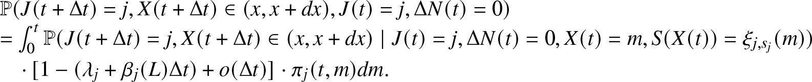 \begin{equation*}\begin{array}{l}
\mathbb{P}(J(t + \Delta t)=j, X(t + \Delta t) \in (x, x+dx), J(t)=j, \Delta N(t)=0) \\
= \int_0^t \mathbb{P}(J(t + \Delta t)=j, X(t + \Delta t) \in (x, x+dx)\mid J(t)=j, \Delta N(t)=0, X(t)=m, S(X(t)) = \xi_{j,s_j}(m)) \\
\quad\cdot\,[1- (\lambda_j + \beta_j (L) \Delta t) + o(\Delta t)] \cdot \pi_j (t, m) d m.
\end{array}\end{equation*}
\begin{equation*}\begin{array}{l}
\mathbb{P}(J(t + \Delta t)=j, X(t + \Delta t) \in (x, x+dx), J(t)=j, \Delta N(t)=0) \\
= \int_0^t \mathbb{P}(J(t + \Delta t)=j, X(t + \Delta t) \in (x, x+dx)\mid J(t)=j, \Delta N(t)=0, X(t)=m, S(X(t)) = \xi_{j,s_j}(m)) \\
\quad\cdot\,[1- (\lambda_j + \beta_j (L) \Delta t) + o(\Delta t)] \cdot \pi_j (t, m) d m.
\end{array}\end{equation*}Furthermore, observe that
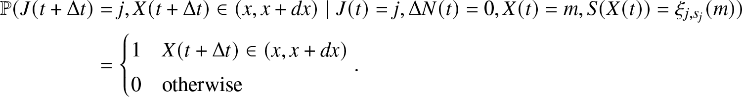 \begin{align*}
\mathbb{P}(J(t + \Delta t)&=j, X(t + \Delta t) \in (x, x+dx)\mid J(t)=j, \Delta N(t)=0, X(t)=m, S(X(t))= \xi_{j,s_j}(m)) \\
&= \begin{cases}
1 & X(t + \Delta t) \in (x, x+dx)\\
0 & \text{otherwise}
\end{cases}.
\end{align*}
\begin{align*}
\mathbb{P}(J(t + \Delta t)&=j, X(t + \Delta t) \in (x, x+dx)\mid J(t)=j, \Delta N(t)=0, X(t)=m, S(X(t))= \xi_{j,s_j}(m)) \\
&= \begin{cases}
1 & X(t + \Delta t) \in (x, x+dx)\\
0 & \text{otherwise}
\end{cases}.
\end{align*} Observe that since  $X(t) = m$ and $\Delta N(t)=0 \implies X(t + \Delta t) = m + \Delta t$ from which it follows that
 \begin{equation*}x \lt m + \Delta t \lt x + dx \implies x-\Delta t \lt m \lt x-\Delta t + dx,\end{equation*}
thus,
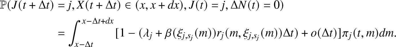 \begin{align*}
\mathbb{P}(J(t + \Delta t)&=j, X(t + \Delta t) \in (x, x+dx), J(t)=j, \Delta N(t)=0)\\
&= \int_{x-\Delta t}^{x-\Delta t+ dx} [1- (\lambda_j + \beta(\xi_{j,s_j}(m)) r_j (m, \xi_{j,s_j}(m)) \Delta t) + o(\Delta t)] \pi_j (t, m) dm.
\end{align*}
\begin{align*}
\mathbb{P}(J(t + \Delta t)&=j, X(t + \Delta t) \in (x, x+dx), J(t)=j, \Delta N(t)=0)\\
&= \int_{x-\Delta t}^{x-\Delta t+ dx} [1- (\lambda_j + \beta(\xi_{j,s_j}(m)) r_j (m, \xi_{j,s_j}(m)) \Delta t) + o(\Delta t)] \pi_j (t, m) dm.
\end{align*}Finally, the probability (A.19) is computed
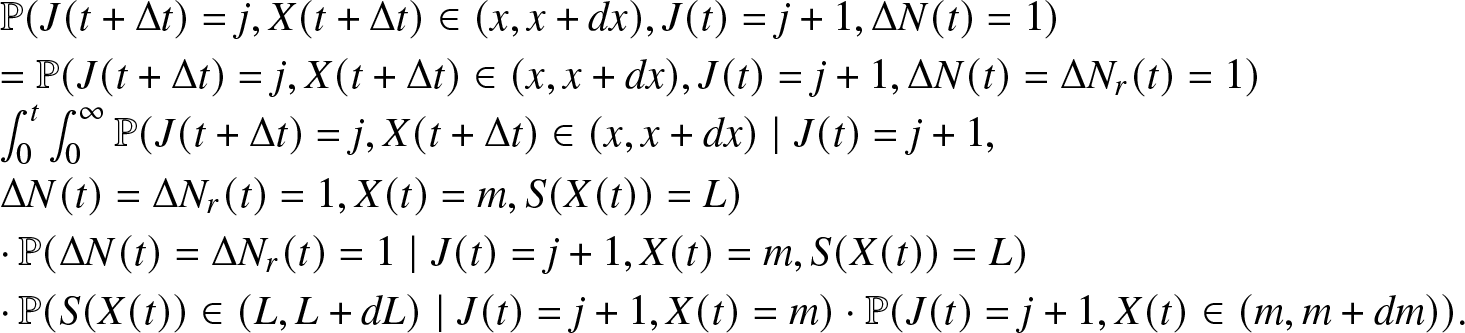 \begin{equation*}\begin{array}{l}
\mathbb{P}(J(t + \Delta t)=j, X(t + \Delta t) \in (x, x+dx), J(t)=j+1, \Delta N(t)=1) \\
= \mathbb{P}(J(t + \Delta t)=j, X(t + \Delta t) \in (x, x+dx), J(t)=j+1, \Delta N(t)=\Delta N_r(t)=1)\\
\int_0^t \int_0^{\infty} \mathbb{P}(J(t + \Delta t)=j, X(t + \Delta t) \in (x, x+dx)\mid J(t)=j+1, \\
\Delta N(t)=\Delta N_r(t)=1, X(t)=m, S(X(t))=L)\\
\cdot\,\mathbb{P}(\Delta N(t)=\Delta N_r(t)=1 \mid J(t)=j+1, X(t)=m, S(X(t))=L) \\
\cdot\,\mathbb{P}(S(X(t)) \in (L, L + dL)\mid J(t)=j+1, X(t)=m) \cdot \mathbb{P}( J(t)=j+1, X(t) \in (m, m + dm)).
\end{array}\end{equation*}
\begin{equation*}\begin{array}{l}
\mathbb{P}(J(t + \Delta t)=j, X(t + \Delta t) \in (x, x+dx), J(t)=j+1, \Delta N(t)=1) \\
= \mathbb{P}(J(t + \Delta t)=j, X(t + \Delta t) \in (x, x+dx), J(t)=j+1, \Delta N(t)=\Delta N_r(t)=1)\\
\int_0^t \int_0^{\infty} \mathbb{P}(J(t + \Delta t)=j, X(t + \Delta t) \in (x, x+dx)\mid J(t)=j+1, \\
\Delta N(t)=\Delta N_r(t)=1, X(t)=m, S(X(t))=L)\\
\cdot\,\mathbb{P}(\Delta N(t)=\Delta N_r(t)=1 \mid J(t)=j+1, X(t)=m, S(X(t))=L) \\
\cdot\,\mathbb{P}(S(X(t)) \in (L, L + dL)\mid J(t)=j+1, X(t)=m) \cdot \mathbb{P}( J(t)=j+1, X(t) \in (m, m + dm)).
\end{array}\end{equation*}Again as before, for sufficiently small dm
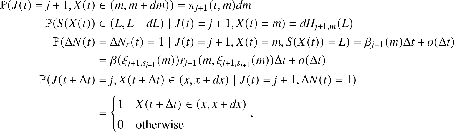 \begin{align*}
\mathbb{P}( J(t)=j+1, X(t) &\in (m, m + dm)) = \pi_{j+1}(t, m) dm\\
\mathbb{P}(S(X(t)) &\in (L, L + dL)\mid J(t)=j+1, X(t)=m) = dH_{j+1, m} (L)\\
\mathbb{P}(\Delta N(t)&=\Delta N_r(t)=1 \mid J(t)=j+1, X(t)=m, S(X(t))=L) = \beta_{j+1}(m) \Delta t + o(\Delta t) \\
&= \beta (\xi_{j+1,s_{j+1}}(m)) r_{j+1}(m, \xi_{j+1, s_{j+1}} (m)) \Delta t + o(\Delta t)\\
\mathbb{P}(J(t + \Delta t)&=j, X(t + \Delta t) \in (x, x+dx) \mid J(t)=j+1, \Delta N(t)=1) \\
&= \begin{cases}
1 & X(t+ \Delta t) \in (x, x+dx)\\
0 & \text{otherwise}
\end{cases},
\end{align*}
\begin{align*}
\mathbb{P}( J(t)=j+1, X(t) &\in (m, m + dm)) = \pi_{j+1}(t, m) dm\\
\mathbb{P}(S(X(t)) &\in (L, L + dL)\mid J(t)=j+1, X(t)=m) = dH_{j+1, m} (L)\\
\mathbb{P}(\Delta N(t)&=\Delta N_r(t)=1 \mid J(t)=j+1, X(t)=m, S(X(t))=L) = \beta_{j+1}(m) \Delta t + o(\Delta t) \\
&= \beta (\xi_{j+1,s_{j+1}}(m)) r_{j+1}(m, \xi_{j+1, s_{j+1}} (m)) \Delta t + o(\Delta t)\\
\mathbb{P}(J(t + \Delta t)&=j, X(t + \Delta t) \in (x, x+dx) \mid J(t)=j+1, \Delta N(t)=1) \\
&= \begin{cases}
1 & X(t+ \Delta t) \in (x, x+dx)\\
0 & \text{otherwise}
\end{cases},
\end{align*} where  $x_{\Delta t} = \min\{\Delta t, x+dx\}$ and $x \lt \Delta t$. But, since $ X(t + \Delta t) \in (0, \Delta t)$ and since we have a repair in $(t, t+\Delta t)$ it follows that
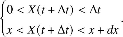 \begin{equation*}\begin{cases}
0 \lt X(t + \Delta t) \lt \Delta t \\
x \lt X(t + \Delta t) \lt x + dx
\end{cases}\!\!\!\!\!\!\!.\end{equation*}
\begin{equation*}\begin{cases}
0 \lt X(t + \Delta t) \lt \Delta t \\
x \lt X(t + \Delta t) \lt x + dx
\end{cases}\!\!\!\!\!\!\!.\end{equation*}Hence, by substitution,
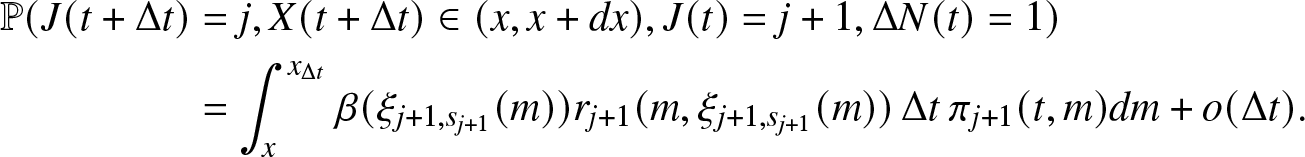 \begin{align*}
\mathbb{P}(J(t + \Delta t)&=j, X(t + \Delta t) \in (x, x+dx), J(t)=j+1, \Delta N(t)=1) \\
&= \int_{x}^{x_{\Delta t}} \beta (\xi_{j+1,s_{j+1}}(m)) r_{j+1}(m, \xi_{j+1,s_{j+1}}(m)) \, \Delta t \, \pi_{j+1} (t, m) dm + o(\Delta t).
\end{align*}
\begin{align*}
\mathbb{P}(J(t + \Delta t)&=j, X(t + \Delta t) \in (x, x+dx), J(t)=j+1, \Delta N(t)=1) \\
&= \int_{x}^{x_{\Delta t}} \beta (\xi_{j+1,s_{j+1}}(m)) r_{j+1}(m, \xi_{j+1,s_{j+1}}(m)) \, \Delta t \, \pi_{j+1} (t, m) dm + o(\Delta t).
\end{align*}Using the obtained representation for (A.17), (A.18), and (A.19),
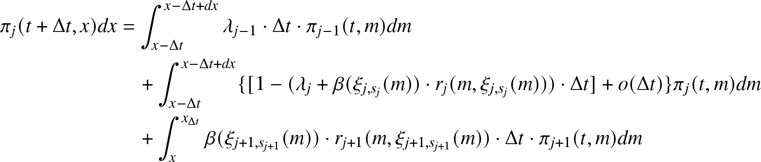 \begin{align*}
\pi_j(t+ \Delta t, x) dx & = \int_{x-\Delta t}^{x-\Delta t + dx} \lambda_{j-1} \cdot \Delta t \cdot \pi_{j-1}(t, m) dm\\
&\quad + \int_{x-\Delta t}^{x-\Delta t + dx} \{[{1}- (\lambda_j + \beta (\xi_{j,s_j}(m))\cdot r_j(m, \xi_{j,s_j}(m)))\cdot\Delta t ] + o(\Delta t) \} \pi_j(t, m) d m\\
&\quad + \int_x^{x_{\Delta t}} \beta(\xi_{j+1,s_{j+1}}(m))\cdot r_{j+1}(m, \xi_{j+1, s_{j+1}} (m))\cdot \Delta t \cdot\pi_{j+1}(t, m) d m
\end{align*}
\begin{align*}
\pi_j(t+ \Delta t, x) dx & = \int_{x-\Delta t}^{x-\Delta t + dx} \lambda_{j-1} \cdot \Delta t \cdot \pi_{j-1}(t, m) dm\\
&\quad + \int_{x-\Delta t}^{x-\Delta t + dx} \{[{1}- (\lambda_j + \beta (\xi_{j,s_j}(m))\cdot r_j(m, \xi_{j,s_j}(m)))\cdot\Delta t ] + o(\Delta t) \} \pi_j(t, m) d m\\
&\quad + \int_x^{x_{\Delta t}} \beta(\xi_{j+1,s_{j+1}}(m))\cdot r_{j+1}(m, \xi_{j+1, s_{j+1}} (m))\cdot \Delta t \cdot\pi_{j+1}(t, m) d m
\end{align*}and for sufficiently small dx,
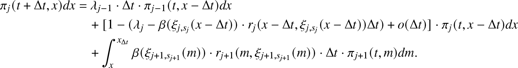 \begin{align*}
\pi_j(t+\Delta t, x) dx &= \lambda_{j-1} \cdot \Delta t \cdot \pi_{j-1} (t, x-\Delta t) dx \\
&\quad + [{1}- (\lambda_j - \beta (\xi_{j,s_j} (x-\Delta t))\cdot r_j (x-\Delta t, \xi_{j,s_{j}}(x-\Delta t)) \Delta t) + o(\Delta t)]\cdot \pi_j(t, x-\Delta t) dx \\
& \quad + \int_x^{x_{\Delta t}} \beta(\xi_{j+1,s_{j+1}}(m))\cdot r_{j+1}(m, \xi_{j+1, s_{j+1}} (m))\cdot \Delta t \cdot \pi_{j+1}(t, m) d m.
\end{align*}
\begin{align*}
\pi_j(t+\Delta t, x) dx &= \lambda_{j-1} \cdot \Delta t \cdot \pi_{j-1} (t, x-\Delta t) dx \\
&\quad + [{1}- (\lambda_j - \beta (\xi_{j,s_j} (x-\Delta t))\cdot r_j (x-\Delta t, \xi_{j,s_{j}}(x-\Delta t)) \Delta t) + o(\Delta t)]\cdot \pi_j(t, x-\Delta t) dx \\
& \quad + \int_x^{x_{\Delta t}} \beta(\xi_{j+1,s_{j+1}}(m))\cdot r_{j+1}(m, \xi_{j+1, s_{j+1}} (m))\cdot \Delta t \cdot \pi_{j+1}(t, m) d m.
\end{align*} Now, add  $-\pi_j(t,x) dx$ to both right and left hand sides of previous equation and divide by $\Delta t$ to get
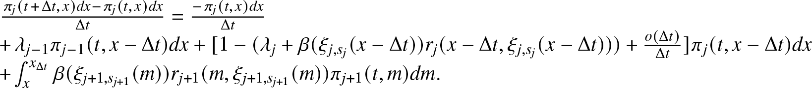 \begin{equation*}\begin{array}{l}
\frac{\pi_j(t\,+\,\Delta t,\,x) dx- \pi_j (t,\,x) dx}{\Delta t} = \frac{-\pi_j(t,\,x) dx}{\Delta t} \\
+\,\lambda_{j-1} \pi_{j-1} (t, x-\Delta t) dx + [1- (\lambda_j + \beta (\xi_{j,s_{j}}(x-\Delta t)) r_j (x-\Delta t, \xi_{j,s_j} (x-\Delta t))) + \frac{o(\Delta t)}{\Delta t}] \pi_j (t, x-\Delta t) dx \\
+ \int_x^{x_{\Delta t}} \beta(\xi_{j+1,s_{j+1}}(m)) r_{j+1} (m, \xi_{j+1,s_{j+1}}(m)) \pi_{j+1} (t, m) dm.
\end{array}\end{equation*}
\begin{equation*}\begin{array}{l}
\frac{\pi_j(t\,+\,\Delta t,\,x) dx- \pi_j (t,\,x) dx}{\Delta t} = \frac{-\pi_j(t,\,x) dx}{\Delta t} \\
+\,\lambda_{j-1} \pi_{j-1} (t, x-\Delta t) dx + [1- (\lambda_j + \beta (\xi_{j,s_{j}}(x-\Delta t)) r_j (x-\Delta t, \xi_{j,s_j} (x-\Delta t))) + \frac{o(\Delta t)}{\Delta t}] \pi_j (t, x-\Delta t) dx \\
+ \int_x^{x_{\Delta t}} \beta(\xi_{j+1,s_{j+1}}(m)) r_{j+1} (m, \xi_{j+1,s_{j+1}}(m)) \pi_{j+1} (t, m) dm.
\end{array}\end{equation*} Next, let  $\Delta t \to 0$ and observe that $\lim_{\Delta t \to 0} \int_{x}^{x_{\Delta t}}\beta(\xi_{j+1,s_{j+1}}(m)) r_{j+1} (m, \xi_{j+1,s_{j+1}}(m)) \pi_{j+1} (t, m) dm =0 $.
Therefore,
 \begin{equation*}
\frac{\partial \pi_j (t,x)}{\partial t} + \frac{\partial \pi_j (t,x)}{\partial x} = \lambda_{j-1} \pi_{j-1} (t,x) - (\lambda_j + \beta(\xi_{j,s_j}(x)) r_j (x, \xi_{j,s_j}(x)) \pi_j (t,x)).
\end{equation*}
\begin{equation*}
\frac{\partial \pi_j (t,x)}{\partial t} + \frac{\partial \pi_j (t,x)}{\partial x} = \lambda_{j-1} \pi_{j-1} (t,x) - (\lambda_j + \beta(\xi_{j,s_j}(x)) r_j (x, \xi_{j,s_j}(x)) \pi_j (t,x)).
\end{equation*} This proves the PDE for the micro-state PDF  $\pi_{j}(t,x)$ for $j=2,\ldots,K-1$.
Let us consider now the ODE for the macro-state probability  $\pi_{k}(t)$. It is first observed that
 \begin{equation*}\mathbb{P}[J(t+ \Delta t)= K, X(t + \Delta t) \in (x, x+ dx)]= \pi_k (t,x) dx = 0, \forall x \gt 0.\end{equation*}
This is due to the fact that the system is no more operational as soon as it reaches state K, thus no positive time in the repair can be considered once K components have failed.
Then consider only
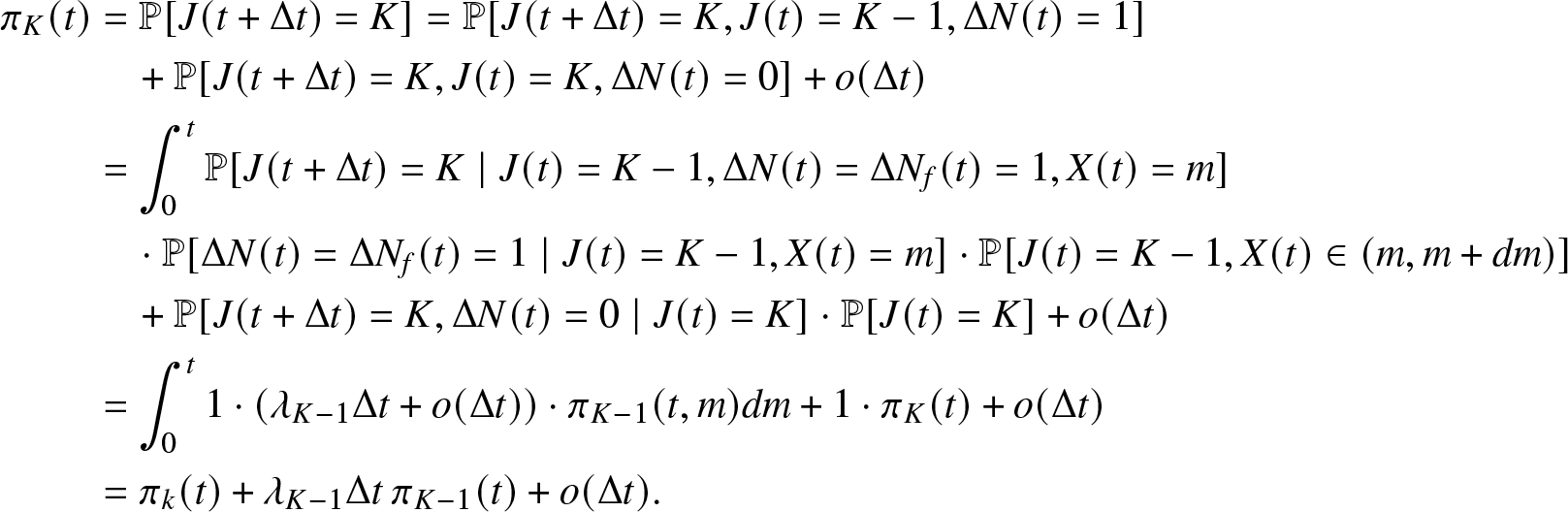 \begin{align*}
\pi_{K}(t) &= \mathbb{P}[J(t + \Delta t)=K] = \mathbb{P}[J(t+
\Delta t)=K, J(t)= K-1, \Delta N(t) =1]\\
& \quad + \mathbb{P}[J(t+\Delta t)=K, J(t)=K, \Delta N(t) = 0] + o(\Delta t)\\
&= \int_0^t \mathbb{P}[J(t+\Delta t)=K \mid J(t)=K-1, \Delta N(t) = \Delta N_f(t)= 1, X(t) = m]\\
& \quad \cdot \mathbb{P}[\Delta N(t) = \Delta N_f(t)= 1 \mid J(t)=K-1, X(t) = m] \cdot \mathbb{P}[ J(t)=K-1, X(t) \in (m, m + dm)]\\
&\quad + \mathbb{P}[J(t+\Delta t)=K, \Delta N(t)=0 \mid J(t)=K] \cdot \mathbb{P}[J(t)=K] + o(\Delta t) \\
& = \int_0^{t} {1} \cdot (\lambda_{K-1} \Delta t + o(\Delta t))\cdot \pi_{K-1} (t, m) dm + {1} \cdot \pi_K (t) + o(\Delta t)\\
&= \pi_k(t) + \lambda_{K-1} \Delta t \, \pi_{K-1} (t) + o(\Delta t).
\end{align*}
\begin{align*}
\pi_{K}(t) &= \mathbb{P}[J(t + \Delta t)=K] = \mathbb{P}[J(t+
\Delta t)=K, J(t)= K-1, \Delta N(t) =1]\\
& \quad + \mathbb{P}[J(t+\Delta t)=K, J(t)=K, \Delta N(t) = 0] + o(\Delta t)\\
&= \int_0^t \mathbb{P}[J(t+\Delta t)=K \mid J(t)=K-1, \Delta N(t) = \Delta N_f(t)= 1, X(t) = m]\\
& \quad \cdot \mathbb{P}[\Delta N(t) = \Delta N_f(t)= 1 \mid J(t)=K-1, X(t) = m] \cdot \mathbb{P}[ J(t)=K-1, X(t) \in (m, m + dm)]\\
&\quad + \mathbb{P}[J(t+\Delta t)=K, \Delta N(t)=0 \mid J(t)=K] \cdot \mathbb{P}[J(t)=K] + o(\Delta t) \\
& = \int_0^{t} {1} \cdot (\lambda_{K-1} \Delta t + o(\Delta t))\cdot \pi_{K-1} (t, m) dm + {1} \cdot \pi_K (t) + o(\Delta t)\\
&= \pi_k(t) + \lambda_{K-1} \Delta t \, \pi_{K-1} (t) + o(\Delta t).
\end{align*} Divide by  $\Delta t$ and let $\Delta t \to 0$ to get
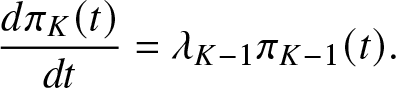 \begin{equation*}
\frac{d \pi_K(t)}{dt} = \lambda_{K-1} \pi_{K-1} (t).
\end{equation*}
\begin{equation*}
\frac{d \pi_K(t)}{dt} = \lambda_{K-1} \pi_{K-1} (t).
\end{equation*} The initial condition for  $\pi_0(0)=1$ holds true as well as the next boundary conditions
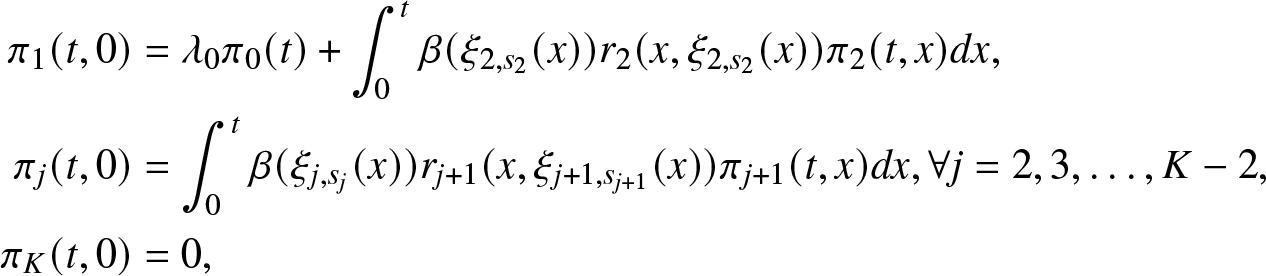 \begin{align*}
\pi_1(t,0) &= \lambda_0 \pi_0(t) + \int_0^t \beta (\xi_{2,s_2}(x)) r_2 (x, \xi_{2,s_2}(x)) \pi_2 (t,x) dx,\\
\pi_j(t,0) &= \int_0^t \beta (\xi_{j,s_j}(x)) r_{j+1} (x, \xi_{{j+1},s_{j+1}}(x)) \pi_{j+1} (t,x) dx, \forall j=2,3,\ldots,K-2,\\
\pi_K(t,0) &= 0,
\end{align*}
\begin{align*}
\pi_1(t,0) &= \lambda_0 \pi_0(t) + \int_0^t \beta (\xi_{2,s_2}(x)) r_2 (x, \xi_{2,s_2}(x)) \pi_2 (t,x) dx,\\
\pi_j(t,0) &= \int_0^t \beta (\xi_{j,s_j}(x)) r_{j+1} (x, \xi_{{j+1},s_{j+1}}(x)) \pi_{j+1} (t,x) dx, \forall j=2,3,\ldots,K-2,\\
\pi_K(t,0) &= 0,
\end{align*}which can be proved by similar arguments.
A.3. Proof of Theorem 3.8
Proof. Let us define some auxiliary concepts that shall be used in the proof. Let  $G_1^{(i)}{=} inf \{t { \gt } 0; J^{(i)}(t) =1\}$ be the random time of the first failure of the system $J^{(i)}$. Let $M_1^{(i)} = inf\{t \gt 0; J^{(i)} (G_1^{(i)} + t) \lt J^{(i)} (G_1^{(i)} + t^{-})\}$ be the random time of the first repair duration. $G_1^{(i)} + M_1^{(i)}$ is called the length of the first failure-repair (f-r) cycle. It is simple to realize that $G_1^{(i)} + M_1^{(i)}=T_{1}^{(i)}$, the time of completion of the first repair; anyway this time is splitted in the two components $G_1^{(i)}$ and $M_1^{(i)}$. The same notation applies to system (j) with obvious modification in the apex. It should be observed that during the first (f-r)-cycle the system can show any number $l \in \{1,2, \ldots, K\}$ of failures.
As a first step of the proof, another system for comparison purposes is defined and denoted by  $J^{(j_1,1)}(t)$.Footnote 1
It is assumed that it satisfies the same assumptions defining the models  $J^{(i)}$ and $J^{(j)}$ but with the following difference in the parameters:
 \begin{equation}
r_1^{(i)} (x,y) = r_1^{(j_1,1)} (x,y) \gt r_1 ^{(j)}(x,y),\, \forall x \in [0, G_1^{(j_1)} + M_1 ^{(j_1)}),\, \forall y
\end{equation}
\begin{equation}
r_1^{(i)} (x,y) = r_1^{(j_1,1)} (x,y) \gt r_1 ^{(j)}(x,y),\, \forall x \in [0, G_1^{(j_1)} + M_1 ^{(j_1)}),\, \forall y
\end{equation} \begin{equation}
r_1^{(i)} (x,y) \gt r_1^{(j_1,1)} (x,y) = r_1 ^{(j)}(x,y),\, \forall x \geq G_1^{(j_1)} + M_1 ^{(j_1)},\, \forall y
\end{equation}
\begin{equation}
r_1^{(i)} (x,y) \gt r_1^{(j_1,1)} (x,y) = r_1 ^{(j)}(x,y),\, \forall x \geq G_1^{(j_1)} + M_1 ^{(j_1)},\, \forall y
\end{equation} \begin{equation}
s_1^{(i)} = s_1^{(j_1,1)} \gt s_1^{(j)}
\end{equation}
\begin{equation}
s_1^{(i)} = s_1^{(j_1,1)} \gt s_1^{(j)}
\end{equation} \begin{equation}
r_1^{(i)} (x,y) \gt r_h^{(j_1,1)}(x,y) = r_h^{(j)} (x,y),\,\, \forall h=2,\ldots,k-1, \forall x,y
\end{equation}
\begin{equation}
r_1^{(i)} (x,y) \gt r_h^{(j_1,1)}(x,y) = r_h^{(j)} (x,y),\,\, \forall h=2,\ldots,k-1, \forall x,y
\end{equation} \begin{equation}
s_1^{(i)} \gt s_h^{(j_1,1)} = s_h^{(j)}, \,\,\forall h=2,\ldots,k-1.
\end{equation}
\begin{equation}
s_1^{(i)} \gt s_h^{(j_1,1)} = s_h^{(j)}, \,\,\forall h=2,\ldots,k-1.
\end{equation} With this specification, the model  $J^{(j_1,1)}$ differs of system $J^{(j)}$ up to the completion of the first (f-r)-cycle being characterized by larger values of the effort rate function and initial effort. Once the first (f-r)-cycle of $J^{(j_1,1)}$ is completed, this system behaves as $J^{(j)}$ in the probabilistic sense. A direct inspection of relations (A.20–A.24) shows that the system $J^{(j_1,1)}$ is a probabilistic copy of system $J^{(i)}$ up to the completion of the first (f-r)-cycle sharing the same values of the effort rate functions and initial effort. Once the first (f-r)-cycle of $J^{(j_1,1)}$ is completed, this system has small values of the effort rate function and initial effort as compared to $J^{(i)}$.
As a second step, the notation is introduced:
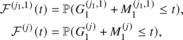 \begin{align*}
\mathcal{F}^{(j_1,1)}(t)& = \mathbb{P}(G_1^{(j_1,1)} + M_1^{(j_1,1)} \leq t), \\
\mathcal{F}^{(j)}(t)& = \mathbb{P}(G_1^{(j)} + M_1^{(j)} \leq t),
\end{align*}
\begin{align*}
\mathcal{F}^{(j_1,1)}(t)& = \mathbb{P}(G_1^{(j_1,1)} + M_1^{(j_1,1)} \leq t), \\
\mathcal{F}^{(j)}(t)& = \mathbb{P}(G_1^{(j)} + M_1^{(j)} \leq t),
\end{align*} for the CDF’s of the first (f-r)-cycle duration and the following is going to be proved  $\mathcal{F}^{(j_1,1)}(t) \geq \mathcal{F}^{(j)}(t), \forall t \in \mathbb{R_{+}}$. Indeed,
 \begin{equation*}
\mathcal{F}^{(j_1,1)}(t) = \int_0^t \mathbb{P} (M_1^{(j_1,1)} \leq t - G_1^{(j_1,1)} \mid G_1^{(j_1,1)} = g_1)\cdot \mathbb{P} (G_1^{(j_1,1)} \in (g_1, g_1 + dg_1)),
\end{equation*}
\begin{equation*}
\mathcal{F}^{(j_1,1)}(t) = \int_0^t \mathbb{P} (M_1^{(j_1,1)} \leq t - G_1^{(j_1,1)} \mid G_1^{(j_1,1)} = g_1)\cdot \mathbb{P} (G_1^{(j_1,1)} \in (g_1, g_1 + dg_1)),
\end{equation*}and it is observed that
 \begin{equation*} \mathbb{P} (G_1^{(j_1,1)} \in (g_1, g_1 + dg_1)) = dF_{G}^{(j_1,1)} (g_1) = dF_G^{(j)} (g_1)\end{equation*}
 in virtue of the fact that the systems  $J^{(j_1,1)}$ and $J^{(j)}$ are different only in the repair force related to the first (f-r)-cycle and not in the failure mechanism. Further, it is observed that the random variable $M_1^{(j_1,1)}$ is independent of $G_1^{(j_1,1)}$ and its failure rate is
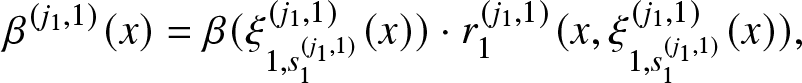 \begin{equation*}\beta^{(j_1,1)} (x) = \beta(\xi^{(j_1,1)}_{1,s_1^{(j_1,1)}}(x))\cdot r_1^{(j_1,1)}(x, \xi_{1,s_1^{(j_1,1)}}^{(j_1,1)} (x)),
\end{equation*}
\begin{equation*}\beta^{(j_1,1)} (x) = \beta(\xi^{(j_1,1)}_{1,s_1^{(j_1,1)}}(x))\cdot r_1^{(j_1,1)}(x, \xi_{1,s_1^{(j_1,1)}}^{(j_1,1)} (x)),
\end{equation*}while
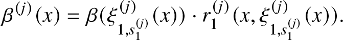 \begin{equation*} \beta^{(j)}(x) = \beta(\xi^{(j)}_{1,s_1^{(j)}}(x))\cdot r_1^{(j)}(x, \xi_{1,s_1^{(j)}}^{(j)} (x)). \end{equation*}
 From relation (A.20), being  $r_1^{(j_1,1)} (\cdot,\cdot) \gt r_1^{(j)}(\cdot,\cdot)$ and $s_1^{(j_1,1)} \gt s_1^{(j)}$, $\xi^{(j_1,1)}_{1,s_1^{(j_1,1)}}(x)) \gt \xi^{(j)}_{1,s_1^{(j)}}(x)) $ which in turn implies
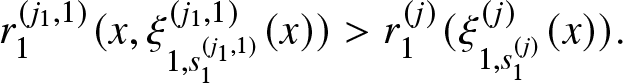 \begin{equation*}r_1^{(j_{1},1)} (x, \xi^{(j_1,1)}_{1,s_1^{(j_1,1)}}(x)) \gt r_1^{(j)} (\xi^{(j)}_{1,s_1^{(j)}}(x)). \end{equation*}
Moreover, since the CDF of the base repair mechanism is increasing hazard rate,
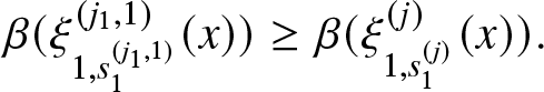 \begin{equation*}\beta(\xi^{(j_1,1)}_{1,s_1^{(j_1,1)}}(x)) \geq \beta(\xi^{(j)}_{1,s_1^{(j)}}(x)).\end{equation*}
 Then,  $\forall x, \beta^{(j_1,1)} (x) \geq \beta^{(j)}(x)$, which means that $M_1^{(j_1,1)} \geq_{h_r} M_1^{(j)} \implies M_1^{(j_1,1)} \leq_{FSD} M_1^{(j)} \iff \mathcal{F}^{(j_1,1)}(t) \geq \mathcal{F}^{(j)}(t).$
The third step of the proof consists of the comparison of the reliability functions. Consider any  $k\in \{0,1,\ldots,K-1\}$ and the probability
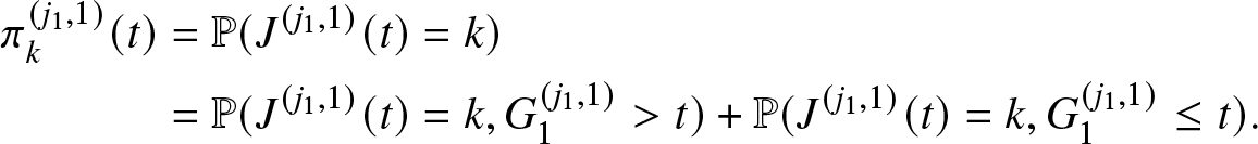 \begin{align*}
\pi_k^{(j_1,1)} (t) & = \mathbb{P} (J^{(j_1,1)} (t)= k)\\
& = \mathbb{P} (J^{(j_1,1)} (t)=k, G_1^{(j_1,1)} \gt t) + \mathbb{P} (J^{(j_1,1)} (t) = k, G_1^{(j_1,1)} \leq t).
\end{align*}
\begin{align*}
\pi_k^{(j_1,1)} (t) & = \mathbb{P} (J^{(j_1,1)} (t)= k)\\
& = \mathbb{P} (J^{(j_1,1)} (t)=k, G_1^{(j_1,1)} \gt t) + \mathbb{P} (J^{(j_1,1)} (t) = k, G_1^{(j_1,1)} \leq t).
\end{align*}Introduce the notation
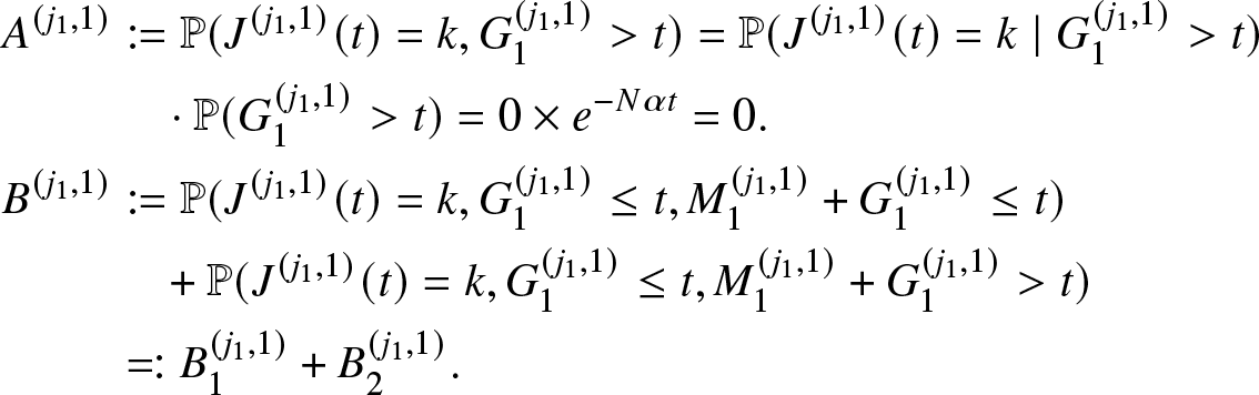 \begin{align*}
A^{(j_1,1)} & := \mathbb{P}(J^{(j_1,1)} (t)=k, G_1^{(j_1,1)} \gt t) = \mathbb{P}(J^{(j_1,1)} (t)=k \mid G_1^{(j_1,1)} \gt t) \\
&\quad \cdot \mathbb{P}(G_1^{(j_1,1)} \gt t) =0 \times e^{-N \alpha t} = 0.\\
B^{(j_1,1)} & := \mathbb{P} (J^{(j_1,1)} (t) = k, G_1^{(j_1,1)} \leq t, M_1^{(j_1,1)} + G_1^{(j_1,1)} \leq t) \\
&\quad + \mathbb{P} (J^{(j_1,1)} (t) = k, G_1^{(j_1,1)} \leq t, M_1^{(j_1,1)} + G_1^{(j_1,1)} \gt t)\\
& =: B_{1}^{(j_1,1)}+B_{2}^{(j_1,1)}.
\end{align*}
\begin{align*}
A^{(j_1,1)} & := \mathbb{P}(J^{(j_1,1)} (t)=k, G_1^{(j_1,1)} \gt t) = \mathbb{P}(J^{(j_1,1)} (t)=k \mid G_1^{(j_1,1)} \gt t) \\
&\quad \cdot \mathbb{P}(G_1^{(j_1,1)} \gt t) =0 \times e^{-N \alpha t} = 0.\\
B^{(j_1,1)} & := \mathbb{P} (J^{(j_1,1)} (t) = k, G_1^{(j_1,1)} \leq t, M_1^{(j_1,1)} + G_1^{(j_1,1)} \leq t) \\
&\quad + \mathbb{P} (J^{(j_1,1)} (t) = k, G_1^{(j_1,1)} \leq t, M_1^{(j_1,1)} + G_1^{(j_1,1)} \gt t)\\
& =: B_{1}^{(j_1,1)}+B_{2}^{(j_1,1)}.
\end{align*}They can be computed as follows:
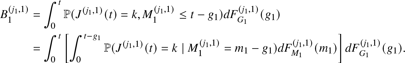 \begin{align*}
B_1^{(j_1,1)} &= \int_0^t \mathbb{P}(J^{(j_1,1)}(t) = k, M_1^{(j_1,1)} \leq t-g_1) d F_{G_1}^{(j_1,1)}(g_1)\\
& = \int_0^t \left[ \int_0^{t-g_1} \mathbb{P}(J^{(j_1,1)} (t) = k \mid M_1^{(j_1,1)} = m_1-g_1) dF_{M_1}^{(j_1,1)} (m_1)\right] dF_{G_1}^{(j_1,1)}(g_1).
\end{align*}
\begin{align*}
B_1^{(j_1,1)} &= \int_0^t \mathbb{P}(J^{(j_1,1)}(t) = k, M_1^{(j_1,1)} \leq t-g_1) d F_{G_1}^{(j_1,1)}(g_1)\\
& = \int_0^t \left[ \int_0^{t-g_1} \mathbb{P}(J^{(j_1,1)} (t) = k \mid M_1^{(j_1,1)} = m_1-g_1) dF_{M_1}^{(j_1,1)} (m_1)\right] dF_{G_1}^{(j_1,1)}(g_1).
\end{align*} Let us denote by  $k^{(j_1,1)} (m_1) := \mathbb{P} (J^{(j_1,1)} (t) = k \mid M_1^{(j_1,1)} = m_1-g_1)$ and observe that this function is increasing in m 1. Additionally, due to the fact that after the completion of the first (f-r)-cycle the two systems are probabilistically identical, it is observed that $k^{(j_1,1)} (m_1) = k^{(j)}(m_1)$. Hence, being $F_{M_1}^{(j_1,1)}(\cdot) \geq F_{M_1}^{(j)} (\cdot)$ because $\mathcal{F}^{(j_1,1)}(\cdot) \geq \mathcal{F}^{(j)}(\cdot)$ and $F_{G_1}^{(j_1,1)}(\cdot) = F_{G_1}^{(j)}(\cdot)$ it follows that
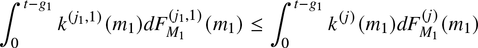 \begin{equation*}\int_0^{t-g_1} k^{(j_1,1)}(m_1) dF_{M_1}^{(j_1,1)} (m_1) \leq \int_0^{t-g_1} k^{(j)}(m_1) dF_{M_1}^{(j)} (m_1)\end{equation*}
and then
 \begin{equation*}\int_{0}^{t}\Bigg[\int_0^{t-g_1} k^{(j_1,1)}(m_1)dF_{M_1}^{(j_1,1)} (m_1)\Bigg] dF_{G_1}^{(j_1,1)} (g_1) \leq \int_{0}^{t}\Bigg[\int_0^{t-g_1} k^{(j)}(m_1) dF_{M_1}^{(j)} (m_1)\Bigg] dF_{G_1}^{(j)} (g_1).\end{equation*}
 This proves that  $B_1^{(j_1,1)} \leq B_1^{(j)}$. Consider now the probability $B_2^{(j_1,1)}$,
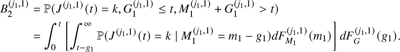 \begin{align*}
B_2^{(j_1,1)} & = \mathbb{P}(J^{(j_1,1)} (t)=k, G_1^{(j_1,1)} \leq t, M_1^{(j_1,1)} + G_1^{(j_1,1)} \gt t )\\
& = \int_0^t \left[ \int_{t-g_1}^{\infty} \mathbb{P} (J^{(j_1,1)}(t) = k \mid M_1^{(j_1,1)} = m_1-g_1 ) dF_{M_1}^{(j_1,1)} (m_1) \right] dF_G^{(j_1,1)}(g_1).
\end{align*}
\begin{align*}
B_2^{(j_1,1)} & = \mathbb{P}(J^{(j_1,1)} (t)=k, G_1^{(j_1,1)} \leq t, M_1^{(j_1,1)} + G_1^{(j_1,1)} \gt t )\\
& = \int_0^t \left[ \int_{t-g_1}^{\infty} \mathbb{P} (J^{(j_1,1)}(t) = k \mid M_1^{(j_1,1)} = m_1-g_1 ) dF_{M_1}^{(j_1,1)} (m_1) \right] dF_G^{(j_1,1)}(g_1).
\end{align*}Also, in this case
 \begin{equation}
k^{(j_1,1)}(m_1):= \mathbb{P} (J^{(j_1,1)}(t)=k \mid M_1^{(j_1,1)} = m_1-g_1)
\end{equation}
\begin{equation}
k^{(j_1,1)}(m_1):= \mathbb{P} (J^{(j_1,1)}(t)=k \mid M_1^{(j_1,1)} = m_1-g_1)
\end{equation} \begin{equation}
\qquad\qquad\qquad\qquad=\mathbb{P} (J^{(j)} (t) = k \mid M_1^{(j)} = m_1-g_1)= k^{(j)}(m_1),
\end{equation}
\begin{equation}
\qquad\qquad\qquad\qquad=\mathbb{P} (J^{(j)} (t) = k \mid M_1^{(j)} = m_1-g_1)= k^{(j)}(m_1),
\end{equation}and both are increasing in m 1. Hence,
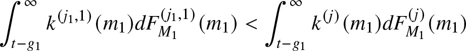 \begin{equation*}\int_{t-g_1}^{\infty} k^{(j_1,1)}(m_1) dF_{M_1}^{(j_1,1)}(m_1) \lt \int_{t-g_1}^{\infty} k^{(j)}(m_1) dF_{M_1}^{(j)}(m_1)\end{equation*}
 because  $F_{M_1}^{(j_1,1)}(\cdot) \geq F_{M_1}^{(j)}(\cdot)$. This implies (from the equality of $F_{G_1}^{(j_1,1)}(\cdot) = F_{G_1}^{(j)}(\cdot)$) that $B_2^{(j_1,1)} \leq B_2^{(j)}$. Then, it is obtained that
 \begin{equation*}\pi_k^{(j_1,1)}(t) = B_1^{(j_1,1)} + B_2^{(j_1,1)} \leq B_1^{(j)} + B_2^{(j)} = \pi_k^{(j)}(t)\end{equation*}
and
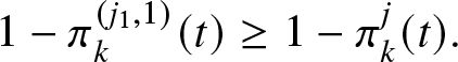 \begin{equation*}1- \pi_k^{(j_1,1)}(t) \geq 1 - \pi_k^{j} (t).\end{equation*}
 Hence, the proof is complete as even only the differences in the effort rate functions and to their initial values confined to the first (f-r)-cycle determines  $R^{(j_1,1)} (t) \geq R^{(j)}$. Then, $R^{(i)} (t) \geq R^{(j)} (t)$ as the $J^{(i)}$ system may have infinite (f-r)-cycles.


 Open access