


1. Introduction
It is well-known that entropy and divergence measures play a pivotal role in different fields of science and technology. For example, in coding theory, Farhadi and Charalambous [Reference Farhadi and Charalambous7] used the concept of entropy for robust coding in a class of sources. In statistical mechanics, Kirchanov [Reference Kirchanov24] adopted generalized entropy to describe quantum dissipative systems. In economics, Rohde [Reference Rohde34] made use of the J-divergence measure to study economic inequality. An important generalization of the Shannon entropy is the Rényi entropy, which also unifies other entropies like the min-entropy or collision entropy. Consider two absolutely continuous non-negative random variables X and Y with respective probability density functions (PDFs)  $f(\cdot)$ and $g(\cdot)$. Henceforth, the random variables are considered to be non-negative and absolutely continuous, unless otherwise stated. The Rényi entropy of X and Rényi divergence between X and Y are, respectively, given by (see [Reference Rényi33])
 \begin{align}
H_\alpha(X)=\delta(\alpha)\log\int_{0}^{\infty}f^\alpha(x)dx~ \text
{and}~ RD^\alpha(X,Y)=\delta^*(\alpha)\log\int_{0}^{\infty}f^\alpha(x)g^{1-\alpha}(x)dx,
\end{align}
\begin{align}
H_\alpha(X)=\delta(\alpha)\log\int_{0}^{\infty}f^\alpha(x)dx~ \text
{and}~ RD^\alpha(X,Y)=\delta^*(\alpha)\log\int_{0}^{\infty}f^\alpha(x)g^{1-\alpha}(x)dx,
\end{align} where  $\delta(\alpha)=\frac{1}{1-\alpha}$, $\delta^*(\alpha)=\frac{1}{\alpha-1}$, $0 \lt \alpha \lt \infty,~\alpha\ne1$. Throughout the paper, “log” is used to denote the natural logarithm. It can be easily established that when $\alpha\rightarrow1$, the Rényi entropy and Rényi divergence reduce to the Shannon entropy (see [Reference Shannon40]) and Kullback–Leibler (KL)-divergence (see [Reference Kullback and Leibler25]), respectively, given by
 \begin{align}
H(X)=-\int_{0}^{\infty}f(x)\log f(x)dx~ \text
{and}~ KL(X,Y)=\int_{0}^{\infty}f(x)\log\frac{f(x)}{g(x)}dx.
\end{align}
\begin{align}
H(X)=-\int_{0}^{\infty}f(x)\log f(x)dx~ \text
{and}~ KL(X,Y)=\int_{0}^{\infty}f(x)\log\frac{f(x)}{g(x)}dx.
\end{align} In distribution theory, properties like mean, variance, skewness, and kurtosis are extracted using successive moments of a probability distribution, which are obtained by taking successive derivatives of the moment-generating function at the origin. Likewise, the information generating functions (IGFs) for probability distributions are constructed in order to compute many information quantities like the KL-divergence and Shannon entropy. In Physics and Chemistry, the non-extensive thermodynamics and chaos theory depend on the IGF, also referred to as the entropic moment. In 1966, Golomb [Reference Golomb11] introduced the IGF and showed that its first-order derivative at 1 yields negative Shannon entropy. For a random variable X with PDF  $f(\cdot)$, the Golomb’s IGF, for γ > 0, is defined as
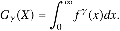 \begin{align}
G_\gamma(X)=\int_{0}^{\infty}f^\gamma(x)dx.
\end{align}
\begin{align}
G_\gamma(X)=\int_{0}^{\infty}f^\gamma(x)dx.
\end{align} It is clear that  $G_\gamma(X)\big|_{\gamma=1}=1$ and $\frac{d}{d\gamma}G_\gamma(X)\big|_{\gamma=1}=-H(X)$. Again, for γ = 2, the IGF in (1.3) reduces to the Onicescu’s informational energy (IE) (see [Reference Onicescu30]), given by
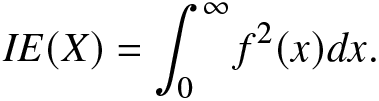 \begin{eqnarray}
IE(X)=\int_{0}^{\infty}f^2(x)dx.
\end{eqnarray}
\begin{eqnarray}
IE(X)=\int_{0}^{\infty}f^2(x)dx.
\end{eqnarray}The IE has many applications in different fields; for example, IE is used as a correlation measure in systems of atoms and molecules (see [Reference Flores-Gallegos9]), and highly correlated Hylleraas wave functions in the analysis of the ground state helium (see [Reference Ou and Ho31]). Later, motivated by the Golomb’s IGF, Guiasu and Reischer [Reference Guiasu and Reischer13] proposed relative IGF. For random variables X and Y, the relative IGF, for θ > 0, is given by
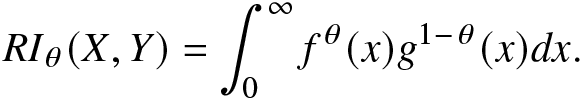 \begin{align*}
RI_\theta(X,Y)=\int_{0}^{\infty}f^\theta(x)g^{1-\theta}(x)dx.
\end{align*}
\begin{align*}
RI_\theta(X,Y)=\int_{0}^{\infty}f^\theta(x)g^{1-\theta}(x)dx.
\end{align*} Apparently,  $RI_\theta(X,Y)|_{\theta=1}=1$ and $\frac{d}{d\theta}RI_\theta(X,Y)|_{\theta=1}=KL(X,Y)$. Recently, the IGFs have been studied in great detail due to their capability of generating various useful uncertainty and divergence measures.
Kharazmi and Balakrishnan [Reference Kharazmi and Balakrishnan18] introduced Jensen IGF and IGF for a residual lifetime and discussed their important properties. Kharazmi and Balakrishnan [Reference Kharazmi and Balakrishnan19] introduced a generating function for the generalized Fisher information and established various results using it. Kharazmi and Balakrishnan [Reference Kharazmi and Balakrishnan20] proposed cumulative residual IGF and relative cumulative residual IGF. In addition to these, one may also refer to [Reference Kharazmi and Balakrishnan17, Reference Kharazmi, Balakrishnan and Ozonur21, Reference Kharazmi, Contreras-Reyes and Balakrishnan23, Reference Smitha and Kattumannil41, Reference Smitha, Kattumannil and Sreedevi42, Reference Zamani, Kharazmi and Balakrishnan44] and [Reference Capaldo, Di Crescenzo and Meoli4] for more work on generating functions. Recently, Saha and Kayal [Reference Saha and Kayal37] proposed general-weighted IGF and general-weighted relative IGF and developed some associated results.
Motivated by the usefulness of the previously introduced IGFs as described above, we develop here some IGFs and explore their properties. We mention that the IGFs with utilities were introduced earlier by Jain and Srivastava [Reference Jain and Srivastava16] only for discrete cases. In this paper, we mainly focus on the generalized versions of the IGFs in the continuous framework. The key contributions made here are described below:
• In Section 2, we propose the Rényi information generating function (RIGF) for both discrete and continuous random variables and discuss various properties. For discrete distributions, a relation between the RIGF and the Hill number (a diversity index) is obtained. The RIGF is expressed in terms of the Shannon entropy of order q > 0. We also obtain a bound for RIGF. The RIGF is then evaluated for escort distributions.
• In Section 3, we introduced the Rényi divergence information generating function (RDIGF). The relation between the RDIGF of generalized escort distributions is evaluated, the RDIGF and RIGF of baseline distributions is then established. Further, the RDIGF is examined under strictly monotone transformations.
• In Section 4, we propose nonparametric and parametric estimators of the proposed RIGF and IGF according to [Reference Golomb11]. A Monte Carlo simulation study is carried out for both these estimators. Further, the nonparametric and parametric estimators are compared on the basis of standard deviation (SD), absolute bias (AB), and mean square error (MSE) for the case of Weibull distribution. A real dataset is considered and analyzed finally in Section 5.
• Section 6 discusses some applications of the proposed generating functions. The RIGF is studied for coherent systems. Several properties including bounds are obtained. In particular, three coherent systems are considered, and then the numerical values of RIGF, IGF, Rényi entropy, and varentropy are computed for them. It is observed that the proposed measure can be considered as an alternative uncertainty measure since it has a similar behavior as other well-established information measures. Further, we have established that the RDIGF and RIGF can be considered as effective tools for model selection. Furthermore, three chaotic maps, namely, logistic map, Chebyshev map, and Hénnon map, have been considered for the validation of the proposed IGF. Finally, Section 7 presents some concluding remarks.
Throughout the paper, all the integrations and differentiations involved are assumed to exist.
2. Rényi information generating functions
We propose RIGFs for discrete and continuous random variables and discuss some of their properties. First, we present RIGF for a discrete random variable. Hereafter,  $\mathbb{N}$ is used to denote the set of natural numbers.
Definition 2.1. Suppose X is a discrete random variable taking values  $x_i,$ for $i=1,\dots,n\in\mathbb{N}$ with PMF $P(X=x_i)=p_i \gt 0$, $\sum_{i=1}^{n}p_{i}=1$. Then, the RIGF of X is defined as
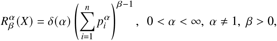 \begin{align}
R^\alpha_\beta(X)=\delta(\alpha)\left(\sum_{i=1}^{n}p_i^\alpha\right)^{\beta-1},~~0 \lt \alpha \lt \infty,~ \alpha\neq1,~ \beta \gt 0,
\end{align}
\begin{align}
R^\alpha_\beta(X)=\delta(\alpha)\left(\sum_{i=1}^{n}p_i^\alpha\right)^{\beta-1},~~0 \lt \alpha \lt \infty,~ \alpha\neq1,~ \beta \gt 0,
\end{align} where  $\delta(\alpha)=\frac{1}{1-\alpha}$.
Clearly,  $R_\beta^\alpha(X)|_{\beta=1}=\delta(\alpha)$ and
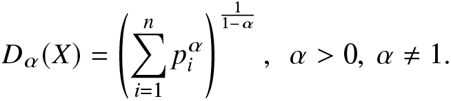
  $R_\beta^\alpha(X)|_{\beta=2,\alpha=2}=-\sum_{i=1}^{n}p_{i}^2=-S$, where S is known as the Simpson’s index (see [Reference Gress and Rosenberg12]). We recall that the Simpson’s index is useful in ecology to quantify the biodiversity of a habitant. In addition, the proposed RIGF given in (2.1) can be connected with the Hill number (see [Reference Hill15]), which is also an important diversity index employed by many researchers in ecology (see [Reference Chao, Chiu and Jost5, Reference Chao, Gotelli, Hsieh, Sander, Ma, Colwell and Ellison6, Reference Ohlmann, Miele, Dray, Chalmandrier, O’connor and Thuiller29]). Consider an ecological community containing up to n distinct species, say xi according to a certain process X, in which the relative abundance of species i is pi, for $i = 1,\ldots,n$ with $\sum_{i=1}^{n}p_i=1$. Then, the Hill number of order α is defined as
 \begin{eqnarray}
D_{\alpha}(X)=\left(\sum_{i=1}^{n}p_{i}^{\alpha}\right)^{\frac{1}{1-\alpha}},~~\alpha \gt 0,~\alpha\ne1.
\end{eqnarray}
\begin{eqnarray}
D_{\alpha}(X)=\left(\sum_{i=1}^{n}p_{i}^{\alpha}\right)^{\frac{1}{1-\alpha}},~~\alpha \gt 0,~\alpha\ne1.
\end{eqnarray}Thus, from (2.1) and (2.2), we obtain a relation between the RIGF and Hill number of order α as:
 \begin{eqnarray*}
R^\alpha_\beta(X)=\delta(\alpha)\left(D_{\alpha}\right)^{\frac{\beta-1}{\delta(\alpha)}},~~\alpha \gt 0,~\alpha\ne1,~\beta \gt 0.
\end{eqnarray*}
\begin{eqnarray*}
R^\alpha_\beta(X)=\delta(\alpha)\left(D_{\alpha}\right)^{\frac{\beta-1}{\delta(\alpha)}},~~\alpha \gt 0,~\alpha\ne1,~\beta \gt 0.
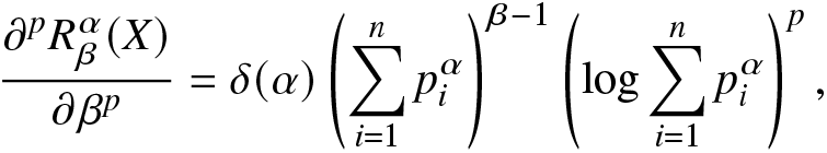
\end{eqnarray*} Further, the pth-order derivative of  $R_\beta^\alpha(X)$ with respect to β is obtained as
 \begin{align}
\frac{\partial^{p}R_\beta^\alpha(X)}{\partial \beta^p}=\delta(\alpha)\left(\sum_{i=1}^{n}p_i^\alpha\right)^{\beta-1}\left(\log\sum_{i=1}^{n}p_i^\alpha\right)^p,
\end{align}
\begin{align}
\frac{\partial^{p}R_\beta^\alpha(X)}{\partial \beta^p}=\delta(\alpha)\left(\sum_{i=1}^{n}p_i^\alpha\right)^{\beta-1}\left(\log\sum_{i=1}^{n}p_i^\alpha\right)^p,
\end{align}provided that the sum in (2.4) is convergent. In particular,
 \begin{align*}
\frac{\partial R_\beta^\alpha(X)}{\partial \beta}\Big|_{\beta=1}=\delta(\alpha)\log\sum_{i=1}^{n}p_i^\alpha
\end{align*}
\begin{align*}
\frac{\partial R_\beta^\alpha(X)}{\partial \beta}\Big|_{\beta=1}=\delta(\alpha)\log\sum_{i=1}^{n}p_i^\alpha
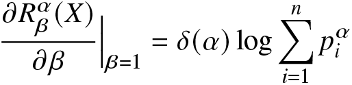
\end{align*}is the Rényi entropy of the discrete random variable X in Definition 2.1. Next, we obtain closed-form expressions of the Rényi entropy for some discrete distributions (see Table 1) using the proposed RIGF in (2.1). We mention here that the RIGF is a simple tool to obtain the Rényi entropy of probability distributions.
Table 1. The RIGF and Rényi entropy of some discrete distributions.
Next, we introduce the RIGF for a continuous random variable.
Definition 2.2. Let X be a continuous random variable with PDF  $f(\cdot)$. Then, for $0 \lt \alpha \lt \infty,~ \alpha\neq1,~ \beta \gt 0$, the RIGF of X is
 \begin{align}
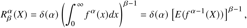
R^\alpha_\beta(X)=\delta(\alpha)\left(\int_{0}^{\infty}f^\alpha(x)dx\right)^{\beta-1}=\delta(\alpha)\left[E
(f^{\alpha-1}(X))\right]^{\beta-1},
\end{align}
\begin{align}
R^\alpha_\beta(X)=\delta(\alpha)\left(\int_{0}^{\infty}f^\alpha(x)dx\right)^{\beta-1}=\delta(\alpha)\left[E
(f^{\alpha-1}(X))\right]^{\beta-1},
\end{align} where  $\delta(\alpha)=\frac{1}{1-\alpha}$.
Note that the integral in (2.5) is convergent. The derivative of  $(2.5)$ with respect to β is
 \begin{align*}
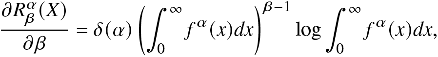
\frac{\partial R^\alpha_\beta(X)}{\partial\beta}=\delta(\alpha)\left(\int_{0}^{\infty}f^\alpha(x)dx\right)^{\beta-1}\log \int_{0}^{\infty}f^\alpha(x)dx,
\end{align*}
\begin{align*}
\frac{\partial R^\alpha_\beta(X)}{\partial\beta}=\delta(\alpha)\left(\int_{0}^{\infty}f^\alpha(x)dx\right)^{\beta-1}\log \int_{0}^{\infty}f^\alpha(x)dx,
\end{align*}and consequently, the pth-order derivative of RIGF, also known as the pth entropic moment, is obtained as
 \begin{align*}
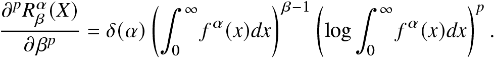
\frac{\partial^p R^\alpha_\beta(X)}{\partial\beta^p}=\delta(\alpha)\left(\int_{0}^{\infty}f^\alpha(x)dx\right)^{\beta-1}\left(\log \int_{0}^{\infty}f^\alpha(x)dx\right)^p.
\end{align*}
\begin{align*}
\frac{\partial^p R^\alpha_\beta(X)}{\partial\beta^p}=\delta(\alpha)\left(\int_{0}^{\infty}f^\alpha(x)dx\right)^{\beta-1}\left(\log \int_{0}^{\infty}f^\alpha(x)dx\right)^p.
\end{align*}We notice that the RIGF is convex with respect to β for α < 1 and concave for α > 1. Some important observations of the proposed RIGF are as follows:
• $R^\alpha_\beta(X)\big|_{\beta=1}=\delta(\alpha)$;
$\frac{\partial R^\alpha_\beta(X)}{\partial \beta}\Big|_{\beta=1}=H_{\alpha}(X)$, where
$H_{\alpha}(X)$ is as in (1.1);
$R^\alpha_\beta(X)\big|_{\beta=1}=\delta(\alpha)$;
$\frac{\partial R^\alpha_\beta(X)}{\partial \beta}\Big|_{\beta=1}=H_{\alpha}(X)$, where
$H_{\alpha}(X)$ is as in (1.1);•
$R^\alpha_\beta(X)\big|_{\beta=2, \alpha=2}=-IE(X)$, where IE(X) is the IE, given in (1.4).


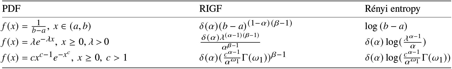
The expressions of the RIGF and Rényi entropy for some continuous distributions are presented in Table 2. Here,  $\Gamma(\cdot)$ denotes the complete gamma function. To observe the behavior of the RIGF of different distributions in Table 2 with respect to β, some graphical plots are presented in Figure 1. From these figures, we notice that they are increasing with respect to β for fixed α. Also, we observe from the graphs that the RIGF is concave when $\alpha=0.7 ( \lt 1)$ and convex when $\alpha=1.5 ( \gt 1).$
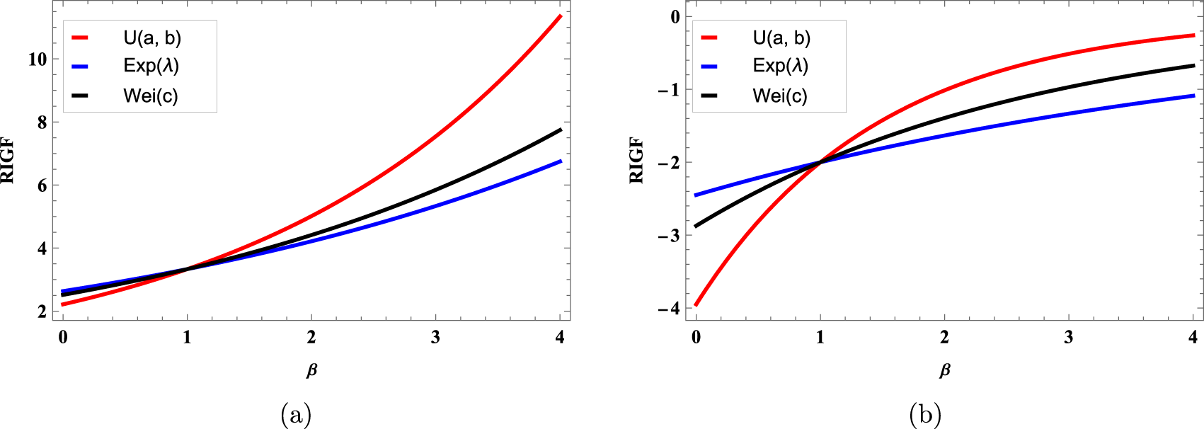
Figure 1. Plots of the RIGFs of uniform distribution ( $U(a,b)$) for $x\in[0.1,4]$, exponential distribution (Exp(λ)) for λ = 1.5, and Weibull (Wei(c)) distribution for $c=1.4,$ (a) for α = 0.7 and (b) for α = 1.5 in Table 2.
Table 2. The RIGF and Rényi entropy for uniform, exponential, and Weibull distributions. For convenience, we denote  $\omega_1=\frac{\alpha(c-1)+1}{c}.$
In the following proposition, we establish that the RIGF is shift independent, that is, it gives equal significance or weight to the occurrence of every event. We note that the shift-independent measures play a vital role in different fields, especially in information theory, pattern recognition, and signal processing. There is a chance of having time delays of signals in communication systems. In order to check the efficiency of such communication systems, the shift-independent measure is crucial since it allows to measure the information conveyed in these signals without requiring precise alignment. This procedure helps one to understand data transmission in different networks in a better way.
Proposition 2.3. Suppose the random variable X has PDF  $f(\cdot)$. Then, for a > 0 and $b\geq0$, the RIGF of $Y=aX+b$ is
 \begin{align}
R^\alpha_\beta(Y)=a^{(1-\alpha)(\beta-1)}R^\alpha_\beta(X),~~\alpha \gt 0,~~\alpha\ne 1,~~\beta \gt 0.
\end{align}
\begin{align}
R^\alpha_\beta(Y)=a^{(1-\alpha)(\beta-1)}R^\alpha_\beta(X),~~\alpha \gt 0,~~\alpha\ne 1,~~\beta \gt 0.
\end{align}Proof. Under the assumption made, the PDF of Y is obtained as  $g(x)=\frac{1}{a}f(\frac{x-b}{a}),$ where $x\ge b$. Now, using this PDF in Definition 2.2, the proof follows, and so it is omitted.
Remark 2.4. We note that some of the results presented here can be related to the properties of a variability measure in the sense of [Reference Bickel and Lehmann2]. For example, under suitable assumptions, the following properties hold:
• if X and Y are equal in law, then
$R^\alpha_\beta(X) = R^\alpha_\beta(Y)$;•
$R^\alpha_\beta(X) \gt 0$ for all β > 0 and
$0 \lt \alpha \lt 1;$•
$R^\alpha_\beta(X+b)=R^\alpha_\beta(X)$ for all
$b\ge 0$;•
$R^\alpha_\beta(a X)=aR^\alpha_\beta(X)$ for all a > 0, and α and β such that
$(1-\alpha)(\beta-1)=1$;•
$X\le_{disp}Y$ implies
$R^\alpha_\beta(X)\le R^\alpha_\beta(Y)$ (see Part (A) of Proposition 2.10).


In the information theory, it is always of interest to find a connection between a newly proposed information measure with other well-known information measures. In this regard, we next establish that the RIGF can be expressed in terms of the Shannon entropy of order q > 0. We recall that for a continuous random variable X, the Shannon entropy of order q is defined as (see [Reference Kharazmi and Balakrishnan18])
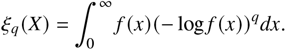 \begin{align}
\xi_{q}(X)=\int_{0}^{\infty}f(x)(-\log f(x))^qdx.
\end{align}
\begin{align}
\xi_{q}(X)=\int_{0}^{\infty}f(x)(-\log f(x))^qdx.
\end{align}Proposition 2.5. Let  $f(\cdot)$ be the PDF of a random variable X. Then, for $\beta\geq0$ and $0 \lt \alpha \lt \infty, ~\alpha\neq1$, the RIGF of X can be represented as
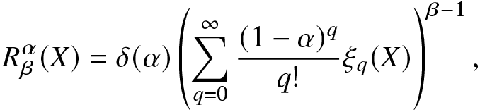 \begin{align}
R^\alpha_\beta(X)=\delta(\alpha)\left(\sum_{q=0}^{\infty}\frac{(1-\alpha)^{q}}{q!}\xi_q(X)\right)^{\beta-1},
\end{align}
\begin{align}
R^\alpha_\beta(X)=\delta(\alpha)\left(\sum_{q=0}^{\infty}\frac{(1-\alpha)^{q}}{q!}\xi_q(X)\right)^{\beta-1},
\end{align} where  $\xi_q(X)$ is as given in (2.7).
Proof. From (2.5), we have
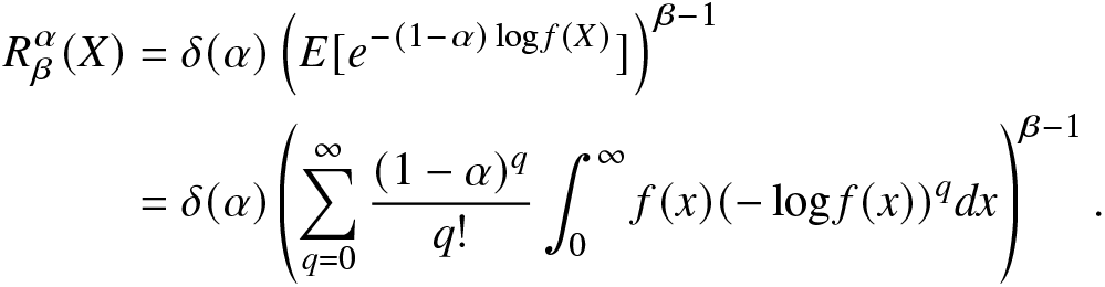 \begin{align}
R^\alpha_\beta(X)
&=\delta(\alpha)\left(E[e^{-(1-\alpha)\log f(X)}]\right)^{\beta-1}\nonumber\\
&=\delta(\alpha)\left(\sum_{q=0}^{\infty}\frac{(1-\alpha)^q}{q!}\int_{0}^{\infty}f(x)(-\log f(x))^qdx\right)^{\beta-1}.
\end{align}
\begin{align}
R^\alpha_\beta(X)
&=\delta(\alpha)\left(E[e^{-(1-\alpha)\log f(X)}]\right)^{\beta-1}\nonumber\\
&=\delta(\alpha)\left(\sum_{q=0}^{\infty}\frac{(1-\alpha)^q}{q!}\int_{0}^{\infty}f(x)(-\log f(x))^qdx\right)^{\beta-1}.
\end{align}From (2.9), the result in (2.8) follows directly, which completes the proof of the proposition.
We now obtain upper and lower bounds for the RIGF. We recall that the bounds are useful to treat them as estimates when the actual form of the RIGF for distributions is difficult to derive.
Proposition 2.6. Suppose X is a continuous random variable with PDF  $f(\cdot)$. Then,
(A) for
$0 \lt \alpha \lt 1$, we have
(2.10)\begin{equation}
R^\alpha_\beta(X)\left\{
\begin{array}{ll}
\leq \delta(\alpha)G_{\alpha\beta-\alpha-\beta+2}(X),~
if~~0 \lt \beta \lt 1\ and\ \beta\geq2,
\\
\geq\frac{1}{2}R^{\frac{\alpha+1}{2}}_{2\beta-1}(X),~~~~~~~~~~~if~ \beta\geq1,
\\
\leq\frac{1}{2}R^{\frac{\alpha+1}{2}}_{2\beta-1}(X),~~~~~~~~~~~if~ 0 \lt \beta \lt 1;
\end{array}
\right.
\end{equation}(B) for α > 1, we have
(2.11)\begin{equation}
R^\alpha_\beta(X)\left\{
\begin{array}{ll}
\leq \delta(\alpha)G_{\alpha\beta-\alpha-\beta+2}(X),~
if~~1 \lt \beta \lt 2,
\\
\leq\frac{1}{2}R^{\frac{\alpha+1}{2}}_{2\beta-1}(X),~~~~~~~~~~if~ \beta\geq1,
\\
\geq\frac{1}{2}R^{\frac{\alpha+1}{2}}_{2\beta-1}(X),~~~~~~~~~~if~ 0 \lt \beta \lt 1,
\end{array}
\right.
\end{equation}


where  $G_{\alpha\beta-\alpha-\beta+2}(X)=\int_{0}^{\infty}f^{\alpha\beta-\alpha-\beta+2}(x)dx$ is the IGF of X.
Proof. (A) Let  $\alpha\in(0,1)$. Consider a positive real-valued function $g(\cdot)$ such that $\int_{0}^{\infty}g(x)dx=1$. Then, the generalized Jensen inequality for a convex function $\psi(\cdot)$ is given by
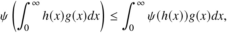 \begin{align}
\psi\left(\int_{0}^{\infty}h(x)g(x)dx\right)\leq\int_{0}^{\infty}\psi(h(x))g(x)dx,
\end{align}
\begin{align}
\psi\left(\int_{0}^{\infty}h(x)g(x)dx\right)\leq\int_{0}^{\infty}\psi(h(x))g(x)dx,
\end{align} where  $h(\cdot)$ is a real-valued function. Set $g(x)=f(x)$, $\psi(x)=x^{\beta-1}$ and $h(x)=f^{\alpha-1}(x)$. For $0 \lt \beta \lt 1$ and $\beta\geq2$, the function $\psi(x)$ is convex with respect to x. Thus, from (2.12), we have
 \begin{align}
&\delta(\alpha)\left(\int_{0}^{\infty}f^\alpha(x)dx\right)^{\beta-1}\leq \delta(\alpha)\int_{0}^{\infty}f^{\alpha\beta-\alpha-\beta+2}(x)dx
\Rightarrow R^\alpha_\beta(X)\leq \delta(\alpha)G_{\alpha\beta-\alpha-\beta+2}(X),
\end{align}
\begin{align}
&\delta(\alpha)\left(\int_{0}^{\infty}f^\alpha(x)dx\right)^{\beta-1}\leq \delta(\alpha)\int_{0}^{\infty}f^{\alpha\beta-\alpha-\beta+2}(x)dx
\Rightarrow R^\alpha_\beta(X)\leq \delta(\alpha)G_{\alpha\beta-\alpha-\beta+2}(X),
\end{align}which establishes the first inequality in (2.10).
In order to establish the second and third inequalities in (2.10), we require the Cauchy–Schwartz inequality. It is well-known that, for two real integrable functions  $h_1(x)$ and $h_2(x)$, the Cauchy–Schwartz inequality is given by
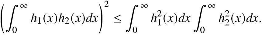 \begin{align}
\left(\int_{0}^{\infty}h_1(x)h_2(x)dx\right)^2\leq \int_{0}^{\infty}h^2_1(x)dx\int_{0}^{\infty}h^2_2(x)dx.
\end{align}
\begin{align}
\left(\int_{0}^{\infty}h_1(x)h_2(x)dx\right)^2\leq \int_{0}^{\infty}h^2_1(x)dx\int_{0}^{\infty}h^2_2(x)dx.
\end{align} Taking  $h_1(x)=f^{\frac{\alpha}{2}}(x)$ and $h_2(x)=f^{\frac{1}{2}}(x)$ in (2.14), we obtain
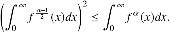 \begin{align}
&\left(\int_{0}^{\infty}f^{\frac{\alpha+1}{2}}(x)dx\right)^2\leq \int_{0}^{\infty}f^\alpha(x)dx.
\end{align}
\begin{align}
&\left(\int_{0}^{\infty}f^{\frac{\alpha+1}{2}}(x)dx\right)^2\leq \int_{0}^{\infty}f^\alpha(x)dx.
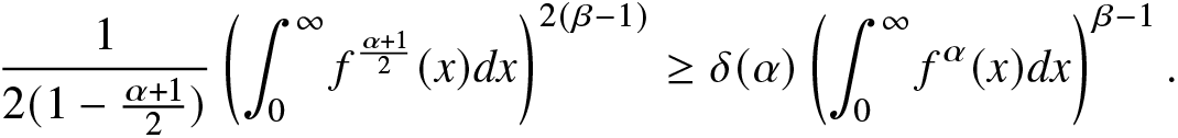
\end{align} Now, from (2.15), we have for  $\beta\geq1$,
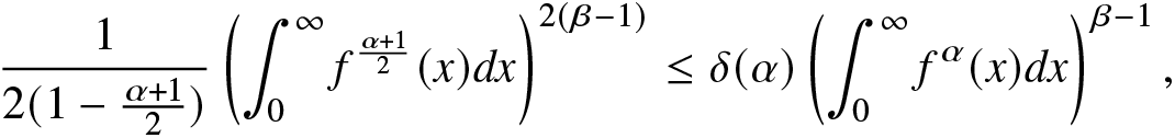 \begin{align}
\frac{1}{2(1-\frac{\alpha+1}{2})}\left(\int_{0}^{\infty}f^{\frac{\alpha+1}{2}}(x)dx\right)^{2(\beta-1)}\leq \delta(\alpha)\left(\int_{0}^{\infty}f^\alpha(x)dx\right)^{\beta-1},
\end{align}
\begin{align}
\frac{1}{2(1-\frac{\alpha+1}{2})}\left(\int_{0}^{\infty}f^{\frac{\alpha+1}{2}}(x)dx\right)^{2(\beta-1)}\leq \delta(\alpha)\left(\int_{0}^{\infty}f^\alpha(x)dx\right)^{\beta-1},
\end{align} and for  $0 \lt \beta \lt 1$,
 \begin{align}
\frac{1}{2(1-\frac{\alpha+1}{2})}\left(\int_{0}^{\infty}f^{\frac{\alpha+1}{2}}(x)dx\right)^{2(\beta-1)}\geq \delta(\alpha)\left(\int_{0}^{\infty}f^\alpha(x)dx\right)^{\beta-1}.
\end{align}
\begin{align}
\frac{1}{2(1-\frac{\alpha+1}{2})}\left(\int_{0}^{\infty}f^{\frac{\alpha+1}{2}}(x)dx\right)^{2(\beta-1)}\geq \delta(\alpha)\left(\int_{0}^{\infty}f^\alpha(x)dx\right)^{\beta-1}.
\end{align}The second and third inequalities in (2.10) now follow from (2.16) and (2.17), respectively.
The proof of Part (B) for α > 1 is similar to the proof of Part (A) for different values of β. So, the proof is omitted for brevity.
We now present an example to validate the result in Proposition 2.6.
Example 2.7. Suppose X has an exponential distribution with PDF  $f(x)=\lambda e^{-\lambda x},~ x\ge 0,~\lambda \gt 0$. Then,
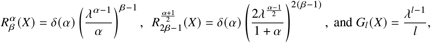 \begin{align*}
R^\alpha_\beta(X)=\delta(\alpha)\left(\frac{\lambda^{\alpha-1}}{\alpha}\right)^{\beta-1},~~
R^{\frac{\alpha+1}{2}}_{2\beta-1}(X)=\delta(\alpha)\left(\frac{2\lambda^{\frac{\alpha-1}{2}}}{1+\alpha}\right)^{2(\beta-1)},~\text{and}~
G_{l}(X)=\frac{\lambda^{l-1}}{l},
\end{align*}
\begin{align*}
R^\alpha_\beta(X)=\delta(\alpha)\left(\frac{\lambda^{\alpha-1}}{\alpha}\right)^{\beta-1},~~
R^{\frac{\alpha+1}{2}}_{2\beta-1}(X)=\delta(\alpha)\left(\frac{2\lambda^{\frac{\alpha-1}{2}}}{1+\alpha}\right)^{2(\beta-1)},~\text{and}~
G_{l}(X)=\frac{\lambda^{l-1}}{l},
\end{align*} where  $l=\alpha\beta-\alpha-\beta+2.$ In order to check the first two inequalities in (2.11), we have plotted the graphs of $R^\alpha_\beta(X)$, $\frac{1}{2}R^{\frac{\alpha+1}{2}}_{2\beta-1}(X)$ and $\delta(\alpha)G_{l}(X)$ in Figure 2 for some choices of λ, $\beta,$ and α.
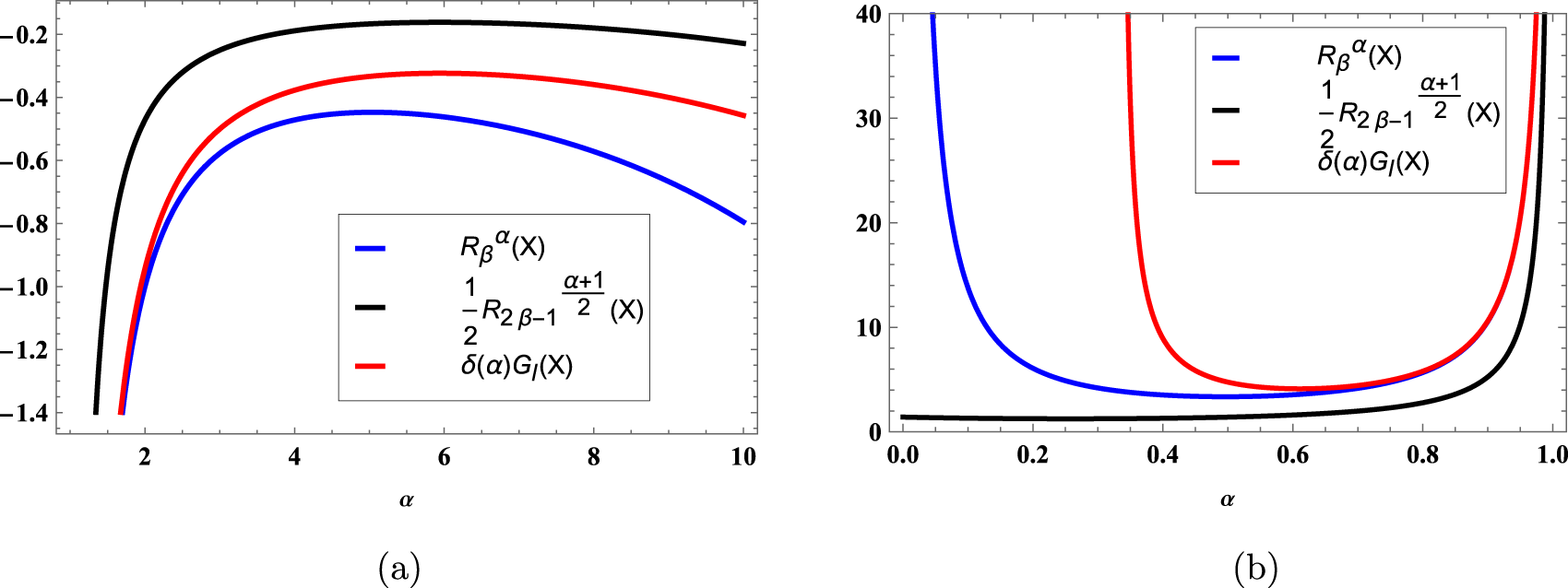
Figure 2. Graphs of  $R^\alpha_\beta(X)$, $\frac{1}{2}R^{\frac{\alpha+1}{2}}_{2\beta-1}(X)$ and $\delta(\alpha)G_{l}(X),$ for (a) $\lambda=2,~\beta=1.5$, and α > 1 and (b) $\lambda=2,~\beta=2.5$ and α < 1 in Example 2.7.
Suppose X and Y have PDFs  $f(\cdot)$ and $g(\cdot)$, respectively. The PDF of the sum of X and Y, say $Z=X+Y$, is
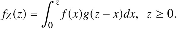 \begin{align*}
f_{Z}(z)=\int_{0}^{z}f(x)g(z-x)dx,~~z\ge 0.
\end{align*}
\begin{align*}
f_{Z}(z)=\int_{0}^{z}f(x)g(z-x)dx,~~z\ge 0.
\end{align*}This is known as the convolution of X and Y. The convolution property is essential in various fields, particularly in signal processing, image processing, and deep learning. Convolution is used to filter signals, extract features, and perform operations like smoothing and differentiation in signal processing. In image processing, it is fundamental in operations like blurring, sharpening, and edge detection. Here, we study the RIGF for the convolution of two random variables X and Y.
Proposition 2.8. Let  $f(\cdot)$ and $g(\cdot)$ be the PDFs of independent random variables X and Y, respectively. Further, let $Z=X+Y.$ Then, for $0 \lt \alpha \lt \infty$, α ≠ 1,
(A)
$R^\alpha_\beta(Z)\leq R^\alpha_\beta(X)(G_\alpha(Y))^{\beta-1}$, if
$0 \lt \beta \lt 1$;(B)
$R^\alpha_\beta(Z)\geq R^\alpha_\beta(X)(G_\alpha(Y))^{\beta-1}$, if
$\beta\geq1$,


where  $G_\alpha(Y)$ is the IGF of Y.
Proof. (A) Case I: Consider  $0 \lt \beta \lt 1$ and $0 \lt \alpha \lt 1$. From (2.5), applying Jensen’s inequality and Fubuni’s theorem, we obtain
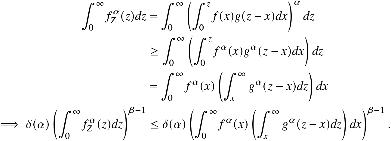 \begin{align}
\int_{0}^{\infty}f^\alpha_Z(z)dz&=\int_{0}^{\infty}\left(\int_{0}^{z}f(x)g(z-x)dx\right)^\alpha dz\nonumber\\
&\geq \int_{0}^{\infty}\left(\int_{0}^{z}f^\alpha(x)g^\alpha(z-x)dx\right)dz\nonumber\\
&=\int_{0}^{\infty}f^\alpha(x)\left(\int_{x}^{\infty}g^\alpha(z-x)dz\right)dx\nonumber\\
\implies\delta(\alpha)\left(\int_{0}^{\infty}f^\alpha_Z(z)dz\right)^{\beta-1}&\leq\delta(\alpha)\left(\int_{0}^{\infty}f^\alpha(x)\left(\int_{x}^{\infty}g^\alpha(z-x)dz\right)dx\right)^{\beta-1}.
\end{align}
\begin{align}
\int_{0}^{\infty}f^\alpha_Z(z)dz&=\int_{0}^{\infty}\left(\int_{0}^{z}f(x)g(z-x)dx\right)^\alpha dz\nonumber\\
&\geq \int_{0}^{\infty}\left(\int_{0}^{z}f^\alpha(x)g^\alpha(z-x)dx\right)dz\nonumber\\
&=\int_{0}^{\infty}f^\alpha(x)\left(\int_{x}^{\infty}g^\alpha(z-x)dz\right)dx\nonumber\\
\implies\delta(\alpha)\left(\int_{0}^{\infty}f^\alpha_Z(z)dz\right)^{\beta-1}&\leq\delta(\alpha)\left(\int_{0}^{\infty}f^\alpha(x)\left(\int_{x}^{\infty}g^\alpha(z-x)dz\right)dx\right)^{\beta-1}.
\end{align} Case II: Consider  $0 \lt \beta \lt 1$ and α > 1. Here, the proof follows similarly to the Case I. Thus, the result in Part (A) is proved.
The proof of Part (B) is similar to that of Part (A) and is therefore omitted.
The following corollary is immediate from Proposition 2.8.
Corollary 2.9. For independent and identically distributed random variables X and Y, with  $0 \lt \alpha \lt \infty$, α ≠ 1, we have
(A)
$R^\alpha_\beta(Z)\leq R^\alpha_{2\beta-1}(X)$, if
$0 \lt \beta \lt 1$,(B)
$R^\alpha_\beta(Z)\geq R^\alpha_{2\beta-1}(X)$, if
$\beta\geq1$.


Numerous fields have benefited from the usefulness of the concept of stochastic orderings, including actuarial science, survival analysis, finance, risk theory, nonparametric approaches, and reliability theory. Suppose X and Y are two random variables with corresponding PDFs  $f(\cdot)$ and $g(\cdot)$ and CDFs $F(\cdot)$ and $G(\cdot)$, respectively. Then, X is less dispersed than Y, denoted by $X\leq_{disp}Y$, if $g(G^{-1}(x))\leq f(F^{-1}(x))$, for all $x\in(0,1)$. Further, X is said to be smaller than Y in the sense of the usual stochastic order (denote by $X\le_{st}Y$) if $F(x)\ge G(x)$, for x > 0. For more details, one may refer to [Reference Shaked and Shanthikumar39].
The quantile representation of the RIGF of X is given by
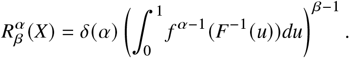 \begin{eqnarray*}
R^{\alpha}_{\beta}(X)=\delta(\alpha)\left(\int_{0}^{1}f^{\alpha-1}(F^{-1}(u))du\right)^{{\beta-1}}.
\end{eqnarray*}
\begin{eqnarray*}
R^{\alpha}_{\beta}(X)=\delta(\alpha)\left(\int_{0}^{1}f^{\alpha-1}(F^{-1}(u))du\right)^{{\beta-1}}.
\end{eqnarray*}The next proposition deals with the comparisons of RIGFs of two random variables. The sufficient conditions here depend on the dispersive order and some restrictions of the parameters.
Proposition 2.10. Consider two random variables X and Y such that  $X\leq_{disp}Y$. Then, we have
(A)
$R^{\alpha}_{\beta}(X)\leq R^{\alpha}_{\beta}(Y)$; for
$\{\alpha \lt 1;\beta\geq1\}$ or
$\{\alpha \gt 1; \beta\ge1\},$(B)
$R^{\alpha}_{\beta}(X)\geq R^{\alpha}_{\beta}(Y)$, for
$\{\alpha \lt 1;\beta \lt 1\}$ or
$\{\alpha \gt 1; \beta \lt 1\}$.


Proof. (A) Consider the case  $\{\alpha \lt 1;\beta\geq1\}$. The proof for the case $\{\alpha \gt 1; \beta\ge1\}$ is quite similar. Under the assumption made, we have
 \begin{align}
X\leq_{disp}Y\implies f(F^{-1}(u))\geq g(G^{-1}(u))\implies f^{\alpha-1}(F^{-1}(u))\leq g^{\alpha-1}(G^{-1}(u))
\end{align}
\begin{align}
X\leq_{disp}Y\implies f(F^{-1}(u))\geq g(G^{-1}(u))\implies f^{\alpha-1}(F^{-1}(u))\leq g^{\alpha-1}(G^{-1}(u))
\end{align} for all  $u\in(0,1).$ Thus, from (2.19), we have
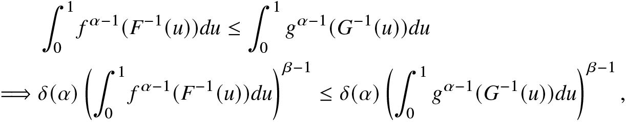 \begin{align*}
&\int_{0}^{1}f^{\alpha-1}(F^{-1}(u))du\leq\int_{0}^{1}g^{\alpha-1}(G^{-1}(u))du\nonumber\\
\implies&\delta(\alpha)\left(\int_{0}^{1}f^{\alpha-1}(F^{-1}(u))du\right)^{\beta-1}\leq \delta(\alpha)\left(\int_{0}^{1}g^{\alpha-1}(G^{-1}(u))du\right)^{\beta-1},
\end{align*}
\begin{align*}
&\int_{0}^{1}f^{\alpha-1}(F^{-1}(u))du\leq\int_{0}^{1}g^{\alpha-1}(G^{-1}(u))du\nonumber\\
\implies&\delta(\alpha)\left(\int_{0}^{1}f^{\alpha-1}(F^{-1}(u))du\right)^{\beta-1}\leq \delta(\alpha)\left(\int_{0}^{1}g^{\alpha-1}(G^{-1}(u))du\right)^{\beta-1},
\end{align*}establishing the required result. The proof for Part (B) is similar and is therefore omitted.
Let X be a random variable with CDF  $F(\cdot)$ and quantile function $Q_{X}(u)$, for $0 \lt u \lt 1,$ given by
 \begin{eqnarray*}
Q_{X}(u)=F^{-1}(u)=\inf\{x:F(x)\ge u\},~u\in(0,1).
\end{eqnarray*}
\begin{eqnarray*}
Q_{X}(u)=F^{-1}(u)=\inf\{x:F(x)\ge u\},~u\in(0,1).
\end{eqnarray*} It is well-known that  $X\le_{st} Y \Longleftrightarrow Q_{X}(u)\le Q_{Y}(u),~u\in(0,1),$ where $Q_{Y}(\cdot)$ is the quantile function of $Y.$ Moreover, we know that if X and Y are such that they have a common finite left end point of their supports, then $X\le_{disp}Y\Rightarrow X\le_{st} Y$ (see [Reference Shaked and Shanthikumar39]). Next, we consider a convex and increasing function $\psi(\cdot)$ and then obtain inequalities between the RIGFs of $\psi(X)$ and $\psi(Y).$
Proposition 2.11. For the random variables X and Y, with  $X\le_{disp}Y,$ let $\psi(\cdot)$ be convex and strictly increasing. Then, we have
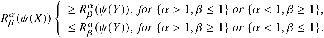 \begin{equation}
R^\alpha_\beta(\psi(X))\left\{
\begin{array}{ll}
\ge R^\alpha_\beta(\psi(Y)),~
for~\{\alpha \gt 1,\beta\le1\}~or~\{\alpha \lt 1,\beta\ge1\},
\\
\le R^\alpha_\beta(\psi(Y)),~for~\{\alpha \gt 1,\beta\ge1\}~or~\{\alpha \lt 1,\beta\le1\}.
\end{array}
\right.
\end{equation}
\begin{equation}
R^\alpha_\beta(\psi(X))\left\{
\begin{array}{ll}
\ge R^\alpha_\beta(\psi(Y)),~
for~\{\alpha \gt 1,\beta\le1\}~or~\{\alpha \lt 1,\beta\ge1\},
\\
\le R^\alpha_\beta(\psi(Y)),~for~\{\alpha \gt 1,\beta\ge1\}~or~\{\alpha \lt 1,\beta\le1\}.
\end{array}
\right.
\end{equation}Proof. Using the PDF of  $\psi(X)$, the RIGF of $\psi(X)$ can be expressed as
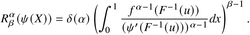 \begin{eqnarray*}
R_{\beta}^{\alpha}(\psi(X))=\delta(\alpha)\left(\int_{0}^{1}\frac{f^{\alpha-1}(F^{-1}(u))}{(\psi^{\prime}(F^{-1}(u)))^{\alpha-1}}dx\right)^{\beta-1}.
\end{eqnarray*}
\begin{eqnarray*}
R_{\beta}^{\alpha}(\psi(X))=\delta(\alpha)\left(\int_{0}^{1}\frac{f^{\alpha-1}(F^{-1}(u))}{(\psi^{\prime}(F^{-1}(u)))^{\alpha-1}}dx\right)^{\beta-1}.
\end{eqnarray*} Since  $\psi(\cdot)$ is assumed to be convex and increasing, with the assumption that $X\le_{disp}Y$, we obtain
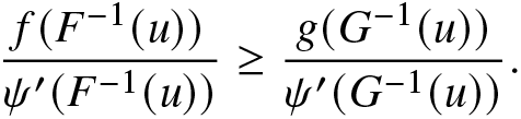 \begin{eqnarray*}
\frac{f(F^{-1}(u))}{\psi'(F^{-1}(u))}\ge \frac{g(G^{-1}(u))}{\psi'(G^{-1}(u))}.
\end{eqnarray*}
\begin{eqnarray*}
\frac{f(F^{-1}(u))}{\psi'(F^{-1}(u))}\ge \frac{g(G^{-1}(u))}{\psi'(G^{-1}(u))}.
\end{eqnarray*} Now, using α > 1 and  $\beta\le1,$ the first inequality in (2.20) follows easily. The inequalities for other restrictions on α and β can be established similarly. This completes the proof of the proposition.
Escort distributions are useful in modeling and analyzing complex systems, where traditional probabilistic models fail. They provide a flexible and robust framework for dealing with non-standard distributions, making them essential in many areas of research and applications. Escort distributions are also used for the characteristic of chaos and multifractals in statistical physics. Abe [Reference Abe1] showed quantitatively that it is inappropriate to use the original distribution instead of the escort distribution for calculating the expectation values of physical quantities in nonextensive statistical mechanics. Suppose X and Y are two continuous random variables and their PDFs are  $f(\cdot)$ and $g(\cdot)$, respectively. Then, the PDFs of the escort and generalized escort distributions are, respectively, given by
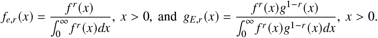 \begin{align}
f_{e,r}(x)=\frac{f^r(x)}{\int_{0}^{\infty}f^r(x)dx},~ x \gt 0,~\mbox{and}~~g_{E,r}(x)=\frac{f^r(x)g^{1-r}(x)}{\int_{0}^{\infty}f^r(x)g^{1-r}(x)dx},~x \gt 0.
\end{align}
\begin{align}
f_{e,r}(x)=\frac{f^r(x)}{\int_{0}^{\infty}f^r(x)dx},~ x \gt 0,~\mbox{and}~~g_{E,r}(x)=\frac{f^r(x)g^{1-r}(x)}{\int_{0}^{\infty}f^r(x)g^{1-r}(x)dx},~x \gt 0.
\end{align}In the following proposition, we express the RIGF of the escort distribution in terms of the RIGF of baseline distribution. The result follows directly from (2.5) and (2.21).
Proposition 2.12. Let X be a continuous random variable with PDF  $f(\cdot)$. Then, the RIGF of the escort random variable of order r can be obtained as
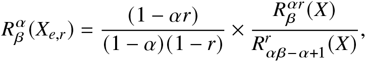 \begin{align*}
R^\alpha_\beta(X_{e,r})=\frac{(1-\alpha r)}{(1-\alpha)(1-r)}\times \frac{R^{\alpha r}_\beta(X)}{R^r_{\alpha\beta-\alpha+1}(X)},
\end{align*}
\begin{align*}
R^\alpha_\beta(X_{e,r})=\frac{(1-\alpha r)}{(1-\alpha)(1-r)}\times \frac{R^{\alpha r}_\beta(X)}{R^r_{\alpha\beta-\alpha+1}(X)},
\end{align*} where  $X_{e,r}$ is the escort random variable.
3. Rényi divergence information generating function
We propose an IGF of the Rényi divergence. Suppose X and Y are two continuous random variables and their PDFs are  $f(\cdot)$ and $g(\cdot),$ respectively. Then, the RDIGF is given by
 \begin{align}
RD^\alpha_\beta(X,Y)=\delta^*(\alpha)\left(\int_{0}^{\infty}\left(\frac{f(x)}{g(x)}\right)^\alpha g(x)dx\right)^{\beta-1}=\delta^*(\alpha)\left(E_g\bigg[\frac{f(X)}{g(X)}\bigg]^\alpha\right)^{\beta-1}.
\end{align}
\begin{align}
RD^\alpha_\beta(X,Y)=\delta^*(\alpha)\left(\int_{0}^{\infty}\left(\frac{f(x)}{g(x)}\right)^\alpha g(x)dx\right)^{\beta-1}=\delta^*(\alpha)\left(E_g\bigg[\frac{f(X)}{g(X)}\bigg]^\alpha\right)^{\beta-1}.
\end{align} Clearly, the integral in (3.1) exists for  $0 \lt \alpha \lt \infty$ and β > 0. The kth-order derivative of (3.1) with respect to β is obtained as
 \begin{align}
\frac{\partial RD^\alpha_\beta(X,Y)}{\partial \beta^k}=\delta^*(\alpha)\left(\int_{0}^{\infty}\left(\frac{f(x)}{g(x)}\right)^\alpha g(x)dx\right)^{\beta-1}\left(\log\int_{0}^{\infty}\left(\frac{f(x)}{g(x)}\right)^\alpha g(x)dx\right)^k,
\end{align}
\begin{align}
\frac{\partial RD^\alpha_\beta(X,Y)}{\partial \beta^k}=\delta^*(\alpha)\left(\int_{0}^{\infty}\left(\frac{f(x)}{g(x)}\right)^\alpha g(x)dx\right)^{\beta-1}\left(\log\int_{0}^{\infty}\left(\frac{f(x)}{g(x)}\right)^\alpha g(x)dx\right)^k,
\end{align}provided the integral exists. The following observations from (3.1) and (3.2) can be readily made:
•
$RD^\alpha_\beta(X,Y)|_{\beta=1}=\delta^*(\alpha)$;
$\frac{\partial}{\partial \beta}RD^\alpha_\beta(X,Y)|_{\beta=1}=RD(X,Y)$;•
$RD^\alpha_\beta(X,Y)=\alpha \delta^*(\alpha)RD^{1-\alpha}_\beta(Y,X)$,


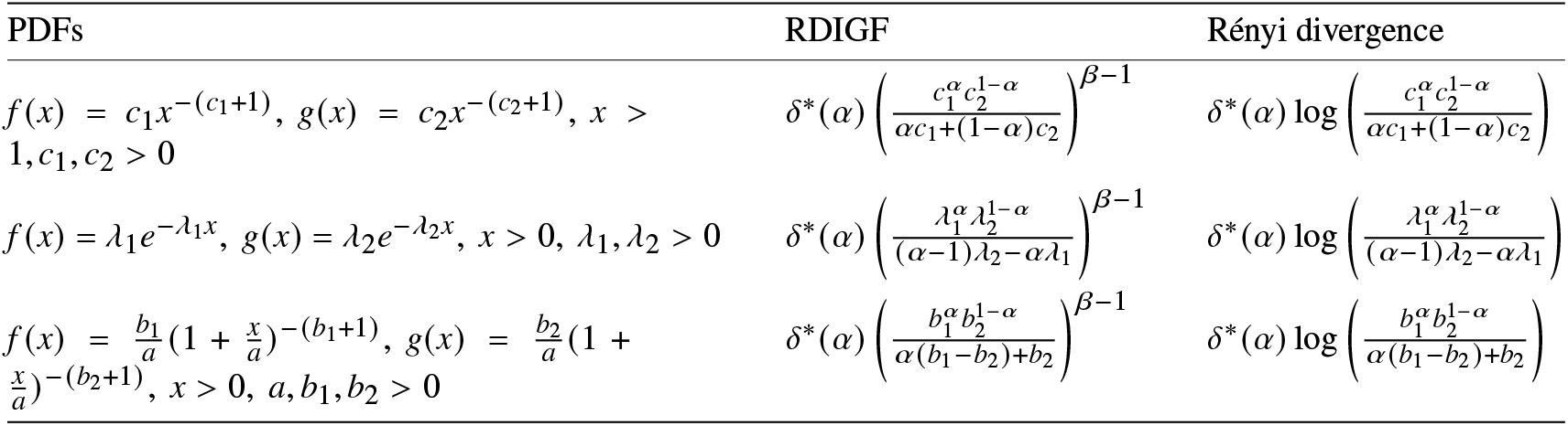
where  $RD(X,Y)$ is the Rényi divergence between X and Y given in (1.1). In Table 3, we present closed-form expressions of the RDIGF and Rényi divergence for some continuous distributions. In addition, to check the behavior of the RDIGFs in Table 3, we plot them in Figure 3. We notice that the RDIGFs are increasing with respect to β > 0.
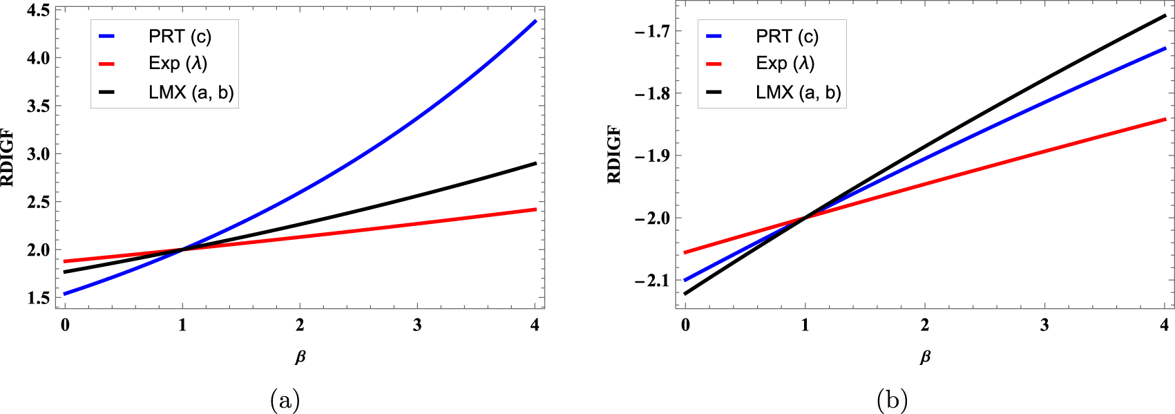
Figure 3. Plots of the RDIGFs of Pareto type-I (PRT) with  $c_1=0.8,~c_2=1.5$, exponential (Exp) with $\lambda_1=0.8,~\lambda_2=0.5,$ and Lomax (LMX) distributions with $a=0.5,~b_1=0.8,$ and $b_2=0.4$ when (a) α = 0.5 and (b) α = 1.5.
Table 3. The RDIGF and Rényi divergence for Pareto type-I, exponential, and Lomax distributions.
The following proposition states that the RDIGF between two random variables X and Y becomes the RIGF of X if Y follows uniform distribution in  $[0,1]$. The proof here is omitted since it is straightforward.
Proposition 3.1. Let X be a continuous random variable and Y be a uniform random variable, i.e.  $Y\sim U(0,1)$. Then, the RDIGF of X reduces to the RIGF of X.
Next, we establish a relation between the RIGF and RDIGF. In this regard, we consider the generalized escort distribution with PDF as in (2.21).
Proposition 3.2. Let  $Y_{e,r}$, $X_{e,r}$ be the escort random variables and $Y_{E,r}$ be the generalized escort random variable. Then,
 \begin{align*}
R^\alpha_\beta(Y_{E,r})RD^r_{\alpha\beta-\alpha+1}(X,Y)=(1-\alpha)R^\alpha_{r\beta-r+1}(X)R^\alpha_{(1-r)(\beta-1)+1}(Y)RD^r_\beta(X_{e,\alpha},Y_{e,\alpha}).
\end{align*}
\begin{align*}
R^\alpha_\beta(Y_{E,r})RD^r_{\alpha\beta-\alpha+1}(X,Y)=(1-\alpha)R^\alpha_{r\beta-r+1}(X)R^\alpha_{(1-r)(\beta-1)+1}(Y)RD^r_\beta(X_{e,\alpha},Y_{e,\alpha}).
\end{align*}Proof. Using (2.5) and (2.21), we obtain
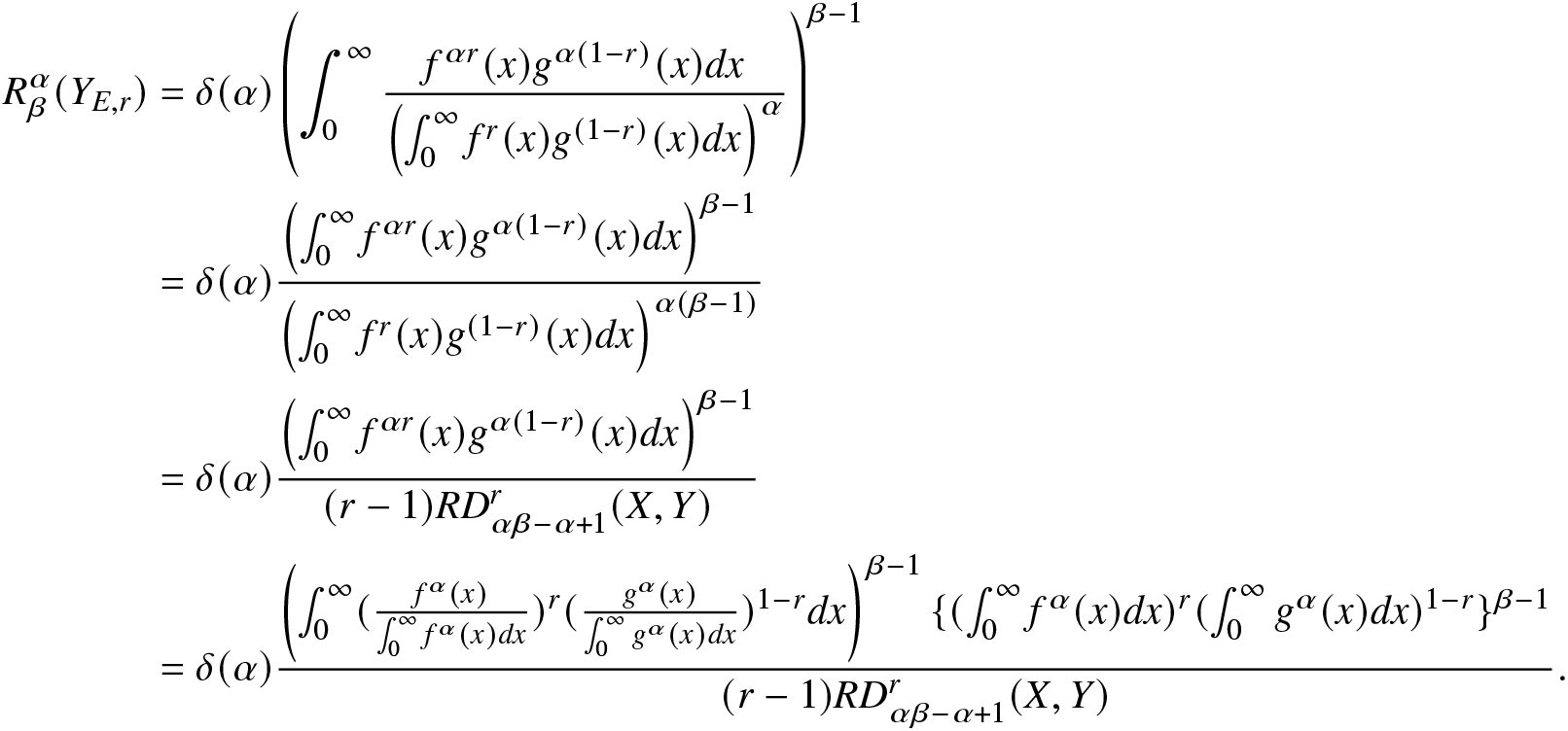 \begin{align}
R^\alpha_\beta(Y_{E,r})&=\delta(\alpha)\left(\int_{0}^{\infty}\frac{f^{\alpha r}(x)g^{\alpha(1-r)}(x)dx}{\left(\int_{0}^{\infty}f^r(x)g^{(1-r)}(x)dx\right)^\alpha}\right)^{\beta-1}\nonumber\\
&=\delta(\alpha)\frac{\left(\int_{0}^{\infty}f^{\alpha r}(x)g^{\alpha(1-r)}(x)dx\right)^{\beta-1}}{\left(\int_{0}^{\infty}f^r(x)g^{(1-r)}(x)dx\right)^{\alpha(\beta-1)}}\nonumber\\
&=\delta(\alpha)\frac{\left(\int_{0}^{\infty}f^{\alpha r}(x)g^{\alpha(1-r)}(x)dx\right)^{\beta-1}}{(r-1)RD^r_{\alpha\beta-\alpha+1}(X,Y)}\nonumber\\
&=\delta(\alpha)\frac{\left(\int_{0}^{\infty}(\frac{f^{\alpha}(x)}{\int_{0}^{\infty}f^{\alpha}(x)dx})^r(\frac{g^{\alpha}(x)}{\int_{0}^{\infty}g^{\alpha}(x)dx})^{1-r}dx\right)^{\beta-1}\{(\int_{0}^{\infty}f^{\alpha}(x)dx)^{r}(\int_{0}^{\infty}g^{\alpha}(x)dx)^{1-r}\}^{\beta-1}}{(r-1)RD^r_{\alpha\beta-\alpha+1}(X,Y)}.
\end{align}
\begin{align}
R^\alpha_\beta(Y_{E,r})&=\delta(\alpha)\left(\int_{0}^{\infty}\frac{f^{\alpha r}(x)g^{\alpha(1-r)}(x)dx}{\left(\int_{0}^{\infty}f^r(x)g^{(1-r)}(x)dx\right)^\alpha}\right)^{\beta-1}\nonumber\\
&=\delta(\alpha)\frac{\left(\int_{0}^{\infty}f^{\alpha r}(x)g^{\alpha(1-r)}(x)dx\right)^{\beta-1}}{\left(\int_{0}^{\infty}f^r(x)g^{(1-r)}(x)dx\right)^{\alpha(\beta-1)}}\nonumber\\
&=\delta(\alpha)\frac{\left(\int_{0}^{\infty}f^{\alpha r}(x)g^{\alpha(1-r)}(x)dx\right)^{\beta-1}}{(r-1)RD^r_{\alpha\beta-\alpha+1}(X,Y)}\nonumber\\
&=\delta(\alpha)\frac{\left(\int_{0}^{\infty}(\frac{f^{\alpha}(x)}{\int_{0}^{\infty}f^{\alpha}(x)dx})^r(\frac{g^{\alpha}(x)}{\int_{0}^{\infty}g^{\alpha}(x)dx})^{1-r}dx\right)^{\beta-1}\{(\int_{0}^{\infty}f^{\alpha}(x)dx)^{r}(\int_{0}^{\infty}g^{\alpha}(x)dx)^{1-r}\}^{\beta-1}}{(r-1)RD^r_{\alpha\beta-\alpha+1}(X,Y)}.
\end{align}Now, the required result follows easily from (3.3).
Monotone functions are fundamental in many theoretical and practical applications due to their predictability, order-preserving nature, and the mathematical simplicity they bring to various problems. In optimization problems, monotone functions are particularly useful because they simplify the process of finding maximum or minimum values. In statistics, monotone likelihood ratios are used in hypothesis testing and decision theory, where the monotonicity of certain functions ensures the validity of statistical tests and models. In the following, we discuss the effect of the RDIGF for monotone transformations.
Proposition 3.3. Suppose  $f(\cdot)$ and $g(\cdot)$ are the PDFs of X and $Y,$ respectively, and $\psi(\cdot)$ is a strictly monotonic, differential, and invertible function. Then,
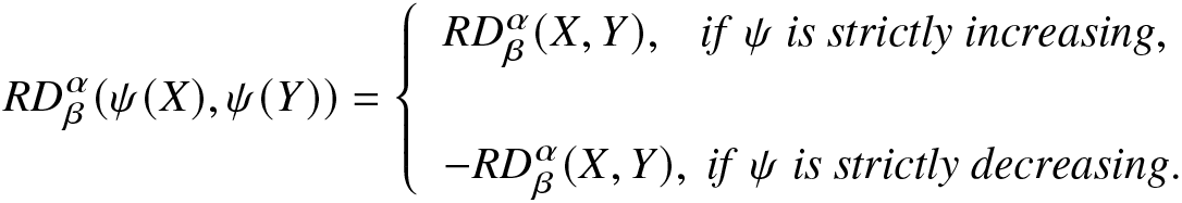 \begin{equation*}
RD^\alpha_\beta(\psi(X),\psi(Y))=\left\{
\begin{array}{ll}
RD^\alpha_\beta(X,Y),~~~
if~\psi~ is ~strictly~ increasing,
\\
\\
-RD^\alpha_\beta(X,Y),~if~ \psi~ is ~strictly~ decreasing.
\end{array}
\right.
\end{equation*}
\begin{equation*}
RD^\alpha_\beta(\psi(X),\psi(Y))=\left\{
\begin{array}{ll}
RD^\alpha_\beta(X,Y),~~~
if~\psi~ is ~strictly~ increasing,
\\
\\
-RD^\alpha_\beta(X,Y),~if~ \psi~ is ~strictly~ decreasing.
\end{array}
\right.
\end{equation*}Proof. The PDFs of  $\psi(X)$ and $\psi(Y)$ are
 \begin{equation*}f_{\psi}(x)=\frac{1}{|\psi^{\prime}(\psi^{-1}(x))|}f(\psi^{-1}(x)) ~~\text{and}~~g_{\psi}(x)=\frac{1}{|\psi^{\prime}(\psi^{-1}(x))|}g(\psi^{-1}(x)),~~ x\in\big(\psi(0),\psi(\infty)\big),\end{equation*}
 respectively. Let us first consider  $\psi(\cdot)$ to be strictly increasing. From (3.1), we have
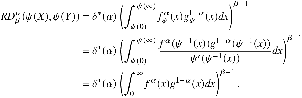 \begin{align*}
RD^\alpha_\beta(\psi(X),\psi(Y))&=\delta^*(\alpha)\left(\int_{\psi(0)}^{\psi(\infty)}f^\alpha_\psi(x)g^{1-\alpha}_\psi(x)dx\right)^{\beta-1}\nonumber\\
&=\delta^*(\alpha)\left(\int_{\psi(0)}^{\psi(\infty)}\frac{f^\alpha(\psi^{-1}(x))g^{1-\alpha}(\psi^{-1}(x))}{\psi^{\prime}(\psi^{-1}(x))}dx\right)^{\beta-1}\nonumber\\
&=\delta^*(\alpha)\left(\int_{0}^{\infty}f^\alpha(x)g^{1-\alpha}(x)dx\right)^{\beta-1}.
\end{align*}
\begin{align*}
RD^\alpha_\beta(\psi(X),\psi(Y))&=\delta^*(\alpha)\left(\int_{\psi(0)}^{\psi(\infty)}f^\alpha_\psi(x)g^{1-\alpha}_\psi(x)dx\right)^{\beta-1}\nonumber\\
&=\delta^*(\alpha)\left(\int_{\psi(0)}^{\psi(\infty)}\frac{f^\alpha(\psi^{-1}(x))g^{1-\alpha}(\psi^{-1}(x))}{\psi^{\prime}(\psi^{-1}(x))}dx\right)^{\beta-1}\nonumber\\
&=\delta^*(\alpha)\left(\int_{0}^{\infty}f^\alpha(x)g^{1-\alpha}(x)dx\right)^{\beta-1}.
\end{align*} Hence,  $RD^\alpha_\beta(\psi(X),\psi(Y))=RD^\alpha_\beta(X,Y)$. We can similarly prove the result for strictly decreasing function $\psi(\cdot)$. This completes the proof of the proposition.
4. Estimation of the RIGF
In this section, we discuss some nonparametric and parametric estimators of the RIGF. A Monte Carlo simulation study is then carried out for the comparison of these two estimators. A real dataset is also analyzed for illustrative purposes.
4.1. Nonparametric estimator of the RIGF
We first propose a nonparametric estimator of the RIGF in (2.5) based on the kernel estimator. Denoted by  $\widehat f(\cdot)$, the kernel estimator of the PDF $f(\cdot)$ is given by
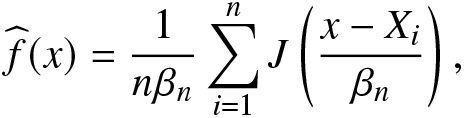 \begin{eqnarray}
\widehat f(x)=\frac{1}{n\beta_n}\sum_{i=1}^{n}J\left(\frac{x-X_i}{\beta_n}\right),
\end{eqnarray}
\begin{eqnarray}
\widehat f(x)=\frac{1}{n\beta_n}\sum_{i=1}^{n}J\left(\frac{x-X_i}{\beta_n}\right),
\end{eqnarray} where  $J(\cdot)~(\ge0)$ is known as kernel and $\{\beta_n\}$ is a sequence of real numbers, known as bandwidths, satisfying $\beta_n\rightarrow0$ and $n\beta_n\rightarrow0$ for $n\rightarrow0.$ For more details, see [Reference Rosenblatt35] and [Reference Parzen32]. Note that the kernel $J(\cdot)$ satisfies the following properties:
(a) It is non-negative, i.e.
$J(x)\ge0;$(b)
$\int J(x)dx=1;$(c) It is symmetric about zero;
(d)
$J(\cdot)$ satisfies the Lipschitz condition.


Thus, based on the kernel estimator, a nonparametric kernel estimator of the RIGF in (2.5) is defined as
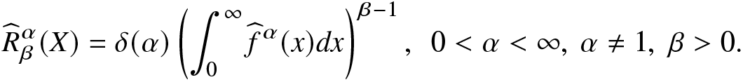 \begin{align}
\widehat {R}^\alpha_\beta(X)=\delta(\alpha)\left(\int_{0}^{\infty}\widehat f^\alpha(x)dx\right)^{\beta-1},~~0 \lt \alpha \lt \infty,~ \alpha\neq1,~ \beta \gt 0.
\end{align}
\begin{align}
\widehat {R}^\alpha_\beta(X)=\delta(\alpha)\left(\int_{0}^{\infty}\widehat f^\alpha(x)dx\right)^{\beta-1},~~0 \lt \alpha \lt \infty,~ \alpha\neq1,~ \beta \gt 0.
\end{align}Further, a nonparametric kernel estimator of the IGF given in (1.3) is obtained as
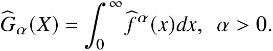 \begin{align}
\widehat {G}_\alpha(X)=\int_{0}^{\infty}\widehat f^\alpha(x)dx,~~\alpha \gt 0.
\end{align}
\begin{align}
\widehat {G}_\alpha(X)=\int_{0}^{\infty}\widehat f^\alpha(x)dx,~~\alpha \gt 0.
\end{align}Next, we carry out a Monte Carlo simulation study to examine the performance of the nonparametric estimators of the RIGF and IGF given in (4.2) and (4.3), respectively. We use Monte Carlo simulation to generate data from Weibull distribution with shape parameter k > 0 and scale parameter λ > 0 for different sample sizes. The SD, AB, and MSE of the kernel-based nonparametric estimators of the RIGF in (4.2) and IGF in (4.3) are then obtained based on 500 replications. Here, we have employed the Gaussian kernel, given by
 \begin{align}
k(z)=\frac{1}{\sqrt{2\pi}}e^{-\frac{z^2}{2}},~-\infty \lt z \lt \infty.
\end{align}
\begin{align}
k(z)=\frac{1}{\sqrt{2\pi}}e^{-\frac{z^2}{2}},~-\infty \lt z \lt \infty.
\end{align} The SD, AB, and MSE of the nonparametric estimators  $\widehat {R}^\alpha_\beta(X)$ and $\widehat {G}_\alpha(X)$ are then computed and are presented for different choices of $n,k,\lambda, \alpha$, and β in Tables 4 and 5. The software “Mathematica” has been used for simulational purposes. From Tables 4 and 5, we observe the following:
• The SD, AB, and MSE decrease as the sample size n increases, verifying the consistency of the proposed estimators;
Table 4. Comparison between the nonparametric estimators of the IGF in (4.3) and RIGF in (4.2) in terms of the AB, MSE, and SD for different choices of α, β,
$k,\lambda$, and n.Table 5. Continuation of Table 8.
• The nonparametric estimator of the RIGF performs better than that of the IGF in terms of the SD, AB, and MSE.


4.2. Parametric estimator of the RIGF
In the previous subsection, we examined the performance of the nonparametric estimators of both RIGF and IGF. Here, we will focus on the parametric estimation of the RIGF and IGF when the probability distribution is Weibull. For the Weibull distribution with shape parameter k > 0 and scale parameter λ > 0, the RIGF and IGF are, respectively, given by
 \begin{align}
R^\alpha_\beta(X)=\delta(\alpha)\left(\int_{0}^{\infty}\Big\{\frac{k}{\lambda}\Big(\frac{x}{\lambda}\Big)^{k-1}e^{-(\frac{x}{\lambda})^k}\Big\}^\alpha dx\right)^{\beta-1},~~0 \lt \alpha \lt \infty,~ \alpha\neq1,~ \beta \gt 0,
\end{align}
\begin{align}
R^\alpha_\beta(X)=\delta(\alpha)\left(\int_{0}^{\infty}\Big\{\frac{k}{\lambda}\Big(\frac{x}{\lambda}\Big)^{k-1}e^{-(\frac{x}{\lambda})^k}\Big\}^\alpha dx\right)^{\beta-1},~~0 \lt \alpha \lt \infty,~ \alpha\neq1,~ \beta \gt 0,
\end{align}and
 \begin{align}
G_\alpha(X)=\int_{0}^{\infty}\Big\{\frac{k}{\lambda}\Big(\frac{x}{\lambda}\Big)^{k-1}e^{-(\frac{x}{\lambda})^k}\Big\}^\alpha dx,~~\alpha \gt 0.
\end{align}
\begin{align}
G_\alpha(X)=\int_{0}^{\infty}\Big\{\frac{k}{\lambda}\Big(\frac{x}{\lambda}\Big)^{k-1}e^{-(\frac{x}{\lambda})^k}\Big\}^\alpha dx,~~\alpha \gt 0.
\end{align}For the estimation of (4.5) and (4.6), the unknown model parameters k and λ are estimated using the maximum likelihood method. The maximum likelihood estimators (MLEs) of RIGF in (4.5) and IGF in (4.6) are then obtained as
 \begin{align}
\widehat R^\alpha_\beta(X)=\delta(\alpha)\left(\int_{0}^{\infty}\Big\{\frac{\widehat k}{\widehat\lambda}\Big(\frac{x}{\widehat\lambda}\Big)^{\widehat k-1}e^{-(\frac{x}{\widehat\lambda})^{\widehat k}}\Big\}^\alpha dx\right)^{\beta-1},~~0 \lt \alpha \lt \infty,~ \alpha\neq1,~ \beta \gt 0,
\end{align}
\begin{align}
\widehat R^\alpha_\beta(X)=\delta(\alpha)\left(\int_{0}^{\infty}\Big\{\frac{\widehat k}{\widehat\lambda}\Big(\frac{x}{\widehat\lambda}\Big)^{\widehat k-1}e^{-(\frac{x}{\widehat\lambda})^{\widehat k}}\Big\}^\alpha dx\right)^{\beta-1},~~0 \lt \alpha \lt \infty,~ \alpha\neq1,~ \beta \gt 0,
\end{align}and
 \begin{align}
\widehat G_\alpha(X)=\int_{0}^{\infty}\Big\{\frac{\widehat k}{\widehat\lambda}\Big(\frac{x}{\widehat\lambda}\Big)^{\widehat k-1}e^{-(\frac{x}{\widehat\lambda})^{\widehat k}}\Big\}^\alpha dx,~~\alpha \gt 0,
\end{align}
\begin{align}
\widehat G_\alpha(X)=\int_{0}^{\infty}\Big\{\frac{\widehat k}{\widehat\lambda}\Big(\frac{x}{\widehat\lambda}\Big)^{\widehat k-1}e^{-(\frac{x}{\widehat\lambda})^{\widehat k}}\Big\}^\alpha dx,~~\alpha \gt 0,
\end{align} where  $\widehat k$ and $\widehat \lambda$ are the MLEs of the unknown model parameters k and λ, respectively. To obtain the SD, AB, and MSE values of $\widehat R^\alpha_\beta(X)$ in (4.7) and $\widehat G_\alpha(X)$ in (4.8), we carry out a Monte Carlo simulation using R software with 500 replications. The SD, AB, and MSE values are then obtained for different choices of parameters α (for fixed β = 1.1, k = 2, and λ = 1.5), β (for fixed α = 0.3, k = 2, and λ = 1), k (for fixed α = 0.3, β = 0.5, and λ = 1), λ (for fixed α = 0.3, β = 0.5, and k = 2), and sample sizes $n=150, 300, 500$. We have presented the SD, AB, and MSE in Tables 6 and 7. We observe the following:
• The values of the SD, AB, and MSE decrease as the sample size n increases for all cases of the parameters
$\alpha, \beta$, k, and λ;Table 6. Comparison between the parametric estimators of the IGF in (4.8) and RIGF in (4.7) in terms of the SD, AB, and MSE for different choices of
$\alpha, \beta, k, \lambda$, and n.Table 7. Continuation of Table 6.
• In general, the SD, AB, and MSE values of the parametric estimator of the RIGF are lesser than those of the IGF, implying a better performance of the estimator of the proposed RIGF than IGF;
• Similar behavior is observed for other choices of the parameters;
• It is observed from Tables 4–7 that the parametric estimator in (4.7) performs better than the nonparametric estimator in (4.2) based on the values of AB and MSE for Weibull distribution, as one would expect.


5. Real data analysis
We consider a real dataset related to the failure times (in minutes) of 15 electronic components in an accelerated life test. The dataset is taken from [Reference Lawless26], which is provided in Table 5. For the purpose of numerical illustration, we use here the Gaussian kernel given in (4.4). Here, we consider four statistical models: exponential (EXP), Weibull, inverse exponential half logistic (IEHL), and log-logistic (LL) distributions to check the best-fitted model for this dataset. The negative log-likelihood criterion  $(-\ln L)$, Akaike-information criterion (AIC), AICc, and Bayesian information criterion (BIC) have all been used as measures of fit. From Table 9, we notice that the exponential distribution fits the dataset better than other considered distributions since the values of all the measures are smaller than those for other distributions, namely, Weibull, IEHL, and LL. The value of the MLE of the unknown model parameter λ is 0.036279. We have used 500 bootstrap samples with size n = 15 and chose
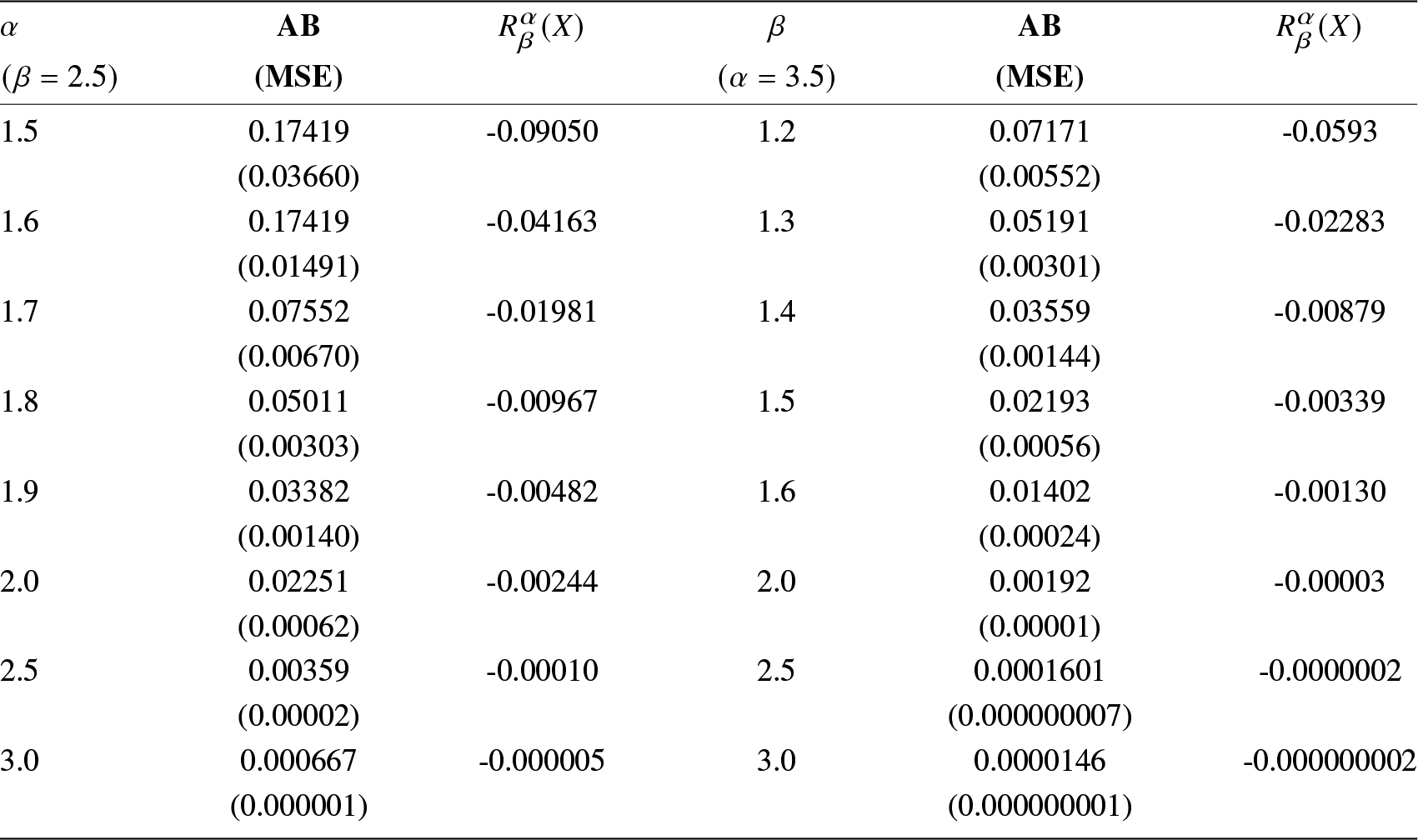
  $\beta_n=0.35$ for computing purposes. The values of AB and MSE for different choices of α (for fixed β = 2.5) and β (for fixed α = 3.5) are presented in Table 10. We observe that the values of AB and MSE all become smaller for larger values of n, verifying the consistency of the proposed estimator.
Table 8. The dataset on failure times (in minutes), of electronic components.

Table 9. The MLEs, BIC, AICc, AIC, and negative log-likelihood values of some statistical models for the real dataset in Table 5.
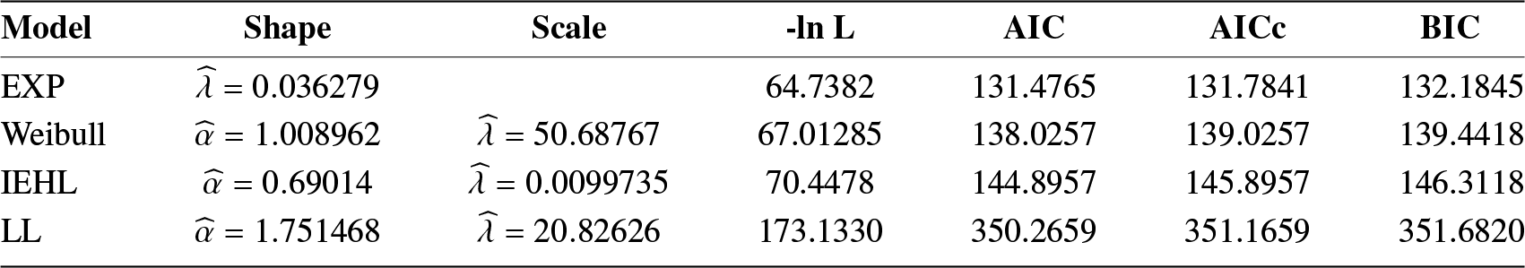
Table 10. The AB, MSE of the nonparametric estimator of the RIGF, and the value of  $R^\alpha_\beta(X)$ based on the real dataset in Table 5 for different choices of α (for fixed β = 2.5) and β (for fixed α = 3.5).
6. Applications
In this section, we discuss some applications of the proposed RIGF. At the end of this section, we highlight that the newly proposed RIGF can be used as an alternative tool to measure uncertainty. First, we discuss its application in reliability engineering.
Application in reliability engineering
Coherent systems are essential in both theoretical and practical contexts because they provide a clear and structured way to analyze, design, and model complex systems. Their predictability, robustness, and applicability across various fields make them indispensable in ensuring the reliability, safety, and efficiency of systems in real-world applications. Here, we propose the RIGF of coherent systems and discuss its properties.
We consider a coherent system with n components and lifetime of the coherent system is denoted by T. For details of a coherent system, one may refer to [Reference Navarro27]. The random lifetimes of n components of the coherent system are identically distributed (i.d.) with a common CDF and PDF  $F(\cdot)$ and $f(\cdot)$, respectively. The CDF and PDF of T are defined as
 \begin{align*}
F_T(x)=q(F(x)) ~~~~~\text{and}~~~~~f_T(x)=q'(F(x))f(x),
\end{align*}
\begin{align*}
F_T(x)=q(F(x)) ~~~~~\text{and}~~~~~f_T(x)=q'(F(x))f(x),
\end{align*} respectively, where  $q:[0,1]\rightarrow[0,1]$ is the distortion function (see [Reference Navarro, del Águila, Sordo and Suárez-Llorens28]) and $q'\equiv\frac{dq}{dx}$. We recall that the distortion function depends on the structure of a system and the copula of the component lifetimes. It is an increasing and continuous function with $q(0)=0$ and $q(1)=1$. Several researchers studied various information measures for coherent systems. In this direction, readers may refer to [Reference Calì, Longobardi and Navarro3, Reference Toomaj, Sunoj and Navarro43], [Reference Saha and Kayal36], and [Reference Saha and Kayal38]. The RIGF of T can be expressed as
 \begin{align}
R_\beta^\alpha(T)
=\delta(\alpha)\bigg(\int_{0}^{\infty}\psi_\alpha\big(F_T(x)\big)dx\bigg)^{\beta-1}
=\delta(\alpha)\bigg(\int_{0}^{1}\frac{\psi_\alpha\big(q(u)\big)}{f(F^{-1}(u))}du\bigg)^{\beta-1},
\end{align}
\begin{align}
R_\beta^\alpha(T)
=\delta(\alpha)\bigg(\int_{0}^{\infty}\psi_\alpha\big(F_T(x)\big)dx\bigg)^{\beta-1}
=\delta(\alpha)\bigg(\int_{0}^{1}\frac{\psi_\alpha\big(q(u)\big)}{f(F^{-1}(u))}du\bigg)^{\beta-1},
\end{align} where  $\psi_\alpha(u)=f^\alpha_T(F^{-1}_T(u))$, for $0\le u\le1$.
Next, we consider an example to obtain the RIGF of a coherent system.
Example 6.1. Suppose  $X_1,X_2,$ and X 3 denote the independent lifetimes of the components of a coherent system. Assume that they all follow power distribution with CDF $F(x)=x^a,~x\in[0,1]$ and a > 0. We take a parallel system with lifetime $T=X_{3:3}=\max\{X_1,X_2,X_3\}$ whose distortion function is $q(u)=u^3,~0\le u\le1$. Thus, from (6.2), the RIGF of the coherent system, for $0 \lt \alpha \lt \infty,~\alpha \neq1$ and β > 0, is obtained as
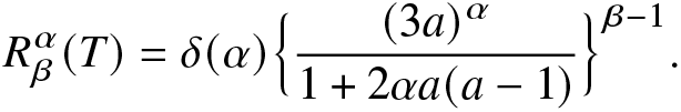 \begin{align*}
R^\alpha_\beta(T)=\delta(\alpha)\Big\{\frac{(3a)^\alpha}{1+2\alpha a(a-1)}\Big\}^{\beta-1}.
\end{align*}
\begin{align*}
R^\alpha_\beta(T)=\delta(\alpha)\Big\{\frac{(3a)^\alpha}{1+2\alpha a(a-1)}\Big\}^{\beta-1}.
\end{align*}In order to check the behavior of the RIGF of a coherent system with respect to β in Example 6.1, its graphs are plotted in Figure 4 for different values of a.
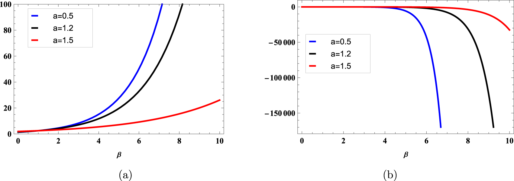
Figure 4. Graphs of the RIGF of parallel system for (a) α = 0.6 and (b) α = 1.5 in Example 6.1. Here, we have considered  $a=0.5,~1.2,~1.5$.
Next, we establish a relationship between the RIGF of a coherent system and that of its components.
Proposition 6.2. Suppose T is the lifetime of a coherent system with identically distributed components and  $q(\cdot)$ is a distortion function. Assume that X is the component lifetime of the coherent system with CDF and PDF $F(\cdot)$ and $f(\cdot)$, respectively, and $\psi_\alpha(u)=f^\alpha_T(F^{-1}_T(u))$, $\phi_\alpha(u)=f^\alpha(F^{-1}(u))$. If $\psi_\alpha(q(u))\ge(\le)\phi_\alpha(u)$ for $0\le u\le 1$, then
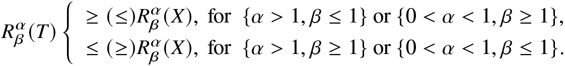 \begin{equation*}
R^\alpha_\beta(T)\left\{
\begin{array}{ll}
\ge (\le) R^\alpha_\beta(X),~
\text{for}~~\{\alpha \gt 1,\beta\le1\}~\text{or}~\{0 \lt \alpha \lt 1,\beta\ge1\},
\\
\le (\ge) R^\alpha_\beta(X),~\text{for}~~\{\alpha \gt 1,\beta\ge1\}~\text{or}~\{0 \lt \alpha \lt 1,\beta\le1\}.
\end{array}
\right.
\end{equation*}
\begin{equation*}
R^\alpha_\beta(T)\left\{
\begin{array}{ll}
\ge (\le) R^\alpha_\beta(X),~
\text{for}~~\{\alpha \gt 1,\beta\le1\}~\text{or}~\{0 \lt \alpha \lt 1,\beta\ge1\},
\\
\le (\ge) R^\alpha_\beta(X),~\text{for}~~\{\alpha \gt 1,\beta\ge1\}~\text{or}~\{0 \lt \alpha \lt 1,\beta\le1\}.
\end{array}
\right.
\end{equation*}Proof. Consider  $0 \lt \alpha \lt 1$, $\beta\ge1$ and $\psi_\alpha(q(u))\ge\phi_\alpha(u)$. Then,
 \begin{align}
\frac{\psi_\alpha(q(u))}{f(F^{-1}(u))}\ge \frac{\phi_\alpha(u)}{f(F^{-1}(u))}
\Rightarrow\delta(\alpha)\bigg(\int_{0}^{1}\frac{\psi_\alpha(q(u))}{f(F^{-1}(u))}du\bigg)^{\beta-1}&\ge\delta(\alpha)\bigg(\int_{0}^{1} \frac{\phi_\alpha(u)}{f(F^{-1}(u))}du\bigg)^{\beta-1},
\end{align}
\begin{align}
\frac{\psi_\alpha(q(u))}{f(F^{-1}(u))}\ge \frac{\phi_\alpha(u)}{f(F^{-1}(u))}
\Rightarrow\delta(\alpha)\bigg(\int_{0}^{1}\frac{\psi_\alpha(q(u))}{f(F^{-1}(u))}du\bigg)^{\beta-1}&\ge\delta(\alpha)\bigg(\int_{0}^{1} \frac{\phi_\alpha(u)}{f(F^{-1}(u))}du\bigg)^{\beta-1},
\end{align} from which the result  $R^\alpha_\beta(T)\ge R^\alpha_\beta(X)$ follows directly. Proofs for other cases are similar and are therefore omitted.
In the following proposition, we establish that two coherent systems are comparable based on the proposed generating function. The dispersive ordering has been used for this purpose.
Proposition 6.3. Let T 1 and T 2 be the lifetimes of two different coherent systems with the same structure and respective identically distributed component lifetimes  $X_1,\cdots,X_n$ and $Y_1,\cdots,Y_n$ with the same copula. The common CDFs and PDFs for $X_1,\cdots,X_n$ and $Y_1,\cdots,Y_n$ are $F_X(\cdot)$, $f_X(\cdot)$ and $F_Y(\cdot)$, $f_Y(\cdot)$, respectively, and $\psi_\alpha(u)=f^\alpha_T(F^{-1}_T(u)),~0\le u\le1$. If $X\le_{disp}Y$, then
(A)
$R^\alpha_\beta(T_1)\le R^\alpha_\beta(T_2),$ for
$\{\alpha \gt 1,\beta\le1\}$ or
$\{0 \lt \alpha \lt 1,\beta\ge1\}$,(B)
$R^\alpha_\beta(T_1)\ge R^\alpha_\beta(T_2),$ for
$\{\alpha \gt 1,\beta\ge1\}$ or
$\{0 \lt \alpha \lt 1,\beta\le1\}$.


Proof. (A) Note that both systems with lifetimes T 1 and T 2 have a common distortion function  $q(\cdot)$, since the systems have the same structure and the same copula. Under the assumption, we have $X\le_{disp}Y$, which implies $f_X(F_X^{-1}(u))\ge f_Y(F_Y^{-1}(u)),~\forall~ 0\le u\le 1$. Thus,
 \begin{align}
\frac{\psi_\alpha(q(u))}{f_X(F^{-1}_X(u))}\le \frac{\psi_\alpha(q(u))}{f_Y(F^{-1}_Y(u))}.
\end{align}
\begin{align}
\frac{\psi_\alpha(q(u))}{f_X(F^{-1}_X(u))}\le \frac{\psi_\alpha(q(u))}{f_Y(F^{-1}_Y(u))}.
\end{align}Hence, the result follows directly from (6.4). Hence the required result.
(B) The proof is quite similar to that of Part (A) and is therefore not presented here.
Next, we obtain bounds of the RIGF  $R^\alpha_\beta(T)$ in terms of $R^\alpha_\beta(X)$ when a coherent system has identically distributed components.
Proposition 6.4. Suppose that T and X are, respectively, the lifetimes of a coherent system and the component of this coherent system. Further, assume that the coherent system has identically distributed components with CDF  $F(\cdot)$ and PDF $f(\cdot)$, and its distortion function is $q(\cdot)$. Take $\psi_\alpha(u)=f^\alpha_T(F^{-1}_T(u))$ and $\phi_\alpha(u)=f^\alpha(F^{-1}(u)),$ for $0\le u\le1$. Then, we have
(A)
$\xi_{1,\alpha}R^\alpha_\beta(X)\le R^\alpha_\beta(T)\le \xi_{2,\alpha}R^\alpha_\beta(X)$, for
$\{\alpha \gt 1,\beta\le1\}$ or
$\{0 \lt \alpha \lt 1,\beta\ge1\}$,(B)
$\xi_{1,\alpha}R^\alpha_\beta(X)\ge R^\alpha_\beta(T)\ge \xi_{2,\alpha}R^\alpha_\beta(X)$, for
$\{\alpha \gt 1,\beta\ge1\}$ or
$\{0 \lt \alpha \lt 1,\beta\le1\}$.


where  $\xi_{1,\alpha}=\big(\inf_{u\in(0,1)}\frac{\psi_\alpha(q(u))}{\phi_\alpha(u)}\big)^{\beta-1}$ and $\xi_{2,\alpha}=\big(\sup_{u\in(0,1)}\frac{\psi_\alpha(q(u))}{\phi_\alpha(u)}\big)^{\beta-1}$.
Proof. (A) From (6.2), we obtain
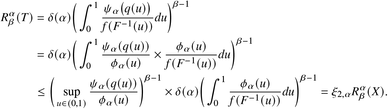 \begin{align*}
R^\alpha_\beta(T)&=\delta(\alpha)\bigg(\int_{0}^{1}\frac{\psi_\alpha\big(q(u)\big)}{f(F^{-1}(u))}du\bigg)^{\beta-1}\\
&=\delta(\alpha)\bigg(\int_{0}^{1}\frac{\psi_\alpha(q(u))}{\phi_\alpha(u)}\times\frac{\phi_\alpha(u)}{f(F^{-1}(u))}du\bigg)^{\beta-1}\\
&\le\bigg(\sup_{u\in(0,1)}\frac{\psi_\alpha(q(u))}{\phi_\alpha(u)}\bigg)^{\beta-1}\times\delta(\alpha)\bigg(\int_{0}^{1}\frac{\phi_\alpha(u)}{f(F^{-1}(u))}du\bigg)^{\beta-1}=\xi_{2,\alpha}R^\alpha_\beta(X).
\end{align*}
\begin{align*}
R^\alpha_\beta(T)&=\delta(\alpha)\bigg(\int_{0}^{1}\frac{\psi_\alpha\big(q(u)\big)}{f(F^{-1}(u))}du\bigg)^{\beta-1}\\
&=\delta(\alpha)\bigg(\int_{0}^{1}\frac{\psi_\alpha(q(u))}{\phi_\alpha(u)}\times\frac{\phi_\alpha(u)}{f(F^{-1}(u))}du\bigg)^{\beta-1}\\
&\le\bigg(\sup_{u\in(0,1)}\frac{\psi_\alpha(q(u))}{\phi_\alpha(u)}\bigg)^{\beta-1}\times\delta(\alpha)\bigg(\int_{0}^{1}\frac{\phi_\alpha(u)}{f(F^{-1}(u))}du\bigg)^{\beta-1}=\xi_{2,\alpha}R^\alpha_\beta(X).
\end{align*}Hence, the proof of the right-side inequality is completed. The proof of the left-side inequality is similar and is therefore omitted.
(B) The proof is quite similar to that of Part (A) and is therefore omitted.
The following proposition shows that the preceding result can be extended to compare two systems based on the RIGF.
Proposition 6.5. Let T 1 and T 2 be the lifetimes of two coherent systems with identically distributed components with distortion functions q 1 and q 2, respectively. Assume that  $\psi_\alpha(u)=f^\alpha_T(F^{-1}_T(u)),$ for $0\le u\le 1$. Then,
(A)
$\gamma_{1,\alpha}R^\alpha_\beta(T_1)\le R^\alpha_\beta(T_2)\le \gamma_{2,\alpha}R^\alpha_\beta(T_1)$, for
$\{\alpha \gt 1,\beta\le1\}$ or
$\{0 \lt \alpha \lt 1,\beta\ge1\}$,(B)
$\gamma_{1,\alpha}R^\alpha_\beta(T_1)\ge R^\alpha_\beta(T_2)\ge \gamma_{2,\alpha}R^\alpha_\beta(T_1)$, for
$\{\alpha \gt 1,\beta\ge1\}$ or
$\{0 \lt \alpha \lt 1,\beta\le1\}$,


where  $\gamma_{1,\alpha}=\big(\inf_{u\in(0,1)}\frac{\psi_\alpha(q_2(u))}{\psi_\alpha(q_1(u))}\big)^{\beta-1}$ and $\gamma_{2,\alpha}=\big(\sup_{u\in(0,1)}\frac{\psi_\alpha(q_2(u))}{\psi_\alpha(q_1(u))}\big)^{\beta-1}$.
Proof. The proof is similar to that of Proposition 6.4 and is therefore omitted for brevity.
The following result provides additional bounds of the RIGF of the lifetime of a coherent system when the PDF is bounded. The proof is simple, and thus it is omitted.
Proposition 6.6. Consider a coherent system as in Proposition 6.4. Let the CDF and PDF of the components be  $F(\cdot)$ and $f(\cdot)$,respectively, and $\psi_\alpha(u)=f^\alpha_T(F^{-1}_T(u))$, for $0\le u\le1,~0 \lt \alpha \lt \infty,~\alpha\neq1$ and β > 0.
(A) If
$f(x)\le M,~ \forall x\in S$, then
$R^\alpha_\beta(T)\ge(\le)\frac{1}{M^{\beta-1}}\big(\int_{0}^{1}\psi_\alpha(q(u))du\big)^{\beta-1}$, for
$\alpha \lt ( \gt )1$;(B) If
$f(x)\ge L \gt 0,~ \forall x\in S$, then
$R^\alpha_\beta(T)\le (\ge)\frac{1}{L^{\beta-1}}\big(\int_{0}^{1}\psi_\alpha(q(u))du\big)^{\beta-1},$ for
$\alpha \lt ( \gt )1$.


Next, a comparative study is carried out between the proposed RIGF and IGF (according to [Reference Golomb11]), Rényi entropy (according to [Reference Rényi33]), and varentropy (according to [Reference Fradelizi, Madiman and Wang10]) for three different coherent systems with three components. Suppose T and X denote the system’s lifetime and component’s lifetime with PDFs  $f_T(\cdot)$ and $f(\cdot)$ and CDFs $F_T(\cdot)$ and $F(\cdot)$, respectively. The IGF and Rényi entropy of T are
 \begin{align}
I(T)=\int_{0}^{\infty}f^\alpha_T(x)dx
=\int_{0}^{1}\frac{\psi_\alpha\big(q(u)\big)}{f(F^{-1}(u))} du,~~\alpha \gt 0,
\end{align}
\begin{align}
I(T)=\int_{0}^{\infty}f^\alpha_T(x)dx
=\int_{0}^{1}\frac{\psi_\alpha\big(q(u)\big)}{f(F^{-1}(u))} du,~~\alpha \gt 0,
\end{align}and
 \begin{align}
H_{\alpha}(T)=\delta(\alpha)\log\int_{0}^{\infty}f_T^{\alpha}(x)dx
=\delta(\alpha)\log\int_{0}^{1}\frac{\psi_\alpha\big(q(u)\big)}{f(F^{-1}(u))}du,~~\alpha \gt 0~(\ne1),
\end{align}
\begin{align}
H_{\alpha}(T)=\delta(\alpha)\log\int_{0}^{\infty}f_T^{\alpha}(x)dx
=\delta(\alpha)\log\int_{0}^{1}\frac{\psi_\alpha\big(q(u)\big)}{f(F^{-1}(u))}du,~~\alpha \gt 0~(\ne1),
\end{align} where  $\psi_\alpha(q(u))=f^\alpha_T(F^{-1}_T(q(u)))$, respectively. Further, the varentropy of T is
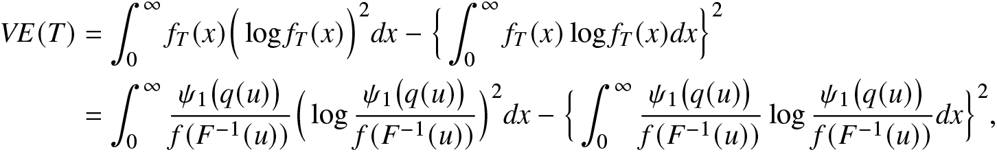 \begin{align}
VE(T)&=\int_{0}^{\infty}f_T(x)\Big(\log f_T(x)\Big)^2dx-\Big\{\int_{0}^{\infty}f_T(x)\log f_T(x)dx\Big\}^2\nonumber\\
&=\int_{0}^{\infty}\frac{\psi_1\big(q(u)\big)}{f(F^{-1}(u))}\Big(\log \frac{\psi_1\big(q(u)\big)}{f(F^{-1}(u))}\Big)^2dx-\Big\{\int_{0}^{\infty}\frac{\psi_1\big(q(u)\big)}{f(F^{-1}(u))}\log \frac{\psi_1\big(q(u)\big)}{f(F^{-1}(u))}dx\Big\}^2,
\end{align}
\begin{align}
VE(T)&=\int_{0}^{\infty}f_T(x)\Big(\log f_T(x)\Big)^2dx-\Big\{\int_{0}^{\infty}f_T(x)\log f_T(x)dx\Big\}^2\nonumber\\
&=\int_{0}^{\infty}\frac{\psi_1\big(q(u)\big)}{f(F^{-1}(u))}\Big(\log \frac{\psi_1\big(q(u)\big)}{f(F^{-1}(u))}\Big)^2dx-\Big\{\int_{0}^{\infty}\frac{\psi_1\big(q(u)\big)}{f(F^{-1}(u))}\log \frac{\psi_1\big(q(u)\big)}{f(F^{-1}(u))}dx\Big\}^2,
\end{align} where  $\psi_1(q(u))=f_T(F^{-1}_T(q(u))).$ Here, we consider the power distribution with CDF $F(x)=\sqrt{x},~x \gt 0$, as a baseline distribution (component lifetime) for illustrative purposes. We take three coherent systems: series system ( $X_{1:3}$), 2-out-of-3 system ( $X_{2:3}$), and parallel system ( $X_{3:3}$) for evaluating the values of $R^\alpha_\beta(T)$ in (6.2), I(T) in (6.5), $H_{\alpha}(T)$ in (6.6), and VE(T) in (6.7). The numerical values of the RIGF, IGF, Rényi entropy, and varentropy for the series, 2-out-of-3, and parallel systems with α = 1.2 and β = 0.5 are reported in Table 11. As expected, from Table 11, we observe that the uncertainty values of the series system are maximum; and minimum for parallel systems considering all information measures, validating the proposed IGF.
Table 11. The values of the RIGF, IGF, Rényi entropy, and varentropy for the series, 2-out-of-3, and parallel systems.
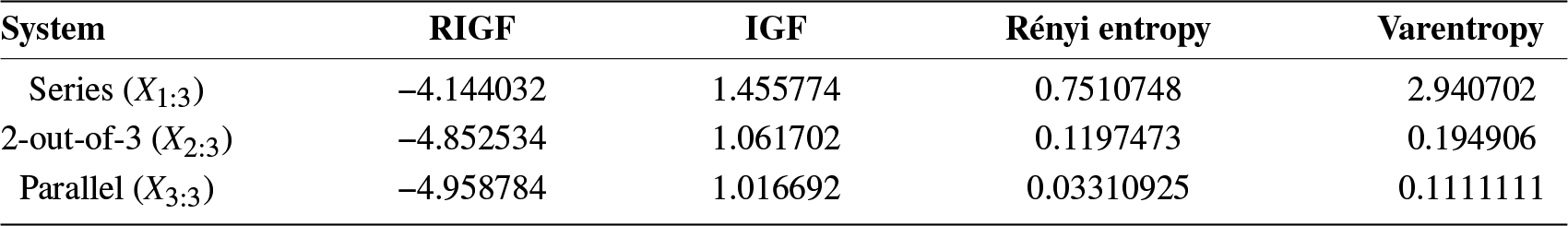
RDIGF and RIGF as model selection criteria
Here, we show that the proposed IGFs, RDIGF and RIGF, can be used as model selection criteria. First, we focus on RDIGF. In this regard, we consider the real dataset, dealing with the failure times (in minutes) of electronic components in an accelerated life test, given in Table 5. We conduct a goodness-of-fit test here. The four statistical models: EXP, Weibull, IEHL, and LL distributions are considered for the test. The values of the test statistics: -ln L, AIC, AICc, BIC, and MLEs of the unknown model parameters are computed and are given in Table 9. From Table 9, we notice that the exponential distribution fits better than other distributions. The sequence of fitness of the statistical models is EXP, Weibull, IEHL, and LL distributions according to the values of −ln L, AIC, AICc, and BIC. Now, we obtain the values of RDIGF between EXP and Weibull (denoted as RDIGF(E, W)), EXP and IEHL (denoted as RDIGF(E, I)), and EXP and LL (denoted as RDIGF(E, L)). The values of RDIGF are given for different choices of α and β in Table 12. The sequence of the values of RDIGF observed is
 \begin{equation*}\mbox{RDIGF}(E,W) \lt \mbox{RDIGF}(E,I) \lt \mbox{RDIGF}(E,L),\end{equation*}
Table 12. The values of RDIGF(E, W), RDIGF(E, I), and RDIGF(E, L), for different choices of α and β.
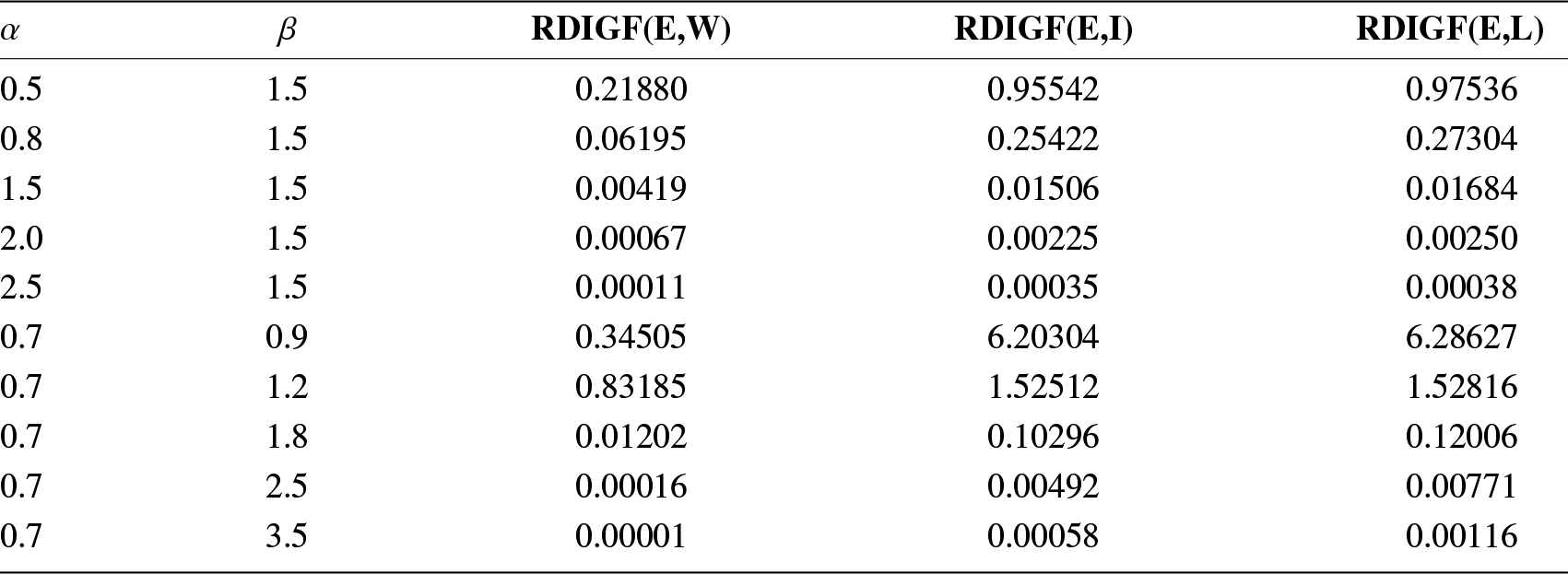
for different choices of α and β, as expected.
Next, we conduct a Monte Carlo simulation study to demonstrate the importance of the RIGF for the purpose of model selection. First, using R software, we generate 500 exponentially distributed random variates with λ = 0.5. Then, we compute the RIGF of this dataset under the assumption that the same set of data comes from
• exponential distribution;
• Weibull distribution;
• Pareto distribution.
For this purpose, the maximum likelihood estimates have been used to calculate the estimated value of RIGF. This process is repeated 1000 times, and then the favorable proportions in each case have been counted. The results so obtained are presented in Table 13, from which we observe that proportion of the RIGF for the exponential model is larger than other proportional values, as expected. From the tabulated values, we also observe that the Weibull distribution will be the better fitting choice than the Pareto distribution.
Table 13. The proportion of the values of the RIGF for exponential, Weibull, and Pareto distributions.
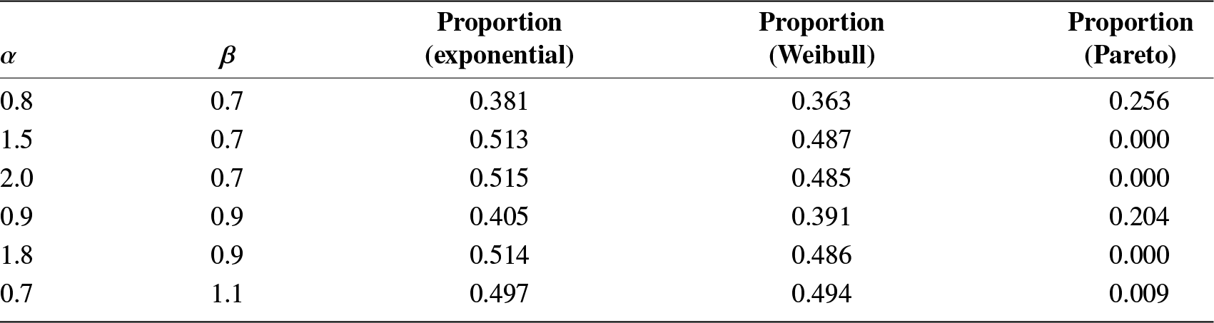
Validation using three chaotic maps
Chaotic maps are mathematical functions that exhibit chaotic behavior, meaning that they are highly sensitive to initial conditions and can generate complex, seemingly random patterns over time, even though they are deterministic in nature. There are various chaotic maps such as logistic maps, Chebyshev maps, and Hénnon maps. These maps are used to model complex, real-world systems that exhibit chaotic behavior, such as weather systems, financial markets, population dynamics in ecology, and even certain physiological processes in biology. In signal processing, chaotic maps can be used for tasks such as compression, encryption, and secure communication. The unpredictability of chaotic signals can help in masking information and making it harder to intercept or decode. These maps are also used in image processing, machine learning, and control theory. Here, we have studied the chaotic behavior of the proposed RIGF for Chebyshev, Hénnon, and logistic maps. Very recently, Kharazmi and Contreras-Reyes [Reference Kharazmi and Contreras-Reyes22] have studied fractional cumulative residual inaccuracy measures in terms of the Chebyshev and logistic maps.
Chebyshev map
The Chebyshev map is defined as
 \begin{align}
x_{r+1}=\cos({s^2 \arccos(x_r)}),~~~~r=1,2,\cdots, n-1,
\end{align}
\begin{align}
x_{r+1}=\cos({s^2 \arccos(x_r)}),~~~~r=1,2,\cdots, n-1,
\end{align} where  $x_r\in[-1,1]$ and s > 0. We have considered the initial value $x_1=0.1$ and sample size n = 10000. For $0 \lt s\le1$, we get $x_r\in[0,1]$ and $x_r\in[-1,1]$ for s > 1.
The bifurcation diagram of the Chebyshev map in (6.8) is presented in Figure 5(a). Using the dataset with size n = 10000, we have estimated the proposed measure RIGF in (4.2). Based on the data extracted from the Chebyshev map, two graphs of the RIGF with respect to β are provided in Figure 5(b) for s = 0.8 and 2.0 when α = 0.01. From Figure 5(a), we notice that the chaos for s > 1 is greater than that for s < 1. From Figure 5(b), we observe that the uncertainty computing via the proposed RIGF for s = 2 (red line) is greater than that when s = 0.8 (black line) for all β, as we would expect; also, they are equal when β = 1.
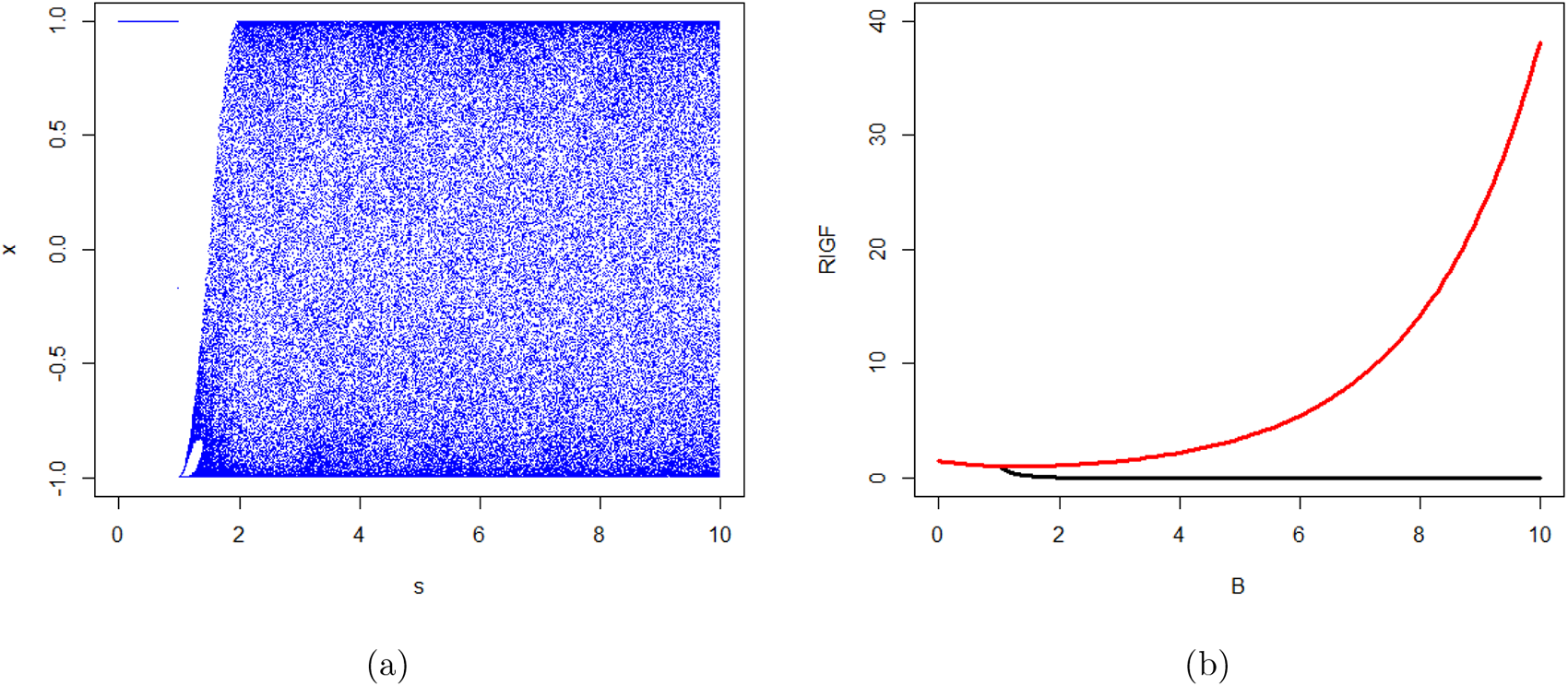
Figure 5. (a) The bifurcation diagram of the Chebyshev map in (6.8) and (b) the plots of the RIGF for the Chebyshev map when s = 0.8 (black) and s = 2.0 (red) with respect to beta (B).
Hénon map
The Hénon map is a discrete-time dynamical system that exhibits chaotic behavior. Note that Michel Hénon first introduced the map as a simplified version of the Poincaré section of the Lorenz model. The Hénon map is defined as
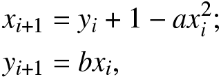 \begin{align}
x_{i+1}&=y_i+1-ax^2_i;\nonumber\\
y_{i+1}&=bx_i,
\end{align}
\begin{align}
x_{i+1}&=y_i+1-ax^2_i;\nonumber\\
y_{i+1}&=bx_i,
\end{align} where  $i=1,2,\ldots,n-1$, and $a,~b \gt 0$. For details, one may refer to [Reference Henon14]. Two factors that determine the map’s dependability are a and b, which for the conventional Hénon map have values of a = 1.4 and b = 0.3. The Hénon map is chaotic for the classical values. For the other values, the Hénon map may be chaotic, intermittent, or converge to a periodic orbit.
Here, we take the initial values  $x_1=0.1$ and $y_1=0.1$, sample size $n=10,000$ with b = 0.3 and α = 0.8. The bifurcation diagram of the Hénnon map is presented in Figure 6(a). The plots of the RIGF in (4.2) based on the Hénon map have been drawn for a = 1.0 (black line), a = 1.2 (blue line), and a = 1.4 (red line) with fixed parameter value b = 0.3 in Figure 6(b). From Figure 6(a), we observe that the chaos is maximum for a = 1.4. From Figure 6(b), as expected, we get the plots of the RIGF, matching with the bifurcation diagram in Figure 6(a). We also notice that the chaos for $\beta\in[0,1)$ is larger than that for β > 1.
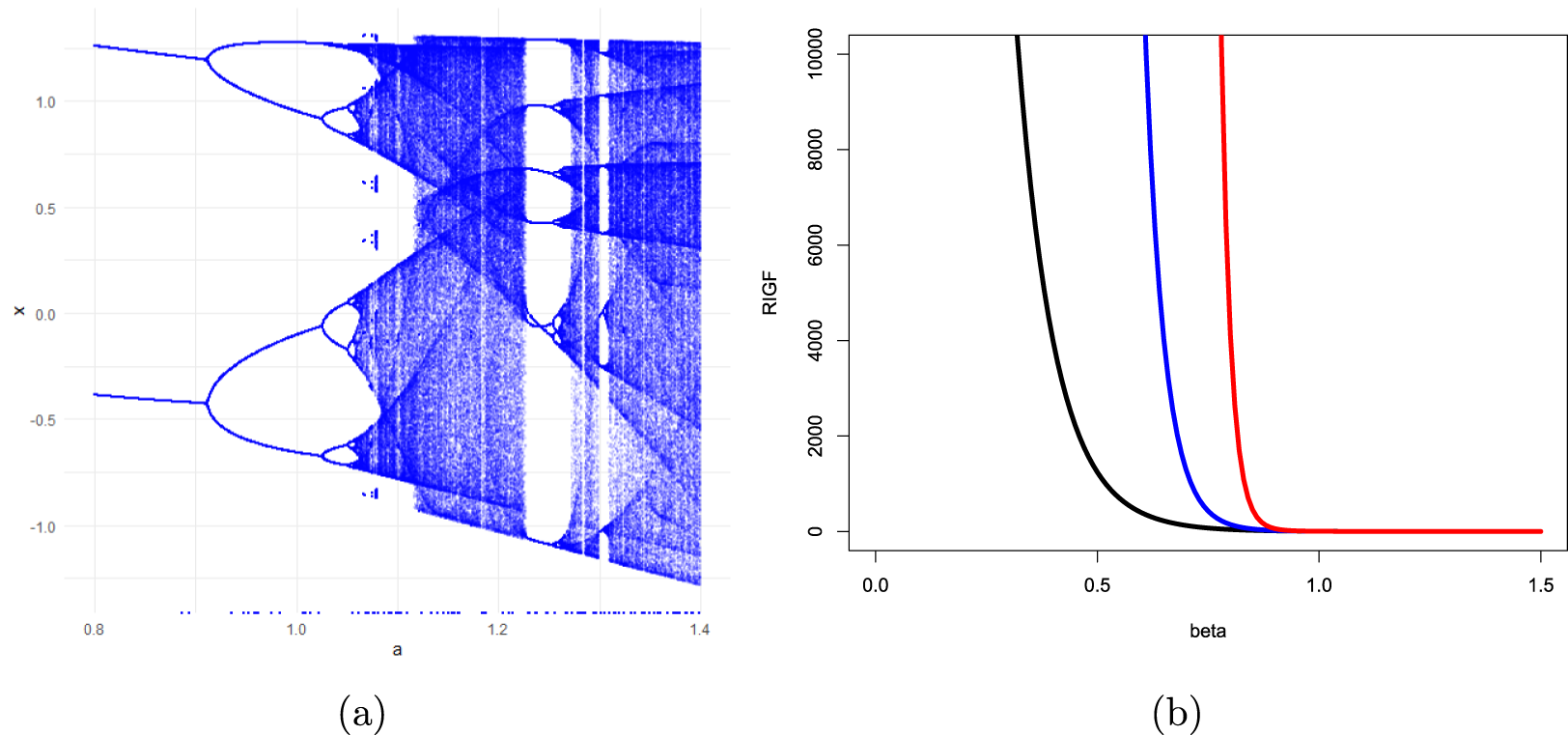
Figure 6. (a) Bifurcation diagram of the Hénon map in (6.9) and (b) the plots of the RIGF of Hénon map for a = 1.4 (red line), a = 1.2 (blue line), and a = 1.0 (black line).
Logistic map
The logistic map used to study the chaotic behavior of a system is defined by
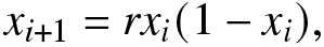 \begin{align}
x_{i+1}=rx_i(1-x_i),
\end{align}
\begin{align}
x_{i+1}=rx_i(1-x_i),
\end{align} where  $i=1,2,\ldots,n-1$, and $0\le r\le4$. For details about this map, see [Reference Feigenbaum8]. Here, we consider the initial value $x_1=0.1$ and sample size $n=10,000$ for the study of the chaotic behavior of the proposed measure RIGF in (4.2). The bifurcation diagram of the logistic map in (6.10) is shown in Figure 7(a). The plots of the RIGF of the logistic map with respect to β for r = 3.4 (black line), 3.8 (blue line), and 4.0 (red line) are presented in Figure 7(b) for α = 0.01. From 7(b), we observe that the uncertainty for r = 4 is greater than that for r = 3.4 and 3.8 when β > 1 and they are equal for β = 1, as expected. We also observe that the RIGF of logistic map decreases when β increases.
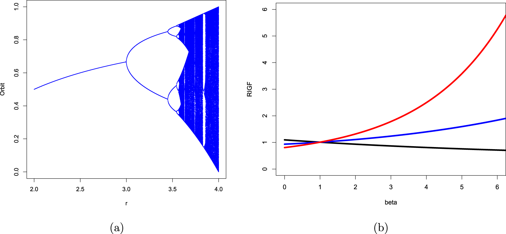
Figure 7. (a) Bifurcation diagram of the logistic map in (6.10) and (b) the plots of the RIGF of logistic map for r = 4 (red line), r = 3.8 (blue line), and r = 3.4 (black line).
7. Concluding comments
In this paper, we have proposed some new IGFs, which produce some well-known information measures, such as Rényi entropy, Rényi divergence, and Jensen-Rényi divergence measures. We have illustrated the generating functions with various examples. We have shown that the RIGF is shift-independent. Various bounds have been obtained as well. Further, the RIGF has been expressed in terms of the Shannon entropy of order q > 0. We have obtained the RIGF for the escort distribution. It has been observed that the RDIGF reduces to the RIGF when the random variable Y is uniformly distributed in the interval  $(0,1)$. The RDIGF has been studied for generalized escort distribution. Further, the effect of this IGF on monotone transformations has been discussed. A kernel-based nonparametric estimator and a parametric estimator of the RIGF have been proposed. A Monte Carlo simulation study has been conducted for both nonparametric and parametric estimators. The performance of the nonparametric as well as parametric estimators of the proposed RIGF and IGF has been studied based on the SD, AB, and MSE. Superior performance has been observed for the newly proposed estimator of RIGF. In addition, it has been shown that the parametric estimator performs better than the nonparametric estimator of the RIGF for the case of Weibull distribution, as one would expect. Further, a real dataset on the failure times (in minutes) of 15 electronic components has been used for illustrative purposes. Few possible applications of the proposed RIGF and RDIGF have been explored. For three coherent systems, we have computed the values of the proposed RIGF, IGF, Renyi entropy, and varentropy. It has been observed that the RIGF has similar behavior with other well-known measures. Further, a study regarding the usefulness of the RDIGF and RIGF as model selection criteria has been conducted. Finally, three chaotic maps have been considered and analyzed to validate the use of the IGFs introduced here.
Acknowledgements
The authors would like to thank the Editor, Editorial Board Member: Prof. Min Xie, and Referees for all their helpful comments and suggestions, which led to the substantial improvements. Shital Saha thanks the University Grants Commission (Award No. 191620139416), India, for financial assistantship to carry out this research work. The first two authors thank the research facilities provided by the Department of Mathematics, National Institute of Technology Rourkela, India.


 Open access